Introduction - LMU

Munich Personal RePEc Archive

Understanding international crime

trends: The legacy of preschool lead

exposure

Nevin, Rick

15 February 2007

Online at https://mpra.ub.uni-muenchen.de/35338/

MPRA Paper No. 35338, posted 11 Dec 2011 02:16 UTC

Understanding International Crime Trends: The Legacy of Preschool Lead Exposure – Page 1

Understanding International Crime Trends:

The Legacy of Preschool Lead Exposure

February 15, 2007

Rick Nevin

National Center for Healthy Housing

Notice: This is an author’s version of a work that was accepted for publication by Environmental Research. Changes

that resulted from the publishing process, such as peer review, editing, corrections, structural formatting, and other

quality control mechanisms may not be reflected in this document. Changes may have been made to this work since

it was submitted for publication. A definitive version was subsequently published in Environmental Research,

Volume 104, Issue 3, July 2007, Pages 315-336.

http://dx.doi.org/10.1016/j.envres.2007.02.008

http://dx.doi.org/10.1016/j.envres.2007.02.008


Understanding International Crime Trends: The Legacy of Preschool Lead Exposure

Abstract

This study shows a very strong association between preschool blood lead and subsequent crime

rate trends over several decades in the USA, Britain, Canada, France, Australia, Finland, Italy,

West Germany, and New Zealand. The relationship is characterized by best-fit lags (highest R2

and t-value for blood lead) consistent with neurobehavioral damage in the first year of life and the

peak age of offending for index crime, burglary, and violent crime. The impact of blood lead is

also evident in age-specific arrest and incarceration trends. Regression analysis of average 1985-

1994 murder rates across USA cities suggests that murder could be especially associated with

more severe cases of childhood lead poisoning.

Key Words: Lead Poisoning, Crime, IQ, Behavior, Violence


1. Introduction

Crime trends can be related to demographic, cultural, economic, and law enforcement trends, but

the sharp 1990s USA crime decline was not anticipated by such theories. Fox (1996) forecasted a

1995-2005 increase in teen murderers due to a rising population of teens, and especially black

teens. Those demographic trends were overwhelmed by a 77% fall in the juvenile murder arrest

rate from 1993-2003, led by an 83% decline for black youths. (Office of Juvenile Justice and

Delinquency Prevention, 2004) DiIulio (1996) warned juvenile crime was “getting worse” due to

children growing up around “criminal adults” in “fatherless … jobless settings”. Juvenile arrests

then plummeted as adult arrest rates changed little, with the percent of children raised by single

parents at record highs, and fell further as unemployment rose after 2000. Levitt (2004) reviews

evidence that unemployment has a “statistically significant but substantively small relationship”

with property crime and no effect on violence, but says the 1990s crime decline can be explained

by rising police per capita and incarceration rates and the early-1970s abortion of “unwanted”

children, presumed more likely to offend. (Donohue & Levitt, 2001) Levitt admits this model

cannot explain 1973-1991 trends, when crime and incarceration rates surged as police per capita

changed little. (Harrison, 2000; Reaves, 2003; Bureau of Justice Statistics, 2006) International

crime trends are even more vexing. (Ferrington et al., 2004) Britain legalized abortion before the

USA, but violent crime rose in Britain and across Europe and Oceana in the 1990s despite rising

incarceration rates, rising or unchanged police per capita, and declines in the age 15-19 share of

the population (Barclay & Tavares, 2003; U.S. Census, 2004)

Criminal offending is also associated with brain damage (Raine et al., 1998), and the use of lead

in paint and gasoline caused global neurotoxin exposure. Elevated maternal and preschool blood

lead can impair formative brain growth, as “incomplete development of the blood-brain barrier in


fetuses and in very young children (up to 36 months of age) increases the risk of lead’s entry into

the developing nervous system, which can result in prolonged or permanent neurobehavioral

disorders.” (Agency for Toxic Substances and Disease Registry, 2000) Preschool blood lead over

70 ug/dL (micrograms of lead per deciliter of blood) can cause seizures and death, blood lead

over 10 ug/dL is harmful to learning and behavior and there is no lower blood lead threshold for

IQ losses. (U.S. Centers for Disease Control and Prevention, 1991; Schwartz, 1994; Canfield et.

al., 2003) The half-life of lead in blood is 30 days, but preschool blood lead often changes slowly

due to continuing exposure, and that lead burden accumulates in teeth and bones. (World Health

Organization, 1995) Needleman (2003) found youths with high bone lead are twice as likely to

be delinquent, after controlling for confounders. Other studies also link preschool lead exposure

to aggressive and delinquent adolescent behavior and later criminal violence. (Denno, 1990;

Needleman et al., 1996; Dietrich et al., 2001)

Stretesky and Lynch (2001) found USA counties with high 1990 air lead, mostly from industrial

emissions, had 1989-1991 murder rates four times higher than counties with low air lead, after

controlling for nine air pollutants and six sociological factors. This study likely reflects 1970s

additive preschool lead exposure, because if murder were much affected by contemporaneous air

lead then the homicide rate would have fallen as gasoline lead and air lead fell over 70% from

1975-1984. (U.S. Environmental Protection Agency, 1986) Most 1990 lead-emitting facilities

were in operation for decades, in areas with older housing and some traffic, so 1989-1991 murder

rates likely reflected higher 1970s blood lead where children had additive exposure to lead in

paint and gasoline and industrial emissions. Nevin (2000) found 1941-1975 gasoline lead use

explained 90% of the 1964-1998 variation in USA violent crime. The best statistical-fit lag of 23-

years is consistent with neural damage in infancy and peak ages of violent offending. Nevin


showed a best-fit lag of 18 years for gasoline lead versus 1960-1998 murders, and 21 years for per

capita paint lead use versus 1900-1959 murders. The difference in best-fit murder lags is

consistent with when paint and gas lead most affected preschool lead exposure. Gas lead settled

over a few weeks or months, and heavily-leaded circa-1900 lead paint deteriorated via “chalking”

after three years. (Schwartz & Pitcher, 1989; van Alphen, 1998)

1.1 Lead Exposure Pathways and Population Blood Lead Trends

Elevated blood lead can be due to lead paint chip ingestion, inhaled air lead, and other pathways,

but paint and gasoline had especially pervasive effects due to lead contaminated dust ingested via

normal hand-to-mouth activity as children crawl. Average daily lead ingested by two-year-olds

exposed to dust contaminated by interior lead paint is similar to the average for two-year-olds

exposed to dust contaminated by settled city air lead, and average two-year-old lead ingestion via

dust is many times average ingestion via inhaled air lead, dietary lead (from air lead settled on

crops and/or lead solder in food and beverage cans), or other pathways. (U.S. Environmental

Protection Agency, 1986)

Lead used in paint accounted for almost a third of total USA lead output from 1900-1914, when

the USA produced over 40% of world lead output. (Nevin, 2000; U.S. Geological Survey, 2006)

The high USA per capita use of lead in early-1900s paint caused more severe USA lead paint

hazards throughout the 20th

Century. The lead share of USA paint pigments fell from near 100%

in 1900 to 35% in the mid-1930s (Meyer & Mitchell, 1943), but the USA did not ban residential

lead paint until 1978. Pre-1940 and 1940-1959 homes each accounted for about a third of USA

homes in the early-1980s, and about 80% of pre-1940 and 46% of 1940-1959 homes still had

some interior lead paint in 1999. (U.S. Census, 1977-2003; Jacobs et al, 2002) Since the 1980s


USA phase out of lead in gasoline, preschool blood lead prevalence over 10 ug/dL has tracked

USA trends in the prevalence of housing with dust hazards caused by interior lead paint. (Jacobs

& Nevin, 2006) Trends in preschool blood lead prevalence over 10 ug/dL are especially affected

by widespread exposure to lead dust hazards, but paint chip ingestion is often a factor in severe

lead poisoning. A 1989-1990 study found that children with x-ray evidence of recent paint chip

ingestion had average blood lead of 63 ug/dL. (McElvaine et al. 1992)

Per capita use of lead in gasoline surged in the USA after World War II, and rose at a slower rate

in nations with lower per capita gasoline consumption. Lead emissions from urban traffic caused

greater lead exposure for city children because 10% of lead emissions settled within 100 meters of

the road and 55% within 20 kilometers, however atmospheric emissions also affected blood lead

in areas with little traffic. (Organization for Economic Cooperation and Development, 1993)

National trends in average blood lead and the use of lead in gasoline were highly correlated, with

median R2 of 0.94 in Greece, Spain, South Africa, Venezuela, Belgium, Sweden, Mexico,

Finland, Canada, New Zealand, Italy, Switzerland, Britain and the USA. (Thomas et al., 1999)

Children exposed to lead in paint and gasoline had a greater risk of elevated blood lead because

lead ingestion is additive, but average blood lead closely tracked gasoline lead use due to slow

changes in lead paint exposure after the 1930s. Lead exposure also spanned a wide range due to

gas lead fallout related to city size and road proximity. USA cities with population over a million

had early-1960s ambient air lead twice that in cities of 250,000 to a million, which had air lead

40% higher than cities of 100,000-250,000. Air lead beside a heavily trafficked Cincinnati street

(2150 cars/hour or about 50,000 cars/day) was 15 times the city’s ambient air lead. (U.S. Public

Health Service, 1966; 1965) Severe lead exposure was an unrecognized consequence of locating

public housing beside highways. For example, Chicago’s long narrow Robert Taylor Homes


project that opened in 1962 was all within about 400 meters of 1963 Dan Ryan expressway traffic

of 150,000 vehicles per day. (American Highway Users Alliance, 2004)

Many children had additive 1950-1970 exposure to city air lead and severely deteriorated lead

paint in circa-1900 slum housing. “In the 1960s many inner city hospitals had large numbers of

comatose and convulsing children with lead poisoning, with fatality rates of 5% to 28%.”

(Jackson, 1998) There was extensive slum demolition as urban renewal projects in execution rose

seven-fold from 1956-1966, but slum clearance slowed in the late-1960s (U.S. Department of

Housing and Urban Development, 1971) Public housing collocated with highways on slum

clearance land also caused severe air lead exposure as per capita gas lead rose 50% from 1962 to

1970. City blood lead screening in 1970 showed about 25% of young children tested had blood

lead over 40 ug/dL. Gilsinn (1972) found 95% of 1970 Census tract variation in children over 40

ug/dL was explained by the tract population under age seven and prevalence of deteriorated or

dilapidated housing, but New York City children over 40 ug/dL relative to substandard housing

prevalence was 20% higher than smaller cities, consistent with higher New York City air lead.

The 1976-1980 National Health and Nutrition Examination Survey (NHANES) revealed average

USA preschool blood lead of 15 ug/dL, and the 1988-1991 NHANES showed blood lead fell

sharply with the leaded gas phase-out. (Pirkle et al., 1994) Per capita use of lead in gasoline

peaked later in most nations but per capita paint lead use peaked earlier, and lead paint hazards

raised USA elevated blood lead risks. Australia 1995 average preschool blood lead was 50%

above the 1990 USA average, but 9% of 1990 USA children versus 7% of 1995 Australia children

were over 10 ug/dL. (Pirkle et al, 1994; Australian Institute of Health and Welfare, 1996)

Canadian and USA late-1970s average blood lead were similar but 4% of Canadian versus 18% of


white and 52% of black USA children were over 20 ug/dL. (Royal Society of Canada, 1986) In

1960, blacks occupied 15% of central city households and 56% of substandard central city

housing, and the percent of all central city blacks in substandard housing was 25% in 1960 and

16% in 1966. (Kristof, 1968; Koebel, 1996) Per capita gas lead fell from 1956-1962 but hit new

highs from 1966-1974, when 62% of blacks under age six lived in central cities, versus 24% of

white children, with blacks concentrated in older housing. (U.S. Census, 1960-90) Average blood

lead for black two-year-olds in Chicago and New York City fell by about 30% from 1970-1978,

but the 1976-1980 USA average for black children ages 6-36 months was still 50% above the

white average, and the black prevalence over 40 ug/dL was 800% higher. (Agency for Toxic

Substances and Disease Registry, 1988)

1.2 Brain Growth, Lead Exposure, IQ, and Behavior

Critical growth spurts in gray and white matter occur before age two, when elevated maternal and

preschool blood lead cause many neurological effects that establish a basis for impairments in IQ,

learning, and behavior. (Banks et al., 1997; Lidsky & Schneider, 2003; Matsuzawa et. al. 2001)

Outcomes are also affected by exposure severity, duration, and timing, and interactions with diet

and socioeconomic status. (Bellinger, 2004) Behavior problems could be an indirect effect of IQ

or the direct effect of brain damage impairing impulse control. (Needleman et al., 2003)

Gottfredson (1998) observes that youths with IQ of 75-90 are seven times more likely to be

incarcerated than those with IQ of 110-125, and states: “no other trait or circumstance yet studied

is so deeply implicated in the nexus of bad social outcomes” as low IQ. This perspective,

however, does not address how IQ that is stable after childhood (Neisser et al., 1996) might relate

to an age 15-17 property crime arrest rate that averaged nine times the over-25 rate from 1970-

2003. (Bureau of Justice Statistics, 2004) A different perspective is provided by magnetic


resonance imaging studies that reveal a second gray matter growth surge just before puberty,

predominating in the frontal lobe, “the seat of ‘executive functions’ - planning, impulse control

and reasoning”. (National Institute of Mental Health, 2001) Sowell (1999) reports scans at ages

12-16 and 23-30 showing a large frontal lobe difference in myelin, which progressively insulates

and thickens white matter connections between neuron cell bodies. Bartzokis (2001) reports

frontal lobe white matter growth to age 50, as gray matter declines, and explains: "What keeps

growing is the myelin … [which] affects the speed of the signals that travel from neuron to neuron

… [and] allows your brain to work in concert; you're not as prone to impulse." (Foster, 2001)

Bartzokis (2001) attributes impulsive teen behavior to incomplete myelination, and links myelin

disruption to developmental disorders.

Developmental effects of lead exposure include the destruction of myelin sheaths and decreased

activity of an enzyme integral to myelin synthesis. (Lidsky & Schneider, 2003) More generally,

Silbergeld (1992) observed that lead exposure during critical periods of vulnerability can cause

permanent brain damage, but neurotransmission effects could be reversible absent continuous

exposure. Gray matter damage causing permanent IQ loss, and neurotransmission damage that

affects behavior, could cause an IQ-crime correlation due to separate lead effects. Age-related

offending could be linked to incomplete myelination among teens with or without preschool lead

exposure, but criminal behavior could be more common and severe with impaired and/or delayed

myelination or other neurotransmission damage. White matter growth to age 50 suggests that

lead-induced neurotransmission disruption could also affect behavior well beyond adolescence,

especially if more continuous exposure causes irreversible effects.


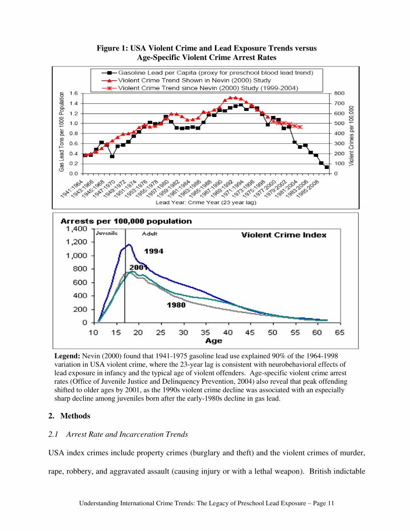
In a Supreme Court brief opposing juvenile executions, the American Psychological Association

(2004) argued that the adolescent brain “has not reached adult maturity, particularly in the frontal

lobes, which control … decision-making”. That brief included a graph showing violent offenses

“build steeply to 18, before starting to drop off” as offending is often “moderated or eliminated by

the individual in adulthood”. That same graph also reveals age-specific arrest rate shifts that track

lead exposure and violent crime trends [Figure 1]. Youths ages 16-22 in 1994 were all born

before the early-1980s fall in gasoline lead, and the age-16 arrest rate was 29% higher than the

age-22 rate in 1994, consistent with criminal behavior being moderated by changes in frontal lobe

development of adolescents and young adults. The 22-year-olds in 2001 were also born before the

early-1980s decline in lead exposure, but the 16-year-olds were born in the mid-1980s, and the

2001 age-16 arrest rate was 12% lower than the age-22 arrest rate.

This study examines international trends in preschool blood lead, crime rates, and age-specific

arrests rates, to test whether the relationship between lead exposure, arrest, and crime trends in

Figure 1 is evident across many crime categories and across nations with divergent preschool

blood lead and crime rate trends. International, racial, and city differences in severe lead

poisoning prevalence are also compared with subsequent contrasts in murder rates and juvenile

violence, with the expectation that severe preschool lead poisoning could be linked to more

violent offending and especially to murder rates.


Figure 1: USA Violent Crime and Lead Exposure Trends versus

Age-Specific Violent Crime Arrest Rates

Legend: Nevin (2000) found that 1941-1975 gasoline lead use explained 90% of the 1964-1998

variation in USA violent crime, where the 23-year lag is consistent with neurobehavioral effects of

lead exposure in infancy and the typical age of violent offenders. Age-specific violent crime arrest

rates (Office of Juvenile Justice and Delinquency Prevention, 2004) also reveal that peak offending

shifted to older ages by 2001, as the 1990s violent crime decline was associated with an especially

sharp decline among juveniles born after the early-1980s decline in gas lead.

2. Methods

2.1 Arrest Rate and Incarceration Trends

USA index crimes include property crimes (burglary and theft) and the violent crimes of murder,

rape, robbery, and aggravated assault (causing injury or with a lethal weapon). British indictable


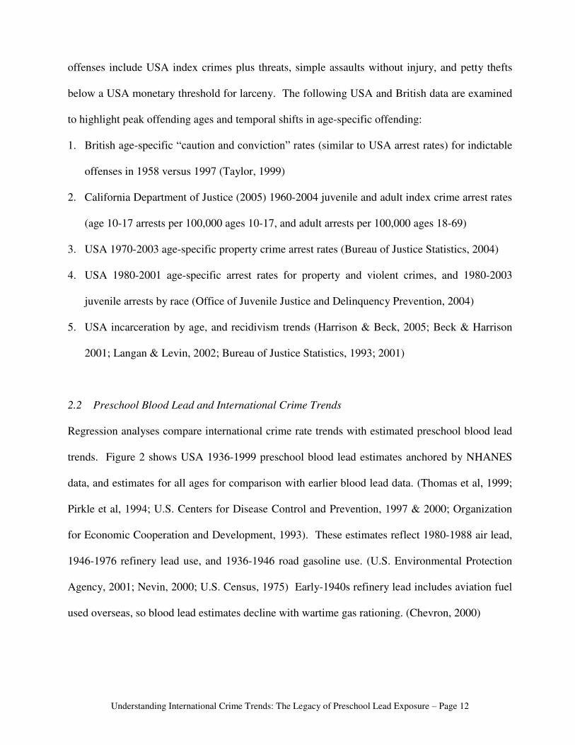
offenses include USA index crimes plus threats, simple assaults without injury, and petty thefts

below a USA monetary threshold for larceny. The following USA and British data are examined

to highlight peak offending ages and temporal shifts in age-specific offending:

1. British age-specific “caution and conviction” rates (similar to USA arrest rates) for indictable

offenses in 1958 versus 1997 (Taylor, 1999)

2. California Department of Justice (2005) 1960-2004 juvenile and adult index crime arrest rates

(age 10-17 arrests per 100,000 ages 10-17, and adult arrests per 100,000 ages 18-69)

3. USA 1970-2003 age-specific property crime arrest rates (Bureau of Justice Statistics, 2004)

4. USA 1980-2001 age-specific arrest rates for property and violent crimes, and 1980-2003

juvenile arrests by race (Office of Juvenile Justice and Delinquency Prevention, 2004)

5. USA incarceration by age, and recidivism trends (Harrison & Beck, 2005; Beck & Harrison

2001; Langan & Levin, 2002; Bureau of Justice Statistics, 1993; 2001)

2.2 Preschool Blood Lead and International Crime Trends

Regression analyses compare international crime rate trends with estimated preschool blood lead

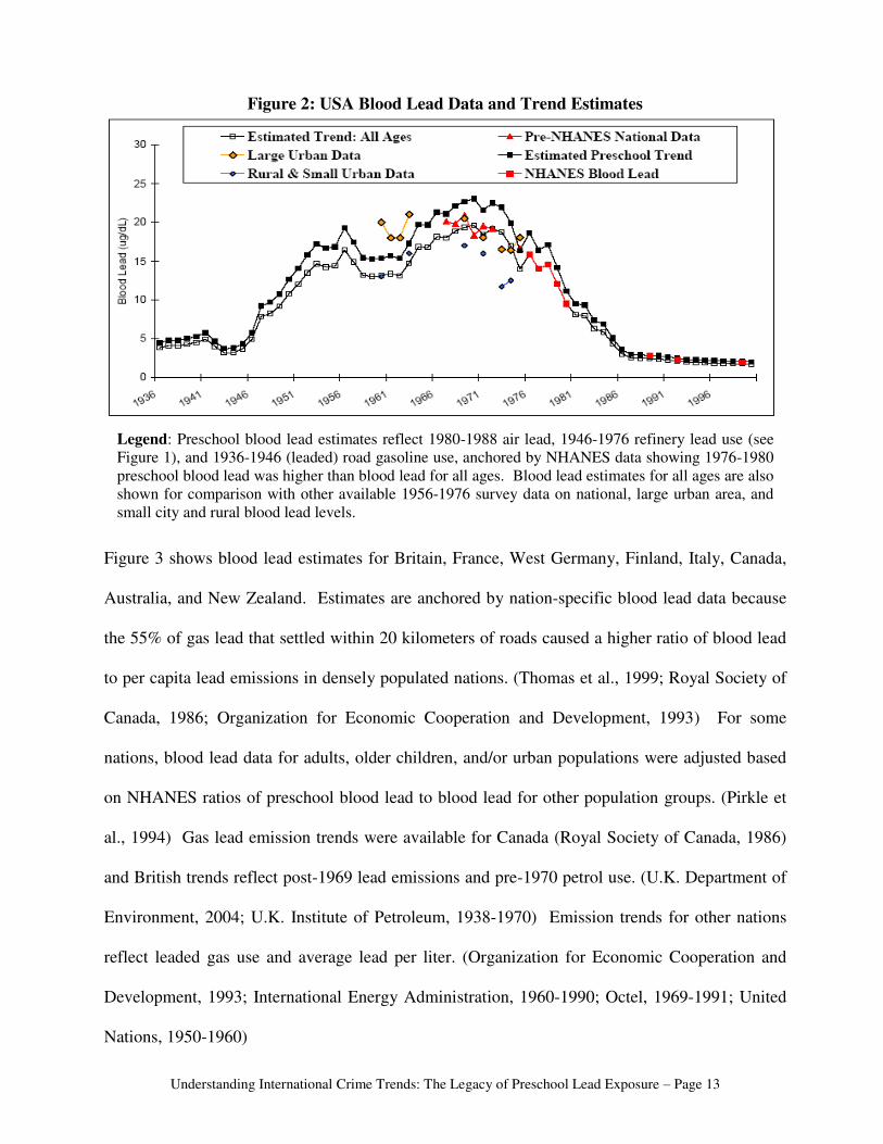
trends. Figure 2 shows USA 1936-1999 preschool blood lead estimates anchored by NHANES

data, and estimates for all ages for comparison with earlier blood lead data. (Thomas et al, 1999;

Pirkle et al, 1994; U.S. Centers for Disease Control and Prevention, 1997 & 2000; Organization

for Economic Cooperation and Development, 1993). These estimates reflect 1980-1988 air lead,

1946-1976 refinery lead use, and 1936-1946 road gasoline use. (U.S. Environmental Protection

Agency, 2001; Nevin, 2000; U.S. Census, 1975) Early-1940s refinery lead includes aviation fuel

used overseas, so blood lead estimates decline with wartime gas rationing. (Chevron, 2000)


Figure 2: USA Blood Lead Data and Trend Estimates

Legend: Preschool blood lead estimates reflect 1980-1988 air lead, 1946-1976 refinery lead use (see

Figure 1), and 1936-1946 (leaded) road gasoline use, anchored by NHANES data showing 1976-1980

preschool blood lead was higher than blood lead for all ages. Blood lead estimates for all ages are also

shown for comparison with other available 1956-1976 survey data on national, large urban area, and

small city and rural blood lead levels.

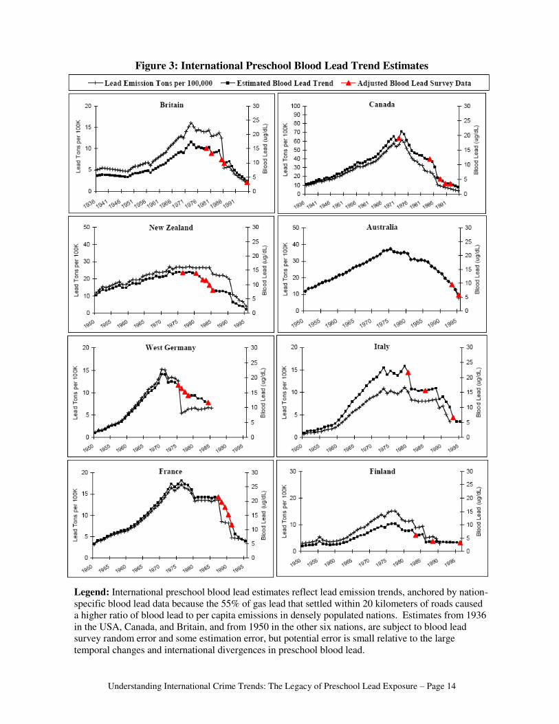
Figure 3 shows blood lead estimates for Britain, France, West Germany, Finland, Italy, Canada,

Australia, and New Zealand. Estimates are anchored by nation-specific blood lead data because

the 55% of gas lead that settled within 20 kilometers of roads caused a higher ratio of blood lead

to per capita lead emissions in densely populated nations. (Thomas et al., 1999; Royal Society of

Canada, 1986; Organization for Economic Cooperation and Development, 1993) For some

nations, blood lead data for adults, older children, and/or urban populations were adjusted based

on NHANES ratios of preschool blood lead to blood lead for other population groups. (Pirkle et

al., 1994) Gas lead emission trends were available for Canada (Royal Society of Canada, 1986)

and British trends reflect post-1969 lead emissions and pre-1970 petrol use. (U.K. Department of

Environment, 2004; U.K. Institute of Petroleum, 1938-1970) Emission trends for other nations

reflect leaded gas use and average lead per liter. (Organization for Economic Cooperation and

Development, 1993; International Energy Administration, 1960-1990; Octel, 1969-1991; United

Nations, 1950-1960)


Figure 3: International Preschool Blood Lead Trend Estimates

Legend: International preschool blood lead estimates reflect lead emission trends, anchored by nation-

specific blood lead data because the 55% of gas lead that settled within 20 kilometers of roads caused

a higher ratio of blood lead to per capita emissions in densely populated nations. Estimates from 1936

in the USA, Canada, and Britain, and from 1950 in the other six nations, are subject to blood lead

survey random error and some estimation error, but potential error is small relative to the large

temporal changes and international divergences in preschool blood lead.


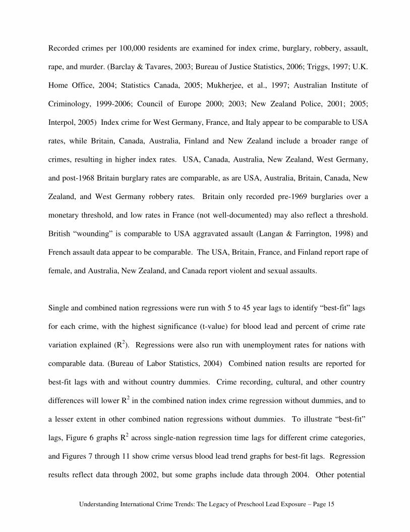
Recorded crimes per 100,000 residents are examined for index crime, burglary, robbery, assault,

rape, and murder. (Barclay & Tavares, 2003; Bureau of Justice Statistics, 2006; Triggs, 1997; U.K.

Home Office, 2004; Statistics Canada, 2005; Mukherjee, et al., 1997; Australian Institute of

Criminology, 1999-2006; Council of Europe 2000; 2003; New Zealand Police, 2001; 2005;

Interpol, 2005) Index crime for West Germany, France, and Italy appear to be comparable to USA

rates, while Britain, Canada, Australia, Finland and New Zealand include a broader range of

crimes, resulting in higher index rates. USA, Canada, Australia, New Zealand, West Germany,

and post-1968 Britain burglary rates are comparable, as are USA, Australia, Britain, Canada, New

Zealand, and West Germany robbery rates. Britain only recorded pre-1969 burglaries over a

monetary threshold, and low rates in France (not well-documented) may also reflect a threshold.

British “wounding” is comparable to USA aggravated assault (Langan & Farrington, 1998) and

French assault data appear to be comparable. The USA, Britain, France, and Finland report rape of

female, and Australia, New Zealand, and Canada report violent and sexual assaults.

Single and combined nation regressions were run with 5 to 45 year lags to identify “best-fit” lags

for each crime, with the highest significance (t-value) for blood lead and percent of crime rate

variation explained (R2). Regressions were also run with unemployment rates for nations with

comparable data. (Bureau of Labor Statistics, 2004) Combined nation results are reported for

best-fit lags with and without country dummies. Crime recording, cultural, and other country

differences will lower R2 in the combined nation index crime regression without dummies, and to

a lesser extent in other combined nation regressions without dummies. To illustrate “best-fit”

lags, Figure 6 graphs R2 across single-nation regression time lags for different crime categories,

and Figures 7 through 11 show crime versus blood lead trend graphs for best-fit lags. Regression

results reflect data through 2002, but some graphs include data through 2004. Other potential


confounders were excluded because preliminary analysis showed no impact on long-term crime

trends. The percent of USA violent crime involving guns was fairly stable from 1973-2004

(Bureau of Justice Statistics, 2005), as violent crime rose and fell sharply. Only 6% of murders in

1991 and 4% in 2001 were linked to drug offenses or brawls influenced by narcotics, and there

was little 1990s change in the percent of prisoners who committed crimes to get drug money

(Dorsey et al., 2005), as murder and other crimes fell sharply. International crime trends are

inconsistent with theoretical effects of police per capita, incarceration, and demographic trends.

(Barclay & Tavares, 2003; U.S. Census, 2004)

2.3 Cross-Sectional Regression Analysis of 1985-1994 USA Central City Murder Rates

A separate analysis compares average 1985-1994 murder rates across USA cities with differences

in circa-1970 lead paint poisoning and air lead exposure. Children under seven in 1970 were in

the high murder offense age bracket in 1985-1994. “LP%” values were constructed to estimate

the percent of each city’s 1985-1994 population that had severe childhood lead paint poisoning in

1970. City size dummy variables were used as indicators of 1970 air lead.

Gilsinn (1972) used population under seven and deteriorated and dilapidated housing prevalence

to estimate the number of children with blood lead over 40 ug/dL in each 1970 metro area. These

estimates approximate the number of central city children over 40 ug/dL because there was little

deteriorated housing in 1970 suburbs. Gilsinn’s estimates were divided by average 1985-1994

population for the corresponding cities to calculate LP%. Regression analysis compares LP%

with the average 1985-1994 murder rates in 124 central city/cities, including 11 combined city

murder rates calculated for metro areas with more than one central city. This regression does not

reflect air lead variations because Gilsinn’s estimates were based on housing data. A second


regression compares city murder rates with city size dummy variables as indicators of 1970 air

lead, using average 1985-1994 population and murder rates for the same 124 city/cities. A third

regression with LP% and city size dummies examines the additive effect of severe lead paint

hazards and air lead. The analysis also tests for the effect of the black percent of city population.

Limitations of this analysis include cities in the small size category with air lead affected by large

cities in another MSA (e.g., Newark and New York), children that moved between cities from

1970 to 1985-94, and 1970 city lead paint poisoning that is overstated to the extent that suburbs

did have some deteriorated housing (reflected in Gilsinn’s estimates).

3. Results


Age-14 British males had the highest caution and conviction rate for indictable offenses in 1958,

but peak offending shifted to age 18 by 1997. The age-10 offense rate fell 70% from 1958-1997,

as age 18-29 offending rates increased three to five fold. Males ages 12-14 in 1958, born as gas

lead exposure rose after World War II, had higher offending rates than older teens born before

that rise in lead exposure. By 1997, offending declined relative to 1958 only for males under 14,

born after the mid-1980s fall in British gas lead use, while offending rates rose for older teens and

adults born over years of rising gasoline lead use.

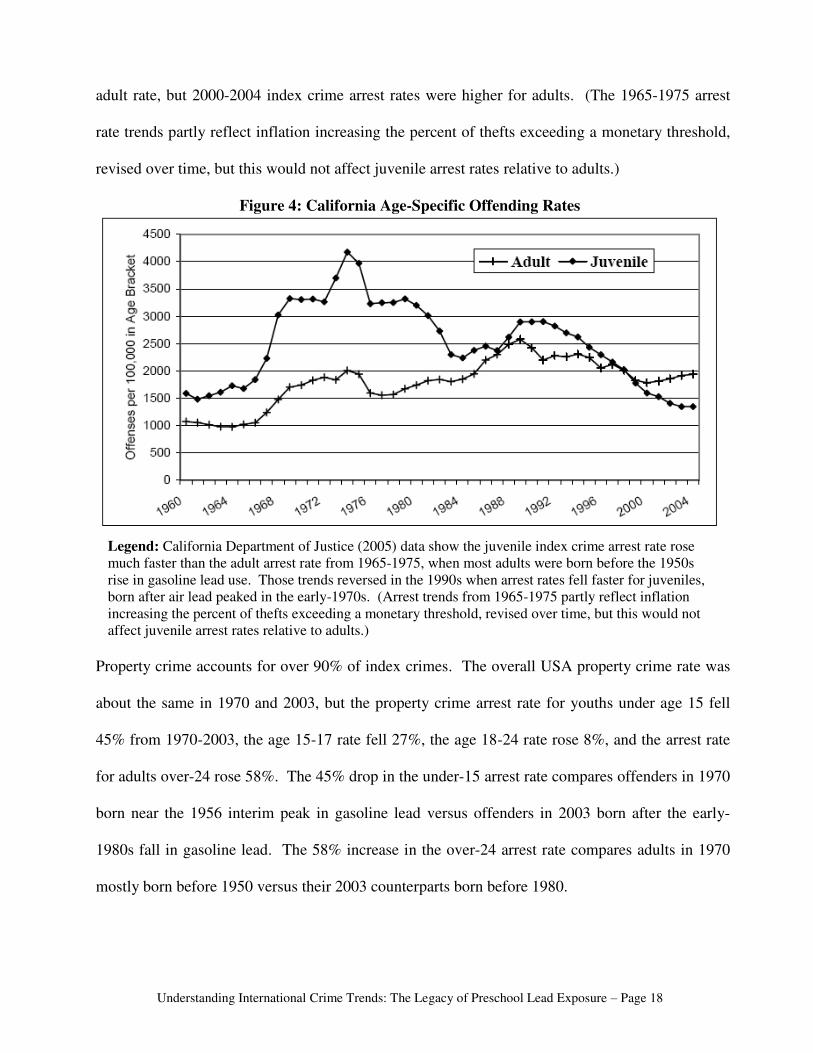
USA per capita gasoline lead increased 400% from 1945-55, and Figure 4 shows the California

juvenile index crime arrest rate surged almost 300% from 1965 to 1975. The adult arrest rate rose

at a much slower rate, when most adults were born before the 1950s surge in gasoline lead use.

Those trends reversed in the 1990s when arrest rates fell faster for juveniles, born after air lead

peaked in the early-1970s. In 1975, California’s juvenile index crime arrest rate was twice the


adult rate, but 2000-2004 index crime arrest rates were higher for adults. (The 1965-1975 arrest

rate trends partly reflect inflation increasing the percent of thefts exceeding a monetary threshold,

revised over time, but this would not affect juvenile arrest rates relative to adults.)

Figure 4: California Age-Specific Offending Rates

Legend: California Department of Justice (2005) data show the juvenile index crime arrest rate rose

much faster than the adult arrest rate from 1965-1975, when most adults were born before the 1950s

rise in gasoline lead use. Those trends reversed in the 1990s when arrest rates fell faster for juveniles,

born after air lead peaked in the early-1970s. (Arrest trends from 1965-1975 partly reflect inflation

increasing the percent of thefts exceeding a monetary threshold, revised over time, but this would not

affect juvenile arrest rates relative to adults.)

Property crime accounts for over 90% of index crimes. The overall USA property crime rate was

about the same in 1970 and 2003, but the property crime arrest rate for youths under age 15 fell

45% from 1970-2003, the age 15-17 rate fell 27%, the age 18-24 rate rose 8%, and the arrest rate

for adults over-24 rose 58%. The 45% drop in the under-15 arrest rate compares offenders in 1970

born near the 1956 interim peak in gasoline lead versus offenders in 2003 born after the early-

1980s fall in gasoline lead. The 58% increase in the over-24 arrest rate compares adults in 1970

mostly born before 1950 versus their 2003 counterparts born before 1980.


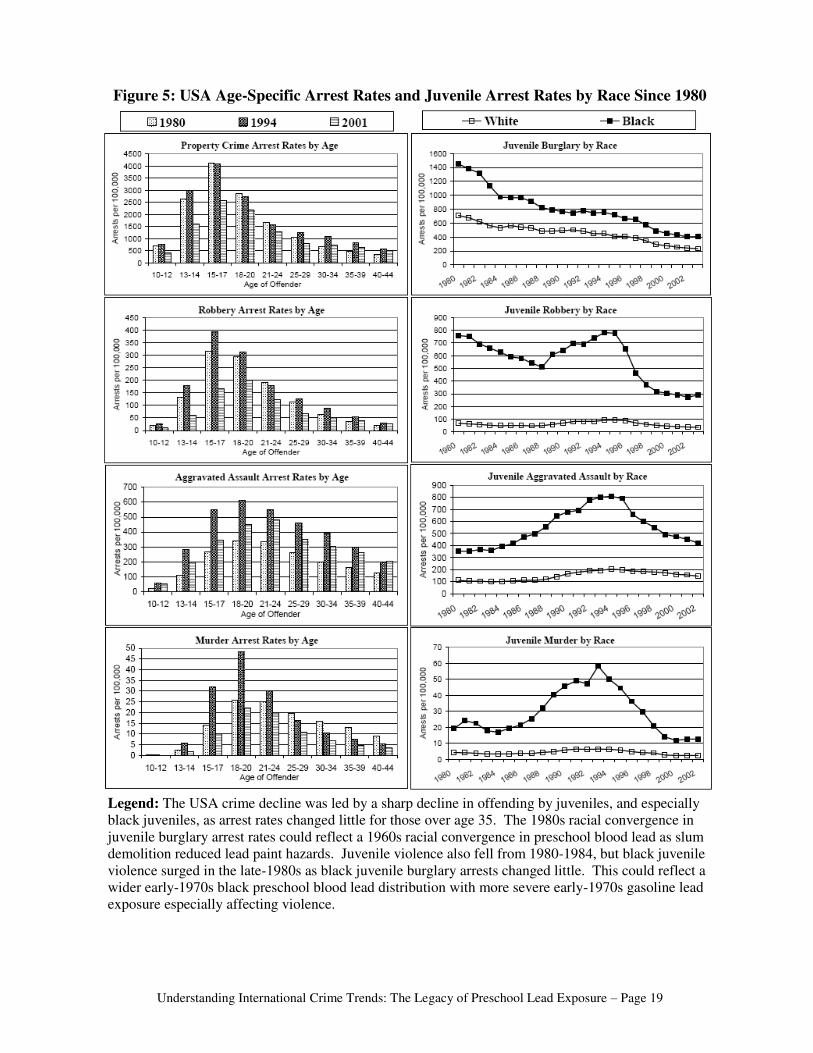
Figure 5: USA Age-Specific Arrest Rates and Juvenile Arrest Rates by Race Since 1980

Legend: The USA crime decline was led by a sharp decline in offending by juveniles, and especially

black juveniles, as arrest rates changed little for those over age 35. The 1980s racial convergence in

juvenile burglary arrest rates could reflect a 1960s racial convergence in preschool blood lead as slum

demolition reduced lead paint hazards. Juvenile violence also fell from 1980-1984, but black juvenile

violence surged in the late-1980s as black juvenile burglary arrests changed little. This could reflect a

wider early-1970s black preschool blood lead distribution with more severe early-1970s gasoline lead

exposure especially affecting violence.


Figure 5 compares 1980-2001 age-specific USA arrest rates and 1980-2003 juvenile arrest rates

by race. The 1980-2001 USA property crime decline was led by a 70% fall in the black juvenile

burglary arrest rate, which fell much faster than the white juvenile arrest rate from 1980-1988,

narrowing the racial difference. Juvenile burglary rates were little changed from 1988-1994, but

fell further after 1994. The 2003 black juvenile burglary arrest rate was 43% below the 1980

white juvenile rate. Peak offending for robbery is a few years older than for propety crime, and

the 42% fall in the robbery rate from 1980-2001 was entirely due to sharply lower arrest rates for

juveniles and young adults, as the age 35-44 arrest rate rose. The black juvenile robbery arrest

rate fell from 1980-1988, narrowing the racial difference, but the black rate and racial difference

rose from 1988-1994 before falling to new lows in 2001-2003. Aggravated assault offending

peaks at an older age than robbery and falls more slowly with age. Aggravated assault arrests

rose for all ages from 1980-1994, but the age 40-44 arrest rate continued to rise through 2001.

Black juveniles recorded the largest rise from 1985-1994, and the sharpest fall from 1994-2001.

The under-21 homicide arrest rate soared from 1984-1994 as the over-25 rate declined, but the

1990s homicide rate decline was mainly due to a sharp fall in the under-21 rate. The black

juvenile murder arrest rate drifted lower in the early-1980s then rose sharply before falling to

multi-decade lows. The racial difference in juvenile murder arrest rates peaked in 1994, but the

2003 difference was only about one-fourth the average racial difference from 1980-1998.

USA incarceration trends echo arrest trends, as offenders over age 34 accounted for just 27% of

prison commitments in 1993 but accounted for 40% in 2001. The overall USA incarceration rate

changed little from 2000-2004, but the age 18-19 male incarceration rate fell 30% and the age 20-

34 rate fell 7%, as the male incarceration rate rose 5% for ages 35-39, 21% for ages 40-44, 26%

for ages 45-54, and 41% for those over 55. Over 60% of prisoners released in both 1983 and


1994 were rearrested within three years, but 35% of those released in 1983 were ages 18-25

versus 21% in 1994. Combining prisoner release trends with recidivist offending rates suggests

that prisoners released in the prior three years committed just 6% of property crimes and 11% of

violent crimes in 1979 versus 28% of property crimes and 35% of violent crimes in 2002.

3.2 Preschool Blood Lead and International Crime Trend Regressions

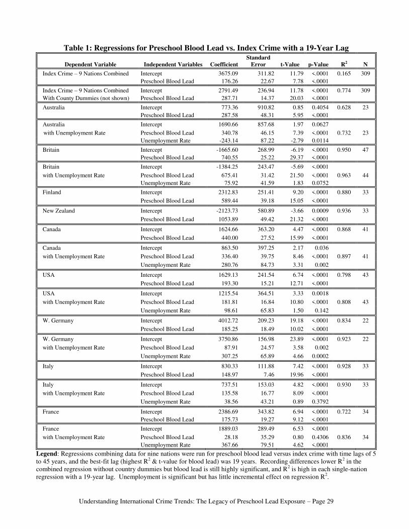
The best-fit time lag for index crime versus preschool blood lead is 19 years in a regression with

country dummies comparing 309 years of data across nine nations. The same best-fit time lag is

evident in single-nation regressions with and without an unemployment variable. Table 1 shows

regression results with a 19-year lag, Figure 6 graphs R2 across lags for each nation, and Figures 7

& 8 graph preschool blood lead trends versus index crime rates with a 19-year lag. Blood lead is

highly significant in combined and single-nation regressions with and without country dummies.

Unemployment is significant in most nations but its inclusion in the model has no substantive

effect on the blood lead coefficient value or significance (t-value), and little impact on crime rate

variation explained (R2). Adding unemployment raises R

2 from: 80% to 81% for the USA; 87%

to 90% for Canada; 72% to 84% for France; and 83% to 92% for West Germany. Italy and

Britain R2 with just blood lead is 93% to 95% and unemployment is insignificant. Graphs across

time lags show R2 (and blood lead t-value) peaks at 18 to 21 years in six nations, at 14-15 years in

West Germany (N=22) and France (N=33) and 26 years in Australia (N=23).

The best-fit lag for burglary is 18 years in a combined regression for eight nations (N=229) with

country dummies, and for five nations (N=169) with unemployment data (excluding burglary data

for France suggesting a monetary threshold). Table 2 shows blood lead is highly significant in

combined and single-nation burglary regressions. Figure 6 shows R2 across time lags for each


nation, and Figure 9 graphs burglary versus blood lead with an 18-year lag. Unemployment is

significant but its inclusion only increases R2 from 65% to 73% for the USA; 78% to 86% for

Canada; 85% to 88% for Britain; and 82% to 92% for West Germany. Australia R2 is 91% with

just blood lead (unemployment is insignificant) and New Zealand R2 is 86% with just blood lead.

R2 peaks at lags of 16-19 years in seven nations, and 21 years in Australia, based on data through

2002. Australia’s burglary rate fell about 20% from 2002-2004.

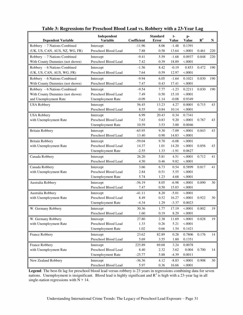
The best-fit lag for robbery across seven nations (N=220) is 23 years, and unemployment is

insignificant across six nations (N=190). Table 3 shows blood lead with a 23-year lag is highly

significant in combined and single-nation regressions. Figure 10 graphs robbery versus blood

lead with a 23-year lag. Adding unemployment raises R2 somewhat for the USA and Canada but

unemployment is insignificant or has an unexpected sign in other nations. The best fit is 20-21

years in four nations, 36 years in France (N=14) and 26-28 in Britain and Australia through 2002.

Britain and Australia robbery rates fell about 20% from 2002-2004.

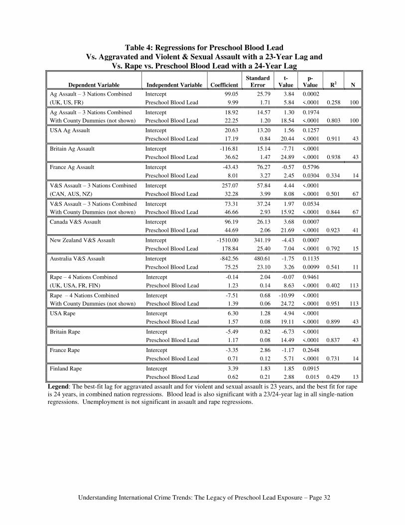
Table 4 and Figure 11 show blood lead with a 23-year lag is highly significant in regressions for

aggravated assault (N=100) and violent and sexual assault (N=67), and with a 24-year lag for rape

(N=113). Unemployment is insignificant. The best-fit for aggravated assault is 24 years in the

USA (N=43), 23 in Britain (N=43), and 29-33 years in France (N=14). The best fit lag for violent

and sexual assault is 24 years in Canada (N=41), 22 in New Zealand (N=15), and 28-33 in

Australia (N=11). The best-fit for rape is 23 years in the USA (N=43), 30 in Britain (N=43), 29

in France (N=14), and 27-33 in Finland (N=13). Figure 6 shows regression R2 for aggravated

assault, violent and sexual assault, and rape reach absolute peaks across a range of longer lags in

single-nation regressions. However, Table 4 shows R2 and t-values are very high with the 23-24


year time lag for all single-nation regressions with over 14 years of data (R2 of 79% to 94%).

Table 5 shows blood lead with an 18-year lag is significant in the combined nation murder

regression (N=209) and unemployment is insignificant (N=178). The best-fit time lag is 18-19

years for the USA, New Zealand, and Britain, but Canada has a shorter best-fit and average

preschool blood lead is not significant in murder regressions for Australia or West Germany.

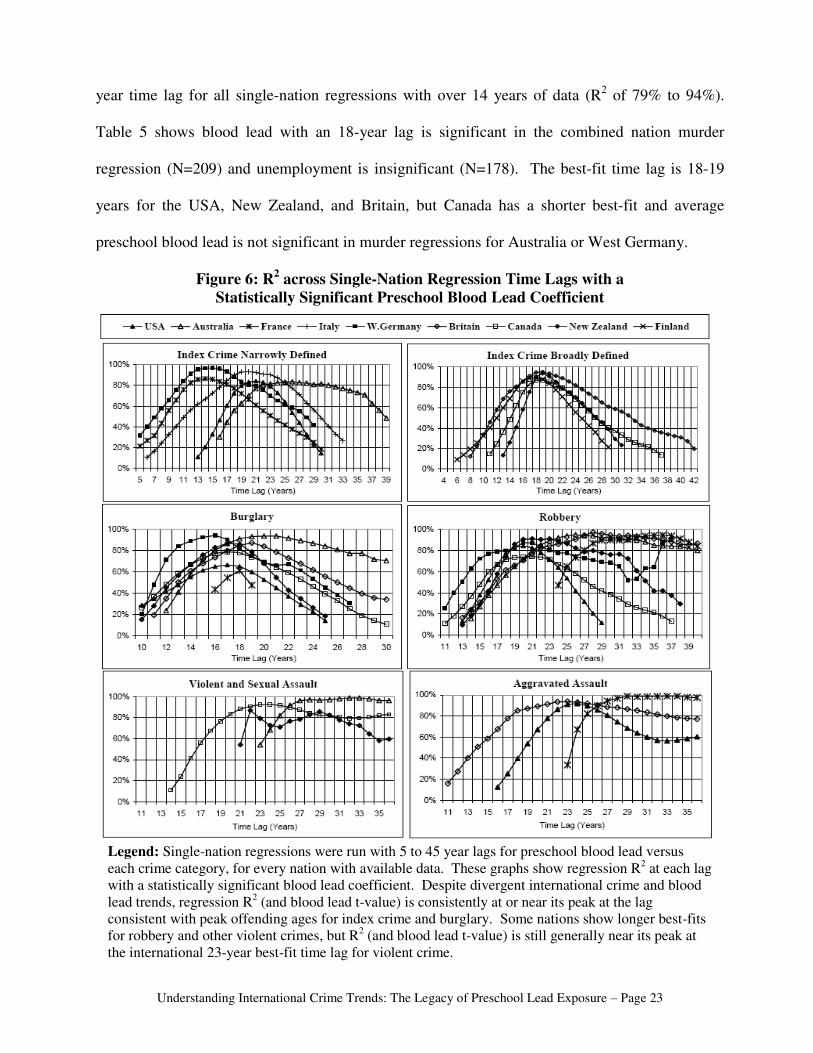
Figure 6: R2 across Single-Nation Regression Time Lags with a

Statistically Significant Preschool Blood Lead Coefficient

Legend: Single-nation regressions were run with 5 to 45 year lags for preschool blood lead versus

each crime category, for every nation with available data. These graphs show regression R2 at each lag

with a statistically significant blood lead coefficient. Despite divergent international crime and blood

lead trends, regression R2 (and blood lead t-value) is consistently at or near its peak at the lag

consistent with peak offending ages for index crime and burglary. Some nations show longer best-fits

for robbery and other violent crimes, but R2 (and blood lead t-value) is still generally near its peak at

the international 23-year best-fit time lag for violent crime.


Figure 7: Preschool Blood Lead vs. Narrowly Defined Index Crime with a 19-Year Lag

Legend: These graphs show preschool blood lead trends versus narrowly defined index crime rates

with a 19-year lag. USA index crime includes property crimes (theft and burglary) and the violent

crimes of murder, rape, robbery, and aggravated assault (causing injury or with a lethal weapon).

Nations with comparable crime indexes all show index crime rates tracking preschool blood lead

trends with a 19 year lag, despite divergent crime trends. The USA index crime rate was 22% higher

than the French rate and 40% higher than Australia’s rate in 1980, but the USA rate was 39% below

the French rate and 45% below Australia’s rate in 2001.


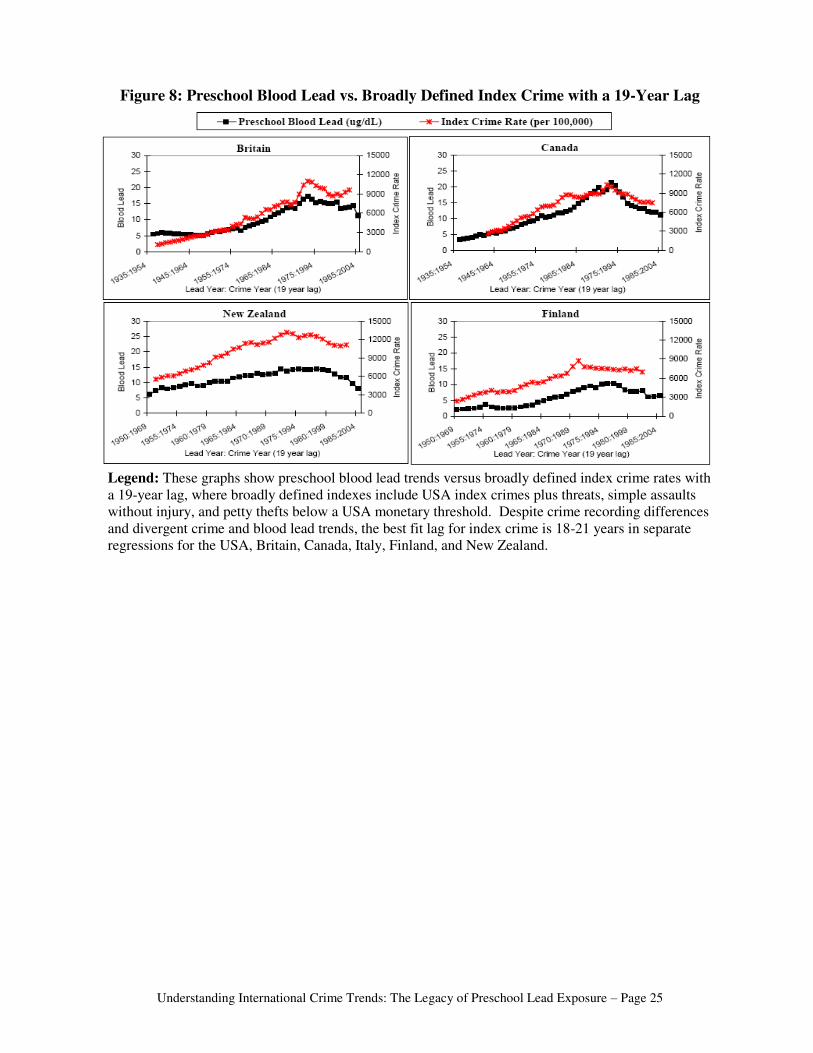
Figure 8: Preschool Blood Lead vs. Broadly Defined Index Crime with a 19-Year Lag

Legend: These graphs show preschool blood lead trends versus broadly defined index crime rates with

a 19-year lag, where broadly defined indexes include USA index crimes plus threats, simple assaults

without injury, and petty thefts below a USA monetary threshold. Despite crime recording differences

and divergent crime and blood lead trends, the best fit lag for index crime is 18-21 years in separate

regressions for the USA, Britain, Canada, Italy, Finland, and New Zealand.


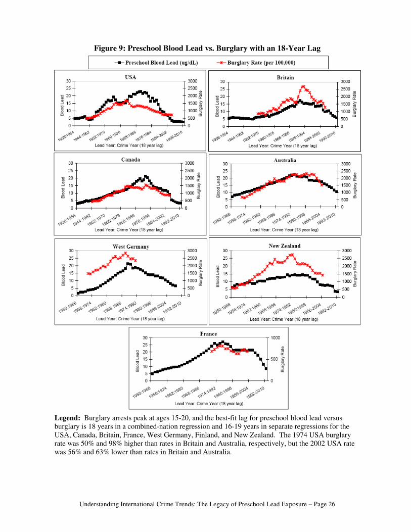
Figure 9: Preschool Blood Lead vs. Burglary with an 18-Year Lag

Legend: Burglary arrests peak at ages 15-20, and the best-fit lag for preschool blood lead versus

burglary is 18 years in a combined-nation regression and 16-19 years in separate regressions for the

USA, Canada, Britain, France, West Germany, Finland, and New Zealand. The 1974 USA burglary

rate was 50% and 98% higher than rates in Britain and Australia, respectively, but the 2002 USA rate

was 56% and 63% lower than rates in Britain and Australia.


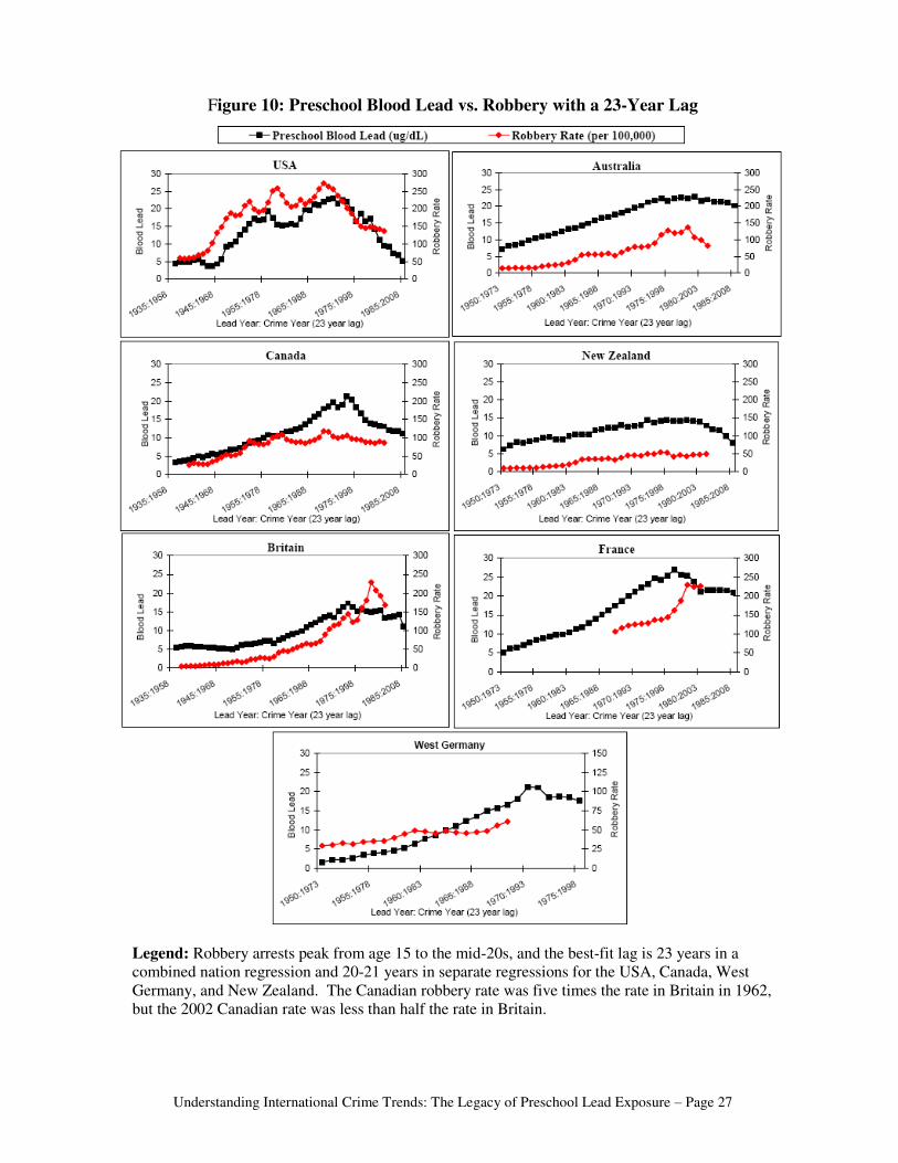
Figure 10: Preschool Blood Lead vs. Robbery with a 23-Year Lag

Legend: Robbery arrests peak from age 15 to the mid-20s, and the best-fit lag is 23 years in a

combined nation regression and 20-21 years in separate regressions for the USA, Canada, West

Germany, and New Zealand. The Canadian robbery rate was five times the rate in Britain in 1962,

but the 2002 Canadian rate was less than half the rate in Britain.


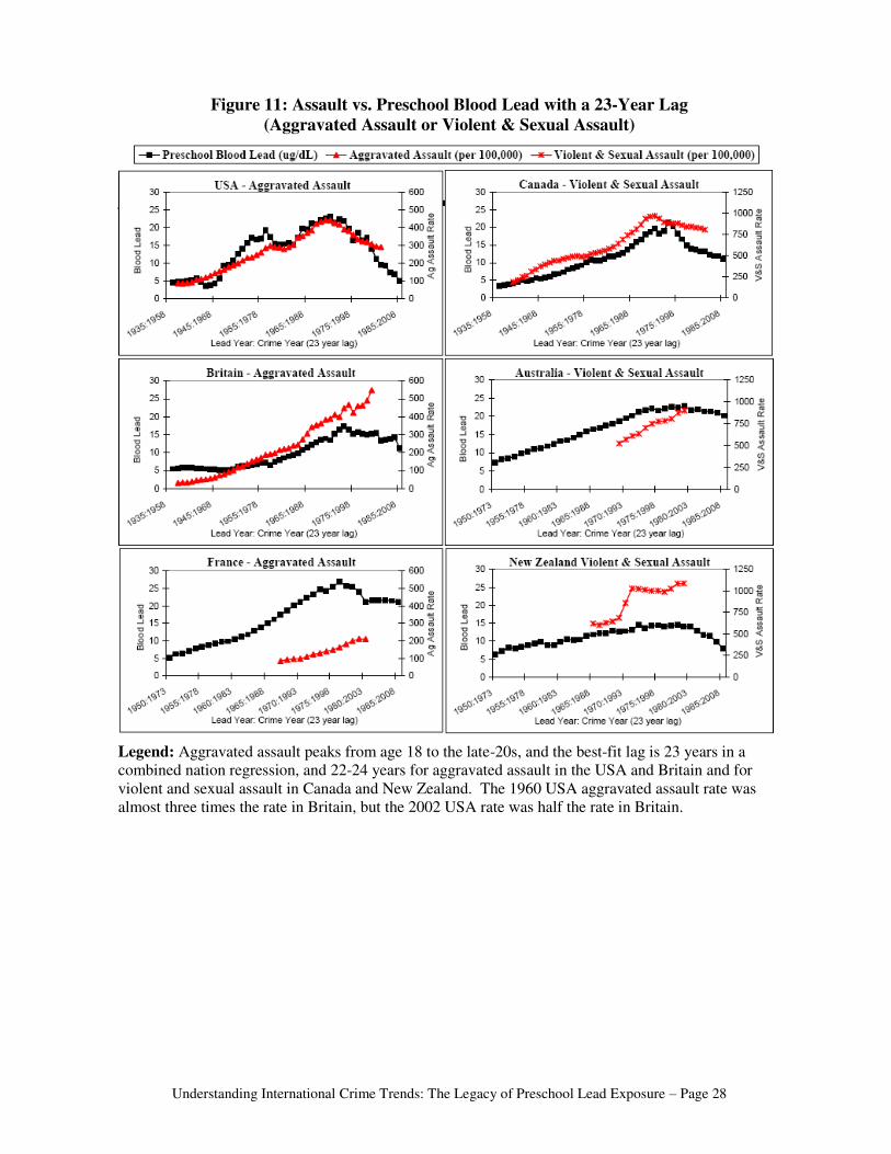
Figure 11: Assault vs. Preschool Blood Lead with a 23-Year Lag

(Aggravated Assault or Violent & Sexual Assault)

Legend: Aggravated assault peaks from age 18 to the late-20s, and the best-fit lag is 23 years in a

combined nation regression, and 22-24 years for aggravated assault in the USA and Britain and for

violent and sexual assault in Canada and New Zealand. The 1960 USA aggravated assault rate was

almost three times the rate in Britain, but the 2002 USA rate was half the rate in Britain.


Table 1: Regressions for Preschool Blood Lead vs. Index Crime with a 19-Year Lag

Dependent Variable Independent Variables Coefficient

Standard

Error t-Value p-Value R2 N

Index Crime – 9 Nations Combined Intercept 3675.09 311.82 11.79 <.0001 0.165 309

Preschool Blood Lead 176.26 22.67 7.78 <.0001

Index Crime – 9 Nations Combined Intercept 2791.49 236.94 11.78 <.0001 0.774 309

With County Dummies (not shown) Preschool Blood Lead 287.71 14.37 20.03 <.0001

Australia Intercept 773.36 910.82 0.85 0.4054 0.628 23


Australia Intercept 1690.66 857.68 1.97 0.0627

with Unemployment Rate Preschool Blood Lead 340.78 46.15 7.39 <.0001 0.732 23

Unemployment Rate -243.14 87.22 -2.79 0.0114

Britain Intercept -1665.60 268.99 -6.19 <.0001 0.950 47


Britain Intercept -1384.25 243.47 -5.69 <.0001


Unemployment Rate 75.92 41.59 1.83 0.0752

Finland Intercept 2312.83 251.41 9.20 <.0001 0.880 33


New Zealand Intercept -2123.73 580.89 -3.66 0.0009 0.936 33


Canada Intercept 1624.66 363.20 4.47 <.0001 0.868 41


Canada Intercept 863.50 397.25 2.17 0.036



USA Intercept 1629.13 241.54 6.74 <.0001 0.798 43


USA Intercept 1215.54 364.51 3.33 0.0018



W. Germany Intercept 4012.72 209.23 19.18 <.0001 0.834 22


W. Germany Intercept 3750.86 156.98 23.89 <.0001 0.923 22

with Unemployment Rate Preschool Blood Lead 87.91 24.57 3.58 0.002


Italy Intercept 830.33 111.88 7.42 <.0001 0.928 33


Italy Intercept 737.51 153.03 4.82 <.0001 0.930 33

with Unemployment Rate Preschool Blood Lead 135.58 16.77 8.09 <.0001


France Intercept 2386.69 343.82 6.94 <.0001 0.722 34


France Intercept 1889.03 289.49 6.53 <.0001

with Unemployment Rate Preschool Blood Lead 28.18 35.29 0.80 0.4306 0.836 34

Unemployment Rate 367.66 79.51 4.62 <.0001

Legend: Regressions combining data for nine nations were run for preschool blood lead versus index crime with time lags of 5

to 45 years, and the best-fit lag (highest R2 & t-value for blood lead) was 19 years. Recording differences lower R

2 in the

combined regression without country dummies but blood lead is still highly significant, and R2 is high in each single-nation

regression with a 19-year lag. Unemployment is significant but has little incremental effect on regression R2.


Table 2: Regressions for Preschool Blood Lead vs. Burglary with an 18-Year Lag

Dependent Variable

Independent

Variable Coefficient

Standard

Error

t-

Value

p-

Value R2 N

Burglary – 8 Nations Combined Intercept 1072.11 106.53 10.06 <.0001 0.060 229

(UK, US, CAN, AUS, NZ, WG, FR, FIN) Preschool Blood Lead 27.63 7.23 3.82 0.0002




(UK, US, CAN, AUS, WG) Preschool Blood Lead 61.76 7.32 8.44 <.0001





and Unemployment Rate Unemployment Rate 78.91 9.96 7.92 <.0001

USA Burglary Intercept 397.67 84.11 4.73 <.0001 0.653 43


USA Burglary Intercept 112.06 115.39 0.97 0.3373



Britain Burglary Intercept -51.84 129.15 -0.40 0.6908 0.849 34


Britain Burglary Intercept -147.83 119.74 -1.23 0.2263 0.883 34



Canada Burglary Intercept 245.40 75.37 3.26 0.0023 0.781 41


Canada Burglary Intercept 69.76 72.04 0.97 0.339 0.860 41



Australia Burglary Intercept -544.87 133.16 -4.09 0.0003 0.912 31


Australia Burglary Intercept -538.67 133.18 -4.04 0.0004



W. Germany Burglary Intercept 1403.17 95.86 14.64 <.0001 0.819 20


W. Germany Burglary Intercept 1274.62 69.79 18.26 <.0001 0.923 20

with Unemployment Rate Preschool Blood Lead 31.58 8.59 3.67 0.0019


France Burglary Intercept 261.69 105.51 2.48 0.0289 0.614 14

Preschool Blood Lead 19.31 4.42 4.36 0.0009

France Burglary Intercept 272.37 114.21 2.38 0.0362



Finland Burglary Intercept 1065.13 378.40 2.81 0.0202 0.286 11


New Zealand Burglary Intercept -1153.40 205.29 -5.62 <.0001 0.862 35


Legend: Combined-nation regressions for preschool blood lead versus burglary with time lags of 5 to 45 years showed a

best-fit lag of 18 years (comparing 229 years of data across eight nations). Blood lead is also highly significant and R2 is

high with an 18-year lag in all single-nation regressions with N > 11. Unemployment is statistically significant but has

little incremental effect on regression R2.


Table 3: Regressions for Preschool Blood Lead vs. Robbery with a 23-Year Lag

Dependent Variable

Independent


Standard

Error

t-

Value

p-

Value R2 N

Robbery – 7 Nations Combined Intercept -11.96 8.06 -1.48 0.1391

(UK, US, CAN, AUS, NZ, WG, FR) Preschool Blood Lead 7.88 0.58 13.64 <.0001 0.461 220

Robbery – 7 Nations Combined Intercept -9.41 5.59 -1.68 0.0937 0.848 220



(UK, US, CAN, AUS, WG, FR) Preschool Blood Lead 7.64 0.59 12.97 <.0001





and Unemployment Rate Unemployment Rate -0.09 1.14 -0.08 0.9349

USA Robbery Intercept 56.45 13.23 4.27 0.0001 0.715 43


USA Robbery Intercept 6.99 20.43 0.34 0.7341



Britain Robbery Intercept -65.95 9.30 -7.09 <.0001 0.843 43


Britain Robbery Intercept -59.04 9.70 -6.08 <.0001



Canada Robbery Intercept 26.20 5.81 4.51 <.0001 0.712 41


Canada Robbery Intercept 3.66 6.73 0.54 0.5899 0.817 41



Australia Robbery Intercept -56.19 8.05 -6.98 <.0001 0.890 30


Australia Robbery Intercept -41.11 8.20 -5.01 <.0001



W. Germany Robbery Intercept 30.36 1.77 17.19 <.0001 0.802 19


W. Germany Robbery Intercept 27.80 2.38 11.69 <.0001 0.828 19



France Robbery Intercept 23.62 82.89 0.28 0.7806 0.176 14


France Robbery Intercept 225.89 69.68 3.24 0.0078



New Zealand Robbery Intercept -36.36 4.12 -8.83 <.0001 0.908 30


Legend: The best-fit lag for preschool blood lead versus robbery is 23 years in regressions combining data for seven

nations. Unemployment is insignificant. Blood lead is highly significant and R2 is high with a 23-year lag in all

single-nation regressions with N > 14.


Table 4: Regressions for Preschool Blood Lead

Vs. Aggravated and Violent & Sexual Assault with a 23-Year Lag and

Vs. Rape vs. Preschool Blood Lead with a 24-Year Lag

Dependent Variable Independent Variable Coefficient

Standard

Error

t-

Value

p-

Value R2 N

Ag Assault – 3 Nations Combined Intercept 99.05 25.79 3.84 0.0002

(UK, US, FR) Preschool Blood Lead 9.99 1.71 5.84 <.0001 0.258 100

Ag Assault – 3 Nations Combined Intercept 18.92 14.57 1.30 0.1974

With County Dummies (not shown) Preschool Blood Lead 22.25 1.20 18.54 <.0001 0.803 100

USA Ag Assault Intercept 20.63 13.20 1.56 0.1257

Preschool Blood Lead 17.19 0.84 20.44 <.0001 0.911 43

Britain Ag Assault Intercept -116.81 15.14 -7.71 <.0001


France Ag Assault Intercept -43.43 76.27 -0.57 0.5796

Preschool Blood Lead 8.01 3.27 2.45 0.0304 0.334 14

V&S Assault – 3 Nations Combined Intercept 257.07 57.84 4.44 <.0001

(CAN, AUS, NZ) Preschool Blood Lead 32.28 3.99 8.08 <.0001 0.501 67

V&S Assault – 3 Nations Combined Intercept 73.31 37.24 1.97 0.0534


Canada V&S Assault Intercept 96.19 26.13 3.68 0.0007


New Zealand V&S Assault Intercept -1510.00 341.19 -4.43 0.0007


Australia V&S Assault Intercept -842.56 480.61 -1.75 0.1135


Rape – 4 Nations Combined Intercept -0.14 2.04 -0.07 0.9461

(UK, USA, FR, FIN) Preschool Blood Lead 1.23 0.14 8.63 <.0001 0.402 113

Rape – 4 Nations Combined Intercept -7.51 0.68 -10.99 <.0001


USA Rape Intercept 6.30 1.28 4.94 <.0001


Britain Rape Intercept -5.49 0.82 -6.73 <.0001


France Rape Intercept -3.35 2.86 -1.17 0.2648


Finland Rape Intercept 3.39 1.83 1.85 0.0915


Legend: The best-fit lag for aggravated assault and for violent and sexual assault is 23 years, and the best fit for rape

is 24 years, in combined nation regressions. Blood lead is also significant with a 23/24-year lag in all single-nation

regressions. Unemployment is not significant in assault and rape regressions.


Table 5: Regressions for Murder vs. Preschool Blood Lead with an 18-Year Lag

Dependent Variable

Independent


Standard

Error

t-

Value

p-

Value R2 N

Murder – 6 Nations Combined Intercept 0.523 0.468 1.12 0.265

(UK, US, CAN, AUS, NZ, WG) Preschool Blood Lead 0.192 0.034 5.73 <.0001 0.137 209

Rape – 6 Nations Combined Intercept -0.052 0.160 -0.32 0.7471


USA Murder Intercept 3.827 0.401 9.54 <.0001


USA Murder Intercept 2.954 0.592 4.99 <.0001



Britain Murder Intercept 0.458 0.064 7.21 <.0001


Britain Murder Intercept 0.461 0.064 7.17 <.0001



Canada Murder Intercept 1.280 0.186 6.90 <.0001


Canada Murder Intercept 1.010 0.205 4.92 <.0001



Australia Murder Intercept 2.290 0.159 14.44 <.0001

Preschool Blood Lead -0.020 0.009 -2.21 0.035 0.144 31

Australia Murder Intercept 2.302 0.154 14.98 <.0001

with Unemployment Rate Preschool Blood Lead -0.040 0.015 -2.74 0.0105 0.226 31


West German Murder Intercept 1.361 0.052 26.27 <.0001


West German Murder Intercept 1.307 0.047 27.93 <.0001

with Unemployment Rate Preschool Blood Lead -0.012 0.006 -2.03 0.0588 0.358 20


New Zealand Murder Intercept -0.583 0.505 -1.15 0.2575


Legend: The best-fit lag for murder is 18 years in regressions combining data across six nations. Unemployment is

insignificant. Blood lead is not significant or has an unexpected sign in murder regressions for Australia and West

Germany, but blood lead is highly significant in other single-nation regressions for murder with an 18-year lag.

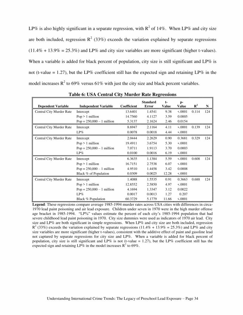
3.3 Cross-Sectional Regression Analysis of 1985-1994 USA Central City Murder Rates

Table 6 shows the regression analyses of 1985-1994 average murder rates across 124 central

city/cities. The average 1985-1994 murder rate was 33 (per 100,000) in central city/cities with

population over a million, 21 in cities of 250,000 to one million, and 15 in cities of 100-250

thousand, and city size dummy variables are significant in a simple regression, with R2 of 11.4%.


LP% is also highly significant in a separate regression, with R2 of 14%. When LP% and city size

are both included, regression R2 (33%) exceeds the variation explained by separate regressions

(11.4% + 13.9% = 25.3%) and LP% and city size variables are more significant (higher t-values).

When a variable is added for black percent of population, city size is still significant and LP% is

not (t-value = 1.27), but the LP% coefficient still has the expected sign and retaining LP% in the

model increases R2 to 69% versus 61% with just the city size and black percent variables.

Table 6: USA Central City Murder Rate Regressions

Dependent Variable Independent Variable Coefficient

Standard

Error

t-

Value

p-

Value R2 N

Central City Murder Rate Intercept 13.6401 1.4541 9.38 <.0001 0.114 124

Pop > 1 million 14.7560 4.1127 3.59 0.0005

Pop = 250,000 – 1 million 5.3137 2.1624 2.46 0.0154


LP% 0.0078 0.0018 4.44 <.0001

Central City Murder Rate Intercept 2.0444 2.2629 0.90 0.3681 0.329 124

Pop > 1 million 19.4911 3.6754 5.30 <.0001

Pop = 250,000 – 1 million 7.0711 1.9113 3.70 0.0003

LP% 0.0100 0.0016 6.19 <.0001


Pop > 1 million 16.7151 2.7538 6.07 <.0001

Pop = 250,000 – 1 million 4.9510 1.4458 3.42 0.0008

Black % of Population 0.0309 0.0025 12.28 <.0001

Central City Murder Rate Intercept 1.4088 1.5535 0.91 0.3663 0.688 124

Pop > 1 million 12.8552 2.5850 4.97 <.0001

Pop = 250,000 – 1 million 4.1694 1.3347 3.12 0.0022

LP% 0.0017 0.0013 1.27 0.207

Black % Population 60.3729 5.1779 11.66 <.0001

Legend: These regressions compare average 1985-1994 murder rates across USA cities with differences in circa-

1970 lead paint poisoning and air lead exposure. Children under seven in 1970 were in the high murder offense

age bracket in 1985-1994. “LP%” values estimate the percent of each city’s 1985-1994 population that had

severe childhood lead paint poisoning in 1970. City size dummies were used as indicators of 1970 air lead. City

size and LP% are both significant in simple regressions. When LP% and city size are both included, regression

R2 (33%) exceeds the variation explained by separate regressions (11.4% + 13.9% = 25.3%) and LP% and city

size variables are more significant (higher t-values), consistent with the additive effect of paint and gasoline lead

not captured by separate regressions for city size and LP%. When a variable is added for black percent of

population, city size is still significant and LP% is not (t-value = 1.27), but the LP% coefficient still has the

expected sign and retaining LP% in the model increases R2 to 69%.


4. Discussion


The 1980s racial convergence in juvenile burglary rates could reflect a 1960s racial convergence

in preschool blood lead due to slum demolition and a 1956-1962 fall in per capita gas lead use,

even as urban sprawl spread more gas lead emissions to predominantly white suburbs. A 1960s

blood lead convergence is also consistent with a racial convergence in National Assessment of

Educational Progress (NAEP) scores reported for the same birth cohort. (Neisser et al., 1996) A

2003 black juvenile burglary arrest rate that was well below the 1980 white juvenile arrest rate is

also consistent with late-1980s average black preschool blood lead well below the 1970s average

for white children. (Pirkle et al., 1994)

Juvenile violence also fell from 1980-1984, but black juvenile violence surged in the late-1980s

as black NAEP scores and juvenile burglary arrests changed little. These trends could reflect a

wider early-1970s black preschool blood lead distribution with more severe exposure especially

affecting violence. Average black lead exposure might have changed little from the mid-1960s to

the early-1970s as declining lead paint hazards offset the rise in ambient air lead, but severe

poisoning prevalence likely rose among black children living near urban highways. A stronger

association between severe lead poisoning and violence is also consistent with racial differences

in late-1970s blood lead and early-1990s juvenile arrest rates. Average 1976-1980 blood lead for

black children ages 6-36 months was 50% above the average for white children, but blacks were

six times more likely to have blood lead of 30-39 ug/dL and eight times more likely to be over 40

ug/dL. Those children were juveniles when the 1990-1994 black juvenile burglary arrest rate was

60% higher than the white rate, but the black juvenile violent crime arrest rate was five times

higher and the black juvenile murder rate was eight times higher.


Moffitt (1993) distinguishes between relatively common Adolescence-Limited (AL) offenders

and more violent Life-Course-Persistent (LCP) offenders who account for most adult offending.

Shifts in juvenile index crime and property crime arrest rates suggest that preschool blood lead

has a major impact on AL offending. However, the 2003 USA age 15-17 property crime arrest

rate was still seven times the rate for adults over age 24, showing AL offending is more common

across birth cohorts with very different preschool blood lead. Rising arrest and incarceration rates

for older adults suggest that LCP offending could also be related to preschool blood lead. Brain

growth also presents intriguing parallels with lifetime offending in one sample of juvenile

criminals: Offense rates rose sharply after age 10; property crimes peaked in adolescence and fell

almost 90% by the early-20s; and violent offending peaked in the early-20s and fell after age 30

with a sharp decline by age 50 even among high-rate chronic violent offenders. (Sampson and

Laub, 2003) These patterns parallel brain development from the surge in offending and gray

matter growth near puberty, through gray matter and offending peaks around age 20, to the peak

in white matter and a sharp reduction in offending by age 50.

4.2 Preschool Blood Lead and International Crime Trends

It is striking that preschool blood lead is highly significant at best-fit lags consistent with peak

offending ages for each crime category. Burglary and other property crime arrests peak at ages

15-20, and the best-fit for burglary is 18 years in combined nation regressions and 16-19 years in

separate regressions for the USA, Canada, Britain, France, Finland, West Germany, and New

Zealand. Aggravated assault peaks from age 18 to the late-20s, and the best-fit is 22-24 years for

aggravated assault in the USA and Britain and for violent and sexual assault in Canada and New

Zealand. Robbery arrests peak from age 15 to the mid-20s, and the best-fit lag is 23 years in a


combined regression and 20-21 years for the USA, Canada, West Germany, and New Zealand.

The best fit lag for index crime is 18-21 years in the USA, Britain, Canada, Italy, Finland, and

New Zealand. Some nations show longer best-fits for some crimes, but blood lead is generally

still highly significant at the international best-fit for that category.

Although time series comparisons can result in coincidental correlations, no nation shows any

correlation between burglary and blood lead at lags of less than 10 or over 38 years – the blood

lead coefficient in such regressions is insignificant. No nation shows any significant relationship

between robbery or violent and sexual assault versus blood lead with a lag of less than 11 years,

between aggravated assault and blood lead with a lag of less than 14 years, or between rape and

blood lead with a lag of less than 13 years. Changes in R2 when unemployment is added are also

consistent with other evidence that unemployment has a substantively small effect on property

crime (burglary and most index crime) and no clear relationship with violence.

The very high significance of blood lead at lags consistent with peak offending ages is especially

striking in light of divergent crime rate trends. Canada’s index crime rate was 60% higher than

the rate in Britain in the early-1970s, but 20% lower in 2001. The USA index crime rate was 22%

higher than the French rate and 40% higher than Australia’s rate in 1980, but the USA rate was

39% below the French rate and 45% below Australia’s rate in 2001. The 1974 USA burglary rate

was 50% and 98% higher than rates in Britain and Australia, respectively, but the 2002 USA rate

was 56% and 63% lower than rates in Britain and Australia. The Canadian robbery rate was five

times the rate in Britain in 1962, but the 2002 Canadian rate was less than half the rate in Britain.

The 1960 USA aggravated assault rate was almost three times the rate in Britain, but the 2002


USA rate was half the rate in Britain. The 1960 USA rape rate was eight times the British rate,

but the 2002 USA rape rate was just 50% higher than the British rate.

Index crime recording differences result in lower R2 (16.5%) in the combined-nation index crime

regression without country dummies, but these differences also make the significance of blood

lead in this regression more remarkable. The high R2 (63%-93%) in each single-nation index

crime regression with a 19-year lag also suggests that blood lead affects many types of criminal

behavior including simple assaults and petty thefts. More uniform recording of burglary and

robbery result in R2 of almost 30% in the 5-nation burglary regression without country dummies,

and R2 of 46% in the 7-nation robbery regression without country dummies.

4.3 Cross-Sectional Analysis of 1985-1994 USA Central City Murder Rates

It is well known that 1980-1994 USA murder rates mainly reflected trends in large cities, but air

lead and gasoline lead trends can explain why the largest USA cities had such high murder rates.

Cities with population over a million had 1960s air lead about twice the level in cities of 250,000

to a million, which had air lead 40% higher than cities of 100-250 thousand. Average 1985-1994

murder rates in city/cities over a million were then 57% higher than in city/cities of 250,000 to a

million, which had average 1985-1994 murder rates 40% higher than cities of 100-250 thousand.

LP%, reflecting 1970 lead paint poisoning, is also highly significant in a simple regression. The

regression for city size and LP% yields higher statistical significance (t-values) and explanatory

power (R2) than separate simple regressions, consistent with effects of gasoline lead (city size)

and lead paint hazards (LP%), plus the additive effect of paint and gasoline lead (not captured by

separate regressions for city size and LP%).


An association between murder and more severe lead exposure could explain why West German

and Australian blood lead trends show no statistical relationship with recent murder trends. West

Germany likely had a low prevalence of severely elevated blood lead due to destruction of old

housing (with lead paint) during World War II. Australia data also show a relatively low 1990s

prevalence of elevated blood lead even when average preschool blood lead was relatively high.

Australian murder rates (and incarceration) did fall from 1900 through the 1940s followed by a

long slow rise since the 1940s (Graycar, 2001), consistent with a decline in paint lead exposure

followed by rising gasoline lead exposure.

USA lead paint poisoning must have declined as severely deteriorated slums were demolished

from the mid-1950s through the 1960s, but the USA murder rate fluctuated from 8 to 10 per

100,000 from 1971-1994. Therefore, the hypothesis that murder is especially associated with

severe exposure implies that severe gasoline exposure increased as severe paint hazards declined.

Rural and city size murder trends are consistent with that shift. The rural share of the population

was 26% in 1980 and in 1990 but the rural share of USA murders fell from 14% in 1976 to 7% in

1994, and total rural murders fell 44% from 1980-1994. That murder decline is consistent with a

fall in rural paint lead exposure from 1940-1970, when the average farm home was about 35 years

old (U.S. Census, 1975), so half of 1940 farm homes were built before 1905 with highly leaded

interior paint, whereas half of 1970 farm homes were built after 1945 when interior lead paint was

far less common. Urban air lead rose as lead paint exposure fell, and a 1980s murder decline

outside of cities over 100,000 was offset by a sharp rise in large cities with the worst 1960s air

lead. From 1981-1991, USA murder rates rose 3% in cities of 100-500 thousand, 9% in cities of

500,000 to one million, and 26% in cities over a million. The 1980s phase-out of gas lead left

little air lead difference by city size, and average 2000-2002 murder rates were 14.7 (per 100,000)


in cities over a million, 14.6 in cities of 500,000 to a million, 15.0 in cities of 250 to 500 thousand,

and 9.5 in cities of 100 to 250 thousand. (Fox & Zawitz, 2004)

Chicago murder trends also provide anecdotal evidence of a rising percent of murders related to

severe gasoline lead exposure. In 1980, 18 years after its 1962 opening beside the Dan Ryan

expressway, Robert Taylor Homes accounted for 0.5% of Chicago's population and 11% of

Chicago murders. (O’Neill, 1997) Hagedorn (2004) argues: “expressways and housing projects

concentrated Chicago homicides in Black areas”, and illustrates this point by mapping highways

against 1965 murder rates, presented beside a picture of Robert Taylor Homes and the Dan Ryan.

But lead paint poisoning in late-1940s slums is also consistent with murders near highways in

1965, when children from those slums were youths living near highways built on slum clearance

land. Highway air lead then peaked about two decades before Chicago’s 1992 murder rate peak.

Hagedorn notes: “Murder in Chicago is now more common in the far western and southern areas

of the city. Why?” His spatial analysis appears to show 1992 murders tracking expressways to the

west and the Dan Ryan south, where the 50% rise in USA per capita gasoline lead use from 1962-

1970 spread lead poisoning well beyond the inner city.

4.4 Temporal Trends, Cross-Sectional Confounders, and other Crime Theories Revisited

Needleman (2003) found that social factors, including race and single-parents, raised delinquency

risk for youths with lower bone lead. Preschool lead exposure is highly correlated with social

factors because poor children are more likely to live in older housing with deteriorated paint, and

black children were concentrated in cities with higher air lead. Social factors could constitute

independent offending risks for those with no preschool lead exposure, and/or interact with lead


exposure to increase offending risk, but temporal trends suggest any independent social factor

effect is small relative to the lead effect.

The juvenile arrest rate soared in the 1960s, tracking the surge in gas lead after World War II,

despite a large 1960s decline in the percent of children in poverty. That rise in juvenile offending

coincided with a 1960s rise in the unwed teen birth rate, and the 1990s decline in juvenile arrests

coincided with a falling unwed teen birth rate. Higher offending due to single parents would be

consistent with juvenile offending that lagged the unwed birth trend by 12-17 years, as children

raised by single mothers became teenagers. The coincident rise and fall of unwed birth rates and

juvenile offending is inconsistent with the time-precedence indicator of causation. Nevin (2000)

showed age-specific unwed pregnancy rates track USA gas lead trends with time lags consistent

with mother’s age and lead exposure in the first year of life. Cross-sectional studies that link

criminal offending to single parents could reflect separate effects of preschool lead exposure on

different types of impulsive behavior, across family generations.

Social trends cannot explain why the 1990s homicide decline was so pronounced among juvenile

offenders, and especially black juveniles, but blood lead trends can. Blood lead prevalence over

30 ug/dL among white USA children fell from 2% in 1976-1980 to less than 0.5% in 1988-1991,

as prevalence over 30 ug/dL among black children plummeted from 12% to below 1%. The white

juvenile murder arrest rate then fell from 6.4 to 2.1 from 1993-2003, as the black juvenile rate fell

from 58.6 to 9.7. That 83% fall in the black juvenile murder arrest rate occurred with just 36% of

black children living in two-parent families in 1993, and in 2003.


Age-specific arrest rates related to preschool blood lead can explain why crime predictions based

on 1990s demographic trends proved inaccurate, and why incarceration and crime both rose prior

to 1990 as increased offending by juveniles and young adults more than offset the incapacitation

of older offenders. Gun use offers little insight into overall crime trends, but gun homicides did

account for most of the 1973-2002 USA murder rate variation. These trends are not inconsistent

with the hypothesis that murder is especially affected by severe lead poisoning, but suggest an

especially lethal interaction between gun access and severe neurobehavioral damage. This could

explain why rural murders fell after 1980 despite easy rural access to guns. The 1990s fall in

black juvenile murder arrests coincided with a fall in black youths carrying guns, but blood lead

trends could explain why so many black youths stopped carrying guns at the same time.

The black percent of city population appears to explain much of the cross-sectional variation in

average 1985-1994 USA central city murder rates, but the 1990s murder rate decline was also led

by a sharp decline in offending by blacks in central cities. New York City’s racial composition

(28% black) also provides no insight into the especially striking decline in that city’s murder rate

from 31 (per 100,000 population) in 1990 to 7 in 2004. The 2004 murder rate was 20 in Dallas

(27% black), 14 in Phoenix (6% black), 13 in Houston (26% black), 13 in Los Angeles (12%

black), and 8 in San Antonio (7% black). New York City had extensive slum demolition and

reduced incinerator lead emissions in the 1960s, and banned lead paint in 1960, resulting in a large

reduction in lead poisoning. New York City children over 60 ug/dL fell from 2,694 in 1970 to

494 in 1974, and children over 40 ug/dL fell from 1,595 in 1975 to 976 in 1980. New York City

and St. Louis both reported about 1200 children per year with blood lead over 30 ug/dL from

1981-1985, when New York’s population was 16 times larger. Chicago, Detroit, Baltimore,

Philadelphia, and St. Louis report 3% to 4% of children tested in 1998-1999 had blood lead over


20 ug/dL, but New York City prevalence over 20 ug/dL was just 0.4%. (New York City

Department of Health, 2002; Missouri Department of Health and Senior Services, 2004; Meyer et

al., 2003; U.S. Centers for Disease Control and Prevention, 2005; Maryland Department of the

Environment, 2004)

Donohue and Levitt’s (2001) theory linking early-1970s abortion legalization to the 1990s USA

crime decline highlights the lag between birth and peak offending ages. USA preschool blood

lead peaked in the early-1970s, and blood lead trends can explain earlier USA and international

crime trends. Donohue and Levitt credit early abortion legalization with early crime declines in

New York and California, but state-wide abortion legalization did not presage an early state-wide

New York crime decline. That early crime decline was evident only in New York City where

there was a pronounced decline in lead poisoning. (New York State, 1999 & 2004) California

also limited gas lead per liter to 0.26 grams in 1977 and 0.18 grams in 1978, before a national

limit of 0.29 grams in 1983 (Octel, 1969-1990). California per capita (leaded) gasoline use was

also 30% higher than the rest of the USA in 1950, 20% higher over the 1950s, and 10% higher in

the 1960s. California’s violent crime rate was then 40% higher than the rest of the USA from

1960-1990, and its burglary rate was 75% higher in the 1960s, 55% higher in the 1970s, and 27%

higher in the 1980s. (Federal Highway Administration, 2003; U.S. Census, 1975; Bureau of

Justice Statistics, 2006)

5. Conclusions

This analysis adds to mounting evidence that preschool lead exposure affects the risk of criminal

behavior later in life. Arrest rate shifts and international trends suggest that preschool blood lead

especially affects juvenile offending and related trends in index crime (mainly property crime) and


burglary. Violent crime trends and shifts to higher adult arrest rates suggest blood lead also

affects violent and repeat offending. It is likely that police recorded crime and arrest rate trends

examined here also understate the effect that lead had on the 1990s USA crime decline, because

crime survey data show an even steeper 1990s violent crime decline, as a larger share of crimes

were reported to and recorded by police, and violent crime arrests fell less than police recorded

violent crimes, as a larger percent of reported crimes were cleared by arrest. (Bureau of Justice

Statistics, 2007)

The hypothesis that murder rates are especially affected by severe lead poisoning is consistent

with international and racial contrasts and a cross-sectional analysis of average 1985-1994 USA

city murder rates. Whether other offending risks are especially related to a blood lead threshold is

not known. No threshold is suggested by rising crime that traces back to average preschool blood

lead of 5 ug/dL or less in nations where severe poisoning was rare. USA juvenile arrest rates

falling through 2003 also show no evidence of a threshold related to historically low late-1980s

blood lead. Other research links preschool lead exposure to a wide variety of adverse

neurodevolopmental effects including ADHD, other behavioral problems, and IQ losses. Age-

specific arrest rates suggest IQ may have only a limited indirect relationship with crime, but

evidence of no lower threshold for lead-induced IQ effects warns that there is no lower threshold

for neural damage, and no reason to assume that lower blood lead affects IQ and not other

manifestations of neural damage, including criminal behavior.

Further research is needed to specify the mechanisms by which blood lead affects behavior, and

how blood lead interacts with other risk factors, but policy implications of this study and related

research are clear: The association between crime and preschool blood lead should lend urgency


to global efforts to eliminate preschool lead exposure. This analysis has focused on gasoline and

paint lead as determinants of trends in average preschool blood lead and severe lead poisoning

prevalence, but children and pregnant women are also exposed to occupational and secondary lead

exposure (lead dust brought home on work clothes), lead in drinking water from old water mains

and service line connectors, industrial lead emissions, lead-contaminated toxic waste sites, lead-

glazed ceramics, and home remedies and cosmetics in some nations. (Rapuano & Florini, 1994)

Action is needed to address all these risks. Over 30 nations still use leaded gasoline, and a

planned global phase-out by 2008 must be accelerated. (United Nations, 2005)

Lead paint hazards are by far the greatest remaining USA lead exposure risk. The actions needed

to eliminate such hazards are well known, and hazard reduction costs are more than offset by

higher average lifetime earnings resulting from avoided cognitive losses. (President’s Task Force

on Environmental Health and Safety Risks to Children, 2000; U.S. Department of Housing and

Urban Development, 1999) A simple window replacement strategy can also yield long-term lead

paint hazard reduction plus energy savings from high-efficiency windows that exceed window

replacement costs. (Jacobs & Nevin, 2006; Nevin & Jacobs, 2006; Nevin et al, 1999) Avoided

crime benefits further increase net benefits, and this analysis suggests that further reductions in

preschool lead exposure will yield further reductions in crime.


References

Agency for Toxic Substances and Disease Registry (1988) The Nature and Extent of Lead

Poisoning in Children in the United States, U.S. Department of Health and Human Services

Agency for Toxic Substances and Disease Registry (2000) Case Studies in Environmental

Medicine: Lead Toxicity, U.S. Department of Health and Human Services.

American Highway Users Alliance (2004) Unclogging America’s Arteries: Effective Relief for

Highway Bottlenecks 1999-2004, Retrieved March 11, 2006, from

http://www.highways.org/pdfs/bottleneck2004.pdf

American Psychological Association (2004). American Psychological Association, and the

Missouri Psychological Association as Amici Curiae Supporting Respondent. Retrieved March

9, 2006, from http://www.apa.org/psyclaw/roper-v-simmons.pdf

Australian Institute of Criminology (1999-2006) Australian crime: facts and figures. Retrieved

March 9, 2006, from: http://www.aic.gov.au/publications/facts/

Australian Institute of Health & Welfare (1996) Lead in Australian Children: Summary of the

National Survey of Lead in Children.

Banks, E., Ferretti, L., & Shucar, D. (1997). Effects of low level lead exposure on cognitive

function in children: A review of behavioral, neuropsychological and biological evidence,

Neurotoxicology, 18, 237-81

Barclay, G & Tavares, C. (2003) International comparisons of criminal justice statistics 2001,

UK Home Office, Issue 12/03

Bartzokis G, Beckson M, Lu PH, Nuechterlein KH, Edwards N, Mintz J. (2001) “Age-related

changes in frontal and temporal lobe volumes in men: a magnetic resonance imaging study”,

Archives of General Psychiatry, 58, 461-465.

http://www.highways.org/pdfs/bottleneck2004.pdf

http://www.apa.org/psyclaw/roper-v-simmons.pdf

http://www.aic.gov.au/publications/facts/


Beck, A. & Harrison, P. (2001) Prisoners in 2000, Bureau of Justice Statistics, NCJ 188207,

Retrieved March 9, 2006, from: http://www.ojp.usdoj.gov/bjs/pub/pdf/p00.pdf

Bellinger, D. (2004). Lead, Pediatrics, 113, 1016-1022

Bureau of Justice Statistics, (1993; 2001) Most serious offense of State prisoners, by offense,

admission type, age, gender, race, and Hispanic origin, Retrieved March 11, 2006, from

http://www.ojp.usdoj.gov/bjs/dtdata.htm#ncrp

Bureau of Justice Statistics, (2004). Arrests by age group, number and rates for total offenses,

violent offenses, and property offenses, 1970-2003, 12/04. Retrieved March 9, 2006, from

http://www.ojp.usdoj.gov/bjs/dtdata.htm#crime

Bureau of Justice Statistics, (2005). Murders, robberies, and aggravated assaults in which

firearms were used, numbers of offenses and rates per 100,000 population, 1973 to 2004.

Retrieved March 9, 2006, from http://www.ojp.usdoj.gov/bjs/glance/tables/guncrimetab.htm

Bureau of Justice Statistics, (2006). Criminal offenses (number of crimes reported to police and

crime rates) since 1960. Retrieved March 9, 2006, from

http://bjsdata.ojp.usdoj.gov/dataonline/Search/Crime/State/StateCrime.cfm

Bureau of Justice Statistics, (2007). Four measures of serious violent crime. Retrieved February

12, 2007, from http://www.ojp.usdoj.gov/bjs/glance/tables/4meastab.htm

Bureau of Labor Statistics, (2004). Comparative Civilian Labor Force Statistics: Ten Countries

1959-2003.

California Department of Justice (2005). Crime in California 2004.

Canfield, R., Henderson, C., Cory-Slechta, D., Cox, C., Jusko, T., & Lanphear, B. (2003).

Intellectual impairment in children with blood lead levels below 10 g/dL. The New England

Journal of Medicine, 348, 1517-1522.

Chevron. (2000). Aviation Fuels Technical Review: Aviation Gasoline Introduction.

http://www.ojp.usdoj.gov/bjs/pub/pdf/p00.pdf

http://www.ojp.usdoj.gov/bjs/dtdata.htm#ncrp

http://www.ojp.usdoj.gov/bjs/dtdata.htm#crime

http://www.ojp.usdoj.gov/bjs/glance/tables/guncrimetab.htm

http://bjsdata.ojp.usdoj.gov/dataonline/Search/Crime/State/StateCrime.cfm

http://www.ojp.usdoj.gov/bjs/glance/tables/4meastab.htm


Council of Europe. (2000) European Sourcebook of Crime and Criminal Justice Statistics

Retrieved March 9, 2006, from http://www.europeansourcebook.org/index.html

Council of Europe. (2003) European Sourcebook of Crime and Criminal Justice Statistics – 2003,

Second Edition, Retrieved March 9, 2006, from

http://www.ministerievanjustitie.nl:8080/b_organ/wodc/publications/ob212_01.pdf

Denno, D. W. (1990). Biology and Violence, Cambridge University Press, NY, NY

Dietrich, K., Ris, M., Succop, P., Berger, O., & Bornschein R.. (2001). Early Exposure to Lead

and Juvenile Delinquency, Neurotoxicology and Teratology, 23, 511-518

DiIulio, J. (1996) “Fill Churches, Not Jails: Youth Crime and "Superpredators", Senate Judiciary

Committee, Subcommittee on Youth Violence. Retrieved March 9, 2006, from:

http://www.brookings.edu/views/testimony/diiulio/19960228.htm

Donohue, J. & Levitt, S. (2001). Legalized Abortion and Crime. Quarterly Journal of

Economics, 116, 379-420.

Dorsey, T., Zawitz, M., & Middleton, P. (2005) Drugs and Crime Facts, NCJ 165148, Retrieved

March 9, 2006, from http://www.ojp.usdoj.gov/bjs/pub/pdf/dcf.pdf

Federal Highway Administration (2003) Net Motor-Fuel Volume Taxed, by State, 1950-1995,

Retrieved March 9, 2006, from http://www.fhwa.dot.gov/ohim/summary95/section1.html

Ferrington, D., Langan, P., & Tonry, M. (2004). Cross-National Studies in Crime and Justice,

U.S. Department of Justice, Office of Justice Programs, Bureau of Justice Statistics.

Foster, R. (2001) “Your brain's nerves keep developing even through your 40s”, Health Scout.

Retrieved March 9, 2006, from: http://www.loni.ucla.edu/media/News/HS_05162001.html

Fox, J. (1996). Trends in Juvenile Violence, U.S. Bureau of Justice Statistics.

http://www.europeansourcebook.org/index.html

http://www.ministerievanjustitie.nl:8080/b_organ/wodc/publications/ob212_01.pdf

http://www.brookings.edu/views/testimony/diiulio/19960228.htm

http://www.ojp.usdoj.gov/bjs/pub/pdf/dcf.pdf

http://www.fhwa.dot.gov/ohim/summary95/section1.html

http://www.loni.ucla.edu/media/News/HS_05162001.html


Fox, J. & Zawitz, M. (2004). Homicide trends in the United States, U.S. Department of Justice,

Office of Justice Programs, Bureau of Justice Statistics. Retrieved March 9, 2006, from:

http://www.ojp.usdoj.gov/bjs/homicide/homtrnd.htm#contents

Gilsinn, J., (1972) Estimates of the Nature and Extent of Lead Paint Poisoning in the United

States, U.S. Department of Commerce, National Bureau of Standards.

Gottfredson L. (1998) The general intelligence factor, Scientific American, 9, 24-29

Graycar, A. (2001). Centenary Article - Crime in twentieth century Australia, 2001 Year Book

Australia, ABS Catalogue Number 1301.0.

Hagedorn, J. (2004). Gangresearch.net, Retrieved December 14, 2004, from:

http://gangresearch.net/Globalization/guggenheim/chihomicide/pages/homwalls65.html

http://gangresearch.net/Globalization/guggenheim/chihomicide/pages/homchang.html

Harrison, P. (2000) Incarceration rates for prisoners under State or Federal jurisdiction, per

100,000 residents, Bureau of Justice Statistics, Retrieved March 9, 2006, from:

http://www.ojp.usdoj.gov/bjs/dtdata.htm#corrections

Harrison, P. & Beck, A. (2005) Prisoners in 2004, Bureau of Justice Statistics, NCJ 210677,

Retrieved March 9, 2006, from: http://www.ojp.usdoj.gov/bjs/pub/pdf/p04.pdf

International Energy Administration, (1960-1990); OECD Product Supply and Consumption

(1000 tonnes): Motor Gasoline, IEA Oil Information Data Service.

Interpol (2005) International Crime Statistics

Jackson, R. (1998). The Exposure of children to lead, by J. Julian Chisholm and Harold E.

Harrison, Pediatrics, 1956: 18;943-948. Pediatrics, 102, 227-229.

Jacobs, D., Clickner, R., Zhou, J., Viet, S., Marker, D., Rogers, J., Zeldin, D., Broene, P., &

Friedman, W. (2002). The prevalence of lead-based paint hazards in U.S. housing,

Environmental Health Perspectives, 110, 599-606.

http://www.ojp.usdoj.gov/bjs/homicide/homtrnd.htm#contents

http://gangresearch.net/Globalization/guggenheim/chihomicide/pages/homwalls65.html

http://gangresearch.net/Globalization/guggenheim/chihomicide/pages/homchang.html

http://www.ojp.usdoj.gov/bjs/dtdata.htm#corrections

http://www.ojp.usdoj.gov/bjs/pub/pdf/p04.pdf


Jacobs, D. & Nevin, R., (2006). “Validation of a 20-year forecast of US childhood lead poisoning:

Updated prospects for 2010”, Environmental Research, Accepted 12/2005.

Koebel, C., (1996). Urban Redevelopment, Displacement and the Future of the American City.

Community Affairs Office, Federal Reserve Bank of Richmond.

Kristof, F.S., (1968). Urban Housing Needs through the 1980’s: an Analysis and Projection. The

National Commission on Urban Problems, Research Report No. 10.

Langan, P. & Farrington, D. (1998). Crime and Justice in the United States and in England and

Wales, 1981-96, Bureau of Justice Statistics. NCJ 169284. Retrieved March 9, 2006, from:

http://www.ojp.usdoj.gov/bjs/abstract/cjusew96.htm

Langan, P. & Levin, D., (2002). Recidivism of Prisoners Released in 1994, Bureau of Justice

Statistics, NCJ 193427.

Levitt, S. D. (2004). Understanding why crime fell in the 1990s: Four factors that explain the

decline and six that do not, Journal of Economic Perspectives, 18, 163-190.

Lidsky, T. & Schneider, J. (2003). Lead neurotoxicity in children: basic mechanisms and clinical

correlates, Brain, 126, 5-19

Maryland Department of the Environment (2004) Childhood Blood Lead Surveillance in

Maryland 2003 Annual Report, Lead Poisoning Prevention Program.

Matsuzawa, J., Matsui, M., Konishi, T., Noguchi, K., Gur, R., Bilker, W. & Miyawaki, T. (2001)

Age-related volumetric changes of brain gray and white matter in healthy infants and children,

Cerebral Cortex, 11, 335-342.

McElvaine, M. DeUngria, E., Matte, T., Copley, C., and Binder, S. (1992) "Prevalence of

radiographic evidence of paint chip ingestion among children with moderate to severe lead

poisoning, St. Louis, Missouri, 1989 through 1990," Pediatrics, 89, 740-742.

http://www.ojp.usdoj.gov/bjs/abstract/cjusew96.htm


Meyer, H. & Mitchell, A. (1943). Lead and zinc pigments and zinc salts, pp. 165-178, In Minerals

yearbook 1941, US Geological Survey, Washington.

Meyer, P., Pivetz, T., Dignam, T., Homa, D., Schoonover, J., & Brody, D. (2003) Surveillance for

elevated blood lead levels among children 1997-2001, Morbidity and Mortality Weekly Report

52 (SS-10) 1-22.

Missouri Department of Health and Senior Services (2004). FY 2003 Blood Lead Testing Data.

Moffitt, T. (1993) Adolescence-limited and life-course-persistent antisocial behavior: A

developmental taxonomy. Psychological Review, 100, 674–701.

Mukherjee,S., Carcach, C., & Higgins, K. (1997). A Statistical Profile of Crime in Australia,

Australian Institute of Criminology, Research and Public Policy Series Prepared for the Second

National Outlook Symposium, March 1997

National Academy of Sciences. (1993). Measuring Lead Exposure in Infants, Children, and

Other Sensitive Populations, Board on Environmental Studies and Toxicology, Commission on

Life Sciences, National Academy Press, Washington DC.

National Institute of Mental Health (2001). Teenage brain: a work in progress, NIH Publication

No. 01-4929

Needleman, H., Riess, J., Tobin, M., Biesecker GE, Greenhouse JB. l. (1996). Bone lead

levels and delinquent behavior, Journal of the American Medical Association, 257, 363-

369.

Needleman, H., McFarland, C., Ness, R., Fienberg, S., & Tobin, M. (2003). Bone lead levels in

adjudicated delinquents. A case control study. Neurotoxicology and Teratology, 24, 711-717.

Neisser U., Boodoo, G., Bouchard, T., Boykin, A., Brody. N., Ceci, S., Halpern, D., Loehlin, J

Perloff, R., Sternberg, J., Urbina, S. (1996) Intelligence: knowns and unknowns, American

Psychologist, 51, 77-101.


Nevin, R. (2000). How lead exposure relates to temporal changes in IQ, violent crime, and unwed

pregnancy. Environmental Research, 83, 1-22.

Nevin, R., Gazan, H., & Bender, C. (1999) More evidence of rational market values for home

energy efficiency, The Appraisal Journal, LXVII, 454-460

Nevin, R. & Jacobs, D. (2006) Windows of opportunity: Lead poisoning prevention, housing

affordability, and energy conservation, Housing Policy Debate, 17, Accepted 10/2005.

New York City Department of Health (2002) Surveillance of Childhood Blood Lead Levels in

New York City, Lead Poisoning Prevention Program. Retrieved March 9, 2006, from:

http://www.nyc.gov/html/doh/html/lead/l2002.shtml

New York State (1999) 1997 Crime and Justice Annual Report, Division of Criminal Justice

Services. Retrieved March 9, 2006, from:

http://www.criminaljustice.state.ny.us/crimnet/ojsa/cja_97/contents.htm

New York State (2004) 2000-2001 Crime and Justice Annual Report. Division of Criminal

Justice Services. Retrieved March 9, 2006, from:

http://www.criminaljustice.state.ny.us/crimnet/ojsa/cja_00_01/contents.htm

New Zealand Police. (2001). NZ Police Statistics trends for year ending 30 June 2001. Retrieved

March 9, 2006, from: http://www.police.govt.nz/service/statistics/

New Zealand Police. (2005). New Zealand Crime Statistics 2004. Retrieved March 9, 2006, from:

http://www.police.govt.nz/service/statistics/2004/calendar/stats-national-20041231.pdf

Octel Ltd. (1969-1990). World Wide Survey of Motor Gasoline Quality, Octel: London.

Office of Juvenile Justice and Delinquency Prevention (2004) OJJDP Statistical Briefing Book

Online. Retrieved March 9, 2006, from:

http://ojjdp.ncjrs.org/ojstatbb/crime/faqs.asp?ID=T38.

http://www.nyc.gov/html/doh/html/lead/l2002.shtml

http://www.criminaljustice.state.ny.us/crimnet/ojsa/cja_97/contents.htm

http://www.criminaljustice.state.ny.us/crimnet/ojsa/cja_00_01/contents.htm

http://www.police.govt.nz/service/statistics/

http://www.police.govt.nz/service/statistics/2004/calendar/stats-national-20041231.pdf

http://ojjdp.ncjrs.org/ojstatbb/crime/faqs.asp?ID=T38


O'Neill, R. (1997). “CHA Demolitions: Oh Yes, They Can Take That Away From Me”, The

Chicago Reporter.

Organization for Economic Co-Operation and Development (1993) Risk Reduction Monograph

No. 1: Lead.

Pirkle, J., Brody, D., Gunter, E., Kramer RA, Paschal DC, Flegal KM, Matte TD.. (1994). The

decline in blood lead levels in the United States. Journal of the American Medical Association,

272, 284-91

President’s Task Force on Environmental Health Risks and Safety Risks to Children. (2000).

Eliminating Childhood Lead Poisoning: A Federal Strategy Targeting Lead Paint Hazards.

U.S. Department of Housing and Urban Development and U.S. Environmental Protection

Agency, Washington DC.

Raine, A., Phil, D., Stoddard, J., Bihrle, S., Buchsbaum, M. (1998) Prefrontal glucose deficits in

murderers lacking psychosocial deprivation. Neuropsychiatry. Neuropsychology. and

Behavioral Neurology, II, 1-7

Rapuano, M. & Florini, K. (1994) The Global Dimensions of Lead Poisoning: An Initial Analysis,

Alliance To End Childhood Lead Poisoning and the Environmental Defense Fund.

Reaves, B. (2003). Number of full-time sworn law enforcement officers, rate per 100,000

residents, and percent change in the United States, 1975-1998, 01/03, Bureau of Justice

Statistics. Retrieved March 9, 2006, from http://www.ojp.usdoj.gov/bjs/dtdata.htm#justice

Royal Society of Canada (1986) Lead in the Canadian Environment: Science and Regulation,.

Sampson, R. & Laub, J. (2003). Life-Course Desisters? Trajectories of crime among delinquent

boys followed to age 70, Criminology, 41, 555-592

Schwartz, J. & Pitcher, H. (1989). The relationship between gasoline lead and blood lead in the

United States, Journal of Official Statistics, 5, 421-431.

http://www.ojp.usdoj.gov/bjs/dtdata.htm#justice


Schwartz, J. (1994). Low-level lead exposure and children's IQ: A meta-analysis and search for a

threshold, Environmental Research, 65, 42-55

Silbergeld E. (1992) Mechanisms of lead neurotoxicity, or looking beyond the lamppost, The

FASEB Journal, 6, 3201-3206

Sowell E.R., Thompson P.M., Holmes C.J., Jernigan, T., & Toga, A. (1999) “In vivo evidence for

post-adolescent brain maturation in frontal and striatal regions”, Nature Neuroscience, 2, 859-

61

Statistics Canada, (2005). Crimes by type of offence, CANSIM, table 252-0013. Retrieved March

9, 2006, from: http://www.statcan.ca/english/Pgdb/legal02.htm

Stretesky, P. & Lynch, M. (2001) The relationship between lead exposure and homicide, Archives

of Pediatrics and Adolescent Medicine, 155, 579–82

Taylor R. (1999). Forty years of crime and criminal justice statistics, 1958 to 1997, UK Home

Office, Research Development and Statistics.

Thomas, V., Socolow, R., Fanelli, J., & Spiro, T. (1999) "Effects of reducing lead in gasoline: An

analysis of the international experience," Environmental Science and Technology, 33, 3942-

3947.

Triggs, S. (1997). Interpreting Trends in Recorded Crime in New Zealand, New Zealand Ministry

of Justice

U.K. Department of Environment. (2004). Emissions of lead (Pb) to the atmosphere from all UK

sources, 1970 to 2002. Retrieved March 9, 2006, from http://www.environment-

agency.gov.uk/commondata/103608/f2_lead_dt_1161608.txt

U.K. Home Office. (2004). Summary of recorded crime data from 1898 to 2002/03. Retrieved

March 9, 2006, from http://www.homeoffice.gov.uk/rds/recordedcrime1.html

U.K. Institute of Petroleum: UK Petrol Consumption, 1938 to 1970.

http://cansim2.statcan.ca/cgi-win/cnsmcgi.exe?Lang=E&RootDir=CII/&ResultTemplate=CII/CII_pick&Array_Pick=1&ArrayId=2520013

http://www.statcan.ca/english/Pgdb/legal02.htm

http://www.environment-agency.gov.uk/commondata/103608/f2_lead_dt_1161608.txt

http://www.environment-agency.gov.uk/commondata/103608/f2_lead_dt_1161608.txt

http://www.homeoffice.gov.uk/rds/recordedcrime1.html


United Nations, (1950-1960) Energy Database, U.N. Statistical Division

United Nations, (2005) Sub-Saharan Africa Celebrates Leaded Petrol Phase-Out: Target Set for a

Global Phase-Out by 2008, U.N. Environment Programme, Retrieved March 9, 2006, from

http://www.unep.org/pcfv/documents/NR2005_66.pdf

U.S. Census. (1960-1990) Statistical Abstract of the United States.

U.S. Census. (1975). Historical Statistics of the United States: Colonial Times to 1970. U.S.

Government Printing Office.

U.S. Census (1977-2003) Annual/American Housing Surveys, Current Housing Reports Series H-

150. Retrieved March 9, 2006, from http://www.census.gov/prod/www/abs/h150.html

U.S. Census (2004). International Data Base. Retrieved March 9, 2006, from

http://www.census.gov/ipc/www/idbnew.html

U.S. Centers for Disease Control and Prevention. (1991). Preventing Lead Poisoning in Young

Children, Report No. 99-2230, Atlanta GA, U.S. Department of Health and Human Services.

U.S. Centers for Disease Control and Prevention, (1997) Update: blood lead levels – United

States, 1991-1994, Morbidity and Mortality Weekly Report, 46, 141-6.

U.S. Centers for Disease Control and Prevention, (2000) Blood lead levels in young children –

United States and selected states, 1996–1999, Morbidity and Mortality Weekly Report, 49,

1133-7.

U.S. Centers for Disease Control and Prevention, (2005) CDC Surveillance Data, 1997-2004,

Retrieved March 9, 2006, from http://www.cdc.gov/nceh/lead/surv/stats.htm

U.S. Department of Housing and Urban Development. (1971). 1970 HUD Statistical Yearbook.,

U.S. Government Printing Office

U.S. Department of Housing and Urban Development (1999) Economic Assessment of the Final

Rule on Lead-Based Paint: Requirements for Notification, Evaluation and Reduction of Lead-

http://www.unep.org/pcfv/documents/NR2005_66.pdf

http://www.census.gov/prod/www/abs/h150.html

http://www.census.gov/ipc/www/idbnew.html

http://www.cdc.gov/nceh/lead/surv/stats.htm


Based Paint Hazards in Federally Owned Residential Property and Housing Receiving Federal

Assistance, Office of Lead Hazard Control, Washington DC.

U.S. Environmental Protection Agency (1986). Air Quality Criteria for Lead: Volume I of IV,

Environmental Criteria and Assessment Office, EPA 600/8-83-028 a-d.

U.S. Environmental Protection Agency (2001). National Air Quality and Emissions Trends

Report, 1999.

U.S. Geological Survey (2006). Lead Statistics, Retrieved February 9, 2007, from

http://minerals.usgs.gov/minerals/pubs/of01-006/lead.pdf

U.S. Public Health Service (1965). Survey of Lead in the Atmosphere of Three Urban

Communities, Environmental Health Series, Publication No. 999-AP-12.

U.S. Public Health Service (1966). Air Quality Data from the National Air Sampling Networks

and Contributing State and Local Networks 1964-1965, Cincinnati OH

van Alphen, M., (1998) Paint Film Components. National Environmental Health Forum, General

Series Number 2. South Australian Health Commission, Adelaide.

World Health Organization (1995). Inorganic lead. International Programme on Chemical Safety,

Environmental health criteria; 165, ISBN 92 4 157165 9, accessed at:

http://www.inchem.org/documents/ehc/ehc/ehc165.htm#SectionNumber:3.3

http://minerals.usgs.gov/minerals/pubs/of01-006/lead.pdf

http://www.inchem.org/documents/ehc/ehc/ehc165.htm#SectionNumber:3.3

Introduction - LMU

Documents

Transcript of Introduction - LMU