DE BRUIJN GRAPHSAND THEIR APPLICATIONS TO FAULT TOLERANT NETWORKS

JOEL BAKER

Abstract. The goal of this expository paper is to introduce De Bruijn graphs and discusstheir applications to fault tolerant networks. We will begin by examining N.G. de Bruijn’s

original paper and the proof of his claim that there are exactly 22n−1−n De Bruijn cyclesin the binary De Bruijn graph B(2, n). In order to study fault tolerance we explore theproperties of Hamiltonian and Eulerian cycles that occur on De Bruijn graphs and thetype of redundancy that occurs as a result. Lastly, in this paper we seek to provide someguidance into further research on De Bruijn graphs and their potential applications toother areas.

1. Introduction

De Bruijn graphs are an interesting class of graphs that have applications in a variety ofdifferent areas. A De Bruijn graph is a directed graph with dn nodes labeled by n-tuplesover a d-character alphabet (denoted by juxtaposition). The edges are defined to be orderedpairs of the form ((α1 . . . αn), (α2 . . . αnαn+1)) where αn+1 is any character in the alphabet.We will denote the De Bruijn graph B(d, n). In Figure 1 below we see two examples ofthese graphs. Properties discussed in this paper show that they are a natural choice forconstructing interconnection networks, which are networks for which fault tolerance isimportant. Fault tolerance is a networks ability to maintain communication even if certaincommunication paths are destroyed. We will study the ability of networks to handle thefailure of both nodes and edges.

In this paper we will first present some of the properties of De Bruijn graphs, includingways in which they can be applied both in theory and in practice. Before we examineapplications of De Bruijn graphs, we will discuss the original theorem which De Bruijnproved which is the beginning of the study of the structure of De Bruijn Graphs. DeBruijn proved that a De Bruijn graph exhibits a predictable amount of Hamiltonian cycles.His proof centers around the fact that in the binary De Bruijn graph with 2n nodes therewill exist 22n−1−n different Hamiltonian cycles. This trait discovered by De Bruijn is usefulfor applications of De Bruijn graphs to fault tolerant networks.

De Bruijn graphs are natural choices for a network’s connection layout. When examininga network, i.e. a structure with objects connected by communication paths, there area few desirable traits which make De Bruijn graphs a logical choice for investigation.Esfahanian and Hakimi [EH85] discuss these traits; they point out that we want the numberof connections from each processor to be relatively small, but we also want there to be

1

2 JOEL BAKER

Figure 1. Two different De Bruijn graphs.

short paths between any two processors. We will examine this problem in terms of graphswhich use nodes to represent processors and edges to represent the communication pathsbetween these processors. We will see that the De Bruijn graphs make excellent choicesfor a network’s structure since they:

(1) have a relatively large number of nodes(2) have few connections at each node and(3) still maintain short paths between nodes.

These three traits make De Bruijn graphs excellent graphs for further investigation.The remainder of this paper is organized as follows. In Section 2 we introduce the De

Bruijn graph and other relevant terms. In Section 3 we will examine N.G. de Bruijn’soriginal proof that there are 22n−1−n Hamiltonian cycles in the De Bruijn graph B(2, n).Following that, in Section 4 we will focus on fault tolerance. This section has been dividedup into two parts. The first is aimed at understanding the type of connectivity that wehave if there are node failures and the second is focused on edge failure.

2. Preliminaries

2.1. Terminology and Definitions. In order to define De Bruijn graphs, we must firstbegin with the definition of graph.

Definition 1. A graph is a an ordered pair G = (V,E) where V is a set of vertices callednodes, together with a set E of edges which are pairs of nodes. Unless otherwise stated,the graphs mentioned will be directed graphs, i.e. graphs whose edges are an orderedpair of nodes.

DE BRUIJN GRAPHS AND THEIR APPLICATIONS TO FAULT TOLERANT NETWORKS 3

Example. See Figure 2 below for an example of both a directed and undirected graph.

Definition 2. A subgraph, G′ = (V ′, E′), of a graph G = (V,E), is a graph on a subsetV ′ of V with the property that every edge e ∈ E with endpoints in V ′ is also in E′.

Figure 2. An undirected graph (left) and a directed version (right).

Definition 3. A (β1 . . . βn) is called a successor of node (α1 . . . αn) if there is an edge from(α1 . . . αn) to (β1 . . . βn). Likewise, (α1 . . . αn) is said to be a predecessor of (β1 . . . βn).We will say two nodes are adjacent nodes if there is an edge between them and that twoedges are adjacent edges if they share a common node.

Definition 4. A De Bruijn graph is a directed graph with dn nodes labeled by n-tuplesover a d-character alphabet (denoted by juxtaposition). The edges are defined to be orderedpairs of the form ((α1 . . . αn), (α2 . . . αnαn+1)) where αn+1 is any character in the alphabet.We will denote the De Bruijn graph B(d, n).

Example. The De Bruijn graph B(3, 4) has the node (1022) (a 4-tuple with alphabet{0, 1, 2, 3}) which has successors (0220), (0221), (0222) and (0223).

Example. The De Bruijn graph B(2, 2) is given below in Figure 3.

Definition 5. In [EH85], Esfahanian and Hakimi discuss a modified version of a DeBruijngraph called an undirected De Bruijn graph, denoted UB(d, n). An undirected DeBruijn graph is a De Bruijn graph modified so that:

(1) All edges which are self loops are removed.(2) If

−→αβ is an edge in B(d, n), then the undirected edge αβ is an edge in UB(d, n).

(3) If−→αβ and

−→βα are both edges in B(d, n) then there is only the single undirected edge

αβ in UB(d, n).

4 JOEL BAKER

Figure 3. The De Bruijn graph with alphabet {0, 1} whose nodes are 2-tuples.

Figure 4. The undirected De Bruijn graph UB(2, 2).

The undirected De Bruijn graph UB(2, 2) is given below in Figure 4In order to understand applications to fault tolerant networks, we need to understand

some of the terms used to describe the structure of graphs. In particular, we need to definethe notions of both in-degree and out-degree, and also Hamiltonian and Eulerian cycles.

Definition 6. The in-degree of a node in a directed graph is the number of edges thatend at that node and similarly, the out-degree of a node will be the number of edges thatstart at that node.

Upon examining Definition 4, we outline a few basic properties of De Bruijn graphs:.

(1) The number of nodes in B(d, n) is dn since each n-tuple is a node.

DE BRUIJN GRAPHS AND THEIR APPLICATIONS TO FAULT TOLERANT NETWORKS 5

(2) The number of edges in B(d, n) is dn+1 since there are dn nodes and out-degree ofd on each node.

(3) Every node in B(d, n) has out-degree d since every successor of (α1 . . . αn) has theform (α2α3 · · ·αnβ) and there are d choices for β.

(4) Every node in B(d, n) has in-degree d since if we examine the predecessors of(α1 · · ·αn) we see that they will be those which look like (βα1 · · ·αn−1) with anyof the d choices for β.

(5) Since the edges are defined explicitly, we see that the graph B(d, n) is unique forfixed d and n.

Definition 7. A path is a sequence of edges for which each edge begins where the previousedge in the sequence ended. We will denote a path

(α1 . . . αn)(α2 . . . αn+1) · · · (αi . . . αn+i−1)

of length i instead by α1α2α3 · · ·αn+i−1. A cycle is a path whose start node and endnode are the same. We will denote the corresponding cycle on B(d, n) whose path isα1 . . . αn+i−1α1α2 . . . αn by

[α1 . . . αn+i−1].

Example. In Figure 5 we see there is a path 000101 which we can see comes from thelong form of the path (000)(001)(010)(101) of B(2, 3) (using underlines to highlight whichcharacters are in our short form).

Definition 8. A graph is connected if for every pair of nodes, α and β, there exists apath from α to β and a path from β to α.

Definition 9. A subgraph of a graph G is called a component of G if(1) Any two nodes in the subgraph are connected.(2) Any node in the graph which is connected to a node in the subgraph is also in the

subgraph.

Example. In Figure 5, the cycle [000101] is the path 000101000, written in long form as

(000)(001)(010)(101)(010)(100)(000).

Definition 10. A Hamiltonian cycle of a graph G is a cycle of G which visits everynode exactly once. An Eulerian cycle of G is a cycle of G which traverses every edgeexactly once.

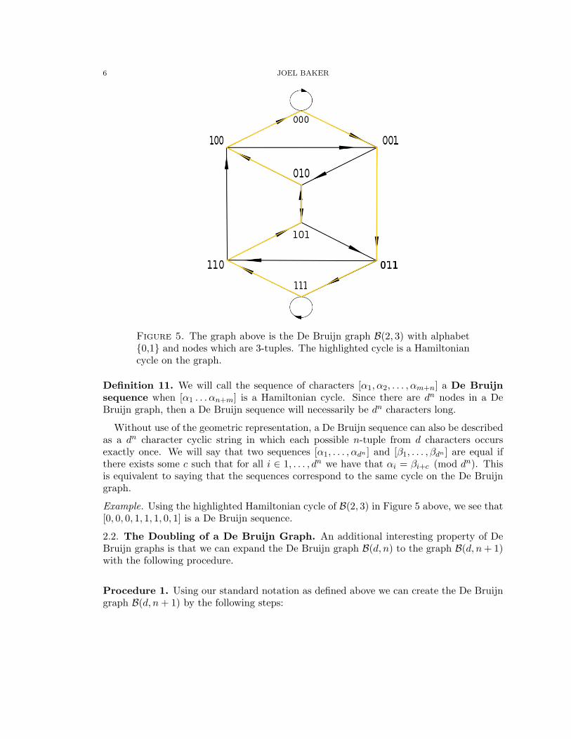
Example. The highlighted cycle in Figure 5 is the Hamiltonian cycle [11010001] which isdescribed by starting at the node (110). We also see that [1111000010011010] is an Euleriancycle on B(2, 3), starting at the node (111).

6 JOEL BAKER

Figure 5. The graph above is the De Bruijn graph B(2, 3) with alphabet{0,1} and nodes which are 3-tuples. The highlighted cycle is a Hamiltoniancycle on the graph.

Definition 11. We will call the sequence of characters [α1, α2, . . . , αm+n] a De Bruijnsequence when [α1 . . . αn+m] is a Hamiltonian cycle. Since there are dn nodes in a DeBruijn graph, then a De Bruijn sequence will necessarily be dn characters long.

Without use of the geometric representation, a De Bruijn sequence can also be describedas a dn character cyclic string in which each possible n-tuple from d characters occursexactly once. We will say that two sequences [α1, . . . , αdn ] and [β1, . . . , βdn ] are equal ifthere exists some c such that for all i ∈ 1, . . . , dn we have that αi = βi+c (mod dn). Thisis equivalent to saying that the sequences correspond to the same cycle on the De Bruijngraph.

Example. Using the highlighted Hamiltonian cycle of B(2, 3) in Figure 5 above, we see that[0, 0, 0, 1, 1, 1, 0, 1] is a De Bruijn sequence.

2.2. The Doubling of a De Bruijn Graph. An additional interesting property of DeBruijn graphs is that we can expand the De Bruijn graph B(d, n) to the graph B(d, n+ 1)with the following procedure.

Procedure 1. Using our standard notation as defined above we can create the De Bruijngraph B(d, n+ 1) by the following steps:

DE BRUIJN GRAPHS AND THEIR APPLICATIONS TO FAULT TOLERANT NETWORKS 7

(1) Construct nodes in B(d, n + 1) from B(d, n) by allowing the edges of B(d, n) tocorrespond to nodes of B(d, n+ 1). Specifically, the adjacent nodes (α1 . . . αn) and(α2 · · ·αn+1) form the edge (α1 . . . αn) (α2 · · ·αn+1) in B(d, n) and correspond tonode (α1 · · ·αn+1) in B(d, n+ 1).

Example. In the doubling from B(3, 3) to B(3, 4) the edge (201)(011) in B(3, 3)gives the node (2011) in B(3, 4)

(2) Construct one edge in B(d, n + 1) for each pair of adjacent edges in B(d, n). Herewe will say that edges are adjacent if the ending node of one edge is the start nodeof the next edge.

The node (α1 . . . αn+1) in B(d, n+1) corresponds to the edge (α1 . . . αn)(α2 . . . αn+1)in B(d, n); the edges leaving (α1 . . . αn+1) are of the form (α1 . . . αn+1)(α2 . . . αn+2).These d edges correspond to the d adjacent edges (α1 . . . αn)(α2 . . . αn+1) and(α2 . . . αn+1)(α3 . . . αn+2) in B(d, n+ 1).

Example. In the doubling from B(3, 3) to B(3, 4) the edge (1222)(2220) in B(3, 4)came from the adjacent edges (122)(222) and (222)(220) in B(3, 3).

See Figure 6 to see an example of the doubling process from B(2, 2) to B(2, 3).

Remark. By Definition 4 and Procedure 1, the number of nodes in B(d, n + 1) (and thusthe number of edges in B(d, n)) ought to be dn+1. The number of edges in B(d, n) is thenumber of nodes, dn, multiplied by the out-degree, d, resulting in dn+1 nodes in B(d, n+1)as desired. Similarly, the number of pairs of adjacent edges in B(d, n) is the product ofthe number of nodes, the in-degree and the out-degree giving dn · d · d = dn+2 which is thenumber of edges that are in B(d, n+ 1).

Figure 6. The graph B(2, 2) (left) getting doubled with intermediate step(middle) to B(2, 3) (right).

8 JOEL BAKER

3. A Combinatorial Problem

De Bruijn’s original paper [dB46] arose from the investigation of a problem concerningthe number of unique De Bruijn sequences with respect to n on the De Bruijn graphB(2, n). De Bruijn was presented [dB46] with the conjecture (see Theorem 1 below) and inhis paper he proves the conjecture using an inductive argument on a type of graph whichis a more general version of the De Bruijn graph.

Theorem 1. The number of De Bruijn sequences contained in B(2, n) is 22n−1−n for alln ≥ 1.

Our goal in this section is to prove the number of De Bruijn sequences contained inB(2, n) is 22n−1−n. However, we must first establish a few important facts.

Definition 12. A T-net of order m is a graph with m nodes and 2m directed edgeswith the property that both the in-degree and out-degree of each node is 2.

For example, notice that B(2, n) is a T-net of order 2n since it has 2n nodes and 2n+1

edges. Let N be a T-net and denote the number of Eulerian cycles of N by |N | (If theT-net is not connected then |N | = 0). We can now construct a unique doubled T-net byusing Procedure 1. This process creates a T-net N∗ of order 2m.

Theorem 2. If N is a T-net of order m and N∗ is its doubled T-net, then

|N∗| = 2m−1|N |.

Proof. We first consider two important cases:

Case 1: N is disconnected.If N is not connected then there will be two nodes with no path between them. If there

was a path in N∗ between every two nodes, then this would imply that there is a path inN from every edge (these correspond to a node in N∗) to every other edge. Thus usingthis ”edge path” we could construct a path of nodes between every pair of nodes in N .Therefore if N∗ is connected then N is connected and so the contrapositive is true as well.Thus, if N is disconnected, N∗ is disconnected. This implies that if N is disconnected,then |N | = |N∗| = 0 and Theorem 2 holds in this case.

Case 2: N is connected and each node has a loop edge.There is only one such connected T-net for each m since after the m loop edges are

counted, the only way to ensure connectivity is to have the remaining edges form a cycleover all m nodes.

Looking at Figure 7 and observing that for any m we will be looking at a regular m-gonwith loops at every edge, we see that for each such T-net, a path that visits each edge willnever have a choice in which edge is taken, thus |N | = 1 in this case.

Next, we will show that |N∗| = 2m−1. For m > 1 we see that since N has m edgeswhich are self loops, then there will be m nodes in N∗ which have self loops. This is adirect result from the doubling procedure. We also see that there will be m nodes in N∗

DE BRUIJN GRAPHS AND THEIR APPLICATIONS TO FAULT TOLERANT NETWORKS 9

Figure 7. This illustrates Case 2 for m = 1, 2, 3 and 4

Figure 8. The corresponding N∗ graphs for m = 1, m = 2 and m = 3.

which do not have self loops, these will correspond to the edges in N which are not selflooping edges. We see they will not have these self loops since these edges are not adjacentto themselves since they have different start and end nodes. We observe that any Eulariancycle on N∗ will only vary on their choice of edge at the m nodes which do not have selfloops. Since each of these m nodes has degree 2 then there will be 2m Eularian cycles, onefor each set of edge choice at the m nodes. However we have double counted these cyclessince any two cycles which take the opposite edge at these m nodes is really the same cyclewritten in a different order. Thus there are 2m−1 Eularian cycles on N∗. Figure 8 showsthis case for the first few m’s.

Thus Theorem 2 holds in this case as well.We now proceed by inducting on the order of the T-net, m. When m = 1 notice that

N is a connected graph and each node has a loop edge, thus it falls into the second caseabove, so Theorem 2 holds when m = 1. We make note that since m = 1, we have that|N | = |N∗|.

10 JOEL BAKER

Now assume inductively that for any T-net, N , of order 1 to m− 1 for m− 1 ≥ 1 that|N∗| = 2m−1|N |.

Consider a T-net, N , of order m. If N is disconnected or if each node has a loop edge,then we are done. If we are not in either of these two cases, we know that there is some nodewhich does not have a loop edge. Call this node α. Since N has in-degree and out-degree2, let the two edges which end at α be called ie1 and ie2 and let the two edges which startat α be called oe1 and oe2. We will also refer to the associated predecessors and successorsof α by A,B,C and D as in Figure 9.

Figure 9. The graph of the node α before removal.

We now create a new graph N1 from N by removing the node α and all of the edges toand from it, but add an edge from C to A and another from D to B as in Figure 10.

Similarly, construct N2 by removing the node α and all of the edges to and from it, butadd an edge from C to B and another from D to A, also in Figure 10.

Figure 10. The partial graphs of N , N1 and N2.

Since our goal is to count Eulerian cycles on the graph, we should note that any Euleriancycle on our T-net N corresponds to an Eulerian cycle on N1 or on N2, but not both. This

DE BRUIJN GRAPHS AND THEIR APPLICATIONS TO FAULT TOLERANT NETWORKS 11

gives us that

(1) |N | = |N1|+ |N2|.

Using Procedure 1 we double the graphs N1 and N2 to create N∗1 and N∗2 respectively.Recall our goal is to show that |N∗| = 2m−1|N |. We have by induction that,

2m−1|N | = 2m−1(|N1|+ |N2|)= 2 · 2m−2|N1|+ 2 · 2m−2|N2|= 2|N∗1 |+ 2|N∗2 |

since both N1 and N2 have m− 1 nodes.All that remains is to show that,

(2) |N∗| = 2|N∗1 |+ 2|N∗2 |.

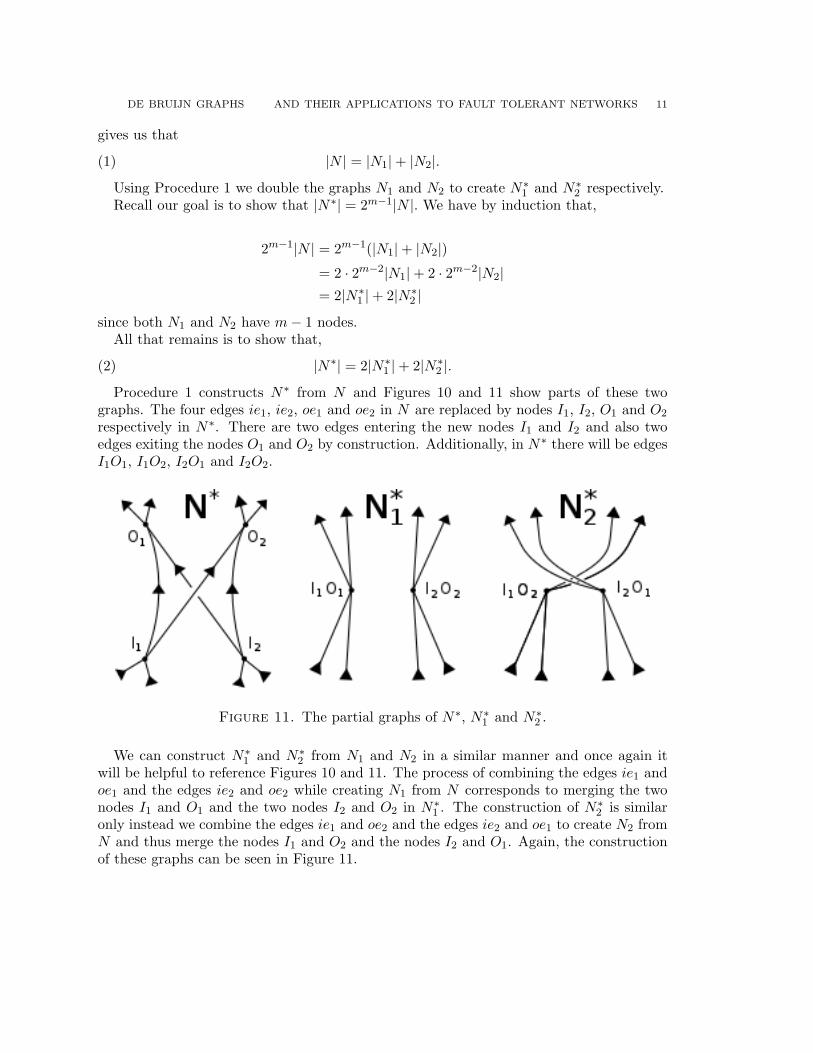
Procedure 1 constructs N∗ from N and Figures 10 and 11 show parts of these twographs. The four edges ie1, ie2, oe1 and oe2 in N are replaced by nodes I1, I2, O1 and O2

respectively in N∗. There are two edges entering the new nodes I1 and I2 and also twoedges exiting the nodes O1 and O2 by construction. Additionally, in N∗ there will be edgesI1O1, I1O2, I2O1 and I2O2.

Figure 11. The partial graphs of N∗, N∗1 and N∗2 .

We can construct N∗1 and N∗2 from N1 and N2 in a similar manner and once again itwill be helpful to reference Figures 10 and 11. The process of combining the edges ie1 andoe1 and the edges ie2 and oe2 while creating N1 from N corresponds to merging the twonodes I1 and O1 and the two nodes I2 and O2 in N∗1 . The construction of N∗2 is similaronly instead we combine the edges ie1 and oe2 and the edges ie2 and oe1 to create N2 fromN and thus merge the nodes I1 and O2 and the nodes I2 and O1. Again, the constructionof these graphs can be seen in Figure 11.

12 JOEL BAKER

Notice now that an Eulerian cycle on N∗ is defined by four paths which have no commonedges, each of which begins at either O1 or O2 and ends at I1 or I2. These paths are edgedisjoint because an Eulerian cycle visits each edge exactly once and these paths are all partof the same Eularian cycle on N . We are assured that each edge except the four edgesI1O1, I1O2, I2O1 and I2O2 will be included in exactly one of these paths since an Euleriancycle traverses every edge. We will be counting the number of Eulerian cycles on N∗, N∗1and N∗2 which contain all four of those paths but differ in their choice of connections of thenodes I1, I2, O1 and O2.

We will adopt N.G. de Bruijn’s notation and construct three more graphs N∗∗, N∗∗1 andN∗∗2 which represent these four paths (discussed above) by single edges instead. Noticethat these new graphs are not the doubled versions of N∗, N∗1 and N∗2 . The additionalgraphs here will help count the number Eularian cycles in N∗ as we proceed by induction.Also, we will now denote |N∗|, |N∗1 |, and |N∗2 | as n, n1 and n2.

In order to show (2) with the new notation, we need to show

(3) n = 2n1 + 2n2.

We consider the following cases:(1) Both paths in N∗ starting from O1 end at different nodes.

Figure 12. Case 1 (left) and Case 2 (right)

As is indicated by the Figure 12 we see that the four paths are: the path fromO1 to I1, from O1 to I2, from O2 to I1 and from O2 to I2.

Upon observing the graph N∗∗ in Figure 12 we see that there are four Euleriancycles. Examining N∗∗1 and N∗∗2 in Figure 13, which are the same graph, we seethat there is exactly one Eulerian cycle. Thus, in this case we establish our claim,since

n = 4 = 2 · 1 + 2 · 1 = 2n1 + 2n2.

DE BRUIJN GRAPHS AND THEIR APPLICATIONS TO FAULT TOLERANT NETWORKS 13

Figure 13. Case 1: N∗∗1 (left) and N∗∗2 (right)

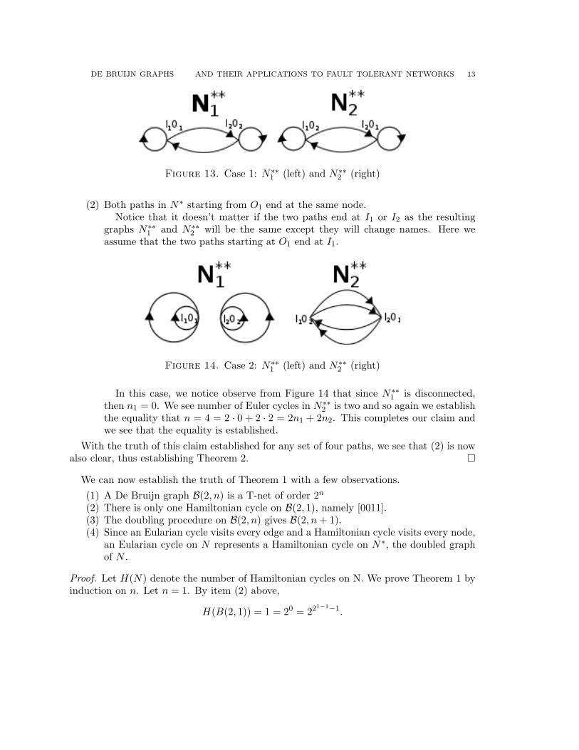
(2) Both paths in N∗ starting from O1 end at the same node.Notice that it doesn’t matter if the two paths end at I1 or I2 as the resulting

graphs N∗∗1 and N∗∗2 will be the same except they will change names. Here weassume that the two paths starting at O1 end at I1.

Figure 14. Case 2: N∗∗1 (left) and N∗∗2 (right)

In this case, we notice observe from Figure 14 that since N∗∗1 is disconnected,then n1 = 0. We see number of Euler cycles in N∗∗2 is two and so again we establishthe equality that n = 4 = 2 · 0 + 2 · 2 = 2n1 + 2n2. This completes our claim andwe see that the equality is established.

With the truth of this claim established for any set of four paths, we see that (2) is nowalso clear, thus establishing Theorem 2. �

We can now establish the truth of Theorem 1 with a few observations.

(1) A De Bruijn graph B(2, n) is a T-net of order 2n

(2) There is only one Hamiltonian cycle on B(2, 1), namely [0011].(3) The doubling procedure on B(2, n) gives B(2, n+ 1).(4) Since an Eularian cycle visits every edge and a Hamiltonian cycle visits every node,

an Eularian cycle on N represents a Hamiltonian cycle on N∗, the doubled graphof N .

Proof. Let H(N) denote the number of Hamiltonian cycles on N. We prove Theorem 1 byinduction on n. Let n = 1. By item (2) above,

H(B(2, 1)) = 1 = 20 = 221−1−1.

14 JOEL BAKER

Now to proceed inductively, let n ≥ 1 and assume that H(B(2, n)) = 22n−1−n. Then,

H(B(2, n+ 1)) =|B(2, n)|=|B(2, n− 1)∗|

=22n−1−1|B(2, n− 1)|

=22n−1−1H(B(2, n))

=22n−1−122n−1−n

=22n−1−1+2n−1−n

=22n−n−1

=22(n+1)−1−(n+1)

Thus our induction holds and the proof of Theorem 1 is complete. �

4. Fault Tolerance

This section is motivated by applications of De Bruijn graphs, and while we will beexamining the mathematical properties relevant to these applications, it is worthwhile tounderstand some motivation. De Bruijn graphs have a few properties which make themnatural choices for the structure of a communication network. Esfahanian and Hakimi[EH85] describe applications of De Bruijn graphs to multiprocessor systems and Collins[CDMP92] describes how the De Bruijn graph gives the structure for a fully parallel Viterbidecoder. De Bruijn graphs have been natural choices for these types of network topologiesfor a few important reasons as follows.

We mentioned in the introduction the first two following properties and now with ourfocus on fault tolerance we find this third property to be valuable as well. For a De Bruijngraph with dn nodes there is a

(1) small in-degree and out-degree, which means fewer connections to each node (pro-cessor)

(2) small distance between nodes (between any two nodes there does not need to existmore than n edges)

(3) large number of paths between nodes.

These properties are the motivation for investigating applications of De Bruijn graphs,and furthermore, since we are interested in the graphs for communication network appli-cations the following questions will be important to study.

(1) What sort of connectivity can we expect to see if a given node is removed?

DE BRUIJN GRAPHS AND THEIR APPLICATIONS TO FAULT TOLERANT NETWORKS 15

(2) What sort of connectivity can we expect to see if an edge is removed?

(3) How many edges can be removed while still maintaining communication paths?

These are the main questions that inspire our mathematical investigation of De Bruijngraphs. As we study the application of De Bruijn graphs we will make these questionsmore precise.

4.1. Node failure. We will first investigate the types of graph structures that result fromnode failures. A node failure is represented by a De Bruijn graph which has that noderemoved as well as all of the edges which begin or end at that particular node.

To investigate these structures, we will prove a few lemmas.

Lemma 1. For any node, α of a De Bruijn graph B(d, n), all of the predecessors of α havethe same set of successors.

Proof. Let α be the node (α1 . . . αn), then any predecessor of α looks like (x α1 · · ·αn−1)for x in our alphabet, and then the successor of any node of this form is (α1 · · ·αn−1 y),with y in our alphabet. �

Example. In B(3, 3) if we look at the node (201) then the set of predecessors will be theset {(020), (120), (220)} and the set of successors for each of those nodes is the same, theyare {(200), (201), (202)}.

Lemma 2. Let α be a node in B(d, n) of the form (α . . . α), then if a node β is neither asuccessor nor a predecessor of α, then α and β have no common successors and they haveno common predecessors (however, a node which is a successor of α could be a predecessorof β and vice versa).

Proof. Any successor of α is of the form (α · · ·α x) where x is a character in our alphabet. Ifα and β share the successor (α · · ·α x) then β is a predecessor of this node. Any predecessorof (α · · ·α x) is of the form (y α · · ·α) for y also a character in our alphabet. Since β is apredecessor of (α · · ·α x), then β = (y α · · ·α) for some choice of y. However, we see byconstruction of B(d, n) that β = (y α · · ·α) is a predecessor of α. Thus if α and β share asuccessor, then β is a predecessor of α.

The proof that if α and β share a predecessor then β is a successor of α is similar. �

Observation 1. Most of the nodes of a De Bruijn graph have disjoint sets of successorsand predecessors. The exception to this is if for a given node (α1 . . . αn) it is the case thatfor some choice of x and y, (x α1α2 · · ·αn−1) = (α2 · · ·αn y). There are three cases wherethis occurs:

(1) When we examine the node (α . . . α).Ex) (111) in B(3, 3) has itself as both a predecessor and a successor.

(2) When n is even, then when we examine the node (αβαβ . . . αβ).Ex) (2020) in B(3, 4) has the node (0202) as both a predecessor and a successor.

16 JOEL BAKER

(3) When n is odd, then when we examine the node (αβαβ . . . α).Ex) (404) in B(5, 3) has the node (040) as both a predecessor and a successor.

Definition 13. Faulty nodes in a graph will be those which are removed from the graph.We will denote the set of faulty nodes in a graph to be the set F . We will refer to the DeBruijn graph B(d, n) with these nodes removed as B(d, n)F .

Remark. When removing F from a De Bruijn graph, we will find that this removal of theindividual nodes might result in a graph on which there exists no Hamiltonian cycles. Wesee that Figure 15 is an example of this since after removing the points (001), (010) and(100) we no longer even have a connected graph.

Figure 15. B(2, 3) (left) with the removal of the points (100), (010) and(001) (right).

It is with this motivation that we introduce this next definition and will later examinea procedure that constructs a cycle on B(d, n)F for a given F , which covers the maximumnumber of nodes.

Definition 14. A necklace of a node, denoted Neck((α1 . . . αn)), is the set of nodes whichare in the cycle [α1 . . . αn+n]

Example. If we examine B(3, 5) then

Neck(21102) = {21102, 11022, 10221, 02211, 22110}.We notice that this is a set of n nodes, but if we examine instead the necklace Neck(2121)in B(3, 4) we see that this set contains only the nodes (2121) and (1212).

Definition 15. The node connectivity of a graph is defined to be the minimum numberof nodes whose removal results in a disconnected graph.

Example. We notice from Figure 15 that the node connectivity of B(2, 3) is at most 3, butupon examination we see that we still have a disconnected graph if only (100) and (001)are removed. This implies that the node connectivity of B(2, 3) is 2 since there is no nodewhose removal results in a disconnected graph.

With the definition of node connectivity and the properties of De Bruijn graphs explored,we are now equipped to answer the question, “What kind of node connectivity can weexpect to see on an undirected De Bruijn graph?”

DE BRUIJN GRAPHS AND THEIR APPLICATIONS TO FAULT TOLERANT NETWORKS 17

Theorem 3 (Thm 2 in [EH85]). The node connectivity of an undirected De Bruijn graph,UB(d, n), is 2d−2. Furthermore, for any arbitrary set of node failures F with |F | ≤ 2d−3,the maximum length of the shortest path between any two nodes is less than or equal to 2n.

A proof of this theorem can be found in [EH85], but we omit it here for brevity, andinstead look at some examples which actualize some of these bounds.

Remark 1. For most nodes of B(d, n) we see that the set of successors and the set ofpredecessors are disjoint (see Observation 1) but when we look at the node (α . . . α) we seethat it has d successors and d predecessors. However, since we are examining the undirectedgraph we see that a node is not considered adjacent to itself, so the node (α . . . α) has 2d−2adjacent nodes. If we remove all of them, then we are clearly left with a disconnected graphas there are no nodes remaining which are adjacent to (α . . . α), thus exhibiting the lowerbound, 2d− 2.

Remark 2. The actualization of the second bound presented on the maximum length ofthe shortest path between nodes is a bit harder construct. The difficulty in construc-tion is explained when Esfahanian and Hakima [EH85] present a slightly better boundof min (2n, n+ 5 + log n) which has an extensive proof that will not be presented in thispaper.

We will now shift our focus back to directed De Bruijn graphs and the approaches takento find bounds on node connectivity.

Lemma 3. Let x be a node in B(2, n), then B(2, n)-Neck(x) has a component with at least2n − n− 1 nodes.

Before beginning the proof of this lemma, it is helpful to examine the following propertiesof necklaces and binary De Bruijn graphs (i.e. those of the form B(2, n)).

Definition 16. Let x be a node in B(2, n), then the weight of x, denoted wt(x), is thenumber of 1’s in x.

With this in mind, we notice the following observations on necklaces and weights.

Observation 2. For every node y ∈ Neck(x) we see that wt(y) = wt(x).

Observation 3. There is only one necklace of weight 0 and n as

Neck(0 . . . 0) = {(0 . . . 0)}and similarly

Neck(1 . . . 1) = {(1 . . . 1)}.

Observation 4. There is only one necklace of weight 1 and n-1 as Neck((1 0 . . . 0)) isthe set of nodes which contain a single 1 and Neck((0 1 . . . 1)) is the set of nodes whichcontain a single 0.

Observation 5. There can be multiple necklaces of weights between 1 and n-1.

Example. In B(2, 4) we see that Neck((1100)) is not the same as Neck((1010))

18 JOEL BAKER

With these facts in mind, we can proceed with the proof of Lemma 3.

Proof. Let x = (x1 . . . xn) be a faulty node in B(2, n) with wt(x) = k. We observe that allof the nodes of weight greater than k are connected since if we have two such nodes y andz with wt(y), wt(z) > k then there is a path from y to z which avoids Neck(x). One suchpath is the path:

(y1 . . . yn)(y2 . . . yn1)(y3 . . . yn11) . . . (1 . . . 1)(1 . . . 1z1)(1 . . . 1z1z2) . . . (1z1 . . . zn−1)(z1 . . . zn).

We see that every node in that path has weight greater than k since the weight is non-decreasing while we add 1’s to the end and then non-increasing when we replace them withthe zi’s until we get to z which has weight greater than k. Similarly, there is a path betweenany two nodes which have weight less than k using the same method with 0’s instead.

We will now prove Lemma 3 in cases on the weight of the faulty node.

• Case wt(x) = 0 (or n): There is only one node of weight 0 and therefore all ofthe nodes have weight greater than this faulty node. We therefore see that B(2, n)- Neck(x) is entirely connected, and thus there is a connected component of size2n − 1.• Case wt(x) = 1 (or n−1): We see that B(2, n) - Neck(x) has no path from (0 · · · 0)

to any other node but that each other node is connected to any other node sinceagain all of the remaining nodes have weight greater than 1. Thus the largestcomponent has size

2n − |Neck(10 . . . 0)| − 1 = 2n − n− 1

• Case 1 < wt(x) < n − 1: We see that this case only arrises when n ≥ 4 since forn < 4 each weight is either in case 1 or case 2 above. By construction we can seethere are at least two necklaces of weight k, for example Neck((0 . . . 01 . . . 1)) andNeck((0 . . . 0101 . . . 1)). Now let y with wt(y) = k and y not in Neck(x). Thenthere is a path from any node with weight less than k to y and there is a path fromany node of weight greater than k to y using the same pathing method as above.We see that both these paths avoid Neck(x) since our path from lesser weight hasnon-decreasing weight and once it has reached a node of weight k it will be a nodein Neck(y). Thus B(2, n) - Neck(x) is connected and then,

2n − |Neck(x)| = 2n − n.

This completes our cases and we see that for all x ∈ B(2, n), the largest connectedcomponent of B(2, n) - Neck(x) has at least 2n − n− 1 nodes. �

Theorem 4. The De Bruijn graph B(2, n) with a single node failure has a cycle with atleast 2n − n− 1 nodes.

Remark. Notice that this statement is very similar to Lemma 3 but it says somethingstronger. We claim instead that not only is there a connected component of size 2n−n− 1but that this component actually contains a cycle.

DE BRUIJN GRAPHS AND THEIR APPLICATIONS TO FAULT TOLERANT NETWORKS 19

We will not discuss this proof in detail, but the method is to apply Lemma 3 and thento apply the following algorithm to construct the cycle. The proof of the correctness ofthis algorithm is in [RB93b].

Let x be a faulty node and let F = Neck(x). The following algorithm constructs thelargest cycle in the component of B(2, n)F which contains the node z. This node is aparameter of the algorithm and so it is important that we choose z to be in the largestcomponent before starting the algorithm. This can be done by choosing wt(z) 6= 0, n.

Algorithm 1 Constructs a Hamiltonian cycle in the component of B(2, n)F which containsthe node zCz := (z)mark zx := zwhile there is an edge from x to an unmarked successor y do

insert y after x in Czmark yx := y

end whilefor each node x in Cz with an unmarked successor y doCy := Cycle(y)Cz := Cz JOIN Cy

end forreturn Cz

Example. In order to understand this algorithm a little better, we will go through anexample of it running on B(2, 4) with faulty node (1100). First, we will remove the necklaceof the faulty node (1100). This set is

F = Neck((1100)) = {(1100), (1001), (0011), (0110)}.

We know from the proof of Lemma 3 that for this particular F , B(2, 4)F is connected andso we can choose any node z at which to start the algorithm.

We start at the node z = (1101), and then build Cz by successively appending nodes tothe end of Cz always choosing from among the successors the first node lexicographicallywhich is unmarked and also not in F . We will continue in this manner until we are at apoint in which there is no successor which is both unmarked and not in F .

The successors of (1101) are (1010) and (1011). At this point only (1101) is marked andneither of these successors are in F , thus our first step will be to add the node (1010) toCz as it is the first, lexicographically, among the successors of (1101). We notice here thatat this point, choosing the successor will generally mean choosing the node which adds a0 to the end because of the lexicographical ordering. This gives,

Cz = (1101)(1010).

20 JOEL BAKER

After this we continue adding nodes to Cz in this fashion so that we obtain

Cz = (1101)(1010)(0100)

= (1101)(1010)(0100)(1000)

= (1101)(1010)(0100)(1000)(0000).

We notice here that the successors of (0000) are (0000) and (0001). The node (0000) hasalready been added to Cz and so it is considered marked and we must instead choose toadd the node (0001). This gives us

Cz = (1101)(1010)(0100)(1000)(0000)(0001)

and then we continue adding nodes again to obtain

Cz = (1101)(1010)(0100)(1000)(0000)(0001)(0010)

= (1101)(1010)(0100)(1000)(0000)(0001)(0010)(0101)

= (1101)(1010)(0100)(1000)(0000)(0001)(0010)(0101)(1011).

It is at this point that since the successors of (1011) are (0110) and (0111), we choose toadd (0111) since (0110) is in the removed set F . We now have

Cz = (1101)(1010)(0100)(1000)(0000)(0001)(0010)(0101)(1011)(0111).

Continuing this process, we add (1110) and then see that with the addition of (1110) thatof the two successors, (1101) is marked and (1100) is in F . Thus we reach the end of the“while” loop with

Cz = (1101)(1010)(0100)(1000)(0000)(0001)(0010)(0101)(1011)(0111)(1110).

We now enter into the “for” loop and try to find the first node which has an unmarkedsuccessor not in F . The first few nodes do not have this property, but we find that thenode (0111) has successor (1111) which is unmarked and not in F .

We now use Algorithm 1 on the node (1111) to construct Cy. We will set y = (1111)and then construct Cy while maintaining the same list of marked nodes as before. Sincethe successors of (1111) are (1111) which is now marked and (1110) which is also markedwe see that Cy = (1111) after the “while loop” completes. Now, after completing theconstruction of Cy, we then go back to our Cz and join it with Cy by inserting Cy after(0111) in Cz. This gives us the cycle

Cz = (1101)(1010)(0100)(1000)(0000)(0001)(0010)(0101)(1011)(0111)(1111)(1110).

This Cz is a cycle on the 12 remaining nodes in B(2, 4) and is therefore a Hamiltonian cycleon the component containing z = (1101).

DE BRUIJN GRAPHS AND THEIR APPLICATIONS TO FAULT TOLERANT NETWORKS 21

Remark. It may appear to be coincidence that this algorithm returns a cycle instead of apath, but if we recall that each predecessor of a node has all same successors, then sinceeach of the predecessors of our start node have been visited, then so, too, must all thesuccessors of those predecessors. This means that since the first node in Cz is the only onewhich has not had an in-going edge and the last node is the only one without an out-goingedge, then this last node must be a predecessor of the original node.

4.2. Edge Failure. We will now turn our attention away from node failure to the topicof edge failure. Notice that it is possible to remove an edge from a De Bruijn graph andstill have a connected graph (for example remove one of the loop edges) so we will beexpecting the bounds on edge failure to be better in the sense that we can remove moreedges and still have connectedness and the existence of Hamiltonian cycles. In this section,we will explore edge failure and the connectivity that we can expect under these failures(i.e. questions 2 and 3 from the beginning of the Fault Tolerance section).

In order to clarify the expression of cycles in this section it will be useful to modify ournotation; from here on the cycle C = [α0 . . . αk−1] will be expressed as

C = [α0, α1, . . . , αk−1]

using commas instead of juxtaposition. Also, our subscripts will be considered modulo kwhere k is the length of the cycle. We will choose d, the size of our alphabet, to either bea prime, or a prime power and thus our alphabet will now be Fd and so we have that thecharacters of the alphabet are the elements of a field. This will allow us to perform somecalculations on nodes and cycles which will be very useful in proving some of the theoremsin this section.

One of the first calculations we will be doing is a character permutation of a cycle. IfC = [c0, c1, . . . , ck−1], then we will say

Cα = [c0 + α, c1 + α, . . . , ck+1 + α].

Additionally, we will adopt the notation of Rowley and Bose [RB93b] and define the cycle

ψ(C) = [c0 − c1, c1 − c2, . . . , ck−1 − c0].

Definition 17. Two cycles are edge disjoint if the set of edges traversed by the firstcycle is disjoint from the set of edges traversed by the second.

Definition 18. A cycle C is edge primitive if the cycles {Cα| 0 ≤ α ≤ d−1} are pairwiseedge disjoint.

Lemma 4. A cycle C in B(d, n) is edge primitive if and only if ψ(C) is a cycle in B(d, n)with no repeated nodes.

Proof. We will just prove the first direction (⇒) here. The proof of the opposite directionuses a similar method (see [RB91]).

Assume C = [c0, c1, . . . , ck−1] is edge primitive. By definition ψ(C) is a cycle and so wewill show that no node can occur twice in ψ(C).

Suppose that

(ci − ci+1, . . . , ci+n−1 − ci+n) = (cj − cj+1, . . . , cj+n−1 − cj+n).

22 JOEL BAKER

We see that if we let δ = cj − ci then,

ci − ci+1 = cj − cj+1 → ci+1 = cj+1 − (cj − ci) = cj+1 − δci+1 − ci+2 = cj+1 − cj+2 → ci+2 = cj+2 − (cj+1 − ci+1) = cj+2 − δ

...ci+n−1 − ci+n = cj+n−1 − cj+n → ci+n = cj+n − δ

This gives us that the cycles C and Cδ have the edge (cici+1 · · · ci+n−1)(ci+1 · · · ci+n) incommon and thus it must be the case that δ = 0. This implies that

ci = cj

ci+1 = cj+1

... =...

ci+n = cj+n

and therefore we see that ψ(C) can have no repeated nodes. �

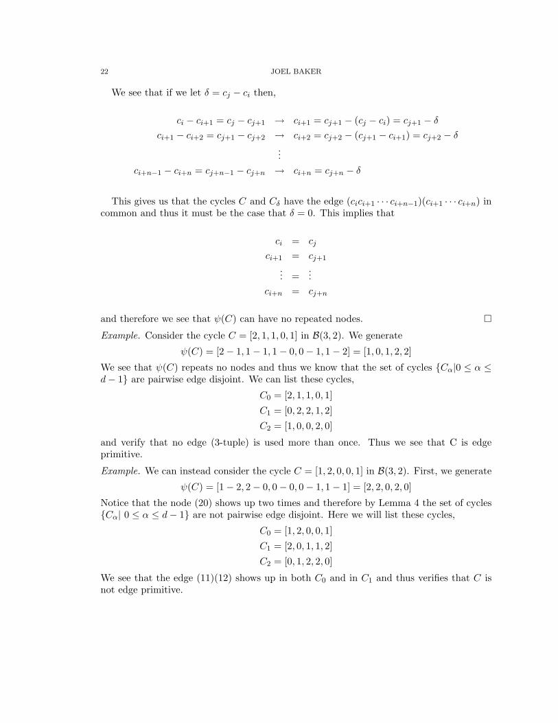
Example. Consider the cycle C = [2, 1, 1, 0, 1] in B(3, 2). We generate

ψ(C) = [2− 1, 1− 1, 1− 0, 0− 1, 1− 2] = [1, 0, 1, 2, 2]

We see that ψ(C) repeats no nodes and thus we know that the set of cycles {Cα|0 ≤ α ≤d− 1} are pairwise edge disjoint. We can list these cycles,

C0 = [2, 1, 1, 0, 1]

C1 = [0, 2, 2, 1, 2]

C2 = [1, 0, 0, 2, 0]

and verify that no edge (3-tuple) is used more than once. Thus we see that C is edgeprimitive.

Example. We can instead consider the cycle C = [1, 2, 0, 0, 1] in B(3, 2). First, we generate

ψ(C) = [1− 2, 2− 0, 0− 0, 0− 1, 1− 1] = [2, 2, 0, 2, 0]

Notice that the node (20) shows up two times and therefore by Lemma 4 the set of cycles{Cα| 0 ≤ α ≤ d− 1} are not pairwise edge disjoint. Here we will list these cycles,

C0 = [1, 2, 0, 0, 1]

C1 = [2, 0, 1, 1, 2]

C2 = [0, 1, 2, 2, 0]

We see that the edge (11)(12) shows up in both C0 and in C1 and thus verifies that C isnot edge primitive.

DE BRUIJN GRAPHS AND THEIR APPLICATIONS TO FAULT TOLERANT NETWORKS 23

The next lemma comes from examining the relationship between cycles in B(d, n) andlinear recurrence relations over Fd.

If we have a sequence S defined by the recurrence relation,

(4) sn+i = an−1sn−1+i + · · ·+ aosi for i ≥ 0

with ai ∈ Fd and a0 6= 0, then the period of S is the smallest k > 0 such that si = si+kfor i ≥ 0. We see then that a sequence with period k corresponds to a cycle of length k inthe De Bruijn graph B(d, n), specifically the cycle [s0, s1, . . . , sk−1].

We will call the polynomial

(5) p(x) = xn − an−1xn−1 − · · · − a1x− a0

the characteristic polynomial of S.

Definition 19. If p(x) is a polynomial over Fd then the order of p(x) is the least positiveinteger k such that p(x) divides 1 − xk. An irreducible polynomial of degree n withcoefficients in Fd is primitive if its order is dn − 1.

Remark. If p(x) is irreducible then from [RB91] the period of S is exactly the order of p(x).From [HP03] we know that there is a primitive polynomial for every choice of n and d (aprime power).

Definition 20. We will say that C = [c0, c1, . . . , ck−1] is a maximal cycle if it is a cyclewith length k = dn−1 and it satisfies a recurrence relation whose characteristic polynomialis primitive.

Lemma 5. If C is a maximal cycle, then C is edge primitive.

Proof. Let C be a maximal cycle which is not edge primitive. Since it is not edge primitive,there exist two cycles, Cα and Cβ which share an edge. This means that the node x =(x0, x1, . . . , xn−1) is followed by the node (x1, . . . , xn−1, xn) in both Cα and Cβ. Then sinceC is generated by the recurrence relation (4) we see that in Cα this implies,

xn = an−1(xn−1 − α) + · · ·+ a0(x0 − α) + α

= an−1xn−1 + · · ·+ a0x0 + (−an−1α− · · · − a0α+ α)d

which implies

xn − an−1xn−1 − · · · − a0x0 = −an−1α− · · · − a0α+ α

= α(1− (an−1 + · · ·+ a0)).

Likewise, in Cβ

xn = an−1(xn−1 − β) + · · ·+ a0(x0 − β) + β

= an−1xn−1 + · · ·+ a0x0 + (−an−1β − · · · − a0β + β).

and so

xn − an−1xn−1 − · · · − a0x0 = −an−1β − · · · − a0β + β

= β(1− (an−1 + · · ·+ a0)).

24 JOEL BAKER

Now from Cα and Cβ we get that

α(1− (an−1 + · · ·+ a0)) = β(1− (an−1 + · · ·+ a0))

and since α 6= β then we see

1− (an−1 + · · ·+ a0) = 0

and then from (5) we see that

p(1) = 1− (an−1 + · · ·+ a0) = 0

and thus (1− x) divides p(x) which contradicts the fact that p(x) is irreducible. Thus Cαand Cβ have no common edges and therefore C is edge primitive.

�

This gives us some cool hardware, so let’s look at an example of this. We would like toconstruct a maximal cycle in B(3, 3). We know that p(x) = x3 + 2x2 + 1 is primitive overFd and so the linear recurrence

xi+3 = −2xi+2 − xi= xi+2 + 2xi(6)

with seeds x0 = x1 = 0 and x2 = 1 should generate our cycle. We continue

x3 =x2 + 2x0

=1 + 2 · 0=1

x4 =x3 + 2x1

=1 + 2 · 0=1

x5 =x4 + 2x2

=1 + 2 · 1=0

. . . = . . .

and so on, continuing to use our recurrence relation to get the next values. This generatesthe cycle

C0 = [00111021121010022201221202].

Then we can construct C1 and C2 by adding 1 and 2 to each value, respectively, giving

C1 =[11222102202121100012002010]

C2 =[22000210010202211120110121].

We see by inspection that C0, C1 and C2 are edge disjoint.

DE BRUIJN GRAPHS AND THEIR APPLICATIONS TO FAULT TOLERANT NETWORKS 25

Theorem 5. The De Bruijn graph B(d, n) with at most d− 1 faulty edges admits a cycleof length dn − 1 when d is a prime power.

Proof. We know that every maximal cycle is a cycle of length dn−1 and also that there ared edge disjoint cycles that we can generate in this manner. This means that these cyclescover

d(dn − 1) = dn+1 − d

edges. We also notice that none of them use the loop edges since then they would visit anode twice.

Additionally, we know from Procedure 1 in Section 2 that there are dn+1 total edges andd loop edges, thus these maximal cycles partition all the dn+1−d edges which are not loopedges. This means that since we have d edge disjoint cycles, that removing d−1 edges fromthe whole graph cannot break all of these cycles and therefore when d is a prime power wesee that B(d, n) still admits at least one of these cycles.

�

Rowley and Bose expand this result to provide a lower bound for De Bruijn graphs whichdo not have alphabets with prime power sizes in [RB93a] . They prove by similar meansin the following Lemmas and Theorem.

Lemma 6. The graph B(d, n) admits d− 1 disjoint Hamiltonian cycles when d is a powerof 2.

Lemma 7. The graph B(d, n) admits d−12 disjoint Hamiltonian cycles when d is an odd

prime power.

We notice that these differ from our previous result in that they are full Hamiltoniancycles and not just cycles of length dn−1 as before. It is this small difference which reducesthe disjoint cycle count.

Lemma 8. If B(d, n) admits k disjoint Hamiltonian cycles, B(d′, n) admits k′ Hamiltoniancycles and d and d′ are relatively prime, then B(dd′, n) admits at least kk′ Hamiltoniancycles.

Theorem 6. The number of disjoint Hamiltonian cycles in B(d, n) is at least

2−kk∏i=1

(piei − 1)

where pe11 · · · pekk is the prime factorization of d.

Proof. The proof of this theorem follows directly from Lemmas 6, 7 and 8.�

26 JOEL BAKER

5. De Bruijn Modifications

We have now seen a variety of modifications to De Bruijn graphs. One particularlysimple modification described in Section 2 was the undirected version of De Bruijn graphs.In Section 3 we saw a generalized version of De Bruijn graphs called a T-net, and in Section4 we examined modifications which result from removing a set of nodes from B(2, n). Inthis section we will consider a few more variants.

5.1. The Qn Cycle. This modification is understood more naturally through the idea ofDe Bruijn sequences, rather than through De Bruijn graphs. At the end of N.G. de Bruijn’spaper [dB46], he presents a problem analogous to that of counting De Bruijn sequencesas discussed in Section 3. He introduces the following sequence which has some uniqueproperties.

Definition 21. A n-tuple is said to be admissible if no two consecutive digits are thesame. A Qn cycle is a string with alphabet {0,1,2} in which every admissible n-tupleoccurs exactly once in the string.

Example. We see that [0,1,2,0,1,0,2,0,2,1,2,1] is a sequence where each admissible 3-tupleoccurs exactly once and thus it fits the criteria to be a Q3 cycle.

We see that like De Bruijn sequences, Qn cycles require each valid n-tuple to occur.However, unlike the De Bruijn sequences presented in [dB46], these revised sequences havea different validity requirement and they also use the alphabet {0,1,2} instead of {0,1}.These cycles do still have a closed formula; In [dB46], De Bruijn gives that the number ofQn cycles is

3 · 23·2n−2−n−1.

This proof here is analogous to the proof presented in Section 3 of Theorem 1.

5.2. Rowley and Bose Modifications. Rowley and Bose cover two additional types ofgraphs in their study of fault tolerance. The first is discussed in [RB91] and it is createdby removing some of the edges and adding them back in other places in order to allow thegraph to have d Hamiltonian cycles instead of the d−1 in standard De Bruijn graphs. Thesecond graph is discussed in [RB93b], and is an undirected version of the first.

Rowley and Bose give a lengthy description of the procedure for the first modificationin [RB91] that will not be presented here. However we will briefly outline the process. Inthe procedure, every self loop is removed and also exactly one edge in every pair of edgesof the form (abab · · · )(baba · · · ) for a 6= b. Then, in order to preserve the in-degree andout-degree of the nodes, some edges of the form (aa · · · )(bb · · · ) and also (abab · · · )(cc · · · )are added.

The new graph will maintain the in-degree and out-degree of the original De Bruijn graphB(d, n) and more importantly will allow us to construct d Hamiltonian cycles on each graphinstead of merely d− 1. This modification is motivated by the practical application of DeBruijn graphs where self loops would be unimportant but better connectivity is. However,through it we lose some of the algebraic structure that was exhibited in the standard DeBruijn graphs.

DE BRUIJN GRAPHS AND THEIR APPLICATIONS TO FAULT TOLERANT NETWORKS 27

Figure 16. B(2, 3) (left) and the modification (right).

The algebraic structure we exhibited in Section 4.2 fails because of the modificationsto the choice of successors for a node. In the original De Bruijn graph we saw that anedge from (α1α2 · · ·αn) to (α2α3 · · ·αn+1) was naturally described using the n + 1 lengthstring α1 · · ·αnαn+1. This property allowed a recurrence relation to choose the next node.However, in this modified graph n+ 1 characters are no longer sufficient to describe everyedge, for example we see this in the case of the edge from (aa · · · a) to (bb · · · b). It is thisproperty that will prohibit our recurrence relations from being able to accurately constructDe Bruijn cycles.

Example. We can look at Figure 16 as an example of this modification on the original DeBruijn graph B(2, 3). The dotted and solid lines each represent edge disjoint Hamiltoniancycles on the graph. We notice here that the modified graph now has 2 such cycles ratherthan the single Hamiltonian cycle that can be constructed on B(2, 3).

The second modification (discussed in [RB93b]) is done with the exact same processexcept to the undirected De Bruijn graph UB(d, n) rather than the directed De Bruijn graphB(d, n). Rowley and Bose discuss how this version of the De Bruijn graph is perhaps astronger model of actual multiprocessor networks since most communication paths betweenprocessors are naturally able to transmit information in both directions.

Example. We can look at Figure 17 below as an example of this modification on theundirected De Bruijn graph UB(2, 3). Again, the dotted and solid lines represent edgedisjoint cycles on the graph.

6. Concluding Statements

In Section 3 we examined N. G. de Bruijn’s original proof in [dB46] that there are 22n−1−n

Hamiltonian cycles in the De Bruijn graph B(2, n). We saw in Section 4.1 that in the case

28 JOEL BAKER

Figure 17. UB(2, 3) (left) and the modification (right).

of a single node failure on B(2, n) that we could use the technique of removing a necklaceto show that these graphs admit cycles of length greater than or equal to 2n − n− 1.

We then saw in Section 4.2 that the standard De Bruijn graph B(d, n) admits at leastone cycle of length dn − 1 under d − 1 edge failures when d is a prime power. In orderto prove this bound we used irreducible polynomials and recurrence relations in order toconstruct these cycles. We then saw from [RB93a] that we could use this knowledge toprovide a lower bound for the number of Hamiltonian cycles on B(d, n) for any d, basedon its prime decomposition.

Lastly, we examined some modifications to De Bruijn graphs and sequences. The Qncycles gave us an example of a different type of structure that we could examine using thetechniques developed in Section 3. Finally, we looked at the modifications presented byRowley and Bose in [RB91] and [RB93b] that yield slightly stronger results but lost someof the original structure.

6.1. Further Directions. There are a few different directions that one could take forfurther research on De Bruijn graphs and their applications. First, we note that the methoddiscussed in Section 4.2 for finding edge disjoint Hamiltonian cycles on De Bruijn graphsis dependent on the fact that our alphabet was chosen with d elements, where d is a primeor prime power. If we choose d to be composite then the current bounds have room forimprovement. Z. Kasa proposes in [Kas10] that the number of edge disjoint Hamiltoniancycles is d − 1. This bound differs greatly from the one proposed by Rowley and Bose in[RB93a] discussed in Section 4.2.

Another direction one could take is to expand the study of node failure to De Bruijngraphs other than binary De Bruijn graphs. Our investigation in Section 4.1 made use ofthe concept of weight which is not immediately applicable to De Bruijn graphs, B(d, n),where d > 2.

DE BRUIJN GRAPHS AND THEIR APPLICATIONS TO FAULT TOLERANT NETWORKS 29

Lastly, we see that one could investigate possible uses for De Bruijn graphs outside offault tolerance. We see from the work of Renault, Scarsini and Tomala [RST07] that DeBruijn graphs can be used to understand the Minority Game in the field of game theory.In addition Delvenne and Carli [DC07] use the De Bruijn graph in their approach tothe Average Consensus Problem, a problem involving communication among independentagents. With these varied applications, we see that De Bruijn graphs are versatile anduseful graphs which are worthy of further investigation.

References

[CDMP92] Oliver Collins, Sam Dolinar, Robert McEliece, and Fabrizio Pollara. A vlsi decomposition ofthe De Bruijn graph. J. ACM, 39:931–948, October 1992.

[dB46] N. G. de Bruijn. A combinatorial problem. Nederl. Akad. Wetensch., Proc., 49:758–764 =Indagationes Math. 8, 461–467 (1946), 1946.

[DC07] J.-C. Delvenne and R. Carli. Optimal strategies in the average consensus problem. In Decisionand Control, 2007 46th IEEE Conference on, pages 2498 –2503, dec. 2007.

[EH85] Abdol-Hossein Esfahanian and S. Louis Hakimi. Fault-tolerant routing in De Bruijn communi-cation networks. IEEE Trans. Comput., 34(9):777–788, 1985.

[HP03] W. C. Huffman and V. Pless. Fundamentals of error-correcting codes. Cambridge Univ. Press,2003.

[Kas10] Zoltan Kasa. On arc-disjoint hamiltonian cycles in De Bruijn graphs. CoRR, abs/1003.1520,2010.

[RB91] R. Rowley and B. Bose. Edge-disjoint hamiltonian cycles in De Bruijn networks. In DistributedMemory Computing Conference, 1991. Proceedings., The Sixth, pages 707 –709, apr-1 may 1991.

[RB93a] Robert Rowley and Bella Bose. On the number of arc-disjoint Hamiltonian circuits in the DeBruijn graph. Parallel Process. Lett., 3(4):375–380, 1993.

[RB93b] Robert A. Rowley and Bella Bose. Fault-tolerant ring embedding in De Bruijn networks. Com-puters, IEEE Transactions on, 42(12):1480 –1486, dec 1993.

[Ros] Vladimir Raphael Rosenfeld. Enumerating De Bruijn sequences. In MATCH Communicationsin Mathematical and in Computer Chemistry, page 2002.

[RST07] Jerome Renault, Marco Scarsini, and Tristan Tomala. A minority game with bounded recall.Math. Oper. Res., 32(4):873–889, 2007.