Introduction - Canadian Discovery Ltd. · Quantitative Seismic Interpretation in the Canadian Oil...
5
“Quantitative Seismic Interpretation in the Canadian Oil Sands” Abstract by Laurie Weston Bellman 2011 Applications and Challenges of Rock Physics for Quantitative Geophysical Interpretation Dubai, U.A.E. – January 15 - 18, 2012 Introduction The Athabasca oil sands contain more than a trillion barrels of bitumen within the Cretaceous formations of northeastern Alberta, Canada. A small portion of this vast resource is close enough to the surface (<75m) to mine but the majority of it must be mapped and developed in-situ. With deposits from 30 – 100m thick at depths of only 100 – 450m, wells are cheap and seismic data is expensive – therefore the Canadian oil sands have always been ‘geology-weighted’ when it comes to evaluation. When the cost of a square kilometer of seismic data is the same as the cost of drilling a well, the geologists’ argument for hard data over soft is often convincing. In an environment where the reservoir is so accessible, it has been a struggle to prove the value of seismic investment. However this reservoir is complex. Even wells drilled 400m apart have sometimes been nearly impossible to correlate – and that’s just the lithology. Fluids are even more unpredictable with variable oil/water contacts fixed in their paleo-positions by biodegraded oil and subsequent tectonics, surprising occurrences of water trapped by bitumen above and below, and top gas (sometimes depleted by previous explorers) and fizzy water ‘thief’ zones which can rob the precious energy carried to the reservoir by injected steam. Short of drilling the wells ever closer together, geophysics is the only solution to the necessary increased sampling of the geology required to solve these problems. Seismic reservoir characterization and quantitative interpretation has played a significant role in the gradual and in some cases, reluctant realization that seismic is critical to understanding reservoir architecture, composition and fluid distribution. So far, the preferred method of in-situ bitumen production is the Steam-Assisted-Gravity-Drainage (SAGD) process. Multiple horizontal well pairs are drilled to inject steam into the reservoir and pump out the heated, liquified oil. The objective of every oil sands operator is to minimize the steam-injected to oil-recovered ratio by maximizing the efficiency of the SAGD process. Reservoir heterogeneity has been found to have the potential for the single most significant negative effect on the efficiency of steam chamber development and overall bitumen recovery, directly influencing steam/oil ratios. Detailed knowledge of the reservoir can therefore allow for better prediction and management of the inherent complexity of the McMurray formation. An accurate baseline reservoir characterization is also essential for subsequent time-lapse seismic analysis and comparison for production monitoring. The process described in this presentation integrates all available data to produce a detailed volume of deterministically derived reservoir, non-reservoir and fluid properties. The workflow is illustrated using examples from two projects in different formations within the Athabasca oil sands. Method As the conceptual flow-chart in Figure 1 shows, rock physics attributes are first determined from seismic data, then classified in terms of facies and fluids using the wireline log and core data from wells. The seismic process involves the use of AVO (amplitude vs offset) analysis to separate the compressional (P- wave) and shear (S-wave) components of the seismic data. The resulting components are then used to calculate physical rock properties such as shear rigidity (mu) and incompressibility (lambda) (Goodway et al. 1997). It is common knowledge among oil sands geoscientists that the density log through the
Transcript of Introduction - Canadian Discovery Ltd. · Quantitative Seismic Interpretation in the Canadian Oil...

“Quantitative Seismic Interpretation in the Canadian Oil Sands” Abstract by Laurie Weston Bellman 2011
Applications and Challenges of Rock Physics for Quantitative Geophysical Interpretation Dubai, U.A.E. – January 15 - 18, 2012
Introduction
The Athabasca oil sands contain more than a trillion barrels of bitumen within the Cretaceous
formations of northeastern Alberta, Canada. A small portion of this vast resource is close enough to the
surface (<75m) to mine but the majority of it must be mapped and developed in-situ. With deposits
from 30 – 100m thick at depths of only 100 – 450m, wells are cheap and seismic data is expensive –
therefore the Canadian oil sands have always been ‘geology-weighted’ when it comes to evaluation.
When the cost of a square kilometer of seismic data is the same as the cost of drilling a well, the
geologists’ argument for hard data over soft is often convincing.
In an environment where the reservoir is so accessible, it has been a struggle to prove the value of
seismic investment. However this reservoir is complex. Even wells drilled 400m apart have sometimes
been nearly impossible to correlate – and that’s just the lithology. Fluids are even more unpredictable
with variable oil/water contacts fixed in their paleo-positions by biodegraded oil and subsequent
tectonics, surprising occurrences of water trapped by bitumen above and below, and top gas
(sometimes depleted by previous explorers) and fizzy water ‘thief’ zones which can rob the precious
energy carried to the reservoir by injected steam. Short of drilling the wells ever closer together,
geophysics is the only solution to the necessary increased sampling of the geology required to solve
these problems. Seismic reservoir characterization and quantitative interpretation has played a
significant role in the gradual and in some cases, reluctant realization that seismic is critical to
understanding reservoir architecture, composition and fluid distribution.
So far, the preferred method of in-situ bitumen production is the Steam-Assisted-Gravity-Drainage
(SAGD) process. Multiple horizontal well pairs are drilled to inject steam into the reservoir and pump
out the heated, liquified oil. The objective of every oil sands operator is to minimize the steam-injected
to oil-recovered ratio by maximizing the efficiency of the SAGD process. Reservoir heterogeneity has
been found to have the potential for the single most significant negative effect on the efficiency of
steam chamber development and overall bitumen recovery, directly influencing steam/oil ratios.
Detailed knowledge of the reservoir can therefore allow for better prediction and management of the
inherent complexity of the McMurray formation. An accurate baseline reservoir characterization is also
essential for subsequent time-lapse seismic analysis and comparison for production monitoring.
The process described in this presentation integrates all available data to produce a detailed volume of
deterministically derived reservoir, non-reservoir and fluid properties. The workflow is illustrated using
examples from two projects in different formations within the Athabasca oil sands.
Method
As the conceptual flow-chart in Figure 1 shows, rock physics attributes are first determined from seismic
data, then classified in terms of facies and fluids using the wireline log and core data from wells. The
seismic process involves the use of AVO (amplitude vs offset) analysis to separate the compressional (P-
wave) and shear (S-wave) components of the seismic data. The resulting components are then used to
calculate physical rock properties such as shear rigidity (mu) and incompressibility (lambda) (Goodway
et al. 1997). It is common knowledge among oil sands geoscientists that the density log through the
Quantitative Seismic Interpretation in the Canadian Oil Sands Laurie Weston Bellman
Applications and Challenges of Rock Physics for Quantitative Geophysical Interpretation Dubai, U.A.E. – January 15 - 18, 2012
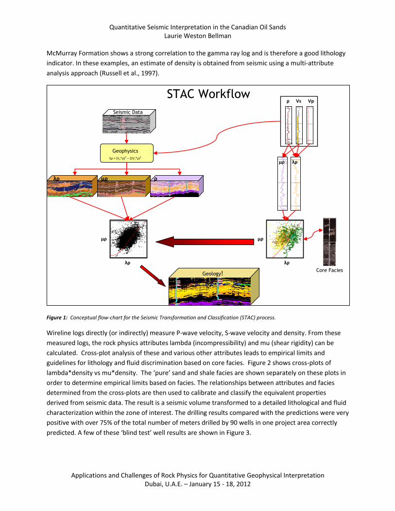
McMurray Formation shows a strong correlation to the gamma ray log and is therefore a good lithology
indicator. In these examples, an estimate of density is obtained from seismic using a multi-attribute
analysis approach (Russell et al., 1997).
Figure 1: Conceptual flow-chart for the Seismic Transformation and Classification (STAC) process.
Wireline logs directly (or indirectly) measure P-wave velocity, S-wave velocity and density. From these
measured logs, the rock physics attributes lambda (incompressibility) and mu (shear rigidity) can be
calculated. Cross-plot analysis of these and various other attributes leads to empirical limits and
guidelines for lithology and fluid discrimination based on core facies. Figure 2 shows cross-plots of
lambda*density vs mu*density. The ‘pure’ sand and shale facies are shown separately on these plots in
order to determine empirical limits based on facies. The relationships between attributes and facies
determined from the cross-plots are then used to calibrate and classify the equivalent properties
derived from seismic data. The result is a seismic volume transformed to a detailed lithological and fluid
characterization within the zone of interest. The drilling results compared with the predictions were very
positive with over 75% of the total number of meters drilled by 90 wells in one project area correctly
predicted. A few of these ‘blind test’ well results are shown in Figure 3.
300
325
350
DEPTHMETRES
LMR.RHO_RP_1K/M31750 2750
LMR.RHO_1K/M31750 2750
dt4pUS/M500 100
298wbsk_c_g_tp
299
mcmr_ch_tp300
top_g_bs5
305top_wat_tp
2307
top_wat_bs3
310
max_pay_tp42
353
max_pay_bs3
355
TOPS.TOPS
WIRE.GR_1GAPI0 200
300
325
350
DEPTHMETRES
LMR.LAMBDA_RHO_1GPA-K/M38000 25000
LMR.MU_RHO_1GPA1000 10000
300
325
350
DEPTHMETRES
WIRE.DT_1US/M500 100
298wbsk_c_g_tp
299
mcmr_ch_tp300
top_g_bs5
305top_wat_tp
2307
top_wat_bs3
310
max_pay_tp42
353
max_pay_bs3
355
TOPS.TOPS
WIRE.GR_1GAPI0 200
300
325
350
DEPTHMETRES
LMR.LAMBDA_RHO_1GPA-K/M38000 25000
LMR.MU_RHO_1GPA1000 10000
ρ Vs Vp
Geophysics
λρ μρ ρ
STAC Workflow
Seismic Data
λρ = (Vp*ρ)2 – 2(Vs*ρ)2 300
325
350
DEPTHMETRES
LMR.RHO_RP_1K/M31750 2750
LMR.RHO_1K/M31750 2750
dt4pUS/M500 100
298wbsk_c_g_tp
299
mcmr_ch_tp300
top_g_bs5
305top_wat_tp
2307
top_wat_bs3
310
max_pay_tp42
353
max_pay_bs3
355
TOPS.TOPS
WIRE.GR_1GAPI0 200
300
325
350
DEPTHMETRES
LMR.LAMBDA_RHO_1GPA-K/M38000 25000
LMR.MU_RHO_1GPA1000 10000
300
325
350
DEPTHMETRES
LMR.RHO_RP_1K/M31750 2750
LMR.RHO_1K/M31750 2750
dt4pUS/M500 100
298wbsk_c_g_tp
299
mcmr_ch_tp300
top_g_bs5
305top_wat_tp
2307
top_wat_bs3
310
max_pay_tp42
353
max_pay_bs3
355
TOPS.TOPS
WIRE.GR_1GAPI0 200
300
325
350
DEPTHMETRES
LMR.LAMBDA_RHO_1GPA-K/M38000 25000
LMR.MU_RHO_1GPA1000 10000
λρ μρ
Filter: FAC_LMR<7&FAC_LMR<>4&SHEAR_QUAL>0.6&BB_FLAG==1Range: All of Well
Well: 47 Wells
LMR.MU_RHO_1 vs. LMR.LAMBDA_RHO_1 Crossplot
0.1 13.4
Color: Maximum of FAC_LMR
Wells:102062507708W400 102110807707W400 1AA011207708W4001AA012107707W400 1AA020807707W400 1AA023507707W4001AA030207708W400 1AA033407707W400 1AA042107707W4001AA052907707W400 1AA053207707W400 1AA061707707W4001AA062307708W400 1AA063407707W400 1AA070207807W4001AA071807707W400 1AA081507708W400 1AA081707707W4001AA082007707W400 1AA082607707W400 1AA082707707W4001AA082807707W400 1AA082907707W400 1AA083007707W4001AA091807608W400 1AA091807707W400 1AA092007608W4001AA092707608W400 1AA092907608W400 1AA101607608W4001AA101607707W400 1AA102807707W400 1AA103407608W4001AA113507608W400 1AA121707708W400 1AA122007707W4001AA122607708W400 1AA142207707W400 1AA143007707W4001AA151807707W400 1AA152807707W400 1AA152907707W4001AB042107708W400 1AB072207708W400 1AB081407708W4001AB123107707W400 1AB142307708W400
Functions:kinosis_mudcurve_cubic : Regression from curve kinosis_mudcurve
MU = (6657.917 - 1.24686*(x) + 8.84e-05*(x)**2- 1.43184e-09*(x)**3)
10
00
0
11
50
0
13
00
0
14
50
0
16
00
0
17
50
0
19
00
0
20
50
0
22
00
0
23
50
0
25
00
0
2000
2600
3200
3800
4400
5000
5600
6200
6800
7400
8000
LM
R.M
U_R
HO
_1 (
)
LMR.LAMBDA_RHO_1 ()
3716
361429
0
24
63
λρ
μρ
Filter: FAC_LMR<7&SHEAR_QUAL>0.6Range: All of Well
Well: 47 Wells
LMR.MU_RHO_1 vs. LMR.LAMBDA_RHO_1 Crossplot
Wells:102062507708W400 102110807707W400 1AA011207708W4001AA012107707W400 1AA020807707W400 1AA023507707W4001AA030207708W400 1AA033407707W400 1AA042107707W4001AA052907707W400 1AA053207707W400 1AA061707707W4001AA062307708W400 1AA063407707W400 1AA070207807W4001AA071807707W400 1AA081507708W400 1AA081707707W4001AA082007707W400 1AA082607707W400 1AA082707707W4001AA082807707W400 1AA082907707W400 1AA083007707W4001AA091807608W400 1AA091807707W400 1AA092007608W4001AA092707608W400 1AA092907608W400 1AA101607608W4001AA101607707W400 1AA102807707W400 1AA103407608W4001AA113507608W400 1AA121707708W400 1AA122007707W4001AA122607708W400 1AA142207707W400 1AA143007707W4001AA151807707W400 1AA152807707W400 1AA152907707W4001AB042107708W400 1AB072207708W400 1AB081407708W4001AB123107707W400 1AB142307708W400
Functions:kinosis_mudcurve_cubic : Regression from curve kinosis_mudcurve
MU = (6657.917 - 1.24686*(x) + 8.84e-05*(x)**2- 1.43184e-09*(x)**3)
80
00
10
20
0
12
40
0
14
60
0
16
80
0
19
00
0
21
20
0
23
40
0
25
60
0
27
80
0
30
00
0
1000
1900
2800
3700
4600
5500
6400
7300
8200
9100
10000
LM
R.M
U_
RH
O_
1 (
)
LMR.LAMBDA_RHO_1 ()
18317
18039183
0
145
99
μρ
λρ
Core Facies Geology!

Quantitative Seismic Interpretation in the Canadian Oil Sands Laurie Weston Bellman
Applications and Challenges of Rock Physics for Quantitative Geophysical Interpretation Dubai, U.A.E. – January 15 - 18, 2012
Filter: (FAC_LMR==5|FAC_LMR==6|FAC_LMR==9)&QUAL_FLAG==1Range: All of Well
Well: 91 Wells
LMR.MU_RHO_1 vs. LMR.LAMBDA_RHO_1 Crossplot
0.1 13.4
Color: Maximum of FACIES_LMR.FAC_LMR
Wells:100_04-32-085-06W4_0 100_05-13-084-07W4_0100_05-32-085-06W4_0 100_06-32-085-06W4_0100_09-31-085-06W4_0 100_12-16-084-07W4_0100_14-36-084-07W4_0 102_01-06-086-06W4_0102_01-31-085-06W4_0 102_05-32-085-06W4_0111_06-36-085-07W4_0 1AA_01-05-086-06W4_01AA_01-35-084-07W4_0 1AA_02-14-084-07W4_01AA_02-23-084-07W4_0 1AA_02-24-084-07W4_01AA_02-36-084-07W4_0 1AA_03-06-086-06W4_01AA_03-20-084-07W4_0 1AA_04-08-086-06W4_01AA_04-16-084-07W4_0 1AA_04-17-086-06W4_01AA_04-23-084-07W4_0 1AA_04-27-084-07W4_01AA_05-15-084-07W4_0 1AA_05-24-084-07W4_01AA_05-25-085-07W4_0 1AA_05-29-085-06W4_01AA_05-36-085-07W4_0 1AA_06-08-086-06W4_01AA_06-29-084-07W4_0 1AA_06-30-084-06W4_01AA_06-33-084-07W4_0 1AA_07-16-084-07W4_01AA_07-22-084-07W4_0 1AA_07-25-084-07W4_01AA_07-25-085-07W4_0 1AA_07-26-084-07W4_01AA_08-08-086-06W4_0 1AA_08-12-086-07W4_01AA_08-32-084-07W4_0 1AA_08-32-085-06W4_01AA_09-07-086-06W4_0 1AA_09-28-084-07W4_01AA_09-29-085-06W4_0 1AA_10-12-086-07W4_01AA_10-13-084-07W4_0 1AA_10-19-084-07W4_01AA_10-21-084-07W4_0 1AA_10-32-084-07W4_01AA_11-12-086-07W4_0 1AA_11-23-084-07W4_01AA_12-25-084-07W4_0 1AA_12-31-084-06W4_01AA_12-35-084-07W4_0 1AA_13-01-086-07W4_01AA_13-07-086-06W4_0 1AA_13-08-086-06W4_01AA_13-13-084-07W4_0 1AA_13-15-084-07W4_01AA_13-24-084-07W4_0 1AA_13-28-084-07W4_01AA_13-29-085-06W4_0 1AA_13-32-084-07W4_01AA_13-32-085-06W4_0 1AA_14-06-086-06W4_01AA_14-14-084-07W4_0 1AA_14-21-084-07W4_01AA_14-26-084-07W4_0 1AA_14-27-084-07W4_01AA_14-31-085-06W4_0 1AA_15-05-086-06W4_01AA_15-16-084-07W4_0 1AA_15-20-084-07W4_01AA_15-24-084-07W4_0 1AA_15-28-084-07W4_01AA_15-29-084-07W4_0 1AA_16-05-086-06W4_01AA_16-13-086-07W4_0 1AA_16-15-084-07W4_01AA_16-17-086-06W4_0 1AA_16-22-084-07W4_01AA_16-27-084-07W4_0 1AA_16-31-085-06W4_01AA_16-33-084-07W4_0 1AA_16-34-084-07W4_01AB_02-31-085-06W4_0 1AB_07-31-085-06W4_01AB_11-12-086-07W4_0 1AB_15-25-085-07W4_01AB_15-36-085-07W4_0
80
00
80
00
10
20
01
02
00
12
40
01
24
00
14
60
01
46
00
16
80
01
68
00
19
00
01
90
00
21
20
02
12
00
23
40
02
34
00
25
60
02
56
00
27
80
02
78
00
30
00
03
00
00
1000 1000
1900 1900
2800 2800
3700 3700
4600 4600
5500 5500
6400 6400
7300 7300
8200 8200
9100 9100
10000 10000
LM
R.M
U_
RH
O_
1 (
)
LMR.LAMBDA_RHO_1 ()
3716
343518
5
7
264
Lambda*rho Lambda*rho
Mu*r
ho
Filter: (FAC_LMR==5|FAC_LMR==6|FAC_LMR==9)&QUAL_FLAG == 1Range: All of Well
Well: 91 Wells
LMR.MU_RHO_1 vs. LMR.LAMBDA_RHO_1 Crossplot
0.1 13.4
Color: Maximum of FACIES_LMR.FAC_LMR
Wells:100_04-32-085-06W4_0 100_05-13-084-07W4_0100_05-32-085-06W4_0 100_06-32-085-06W4_0100_09-31-085-06W4_0 100_12-16-084-07W4_0100_14-36-084-07W4_0 102_01-06-086-06W4_0102_01-31-085-06W4_0 102_05-32-085-06W4_0111_06-36-085-07W4_0 1AA_01-05-086-06W4_01AA_01-35-084-07W4_0 1AA_02-14-084-07W4_01AA_02-23-084-07W4_0 1AA_02-24-084-07W4_01AA_02-36-084-07W4_0 1AA_03-06-086-06W4_01AA_03-20-084-07W4_0 1AA_04-08-086-06W4_01AA_04-16-084-07W4_0 1AA_04-17-086-06W4_01AA_04-23-084-07W4_0 1AA_04-27-084-07W4_01AA_05-15-084-07W4_0 1AA_05-24-084-07W4_01AA_05-25-085-07W4_0 1AA_05-29-085-06W4_01AA_05-36-085-07W4_0 1AA_06-08-086-06W4_01AA_06-29-084-07W4_0 1AA_06-30-084-06W4_01AA_06-33-084-07W4_0 1AA_07-16-084-07W4_01AA_07-22-084-07W4_0 1AA_07-25-084-07W4_01AA_07-25-085-07W4_0 1AA_07-26-084-07W4_01AA_08-08-086-06W4_0 1AA_08-12-086-07W4_01AA_08-32-084-07W4_0 1AA_08-32-085-06W4_01AA_09-07-086-06W4_0 1AA_09-28-084-07W4_01AA_09-29-085-06W4_0 1AA_10-12-086-07W4_01AA_10-13-084-07W4_0 1AA_10-19-084-07W4_01AA_10-21-084-07W4_0 1AA_10-32-084-07W4_01AA_11-12-086-07W4_0 1AA_11-23-084-07W4_01AA_12-25-084-07W4_0 1AA_12-31-084-06W4_01AA_12-35-084-07W4_0 1AA_13-01-086-07W4_01AA_13-07-086-06W4_0 1AA_13-08-086-06W4_01AA_13-13-084-07W4_0 1AA_13-15-084-07W4_01AA_13-24-084-07W4_0 1AA_13-28-084-07W4_01AA_13-29-085-06W4_0 1AA_13-32-084-07W4_01AA_13-32-085-06W4_0 1AA_14-06-086-06W4_01AA_14-14-084-07W4_0 1AA_14-21-084-07W4_01AA_14-26-084-07W4_0 1AA_14-27-084-07W4_01AA_14-31-085-06W4_0 1AA_15-05-086-06W4_01AA_15-16-084-07W4_0 1AA_15-20-084-07W4_01AA_15-24-084-07W4_0 1AA_15-28-084-07W4_01AA_15-29-084-07W4_0 1AA_16-05-086-06W4_01AA_16-13-086-07W4_0 1AA_16-15-084-07W4_01AA_16-17-086-06W4_0 1AA_16-22-084-07W4_01AA_16-27-084-07W4_0 1AA_16-31-085-06W4_01AA_16-33-084-07W4_0 1AA_16-34-084-07W4_01AB_02-31-085-06W4_0 1AB_07-31-085-06W4_01AB_11-12-086-07W4_0 1AB_15-25-085-07W4_01AB_15-36-085-07W4_0
Functions:kinosis_mudcurve_cubic : Regression from curve kinosis_mudcurve
MU = (6657.917 - 1.24686*(x) + 8.84e-05*(x)**2- 1.43184e-09*(x)**3)
80
00
80
00
10
20
01
02
00
12
40
01
24
00
14
60
01
46
00
16
80
01
68
00
19
00
01
90
00
21
20
02
12
00
23
40
02
34
00
25
60
02
56
00
27
80
02
78
00
30
00
03
00
00
1000 1000
1900 1900
2800 2800
3700 3700
4600 4600
5500 5500
6400 6400
7300 7300
8200 8200
9100 9100
10000 10000
LM
R.M
U_
RH
O_
1 (
)
LMR.LAMBDA_RHO_1 ()
3716
343518
5
7
264
Sand Facies Shale FaciesFilter: FAC_LMR==1&QUAL_FLAG == 1
Range: All of WellWell: 92 Wells
LMR.MU_RHO_1 vs. LMR.LAMBDA_RHO_1 Crossplot
6 10
Color: Maximum of FACIES_LMR.FAC_LMR
Wells:100_04-32-085-06W4_0 100_05-13-084-07W4_0100_05-22-084-07W4_0 100_05-32-085-06W4_0100_06-32-085-06W4_0 100_09-31-085-06W4_0100_12-16-084-07W4_0 100_14-36-084-07W4_0102_01-06-086-06W4_0 102_01-31-085-06W4_0102_05-32-085-06W4_0 111_06-36-085-07W4_01AA_01-05-086-06W4_0 1AA_01-35-084-07W4_01AA_02-14-084-07W4_0 1AA_02-23-084-07W4_01AA_02-24-084-07W4_0 1AA_02-36-084-07W4_01AA_03-06-086-06W4_0 1AA_03-20-084-07W4_01AA_04-08-086-06W4_0 1AA_04-16-084-07W4_01AA_04-17-086-06W4_0 1AA_04-23-084-07W4_01AA_04-27-084-07W4_0 1AA_05-15-084-07W4_01AA_05-24-084-07W4_0 1AA_05-25-085-07W4_01AA_05-29-085-06W4_0 1AA_05-36-085-07W4_01AA_06-08-086-06W4_0 1AA_06-29-084-07W4_01AA_06-30-084-06W4_0 1AA_06-33-084-07W4_01AA_07-16-084-07W4_0 1AA_07-22-084-07W4_01AA_07-25-084-07W4_0 1AA_07-25-085-07W4_01AA_07-26-084-07W4_0 1AA_08-08-086-06W4_01AA_08-12-086-07W4_0 1AA_08-32-084-07W4_01AA_08-32-085-06W4_0 1AA_09-07-086-06W4_01AA_09-28-084-07W4_0 1AA_09-29-085-06W4_01AA_10-12-086-07W4_0 1AA_10-13-084-07W4_01AA_10-19-084-07W4_0 1AA_10-21-084-07W4_01AA_10-32-084-07W4_0 1AA_11-12-086-07W4_01AA_11-23-084-07W4_0 1AA_12-25-084-07W4_01AA_12-31-084-06W4_0 1AA_12-35-084-07W4_01AA_13-01-086-07W4_0 1AA_13-07-086-06W4_01AA_13-08-086-06W4_0 1AA_13-13-084-07W4_01AA_13-15-084-07W4_0 1AA_13-24-084-07W4_01AA_13-28-084-07W4_0 1AA_13-29-085-06W4_01AA_13-32-084-07W4_0 1AA_13-32-085-06W4_01AA_14-06-086-06W4_0 1AA_14-14-084-07W4_01AA_14-21-084-07W4_0 1AA_14-26-084-07W4_01AA_14-27-084-07W4_0 1AA_14-31-085-06W4_01AA_15-05-086-06W4_0 1AA_15-16-084-07W4_01AA_15-20-084-07W4_0 1AA_15-24-084-07W4_01AA_15-28-084-07W4_0 1AA_15-29-084-07W4_01AA_16-05-086-06W4_0 1AA_16-13-086-07W4_01AA_16-15-084-07W4_0 1AA_16-17-086-06W4_01AA_16-22-084-07W4_0 1AA_16-27-084-07W4_01AA_16-31-085-06W4_0 1AA_16-33-084-07W4_01AA_16-34-084-07W4_0 1AB_02-31-085-06W4_01AB_07-31-085-06W4_0 1AB_11-12-086-07W4_01AB_15-25-085-07W4_0 1AB_15-36-085-07W4_0
Functions:kinosis_mudcurve_cubic : Regression from curve kinosis_mudcurve
MU = (6657.917 - 1.24686*(x) + 8.84e-05*(x)**2- 1.43184e-09*(x)**3)
80
00
80
00
10
20
01
02
00
12
40
01
24
00
14
60
01
46
00
16
80
01
68
00
19
00
01
90
00
21
20
02
12
00
23
40
02
34
00
25
60
02
56
00
27
80
02
78
00
30
00
03
00
00
1000 1000
1900 1900
2800 2800
3700 3700
4600 4600
5500 5500
6400 6400
7300 7300
8200 8200
9100 9100
10000 10000L
MR
.MU
_R
HO
_1
()
LMR.LAMBDA_RHO_1 ()
8205
812711
0
66 3
Figure 2: Cross plots of computed well logs from 85 wells with dipole sonic logs, separated by core facies. The curve shows the
empirical limit of shale facies which when plotted on the sand facies plot shows the extent of facies overlap. The number of sand
facies points that plot on the shale side of the line is less than 20% of the total.
W E
8675
84 6959 78
Top McMurray
Base McMurray
Top McMurray
Base McMurray
1-21 13-15 12-14 5-14 11-14 7-14 12-13
Within zone of interest – black: non-reservoir (shale or bottom water), light areas: reservoir
Figure 3: Comparison of conventional seismic profile (bottom) with derived facies profile (top). Black represents non-reservoir
(shale or bottom water), yellow is bitumen reservoir, blue is wet reservoir and green is gas reservoir. Gamma ray logs with 0 to
70 (at baseline) api range are displayed on the profiles. 13-15 was the only well on this profile used in the derivation of facies
shown above, the rest were drilled after the facies volume was completed. The numbers shown below the well bores are the
percentage match on a meter-by-meter basis of the predicted facies from seismic with the actual facies from logs within the
zone of interest.
Quantitative Seismic Interpretation in the Canadian Oil Sands Laurie Weston Bellman
Applications and Challenges of Rock Physics for Quantitative Geophysical Interpretation Dubai, U.A.E. – January 15 - 18, 2012
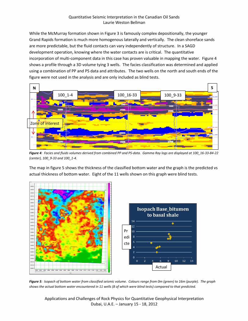
While the McMurray formation shown in Figure 3 is famously complex depositionally, the younger
Grand Rapids formation is much more homogenous laterally and vertically. The clean shoreface sands
are more predictable, but the fluid contacts can vary independently of structure. In a SAGD
development operation, knowing where the water contacts are is critical. The quantitative
incorporation of multi-component data in this case has proven valuable in mapping the water. Figure 4
shows a profile through a 3D volume tying 3 wells. The facies classification was determined and applied
using a combination of PP and PS data and attributes. The two wells on the north and south ends of the
figure were not used in the analysis and are only included as blind tests.
Figure 4: Facies and fluids volumes derived from combined PP and PS-data. Gamma Ray logs are displayed at 100_16-33-84-22
(center), 100_9-33 and 100_1-4.
The map in figure 5 shows the thickness of the classified bottom water and the graph is the predicted vs
actual thickness of bottom water. Eight of the 11 wells shown on this graph were blind tests.
Figure 5: Isopach of bottom water from classified seismic volume. Colours range from 0m (green) to 16m (purple). The graph
shows the actual bottom water encountered in 11 wells (8 of which were blind tests) compared to that predicted.
100_9-33 100_1-4 100_16-33
Zone of interest
N S
Pr
edi
cte
d
Actual

Quantitative Seismic Interpretation in the Canadian Oil Sands Laurie Weston Bellman
Applications and Challenges of Rock Physics for Quantitative Geophysical Interpretation Dubai, U.A.E. – January 15 - 18, 2012
Conclusions
This technique has obvious advantages in an oil sands development project area allowing more
confident identification of the geological features and associated reservoir quality and continuity.
Potential benefits include fewer vertical wells required to define the resource area, more effectively
placed horizontal wells for optimal production and improved steam/oil ratios, as well as flow simulations
based on deterministic facies models. Figure 6 shows an example of a geo-cellular grid containing a
small portion of the facies and fluids volume over a single pair of a proposed 6-well-pair pad. With a
reservoir parameter distribution assigned to the facies, this sub-volume is ready for simulation. After
production has commenced, monitoring of steam injection and heated bitumen can be assessed by
repeating the reservoir characterization process with time-lapse seismic data.
Figure 6: Facies and fluids sub-volume assigned to a geo-cellular grid over a single planned horizontal well pair.
Acknowledgements
The author would like to thank Nexen Canada Inc., Opti Canada Inc. and Laricina Energy Ltd. for
permission to show these data and analysis results.
References
Goodway, W., Chen, T., and Downton, J., [1997], Improved AVO fluid detection and lithology discrimination using Lame
petrophysical parameters; “lambda*rho”, “mu*rho” and “lambda/mu fluid stack”, from P and S inversions, 67th
Annual
International Meeting, SEG Expanded Abstracts, p183-186.
Russell, B., Hampson, D., Schuelke, J., and Quirein, J., [1997], Multi-attribute Seismic Analysis, The Leading Edge, October, 1997,
1439