INTRODUCTION AND BASIC CONCEPTS I - kau 1.pdf · INTRODUCTION AND BASIC CONCEPTS ... tory of the...

I N T R O D U C T I O N A N DB A S I C C O N C E P T S

In this introductory chapter, we present the basic concepts commonly

used in the analysis of fluid flow. We start this chapter with a discussion

of the phases of matter and the numerous ways of classification of fluid

flow, such as viscous versus inviscid regions of flow, internal versus external

flow, compressible versus incompressible flow, laminar versus turbulent

flow, natural versus forced flow, and steady versus unsteady flow. We also

discuss the no-slip condition at solid–fluid interfaces and present a brief his-

tory of the development of fluid mechanics.

After presenting the concepts of system and control volume, we review

the unit systems that will be used. We then discuss how mathematical mod-

els for engineering problems are prepared and how to interpret the results

obtained from the analysis of such models. This is followed by a presenta-

tion of an intuitive systematic problem-solving technique that can be used as

a model in solving engineering problems. Finally, we discuss accuracy, pre-

cision, and significant digits in engineering measurements and calculations.

1

CHAPTER

1OBJECTIVES

When you finish reading this chapter, you

should be able to

� Understand the basic concepts

of fluid mechanics and recognize

the various types of fluid flow

problems encountered in

practice

� Model engineering problems and

solve them in a systematic

manner

� Have a working knowledge of

accuracy, precision, and

significant digits, and recognize

the importance of dimensional

homogeneity in engineering

calculations

cen72367_ch01.qxd 10/29/04 2:31 PM

1–1 � INTRODUCTION

Mechanics is the oldest physical science that deals with both stationary andmoving bodies under the influence of forces. The branch of mechanics thatdeals with bodies at rest is called statics, while the branch that deals withbodies in motion is called dynamics. The subcategory fluid mechanics isdefined as the science that deals with the behavior of fluids at rest (fluid sta-

tics) or in motion (fluid dynamics), and the interaction of fluids with solidsor other fluids at the boundaries. Fluid mechanics is also referred to as fluid

dynamics by considering fluids at rest as a special case of motion with zerovelocity (Fig. 1–1).

Fluid mechanics itself is also divided into several categories. The study ofthe motion of fluids that are practically incompressible (such as liquids,especially water, and gases at low speeds) is usually referred to as hydrody-

namics. A subcategory of hydrodynamics is hydraulics, which deals with liq-uid flows in pipes and open channels. Gas dynamics deals with the flow offluids that undergo significant density changes, such as the flow of gasesthrough nozzles at high speeds. The category aerodynamics deals with theflow of gases (especially air) over bodies such as aircraft, rockets, and automo-biles at high or low speeds. Some other specialized categories such as meteo-

rology, oceanography, and hydrology deal with naturally occurring flows.

What Is a Fluid?You will recall from physics that a substance exists in three primary phases:solid, liquid, and gas. (At very high temperatures, it also exists as plasma.)A substance in the liquid or gas phase is referred to as a fluid. Distinctionbetween a solid and a fluid is made on the basis of the substance’s ability toresist an applied shear (or tangential) stress that tends to change its shape. Asolid can resist an applied shear stress by deforming, whereas a fluiddeforms continuously under the influence of shear stress, no matter howsmall. In solids stress is proportional to strain, but in fluids stress is propor-tional to strain rate. When a constant shear force is applied, a solid eventu-ally stops deforming, at some fixed strain angle, whereas a fluid never stopsdeforming and approaches a certain rate of strain.

Consider a rectangular rubber block tightly placed between two plates. Asthe upper plate is pulled with a force F while the lower plate is held fixed,the rubber block deforms, as shown in Fig. 1–2. The angle of deformation a(called the shear strain or angular displacement) increases in proportion tothe applied force F. Assuming there is no slip between the rubber and theplates, the upper surface of the rubber is displaced by an amount equal tothe displacement of the upper plate while the lower surface remains station-ary. In equilibrium, the net force acting on the plate in the horizontal direc-tion must be zero, and thus a force equal and opposite to F must be actingon the plate. This opposing force that develops at the plate–rubber interfacedue to friction is expressed as F � tA, where t is the shear stress and A isthe contact area between the upper plate and the rubber. When the force isremoved, the rubber returns to its original position. This phenomenon wouldalso be observed with other solids such as a steel block provided that theapplied force does not exceed the elastic range. If this experiment wererepeated with a fluid (with two large parallel plates placed in a large bodyof water, for example), the fluid layer in contact with the upper plate would

2FLUID MECHANICS

FIGURE 1–1

Fluid mechanics deals with liquids andgases in motion or at rest.

© Vol. 16/Photo Disc.

Contact area,A

Shear stresst = F/A

Shearstrain, a

Force, F

aDeformed

rubber

FIGURE 1–2

Deformation of a rubber eraser placedbetween two parallel plates under theinfluence of a shear force.

cen72367_ch01.qxd 10/29/04 2:31 PM

move with the plate continuously at the velocity of the plate no matter howsmall the force F is. The fluid velocity decreases with depth because of fric-tion between fluid layers, reaching zero at the lower plate.

You will recall from statics that stress is defined as force per unit areaand is determined by dividing the force by the area upon which it acts. Thenormal component of the force acting on a surface per unit area is called thenormal stress, and the tangential component of a force acting on a surfaceper unit area is called shear stress (Fig. 1–3). In a fluid at rest, the normalstress is called pressure. The supporting walls of a fluid eliminate shearstress, and thus a fluid at rest is at a state of zero shear stress. When thewalls are removed or a liquid container is tilted, a shear develops and theliquid splashes or moves to attain a horizontal free surface.

In a liquid, chunks of molecules can move relative to each other, but thevolume remains relatively constant because of the strong cohesive forcesbetween the molecules. As a result, a liquid takes the shape of the containerit is in, and it forms a free surface in a larger container in a gravitationalfield. A gas, on the other hand, expands until it encounters the walls of thecontainer and fills the entire available space. This is because the gas mole-cules are widely spaced, and the cohesive forces between them are verysmall. Unlike liquids, gases cannot form a free surface (Fig. 1–4).

Although solids and fluids are easily distinguished in most cases, this dis-tinction is not so clear in some borderline cases. For example, asphalt appearsand behaves as a solid since it resists shear stress for short periods of time.But it deforms slowly and behaves like a fluid when these forces are exertedfor extended periods of time. Some plastics, lead, and slurry mixtures exhibitsimilar behavior. Such borderline cases are beyond the scope of this text. Thefluids we will deal with in this text will be clearly recognizable as fluids.

Intermolecular bonds are strongest in solids and weakest in gases. Onereason is that molecules in solids are closely packed together, whereas ingases they are separated by relatively large distances (Fig. 1–5).

The molecules in a solid are arranged in a pattern that is repeated through-out. Because of the small distances between molecules in a solid, the attrac-tive forces of molecules on each other are large and keep the molecules at

3CHAPTER 1

Fn

Ft

F

Normalto surface

Tangentto surface

Force actingon area dA

dA

FIGURE 1–3

The normal stress and shear stress atthe surface of a fluid element. For

fluids at rest, the shear stress is zeroand pressure is the only normal stress.

Free surface

Liquid Gas

FIGURE 1–4

Unlike a liquid, a gas does not form afree surface, and it expands to fill the

entire available space.

(a) (b) (c)

FIGURE 1–5

The arrangement of atoms in different phases: (a) molecules are at relatively fixed positionsin a solid, (b) groups of molecules move about each other in the liquid phase, and

(c) molecules move about at random in the gas phase.

Shear stress: t�Ft

dA

Normal stress: s �Fn

dA

cen72367_ch01.qxd 10/29/04 2:31 PM

fixed positions. The molecular spacing in the liquid phase is not much differ-ent from that of the solid phase, except the molecules are no longer at fixedpositions relative to each other and they can rotate and translate freely. In aliquid, the intermolecular forces are weaker relative to solids, but still strongcompared with gases. The distances between molecules generally increaseslightly as a solid turns liquid, with water being a notable exception.

In the gas phase, the molecules are far apart from each other, and a mole-cular order is nonexistent. Gas molecules move about at random, continu-ally colliding with each other and the walls of the container in which theyare contained. Particularly at low densities, the intermolecular forces arevery small, and collisions are the only mode of interaction between the mol-ecules. Molecules in the gas phase are at a considerably higher energy levelthan they are in the liquid or solid phase. Therefore, the gas must release alarge amount of its energy before it can condense or freeze.

Gas and vapor are often used as synonymous words. The vapor phase of asubstance is customarily called a gas when it is above the critical tempera-ture. Vapor usually implies a gas that is not far from a state of condensation.

Any practical fluid system consists of a large number of molecules, andthe properties of the system naturally depend on the behavior of these mole-cules. For example, the pressure of a gas in a container is the result ofmomentum transfer between the molecules and the walls of the container.However, one does not need to know the behavior of the gas molecules todetermine the pressure in the container. It would be sufficient to attach apressure gage to the container (Fig. 1–6). This macroscopic or classical

approach does not require a knowledge of the behavior of individual mole-cules and provides a direct and easy way to the solution of engineeringproblems. The more elaborate microscopic or statistical approach, based onthe average behavior of large groups of individual molecules, is ratherinvolved and is used in this text only in the supporting role.

Application Areas of Fluid MechanicsFluid mechanics is widely used both in everyday activities and in the designof modern engineering systems from vacuum cleaners to supersonic aircraft.Therefore, it is important to develop a good understanding of the basic prin-ciples of fluid mechanics.

To begin with, fluid mechanics plays a vital role in the human body. Theheart is constantly pumping blood to all parts of the human body throughthe arteries and veins, and the lungs are the sites of airflow in alternatingdirections. Needless to say, all artificial hearts, breathing machines, anddialysis systems are designed using fluid dynamics.

An ordinary house is, in some respects, an exhibition hall filled with appli-cations of fluid mechanics. The piping systems for cold water, natural gas,and sewage for an individual house and the entire city are designed primarilyon the basis of fluid mechanics. The same is also true for the piping and duct-ing network of heating and air-conditioning systems. A refrigerator involvestubes through which the refrigerant flows, a compressor that pressurizes therefrigerant, and two heat exchangers where the refrigerant absorbs and rejectsheat. Fluid mechanics plays a major role in the design of all these compo-nents. Even the operation of ordinary faucets is based on fluid mechanics.

We can also see numerous applications of fluid mechanics in an automo-bile. All components associated with the transportation of the fuel from the

4FLUID MECHANICS

Pressuregage

FIGURE 1–6

On a microscopic scale, pressure isdetermined by the interaction ofindividual gas molecules. However,we can measure the pressure on amacroscopic scale with a pressuregage.

cen72367_ch01.qxd 10/29/04 2:31 PM

fuel tank to the cylinders—the fuel line, fuel pump, fuel injectors, or carbu-retors—as well as the mixing of the fuel and the air in the cylinders and thepurging of combustion gases in exhaust pipes are analyzed using fluidmechanics. Fluid mechanics is also used in the design of the heating andair-conditioning system, the hydraulic brakes, the power steering, automatictransmission, and lubrication systems, the cooling system of the engineblock including the radiator and the water pump, and even the tires. Thesleek streamlined shape of recent model cars is the result of efforts to mini-mize drag by using extensive analysis of flow over surfaces.

On a broader scale, fluid mechanics plays a major part in the design andanalysis of aircraft, boats, submarines, rockets, jet engines, wind turbines,biomedical devices, the cooling of electronic components, and the trans-portation of water, crude oil, and natural gas. It is also considered in thedesign of buildings, bridges, and even billboards to make sure that the struc-tures can withstand wind loading. Numerous natural phenomena such as therain cycle, weather patterns, the rise of ground water to the top of trees,winds, ocean waves, and currents in large water bodies are also governed bythe principles of fluid mechanics (Fig. 1–7).

5CHAPTER 1

Piping and plumbing systems

Photo by John M. Cimbala.

Cars

Photo by John M. Cimbala.

Power plants


Aircraft and spacecraft


Human body


Wind turbines


Natural flows and weather


Industrial applications

Courtesy UMDE Engineering, Contracting,

and Trading. Used by permission.

FIGURE 1–7

Some application areas of fluid mechanics.

Boats


cen72367_ch01.qxd 10/29/04 2:31 PM

1–2 � THE NO-SLIP CONDITION

Fluid flow is often confined by solid surfaces, and it is important to under-stand how the presence of solid surfaces affects fluid flow. We know thatwater in a river cannot flow through large rocks, and goes around them.That is, the water velocity normal to the rock surface must be zero, andwater approaching the surface normally comes to a complete stop at the sur-face. What is not so obvious is that water approaching the rock at any anglealso comes to a complete stop at the rock surface, and thus the tangentialvelocity of water at the surface is also zero.

Consider the flow of a fluid in a stationary pipe or over a solid surfacethat is nonporous (i.e., impermeable to the fluid). All experimental observa-tions indicate that a fluid in motion comes to a complete stop at the surfaceand assumes a zero velocity relative to the surface. That is, a fluid in directcontact with a solid “sticks” to the surface due to viscous effects, and thereis no slip. This is known as the no-slip condition.

The photo in Fig. 1–8 obtained from a video clip clearly shows the evolu-tion of a velocity gradient as a result of the fluid sticking to the surface of ablunt nose. The layer that sticks to the surface slows the adjacent fluid layerbecause of viscous forces between the fluid layers, which slows the nextlayer, and so on. Therefore, the no-slip condition is responsible for thedevelopment of the velocity profile. The flow region adjacent to the wall inwhich the viscous effects (and thus the velocity gradients) are significant iscalled the boundary layer. The fluid property responsible for the no-slipcondition and the development of the boundary layer is viscosity and is dis-cussed in Chap. 2.

A fluid layer adjacent to a moving surface has the same velocity as thesurface. A consequence of the no-slip condition is that all velocity profilesmust have zero values with respect to the surface at the points of contactbetween a fluid and a solid surface (Fig. 1–9). Another consequence of theno-slip condition is the surface drag, which is the force a fluid exerts on asurface in the flow direction.

When a fluid is forced to flow over a curved surface, such as the backside of a cylinder at sufficiently high velocity, the boundary layer can nolonger remain attached to the surface, and at some point it separates fromthe surface—a process called flow separation (Fig. 1–10). We emphasizethat the no-slip condition applies everywhere along the surface, even down-stream of the separation point. Flow separation is discussed in greater detailin Chap. 10.

6FLUID MECHANICS

FIGURE 1–8

The development of a velocity profiledue to the no-slip condition as a fluidflows over a blunt nose.

“Hunter Rouse: Laminar and Turbulent Flow Film.”

Copyright IIHR-Hydroscience & Engineering,

The University of Iowa. Used by permission.

Relativevelocitiesof fluid layers

Uniformapproachvelocity, V

Zero velocityat the surface

Plate

FIGURE 1–9

A fluid flowing over a stationarysurface comes to a complete stop atthe surface because of the no-slipcondition.

Separation point

FIGURE 1–10

Flow separation during flow over a curved surface.

From G. M. Homsy et al, “Multi-Media Fluid Mechanics,” Cambridge Univ.

Press (2001). ISBN 0-521-78748-3. Reprinted by permission.

cen72367_ch01.qxd 10/29/04 2:32 PM

A similar phenomenon occurs for temperature. When two bodies at differ-ent temperatures are brought into contact, heat transfer occurs until bothbodies assume the same temperature at the points of contact. Therefore, afluid and a solid surface have the same temperature at the points of contact.This is known as no-temperature-jump condition.

1–3 � A BRIEF HISTORY OF FLUID MECHANICS1

One of the first engineering problems humankind faced as cities were devel-oped was the supply of water for domestic use and irrigation of crops. Oururban lifestyles can be retained only with abundant water, and it is clearfrom archeology that every successful civilization of prehistory invested inthe construction and maintenance of water systems. The Roman aqueducts,some of which are still in use, are the best known examples. However, per-haps the most impressive engineering from a technical viewpoint was doneat the Hellenistic city of Pergamon in present-day Turkey. There, from 283to 133 BC, they built a series of pressurized lead and clay pipelines (Fig.1–11), up to 45 km long that operated at pressures exceeding 1.7 MPa (180m of head). Unfortunately, the names of almost all these early builders arelost to history. The earliest recognized contribution to fluid mechanics the-ory was made by the Greek mathematician Archimedes (285–212 BC). Heformulated and applied the buoyancy principle in history’s first nondestruc-tive test to determine the gold content of the crown of King Hiero I. TheRomans built great aqueducts and educated many conquered people on thebenefits of clean water, but overall had a poor understanding of fluids the-ory. (Perhaps they shouldn’t have killed Archimedes when they sackedSyracuse.)

During the Middle Ages the application of fluid machinery slowly butsteadily expanded. Elegant piston pumps were developed for dewateringmines, and the watermill and windmill were perfected to grind grain, forgemetal, and for other tasks. For the first time in recorded human history sig-nificant work was being done without the power of a muscle supplied by aperson or animal, and these inventions are generally credited with enablingthe later industrial revolution. Again the creators of most of the progress areunknown, but the devices themselves were well documented by severaltechnical writers such as Georgius Agricola (Fig. 1–12).

The Renaissance brought continued development of fluid systems andmachines, but more importantly, the scientific method was perfected andadopted throughout Europe. Simon Stevin (1548–1617), Galileo Galilei(1564–1642), Edme Mariotte (1620–1684), and Evangelista Torricelli(1608–1647) were among the first to apply the method to fluids as theyinvestigated hydrostatic pressure distributions and vacuums. That work wasintegrated and refined by the brilliant mathematician, Blaise Pascal (1623–1662). The Italian monk, Benedetto Castelli (1577–1644) was the first per-son to publish a statement of the continuity principle for fluids. Besides for-mulating his equations of motion for solids, Sir Isaac Newton (1643–1727)applied his laws to fluids and explored fluid inertia and resistance, free jets,and viscosity. That effort was built upon by the Swiss Daniel Bernoulli

7CHAPTER 1

1 This section is contributed by Professor Glenn Brown of Oklahoma State University.

FIGURE 1–11

Segment of Pergamon pipeline. Each clay pipe section was

13 to 18 cm in diameter.

Courtesy Gunther Garbrecht.

Used by permission.

FIGURE 1–12

A mine hoist powered by a reversible water wheel.

G. Agricola, De Re Metalica, Basel, 1556.

cen72367_ch01.qxd 10/29/04 2:32 PM

(1700–1782) and his associate Leonard Euler (1707–1783). Together, theirwork defined the energy and momentum equations. Bernoulli’s 1738 classictreatise Hydrodynamica may be considered the first fluid mechanics text.Finally, Jean d’Alembert (1717–1789) developed the idea of velocity andacceleration components, a differential expression of continuity, and his“paradox” of zero resistance to steady uniform motion.

The development of fluid mechanics theory up through the end of theeighteenth century had little impact on engineering since fluid propertiesand parameters were poorly quantified, and most theories were abstractionsthat could not be quantified for design purposes. That was to change withthe development of the French school of engineering led by Riche de Prony(1755–1839). Prony (still known for his brake to measure power) and hisassociates in Paris at the Ecole Polytechnic and the Ecole Ponts et Chausseeswere the first to integrate calculus and scientific theory into the engineeringcurriculum, which became the model for the rest of the world. (So nowyou know whom to blame for your painful freshman year.) Antonie Chezy(1718–1798), Louis Navier (1785–1836), Gaspard Coriolis (1792–1843),Henry Darcy (1803–1858), and many other contributors to fluid engineeringand theory were students and/or instructors at the schools.

By the mid nineteenth century fundamental advances were coming onseveral fronts. The physician Jean Poiseuille (1799–1869) had accuratelymeasured flow in capillary tubes for multiple fluids, while in GermanyGotthilf Hagen (1797–1884) had differentiated between laminar and turbu-lent flow in pipes. In England, Lord Osborn Reynolds (1842–1912) contin-ued that work and developed the dimensionless number that bears his name.Similarly, in parallel to the early work of Navier, George Stokes (1819–1903) completed the general equations of fluid motion with friction thattake their names. William Froude (1810–1879) almost single-handedlydeveloped the procedures and proved the value of physical model testing.American expertise had become equal to the Europeans as demonstrated byJames Francis’s (1815–1892) and Lester Pelton’s (1829–1908) pioneeringwork in turbines and Clemens Herschel’s (1842–1930) invention of the Ven-turi meter.

The late nineteenth century was notable for the expansion of fluid theoryby Irish and English scientists and engineers, including in addition toReynolds and Stokes, William Thomson, Lord Kelvin (1824–1907), WilliamStrutt, Lord Rayleigh (1842–1919), and Sir Horace Lamb (1849–1934).These individuals investigated a large number of problems including dimen-sional analysis, irrotational flow, vortex motion, cavitation, and waves. In abroader sense their work also explored the links between fluid mechanics,thermodynamics, and heat transfer.

The dawn of the twentieth century brought two monumental develop-ments. First in 1903, the self-taught Wright brothers (Wilbur, 1867–1912;Orville, 1871–1948) through application of theory and determined experi-mentation perfected the airplane. Their primitive invention was completeand contained all the major aspects of modern craft (Fig. 1–13). TheNavier–Stokes equations were of little use up to this time because they weretoo difficult to solve. In a pioneering paper in 1904, the German LudwigPrandtl (1875–1953) showed that fluid flows can be divided into a layernear the walls, the boundary layer, where the friction effects are significantand an outer layer where such effects are negligible and the simplified Euler

8FLUID MECHANICS

FIGURE 1–13

The Wright brothers take flight at Kitty Hawk.

National Air and Space Museum/

Smithsonian Institution.

cen72367_ch01.qxd 10/29/04 2:32 PM

and Bernoulli equations are applicable. His students, Theodore von Kármán(1881–1963), Paul Blasius (1883–1970), Johann Nikuradse (1894–1979),and others, built on that theory in both hydraulic and aerodynamic applica-tions. (During World War II, both sides benefited from the theory as Prandtlremained in Germany while his best student, the Hungarian born von Kár-mán, worked in America.)

The mid twentieth century could be considered a golden age of fluidmechanics applications. Existing theories were adequate for the tasks athand, and fluid properties and parameters were well defined. These sup-ported a huge expansion of the aeronautical, chemical, industrial, and waterresources sectors; each of which pushed fluid mechanics in new directions.Fluid mechanics research and work in the late twentieth century were domi-nated by the development of the digital computer in America. The ability tosolve large complex problems, such as global climate modeling or to opti-mize the design of a turbine blade, has provided a benefit to our society thatthe eighteenth-century developers of fluid mechanics could never haveimagined (Fig. 1–14). The principles presented in the following pages havebeen applied to flows ranging from a moment at the microscopic scale to 50years of simulation for an entire river basin. It is truly mind-boggling.

Where will fluid mechanics go in the twenty-first century? Frankly, evena limited extrapolation beyond the present would be sheer folly. However, ifhistory tells us anything, it is that engineers will be applying what theyknow to benefit society, researching what they don’t know, and having agreat time in the process.

1–4 � CLASSIFICATION OF FLUID FLOWS

Earlier we defined fluid mechanics as the science that deals with the behav-ior of fluids at rest or in motion, and the interaction of fluids with solids orother fluids at the boundaries. There is a wide variety of fluid flow problemsencountered in practice, and it is usually convenient to classify them on thebasis of some common characteristics to make it feasible to study them ingroups. There are many ways to classify fluid flow problems, and here wepresent some general categories.

Viscous versus Inviscid Regions of FlowWhen two fluid layers move relative to each other, a friction force developsbetween them and the slower layer tries to slow down the faster layer. Thisinternal resistance to flow is quantified by the fluid property viscosity,which is a measure of internal stickiness of the fluid. Viscosity is caused bycohesive forces between the molecules in liquids and by molecular colli-sions in gases. There is no fluid with zero viscosity, and thus all fluid flowsinvolve viscous effects to some degree. Flows in which the frictional effectsare significant are called viscous flows. However, in many flows of practicalinterest, there are regions (typically regions not close to solid surfaces)where viscous forces are negligibly small compared to inertial or pressureforces. Neglecting the viscous terms in such inviscid flow regions greatlysimplifies the analysis without much loss in accuracy.

The development of viscous and inviscid regions of flow as a result ofinserting a flat plate parallel into a fluid stream of uniform velocity isshown in Fig. 1–15. The fluid sticks to the plate on both sides because of

9CHAPTER 1

FIGURE 1–14

The Oklahoma Wind Power Centernear Woodward consists of 68

turbines, 1.5 MW each.

Courtesy Steve Stadler, Oklahoma

Wind Power Initiative. Used by permission.

Inviscid flow

region

Viscous flow

region

Inviscid flow

region

FIGURE 1–15

The flow of an originally uniformfluid stream over a flat plate, and

the regions of viscous flow (next to the plate on both sides) and inviscid

flow (away from the plate).

Fundamentals of Boundary Layers,

National Committee from Fluid Mechanics Films,

© Education Development Center.

cen72367_ch01.qxd 10/29/04 2:32 PM

the no-slip condition, and the thin boundary layer in which the viscouseffects are significant near the plate surface is the viscous flow region. Theregion of flow on both sides away from the plate and unaffected by thepresence of the plate is the inviscid flow region.

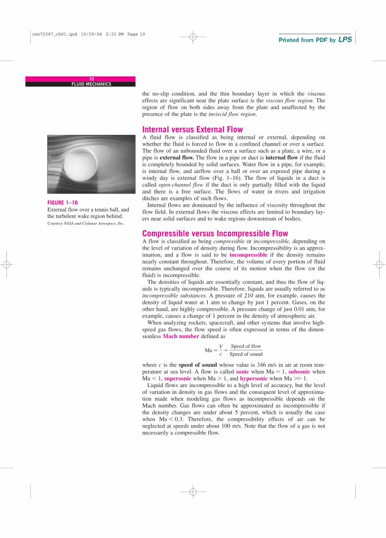
Internal versus External FlowA fluid flow is classified as being internal or external, depending onwhether the fluid is forced to flow in a confined channel or over a surface.The flow of an unbounded fluid over a surface such as a plate, a wire, or apipe is external flow. The flow in a pipe or duct is internal flow if the fluidis completely bounded by solid surfaces. Water flow in a pipe, for example,is internal flow, and airflow over a ball or over an exposed pipe during awindy day is external flow (Fig. 1–16). The flow of liquids in a duct iscalled open-channel flow if the duct is only partially filled with the liquidand there is a free surface. The flows of water in rivers and irrigationditches are examples of such flows.

Internal flows are dominated by the influence of viscosity throughout theflow field. In external flows the viscous effects are limited to boundary lay-ers near solid surfaces and to wake regions downstream of bodies.

Compressible versus Incompressible FlowA flow is classified as being compressible or incompressible, depending onthe level of variation of density during flow. Incompressibility is an approx-imation, and a flow is said to be incompressible if the density remainsnearly constant throughout. Therefore, the volume of every portion of fluidremains unchanged over the course of its motion when the flow (or thefluid) is incompressible.

The densities of liquids are essentially constant, and thus the flow of liq-uids is typically incompressible. Therefore, liquids are usually referred to asincompressible substances. A pressure of 210 atm, for example, causes thedensity of liquid water at 1 atm to change by just 1 percent. Gases, on theother hand, are highly compressible. A pressure change of just 0.01 atm, forexample, causes a change of 1 percent in the density of atmospheric air.

When analyzing rockets, spacecraft, and other systems that involve high-speed gas flows, the flow speed is often expressed in terms of the dimen-sionless Mach number defined as

where c is the speed of sound whose value is 346 m/s in air at room tem-perature at sea level. A flow is called sonic when Ma � 1, subsonic whenMa � 1, supersonic when Ma � 1, and hypersonic when Ma �� 1.

Liquid flows are incompressible to a high level of accuracy, but the levelof variation in density in gas flows and the consequent level of approxima-tion made when modeling gas flows as incompressible depends on theMach number. Gas flows can often be approximated as incompressible ifthe density changes are under about 5 percent, which is usually the casewhen Ma � 0.3. Therefore, the compressibility effects of air can beneglected at speeds under about 100 m/s. Note that the flow of a gas is notnecessarily a compressible flow.

Ma �V

c�

Speed of flow

Speed of sound

10FLUID MECHANICS

FIGURE 1–16

External flow over a tennis ball, andthe turbulent wake region behind.

Courtesy NASA and Cislunar Aerospace, Inc.

cen72367_ch01.qxd 10/29/04 2:32 PM

Small density changes of liquids corresponding to large pressure changescan still have important consequences. The irritating “water hammer” in awater pipe, for example, is caused by the vibrations of the pipe generated bythe reflection of pressure waves following the sudden closing of the valves.

Laminar versus Turbulent FlowSome flows are smooth and orderly while others are rather chaotic. Thehighly ordered fluid motion characterized by smooth layers of fluid is calledlaminar. The word laminar comes from the movement of adjacent fluidparticles together in “laminates.” The flow of high-viscosity fluids such asoils at low velocities is typically laminar. The highly disordered fluidmotion that typically occurs at high velocities and is characterized by veloc-ity fluctuations is called turbulent (Fig. 1–17). The flow of low-viscosityfluids such as air at high velocities is typically turbulent. The flow regimegreatly influences the required power for pumping. A flow that alternatesbetween being laminar and turbulent is called transitional. The experimentsconducted by Osborn Reynolds in the 1880s resulted in the establishment ofthe dimensionless Reynolds number, Re, as the key parameter for thedetermination of the flow regime in pipes (Chap. 8).

Natural (or Unforced) versus Forced FlowA fluid flow is said to be natural or forced, depending on how the fluidmotion is initiated. In forced flow, a fluid is forced to flow over a surface orin a pipe by external means such as a pump or a fan. In natural flows, anyfluid motion is due to natural means such as the buoyancy effect, whichmanifests itself as the rise of the warmer (and thus lighter) fluid and the fallof cooler (and thus denser) fluid (Fig. 1–18). In solar hot-water systems, forexample, the thermosiphoning effect is commonly used to replace pumps byplacing the water tank sufficiently above the solar collectors.

Steady versus Unsteady FlowThe terms steady and uniform are used frequently in engineering, and thus itis important to have a clear understanding of their meanings. The termsteady implies no change at a point with time. The opposite of steady isunsteady. The term uniform implies no change with location over a speci-fied region. These meanings are consistent with their everyday use (steadygirlfriend, uniform distribution, etc.).

The terms unsteady and transient are often used interchangeably, butthese terms are not synonyms. In fluid mechanics, unsteady is the most gen-eral term that applies to any flow that is not steady, but transient is typi-cally used for developing flows. When a rocket engine is fired up, for exam-ple, there are transient effects (the pressure builds up inside the rocketengine, the flow accelerates, etc.) until the engine settles down and operatessteadily. The term periodic refers to the kind of unsteady flow in which theflow oscillates about a steady mean.

Many devices such as turbines, compressors, boilers, condensers, and heatexchangers operate for long periods of time under the same conditions, andthey are classified as steady-flow devices. (Note that the flow field near therotating blades of a turbomachine is of course unsteady, but we consider theoverall flow field rather than the details at some localities when we classify

11CHAPTER 1

Laminar

Transitional

Turbulent

FIGURE 1–17

Laminar, transitional, and turbulentflows.

Courtesy ONERA, photograph by Werlé.

FIGURE 1–18

In this schlieren image of a girl in aswimming suit, the rise of lighter,

warmer air adjacent to her bodyindicates that humans and warm-

blooded animals are surrounded bythermal plumes of rising warm air.

G. S. Settles, Gas Dynamics Lab,

Penn State University. Used by permission.

cen72367_ch01.qxd 10/29/04 2:32 PM

devices.) During steady flow, the fluid properties can change from point topoint within a device, but at any fixed point they remain constant. There-fore, the volume, the mass, and the total energy content of a steady-flowdevice or flow section remain constant in steady operation.

Steady-flow conditions can be closely approximated by devices that areintended for continuous operation such as turbines, pumps, boilers, con-densers, and heat exchangers of power plants or refrigeration systems. Somecyclic devices, such as reciprocating engines or compressors, do not satisfythe steady-flow conditions since the flow at the inlets and the exits is pulsat-ing and not steady. However, the fluid properties vary with time in a peri-odic manner, and the flow through these devices can still be analyzed as asteady-flow process by using time-averaged values for the properties.

Some fascinating visualizations of fluid flow are provided in the book An

Album of Fluid Motion by Milton Van Dyke (1982). A nice illustration of anunsteady-flow field is shown in Fig. 1–19, taken from Van Dyke’s book.Figure 1–19a is an instantaneous snapshot from a high-speed motion pic-ture; it reveals large, alternating, swirling, turbulent eddies that are shed intothe periodically oscillating wake from the blunt base of the object. Theeddies produce shock waves that move upstream alternately over the top andbottom surfaces of the airfoil in an unsteady fashion. Figure 1–19b showsthe same flow field, but the film is exposed for a longer time so that theimage is time averaged over 12 cycles. The resulting time-averaged flowfield appears “steady” since the details of the unsteady oscillations havebeen lost in the long exposure.

One of the most important jobs of an engineer is to determine whether itis sufficient to study only the time-averaged “steady” flow features of aproblem, or whether a more detailed study of the unsteady features isrequired. If the engineer were interested only in the overall properties of theflow field, (such as the time-averaged drag coefficient, the mean velocity,and pressure fields) a time-averaged description like that of Fig. 1–19b,time-averaged experimental measurements, or an analytical or numericalcalculation of the time-averaged flow field would be sufficient. However, ifthe engineer were interested in details about the unsteady-flow field, such asflow-induced vibrations, unsteady pressure fluctuations, or the sound wavesemitted from the turbulent eddies or the shock waves, a time-averageddescription of the flow field would be insufficient.

Most of the analytical and computational examples provided in this text-book deal with steady or time-averaged flows, although we occasionallypoint out some relevant unsteady-flow features as well when appropriate.

One-, Two-, and Three-Dimensional FlowsA flow field is best characterized by the velocity distribution, and thus aflow is said to be one-, two-, or three-dimensional if the flow velocity variesin one, two, or three primary dimensions, respectively. A typical fluid flowinvolves a three-dimensional geometry, and the velocity may vary in allthree dimensions, rendering the flow three-dimensional [V

→

(x, y, z) in rec-tangular or V

→

(r, u, z) in cylindrical coordinates]. However, the variation ofvelocity in certain directions can be small relative to the variation in otherdirections and can be ignored with negligible error. In such cases, the flowcan be modeled conveniently as being one- or two-dimensional, which iseasier to analyze.

12FLUID MECHANICS

(a)

(b)

FIGURE 1–19

Oscillating wake of a blunt-basedairfoil at Mach number 0.6. Photo (a)is an instantaneous image, whilephoto (b) is a long-exposure (time-averaged) image.

(a) Dyment, A., Flodrops, J. P. & Gryson, P. 1982

in Flow Visualization II, W. Merzkirch, ed.,

331–336. Washington: Hemisphere. Used by

permission of Arthur Dyment.

(b) Dyment, A. & Gryson, P. 1978 in Inst. Mèc.

Fluides Lille, No. 78-5. Used by permission of

Arthur Dyment.

cen72367_ch01.qxd 10/29/04 2:32 PM

Consider steady flow of a fluid through a circular pipe attached to a largetank. The fluid velocity everywhere on the pipe surface is zero because ofthe no-slip condition, and the flow is two-dimensional in the entrance regionof the pipe since the velocity changes in both the r- and z-directions. Thevelocity profile develops fully and remains unchanged after some distancefrom the inlet (about 10 pipe diameters in turbulent flow, and less in laminarpipe flow, as in Fig. 1–20), and the flow in this region is said to be fully

developed. The fully developed flow in a circular pipe is one-dimensional

since the velocity varies in the radial r-direction but not in the angular u- oraxial z-directions, as shown in Fig. 1–20. That is, the velocity profile is thesame at any axial z-location, and it is symmetric about the axis of the pipe.

Note that the dimensionality of the flow also depends on the choice ofcoordinate system and its orientation. The pipe flow discussed, for example,is one-dimensional in cylindrical coordinates, but two-dimensional in Carte-sian coordinates—illustrating the importance of choosing the most appropri-ate coordinate system. Also note that even in this simple flow, the velocitycannot be uniform across the cross section of the pipe because of the no-slipcondition. However, at a well-rounded entrance to the pipe, the velocity pro-file may be approximated as being nearly uniform across the pipe, since thevelocity is nearly constant at all radii except very close to the pipe wall.

A flow may be approximated as two-dimensional when the aspect ratio islarge and the flow does not change appreciably along the longer dimension.For example, the flow of air over a car antenna can be considered two-dimen-sional except near its ends since the antenna’s length is much greater than itsdiameter, and the airflow hitting the antenna is fairly uniform (Fig. 1–21).

EXAMPLE 1–1 Axisymmetric Flow over a Bullet

Consider a bullet piercing through calm air. Determine if the time-averaged

airflow over the bullet during its flight is one-, two-, or three-dimensional (Fig.

1–22).

SOLUTION It is to be determined whether airflow over a bullet is one-, two-,

or three-dimensional.

Assumptions There are no significant winds and the bullet is not spinning.

Analysis The bullet possesses an axis of symmetry and is therefore an

axisymmetric body. The airflow upstream of the bullet is parallel to this axis,

and we expect the time-averaged airflow to be rotationally symmetric about

13CHAPTER 1

z

r

Developing velocity

profile, V(r, z)

Fully developed

velocity profile, V(r)

FIGURE 1–20

The development of the velocityprofile in a circular pipe. V � V(r, z)and thus the flow is two-dimensionalin the entrance region, and becomesone-dimensional downstream when

the velocity profile fully develops andremains unchanged in the flow

direction, V � V(r).

FIGURE 1–21

Flow over a car antenna isapproximately two-dimensional except near the top and bottom

of the antenna.

Axis ofsymmetry

r

zu

FIGURE 1–22

Axisymmetric flow over a bullet.

cen72367_ch01.qxd 10/29/04 2:32 PM

the axis—such flows are said to be axisymmetric. The velocity in this case

varies with axial distance z and radial distance r, but not with angle u.

Therefore, the time-averaged airflow over the bullet is two-dimensional.

Discussion While the time-averaged airflow is axisymmetric, the instanta-

neous airflow is not, as illustrated in Fig. 1–19.

1–5 � SYSTEM AND CONTROL VOLUME

A system is defined as a quantity of matter or a region in space chosen for

study. The mass or region outside the system is called the surroundings.

The real or imaginary surface that separates the system from its surround-ings is called the boundary (Fig. 1–23). The boundary of a system can befixed or movable. Note that the boundary is the contact surface shared byboth the system and the surroundings. Mathematically speaking, the bound-ary has zero thickness, and thus it can neither contain any mass nor occupyany volume in space.

Systems may be considered to be closed or open, depending on whether afixed mass or a volume in space is chosen for study. A closed system (alsoknown as a control mass) consists of a fixed amount of mass, and no masscan cross its boundary. But energy, in the form of heat or work, can crossthe boundary, and the volume of a closed system does not have to be fixed.If, as a special case, even energy is not allowed to cross the boundary, thatsystem is called an isolated system.

Consider the piston–cylinder device shown in Fig. 1–24. Let us say thatwe would like to find out what happens to the enclosed gas when it isheated. Since we are focusing our attention on the gas, it is our system. Theinner surfaces of the piston and the cylinder form the boundary, and sinceno mass is crossing this boundary, it is a closed system. Notice that energymay cross the boundary, and part of the boundary (the inner surface of thepiston, in this case) may move. Everything outside the gas, including thepiston and the cylinder, is the surroundings.

An open system, or a control volume, as it is often called, is a properlyselected region in space. It usually encloses a device that involves mass flowsuch as a compressor, turbine, or nozzle. Flow through these devices is beststudied by selecting the region within the device as the control volume.Both mass and energy can cross the boundary of a control volume.

A large number of engineering problems involve mass flow in and out ofa system and, therefore, are modeled as control volumes. A water heater, acar radiator, a turbine, and a compressor all involve mass flow and shouldbe analyzed as control volumes (open systems) instead of as control masses(closed systems). In general, any arbitrary region in space can be selectedas a control volume. There are no concrete rules for the selection of controlvolumes, but the proper choice certainly makes the analysis much easier. Ifwe were to analyze the flow of air through a nozzle, for example, a goodchoice for the control volume would be the region within the nozzle.

A control volume can be fixed in size and shape, as in the case of a noz-zle, or it may involve a moving boundary, as shown in Fig. 1–25. Most con-trol volumes, however, have fixed boundaries and thus do not involve any

14FLUID MECHANICS

SURROUNDINGS

BOUNDARY

SYSTEM

FIGURE 1–23

System, surroundings, and boundary.

GAS

2 kg

1.5 m3GAS

2 kg

1 m3

Movingboundary

Fixedboundary

FIGURE 1–24

A closed system with a movingboundary.

cen72367_ch01.qxd 10/29/04 2:32 PM

moving boundaries. A control volume may also involve heat and work inter-actions just as a closed system, in addition to mass interaction.

1–6 � IMPORTANCE OF DIMENSIONS AND UNITS

Any physical quantity can be characterized by dimensions. The magnitudesassigned to the dimensions are called units. Some basic dimensions such asmass m, length L, time t, and temperature T are selected as primary or fun-

damental dimensions, while others such as velocity V, energy E, and vol-ume V are expressed in terms of the primary dimensions and are called sec-

ondary dimensions, or derived dimensions.

A number of unit systems have been developed over the years. Despitestrong efforts in the scientific and engineering community to unify theworld with a single unit system, two sets of units are still in common usetoday: the English system, which is also known as the United States Cus-

tomary System (USCS), and the metric SI (from Le Système International

d’ Unités), which is also known as the International System. The SI is a sim-ple and logical system based on a decimal relationship between the variousunits, and it is being used for scientific and engineering work in most of theindustrialized nations, including England. The English system, however, hasno apparent systematic numerical base, and various units in this system arerelated to each other rather arbitrarily (12 in � 1 ft, 1 mile � 5280 ft, 4 qt� 1 gal, etc.), which makes it confusing and difficult to learn. The UnitedStates is the only industrialized country that has not yet fully converted tothe metric system.

The systematic efforts to develop a universally acceptable system of unitsdates back to 1790 when the French National Assembly charged the FrenchAcademy of Sciences to come up with such a unit system. An early versionof the metric system was soon developed in France, but it did not find uni-versal acceptance until 1875 when The Metric Convention Treaty was pre-pared and signed by 17 nations, including the United States. In this interna-tional treaty, meter and gram were established as the metric units for lengthand mass, respectively, and a General Conference of Weights and Measures

(CGPM) was established that was to meet every six years. In 1960, the

15CHAPTER 1

CV

Movingboundary

Fixedboundary

CV

(a nozzle)

Real boundary

(b) A control volume (CV) with fixed and

moving boundaries

(a) A control volume (CV) with real and

imaginary boundaries

Imaginaryboundary

FIGURE 1–25

A control volume may involve fixed,moving, real, and imaginary

boundaries.

cen72367_ch01.qxd 10/29/04 2:32 PM

CGPM produced the SI, which was based on six fundamental quantities,and their units were adopted in 1954 at the Tenth General Conference ofWeights and Measures: meter (m) for length, kilogram (kg) for mass, sec-

ond (s) for time, ampere (A) for electric current, degree Kelvin (°K) fortemperature, and candela (cd) for luminous intensity (amount of light). In1971, the CGPM added a seventh fundamental quantity and unit: mole

(mol) for the amount of matter.Based on the notational scheme introduced in 1967, the degree symbol

was officially dropped from the absolute temperature unit, and all unitnames were to be written without capitalization even if they were derivedfrom proper names (Table 1–1). However, the abbreviation of a unit was tobe capitalized if the unit was derived from a proper name. For example, theSI unit of force, which is named after Sir Isaac Newton (1647–1723), isnewton (not Newton), and it is abbreviated as N. Also, the full name of aunit may be pluralized, but its abbreviation cannot. For example, the lengthof an object can be 5 m or 5 meters, not 5 ms or 5 meter. Finally, no periodis to be used in unit abbreviations unless they appear at the end of a sen-tence. For example, the proper abbreviation of meter is m (not m.).

The recent move toward the metric system in the United States seems tohave started in 1968 when Congress, in response to what was happening inthe rest of the world, passed a Metric Study Act. Congress continued to pro-mote a voluntary switch to the metric system by passing the Metric Conver-sion Act in 1975. A trade bill passed by Congress in 1988 set a September1992 deadline for all federal agencies to convert to the metric system. How-ever, the deadlines were relaxed later with no clear plans for the future.

The industries that are heavily involved in international trade (such as theautomotive, soft drink, and liquor industries) have been quick in convertingto the metric system for economic reasons (having a single worldwidedesign, fewer sizes, smaller inventories, etc.). Today, nearly all the carsmanufactured in the United States are metric. Most car owners probably donot realize this until they try an English socket wrench on a metric bolt.Most industries, however, resisted the change, thus slowing down the con-version process.

Presently the United States is a dual-system society, and it will stay thatway until the transition to the metric system is completed. This puts an extraburden on today’s engineering students, since they are expected to retaintheir understanding of the English system while learning, thinking, andworking in terms of the SI. Given the position of the engineers in the transi-tion period, both unit systems are used in this text, with particular emphasison SI units.

As pointed out, the SI is based on a decimal relationship between units.The prefixes used to express the multiples of the various units are listed inTable 1–2. They are standard for all units, and the student is encouraged tomemorize them because of their widespread use (Fig. 1–26).

Some SI and English UnitsIn SI, the units of mass, length, and time are the kilogram (kg), meter (m),and second (s), respectively. The respective units in the English system arethe pound-mass (lbm), foot (ft), and second (s). The pound symbol lb is

16FLUID MECHANICS

TABLE 1–1

The seven fundamental (or primary)

dimensions and their units in SI

Dimension Unit

Length meter (m)

Mass kilogram (kg)

Time second (s)

Temperature kelvin (K)

Electric current ampere (A)

Amount of light candela (cd)

Amount of matter mole (mol)

TABLE 1–2

Standard prefixes in SI units

Multiple Prefix

1012 tera, T

109 giga, G

106 mega, M

103 kilo, k

102 hecto, h

101 deka, da

10�1 deci, d

10�2 centi, c

10�3 milli, m

10�6 micro, m

10�9 nano, n

10�12 pico, p

cen72367_ch01.qxd 10/29/04 2:32 PM

actually the abbreviation of libra, which was the ancient Roman unit ofweight. The English retained this symbol even after the end of the Romanoccupation of Britain in 410. The mass and length units in the two systemsare related to each other by

In the English system, force is usually considered to be one of the pri-mary dimensions and is assigned a nonderived unit. This is a source of con-fusion and error that necessitates the use of a dimensional constant (gc) inmany formulas. To avoid this nuisance, we consider force to be a secondarydimension whose unit is derived from Newton’s second law, i.e.,

Force � (Mass) (Acceleration)

or F � ma (1–1)

In SI, the force unit is the newton (N), and it is defined as the force required

to accelerate a mass of 1 kg at a rate of 1 m/s2. In the English system, theforce unit is the pound-force (lbf) and is defined as the force required to

accelerate a mass of 32.174 lbm (1 slug) at a rate of 1 ft/s2 (Fig. 1–27).That is,

A force of 1 N is roughly equivalent to the weight of a small apple (m� 102 g), whereas a force of 1 lbf is roughly equivalent to the weight offour medium apples (mtotal � 454 g), as shown in Fig. 1–28. Another forceunit in common use in many European countries is the kilogram-force (kgf),which is the weight of 1 kg mass at sea level (1 kgf � 9.807 N).

The term weight is often incorrectly used to express mass, particularly bythe “weight watchers.” Unlike mass, weight W is a force. It is the gravita-tional force applied to a body, and its magnitude is determined from New-ton’s second law,

(1–2)

where m is the mass of the body, and g is the local gravitational acceleration(g is 9.807 m/s2 or 32.174 ft/s2 at sea level and 45° latitude). An ordinarybathroom scale measures the gravitational force acting on a body. Theweight of a unit volume of a substance is called the specific weight g and isdetermined from g� rg, where r is density.

The mass of a body remains the same regardless of its location in the uni-verse. Its weight, however, changes with a change in gravitational accelera-tion. A body weighs less on top of a mountain since g decreases with altitude.

W � mg (N)

1 lbf � 32.174 lbm � ft/s2

1 N � 1 kg � m/s2

1 ft � 0.3048 m

1 lbm � 0.45359 kg

17CHAPTER 1

200 mL(0.2 L)

1 kg(103 g)

1 M�

(106 �)

FIGURE 1–26

The SI unit prefixes are used in allbranches of engineering.

m = 1 kg

m = 32.174 lbm

a = 1 m/s 2

a = 1 ft/s 2

F = 1 lbf

F = 1 N

FIGURE 1–27

The definition of the force units.

1 kgf

10 apples

m = 1 kg

4 apples

m = 1 lbm

1 lbf

1 apple

m = 102 g

1 N

FIGURE 1–28

The relative magnitudes of the forceunits newton (N), kilogram-force

(kgf), and pound-force (lbf).

cen72367_ch01.qxd 10/29/04 2:32 PM

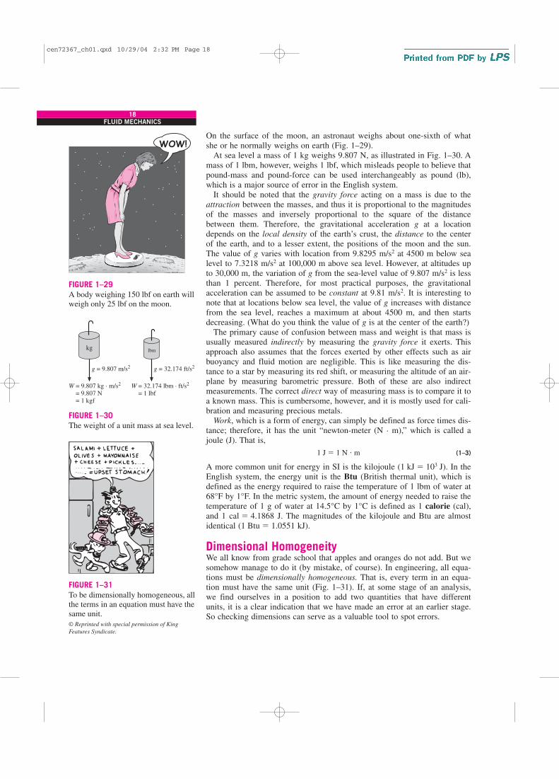
On the surface of the moon, an astronaut weighs about one-sixth of whatshe or he normally weighs on earth (Fig. 1–29).

At sea level a mass of 1 kg weighs 9.807 N, as illustrated in Fig. 1–30. Amass of 1 lbm, however, weighs 1 lbf, which misleads people to believe thatpound-mass and pound-force can be used interchangeably as pound (lb),which is a major source of error in the English system.

It should be noted that the gravity force acting on a mass is due to theattraction between the masses, and thus it is proportional to the magnitudesof the masses and inversely proportional to the square of the distancebetween them. Therefore, the gravitational acceleration g at a locationdepends on the local density of the earth’s crust, the distance to the centerof the earth, and to a lesser extent, the positions of the moon and the sun.The value of g varies with location from 9.8295 m/s2 at 4500 m below sealevel to 7.3218 m/s2 at 100,000 m above sea level. However, at altitudes upto 30,000 m, the variation of g from the sea-level value of 9.807 m/s2 is lessthan 1 percent. Therefore, for most practical purposes, the gravitationalacceleration can be assumed to be constant at 9.81 m/s2. It is interesting tonote that at locations below sea level, the value of g increases with distancefrom the sea level, reaches a maximum at about 4500 m, and then startsdecreasing. (What do you think the value of g is at the center of the earth?)

The primary cause of confusion between mass and weight is that mass isusually measured indirectly by measuring the gravity force it exerts. Thisapproach also assumes that the forces exerted by other effects such as airbuoyancy and fluid motion are negligible. This is like measuring the dis-tance to a star by measuring its red shift, or measuring the altitude of an air-plane by measuring barometric pressure. Both of these are also indirectmeasurements. The correct direct way of measuring mass is to compare it toa known mass. This is cumbersome, however, and it is mostly used for cali-bration and measuring precious metals.

Work, which is a form of energy, can simply be defined as force times dis-tance; therefore, it has the unit “newton-meter (N . m),” which is called ajoule (J). That is,

(1–3)

A more common unit for energy in SI is the kilojoule (1 kJ � 103 J). In theEnglish system, the energy unit is the Btu (British thermal unit), which isdefined as the energy required to raise the temperature of 1 lbm of water at68°F by 1°F. In the metric system, the amount of energy needed to raise thetemperature of 1 g of water at 14.5°C by 1°C is defined as 1 calorie (cal),and 1 cal � 4.1868 J. The magnitudes of the kilojoule and Btu are almostidentical (1 Btu � 1.0551 kJ).

Dimensional HomogeneityWe all know from grade school that apples and oranges do not add. But wesomehow manage to do it (by mistake, of course). In engineering, all equa-tions must be dimensionally homogeneous. That is, every term in an equa-tion must have the same unit (Fig. 1–31). If, at some stage of an analysis,we find ourselves in a position to add two quantities that have differentunits, it is a clear indication that we have made an error at an earlier stage.So checking dimensions can serve as a valuable tool to spot errors.

1 J � 1 N � m

18FLUID MECHANICS

FIGURE 1–29

A body weighing 150 lbf on earth willweigh only 25 lbf on the moon.

g = 9.807 m/s2

W = 9.807 kg · m/s2

= 9.807 N = 1 kgf

W = 32.174 lbm · ft/s2

= 1 lbf

g = 32.174 ft/s2

kg lbm

FIGURE 1–30

The weight of a unit mass at sea level.

FIGURE 1–31

To be dimensionally homogeneous, allthe terms in an equation must have thesame unit.

© Reprinted with special permission of King

Features Syndicate.

cen72367_ch01.qxd 10/29/04 2:32 PM

EXAMPLE 1–2 Spotting Errors from Unit Inconsistencies

While solving a problem, a person ended up with the following equation at

some stage:

where E is the total energy and has the unit of kilojoules. Determine how to

correct the error and discuss what may have caused it.

SOLUTION During an analysis, a relation with inconsistent units is obtained.

A correction is to be found, and the probable cause of the error is to be

determined.

Analysis The two terms on the right-hand side do not have the same units,

and therefore they cannot be added to obtain the total energy. Multiplying

the last term by mass will eliminate the kilograms in the denominator, and

the whole equation will become dimensionally homogeneous; that is, every

term in the equation will have the same unit.

Discussion Obviously this error was caused by forgetting to multiply the last

term by mass at an earlier stage.

We all know from experience that units can give terrible headaches if theyare not used carefully in solving a problem. However, with some attentionand skill, units can be used to our advantage. They can be used to check for-mulas; they can even be used to derive formulas, as explained in the follow-ing example.

EXAMPLE 1–3 Obtaining Formulas from Unit Considerations

A tank is filled with oil whose density is r� 850 kg/m3. If the volume of the

tank is V � 2 m3, determine the amount of mass m in the tank.

SOLUTION The volume of an oil tank is given. The mass of oil is to be

determined.

Assumptions Oil is an incompressible substance and thus its density is

constant.

Analysis A sketch of the system just described is given in Fig. 1–32. Sup-

pose we forgot the formula that relates mass to density and volume. However,

we know that mass has the unit of kilograms. That is, whatever calculations

we do, we should end up with the unit of kilograms. Putting the given infor-

mation into perspective, we have

It is obvious that we can eliminate m3 and end up with kg by multiplying

these two quantities. Therefore, the formula we are looking for should be

Thus,

Discussion Note that this approach may not work for more complicated

formulas.

m � (850 kg/m3)(2 m3) � 1700 kg

m � rV

r � 850 kg/m3 and V � 2 m3

E � 25 kJ � 7 kJ/kg

19CHAPTER 1

V = 2 m3

ρ = 850 kg/m3

m = ?

OIL

FIGURE 1–32

Schematic for Example 1–3.

cen72367_ch01.qxd 10/29/04 2:32 PM

20FLUID MECHANICS

lbm

FIGURE 1–33

A mass of 1 lbm weighs 1 lbf on earth.

The student should keep in mind that a formula that is not dimensionallyhomogeneous is definitely wrong, but a dimensionally homogeneous for-mula is not necessarily right.

Unity Conversion RatiosJust as all nonprimary dimensions can be formed by suitable combinationsof primary dimensions, all nonprimary units (secondary units) can be

formed by combinations of primary units. Force units, for example, can beexpressed as

They can also be expressed more conveniently as unity conversion ratios as

Unity conversion ratios are identically equal to 1 and are unitless, and thussuch ratios (or their inverses) can be inserted conveniently into any calcula-tion to properly convert units. Students are encouraged to always use unityconversion ratios such as those given here when converting units. Some text-books insert the archaic gravitational constant gc defined as gc � 32.174 lbm· ft/lbf · s2 � kg · m/N · s2 � 1 into equations in order to force units tomatch. This practice leads to unnecessary confusion and is strongly discour-aged by the present authors. We recommend that students instead use unityconversion ratios.

EXAMPLE 1–4 The Weight of One Pound-Mass

Using unity conversion ratios, show that 1.00 lbm weighs 1.00 lbf on earth

(Fig. 1–33).

Solution A mass of 1.00 lbm is subjected to standard earth gravity. Its

weight in lbf is to be determined.

Assumptions Standard sea-level conditions are assumed.

Properties The gravitational constant is g � 32.174 ft/s2.Analysis We apply Newton’s second law to calculate the weight (force) that

corresponds to the known mass and acceleration. The weight of any object is

equal to its mass times the local value of gravitational acceleration. Thus,

Discussion Mass is the same regardless of its location. However, on some

other planet with a different value of gravitational acceleration, the weight of

1 lbm would differ from that calculated here.

When you buy a box of breakfast cereal, the printing may say “Netweight: One pound (454 grams).” (See Fig. 1–34.) Technically, this meansthat the cereal inside the box weighs 1.00 lbf on earth and has a mass of

W � mg � (1.00 lbm)(32.174 ft/s2)a 1 lbf

32.174 lbm � ft/s2b � 1.00 lbf

N

kg � m/s2� 1 and

lbf

32.174 lbm � ft/s2� 1

N � kg m

s2 and lbf � 32.174 lbm

ft

s2

cen72367_ch01.qxd 10/29/04 2:32 PM

453.6 gm (0.4536 kg). Using Newton’s second law, the actual weight onearth of the cereal in the metric system is

1–7 � MATHEMATICAL MODELING OF ENGINEERING PROBLEMS

An engineering device or process can be studied either experimentally (test-ing and taking measurements) or analytically (by analysis or calculations).The experimental approach has the advantage that we deal with the actualphysical system, and the desired quantity is determined by measurement,within the limits of experimental error. However, this approach is expensive,time-consuming, and often impractical. Besides, the system we are studyingmay not even exist. For example, the entire heating and plumbing systemsof a building must usually be sized before the building is actually built onthe basis of the specifications given. The analytical approach (including thenumerical approach) has the advantage that it is fast and inexpensive, butthe results obtained are subject to the accuracy of the assumptions, approxi-mations, and idealizations made in the analysis. In engineering studies,often a good compromise is reached by reducing the choices to just a fewby analysis, and then verifying the findings experimentally.

Modeling in EngineeringThe descriptions of most scientific problems involve equations that relatethe changes in some key variables to each other. Usually the smaller theincrement chosen in the changing variables, the more general and accuratethe description. In the limiting case of infinitesimal or differential changesin variables, we obtain differential equations that provide precise mathemat-ical formulations for the physical principles and laws by representing therates of change as derivatives. Therefore, differential equations are used toinvestigate a wide variety of problems in sciences and engineering (Fig.1–35). However, many problems encountered in practice can be solvedwithout resorting to differential equations and the complications associatedwith them.

The study of physical phenomena involves two important steps. In thefirst step, all the variables that affect the phenomena are identified, reason-able assumptions and approximations are made, and the interdependence ofthese variables is studied. The relevant physical laws and principles areinvoked, and the problem is formulated mathematically. The equation itselfis very instructive as it shows the degree of dependence of some variableson others, and the relative importance of various terms. In the second step,the problem is solved using an appropriate approach, and the results areinterpreted.

Many processes that seem to occur in nature randomly and without anyorder are, in fact, being governed by some visible or not-so-visible physicallaws. Whether we notice them or not, these laws are there, governing con-sistently and predictably over what seem to be ordinary events. Most of

W � mg � (453.6 g)(9.81 m/s2)a 1 N

1 kg � m/s2b a 1 kg

1000 gb � 4.49 N

21CHAPTER 1

Net weight:One pound (454 grams)

FIGURE 1–34

A quirk in the metric system of units.

Identifyimportantvariables Make

reasonableassumptions andapproximationsApply

relevantphysical laws

Physical problem

A differential equation

Applyapplicablesolution

technique

Applyboundaryand initialconditions

Solution of the problem

FIGURE 1–35

Mathematical modeling of physicalproblems.

cen72367_ch01.qxd 10/29/04 2:32 PM

these laws are well defined and well understood by scientists. This makes itpossible to predict the course of an event before it actually occurs or tostudy various aspects of an event mathematically without actually runningexpensive and time-consuming experiments. This is where the power ofanalysis lies. Very accurate results to meaningful practical problems can beobtained with relatively little effort by using a suitable and realistic mathe-matical model. The preparation of such models requires an adequate knowl-edge of the natural phenomena involved and the relevant laws, as well assound judgment. An unrealistic model will obviously give inaccurate andthus unacceptable results.

An analyst working on an engineering problem often finds himself or her-self in a position to make a choice between a very accurate but complexmodel, and a simple but not-so-accurate model. The right choice depends onthe situation at hand. The right choice is usually the simplest model thatyields satisfactory results. Also, it is important to consider the actual operat-ing conditions when selecting equipment.

Preparing very accurate but complex models is usually not so difficult.But such models are not much use to an analyst if they are very difficult andtime-consuming to solve. At the minimum, the model should reflect theessential features of the physical problem it represents. There are many sig-nificant real-world problems that can be analyzed with a simple model. Butit should always be kept in mind that the results obtained from an analysisare at best as accurate as the assumptions made in simplifying the problem.Therefore, the solution obtained should not be applied to situations forwhich the original assumptions do not hold.

A solution that is not quite consistent with the observed nature of the prob-lem indicates that the mathematical model used is too crude. In that case, amore realistic model should be prepared by eliminating one or more of thequestionable assumptions. This will result in a more complex problem that,of course, is more difficult to solve. Thus any solution to a problem shouldbe interpreted within the context of its formulation.

1–8 � PROBLEM-SOLVING TECHNIQUE

The first step in learning any science is to grasp the fundamentals and to gaina sound knowledge of it. The next step is to master the fundamentals by test-ing this knowledge. This is done by solving significant real-world problems.Solving such problems, especially complicated ones, requires a systematicapproach. By using a step-by-step approach, an engineer can reduce the solu-tion of a complicated problem into the solution of a series of simple prob-lems (Fig. 1–36). When you are solving a problem, we recommend that youuse the following steps zealously as applicable. This will help you avoidsome of the common pitfalls associated with problem solving.

Step 1: Problem StatementIn your own words, briefly state the problem, the key information given,and the quantities to be found. This is to make sure that you understand theproblem and the objectives before you attempt to solve the problem.

22FLUID MECHANICS

SOLUTION

PROBLEM

HA

RD

WA

Y

EASY WAY

FIGURE 1–36

A step-by-step approach can greatlysimplify problem solving.

cen72367_ch01.qxd 10/29/04 2:32 PM

Step 2: SchematicDraw a realistic sketch of the physical system involved, and list the relevantinformation on the figure. The sketch does not have to be something elabo-rate, but it should resemble the actual system and show the key features.Indicate any energy and mass interactions with the surroundings. Listing thegiven information on the sketch helps one to see the entire problem at once.Also, check for properties that remain constant during a process (such astemperature during an isothermal process), and indicate them on the sketch.

Step 3: Assumptions and ApproximationsState any appropriate assumptions and approximations made to simplify theproblem to make it possible to obtain a solution. Justify the questionableassumptions. Assume reasonable values for missing quantities that are nec-essary. For example, in the absence of specific data for atmospheric pres-sure, it can be taken to be 1 atm. However, it should be noted in the analysisthat the atmospheric pressure decreases with increasing elevation. For exam-ple, it drops to 0.83 atm in Denver (elevation 1610 m) (Fig. 1–37).

Step 4: Physical LawsApply all the relevant basic physical laws and principles (such as the con-servation of mass), and reduce them to their simplest form by utilizing theassumptions made. However, the region to which a physical law is appliedmust be clearly identified first. For example, the increase in speed of waterflowing through a nozzle is analyzed by applying conservation of massbetween the inlet and outlet of the nozzle.

Step 5: PropertiesDetermine the unknown properties at known states necessary to solve theproblem from property relations or tables. List the properties separately, andindicate their source, if applicable.

Step 6: CalculationsSubstitute the known quantities into the simplified relations and perform thecalculations to determine the unknowns. Pay particular attention to the unitsand unit cancellations, and remember that a dimensional quantity without aunit is meaningless. Also, don’t give a false implication of high precision bycopying all the digits from the screen of the calculator—round the results toan appropriate number of significant digits (Section 1–10).

Step 7: Reasoning, Verification, and DiscussionCheck to make sure that the results obtained are reasonable and intuitive,and verify the validity of the questionable assumptions. Repeat the calcula-tions that resulted in unreasonable values. For example, under the same testconditions the aerodynamic drag acting on a car should not increase afterstreamlining the shape of the car (Fig. 1–38).

Also, point out the significance of the results, and discuss their implica-tions. State the conclusions that can be drawn from the results, and any rec-ommendations that can be made from them. Emphasize the limitations

23CHAPTER 1

Given: Air temperature in Denver

To be found: Density of air

Missing information: Atmospheric

pressure

Assumption #1: Take P = 1 atm

(Inappropriate. Ignores effect of

altitude. Will cause more than

15% error.)

Assumption #2: Take P = 0.83 atm

(Appropriate. Ignores only minor

effects such as weather.)

FIGURE 1–37

The assumptions made while solvingan engineering problem must be

reasonable and justifiable.

Before streamliningV

VAfter streamliningUnreasonable!

FD

FD

FIGURE 1–38

The results obtained from anengineering analysis must be checked

for reasonableness.

cen72367_ch01.qxd 10/29/04 2:32 PM

under which the results are applicable, and caution against any possible mis-understandings and using the results in situations where the underlyingassumptions do not apply. For example, if you determined that using alarger-diameter pipe in a proposed pipeline will cost an additional $5000 inmaterials, but it will reduce the annual pumping costs by $3000, indicatethat the larger-diameter pipeline will pay for its cost differential from theelectricity it saves in less than two years. However, also state that only addi-tional material costs associated with the larger-diameter pipeline are consid-ered in the analysis.

Keep in mind that the solutions you present to your instructors, and anyengineering analysis presented to others, is a form of communication.Therefore neatness, organization, completeness, and visual appearance areof utmost importance for maximum effectiveness. Besides, neatness alsoserves as a great checking tool since it is very easy to spot errors and incon-sistencies in neat work. Carelessness and skipping steps to save time oftenend up costing more time and unnecessary anxiety.

The approach described here is used in the solved example problems with-out explicitly stating each step, as well as in the Solutions Manual of thistext. For some problems, some of the steps may not be applicable or neces-sary. For example, often it is not practical to list the properties separately.However, we cannot overemphasize the importance of a logical and orderlyapproach to problem solving. Most difficulties encountered while solving aproblem are not due to a lack of knowledge; rather, they are due to a lack oforganization. You are strongly encouraged to follow these steps in problemsolving until you develop your own approach that works best for you.

1–9 � ENGINEERING SOFTWARE PACKAGES

You may be wondering why we are about to undertake an in-depth study ofthe fundamentals of another engineering science. After all, almost all suchproblems we are likely to encounter in practice can be solved using one ofseveral sophisticated software packages readily available in the markettoday. These software packages not only give the desired numerical results,but also supply the outputs in colorful graphical form for impressive presen-tations. It is unthinkable to practice engineering today without using someof these packages. This tremendous computing power available to us at thetouch of a button is both a blessing and a curse. It certainly enables engi-neers to solve problems easily and quickly, but it also opens the door forabuses and misinformation. In the hands of poorly educated people, thesesoftware packages are as dangerous as sophisticated powerful weapons inthe hands of poorly trained soldiers.

Thinking that a person who can use the engineering software packageswithout proper training on fundamentals can practice engineering is likethinking that a person who can use a wrench can work as a car mechanic. Ifit were true that the engineering students do not need all these fundamentalcourses they are taking because practically everything can be done by com-puters quickly and easily, then it would also be true that the employers wouldno longer need high-salaried engineers since any person who knows how touse a word-processing program can also learn how to use those softwarepackages. However, the statistics show that the need for engineers is on therise, not on the decline, despite the availability of these powerful packages.

24FLUID MECHANICS

cen72367_ch01.qxd 10/29/04 2:32 PM

We should always remember that all the computing power and the engi-neering software packages available today are just tools, and tools havemeaning only in the hands of masters. Having the best word-processing pro-gram does not make a person a good writer, but it certainly makes the job ofa good writer much easier and makes the writer more productive (Fig.1–39). Hand calculators did not eliminate the need to teach our childrenhow to add or subtract, and the sophisticated medical software packages didnot take the place of medical school training. Neither will engineering soft-ware packages replace the traditional engineering education. They will sim-ply cause a shift in emphasis in the courses from mathematics to physics.That is, more time will be spent in the classroom discussing the physicalaspects of the problems in greater detail, and less time on the mechanics ofsolution procedures.

All these marvelous and powerful tools available today put an extra bur-den on today’s engineers. They must still have a thorough understanding ofthe fundamentals, develop a “feel” of the physical phenomena, be able toput the data into proper perspective, and make sound engineering judg-ments, just like their predecessors. However, they must do it much better,and much faster, using more realistic models because of the powerful toolsavailable today. The engineers in the past had to rely on hand calculations,slide rules, and later hand calculators and computers. Today they rely onsoftware packages. The easy access to such power and the possibility of asimple misunderstanding or misinterpretation causing great damage make itmore important today than ever to have solid training in the fundamentals ofengineering. In this text we make an extra effort to put the emphasis ondeveloping an intuitive and physical understanding of natural phenomenainstead of on the mathematical details of solution procedures.

Engineering Equation Solver (EES)EES is a program that solves systems of linear or nonlinear algebraic or dif-ferential equations numerically. It has a large library of built-in thermody-namic property functions as well as mathematical functions, and allows theuser to supply additional property data. Unlike some software packages,EES does not solve engineering problems; it only solves the equations sup-plied by the user. Therefore, the user must understand the problem and for-mulate it by applying any relevant physical laws and relations. EES savesthe user considerable time and effort by simply solving the resulting mathe-matical equations. This makes it possible to attempt significant engineeringproblems not suitable for hand calculations and to conduct parametric stud-ies quickly and conveniently. EES is a very powerful yet intuitive programthat is very easy to use, as shown in Example 1–5. The use and capabilitiesof EES are explained in Appendix 3 on the enclosed DVD.

EXAMPLE 1–5 Solving a System of Equations with EES

The difference of two numbers is 4, and the sum of the squares of these two

numbers is equal to the sum of the numbers plus 20. Determine these two

numbers.

25CHAPTER 1

Attached is a pdf of the text with windows and approx sizes for the art.

I'll give you rough ideas on the art, though you may have some differentthoughts on approaching these.

Fig 1 - 41 x 30The boxes fall into 2 columns, Type 1/2 on left and Type 1 on right.Nonenzymatic glycation is in the middle, between columns. Oxidative Stressand Axonal Degeneration are common outcomes and should be centered at thebottom beneath both columns (no need to stack them as shown). I wish I knewwhat the Polyol Pathway was, cause I'd like to illustrate it somehow.

Fig 2 -- 41 x 26This one's kinda straighforward, though I'd push Type 1/2 and Hyperglycemiafurther to the left, so that everything falls roughly under the other, Type1 column.

FIGURE 1–39

An excellent word-processingprogram does not make a person a good writer; it simply makes a

good writer a more efficient writer.

cen72367_ch01.qxd 10/29/04 2:32 PM

SOLUTION Relations are given for the difference and the sum of the

squares of two numbers. They are to be determined.

Analysis We start the EES program by double-clicking on its icon, open a

new file, and type the following on the blank screen that appears:

which is an exact mathematical expression of the problem statement with x

and y denoting the unknown numbers. The solution to this system of two

nonlinear equations with two unknowns is obtained by a single click on the

“calculator” icon on the taskbar. It gives

Discussion Note that all we did is formulate the problem as we would on

paper; EES took care of all the mathematical details of solution. Also note

that equations can be linear or nonlinear, and they can be entered in any

order with unknowns on either side. Friendly equation solvers such as EES

allow the user to concentrate on the physics of the problem without worrying

about the mathematical complexities associated with the solution of the

resulting system of equations.

FLUENTFLUENT is a computational fluid dynamics (CFD) code widely used forflow-modeling applications. The first step in analysis is preprocessing,which involves building a model or importing one from a CAD package,applying a finite-volume-based mesh, and entering data. Once the numericalmodel is prepared, FLUENT performs the necessary calculations and pro-duces the desired results. The final step in analysis is postprocessing, whichinvolves organization and interpretation of the data and images. Packagestailored for specific applications such as electronics cooling, ventilating sys-tems, and mixing are also available. FLUENT can handle subsonic or super-sonic flows, steady or transient flows, laminar or turbulent flows, Newton-ian or non-Newtonian flows, single or multiphase flows, chemical reactionsincluding combustion, flow through porous media, heat transfer, and flow-induced vibrations. Most numerical solutions presented in this text areobtained using FLUENT, and CFD is discussed in more detail in Chap. 15.

1–10 � ACCURACY, PRECISION, AND SIGNIFICANT DIGITS

In engineering calculations, the supplied information is not known to morethan a certain number of significant digits, usually three digits. Conse-quently, the results obtained cannot possibly be precise to more significantdigits. Reporting results in more significant digits implies greater precisionthan exists, and it should be avoided.

Regardless of the system of units employed, engineers must be aware ofthree principles that govern the proper use of numbers: accuracy, precision,

x�5 and y�1

xˆ2�yˆ2�x�y�20

x–y�4

26FLUID MECHANICS

cen72367_ch01.qxd 10/29/04 2:32 PM

and significant digits. For engineering measurements, they are defined asfollows:

• Accuracy error (inaccuracy) is the value of one reading minus the truevalue. In general, accuracy of a set of measurements refers to thecloseness of the average reading to the true value. Accuracy is generallyassociated with repeatable, fixed errors.

• Precision error is the value of one reading minus the average of readings. In

general, precision of a set of measurements refers to the fineness of the

resolution and the repeatability of the instrument. Precision is generally

associated with unrepeatable, random errors.

• Significant digits are digits that are relevant and meaningful.

A measurement or calculation can be very precise without being veryaccurate, and vice versa. For example, suppose the true value of wind speedis 25.00 m/s. Two anemometers A and B take five wind speed readings each:

Anemometer A: 25.50, 25.69, 25.52, 25.58, and 25.61 m/s. Average of all

readings � 25.58 m/s.

Anemometer B: 26.3, 24.5, 23.9, 26.8, and 23.6 m/s. Average of all readings

� 25.02 m/s.

Clearly, anemometer A is more precise, since none of the readings differsby more than 0.11 m/s from the average. However, the average is 25.58 m/s,0.58 m/s greater than the true wind speed; this indicates significant bias

error, also called constant error or systematic error. On the other hand,anemometer B is not very precise, since its readings swing wildly from theaverage; but its overall average is much closer to the true value. Hence,anemometer B is more accurate than anemometer A, at least for this set ofreadings, even though it is less precise. The difference between accuracyand precision can be illustrated effectively by analogy to shooting a gun at atarget, as sketched in Fig. 1–40. Shooter A is very precise, but not veryaccurate, while shooter B has better overall accuracy, but less precision.

Many engineers do not pay proper attention to the number of significantdigits in their calculations. The least significant numeral in a numberimplies the precision of the measurement or calculation. For example, aresult written as 1.23 (three significant digits) implies that the result is pre-cise to within one digit in the second decimal place; i.e., the number issomewhere between 1.22 and 1.24. Expressing this number with any moredigits would be misleading. The number of significant digits is most easilyevaluated when the number is written in exponential notation; the number ofsignificant digits can then simply be counted, including zeroes. Some exam-ples are shown in Table 1–3.

When performing calculations or manipulations of several parameters,the final result is generally only as precise as the least precise parameter inthe problem. For example, suppose A and B are multiplied to obtain C. If A � 2.3601 (five significant digits), and B � 0.34 (two significant digits),then C � 0.80 (only two digits are significant in the final result). Note thatmost students are tempted to write C � 0.802434, with six significant dig-its, since that is what is displayed on a calculator after multiplying thesetwo numbers.

27CHAPTER 1

A

B

+++

++

+

+

+++

+++++

FIGURE 1–40

Illustration of accuracy versusprecision. Shooter A is more precise,but less accurate, while shooter B is

more accurate, but less precise.

TABLE 1–3

Significant digits

Number of

Exponential Significant

Number Notation Digits

12.3 1.23 � 101 3

123,000 1.23 � 105 3

0.00123 1.23 � 10�3 3

40,300 4.03 � 104 3

40,300. 4.0300 � 104 5

0.005600 5.600 � 10�3 4

0.0056 5.6 � 10�3 2

0.006 6. � 10�3 1

cen72367_ch01.qxd 10/29/04 2:32 PM

Let’s analyze this simple example carefully. Suppose the exact value of Bis 0.33501, which is read by the instrument as 0.34. Also suppose A isexactly 2.3601, as measured by a more accurate and precise instrument. Inthis case, C � A � B � 0.79066 to five significant digits. Note that our firstanswer, C � 0.80 is off by one digit in the second decimal place. Likewise,if B is 0.34499, and is read by the instrument as 0.34, the product of A andB would be 0.81421 to five significant digits. Our original answer of 0.80 isagain off by one digit in the second decimal place. The main point here isthat 0.80 (to two significant digits) is the best one can expect from this mul-tiplication since, to begin with, one of the values had only two significantdigits. Another way of looking at this is to say that beyond the first two dig-its in the answer, the rest of the digits are meaningless or not significant.For example, if one reports what the calculator displays, 2.3601 times 0.34equals 0.802434, the last four digits are meaningless. As shown, the finalresult may lie between 0.79 and 0.81—any digits beyond the two significantdigits are not only meaningless, but misleading, since they imply to thereader more precision than is really there.

As another example, consider a 3.75-L container filled with gasolinewhose density is 0.845 kg/L, and determine its mass. Probably the firstthought that comes to your mind is to multiply the volume and density toobtain 3.16875 kg for the mass, which falsely implies that the mass sodetermined is precise to six significant digits. In reality, however, the masscannot be more precise than three significant digits since both the volumeand the density are precise to three significant digits only. Therefore, theresult should be rounded to three significant digits, and the mass should bereported to be 3.17 kg instead of what the calculator displays (Fig. 1–41).The result 3.16875 kg would be correct only if the volume and density weregiven to be 3.75000 L and 0.845000 kg/L, respectively. The value 3.75 Limplies that we are fairly confident that the volume is precise within0.01 L, and it cannot be 3.74 or 3.76 L. However, the volume can be3.746, 3.750, 3.753, etc., since they all round to 3.75 L.

You should also be aware that sometimes we knowingly introduce smallerrors in order to avoid the trouble of searching for more accurate data.For example, when dealing with liquid water, we often use the value of1000 kg/m3 for density, which is the density value of pure water at 0°C.Using this value at 75°C will result in an error of 2.5 percent since the den-sity at this temperature is 975 kg/m3. The minerals and impurities in thewater will introduce additional error. This being the case, you should haveno reservation in rounding the final results to a reasonable number of signif-icant digits. Besides, having a few percent uncertainty in the results of engi-neering analysis is usually the norm, not the exception.

When writing intermediate results in a computation, it is advisable tokeep several “extra” digits to avoid round-off errors; however, the finalresult should be written with the number of significant digits taken into con-sideration. The reader must also keep in mind that a certain number of sig-nificant digits of precision in the result does not necessarily imply the samenumber of digits of overall accuracy. Bias error in one of the readings may,for example, significantly reduce the overall accuracy of the result, perhapseven rendering the last significant digit meaningless, and reducing the over-all number of reliable digits by one. Experimentally determined values are

28FLUID MECHANICS

Given:

Also, 3.75 × 0.845 = 3.16875

Volume:

Density:

Find: Mass: m = V = 3.16875 kg

Rounding to 3 significant digits:

m = 3.17 kg

(3 significant digits)

V = 3.75 L

r = 0.845 kg/L

r

FIGURE 1–41

A result with more significant digitsthan that of given data falsely impliesmore precision.

cen72367_ch01.qxd 10/29/04 2:32 PM

subject to measurement errors, and such errors are reflected in the resultsobtained. For example, if the density of a substance has an uncertainty of 2percent, then the mass determined using this density value will also have anuncertainty of 2 percent.

Finally, when the number of significant digits is unknown, the acceptedengineering standard is three significant digits. Therefore, if the length of apipe is given to be 40 m, we will assume it to be 40.0 m in order to justifyusing three significant digits in the final results.

EXAMPLE 1–6 Significant Digits and Volume Flow Rate

Jennifer is conducting an experiment that uses cooling water from a garden

hose. In order to calculate the volume flow rate of water through the hose,

she times how long it takes to fill a container (Fig. 1–42). The volume of

water collected is V � 1.1 gal in time period t � 45.62 s, as measured

with a stopwatch. Calculate the volume flow rate of water through the hose

in units of cubic meters per minute.

SOLUTION Volume flow rate is to be determined from measurements of vol-

ume and time period.

Assumptions 1 Jennifer recorded her measurements properly, such that the

volume measurement is precise to two significant digits while the time

period is precise to four significant digits. 2 No water is lost due to splash-

ing out of the container.

Analysis Volume flow rate V.

is volume displaced per unit time and is

expressed as

Volume flow rate:

Substituting the measured values, the volume flow rate is determined to be

Discussion The final result is listed to two significant digits since we can-

not be confident of any more precision than that. If this were an intermedi-

ate step in subsequent calculations, a few extra digits would be carried along

to avoid accumulated round-off error. In such a case, the volume flow rate

would be written as V.

� 5.4759 � 10�3 m3/min. Based on the given infor-

mation, we cannot say anything about the accuracy of our result, since we

have no information about systematic errors in either the volume measure-

ment or the time measurement.

Also keep in mind that good precision does not guarantee good accuracy.

For example, if the batteries in the stopwatch were weak, its accuracy could

be quite poor, yet the readout would still be displayed to four significant dig-

its of precision.

In common practice, precision is often associated with resolution, which is

a measure of how finely the instrument can report the measurement. For

example, a digital voltmeter with five digits on its display is said to be more

V#

�1.1 gal

45.62 s a3.785 � 10�3 m3

1 galb a 60 s

1 minb � 5.5 � 10�3 m3/min

V

#

�V

t

29CHAPTER 1

Container

Hose

FIGURE 1–42

Schematic for Example 1–6 for themeasurement of volume flow rate.

cen72367_ch01.qxd 10/29/04 2:32 PM

precise than a digital voltmeter with only three digits. However, the number

of displayed digits has nothing to do with the overall accuracy of the mea-

surement. An instrument can be very precise without being very accurate

when there are significant bias errors. Likewise, an instrument with very few

displayed digits can be more accurate than one with many digits (Fig.

1–43).

30FLUID MECHANICS

Exact time span = 45.623451 . . . s

(a)

TIMEXAM

46. s

(b)

TIMEXAM

43. s

(c)

TIMEXAM

44.189 s

(d)

TIMEXAM

45.624 s

FIGURE 1–43

An instrument with many digits ofresolution (stopwatch c) may be lessaccurate than an instrument with fewdigits of resolution (stopwatch a).What can you say about stopwatches band d?

SUMMARY

In this chapter some basic concepts of fluid mechanics areintroduced and discussed. A substance in the liquid or gasphase is referred to as a fluid. Fluid mechanics is the sciencethat deals with the behavior of fluids at rest or in motion andthe interaction of fluids with solids or other fluids at theboundaries.

The flow of an unbounded fluid over a surface is external

flow, and the flow in a pipe or duct is internal flow if thefluid is completely bounded by solid surfaces. A fluid flow isclassified as being compressible or incompressible, depend-ing on the density variation of the fluid during flow. The den-sities of liquids are essentially constant, and thus the flow ofliquids is typically incompressible. The term steady impliesno change with time. The opposite of steady is unsteady, ortransient. The term uniform implies no change with location

over a specified region. A flow is said to be one-dimensional

when the velocity changes in one dimension only. A fluid indirect contact with a solid surface sticks to the surface and

there is no slip. This is known as the no-slip condition, whichleads to the formation of boundary layers along solid sur-faces.

A system of fixed mass is called a closed system, and asystem that involves mass transfer across its boundaries iscalled an open system or control volume. A large number ofengineering problems involve mass flow in and out of a sys-tem and are therefore modeled as control volumes.

In engineering calculations, it is important to pay particularattention to the units of the quantities to avoid errors causedby inconsistent units, and to follow a systematic approach. Itis also important to recognize that the information given isnot known to more than a certain number of significant dig-its, and the results obtained cannot possibly be accurate tomore significant digits. The information given on dimensionsand units; problem-solving technique; and accuracy, preci-sion, and significant digits will be used throughout the entiretext.

REFERENCES AND SUGGESTED READING

1. American Society for Testing and Materials. Standards

for Metric Practice. ASTM E 380-79, January 1980.

2. C. T. Crowe, J. A. Roberson, and D. F. Elger. Engineering

Fluid Mechanics, 7th ed. New York: Wiley, 2001.

3. R. W. Fox and A. T. McDonald. Introduction to Fluid

Mechanics, 5th ed. New York: Wiley, 1999.

4. G. M. Homsy, H. Aref, K. S. Breuer, S. Hochgreb, J. R.Koseff, B. R. Munson, K. G. Powell, C. R. Robertson, andS. T. Thoroddsen. Multi-Media Fluid Mechanics (CD).Cambridge: Cambridge University Press, 2000.

5. M. Van Dyke. An Album of Fluid Motion. Stanford, CA:The Parabolic Press, 1982.

cen72367_ch01.qxd 10/29/04 2:32 PM

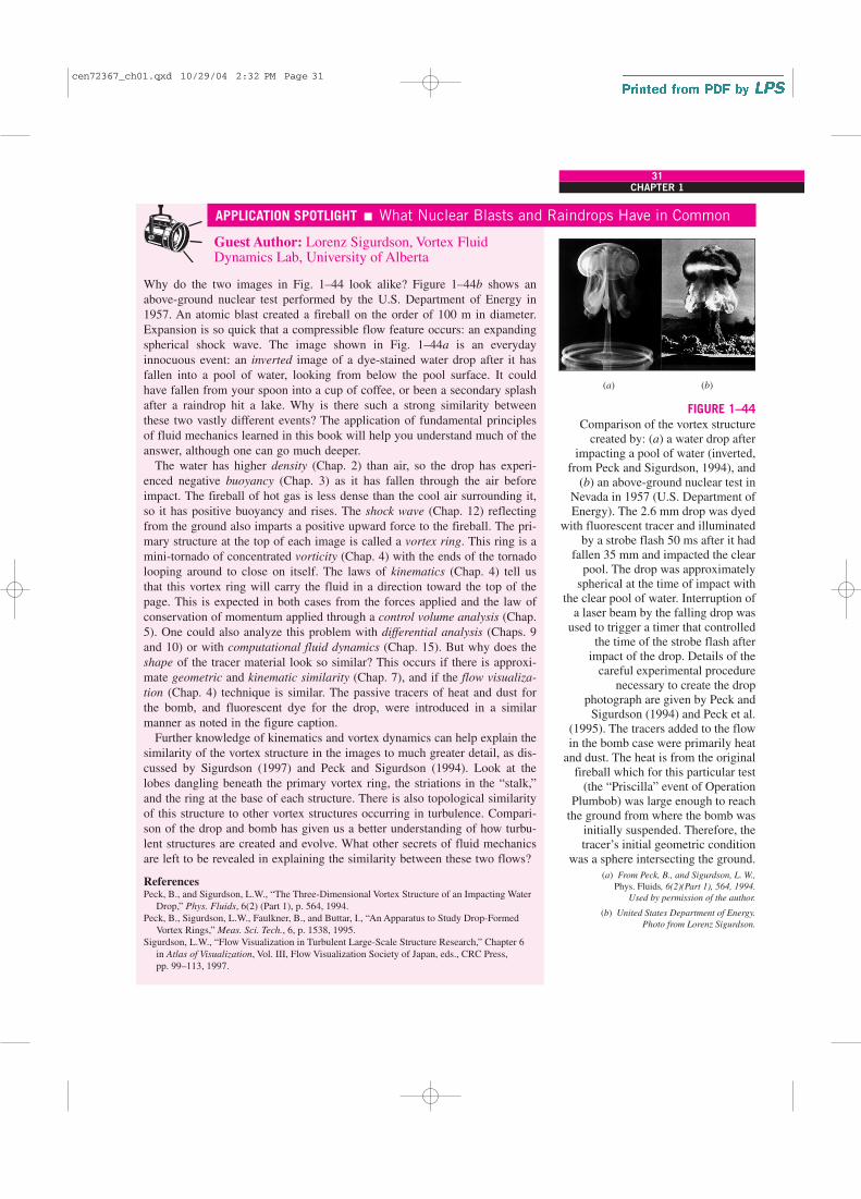
31CHAPTER 1

Guest Author: Lorenz Sigurdson, Vortex FluidDynamics Lab, University of Alberta

Why do the two images in Fig. 1–44 look alike? Figure 1–44b shows an

above-ground nuclear test performed by the U.S. Department of Energy in

1957. An atomic blast created a fireball on the order of 100 m in diameter.

Expansion is so quick that a compressible flow feature occurs: an expanding

spherical shock wave. The image shown in Fig. 1–44a is an everyday

innocuous event: an inverted image of a dye-stained water drop after it has

fallen into a pool of water, looking from below the pool surface. It could

have fallen from your spoon into a cup of coffee, or been a secondary splash

after a raindrop hit a lake. Why is there such a strong similarity between

these two vastly different events? The application of fundamental principles

of fluid mechanics learned in this book will help you understand much of the

answer, although one can go much deeper.

The water has higher density (Chap. 2) than air, so the drop has experi-

enced negative buoyancy (Chap. 3) as it has fallen through the air before

impact. The fireball of hot gas is less dense than the cool air surrounding it,

so it has positive buoyancy and rises. The shock wave (Chap. 12) reflecting

from the ground also imparts a positive upward force to the fireball. The pri-

mary structure at the top of each image is called a vortex ring. This ring is a

mini-tornado of concentrated vorticity (Chap. 4) with the ends of the tornado

looping around to close on itself. The laws of kinematics (Chap. 4) tell us

that this vortex ring will carry the fluid in a direction toward the top of the

page. This is expected in both cases from the forces applied and the law of

conservation of momentum applied through a control volume analysis (Chap.

5). One could also analyze this problem with differential analysis (Chaps. 9

and 10) or with computational fluid dynamics (Chap. 15). But why does the

shape of the tracer material look so similar? This occurs if there is approxi-

mate geometric and kinematic similarity (Chap. 7), and if the flow visualiza-

tion (Chap. 4) technique is similar. The passive tracers of heat and dust for

the bomb, and fluorescent dye for the drop, were introduced in a similar

manner as noted in the figure caption.

Further knowledge of kinematics and vortex dynamics can help explain the

similarity of the vortex structure in the images to much greater detail, as dis-

cussed by Sigurdson (1997) and Peck and Sigurdson (1994). Look at the

lobes dangling beneath the primary vortex ring, the striations in the “stalk,”

and the ring at the base of each structure. There is also topological similarity

of this structure to other vortex structures occurring in turbulence. Compari-

son of the drop and bomb has given us a better understanding of how turbu-

lent structures are created and evolve. What other secrets of fluid mechanics

are left to be revealed in explaining the similarity between these two flows?

ReferencesPeck, B., and Sigurdson, L.W., “The Three-Dimensional Vortex Structure of an Impacting Water

Drop,” Phys. Fluids, 6(2) (Part 1), p. 564, 1994.

Peck, B., Sigurdson, L.W., Faulkner, B., and Buttar, I., “An Apparatus to Study Drop-Formed

Vortex Rings,” Meas. Sci. Tech., 6, p. 1538, 1995.

Sigurdson, L.W., “Flow Visualization in Turbulent Large-Scale Structure Research,” Chapter 6

in Atlas of Visualization, Vol. III, Flow Visualization Society of Japan, eds., CRC Press,

pp. 99–113, 1997.

FIGURE 1–44

Comparison of the vortex structurecreated by: (a) a water drop after

impacting a pool of water (inverted,from Peck and Sigurdson, 1994), and

(b) an above-ground nuclear test inNevada in 1957 (U.S. Department ofEnergy). The 2.6 mm drop was dyed

with fluorescent tracer and illuminatedby a strobe flash 50 ms after it had

fallen 35 mm and impacted the clearpool. The drop was approximately

spherical at the time of impact withthe clear pool of water. Interruption of

a laser beam by the falling drop wasused to trigger a timer that controlled

the time of the strobe flash afterimpact of the drop. Details of the

careful experimental procedurenecessary to create the drop

photograph are given by Peck andSigurdson (1994) and Peck et al.

(1995). The tracers added to the flowin the bomb case were primarily heat

and dust. The heat is from the originalfireball which for this particular test

(the “Priscilla” event of OperationPlumbob) was large enough to reach

the ground from where the bomb wasinitially suspended. Therefore, thetracer’s initial geometric condition

was a sphere intersecting the ground.

(a) From Peck, B., and Sigurdson, L. W.,

Phys. Fluids, 6(2)(Part 1), 564, 1994.

Used by permission of the author.

(b) United States Department of Energy.

Photo from Lorenz Sigurdson.

(a) (b)

APPLICATION SPOTLIGHT � What Nuclear Blasts and Raindrops Have in Common

cen72367_ch01.qxd 10/29/04 2:32 PM

32FLUID MECHANICS

PROBLEMS*

Introduction, Classification, and System

1–1C Define internal, external, and open-channel flows.

1–2C Define incompressible flow and incompressible fluid.Must the flow of a compressible fluid necessarily be treatedas compressible?

1–3C What is the no-slip condition? What causes it?

1–4C What is forced flow? How does it differ from naturalflow? Is flow caused by winds forced or natural flow?

1–5C What is a boundary layer? What causes a boundarylayer to develop?

1–6C What is the difference between the classical and thestatistical approaches?

1–7C What is a steady-flow process?

1–8C Define stress, normal stress, shear stress, and pressure.

1–9C What are system, surroundings, and boundary?

1–10C When is a system a closed system, and when is it acontrol volume?

Mass, Force, and Units

1–11C What is the difference between pound-mass andpound-force?

1–12C What is the difference between kg-mass and kg-force?

1–13C What is the net force acting on a car cruising at aconstant velocity of 70 km/h (a) on a level road and (b) on anuphill road?

1–14 A 3-kg plastic tank that has a volume of 0.2 m3 isfilled with liquid water. Assuming the density of water is1000 kg/m3, determine the weight of the combined system.

1–15 Determine the mass and the weight of the air con-tained in a room whose dimensions are 6 m � 6 m � 8 m.Assume the density of the air is 1.16 kg/m3. Answers: 334.1

kg, 3277 N

1–16 At 45° latitude, the gravitational acceleration as afunction of elevation z above sea level is given by g � a � bz,

where a � 9.807 m/s2 and b � 3.32 � 10�6 s�2. Determinethe height above sea level where the weight of an object willdecrease by 1 percent. Answer: 29,539 m

1–17E A 150-lbm astronaut took his bathroom scale (aspring scale) and a beam scale (compares masses) to themoon where the local gravity is g � 5.48 ft/s2. Determinehow much he will weigh (a) on the spring scale and (b) onthe beam scale. Answers: (a) 25.5 lbf; (b) 150 lbf

1–18 The acceleration of high-speed aircraft is sometimesexpressed in g’s (in multiples of the standard acceleration ofgravity). Determine the net upward force, in N, that a 90-kgman would experience in an aircraft whose acceleration is 6 g’s.

1–19 A 5-kg rock is thrown upward with a force of150 N at a location where the local gravitational

acceleration is 9.79 m/s2. Determine the acceleration of therock, in m/s2.

1–20 Solve Prob. 1–19 using EES (or other) software.Print out the entire solution, including the

numerical results with proper units.

1–21 The value of the gravitational acceleration g decreaseswith elevation from 9.807 m/s2 at sea level to 9.767 m/s2 atan altitude of 13,000 m, where large passenger planes cruise.Determine the percent reduction in the weight of an airplanecruising at 13,000 m relative to its weight at sea level.

Modeling and Solving Engineering Problems

1–22C What is the difference between precision and accu-racy? Can a measurement be very precise but inaccurate?Explain.

1–23C What is the difference between the analytical andexperimental approach to engineering problems? Discuss theadvantages and disadvantages of each approach.

1–24C What is the importance of modeling in engineering?How are the mathematical models for engineering processesprepared?

1–25C When modeling an engineering process, how is theright choice made between a simple but crude and a complexbut accurate model? Is the complex model necessarily a bet-ter choice since it is more accurate?

1–26C How do the differential equations in the study of aphysical problem arise?

1–27C What is the value of the engineering software pack-ages in (a) engineering education and (b) engineering prac-tice?

1–28 Determine a positive real root of this equationusing EES:

2x 3� 10x 0.5

� 3x � �3

* Problems designated by a “C” are concept questions, and

students are encouraged to answer them all. Problems designated

by an “E” are in English units, and the SI users can ignore them.

Problems with the icon are solved using EES, and complete

solutions together with parametric studies are included on the

enclosed DVD. Problems with the icon are comprehensive in

nature and are intended to be solved with a computer, preferably

using the EES software that accompanies this text.

cen72367_ch01.qxd 10/29/04 2:32 PM

CHAPTER 1

33

1–29 Solve this system of two equations with twounknowns using EES:

1–30 Solve this system of three equations with threeunknowns using EES:

1–31 Solve this system of three equations with threeunknowns using EES:

Review Problems

1–32 The weight of bodies may change somewhat from onelocation to another as a result of the variation of the gravita-

x � y � z � 2

x � 3y 0.5� xz � �2

x 2y � z � 1

xy � 2z � 8

3x 2� 2y � z � 2

2x � y � z � 5

3xy � y � 3.5

x 3� y 2

� 7.75

tional acceleration g with elevation. Accounting for this vari-ation using the relation in Prob. 1–16, determine the weightof an 80-kg person at sea level (z � 0), in Denver (z � 1610m), and on the top of Mount Everest (z � 8848 m).

1–33 A man goes to a traditional market to buy a steak fordinner. He finds a 12-oz steak (1 lbm = 16 oz) for $3.15. Hethen goes to the adjacent international market and finds a320-g steak of identical quality for $2.80. Which steak is thebetter buy?

1–34 The reactive force developed by a jet engine to pushan airplane forward is called thrust, and the thrust developedby the engine of a Boeing 777 is about 85,000 lbf. Expressthis thrust in N and kgf.

Design and Essay Problem

1–35 Write an essay on the various mass- and volume-mea-surement devices used throughout history. Also, explain thedevelopment of the modern units for mass and volume.

33CHAPTER 1

cen72367_ch01.qxd 10/29/04 2:32 PM

cen72367_ch01.qxd 10/29/04 2:32 PM

INTRODUCTION AND BASIC CONCEPTS I - kau 1.pdf · INTRODUCTION AND BASIC CONCEPTS ... tory of the...

Documents

Transcript of INTRODUCTION AND BASIC CONCEPTS I - kau 1.pdf · INTRODUCTION AND BASIC CONCEPTS ... tory of the...