AN INVESTIGATION OF A FREE JET

: AT LOW REYNOLDS NUMBERS

wid orH 0>O fC (N

George C. Greene

X

U* • CM UO V) 9 «

t U

o — .M «*

•c 03 «oO (H ZH m ^t-t 13OT C5 •WSB >> -rlSB C/7 CHOD

,-485 O O

.rt S5 O

w o—.MS -H

vO 9 Om o aO» i-)VO T3

wi •< 0

«: H | infr< M f^im to •

t V ^^

^T^!& co Q55 1A

2^ So^ s:LU 0 SZ r-Ol

> 25 ^^C§ rau tei- P?<

tow

SB«a>

%»« e-i tn

A thesis presented

in .partial fulfillment of the requirements

for the degree of

MASTER OF, EKGDTESRllTG

Department of Mechanical EngineeringOld Dominion UniversityAugust 1973

Supervisory Committee

(Thesis Director)

https://ntrs.nasa.gov/search.jsp?R=19730021501 2018-06-02T19:39:34+00:00Z

ABSTRACT

This thesis presents a comparison of the measured and calculated

flow field properties of a nozzle of unusual design which vas used to

produce an incompressible, low Reynolds number jet. The "nozzle" is

essentially a porous metal plate vhich covers the end of a pipe.

Results are presented for nozzle Reynolds numbers from 50 to 1000

with velocities of 100 or 200 ft/sec. The nozzle produces a uniform

velocity profile at nozzle Reynolds numbers veil belov those at vhich

conventional contoured nozzles are completely filled with the boundary

layer. A Jet mixing analysis based on the boundary layer equations

accurately predicted the flow field over the entire range of Reynolds

numbers tested.

- ii -

TABLE OF CONTENTS

Page

ACKNOWLEDGEMENTS « iv

LIST OF FIGURES -AND TABLES v

LIST OF SYMBOLS vi

INTRODUCTION 1

APPARATUS 3

IMPACT TUBE VISCOUS CORRECTIONS. 5

TEST CONDITIONS AND PROCEDURE 10

JET FLOWFIELD ANALYSIS 13

DATA ACCURACY 17

RESULTS AND DISCUSSION 20

CONCLUSIONS 31*

- iii -

ACKNOWLEDGEMENTS

The author would like to express his appreciation to the

management of the Langley Research Center, NASA, for providing the

facilities and financial support for this thesis. The author would

also like to thank Dr. Donald F. Brink for his guidance, encouragement,

and assistance during the preparation of this thesis.

- iv -

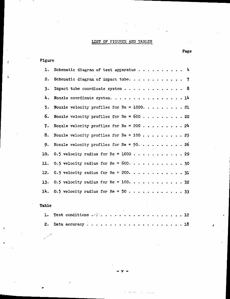
LIST OF FIGURES AND TABLES

Page

Figure

1. Schematic diagram of test apparatus U

2. Schematic diagram of impact tube 7

3- Impact tube coordinate systen 8

k. Nozzle coordinate system lU

5. Nozzle velocity profiles for Re = 1000 21

6. Nozzle velocity profiles for Re = 6"00 22

7- Nozzle velocity profiles for Re = 200 2k

8. Nozzle velocity profiles for Re = 100 25

9. Nozzle velocity profiles for Re = 50 26

10. 0.5 velocity radius for Re = 1000 29

11. 0.5 velocity radius for Re = 600 30

12. 0.5 velocity radius for Re = 200 31

13- 0.5 velocity radius for Re = 100 32

lU. 0.5 velocity radius for Re = 50 33

Table

1. Test conditions .--;• 12

2. Data accuracy 18

- v -

LIST OF SYMBOLS

K

M

P

R

Re

VT

u

v

Vmax

x,y,z

Y

P

Subscripts

e

0

T

specific heat at constant pressure

impact tube diameter

diffusion coefficient

impact tube viscous correction constant

thermal conductivity

Mach number

pressure

nozzle radius

•Reynolds number based on diameter

mass concentration of i'th gas

temperature

velocity in the x direction

velocity in the y direction

maximum nozzle velocity at a given value of x/R

nozzle coordinates

ratio of specific heats

density

coefficient of viscosity-*-"""

coordinates in the modifided Von Mises plane

conditions at y = °°

conditions at x = 0

stagnation conditions

- vi

- vii -

freestream conditions

impact tube conditions

INTRODUCTION

In the past decade several methods of measuring the temperature

of the earth's upper atmosphere have "been developed. In one of these

methods a small sounding rocket is used to carry an instrument package

and parachute aloft. The instrument package descends through the

atmosphere suspended "beneath the parachute and telemeters temperature

data to the ground. Due to the lov atmospheric density, the

temperature transducer has a lov degree of convective coupling to the

atmosphere. Solar radiation represents a significant portion of the

total heat transfer vhich results in degraded accuracy. In addition

the recovery factor nust "be knovn in order to correct for aerodynamic

heating. Therefore interpretation of the data requires calibration

on the ground vith flov conditions equivalent to those experienced

in the upper atmosphere.

In a typical calibration arrangement, the temperature transducer

is placed in a wind tunnel or jet of air to simulate the fall through

the atmosphere. The flow Mach number and Reynolds number are dupli-

cated to maintain the proper heat transfer characteristics.

However, for very low Reynolds numbers, which are required to

duplicate the conditions in the upper atmosphere, conventional wind

tunnel nozzles develop very thick boundary layers. This problem//

becomes serious at nozzle Reynolds numbers of about 1000 and gets

progressively worse until the entire nozzle is filled with the

boundary layer at Reynolds numbers of about 200 [l].

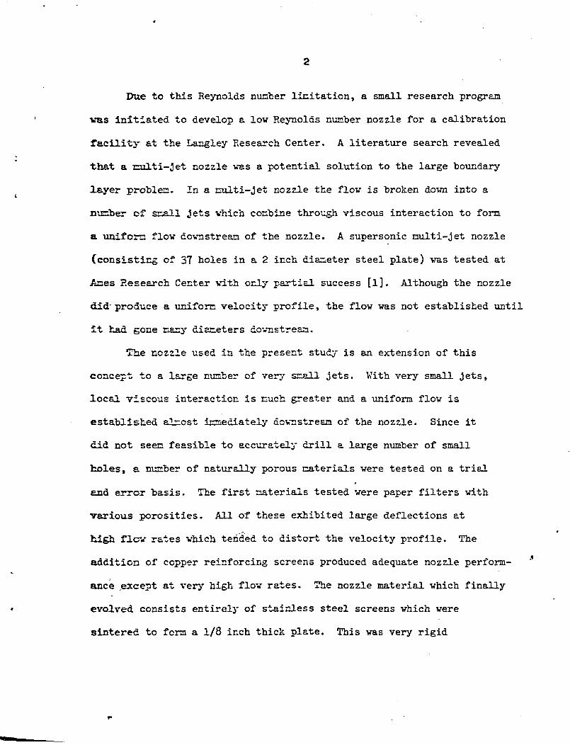
Due to this Reynolds number limitation, a small research program

vas initiated to develop a low Reynolds number nozzle for a calibration

facility at the Langley Research Center. A literature search revealed

•that a railti-jet nozzle vas a potential solution to the large "boundary

layer problem. In a multi-jet nozzle the flov is broken down into a

number of grv».n jets which combine through viscous interaction to form

a uniform flow downstream of the nozzle. A supersonic multi-jet nozzle

(consisting of 37 holes in a 2 inch diameter steel plate) was tested at

Ames Research Center with only partial success [l]. Although the nozzle

did'produce a uniform velocity profile, the flow was not established until

it had gone many diameters downstream.

The nozzle used in the present study is an extension of this

concept to a large number of very STB 11 jets. With very small jets,

local viscous interaction is much greater and a uniform flow is

established almost immediately downstream of the nozzle. Since it

did not seem feasible to accurately drill a large number of small

holes, a number of naturally porous materials were tested on a trial

and error basis. The first materials tested were paper filters with

various porosities. All of these exhibited large deflections at

high flow rates which tended to distort the velocity profile. The

addition of copper reinforcing screens produced adequate nozzle perform-

ance except at very high flow rates. The nozzle material which finally

evolved consists entirely of stainless steel screens which were

sintered to form a 1/8 inch thick plate. This was very rigid

and produced a reasonably uniform velocity profile over a vide range

of flovrates.

The purpose of this thesis is to describe the performancei

characteristics of this nozzle for nozzle Reynolds numbers between

50 and 1000 and to ccspare the nozzle flowfield data vith the calcu-

lated results of an incompressible boundary layer type analysis.

APPARATUS

Figure 1 shovs s. schematic diagram of the test apparatus used

in this investigation. The porous plate nozzle vas bolted to the end

of a 7-5/8 inch diameter nozzle pipe which extended through the wall

of a large (55 feet diameter) vacuum, chamber. The porous plate

nozzle vas made of 5 layers of stainless steel screen which were

sintered to form a rigid plate 1/8 inch thick. The innermost screen

had a mesh size of about 5 nicroinches. The outer screens were of a

larger nesh size for strength. The sintered screens are sold commer-

cially by the Eendix Corporation, Filter Division under the brand

name Poroplate.

Outside the vacuum chamber an air supply was passed through a

dryer, pressure regulator, vertical tube flowmeter, and manual control

valve into the nozzle pipe. The airstream stagnation temperature

vas measured inside the nozzle pipe using a shielded thermocouple.

Downstream from the nozzle the flow Mach number was determined from

measurements of the static pressure and the difference between the

total and static pressures using the one-dimensional isentropic flow

equations.

Control valve

Flovsieter

regulator•

Vacuum cylinder vail

•Nozzle pipe 7 5/8" diameter

Porous plate nozzle

22" —

— Impacttube

Surveydevice

.Figure 1.- Schematic diagram of test apparatus.

The total pressure was determined from impact tube measurements

after applying a viscous correction. This correction is described in

detail in the section entitled "Impact Tube Viscous Corrections." A

Baratron differential pressure transducer with a range zero to 10

torr was used to measure the difference between the impact tube

pressure and the static pressure. The static pressure throughout the

jet was assumed to be the same as the background gas pressure since

the flow was subsonic. The background pressure was measured at a

point near the nozzle using a Baratron absolute pressure transducer

with a range zero to 10 torr. Both pressure transducers were kept in

a controlled temperature environment to minimize temperature effects.

The flowfield surveys were made by moving the impact tube with

a two-dimensional survey device. The survey device was constructed

and aligned so that surveys could be made either axially along the

nozzle centerline or vertically along a nozzle radius. Calibrated

potentiometers were used to indicate the distance in each, survey

direction.

All position, pressure, and temperature data were recorded on a

Vidar digital data acquisition system. This system recorded at a

rate of 1*0 data channels'per second and produced either magnetic tape,

printed output or both.

y-''' IMPACT TUBE VISCOUS CORRECTIONS

In this study the flow Kach number was determined from the total

end static pressures using the isentropic flow equations. The total

pressure was obtained from impact tube measurements after applying

viscous corrections. The impact tube used in this study is shown

schematically in Figure 2. It was constructed to duplicate (as nearly

as possible) a probe described by Sherman [2]. In [2], several probes

vere calibrated to determine the magnitude of the errors resulting from

viscous flov about the probes at lov Reynolds numbers.

A discussion of impact tube errors at lov Reynolds numbers and

an analytical solution for certain types of probes is given by Schaaf

[3]« For a probe pointing into the gas stream, a boundary layer forms

at the stagnation point on the tip of the probe. Using the coordinate

system shown in Figure 3» the y-component of the Navier-Stokes

equations for inconpressible flow along the stagnation streamline can

be written in the following form

-s A*" O57 J/

This equation can be integrated through the boundary layer to give

i co oo 2, 9y y = 6 3y y = 0,

since the pressure and velocity at the outer edge of the boundary layer^x

are the sace as in the free stream. From the continuity equation and

flov symmetry about the stagnation streamline, it follows that

9v _ 8u 3w _ 3u

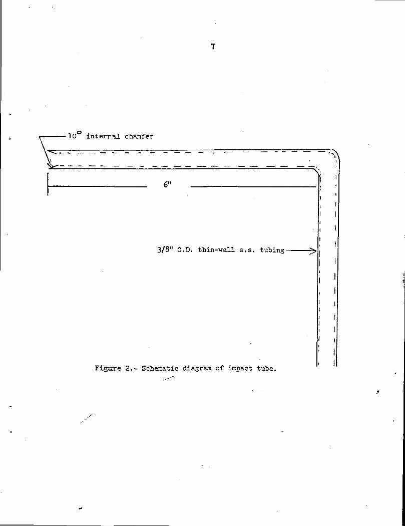
•10 internal chanfer

6"

3/8" O.D. thin-vall s.s. tubing'

Figure 2.- Schera.tic diagram of impact tube.

8

Boundary laver

^Stagnation point

Stagnation streamline

Figure 3.- Inpact tube coordinate system.

As a result of the boundary condition at the wall (T—) = 0,3xy = 0

equation (3) yields

Therefore equation (2) "becomes

U_, . « . /8u>

Proa a-c-crteE-tlel "Tl'ovssnai sis -ihe velocity gradient (T— ) .. canox y=o

be deterained ar lytically for simple shapes , such as a spherical

tipped probe [M- For a nore complicated geometry such as the open-

ended prcbe used in this study, (-r— ) .> can be approximated by

kA (u /D) vhere k is a constant which depends only on the probe

geometry. Th.e equation for inpact pressure then has the form

(5)

or

' kThus for large Reynolds numbers the correction term — is small andn

p. - p^ = pu^ /2. When the Reynolds number becomes very small,

p. - p^ becomes greater than

10

As previously mentioned the constant, k, depends on the probe

geometry, and must "be deternined experimentally. Since the probe used

in this study vas essentially a duplicate of one of the probes tested

"by Sherrian [2], a value of k • equal to 6, determined by fitting a

curve through the data in Figure 5 of [2], vas used.

Once the value of k is known, the flov velocity may be

calculated as follovs for incompressible flov:

R -P. -/ *

By rearranging end dividing by p/2, the above equation becomes

(„

free vhich one can solve for the velocity as

The values of p and }j in equation (9) are determined from the

static tenperature and pressure. Equation (9) therefore provides

the corrected velocity in terms of the measured parameters.

/TEST CONDITIONS AND PROCEDURE

Flovfield surveys vere made at nozzle Reynolds numbers of 50,

100, 200, 600, and 1000. Nominal flov velocities vere either 100

11

or 200 ft/sec. The resulting Mach numbers vere approximately 0.089

and 0.178, respectively, which vere sufficiently lov to insure essen~

tially incompressible flov conditions. The Reynolds number was varied

"by changing the density of the air. The flov conditions for each

Reynolds number are listed in Table 1.i

For testing at lov pressures a continuous flov capability is

highly desirable in order to allov sufficient run time to establish

stable flov conditions and make the required measurements. In the

present study continuous flov conditions vere maintained for all

nozzle flcvrs.te.5.

Before each test the static pressure transducer was checked

against a reference transducer to check for zero drift. The

differential pressure transducer which was used to measure the impact

tube pressure vas checked for zero drift when the chamber was at the

desired static pressure just prior to establishing the flov. The

desired flov conditions vere established based on the indicated dynamic

pressure frci-i the impact tube measurement with precomputed viscous

corrections. Preliminary surveys vere nade to establish the fact that

the jet vas axisymetric. Surveys vere then made from the jet center-

line outvard^along a radius at various positions along the jet axis.

Survey data vere recorded en the data acquisition system. After a

complete flovfield survey, the process vas repeated for the next/

Reynolds nuriher.

12

TABLE 1. TEST COIH)ITIONS

NozzleReynoldsKunber

50

100

200

600

1000

StaticP^CSSH-TC

x 103 ccKg

100

200

200

600

1000

DynanicPressurex 103 rrHg

0.55

1.09

U.U2

13.26

22.09

Pi -P.

x 10 imHg

1.86

2.U1

7.06

15.90

2U.T3

NominalVelocityft /sec

100

100

200

200

200

JET FLOVFIELD ANALYSIS

The Jet flovfield VH.S analyzed using the computer program

described "by Fox, Sinha and Weinberger [5]. The program has "been

adapted to the CDC 6COO series computer system and vas used vith only

superficial codifications.

Basically the progran solved the conpressible, axisymmetric

boundary layer equations in the Von Mises plane using an implicit

finite difference numerical technique. Thus the applicable equations

for the flov field -sjiefeche "in Figure J* are. as follows:

Conservation of riass

c PI//; -±y

do)

Conservation of ccsentua

Conservation of energy

(12)

, -- /, 213

Porousplatenozzle

- x

Nozzlecenterline

Figure .- Nozzle ccoridnate system.

15

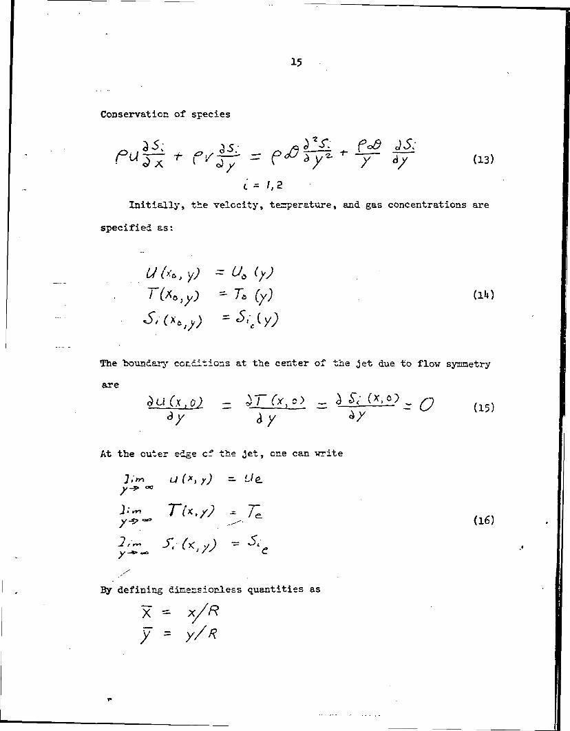
Conservation of species

* 57 - f^r " / 57c - /, 2

Initially, the velocity, tezperature , and gas concentrations are

specified as:

U(**>y) -

^ Te fy)

The "boundari' conditions at the center of the jet due to flow symmetry

are

*u Cx . ol - *T(x > - ajVJfi!' r /o ( .a/ iy

At the cuter edge cf the ,Jet, one can write

J*V> L/ f , y) — 'Je.y~& °"

x , 7;, -- (16)

y

By defining dinensionless quantities as

X - x/1?

7 =

uV

ef

16

=• u

/

(17)

tlie conservation equations can be solved in the modified Von Mises

plane vitich is defined for axisyr^netric flov by:

x

- >/ C- 4 J

c/X

(18)

r - (19)

rt should be noted that since the edge conditions were used to

normalize the velocities, the case of u = 0 cannot be solved.

Eovever, this is usually not a problen since u nay be made very

snail, and vas not zero in the actual experiment.

•ware*

DATA ACCURACY

An error estinate vas cade for each of the variables of interest

in this study. The errors in the measured quantities were determined

directly frcr: instrument characteristics. The errors in calculated

quantities vere "based on the errors of each measured quantity vhich

vas used in the calculation. An error summary is presented in Table 2.

The cass flov and total temperature accuracies are based on the

nanufacturers' specifications for each instrument. Since the nozzle

cass flov ra-ts *?£~s i ssd. nly for a .qualitative check of the average

nozzle velocity, -an additional nass flow calibration did not appear to

be Justified. !T>e +2°? total temperature error represents only 0.1*

percent of the absolute terrperature and is a relatively small error

source.

The error in both the static pressure and the difference between

the impact tube and static pressure is primarily due to instrument

zero drift. The static pressure transducer was located in a small

controlled environment chamber inside the large vacuum chamber. The

transducer vas not readily accessible for zero calibration since this

required physically purging the transducer to zero pressure. However,

a reference transducer vhich vas calibrated against a secondary

standard vas kept purped down to essentially zero pressure. Justfs

prior to each test, the static pressure vas measured using both

transducers and the reading of the static pressure transducer corrected

to the value indicated by the reference transducer. Zero check for

17

18

TABLE 2. DATA ACCURACY

Variable ErrorMagnitude

Cements

x,y

P

+.05 SCFM

+3xl ~3

+1x10

+.03 inch

1-Ianuf ecturer ' s spec.

J-Iacxifacturer ' s spec.

( Short tern accirracy

( Recalibrated for each test

Prinarily gear backlash

;*p.7 tc +3.1-2 Based on temperature and

to

r.e r.-.errors v&nd p-erf ectgas relatic-n.

Eased on .temperature error andSutberlszid ' scosity equation

Eased en pressure and temperatureerrors and 10? uncertainty inthe irnpact tube viscouscorrect icr. constant

Re to +11 Based on errors in p, v, and y

19

the differential pressure transducer vas relatively easy. This was

done Just before each test "before flov conditions vere established.

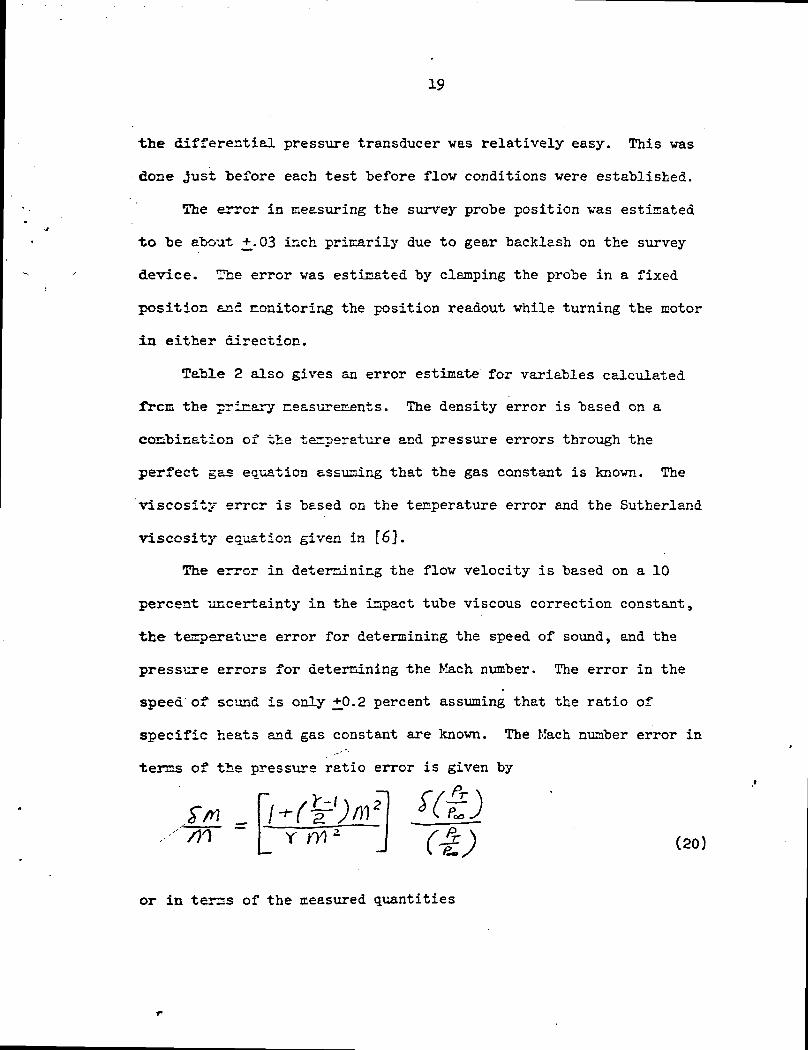
The error in measuring the survey probe position vas estimated

•to be about + 03 inch primarily due to gear backlash on the survey

device. The error vas estimated by clamping the probe in a fixed

position and monitoring the position readout vhile turning the motor

in either direction.

Table 2 also gives an error estimate for variables calculated

frcm the primary measurements. The density error is based on a

combination of the temperature and pressure errors through the

perfect gas equation assuming that the gas constant is knovn. The

viscosity error is based on the temperature error and the Sutherland

viscosity equation given in [6].

The error in determining the flov velocity is based on a 10

percent -uncertainty in the impact tube viscous correction constant,

the temperature error for determining the speed of sound, and the

pressure errors for determining the Mach number. The error in the

speed of sound is only +0.2 percent assuming that the ratio of

specific heats and gas constant are knovn. The Mach number error in

terms of the pressure ratio error is given by

/n •y

or in terns of the measured quantities

(-£) <2°)

20

(21)

The velocity error is then the s-on cf the Ksch number error end speed

of sound error.

The error in Reynolds number is sirrply the sun of the errors in

density, viscosity, and velocity. The error ic rLeasuring probe

dianeter is included in the uncertainty of the inpact tube viscous

correction constant.

RESULTS AXD DISCUSSION

Figure 5 Tvbsws the 'cav-si-opst-at x>f the jet -velocity profiles in

the dovnstrean direction for a nozzle Reynolds nurber of 1000.

Velocity profiles are shovn for three axial stations: x/R = 1, 2.5>

and 7- For each velocity profile, the ratic cf local velocity to

the Eaxinu-. jet velocity, v/v , vas plotted against the non-

dimensional radial coordinate, y/E. The synbcls represent the

measured data and the solid line represents the confuted results.

The neasurea and computed results are in good agreement, especially

in the nixing region except at x/H = 7- As can be seen a very

large potential core exists as far covnstreari as x/R = 7 which

vas the naxicun distance for vhich neasurenents vere taken. The cal-

culated results indicate that ihe potential core vould extend to about

x/R ="30.

Figure 6 shovs a set of velocity profiles for a nozzle Reynolds

nucber of 600. Again, v/v is plotted against y/R for x/R =t" y

1, 2.5> and 7-79- The agreement betveen calculated and neasured

F:

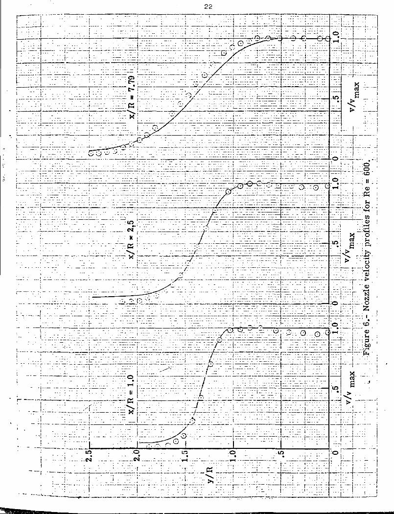
22

23

results is good except at 7-79- The potential core is still reasonably

large at x/R =7-79 and according to the analysis, it extended down-

stream to about x/R = 20.

Figure 7 shovs typical velocity profiles for a nozzle Reynolds

number of 200. v/v is plotted against y/R for x/R = 0.5, 2.5,m£-2£

and 6.0. The agreement between measured and calculated results is

again very good. The potential core extends dovnstream to about

x/R = 6. At x/R = 0.5 and 2.5j there is a reasonably large region of

uniform velocity. It should be noted that at Reynolds numbers of about

200, a conver.tic.cel ••eciiioizred nozzle vould be nearly filled with

boundary layer at the nozzle exit.

Figure 8 sbovs the calculated and measured flow field data for a

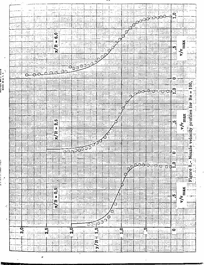
nozzle Reynolds number of ICO. v/v is plotted against y/R forTT'p.y

x/R = 0-5, 1.0, and 2.5. The potential core extends downstream just

slightly beyond x/H = 2.5. At x/R = 0.5 and 1.0 there still remains

a relatively large area of uniform flov.

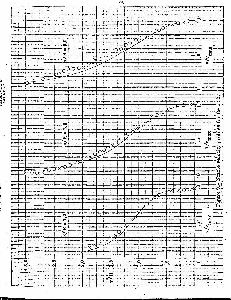
Figure 9 shovs the velocity profiles for a nozzle Reynolds number

of 50, the lovest Reynolds number at which flow surveys were nade.

v/v is again plotted versus y/R for x/R = 1.0, 2.5, and 5.0.max

The potential core extends dovnstream to only about x/R = 1.0. The

calculated results, vhich agree vith the data very well further

downstream, indicate that there is a large region of uniform flows'

Just dovnstream of the nozzle. For example, at x/R = 0.5. the

calculated results indicate that the potential core extends out

radially to y/R = 0 . 5 -

IS

•--(- I-- —T..

^_ _ ; , , _^, .. _„ . . . _ . . . . 1 ^^ _.__J

,27

As mentioned earlier, the agreement between the measured and

calculated results is very good with only a few exceptions. The

agreement would probably be even better if it were not for two prob-

lems in calculating the flow field. The first problem is with the

initial velocity profile which is used to start the flow field

calculations. It was assumed that at the nozzle exit the velocity

vas uniform across the entire nozzle. At the edge of the nozzle,

it vas assumed that the velocity made a step change to the value

associated with the background gas. However, the data indicate that

•the velocity was not quite uniform across the nozzle, especially at

the higher Reynolds numbers. These errors enter the calculations

and produce a large part of the discrepancies.

The other problem is in the value of velocity used for the

background gas. The computer program which was used for these

> calculations is designed to handle either the flow field of a jet

or the wake flow behind a body. However, wake flow calculations are

its primary function. In wake calculations, it is very logical to

nondimensionalize the velocity in the wake to the external flow

velocity, u . However, this precludes calculating the flow field

of a Jet flowing into a fluid at rest since u would be zero and

the nondimensional velocities would be infinite. This normally would

not be a problem since u may be made arbitrarily small, and, as Pai

[7] has shown, the solution is not overly sensitive to changes in u .

However, for very low nozzle Reynolds numbers there is an additional

problem. The numerical calculation step size is based on the Reynolds

number of the external flow. At low nozzle Reynolds numbers, small

values of u produce prohibitively long run times. In this

study, u was taken to be 5 percent of the jet velocity for all

calculations. This produced reasonable run times without introducing

; excessively large errors in the calculated velocity profiles.i| The primary effect of u is to change the Jet spreading rate.i • e

I This effect is shown in Figures 10 through lU. The 0.5 velocity

| radius (value of y/R at which v/v = 0.5) is plotted versus x/RI

i for Reynolds numbers of 1000, 600, 200, 100, and 50. The 0.5 velocityt

i radius is a measure of the jet width and its change in the downstream

I direction is a measure of the Jet spreading rate. These figures showt

that the experimentally determined spreading rate is greater than that!j -calculated using a value of u which is 5 percent of the Jet velocity.

j This is also what one would expect intuitively.

] At nozzle Reynolds numbers of 50 and 100, the nozzle velocity wasIj 100 ft/sec rather than 200 ft/sec which was used for all the otherII tests conditions. In order to determine if this change had any

j affect on the results, flow field calculations were made for both|I 100 ft/sec and 200 ft/sec velocities at the same nozzle Reynolds

: number. The nondimensional velocity profiles were identical which

i indicates that the mixing and spreading of an incompressible jet is1j a function of only the Reynolds number.

30

x z

3S

32

2 —

33

! :r:

•00-

it"

i ^rrf —

_zmnr~jiiiii r~T"~l —^— r- --T^_ ~'i"_'7.~Ti"".r^a-T I

CONCLUSIONS

1. The porous plate nozzle produced a reasonably uniform

velocity profile over a range of Reynolds numbers from 1000 down to

50. This contrasts with a conventional contoured nozzle which would

have a large boundary layer at a Reynolds number of 1000 and would be

completely filled with boundary layer at Reynolds numbers on the

order of 200.

2. A conventional, boundary layer type analysis was sufficient

to accurately calculate the jet flow field for nozzle Reynolds

numbers as low as 50.

3. The calculated mixing and spreading of an incompressible Jet

issuing into a medium at rest was a function of the Reynolds number

only. Calculations at the same nozzle Reynolds number but different

velocities produced essentially identical results.

R&JV.EKEHCES

1. Stalder, J. R., "The Use of Low-Density Wind Tunnels in Aerodynamic

Research", Rarefied Gas Dynamics, Vol. 3, Pergamon Press, 19 0,

pp. 1-20.

2. Sherman, F. S., "New Experiments on Impact-Pressure Interpretation

in Supersonic and Subsonic Air Streams", NACA TH 2995, 1953-

3. Schaaf, S. A., "The Pitot Probe in Low-Density Flow", AGARD Report

525» January 1966.

1*. Pao, Richard, H. F., Fluid Dynamics, Charles E. Merrill Books, Inc.

1967, p. 201.

5. Fox, H., Sinha, R., and Weinberger, L., "An Implicit Finite Dif-

—ference Solution for Jet and Wake Problems", Astronautica Acta,

Vol. 17, No. 3, 1972.•

6. "Equations, Tables, and Charts for Compressible Flow", NACA TR 1135,

1953.

7. Pal, Shih - I, Fluid Dynamics of Jets, D. Van Nostrand Co., Inc.

195U, P. 82.

35