Intro to Statistics for the Intro to Statistics for the Behavioral SciencesBehavioral Sciences

PSYC 1900PSYC 1900

Lecture 2: Basic Concepts Lecture 2: Basic Concepts andand

Data VisualizationData Visualization

Primary GoalPrimary Goal

Statistics

Why do we use statistics?Why do we use statistics?

Do statistics lie?Do statistics lie?

Adherence to Scientific Adherence to Scientific MethodMethod

Specific AssumptionsSpecific AssumptionsLong-Term ReplicabilityLong-Term Replicability

Is This Difference Is This Difference Meaningful?Meaningful?

Definition of TermsDefinition of Terms VariableVariable

A concept or entity of interest on which variability existsA concept or entity of interest on which variability exists Goal of behavioral science research is to explain why Goal of behavioral science research is to explain why

scores differscores differ

SampleSample Set of observations used in analysisSet of observations used in analysis Subset of the populationSubset of the population

PopulationPopulation Entire set of relevant observationsEntire set of relevant observations Findings with sample are used to generalize to Findings with sample are used to generalize to

populationpopulation

What is the Harvard Student Body?What is the Harvard Student Body?

Definitions ContinuedDefinitions Continued StatisticsStatistics

Numerical values summarizing sample dataNumerical values summarizing sample data Examples: mean, median, varianceExamples: mean, median, variance

ParametersParameters Numerical values summarizing population dataNumerical values summarizing population data We estimate population parameters based on We estimate population parameters based on

sample statisticssample statistics

Random SampleRandom Sample Sample in which each member of population Sample in which each member of population

has an equal chance of inclusion.has an equal chance of inclusion.

Descriptive vs. Inferential Descriptive vs. Inferential StatisticsStatistics

Distinct types for distinct purposesDistinct types for distinct purposes DescriptiveDescriptive

Purpose is to provide statistics that summarize Purpose is to provide statistics that summarize or capture nature of the sampleor capture nature of the sample

Mean is average scoreMean is average score Standard Deviation is measure of average dispersion Standard Deviation is measure of average dispersion

or deviation from the norm (i.e., how well the mean or deviation from the norm (i.e., how well the mean captures the score of the sample)captures the score of the sample)

InferentialInferential Purpose is to calculate probability that Purpose is to calculate probability that

differences in statistics across groups or levels differences in statistics across groups or levels of relationships among variables reflect the of relationships among variables reflect the operation of chance alone.operation of chance alone.

MeasurementMeasurement

In order to conduct analyses, we In order to conduct analyses, we have assign “values” or “codes” to have assign “values” or “codes” to observations.observations.

Different types of data require Different types of data require different types of scales.different types of scales. Scale types determine which analytic Scale types determine which analytic

procedures are appropriateprocedures are appropriate

Measurement ScalesMeasurement Scales There are two broad types containing There are two broad types containing

four subtypes.four subtypes. Qualitative: nominal scalesQualitative: nominal scales Quantitative: ordinal, interval, and ratio Quantitative: ordinal, interval, and ratio

scales.scales.

Nominal ScalesNominal Scales

Categorical in natureCategorical in nature No ordering is possibleNo ordering is possible

Examples: Religion, Ethnicity, GenderExamples: Religion, Ethnicity, Gender We can assign numerical codes, but they do not We can assign numerical codes, but they do not

represent any magnitude or ordering informationrepresent any magnitude or ordering information

Ordinal ScalesOrdinal Scales

Order is providedOrder is provided No information provided about magnitudes No information provided about magnitudes

of differences between points on the scaleof differences between points on the scale

Examples: RankingsExamples: Rankings We can again use numerical codes, but they do not We can again use numerical codes, but they do not

offer information on levels of difference or additivityoffer information on levels of difference or additivity

Interval ScalesInterval Scales

Order is providedOrder is provided Equivalence of differences between Equivalence of differences between

points is providedpoints is provided

Examples: Fahrenheit, Likert Scales (?)Examples: Fahrenheit, Likert Scales (?) Majority of statistical techniques we will cover Majority of statistical techniques we will cover

are designed for use with interval or ratio data.are designed for use with interval or ratio data.

Ratio ScalesRatio Scales

Order is providedOrder is provided Equivalence of differences between points Equivalence of differences between points

is providedis provided Scale has an absolute and meaningful zero Scale has an absolute and meaningful zero

point.point.

Examples: Kelvin, Salary, Hormone Levels Examples: Kelvin, Salary, Hormone Levels For ratio scaled data, we tend to use “raw” data For ratio scaled data, we tend to use “raw” data

descriptors. For interval, we often use “standardized” descriptors. For interval, we often use “standardized” descriptors (e.g., z-scores)descriptors (e.g., z-scores)

More DefinitionsMore Definitions Discrete VariablesDiscrete Variables

Take on smallish sets of possible valuesTake on smallish sets of possible values Continuous VariablesContinuous Variables

Variables that can take any valuesVariables that can take any values

Independent VariablesIndependent Variables Variables that are controlled by experimenter Variables that are controlled by experimenter

or designated as possible causal factorsor designated as possible causal factors Dependent VariablesDependent Variables

Variables being measured as data theorized to Variables being measured as data theorized to be caused by independent variablesbe caused by independent variables

Random SamplingRandom Sampling Used to ensure that composition of sample Used to ensure that composition of sample

“matches” composition of population“matches” composition of population

If sample deviates from population, generalizability is threatenedIf sample deviates from population, generalizability is threatened Randomization happens in many ways:Randomization happens in many ways:

Randomization programs, random number tablesRandomization programs, random number tables Note that Chance is lumpyNote that Chance is lumpy

Convenience samplesConvenience samples

Random AssignmentRandom Assignment

Used to ensure that composition of Used to ensure that composition of groups are equivalentgroups are equivalent

If groups deviate on relevant variables, validity of experiment is If groups deviate on relevant variables, validity of experiment is reducedreduced

Purpose of the control group is to “match” treatment group in every Purpose of the control group is to “match” treatment group in every way except experimental manipulation.way except experimental manipulation.

NotationNotation Sigma (Sigma () is the symbol for summation.) is the symbol for summation.

1,7,5,3

1 7 5 3 16i

i

X

X

Rules of summation.Rules of summation.

X Y X Y

CX C X

X C X NC

Sample DataSample DataDecade

(X) Family Size(Y)

X2

Y2

X – Y

XY

3 5.2 9 27.04 -2.2 15.6

4 4.8 16 23.04 -0.8 19.2

5 3.5 25 12.25 1.5 17.5

6 2.5 36 6.25 3.5 15.0

7 2.3 49 5.29 4.7 16.1

25 18.3 138 73.87 6.7 83.4

X 2X X Y

XY

22X X

Visualizing DataVisualizing Data

One of most useful things you can do One of most useful things you can do is display data visually.is display data visually.

As we’ll see, a picture is worth a As we’ll see, a picture is worth a thousand words when it comes to thousand words when it comes to checking assumptions of data.checking assumptions of data.

Frequency DistributionsFrequency Distributions

Presents data in a logical order that Presents data in a logical order that is easy to see.is easy to see.

Values of variable are plotted against Values of variable are plotted against their frequency of occurrence.their frequency of occurrence.

Data: 1,1,1,1,1,2,2,2,3Data: 1,1,1,1,1,2,2,2,3

Raw Data

0 1 2 3 4

Cou

nt

0

1

2

3

4

5

6

Problems with Frequency Problems with Frequency DistributionsDistributions

Sensitive to individual frequencies as Sensitive to individual frequencies as opposed to general patternsopposed to general patterns

With a highly variable scale, there With a highly variable scale, there may be very few indices of specific may be very few indices of specific valuesvalues

In such cases, a histogram provides a In such cases, a histogram provides a better description of the databetter description of the data

HistogramsHistograms

Graph in which bars represent frequencies Graph in which bars represent frequencies of observations within specific intervalsof observations within specific intervals

Each observed frequency

Binned into 6 intervals

(34.5 – 38.5;

38.5 – 42.5;

Etc.)

No true optimal number of intervals.

Ten is a good rule of thumb.

Stem and Leaf DisplaysStem and Leaf Displays

The benefits of stem and leaves is The benefits of stem and leaves is that they show both pattern of that they show both pattern of frequencies and actual individual frequencies and actual individual level data itself.level data itself.

As the name implies, the data are As the name implies, the data are separated into “stems” (i.e., leading separated into “stems” (i.e., leading digits) and “leaves” (i.e., following digits) and “leaves” (i.e., following digits marking each data point).digits marking each data point).

StemStem Vertical axis comprised of leading digitsVertical axis comprised of leading digits

Trailing DigitsTrailing Digits Digits to the right of the leading onesDigits to the right of the leading ones

LeavesLeaves Horizontal axis of trailingHorizontal axis of trailing

digitsdigitsStem-and-Leaf Plot Frequency Stem & Leaf 2.00 0 . 69 5.00 1 . 01222 5.00 1 . 67789 4.00 2 . 1223 2.00 2 . 57

Stem width: 10.00

6,9,10,11,12,12,12,

16,17,17,18,19,21,

22,22,23,25,27

Data

Stem-and-leaf of RxTime N = 300Leaf Unit = 1.0

7 3 6788999 27 4 00001112223333344444 62 4 55555566666666666777777777888899999 103 5 00000111111111111222222222233333333444444 150 5 55555556666666666777777788888888888899999999999 150 6 000000000000111111111112222222222222233333333334444444 96 6 555555556666666677777777777777889999999 57 7 0111122222222333444444 35 7 5566667788899 22 8 000112333 13 8 5678 9 9 044 6 9 558 3 10 44 1 10 1 11 1 11 1 12 1 12 5

The nature of the stems is determined by visual ease.

Here, there are two stems for each digit, broken at the midpoint.

Outlier

Height Stem & LeafHeight Stem & Leaf

Looking for Volunteers!!!

Modality & SkewnessModality & Skewness

ModalityModality Number of meaningful peaksNumber of meaningful peaks

Unimodal=1, Bimodal=2Unimodal=1, Bimodal=2

SkewnessSkewness Measure of the asymmetry of a Measure of the asymmetry of a

distributiondistribution Positive skew: tail to the rightPositive skew: tail to the right Negative skew: tail to the leftNegative skew: tail to the left

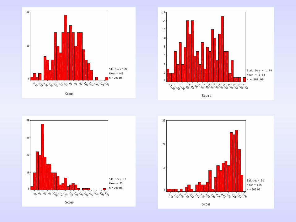
Score

2.832.43

2.031.63

1.23.83

.43.03

-.37-.77

-1.17-1.57

-1.98-2.38

-2.78

20

10

0

Std. Dev = 1.02

Mean = -.01

N = 200.00

Score

5.505.00

4.504.00

3.503.00

2.502.00

1.501.00

.500.00

-.50-1.00

-1.50-2.00

16

14

12

10

8

6

4

2

0

Std. Dev = 1.79

Mean = 1.54

N = 200.00

Score

4.394.07

3.753.44

3.122.80

2.492.17

1.851.54

1.22.90

.59.27

-.05

40

30

20

10

0

Std. Dev = .73

Mean = .96

N = 200.00

Score

5.895.57

5.254.94

4.624.30

3.993.67

3.353.04

2.722.40

2.091.77

1.45

30

20

10

0

Std. Dev = .91

Mean = 4.85

N = 200.00