Intraspecific Trait Variation and its Effects on Food Chains

Don DeAngelisUniversity of Miami

Coral Gables, Florida USA

Workshop on Nonlinear Equations in Population BiologyEast China Normal University, Shanghai, China

May 25-27, 2013

Intraspecific Variation1. Traits such as skill at foraging and investment in anti-

predator defense may vary among individuals within a species population.

2. Traits such as the choice of what sort of habitat to utilize can also vary among individuals of a population.

Here the effects of both types of variation are examined. This intraspecific variation has implications for both fitness strategies within a population and food web dynamics.

I. Intraspecific Variation in foraging ability, predator avoidance, and other mortality risk

Intraspecific variation within populations has been shown to be nearly ubiquitous in nature and to play an important role in community dynamics:

• D. I. Bolnick, P. Amarasekare, M. S. Araújo, R. Bürger, J. M. Levine, M. Novak, V. H. W. Rudolf, S. J. Schreiber, M. C. Urban, and D. A. Vasseur, Why intraspecific trait variation matters in community ecology, Trends Ecol. Evol,, 26:183-192 (2011).

• D. I. Bolnick. R. Svanbäck, J. A. Fordyce, L. H. Yang, J. M. Davis, C. D. Hulsey, and M. L. Forister, The ecology of individuals: incidence and implications of individual specialization. Amer. Natur., 161:1-28 (2003).

• M. Wolf, and F. J. Weissing, Animal personalities: consequences for ecology and evolution. Trends in Ecol. Evol., 27:452-461 (2012).

• How does this intraspecific variation relate to strategies for fitness of individuals in a population?

• Given the existence of subpopulations having distinct

sets of traits or strategies within a population, and that there is probably continuous switching of individuals between these subpopulations affect these dynamics?

Basic Questions

M

Predator

N1

Consumer 1

N2

Consumer 2

R

Resource

a2RN2 a1RN1

f2N2Mf1N1M

m12N1

m21N2

To investigate trait variation, we consider a tri-trophic chain of ‘resource R’, ‘consumer N’, and ‘predator M’

The consumer is assumed to have two phenotype subpopulations (with different strategies) and there is some switching back and forth between the two.

M

N1N2

R

a2RN2 a1RN1

f2N2Mf1N1M

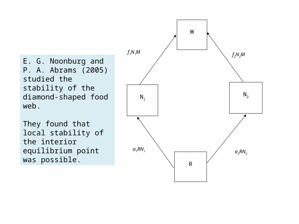
This chain resembles the ‘diamond-shaped’ chain that has been studied before; e.g.,

E. G. Noonburg and P. A. Abrams, Transient dynamics limit the effectiveness of keystone predation in bringing about coexistence, Amer. Natur. 165:322-335. (2005).

In this case the two consumers are different species, so there is no movement between the two consumer strategies.

22111 RNaRNaK

RrR

dt

dR

2211121111111 NmNmMNfNdRNba

dt

dN

2211122222222 NmNmMNfNdRNba

dt

dN

MdMNcfMNcfdt

dMm 2211

,

A simple set of equations for this system is as follows:

Parameters ai , di, and fi may differ between the two consumer phenotypes.

Resource

Consumer Phenotype 1

Consumer Phenotype 2

Predator

001 1211

1

111

1

11

**

,*,

* MNKba

d

a

rN

ba

dR

010 22

2

22212

2

22

**

,*

,* M

Kba

d

a

rNN

ba

dR

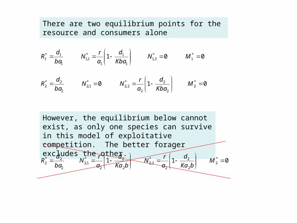
There are two equilibrium points for the resource and consumers alone

However, the equilibrium below cannot exist, as only one species can survive in this model of exploitative competition. The better forager excludes the other.

011 22

2

222

2

2

212

2

22

**

,*

,* M

bKa

d

a

rN

bKa

d

a

rN

ba

dR

1

1112

1

1323

113

1

13 01

f

d)darcf(

rcf

KbaMN

cf

dN

rcf

daKR m

**,

m*,

m*

1

2222

2

24

22414

2

24 01

f

d)darcf(

rcf

KbaM

cf

dNN

rcf

daKR m

*m*,

*,

m*

But at least one of the tri-trophic chains is assumed exist; i.e., the better forager is poorer at evading the predator.

0111 m*, dNcf

(1)

(2)

Assume that (1) exists; that is, that

This provides a path to the full system, if consumer 2 can invade; i.e., if

011 11

11122

1

1232232

)d

rcf

daKba)(f/f(d

rcf

daKbaMfdRba mm**

This means that the poorer forager can now invade, because the predator suppresses the better forager to some extent.

)fafa(b

dfdfR*

1221

21125

1

1

1221

2112

1

15 f

d

)fafa(b

dfdf

f

baM *

22112

211221122

2112

215 )fafa(Kb

)]dfdf()fafa(Kb[rf

)fafa(c

daN m*

,

22112

211221121

2112

125 )fafa(Kb

)]dfdf()fafa(Kb[rf

)fafa(c

daN m*

,

To obtain this solution we also make the assumption that the consumers are in an Ideal Free Distribution at equilibrium, so that m12N1* = m21N2*. This means that the individuals are distributed among the two strategies such that changing will not improve their fitness. There is still switching, but it is balanced.

We can find the interior equilibrium point.

M

N1N2

R

a2RN2 a1RN1

f2N2Mf1N1M

E. G. Noonburg and P. A. Abrams (2005) studied the stability of the diamond-shaped food web.

They found that local stability of the interior equilibrium point was possible.

However, they found that the system exhibits slowly damped extreme fluctuations, when the second consumer is introduced at small values.

This would likely lead to extinction of one or more of the species.

From Noonburg and Abrams , American Naturalist 2005

The question then is, what is the stability behavior of the analogous model for two consumer phenotypes in which continuous switching among the phenotypes occurs?

Analysis of the eigenvalues from the matrix

0

0

0

3231

2322112232

1312112131

32313

**

*,

*,

*,

*,

***

McfMcf

NfmmNba

NfmmNba

RaRaRK

r

shows that local stability is possible.

The eigenvalues can be further studied as a function of the movement rate m12, with m21 given by m12 N1*/N2*.

For m12 small, dynamics is dominated by complex conjugate eigenvalues with small negative real part.

As m12 is increased, the absolute value of the real part increases and then the solution bifurcates to two real eigenvalues.

R*

N2*

N1*For small m12 in the two consumer phenotype system, slowly damped large oscillations occur, as in Noonburg and Abrams (2005) model of a diamond-shaped web.

Simulations

R*

N1*

N2*

For larger m12, the transients damp more rapidly.

R*

N1*

N2*

For still larger m12 the long-term transient ceases to oscillate and damps monotonically

The remaining complex conjugate roots change little and continue to cause very rapidly damped oscillations, but these are not serious.

)fafa(b

dfdfR*

1221

21125

1

1

1221

2112

1

15 f

d

)fafa(b

dfdf

f

baM *

22112

211221122

2112

215 )fafa(Kb

)]dfdf()fafa(Kb[rf

)fafa(c

daN m*

,

22112

211221121

2112

125 )fafa(Kb

)]dfdf()fafa(Kb[rf

)fafa(c

daN m*

,

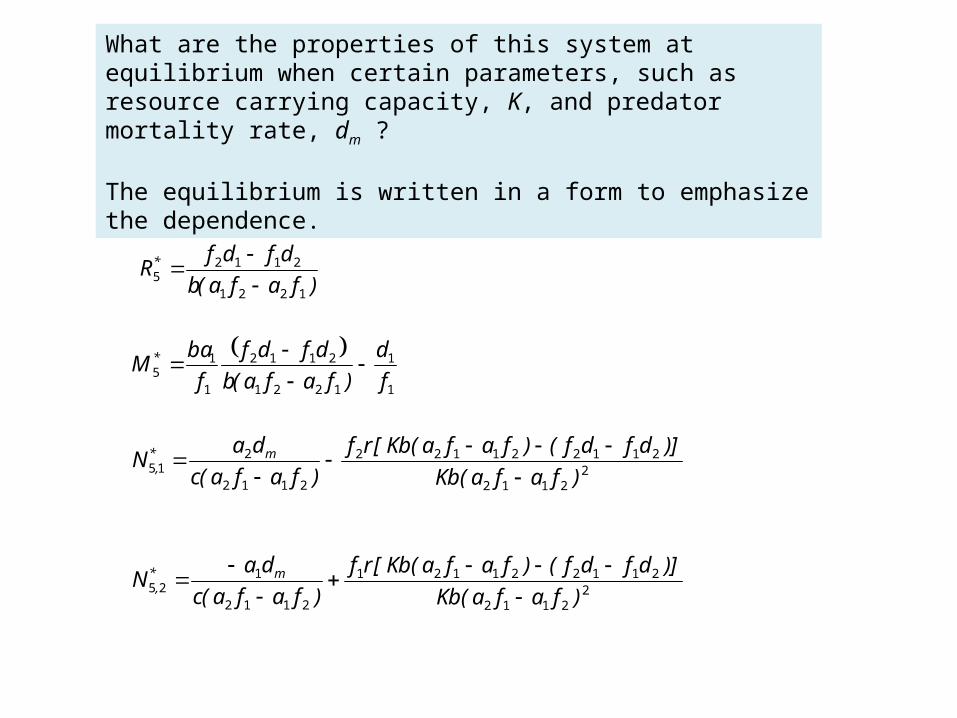
What are the properties of this system at equilibrium when certain parameters, such as resource carrying capacity, K, and predator mortality rate, dm ?

The equilibrium is written in a form to emphasize the dependence.

Let’s first review what happens in the single-consumer chain

aRNK

RrR

dt

dR

1

fNMdNbaRNdt

dN

MdcfNMdt

dMm

f

d)adrcf(

rcf

baKM

cf

dN

rcf

adKR m

*m*m*

21

,

with the equilibrium solution

Note that when K increases, R* increases and M* increases; N* does not change – alternating effects of bottom-up control.

When dm increases, M* decreases, N* increases, and R* decreases – cascading effects of top-down control.

Resource

Consumer

Predator

M*

R*

N1* + N2*

N2*

N1*

However, in the two consumer phenotype model, when K increases,

R* and M* remain the same and N1* + N2* either increases or decreases, the latter in this case.

R*

M*

N1* + N2*

N1*N 2*

In the case of two consumer phenotypes, when dm increases

R* and M* stay the same, and N1* + N2* either increases or decreases.

Therefore, there is a complete change in the bottom-up and top-down effects in a food chain when there are stably coexisting phenotypes of one consumer species.

Conclusions

Trophic cascades have been the object of intense interest by ecologists over the past few decades, because of both their scientific interest and management implications Several factors that affect the cascading of effects down the trophic chain have been noted.

Cascades in terrestrial food webs tend to be weaker than those of aquatic food webs, perhaps because of greater food web reticulation in those cases, including greater omnivory. The existence of diamond-shaped modules, a particular form of reticulation in many food webs, is another important factor. Therefore, the study of diamond-shaped webs is of special importance in understanding the propagation of cascades.

Noonburg and Abrams (2005) showed that the violent transient dynamics resulting from the indirect interactions of the two species might prevent the coexistence from lasting in practice. However, intraspecific diamond-shaped food webs, involving different phenotypes within a given consumer species, could be more plausible.

M

N1 N2 N3

R1 R2

The above results can be extended to some degree both to more complex models (e.g., to the left) and to other functional responses.

II. Intraspecific variation in habitat choice: with loss during movement

This is the second topic. Here we explore some of the consequences of two phenotypes of a consumer having traits such that one phenotype uses one habitat, with resources and predators, and the other uses another habitat, with a different set of resources and predator. Unlike the case above, we now assume there is energy loss or risk of mortality during movement between habitats (patches).

Extending ESS to systems where there is loss during movement

The Ideal Free Distribution (IFD) is commonly assumed for individuals of a species distributed across habitat patches. The IFD does not take into account that there can be losses in moving between habitat patches. However, because many populations exhibit more or less continuous population movement between patches, and travelling loss is a frequent factor, it is important to determine the effects of losses on expected population movement patterns and spatial distributions. It can be shown that, if movement among patches is assumed, an evolutionarily stable strategy (ESS) exists even when there are losses.

*Result of a NIMBioS workshop: Population and Community Ecology Consequences of Intraspecific Niche Variation (Bolnick et al. PIs)

DeAngelis, D. L., Gail S. K. Wolkowicz, Yuan Lou, Yuexin Jiang, Mark Novak, Richard Svanback, Marcio Araujo, YoungSeung Jo, and Erin Cleary. 2011. The effect of travel loss on evolutionary stable distributions of populations in space. The American Naturalist 178:15-29.

P1 P2

R1 R2

m12P1 (1-ε12)m12P1

(1-ε21) m21P2 m21P2

a1R1P1 a2R2P2

We considered bitrophic chains in which the consumer can move freely and continuously between two distinct patches with prey that are isolated in each patch, and has perfect knowledge of the patches…

Patch 1 Patch 2

Consumer, P

Resource, R

M1 M2

P1 P2

R1R2

m12P1 (1-ε12)m12P1

(1-ε21) m21P2 m21P2

f1P1M1 f2P2M2

a1R1P1 a2R2P2

… and we also considered tritrophic chains in which only the consumer can move freely between patches.

Patch 1 Patch 2

Predator, M

Consumer, P

Resource, R

The equations for the two systems are as follows…

Bitrophic

Tritrophic

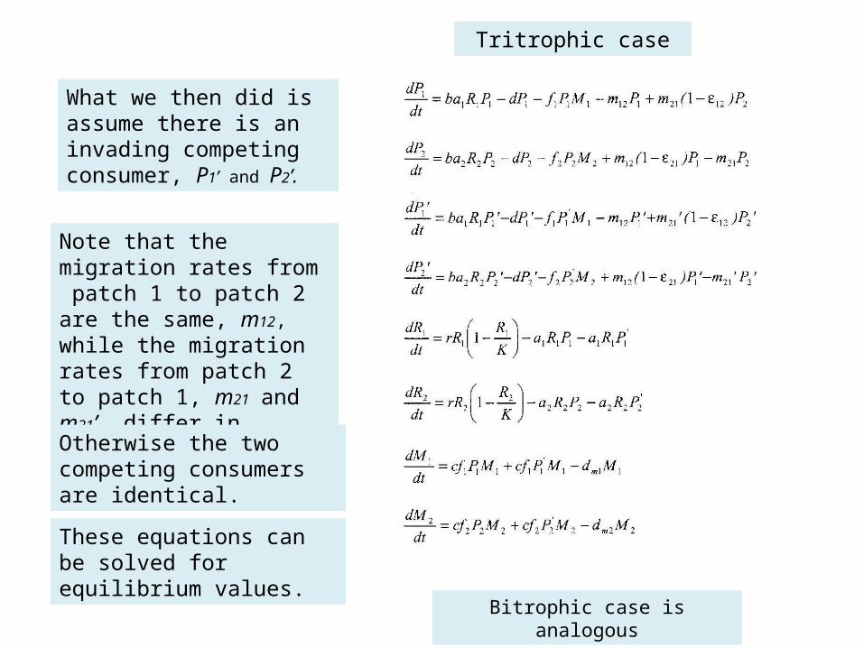
What we then did is assume there is an invading competing consumer, P1’ and

P2’.

Note that the migration rates from patch 1 to patch 2 are the same, m12, while the migration rates from patch 2 to patch 1, m21 and m21’, differ in general.

Tritrophic case

Bitrophic case is analogous

Otherwise the two competing consumers are identical.

These equations can be solved for equilibrium values.

We solved for the variables at equilibrium.

Equilibrium solution for tritrophic case

Note the bottom-up and top-down dependences are now the same as in the classical tritrophic food chain

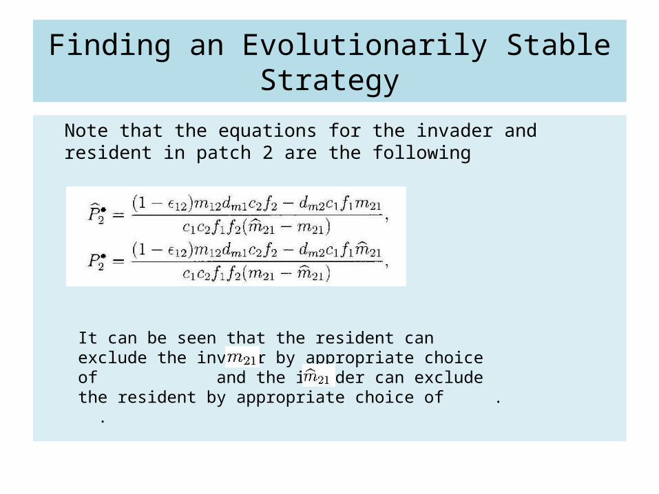
Finding an Evolutionarily Stable Strategy

Note that the equations for the invader and resident in patch 2 are the following

It can be seen that the resident can exclude the invader by appropriate choice of and the invader can exclude the resident by appropriate choice of . .

Equilibrium solution for bitrophic case

Similarly in this case, the resident or invader can choose a movement rate back to Patch 1 that excludes the other species.

So there is a value of m21 that the resident can choose such that it cannot be successfully invaded by any possible competitor; or, conversely, an invader using it that can replace any other strategy. Call it m21,opt.

Tritrophic case

Bitrophic case

This was shown to be an ESS. We can demonstrate numerically that a resident with any m21 ≠ m21,opt , can be successfully invaded by an invader that has m21’ = m21,opt (or that satisfies other conditions, see later). Suppose the two patches are entirely identical (all parameters are the same for the prey and consumers, in the bitrophic case). Suppose also that the resident has m12 = 0.01m21,opt.

Then let an invader with m12 and with m21’ = m21,opt appear.

Bitrophic model simulations confirm that an invader with m12‘ at the optimal value of m21,opt, starting from very small initial values, can exclude any alternative resident strategy.

ParametersP1’ and P2’P1 and P2

R1 and R2

Note that although the loss rate, ε21, for returning to patch 1 is huge, ε21 = 0.99, the strategy using the optimal return rate easily excludes the strategy using low return rate.

!

Invader P1’ and P2’

Resident P1 and P2

R1 and R2

There are some interesting properties of this result. One is the following. Suppose the two patches are entirely identical (all parameters are the same for the prey, predator, and consumers).

Suppose also that the resident has m12 = m21. Let an invader with m21’ = m21,opt appear with initially low numbers (0.000001).

Selection for spatial asymmetry: bitrophic case

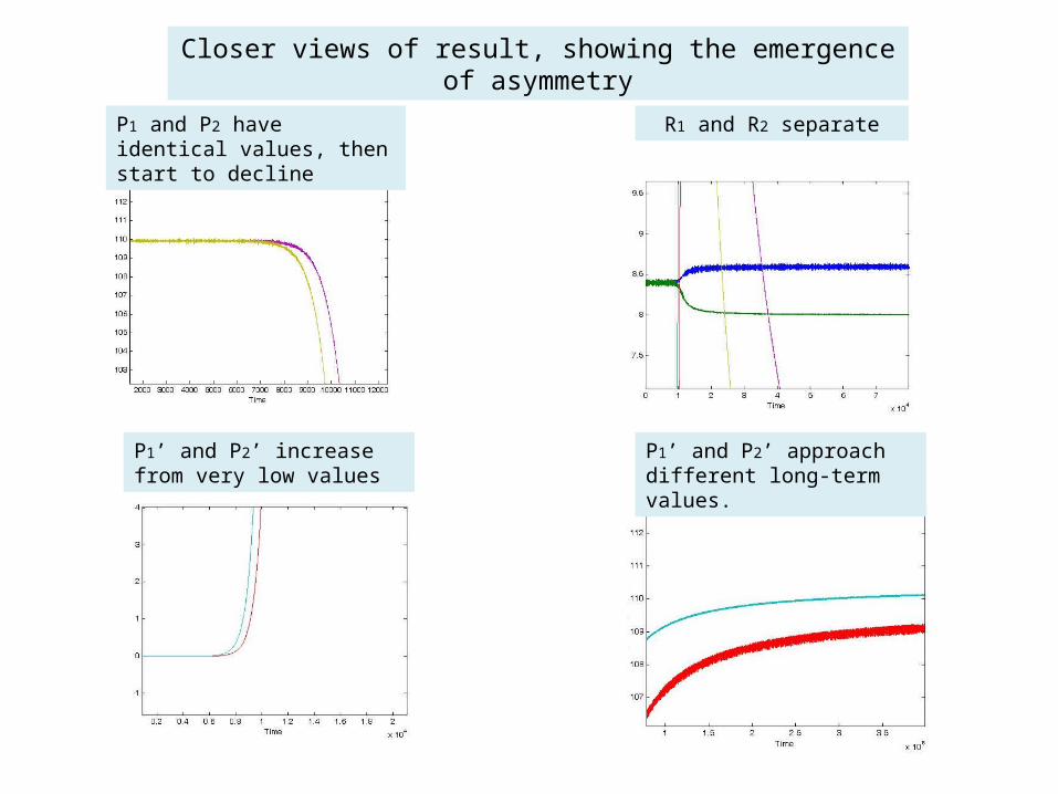
Closer views of result, showing the emergence of asymmetry

P1 and P2 have identical values, then start to decline

P1’ and P2’ increase from very low values

R1 and R2 separate

P1’ and P2’ approach different long-term values.

Result of asymmetry

This implies that the ESS for the distribution between identical patches is spatially asymmetric.

This asymmetry emerges both in the movement coefficients m12 and m21 and in the

values of R1* and R2

*, N1* and N2

* , and M1* and M2

*, even when the parameters of the

resources, consumers, and predators for the two subpopulations are precisely the same. This is strange, because it means that something also has to determine in which of the two subpopulation habitats the resource, consumer, and predator take the values R1

*, N1*, and M1

*, and in which these variables take the different values R2*, N2

*,

and M2*. This cannot be answered from the analysis above.

Natural selection creates asymmetry in an initially homogeneous system when there is loss in traveling.

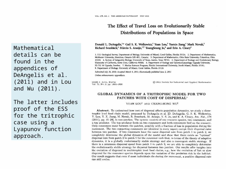
Mathematical details can be found in the appendices of DeAngelis et al. (2011) and in Lou and Wu (2011).

The latter includes proof of the ESS for the tritrophic case using a Lyapunov function approach.

Implications in nature: Stream drift

The passive downstream drift caused by one-directional flow of water is a common pattern and Müller (1954, 1982) hypothesized that insects compensate for downstream drift by a tendency for the adult forms to fly upstream to oviposit.

Implications in nature: Stream drift

Empirical studies have not conclusively supported the hypothesis that upstream movement of adults compensates for the loss, but have shown that substantial degree of compensation often occurs (Hershey et al. 1993 for mayflies)

Anholt (1995) proposed that such upstream movement may not be necessary, as density dependence occurs in the aquatic stages of many insects, and drift of individuals from a habitat patch may be compensated for by an increase in the survival rate of those remaining on the patch.

Kopp et al. (2001), nevertheless, showed through invasion analysis simulation, that even in such cases, upstream movement should be favored, because an insect genotype in which losses to drift from upstream to downstream patches are exactly compensated for by upstream movement will exclude any genotype for which this is not true.

Our results are more general than those of Kopp et al. (2001) and imply that if there are losses in either direction or both, the optimal level of compensation through upstream migration should be less than exact matching.

Further properties of ESS

21mopt,m21

Resident only

Invader only

Invader only

Resident only

Coexistence

Coexistence

21m̂

opt,m21

Resident’s migration rate from patch 2 to patch 1

Invader’s migration rate from patch 2 to patch 1

When neither resident nor invader has the optimal migration rate the results are more complex.

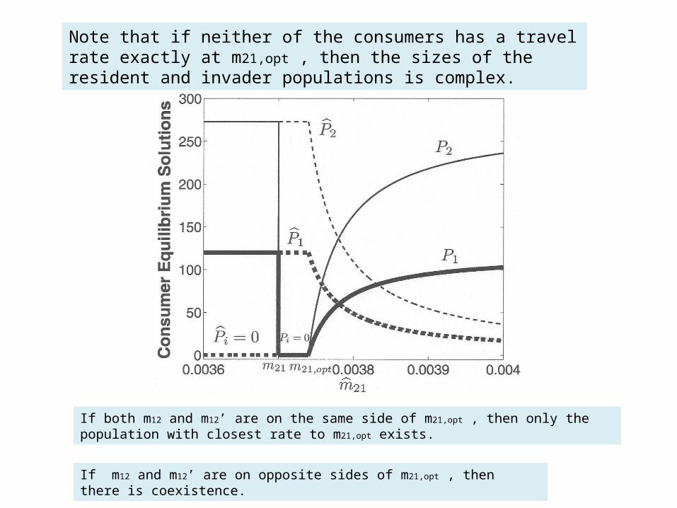
Note that if neither of the consumers has a travel rate exactly at m21,opt , then the sizes of the resident and invader populations is complex.

If both m12 and m12’ are on the same side of m21,opt , then only the population with closest rate to m21,opt exists.

If m12 and m12’ are on opposite sides of m21,opt , then there is coexistence.

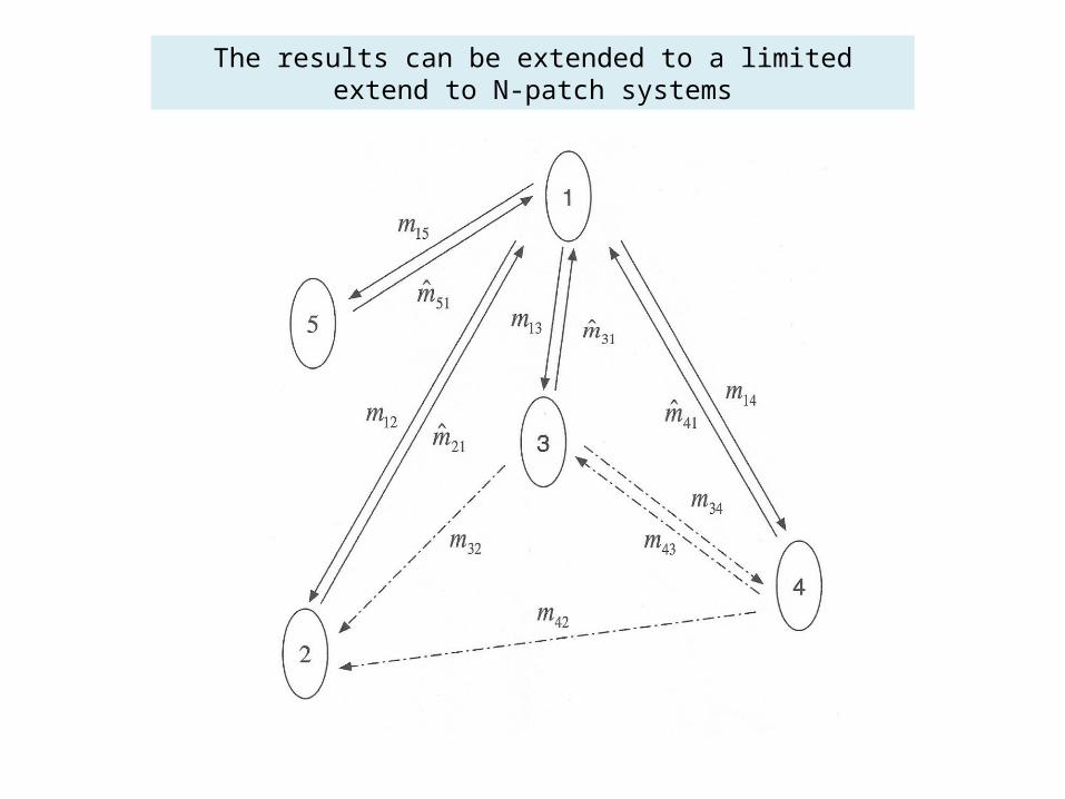
The results can be extended to a limited extend to N-patch systems

For a set of patches i = 1,N, the relevant equations for the tritrophic case can be written as

It seems very difficult to get solutions for the resident and invader, but a unique solution with the invader absent can be obtained.

An optimal movement rate can be obtained, but only under the assumption that all rates, when obtained, are positive.

From the above it seems there are a lot of open questions.

It should be again noted that we have made several assumptions

• It is assumed there is movement from at least one patch, which occurs from an ‘upstream’ patch.

• Populations are self-sustaining on every patch

• The different species or genotypes are identical in all respects accept in their return rates to the first patch.

The above is only a small part of theory involving traveling with loss. Much work relaxes the assumption of perfect knowledge.