P u b l ic I n t e re s t E n e r g y Re s e a r c h ( P I E R) P ro g r a m

F I N A L P R OJ E C T R E P O R T – R E V I E W DR A F T

Intra-hour solar power forecasting at util ity-scale power plants in the Los Angeles basin

2012

CEC-

Prepared for: California Energy Commission

Prepared by: Jan Kleissl, University of California, San Diego

Prepared by: Primary Author(s): Oytun Babacan, Guang Wang, Handa Yang, Jan Kleissl (corresponding author) Center for Renewable Resources and Integration, Department of Mechanical and Aerospace Engineering, University of California, San Diego. 9500 Gilman Dr., La Jolla, CA, 92093, +1 858 534 8087 Contract Number: 500-10-060 Prepared for: California Energy Commission Gail Wiggett Contract Manager

Prab Sethi Project Manager

XXXX XXXXXX Office Manager Name of Office Goes Here

XXXX XXXXXX Deputy Director Division Name Goes Here

Melissa Jones

Executive Director

DISCLAIMER

This report was prepared as the result of work sponsored by the California Energy Commission. It does not necessarily represent the views of the Energy Commission, its employees or the State of California. The Energy Commission, the State of California, its employees, contractors and subcontractors make no warrant, express or implied, and assume no legal liability for the information in this report; nor does any party represent that the uses of this information will not infringe upon privately owned rights. This report has not been approved or disapproved by the California Energy Commission nor has the California Energy Commission passed upon the accuracy or adequacy of the information in this report.

i

ACKNOWLEDGEMENTS

We would like to thank Southern California Edison (SCE) for supporting the project through hosting the sky imagers, providing access to the sites, providing data, and . In specific we would like to thank Sunil Shah, George Rodriguez, Theodore Luckham, Charles Lawless, Jermaine Woodall, Randall Lins, Darrell Holmes, Jerry Isaac, and Jack Peterson. Special thanks to ProLogis for providing building access and installation sites.

ii

PREFACE

The California Energy Commission Public Interest Energy Research (PIER) Program supports public interest energy research and development that will help improve the quality of life in California by bringing environmentally safe, affordable, and reliable energy services and products to the marketplace.

The PIER Program conducts public interest research, development, and demonstration (RD&D) projects to benefit California.

The PIER Program strives to conduct the most promising public interest energy research by partnering with RD&D entities, including individuals, businesses, utilities, and public or private research institutions.

PIER funding efforts are focused on the following RD&D program areas:

Buildings End-Use Energy Efficiency

Energy Innovations Small Grants

Energy-Related Environmental Research

Energy Systems Integration

Environmentally Preferred Advanced Generation

Industrial/Agricultural/Water End-Use Energy Efficiency

Renewable Energy Technologies

Transportation

Validation of the National Solar Radiation Database in California is the final report for the California Solar Energy Collaborative project (contract number 500-08-027) conducted by the University of California, San Diego. The information from this project contributes to PIER’s Renewable Energy Technologies Program.

For more information about the PIER Program, please visit the Energy Commission’s website at www.energy.ca.gov/research/ or contact the Energy Commission at 916-654-4878.

iii

ABSTRACT

For the first time, the forecast performance of the newly developed UCSD sky imager (USI) has been analyzed. Sky imagers were deployed for a year at a distribution feeder with four utility-scale warehouse rooftop solar power plants owned by Southern California Edison (SCE). Sky imager data and power output were available every 30 seconds. The largest 1 min ramps in power output were 46% of DC capacity for the smallest 1.7 MW plant, while the largest plant (5 MW) only showed ramps up to 25% of PV capacity.

Zero to fifteen minute power output forecasts for each of the four rooftop power plants were investigated over two months and two days were analyzed in greater depth. The difficulty of accurate cloud detection in the solar region causes sky imager forecast errors to be larger for 5 minute horizons. Forecast skill relative to persistence forecasts improves for longer horizons. Specific examples of promising ramp forecast skills were presented, but inaccuracies in cloud height limit ramp forecast accuracy.

USI forecast performance is also analyzed against a 1 minute resolution satellite forecast. The forecast errors are comparable with slight advantages for the USI.

Please use the following citation for this report:

Oytun Babacan, Guang Wang, Handa Yang, Jan Kleissl, Intra-hour solar power forecasting at utility scale power plants in the Los Angeles basin. CEC Report 500-10-060.

iv

TABLE OF CONTENTS

Acknowledgements ................................................................................................................................... i

ABSTRACT .............................................................................................................................................. iii

TABLE OF CONTENTS ......................................................................................................................... iv

EXECUTIVE SUMMARY ........................................................................................................................ 1

CHAPTER 1: INTRODUCTION ............................................................................................................ 4

CHAPTER 2: EXPERIMENTAL SETUP AND DATA ....................................................................... 6

2.1 Hardware Overview and Experimental Setup ............................................................................ 6

2.2 Data Availability .............................................................................................................................. 8

2.3 Data Selection for Further Analysis ............................................................................................... 8

CHAPTER 3: FORECAST PROCEDURES ........................................................................................... 9

3.1 Sky Imager Forecast Procedure ...................................................................................................... 9

3.1.1. Geometric calibration and image pre-processing ................................................................ 9

3.1.2. Detecting clouds ..................................................................................................................... 10

3.1.3. Cloud height, cloud map, and cloud velocity .................................................................... 11

3.1.4. Forecast site: domain and footprint ..................................................................................... 12

3.1.5. Cloud transmissivity ............................................................................................................. 12

3.1.6. Merge: cloud map advection, shadow map, and irradiance forecast ............................. 13

3.2 Error Metrics ................................................................................................................................... 13

3.2.1. Cloud map matching metrics ............................................................................................... 13

3.2.2. Aggregate error metrics ........................................................................................................ 14

3.3 Ramp Events ................................................................................................................................... 15

3.3.1. Ramp Event Detection ........................................................................................................... 15

3.3.2. Ramp Event Matching ........................................................................................................... 16

3.3.3. Ramp event forecast performance ....................................................................................... 16

CHAPTER 4: SKY IMAGER FORECAST RESULTS ....................................................................... 17

4.1 Case Studies .................................................................................................................................... 17

4.2. Aggregate results .......................................................................................................................... 22

4.3. Ramp rate distribution ................................................................................................................. 25

4.4. Ramp event detection ................................................................................................................... 26

v

4.5. Forecast improvements through cloud height correction ....................................................... 29

CHAPTER 5: SATELLITE FORECAST PERFORMANCE .............................................................. 31

5.1 Satellite Data Overview ................................................................................................................. 31

5.2 Satellite data selection for analysis .............................................................................................. 31

5.3 Method for analyzing satellite forecast performance ............................................................... 32

5.4 Satellite forecast performance compared to USI forecast ......................................................... 33

CHAPTER 6. CONCLUSIONS ............................................................................................................. 35

vi

1

EXECUTIVE SUMMARY

For the first time, the forecast performance of the newly developed UCSD sky imager (USI) has been analyzed. Sky imagers were deployed for over a year at a distribution feeder with four utility-scale warehouse rooftop solar photovoltaic (PV) power plants owned by Southern California Edison (SCE, Fig. ES-1). Sky imager data and power output were available every 30 seconds. The largest 1 min ramps in power output were 46% of DC capacity for the smallest 1.7 MW plant, while the largest 5 MW plant only showed ramps up to 25% of PV capacity.

Figure ES-1a: Photograph of sky imager as installed near Redlands, California.

Figure ES-1b: Sample sky image.

Zero to fifteen minute power output forecasts for each of the four power plants were analyzed over two months. After overcast and clear days were excluded, 17 days remained and average cloud properties on those days are shown in in Table ES-1. Cloud height averaged 2,400 m which is typical for continental sites and cloud speeds averaged 4.6 m s-1. Figure ES-2 shows an example of a sky imager nowcast, where sky imager cloud maps are projected in real-time onto the power plants. For this and a few other selected days the ramps detected by the sky imager match observed ramps very well and the sky imager forecast outperformed a smart persistence forecast. However, this is generally only the case for 5 out of the 17 days.

In principal, sky imagers have a unique ability to provide accurate forecasts of timing of ramps at utility scale power plants, since the temporal and spatial resolution of other forecast methods is inadequate. However, the present analysis shows that sky imager ramp forecasts were insufficient. Inaccurate cloud detection in the solar region and inaccurate cloud height specification likely limit ramp forecast accuracy. Further research is required to obtain accurate ramp forecasts from sky imagers for applications such as ramp smoothing.

2

Figure ES-2: Six hour period of USI Power nowcast (0 min forecast) for the power plant SPVP011 on April 16th, 2013. Y-axis labels were removed for confidentiality reasons.

Several other analyses point to the utility of sky imager forecast if forecast accuracy can be improved. The field-of-view was large enough to cover all the plants out to a 10 min horizon 93% of the time and even at a 15 min forecast horizon 85% coverage was observed (Table ES-1). Furthermore, the cloud-advection-versus-persistence (cap) error indicates that cloud advection was 22% superior to persistence at a 30 second forecast horizon, but only a 3% improvement existed at a 5 min forecast horizon.

Table ES-1: Average cloud conditions and cloud-advection-versus-persistence (cap) error for March and April 2013 for forecast horizons of 30 sec and 5 min. A cap error below 100% indicates that cloud advection outperformed persistence and confirms the potential of the sky imager forecast approach. FOV: Field of View. CBH: Cloud base height.

Avg % of plants in FOV

Avg. cloud fraction (%)

Avg. cloud speed (m/s)

Avg. CBH (m)

30 s 5 min 0 5 10 15 min

77.9 97.2 100 98 93 85 49.2 4.60 2355

USI forecast performance was also analyzed against forecasts derived from satellite imagery. The forecast errors are comparable with slight advantages for the USI (Table ES-2).

Table ES-2: USI and satellite aggregate power output error metrics by forecast horizon. A positive forecast skill (FS) indicates that the USI forecast outperforms the satellite forecast.

3

rMAE [%] rMAEs [%] FS [%]

Forecast Horizon [min] 0 5 10 15 5 10 15 5 10 15

rMAE [%] 18.0 18.9 17.6 24.0 17.8 19.1 23.4 2 12 8

4

CHAPTER 1: INTRODUCTION

Solar power presents a significant challenge because of high variability and uncertainty compared to conventional energy generation like natural gas or coal, while at the same time it is subject to environmental factors which are not controllable. SCE has installed over 30,000 PV systems on its distribution grid. The projected capacity for California-wide customer-installed PV systems is projected to be 3.2 GW in 2016. Variability in solar irradiance makes regulating and maintaining power both challenging and costly, as the uncertainty requires larger regulation and spinning reserve capacities to meet ancillary service requirements. Reduction in the uncertainty of solar power by solar forecasting methods can not only reduce the more expensive operating costs of ancillary services, but also allow energy traders to make more reliable bids in the wholesale energy market.

Of particular interest to the energy industry are sudden changes in irradiance, termed "ramp events"1, as ramp events in turn require ancillary services to ramp up or down to meet the change in electrical supply and maintain power quality. Cloud cover can result in such ramp events causing reductions in output by 50 to 80% within the time period it takes a large cloud to cover an array (typically on the order of 10 seconds). Short-term irradiance fluctuations can cause voltage fluctuations that can trigger automated line equipment (e.g. tap changers) on distribution feeders leading to larger maintenance costs for utilities. Given constant load, counteracting such fluctuations would require dynamic inverter VAR control or a secondary power source (e.g. energy storage) that could ramp up or down at high frequencies to provide load following services. Such ancillary services are costly to operate, so reducing short-term variation is essential. Longer scale variations caused by cloud groups or weather fronts are also problematic as they lead to a large consistent reduction in power generation over a large area. These long-term fluctuations are easier to forecast and can be mitigated by slower ramping (but larger) supplementary power sources, but the ramping and scheduling of power plants also adds costs to the operation of the electric grid. Grid operators are often concerned with worst-case scenarios, and it is important to understand the behavior of PV power output fluctuations over various timescales.

Therefore, solar forecasting plays a critical role in the integration of utility scale renewable energy (USRE). Accurate forecasts would allow load-following generation that is required to counteract ramps from USRE to be scheduled in the lower cost day-ahead market. Recent integration studies by National Renewable Energy Laboratory (NREL) and General Electric (GE) using 2020 renewable integration scenarios have shown economic values of renewable forecasting of $5 billion/year under 2020 USRE scenarios for the Western Electricity Coordinating Council (WECC) alone. With the advance of smart grid efforts the once autonomous operation of distribution system will also benefit from solar forecasting and solar resource variability analysis.

1 Pfister, G., McKenzie, R. L., Liley, J. B., Thomas, A., Forgan, B. W., Long, C. N., October 2003. Cloud coverage based on all-sky imaging and its impact on surface solar irradiance. Journal of Applied Meteorology and Climatology 42 (10), 1421 - 1434.

5

Our research addresses the need to accurately forecast the output from solar PV using sky imagery and determine the maximum amount of variability or ramp rate of solar output. We developed and validated our solar forecasting model with generation data from SCE USRE systems. In addition, statistical analysis of power output data yields the maximum amount of output variability in the form of ramp up/down rates.

Deterministic measurement-based forecasting typically involves measurements obtained from satellites or ground-based sky imagers. However, deterministic forecasting using sky imagers is still in its infancy, and approaches thus far include intra-hour DNI2, solar irradiance3 and real AC power forecasting for 48 MW of photovoltaics4 using a Total Sky Imager (TSI) produced by Yankee Environmental Systems.

This report presents an in-depth analysis of short-term solar irradiance forecasts generated using a whole sky imager developed at UC San Diego (UCSD Sky Imager or USI) at the SCE inland empire (Section 2). The USI forecast procedure will be presented (Section 3.1), validation metrics will be defined (Section 3.2) and ramp events analysis will be explained (Section 3.3). Following, the performance of the system will be analyzed by validating solar irradiance forecasts against two months (March and April 2013) of historical GHI data collected by four power plants. Due to the large validation set, results are generally presented in tables by averaging over each day, with particularly interesting days examined in greater detail.

2 Marquez, R., Coimbra, C. F. M., May 2013a. Intra-hour DNI forecasting based on cloud tracking image analysis. Solar Energy 91, 327 - 336.

3 Chow, C. W., Urquhart, B., Lave, M., Dominguez, A., Kleissl, J., Shields, J., Washom, B., 2011. Intra-hour forecasting with a total sky imager at the UC San Diego solar energy testbed. Solar Energy 85, 2881 - 2893.

4 Urquhart, B., Ghonima, M., Nguyen, D., Kurtz, B., Chow, C. W., Kleissl, J., 2013. Sky imaging systems for short-term solar forecasting, Jan Kleissl (Editor): Solar Energy Forecasting and Resource Assessment, Elsevier.

6

CHAPTER 2: EXPERIMENTAL SETUP AND DATA

2.1 Hardware Overview and Experimental Setup

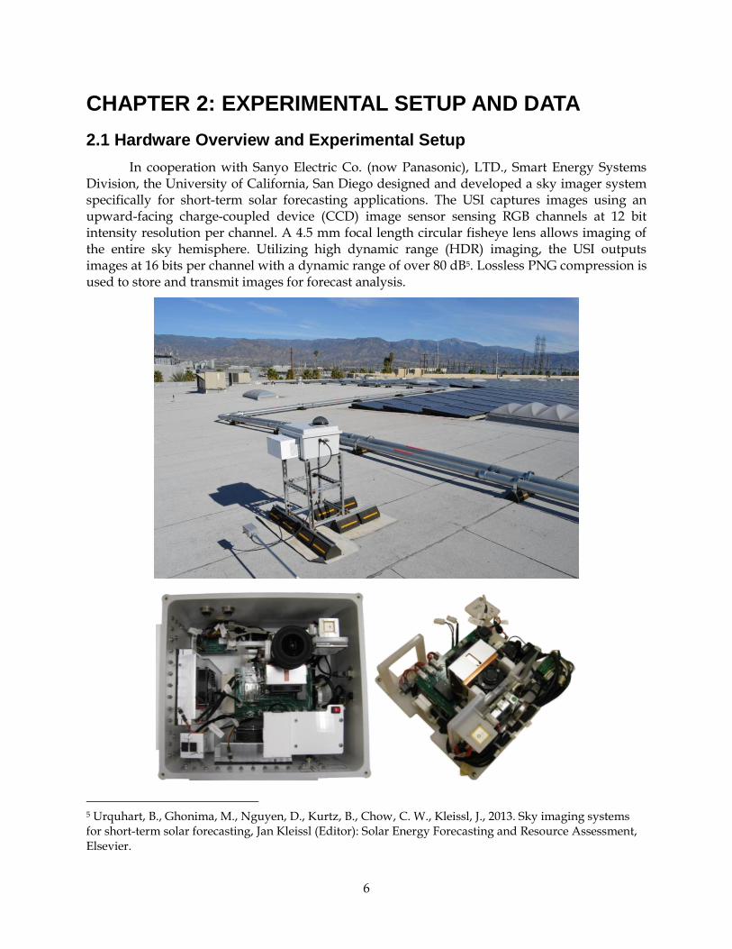
In cooperation with Sanyo Electric Co. (now Panasonic), LTD., Smart Energy Systems Division, the University of California, San Diego designed and developed a sky imager system specifically for short-term solar forecasting applications. The USI captures images using an upward-facing charge-coupled device (CCD) image sensor sensing RGB channels at 12 bit intensity resolution per channel. A 4.5 mm focal length circular fisheye lens allows imaging of the entire sky hemisphere. Utilizing high dynamic range (HDR) imaging, the USI outputs images at 16 bits per channel with a dynamic range of over 80 dB5. Lossless PNG compression is used to store and transmit images for forecast analysis.

5 Urquhart, B., Ghonima, M., Nguyen, D., Kurtz, B., Chow, C. W., Kleissl, J., 2013. Sky imaging systems for short-term solar forecasting, Jan Kleissl (Editor): Solar Energy Forecasting and Resource Assessment, Elsevier.

7

Figure 1: (Top) Final installation of the imager USI1.5 near power plant SPVP011. (Bottom) Overview of the components of the imager

Since cloud cover near the sun provides vital information for short-term solar forecasting, the USI does not employ a solar occulting device. The increased resolution and dynamic range, combined with the ability to image the entire sky hemisphere, has allowed the USI to overcome the primary shortcomings of the TSI system.

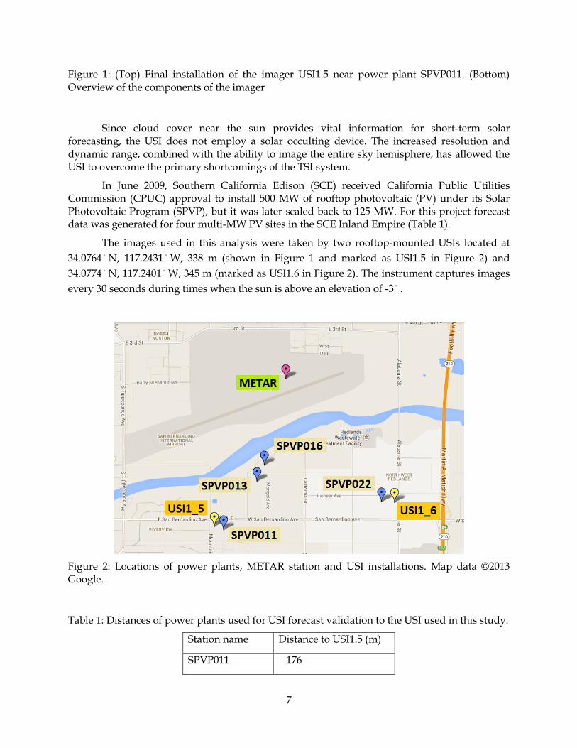
In June 2009, Southern California Edison (SCE) received California Public Utilities Commission (CPUC) approval to install 500 MW of rooftop photovoltaic (PV) under its Solar Photovoltaic Program (SPVP), but it was later scaled back to 125 MW. For this project forecast data was generated for four multi-MW PV sites in the SCE Inland Empire (Table 1).

The images used in this analysis were taken by two rooftop-mounted USIs located at

34.0764 N, 117.2431 W, 338 m (shown in Figure 1 and marked as USI1.5 in Figure 2) and

34.0774 N, 117.2401 W, 345 m (marked as USI1.6 in Figure 2). The instrument captures images

every 30 seconds during times when the sun is above an elevation of -3 .

Figure 2: Locations of power plants, METAR station and USI installations. Map data ©2013 Google.

Table 1: Distances of power plants used for USI forecast validation to the USI used in this study.

Station name Distance to USI1.5 (m)

SPVP011 176

8

SPVP013 1,071

SPVP016 1,277

SPVP022 2,883

METAR 2,804

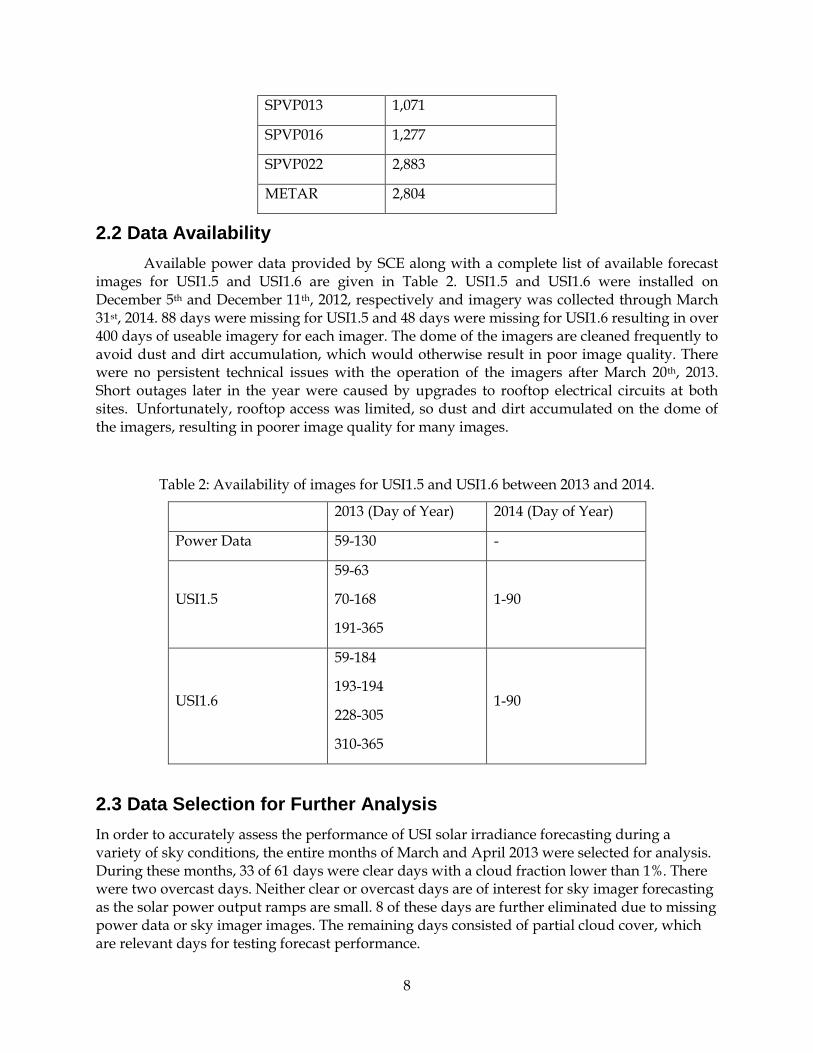
2.2 Data Availability

Available power data provided by SCE along with a complete list of available forecast images for USI1.5 and USI1.6 are given in Table 2. USI1.5 and USI1.6 were installed on December 5th and December 11th, 2012, respectively and imagery was collected through March 31st, 2014. 88 days were missing for USI1.5 and 48 days were missing for USI1.6 resulting in over 400 days of useable imagery for each imager. The dome of the imagers are cleaned frequently to avoid dust and dirt accumulation, which would otherwise result in poor image quality. There were no persistent technical issues with the operation of the imagers after March 20th, 2013. Short outages later in the year were caused by upgrades to rooftop electrical circuits at both sites. Unfortunately, rooftop access was limited, so dust and dirt accumulated on the dome of the imagers, resulting in poorer image quality for many images.

Table 2: Availability of images for USI1.5 and USI1.6 between 2013 and 2014.

2013 (Day of Year) 2014 (Day of Year)

Power Data 59-130 -

USI1.5

59-63

70-168

191-365

1-90

USI1.6

59-184

193-194

228-305

310-365

1-90

2.3 Data Selection for Further Analysis

In order to accurately assess the performance of USI solar irradiance forecasting during a variety of sky conditions, the entire months of March and April 2013 were selected for analysis. During these months, 33 of 61 days were clear days with a cloud fraction lower than 1%. There were two overcast days. Neither clear or overcast days are of interest for sky imager forecasting as the solar power output ramps are small. 8 of these days are further eliminated due to missing power data or sky imager images. The remaining days consisted of partial cloud cover, which are relevant days for testing forecast performance.

9

CHAPTER 3: FORECAST PROCEDURES

3.1 Sky Imager Forecast Procedure

The method used to generate forecasts in this study is an improved implementation of the procedure described in6. A brief overview of the USI forecast procedure will be presented, with a focus on the major improvements made since the previous iteration of UCSD sky imager forecast software. USI forecast data processing may be considered in two main sections: one which operates purely upon sky imager data, and one which is specific to the location and equipment of the site of interest. A forecast may then be issued after all data processing is complete. A graphical guide to help orient the reader in the following sections is provided in Figure 3.

Figure 3: Flowchart of USI forecast procedure.

3.1.1. Geometric calibration and image pre-processing

Before image processing, the USI was calibrated to map each image pixel to a geographic azimuth and zenith angle by leveraging the known position of the sun and the

10

(equisolid angle) projection function of the lens. Once the geographic azimuth and zenith angles are known, a "sun-pixel angle" may be computed as the angle between the vector to the sun and the direction vector for a given image pixel.

After calibration maps have been generated (typically performed once per season or following a maintenance operation), images taken by the USI are cropped to remove static objects on the horizon (buildings, trees, etc.), white balanced by a 3x3 color-correction matrix, and treated for any known sensor errors (e.g. dark current noise).

3.1.2. Detecting clouds

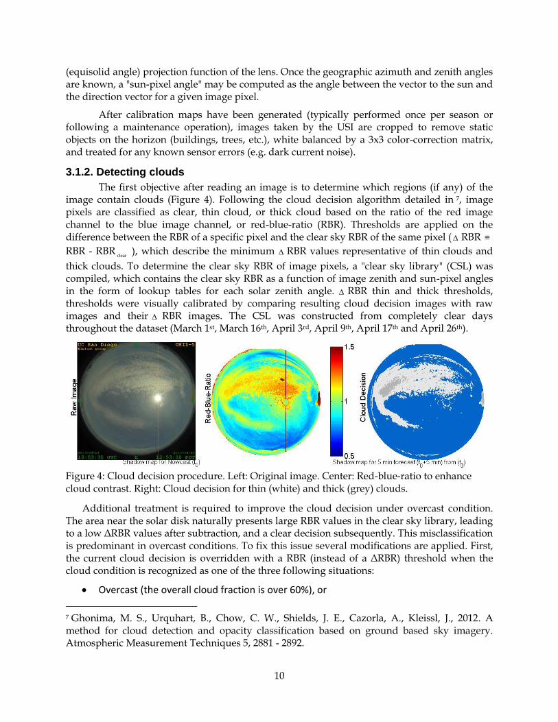
The first objective after reading an image is to determine which regions (if any) of the image contain clouds (Figure 4). Following the cloud decision algorithm detailed in 7, image pixels are classified as clear, thin cloud, or thick cloud based on the ratio of the red image channel to the blue image channel, or red-blue-ratio (RBR). Thresholds are applied on the difference between the RBR of a specific pixel and the clear sky RBR of the same pixel ( RBR

RBR - RBRclear

), which describe the minimum RBR values representative of thin clouds and

thick clouds. To determine the clear sky RBR of image pixels, a "clear sky library" (CSL) was compiled, which contains the clear sky RBR as a function of image zenith and sun-pixel angles in the form of lookup tables for each solar zenith angle. RBR thin and thick thresholds, thresholds were visually calibrated by comparing resulting cloud decision images with raw images and their RBR images. The CSL was constructed from completely clear days throughout the dataset (March 1st, March 16th, April 3rd, April 9th, April 17th and April 26th).

Figure 4: Cloud decision procedure. Left: Original image. Center: Red-blue-ratio to enhance cloud contrast. Right: Cloud decision for thin (white) and thick (grey) clouds.

Additional treatment is required to improve the cloud decision under overcast condition. The area near the solar disk naturally presents large RBR values in the clear sky library, leading to a low ΔRBR values after subtraction, and a clear decision subsequently. This misclassification is predominant in overcast conditions. To fix this issue several modifications are applied. First, the current cloud decision is overridden with a RBR (instead of a ΔRBR) threshold when the cloud condition is recognized as one of the three following situations:

Overcast (the overall cloud fraction is over 60%), or

7 Ghonima, M. S., Urquhart, B., Chow, C. W., Shields, J. E., Cazorla, A., Kleissl, J., 2012. A method for cloud detection and opacity classification based on ground based sky imagery. Atmospheric Measurement Techniques 5, 2881 - 2892.

11

The cloud fraction within the solar disk is larger than 20%, or

The overall cloud fraction is larger than 53% while the cloud fraction within the solar disk is larger than 5% but smaller than 20%.

For the RBR-based cloud decision, the thin and thick thresholds are 1.0 and 1.1, respectively. Second, after applying the cloud decision, the pixels covering the solar disk are reexamined. Saturation is defined for each pixel as the sum of three channel intensities normalized by the sum of the maximum possible values of three channels. Since the pixels in the solar disk are usually saturated if they are unshaded, we assume that a pixel is clear if its saturation is larger than 96%. This improves the cloud decision within the solar disk and therefore improves the nowcast results. The improvement for mostly cloudy conditions with clear sun pixels are illustrated in Figure 5.

Figure 5: Improved cloud decision for nearly overcast conditions. Left: Original image. Center: Red-blue-ratio to enhance cloud contrast. Right: Cloud decision for thin (white) and thick (grey) clouds and clear (blue). For this image, the sun is briefly at least partially unobstructed and the saturation check for pixels within the solar disk correctly clears the solar region.

Direct imaging of the sun also requires additional treatment near the solar disk in order to mitigate cloud decision errors. A "CSL bypass" procedure based on the sunshine parameter used by Chow et al. (2011) was developed: when the sun is determined to be obstructed (less

than 50% saturated pixels in pixels of sun-pixel angle 1< ), the CSL was not used within the

region of sun-pixel angle 35< , and only binary cloud decision was performed by assigning

pixels with RBR > 0.778 as thick clouds.

Finally, markings such as smudges, soiling, and scratches can possess high RBR values, particularly as the position of the sun in the image approaches these markings. A correction algorithm was applied to remove these false small thick clouds. After all cloud decision and correction algorithms have completed, the blooming stripe is addressed. The blooming stripe is detected in the RGB image by searching near the sun for columns of very uniform brightness. If present, the blooming stripe (typically only about 10 pixels wide) is post-processed by interpolating across the edges of the stripe in the cloud decision image (Figure 4).

3.1.3. Cloud height, cloud map, and cloud velocity

Cloud base height (CBH) measurements were obtained from historical weather reports of the standardized METAR weather data format, which are typically generated once per hour

12

(sometimes more frequently) at airports or weather observation stations. In this case, the nearest METAR station was located about 4 km northeast of USI 1_5 at the San Bernardino airport (KSBD). A geometric transform, similar to the pseudo-Cartesian transform of 8 was then performed to map cloud information to a latitude-longitude grid at the CBH. The resulting "cloud map" is a two-dimensional planar mapping of cloud position at the obtained CBH above the forecast site, centered above the physical location of the USI.

Cloud pixel velocity was obtained by applying the cross-correlation method (CCM) to the RBR of two consecutive cloud maps. The vector field resulting from the CCM contains the cloud speed vector field where vectors with small cross-correlation coefficients have been excluded. The vector field is processed through a series of quality controls to yield a single average cloud velocity vector that is applied to the entire cloud map. In other words, the velocity of all clouds is assumed to be identical.

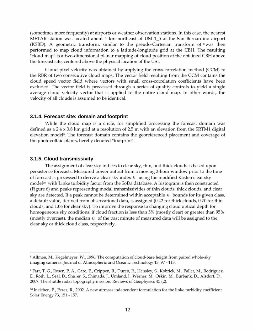
3.1.4. Forecast site: domain and footprint

While the cloud map is a circle, for simplified processing the forecast domain was defined as a 2.4 x 3.8 km grid at a resolution of 2.5 m with an elevation from the SRTM1 digital elevation model9. The forecast domain contains the georeferenced placement and coverage of the photovoltaic plants, hereby denoted "footprint".

3.1.5. Cloud transmissivity

The assignment of clear sky indices to clear sky, thin, and thick clouds is based upon persistence forecasts. Measured power output from a moving 2-hour window prior to the time

of forecast is processed to derive a clear sky index kt using the modified Kasten clear sky model10 with Linke turbidity factor from the SoDa database. A histogram is then constructed (Figure 6) and peaks representing modal transmissivities of thin clouds, thick clouds, and clear

sky are detected. If a peak cannot be determined within acceptable kt bounds for its given class, a default value, derived from observational data, is assigned (0.42 for thick clouds, 0.70 for thin clouds, and 1.06 for clear sky). To improve the response to changing cloud optical depth for homogeneous sky conditions, if cloud fraction is less than 5% (mostly clear) or greater than 95%

(mostly overcast), the median kt of the past minute of measured data will be assigned to the clear sky or thick cloud class, respectively.

8 Allmen, M., Kegelmeyer, W., 1996. The computation of cloud-base height from paired whole-sky imaging cameras. Journal of Atmospheric and Oceanic Technology 13, 97 - 113.

9 Farr, T. G., Rosen, P. A., Caro, E., Crippen, R., Duren, R., Hensley, S., Kobrick, M., Paller, M., Rodriguez, E., Roth, L., Seal, D., Sha_er, S., Shimada, J., Umland, J., Werner, M., Oskin, M., Burbank, D., Alsdorf, D., 2007. The shuttle radar topography mission. Reviews of Geophysics 45 (2).

10 Ineichen, P., Perez, R., 2002. A new airmass independent formulation for the linke turbidity coefficient. Solar Energy 73, 151 - 157.

13

Figure 6: Histogram of measured kt for Nov 14, 2012 10:00:00 PST through 12:00:00 PST, illustrating three distinct peaks representative of thin clouds, thick clouds, and clear sky.

3.1.6. Merge: cloud map advection, shadow map, and irradiance forecast

Irradiance forecasts are produced by advecting the current cloud map at the calculated cloud pixel velocity to generate cloud position forecasts at each forecast interval (30 seconds). The locations of ground shadows cast by clouds as defined by their location in each advected cloud map are determined by ray tracing. The resulting estimation of cloud shadows within the

forecast domain is termed the "shadow map." For each pixel within the footprint, a modal kt is

assigned from the histogram procedure (Section 3.1.5). The average modal kt of the pixels within the power plant is then multiplied by the clear sky power output model to produce plant power output.

3.2 Error Metrics

3.2.1. Cloud map matching metrics

Two quantities were used to characterize the performance of image-based algorithms: matching error and cloud-advection-versus-persistence (cap) error. The 30-sec forecast cloud

map generated at time 0

t was overlaid onto the actual cloud map at time (300t s ) in order to

determine pixel-by-pixel forecast error, or "matching error." No distinction between thin and thick clouds was made in determining matching error; a pixel is either cloudy or clear. Matching error was defined as:

100%.=e

total

false

m

P

P (1)

Matching errors for mostly uniform sky conditions (i.e. completely clear or completely overcast) are by default close to zero and are not an interesting test of forecast skill, so aggregate matching error metrics (e.g. mean and standard deviation) were only computed using matching

14

errors for times corresponding to <5% cloud fraction 95%< . Similarly, daily cap error, scalar average cloud speed, and average cloud height were computed only for the same time periods.

Cap error was computed in order to determine whether cloud advection improves forecast performance compared to a naïve forecast by comparing the number of falsely matched pixels of the 30-sec advection forecasts with those of an image persistence forecast. Image

persistence means that the cloud map at 0

t remains static until 30 seconds later. Cap error was

therefore defined as:

100%.=e

epersistencfalse,

advectionfalse,

cap

P

P (2)

A cap error of less than 100% indicates that cloud advection improves performance over image persistence forecast.

3.2.2. Aggregate error metrics

Time series constructed from 0, 5, 10, and 15 minute forecasts were validated against measured data collected at the four power plants. To avoid disproportional weighting of data near solar noon, validation was also performed on normalized power similar to the clear sky

index kt . Instantaneous power output / kt at the image capture times was used as ground truth.

Four error metrics were used to assess the overall performance of the USI forecast system as a function of forecast horizon: relative mean absolute error (rMAE), relative mean bias error (rMBE), and forecast skill (FS). Relative metrics were obtained by normalizing by the

temporal and spatial average of the observed kt for each day ( kt ). Each metric was computed

for each forecast horizon using kt values averaged across the four power plants. In the following equations, N denotes the total number of forecasts generated on a given day. The superscript "obs" denotes an observed value, and " hf " denotes forecast horizon in minutes

( ,150,0.5,1,= hf min). Therefore, hf

nkt indicates the spatial average of the hf -minute-ahead

clear sky index kt forecasts generated at each power plant at time n

t corresponding to the n th

forecast of the day.

obs

obs

1=

100%1=)(rMAE

kt

ktktN

hfn

hf

n

N

n

(3)

obs

obs

1=

100%1=)(rMBE

kt

ktktN

hfn

hf

n

N

n

(4)

In order to quantify the relative performance of USI forecasts against a reference metric, a forecast skill was calculated for each forecast horizon. Marquez and Coimbra (2013b) found that the ratio of forecast model RMSE to persistence model RMSE is a measure of general forecast skill that is less affected by location, time, and local variability and can therefore be used to intercompare forecast results. The persistence model used was a persistence forecast

generated by assuming power plant measured kt at time n

t persisted for the entire forecast

15

window (i.e. obsepersistenc,

images/

=n

hf

thfnktkt

). Here, rMAE was used to compute forecast skill instead of

rRMSE due to the linear nature of rMAE. Thus, forecast skill FS was defined as

)(rMAE

)(rMAE1=)(FS

phf

hfhf (5)

Positive values of FS therefore indicate USI forecast was superior to power plant persistence forecast, with a maximum possible value of 1.

As an indicator of sample size, the average number of power plants covered by the shadow map for each forecast horizon was computed. Error metrics were not computed for time series showing average number of stations covered less than 1, because the lack of forecast data for the day and forecast horizon in consideration would make the error metrics not representative. Generally plant coverage was not an issue except for March 3rd when the cloud speed was exceptionally high, and thus for longer forecast horizons like 15 minute horizon the cloud map had already moved out of the area covered by the power plants.

3.3 Ramp Events

3.3.1. Ramp Event Detection

One of the major roles that sky imagers can play in solar power integration is to enable and improve the use of ramp mitigation tools. USI forecasts of cloud shadow locations should be able to inform users on timing, magnitude, and duration of upcoming ramp events. This will allow operators to take action to mitigate negative impacts or comply with integration or PPA requirements, especially in areas with high solar penetration.

Ramp rate is defined as the ratio of a certain percentage change in power output over a unit of time, usually minutes. The percentage change is calculated by dividing the change in power output by the nameplate capacity of the power plant. A ramp event is a ramp that exceeds a (arbitrarily defined) critical value. In order to detect ramp events in power and forecast data, each 0 to 15 minutes forecast and corresponding measured power data set were segmented into parts of 1 min duration. Each of the segments is later fitted with a linear polynomial and the fits, which exceeded the preset ramp rate value, were marked as ‘potential ramp event’ (either as ramping up or ramping down event). This procedure was repeated until the starting point of the sub-segments changed to each of the data points in the set one by one. This repetition ensures that a large ramp dataset is created where the choice of specific starting point does not affect the analysis outcome, since the polynomial approximations tend to change slightly with respect to the starting point of the segmentation procedure.

Later, segments marked as potential ramp events which are also neighbors to other marked sub-segments, are appended to each other to form a combined (longer) ramp events. Sample results for a 15 minutes segment are shown in left side of Figure 7.

The combined ramp events may be further processed to ensure certain user-defined conditions. While minimum or maximum duration thresholds were not used, the ramps are cropped to force beginning and end points of the ramp to show more than 2% increase compared to the following /preceding data point.

16

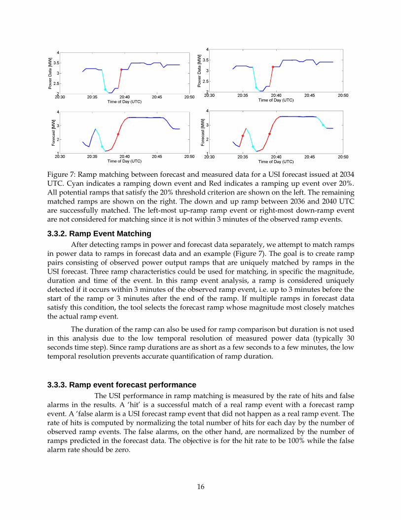
Figure 7: Ramp matching between forecast and measured data for a USI forecast issued at 2034 UTC. Cyan indicates a ramping down event and Red indicates a ramping up event over 20%. All potential ramps that satisfy the 20% threshold criterion are shown on the left. The remaining matched ramps are shown on the right. The down and up ramp between 2036 and 2040 UTC are successfully matched. The left-most up-ramp ramp event or right-most down-ramp event are not considered for matching since it is not within 3 minutes of the observed ramp events.

3.3.2. Ramp Event Matching

After detecting ramps in power and forecast data separately, we attempt to match ramps in power data to ramps in forecast data and an example (Figure 7). The goal is to create ramp pairs consisting of observed power output ramps that are uniquely matched by ramps in the USI forecast. Three ramp characteristics could be used for matching, in specific the magnitude, duration and time of the event. In this ramp event analysis, a ramp is considered uniquely detected if it occurs within 3 minutes of the observed ramp event, i.e. up to 3 minutes before the start of the ramp or 3 minutes after the end of the ramp. If multiple ramps in forecast data satisfy this condition, the tool selects the forecast ramp whose magnitude most closely matches the actual ramp event.

The duration of the ramp can also be used for ramp comparison but duration is not used in this analysis due to the low temporal resolution of measured power data (typically 30 seconds time step). Since ramp durations are as short as a few seconds to a few minutes, the low temporal resolution prevents accurate quantification of ramp duration.

3.3.3. Ramp event forecast performance

The USI performance in ramp matching is measured by the rate of hits and false alarms in the results. A ‘hit’ is a successful match of a real ramp event with a forecast ramp event. A ‘false alarm is a USI forecast ramp event that did not happen as a real ramp event. The rate of hits is computed by normalizing the total number of hits for each day by the number of observed ramp events. The false alarms, on the other hand, are normalized by the number of ramps predicted in the forecast data. The objective is for the hit rate to be 100% while the false alarm rate should be zero.

17

CHAPTER 4: SKY IMAGER FORECAST RESULTS

4.1 Case Studies

USI forecast for two interesting days will now be examined in greater detail to demonstrate the USI's ability to predict major ramp events. These days are April 4th and 16th, 2013. In Figure 8, cloud conditions and respective matching and cap error on April 4th are shown for the power plant SPVP011, where the imager USI1.5 was located. On this day, the morning was overcast with low clouds at 500 m. Since such low clouds limit the view of the USI, the forecast for any of the power plants was not available during that time period. At about 1645 UTC, the sky cleared and for the rest of the day, bands of altocumulus clouds pass over the area.

Figure 8: Cloud conditions on April 4th, 2013 and respective matching and cap error. A cap error of less than 100% indicates forecast improvement (skill) over persistence.

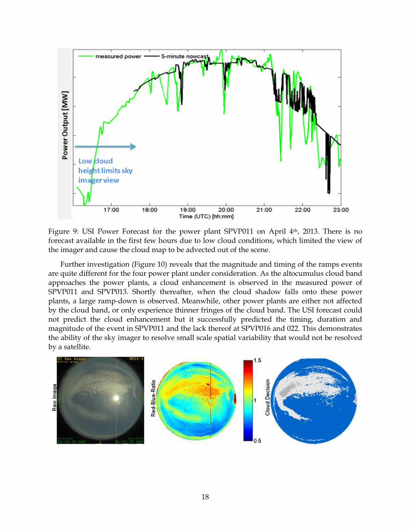
Figure 9 shows the 5 minute power output forecast on April 4th. Most of the timing of the variability in the evening was captured, but most notably, the large ramping down events at 1900 UTC and 2000 UTC were captured well both in timing and duration. The ramp event at 1900 UTC is also captured well in magnitude. A smaller isolated ramp event around 1930 UTC was also correctly predicted.

18

Figure 9: USI Power Forecast for the power plant SPVP011 on April 4th, 2013. There is no forecast available in the first few hours due to low cloud conditions, which limited the view of the imager and cause the cloud map to be advected out of the scene.

Further investigation (Figure 10) reveals that the magnitude and timing of the ramps events are quite different for the four power plant under consideration. As the altocumulus cloud band approaches the power plants, a cloud enhancement is observed in the measured power of SPVP011 and SPVP013. Shortly thereafter, when the cloud shadow falls onto these power plants, a large ramp-down is observed. Meanwhile, other power plants are either not affected by the cloud band, or only experience thinner fringes of the cloud band. The USI forecast could not predict the cloud enhancement but it successfully predicted the timing, duration and magnitude of the event in SPVP011 and the lack thereof at SPVP016 and 022. This demonstrates the ability of the sky imager to resolve small scale spatial variability that would not be resolved by a satellite.

19

Figure 10: Altocumulus cloud band forecast on April 4th, 2013. Raw Image, Red-Blue-Ratio (RBR) and cloud decision at 1953 UTC are shown on top. The power generation forecast for four power plants is given on the bottom. Green line is measured power, black line is USI nowcast, which utilizes cloud decision and projection algorithms to create a “0 minute forecast”. The red line is USI forecast issued at 1953 UTC, which uses nowcast shadow map and cloud velocity to predict the sky conditions up to 15 minutes in advance. To protect the confidentiality of the data, the y axis labels were removed. The ranges are 1.5 MW for SPVP011, 016, and 022 and 2 MW for plant 013.

The forecast skill (Table 5) for April 4th is generally negative at 5 minutes, but becomes positive afterwards. The forecast skill is greatest at SPVP011 but this trend of greater forecast accuracy with proximity to the USI is not persistent when considering all days.

Table 5: rMAE and Forecast Skill for April 4th, 2013

relative Mean Absolute Error (rMAE) [%] Forecast Skill [-]

Forecast Horizon [minutes]

0 5 10 15 5 10 15

Power Error

SPVP 011 4.3 5.1 5.6 5.9 0.0 0.3 0.3

SPVP 013 5.7 6.7 7.2 7.7 -0.3 0.0 0.0

20

SPVP 016 5.0 6.1 6.3 6.7 -0.1 0.1 0.2

SPVP 022 4.9 4.9 5.7 7.1 -0.1 -0.1 -0.1

Average 4.0 4.7 5.4 5.8 -0.1 0.2 0.2

kt Error

SPVP 011 5.7 6.8 7.5 7.8 0.0 0.3 0.3

SPVP 013 7.5 8.9 9.4 10.2 -0.3 0.0 0.0

SPVP 016 7.9 9.8 10.0 10.6 0.0 0.1 0.1

SPVP 022 5.7 5.6 6.5 8.0 0.0 0.0 -0.1

Average 4.6 5.8 6.3 6.9 -0.1 0.1 0.1

April 16th also presents an interesting case study day due to occurrence of both overcast and partly cloudy conditions which lead to large ramps in power output. In Figure 11, cloud conditions and matching and cap error are shown. On this day, the morning was overcast but the cloud decision was still accurate (Figure 12) since the CSL was bypassed in the cloud decision step as discussed in Section 3.1.2. As the sky becomes partly cloudy and clear, the cloud decision automatically reverts back to using the CSL. Throughout the rest of the day, scattered cumulus clouds exist with a tendency to evaporate. The cloud height is constant with one layer until 2100 UTC, and increases to 2500 m in the afternoon.

Figure 11: Cloud conditions on April 16th, 2013 and respective matching and cap error.

21

Figure 12: Cloud decision for overcast conditions on April 16th, 2013. Left: Original image. Center: Red-blue-ratio to enhance cloud contrast. Right: Cloud decision for thin (white) and thick (grey) clouds and clear (blue)

Nowcast power output forecast along with measured power for April 16th is shown in Figure 13. Most of the ramp events in the evening were captured in timing, with a certain degree of magnitude error. At 1900 and 2040 UTC, the large ramp events were captured well both in timing, duration and magnitude. The ramp events after 2100 UTC are also captured well in timing but not as good in magnitude.

Figure 13: USI Power nowcast (0 min forecast) for the power plant SPVP011 on April 16th, 2013. To protect the confidentiality of the data, the y axis labels were removed.

Forecast skill and relative mean absolute error on April 16th is given in Table 6. The forecast skill for this day is generally positive except at SPVP 011. The forecast skill is greatest at SPVP022 and fairly consistent across time horizons.

22

Table 6: rMAE and Forecast Skill for April 16th, 2013

relative Mean Absolute Error (rMAE) [%] Forecast Skill [-]

Forecast Horizon [minutes]

0 5 10 15 5 10 15

Power Error

SPVP 011 10.2 14.2 14.3 18.0 -0.02 0.20 -0.06

SPVP 013 10.7 15.2 17.4 17.5 0.12 0.21 0.10

SPVP 016 12.8 15.9 15.3 16.6 0.13 0.25 0.22

SPVP 022 10.5 13. 14.2 16.2 0.27 0.20 0.22

Average 7.54 10.6 11.9 12.4 0.15 0.22 0.15

4.2. Aggregate results

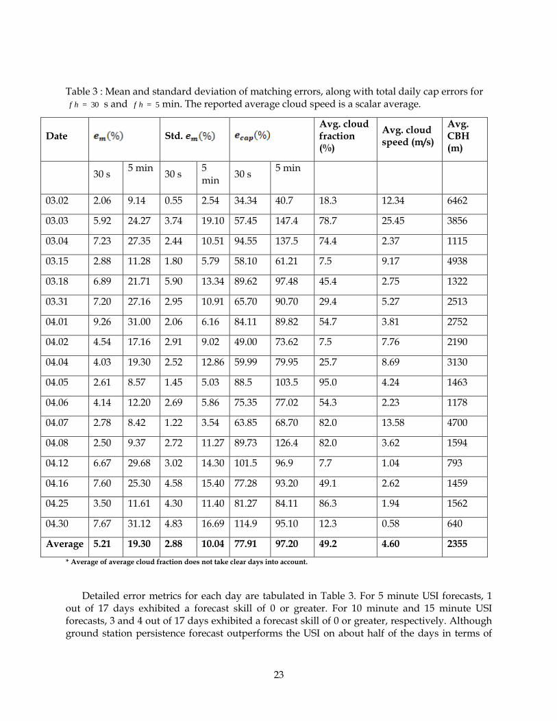
A summary of image-based forecast performance is presented in Table 3 for forecast horizons of 30 seconds and 5 minutes. The average 30-second cap error of 78% suggests that advection was superior to image persistence, but advection performance weakened for 5 min forecast horizons with an average of 97%. Daily cap errors were below 100% for 15 out of 17 days for 30 second forecasts and 13 out of 17 days for 5 minute forecasts. This suggests the underlying principles and assumptions of the cloud decision and cloud velocity algorithms are consistently valid. Days with cap error exceeding 100% demonstrated adverse conditions, such as stationary clouds (advection performs worse than persistence) and very low, rapidly deforming clouds (near 100%, as advection performs just as poorly as persistence).

Compared with the analysis of an idealized dataset of 4 days by Chow et al. (2011), the larger validation set analyzed in this paper (61 consecutive days) presented a wider variety of sky conditions including adverse conditions where the assumption of cloud advection does not hold. This is the main reason for a greater range and larger average cap errors compared to Chow et al. (2011), which ranged from 45.0% to 54.6%. Additionally, new features of the USI such as thin cloud detection and an unobstructed circumsolar region (area immediately surrounding the sun) increase power output forecast skill through greater visibility of the sky

dome and more accurate kt assignment. However, since thin cloud detection fluctuates more from image to image and there are larger cloud decision errors in the circumsolar region, the total number of false pixels in both advection and image persistence forecasts increases, causing their ratio to be closer to unity.

23

Table 3 : Mean and standard deviation of matching errors, along with total daily cap errors for 30=hf s and 5=hf min. The reported average cloud speed is a scalar average.

Date

Std.

Avg. cloud fraction (%)

Avg. cloud speed (m/s)

Avg. CBH (m)

30 s

5 min 30 s

5 min

30 s 5 min

03.02 2.06 9.14 0.55 2.54 34.34 40.7 18.3 12.34 6462

03.03 5.92 24.27 3.74 19.10 57.45 147.4 78.7 25.45 3856

03.04 7.23 27.35 2.44 10.51 94.55 137.5 74.4 2.37 1115

03.15 2.88 11.28 1.80 5.79 58.10 61.21 7.5 9.17 4938

03.18 6.89 21.71 5.90 13.34 89.62 97.48 45.4 2.75 1322

03.31 7.20 27.16 2.95 10.91 65.70 90.70 29.4 5.27 2513

04.01 9.26 31.00 2.06 6.16 84.11 89.82 54.7 3.81 2752

04.02 4.54 17.16 2.91 9.02 49.00 73.62 7.5 7.76 2190

04.04 4.03 19.30 2.52 12.86 59.99 79.95 25.7 8.69 3130

04.05 2.61 8.57 1.45 5.03 88.5 103.5 95.0 4.24 1463

04.06 4.14 12.20 2.69 5.86 75.35 77.02 54.3 2.23 1178

04.07 2.78 8.42 1.22 3.54 63.85 68.70 82.0 13.58 4700

04.08 2.50 9.37 2.72 11.27 89.73 126.4 82.0 3.62 1594

04.12 6.67 29.68 3.02 14.30 101.5 96.9 7.7 1.04 793

04.16 7.60 25.30 4.58 15.40 77.28 93.20 49.1 2.62 1459

04.25 3.50 11.61 4.30 11.40 81.27 84.11 86.3 1.94 1562

04.30 7.67 31.12 4.83 16.69 114.9 95.10 12.3 0.58 640

Average 5.21 19.30 2.88 10.04 77.91 97.20 49.2 4.60 2355

* Average of average cloud fraction does not take clear days into account.

Detailed error metrics for each day are tabulated in Table 3. For 5 minute USI forecasts, 1 out of 17 days exhibited a forecast skill of 0 or greater. For 10 minute and 15 minute USI forecasts, 3 and 4 out of 17 days exhibited a forecast skill of 0 or greater, respectively. Although ground station persistence forecast outperforms the USI on about half of the days in terms of

24

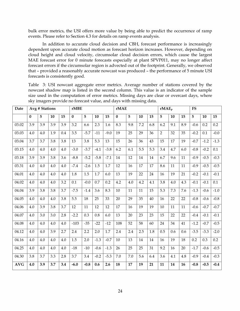
bulk error metrics, the USI offers more value by being able to predict the occurrence of ramp events. Please refer to Section 4.3 for details on ramp events analysis.

In addition to accurate cloud decision and CBH, forecast performance is increasingly dependent upon accurate cloud motion as forecast horizon increases. However, depending on cloud height and cloud velocity, circumsolar cloud decision errors, which cause the largest MAE forecast error for 0 minute forecasts especially at plant SPVP011, may no longer affect forecast errors if the circumsolar region is advected out of the footprint. Generally, we observed that – provided a reasonably accurate nowcast was produced – the performance of 5 minute USI forecasts is consistently good.

Table 3: USI nowcast aggregate error metrics. Average number of stations covered by the nowcast shadow map is listed in the second column. This value is an indicator of the sample size used in the computation of error metrics. Missing days are clear or overcast days, where sky imagers provide no forecast value, and days with missing data.

Date Avg # Stations rMBE rMAE rMAEp FS

0 5 10 15 0 5 10 15 0 5 10 15 5 10 15 5 10 15

03.02 3.9 3.9 3.9 3.9 3.2 6.6 2.3 1.6 8.3 9.8 7.2 6.8 6.2 9.1 8.9 -0.6 0.2 0.2

03.03 4.0 4.0 1.9 0.4 3.5 -5.7 -11 -9.0 19 25 29 36 2 32 35 -0.2 0.1 -0.0

03.04 3.7 3.7 3.8 3.8 13 3.8 5.3 13 15 26 36 43 15 17 19 -0.7 -1.2 -1.3

03.15 4.0 4.0 4.0 4.0 -3.0 -3.7 -4.1 -3.8 6.2 6.1 5.5 5.3 3.4 4.7 6.0 -0.8 -0.2 0.1

03.18 3.9 3.9 3.8 3.6 -8.8 -5.2 -5.8 -7.1 14 12 14 14 6.7 9.6 11 -0.9 -0.5 -0.3

03.31 4.0 4.0 4.0 4.0 -7.4 -2.6 1.5 1.7 12 16 17 17 8.6 11 11 -0.9 -0.5 -0.5

04.01 4.0 4.0 4.0 4.0 1.8 1.5 1.7 6.0 13 19 22 24 16 19 21 -0.2 -0.1 -0.1

04.02 4.0 4.0 4.0 3.2 0.1 -0.0 0.7 0.2 4.2 4.0 4.2 4.1 3.8 4.0 4.3 -0.1 -0.1 0.1

04.04 3.9 3.8 3.8 3.7 -7.5 -1.4 3.6 8.3 10 11 11 15 5.3 7.3 7.6 -1.3 -0.6 -1.0

04.05 4.0 4.0 4.0 3.8 5.5 18 25 33 20 29 35 40 16 22 22 -0.8 -0.6 -0.8

04.06 4.0 3.9 3.8 3.7 12 11 12 12 17 16 19 19 10 11 11 -0.6 -0.7 -0.7

04.07 4.0 3.0 3.0 2.8 -2.2 0.3 0.8 6.0 13 20 23 23 15 22 22 -0.4 -0.1 -0.1

04.08 4.0 4.0 4.0 4.0 -103 -35 -22 -12 108 52 58 60 24 34 41 -1.2 -0.7 -0.5

04.12 4.0 4.0 3.9 2.7 2.4 2.2 2.0 1.7 2.4 2.4 2.5 1.8 0.5 0.6 0.6 -3.5 -3.3 -2.0

04.16 4.0 4.0 4.0 4.0 1.5 2.0 -1.3 -0.7 10 13 14 14 16 19 18 0.2 0.3 0.2

04.25 4.0 4.0 4.0 4.0 -18 -10 -0.6 -1.3 26 25 25 31 9.2 16 20 -1.7 -0.6 -0.5

04.30 3.8 3.7 3.3 2.8 3.7 3.4 -0.2 -5.3 7.0 7.0 5.6 6.4 3.6 4.1 4.8 -0.9 -0.4 -0.3

AVG 4.0 3.9 3.7 3.4 -6.0 -0.8 0.6 2.6 18 17 19 21 11 14 16 -0.8 -0.5 -0.4

25

4.3. Ramp rate distribution

The variability of the power output can be visualized as a cumulative distribution function (CDF) of ramp rates, which are defined as

nameplatetP

tPttP

)()(=RR , (6)

where <> indicates a moving average over Δt, Pnameplate is the nameplate capacity of the respective power plant. Figure 14 shows the cumulative distribution functions of the measurement data. Over one 1 min time steps, ramp rates range up to 25% per minute in SPVP011, 32% per minute in SPVP013, 46% per minute in SPVP016 and 27% per minute in SPVP022. Over 10 min time steps, ramp rates are less than 10% per minute in SPVP011 (which corresponds to 100% over the 10 min time step), 5% per minute in SPVP013, 7% per minute in SPVP016 and 6% per minute in SPVP022. While 10 minute ramps do not differ significantly by power plants size as they are driven by larger cloud systems, 1 minute ramps are a strong function of capacity. The smallest plant (SPVP016) shows almost twice the largest relative 1 min ramps compared to the largest plant.

Figure 14: Cumulative distribution function of ramp rates in power output at 1 minute and 10 minutes intervals for data from Feb 28, 2013 to May 10, 2013. Ramp rates are normalized by

26

plant DC capacity. In other words, a 10% ramp rate corresponds to 500 kW min-1 for SPVP011, 490 kW min-1 for SPVP013, 175 kW min-1 for SPVP016 and 310 kW min-1 for SPVP022.

4.4. Ramp event detection

The results for hits and false alarms are shown with error bars in Figure 15. The results are grouped by forecast horizon (0 to 5, 5 to 10, and 10 to 15 min) based on the start time of the ramp.

Figure 15: Overall performance of USI forecast in predicting ramp events over 15%. Error bars represent the interquartile range of hit and false alarm percentage among different days

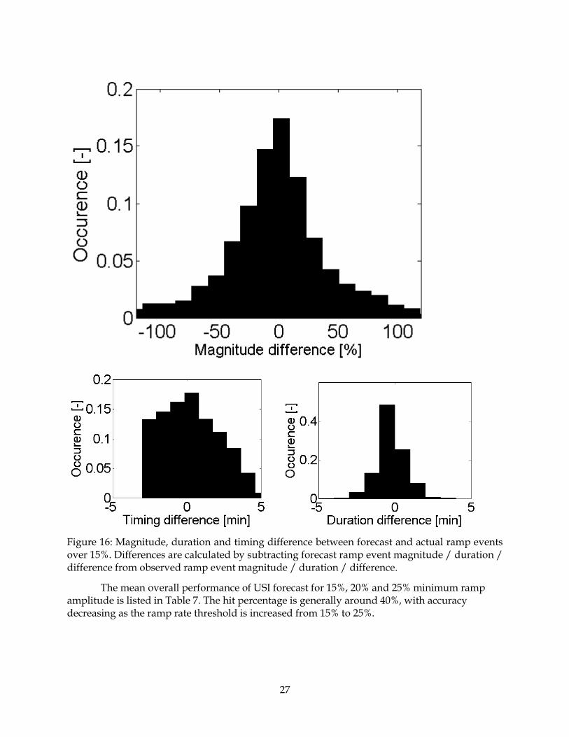
Magnitude, duration and timing differences are another way to evaluate forecast performance. Sample results for 15% ramp events are shown in Figure 16. The magnitude difference indicates how much larger/smaller the forecast ramp is predicted compared to the observed ramp. Duration difference indicates how much longer/shorter the forecast ramp is compared to the observed ramp. Note that the utility of the duration metric is limited, since the data resolution is around 0.6 data points per minute. Nevertheless, it is being reported for reference. Finally, the timing difference indicates how late/early the beginning of a forecast ramp event is predicted compared to the observed ramp. Accurate prediction of the ramp event timing directly influences the operator’s ability to react to an upcoming ramp, and therefore, this information is usually more valuable than the other two metrics.

27

Figure 16: Magnitude, duration and timing difference between forecast and actual ramp events over 15%. Differences are calculated by subtracting forecast ramp event magnitude / duration / difference from observed ramp event magnitude / duration / difference.

The mean overall performance of USI forecast for 15%, 20% and 25% minimum ramp amplitude is listed in Table 7. The hit percentage is generally around 40%, with accuracy decreasing as the ramp rate threshold is increased from 15% to 25%.

28

Table 7: Mean overall performance of USI forecast in predicting ramp events over 15%, 20% and 25% of all power plants and over all XX days.

Minimum ramp amplitude

Average # of observed ramps

Average # of forecast ramps

Mean Overall Hit [%]

Mean Overall False Alarm [%]

15% 973 1033 43.8 67.2

20% 875 950 38.9 74.6

25% 781 841 38.8 79.7

The directional tendency of magnitude, duration and timing differences are assessed via the mean bias error (MBE). The typical deviation from zero error for each variable is analyzed by using mean absolute error (MAE)

forecastobs

N

n

rrN

1=

1=MBE (7)

forecastobs

N

n

rrN

1=

1=MAE

,

(8)

where r is the quantity in question.

MBE and MAE are given in Table 8. The results show that forecasts have a tendency of predicting smaller magnitude which likely stems from the inability of the sky imager to forecast cloud enhancement, i.e. exceedance of clear sky irradiance which often precedes or proceeds large ramp events. The timing and duration error biases are within the uncertainty of the temporal resolution of the data and are therefore insignificant. The magnitude difference has an overall mean of 45-50%, the duration difference is around 0.5 minute and the prediction is made usually 1.5-2 minutes off compared to the actual event.

Table 8: Overall performance of USI forecast in predicting ramp events over 15%, 20% and 25%. The difference is defined as forecast minus measured.

Magnitude Difference [%] Duration Difference [min]

Timing Difference [min]

Ramp Magnitude

MBE MAE MBE MAE MBE MAE

Over 15% -6.99 44.3 -0.17 0.71 0.23 1.70

Over 20% -7.36 48.4 -0.10 0.54 0.18 1.65

Over 25% -6.57 49.5 -0.12 0.43 0.10 1.63

The principal limitation of this analysis comes from the nature of the available data. Usually, ramp rate events in solar power plants of a few MW in size occur over a few seconds to

29

a minute, which is the time it takes for a cloud to move over the plant. Unfortunately, the temporal resolution used in this study is only 1183 data points per day on average, which corresponds to a timestep of about 36 seconds, on average. This low resolution limits testing of USI performance for the typical short ramp events. The low resolution also affects the ability to detect and match ramps, since there is no possibility of using detailed temporal evolution of a ramp (i.e. the shape of a ramp) to compare observed events with forecast events. Instead, the low resolution results in similar ramp profiles with sharp slope changes between pairs of data points.

4.5. Forecast improvements through cloud height correction

An interesting finding on April 16th, 2013 data is that when the METAR cloud height data is adjusted through an optimization procedure, there is a large improvement in the forecast, especially in nowcast curves. Figure 17 shows the nowcast results generated with the cloud height data from METAR (black, 1433 m) and with corrected cloud height data (red, 1733 m). With the corrected cloud height, the ramping down events around 1910 UTC for plants SPVP 013 and SPVP 016 are captured with great accuracy. For other time periods, similar improvements are observed primarily in ramp magnitude, but also in ramp timing.

Cloud height corrections have not been performed in the remainder of this report, since each instance requires manual inspection to ensure improvements in the forecast. Moreover, it is difficult to justify adjustments in the cloud height data without actual measurements. The improvement could simply be a result of ‘overfitting’ the nowcasts to the measurements and may not actually result in improved forecasts. The nearby METAR site is the only local source of cloud height data. The close proximity of the METAR station and the relatively flat terrain constitute a best-case scenario for cloud height accuracy. Nevertheless, cloud heights are only provided every hour and in practice significant intra-hour variability can occur. We speculate that on-site cloud height measurements should drastically improve the accuracy of USI forecasts.

30

Figure 17: Nowcast analysis for a short segment around noon LST on Apr 16th 2013 with cloud height of 1433 m from METAR (black) and 1733 m after the correction (red). To protect the confidentiality of the data, the y axis labels were removed.

31

CHAPTER 5: SATELLITE FORECAST PERFORMANCE

5.1 Satellite Data Overview

Clean Power Research (CPR) provided us with satellite forecast data around the four SPVP sites. The satellite data used in this analysis were centered at 34° 4' 30" N, 117° 14' 42"W (marked as satellite pixel 1 in Figure 18) and 34° 5' 6"N, 117° 14' 6"W (satellite pixel 2 in Figure 18). The spatial coverage of 0.01 degrees for longitude and latitude, which corresponds to about 1 km x 1 km is marked as a red square in Figure 18. SPVP011 was contained in pixel 1, and SPVP013 and SPVP016 were contained in pixel 2. Satellite forecasts are issued with every new satellite image twice per hour at :00 and :30 min and the temporal resolution of the forecast horizon is 1 minute out to 30 min. Linear interpolation was used to calculate the forecast GHI every 30 seconds consistent with the sky imager forecasts.

Figure 18: Locations of satellite pixels (red squares) relative to power plants. Map data ©2012 Google Earth.

5.2 Satellite data selection for analysis

Satellite data were available for all of 2013, while available power plant and USI data are catalogued in Table 9. USI and satellite forecasts were both available for the 17 days that were not clear or overcast in March and April 2013 (Table 10) and the comparison was performed over this period.

Table 9: Availability of power data, USI images, and satellite data.

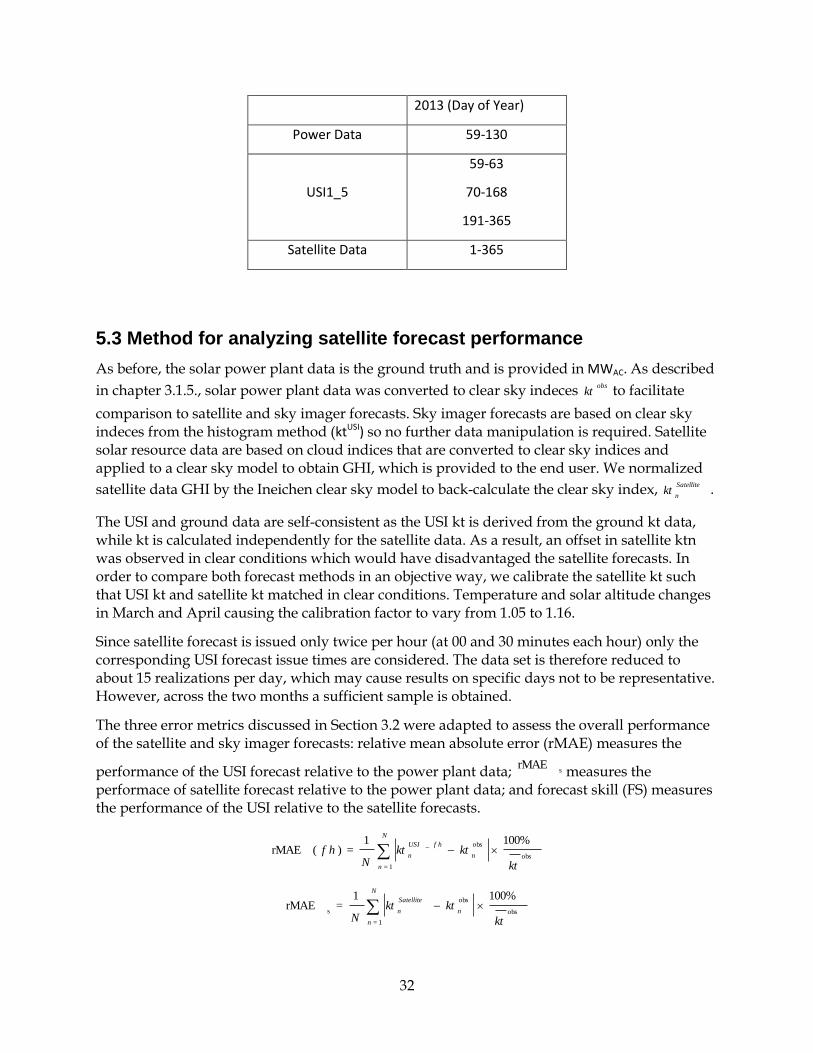
32

2013 (Day of Year)

Power Data 59-130

USI1_5

59-63

70-168

191-365

Satellite Data 1-365

5.3 Method for analyzing satellite forecast performance

As before, the solar power plant data is the ground truth and is provided in MWAC. As described

in chapter 3.1.5., solar power plant data was converted to clear sky indeces obskt to facilitate

comparison to satellite and sky imager forecasts. Sky imager forecasts are based on clear sky indeces from the histogram method (ktUSI) so no further data manipulation is required. Satellite solar resource data are based on cloud indices that are converted to clear sky indices and applied to a clear sky model to obtain GHI, which is provided to the end user. We normalized

satellite data GHI by the Ineichen clear sky model to back-calculate the clear sky index, Satellite

nkt .

The USI and ground data are self-consistent as the USI kt is derived from the ground kt data, while kt is calculated independently for the satellite data. As a result, an offset in satellite ktn was observed in clear conditions which would have disadvantaged the satellite forecasts. In order to compare both forecast methods in an objective way, we calibrate the satellite kt such that USI kt and satellite kt matched in clear conditions. Temperature and solar altitude changes in March and April causing the calibration factor to vary from 1.05 to 1.16.

Since satellite forecast is issued only twice per hour (at 00 and 30 minutes each hour) only the corresponding USI forecast issue times are considered. The data set is therefore reduced to about 15 realizations per day, which may cause results on specific days not to be representative. However, across the two months a sufficient sample is obtained.

The three error metrics discussed in Section 3.2 were adapted to assess the overall performance of the satellite and sky imager forecasts: relative mean absolute error (rMAE) measures the

performance of the USI forecast relative to the power plant data; srMAE

measures the performace of satellite forecast relative to the power plant data; and forecast skill (FS) measures the performance of the USI relative to the satellite forecasts.

obs

obs_

1=

100%1=)(rMAE

kt

ktktN

hfn

hfUSI

n

N

n

obs

obs

1=

s

100%1=rMAE

kt

ktktN

n

Satellite

n

N

n

33

srMAE

)(rMAE1=

hfFS

SatUSI

.

Positive values of FS therefore indicate USI forecast was superior to satellite forecast, with a maximum possible value of 1.

5.4 Satellite forecast performance compared to USI forecast

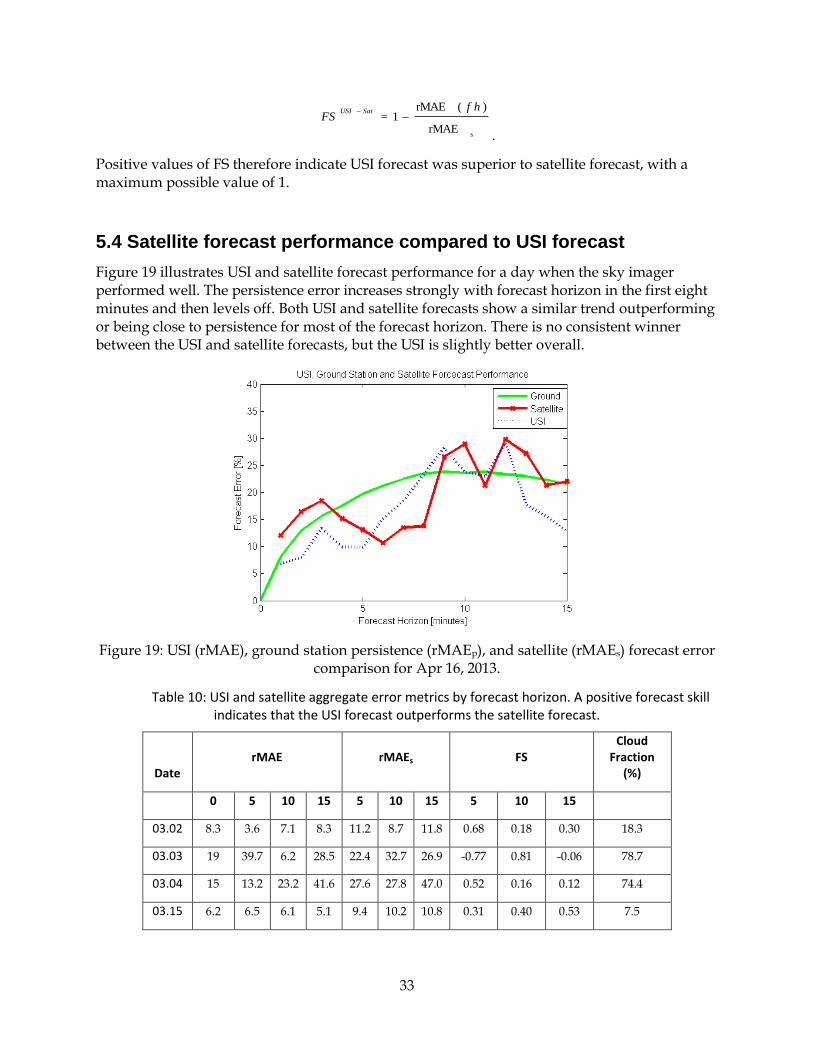
Figure 19 illustrates USI and satellite forecast performance for a day when the sky imager performed well. The persistence error increases strongly with forecast horizon in the first eight minutes and then levels off. Both USI and satellite forecasts show a similar trend outperforming or being close to persistence for most of the forecast horizon. There is no consistent winner between the USI and satellite forecasts, but the USI is slightly better overall.

Figure 19: USI (rMAE), ground station persistence (rMAEp), and satellite (rMAEs) forecast error comparison for Apr 16, 2013.

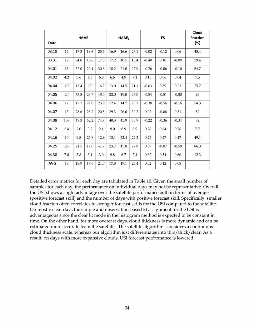
Table 10: USI and satellite aggregate error metrics by forecast horizon. A positive forecast skill indicates that the USI forecast outperforms the satellite forecast.

Date rMAE rMAEs FS

Cloud Fraction

(%)

0 5 10 15 5 10 15 5 10 15

03.02 8.3 3.6 7.1 8.3 11.2 8.7 11.8 0.68 0.18 0.30 18.3

03.03 19 39.7 6.2 28.5 22.4 32.7 26.9 -0.77 0.81 -0.06 78.7

03.04 15 13.2 23.2 41.6 27.6 27.8 47.0 0.52 0.16 0.12 74.4

03.15 6.2 6.5 6.1 5.1 9.4 10.2 10.8 0.31 0.40 0.53 7.5

34

Date rMAE rMAEs FS

Cloud Fraction

(%)

03.18 14 17.3 18.6 25.5 16.9 16.6 27.1 -0.02 -0.12 0.06 45.4

03.31 12 24.0 16.6 17.8 17.2 18.5 16.4 -0.40 0.10 -0.08 29.4

04.01 13 32.0 22.4 30.6 18.2 21.0 27.9 -0.76 -0.06 -0.10 54.7

04.02 4.2 5.6 4.6 6.8 6.6 4.9 7.1 0.15 0.06 0.04 7.5

04.04 10 13.4 6.0 16.2 13.0 14.5 21.1 -0.03 0.59 0.23 25.7

04.05 20 33.8 28.7 48.5 22.0 19.0 27.0 -0.54 -0.51 -0.80 95

04.06 17 17.1 22.8 23.9 12.4 14.7 20.7 -0.38 -0.56 -0.16 54.3

04.07 13 28.6 28.2 20.8 29.3 26.6 30.2 0.02 -0.06 0.31 82

04.08 108 49.3 62.2 74.7 40.3 45.9 55.9 -0.22 -0.36 -0.34 82

04.12 2.4 2.0 3.2 2.1 9.0 8.9 8.9 0.78 0.64 0.76 7.7

04.16 10 9.8 23.8 12.9 13.1 32.4 24.3 0.25 0.27 0.47 49.1

04.25 26 21.5 17.0 41.7 23.7 15.8 27.8 0.09 -0.07 -0.50 86.3

04.30 7.0 3.8 3.1 3.0 9.8 6.7 7.4 0.62 0.54 0.60 12.3

AVG 18 18.9 17.6 24.0 17.8 19.1 23.4 0.02 0.12 0.08

Detailed error metrics for each day are tabulated in Table 10. Given the small number of samples for each day, the performance on individual days may not be representative. Overall the USI shows a slight advantage over the satellite performance both in terms of average (positive forecast skill) and the number of days with positive forecast skill. Specifically, smaller cloud fraction often correlates to stronger forecast skills for the USI compared to the satellite. On mostly clear days the simple and observation-based kt assignment for the USI is advantageous since the clear kt mode in the histogram method is expected to be constant in time. On the other hand, for more overcast days, cloud thickness is more dynamic and can be estimated more accurate from the satellite. The satellite algorithms considers a continuous cloud thickness scale, whereas our algorithm just differentiates into thin/thick/clear. As a result, on days with more expansive clouds, USI forecast performance is lowered.

35

CHAPTER 6: CONCLUSIONS

For the first time, the forecast performance of the newly developed UCSD sky imager (USI) has been analyzed. Sky imagers were deployed for a year at a distribution feeder with four utility-scale warehouse rooftop solar power plants owned by Southern California Edison (SCE). Sky imager data and power output were available every 30 seconds. The largest 1 min ramps in power output were 46% of DC capacity for the smallest 1.7 MW plant, while the largest plant (5 MW) only showed ramps up to 25% of PV capacity.

Zero to fifteen minute power output forecasts for each of the four rooftop power plants were investigated over two months and two days were analyzed in greater depth. The difficulty of accurate cloud detection in the solar region causes sky imager forecast errors to be larger for 5 minute horizons. Forecast skill relative to persistence forecasts improves for longer horizons. Specific examples of promising ramp forecast skills were presented, but inaccuracies in cloud height limit ramp forecast accuracy.

USI forecast performance is also analyzed against a 1 minute resolution satellite forecast. The forecast errors are comparable with slight advantages for the USI. Further improvements in sky imager forecasts will require more accurate atmospheric input measurements of cloud height and cloud optical depth and application of advanced machine learning tools.