© 2018 Institute of Physics and Engineering in Medicine

1. Introduction

In emission tomography, and particularly in positron emission tomography (PET), tomographic reconstruction algorithms implemented by medical imaging manufacturers estimate the 3D map of a radio-tracer concentration without systematic estimation of the uncertainty associated with the reconstructed voxel activities. Yet decision procedures based on quantitative analysis of images would benefit from such uncertainty estimates. The methods currently used for comparing activity values in different regions of interest (ROI) are mostly empirical. Associating a confidence interval with each estimated value would enable a statistical comparison based on hypothesis testing. For instance, in the context of patient monitoring, a physician would be able to perform an objective statistical analysis to compare two ROIs in the same image or in two images reconstructed at two different time points.

Uncertainties associated with reconstructed activity values can actually be estimated using numerous approaches. The first set of approaches consists of propagating the known variance of measurements to the variance and covariance of the reconstructed values. This is usually based on the assumption that the meas-urements follow a Poisson distribution. Methods have been described in Fessler (1996), Qi and Leahy (2000), Stayman and Fessler (2004) and Li (2011) for the penalized likelihood maximization (PLM) algorithm, or equivalently for the maximum a posteriori (MAP) algorithm; Barrett et al (1994a) and Barrett et al (1994b) for the maximum likelihood—expectation maximization (ML-EM) method; Higdon et al (1997) and Sitek (2012) for Bayesian estimates; Sitek (2008) for the origin ensembles method and (Soares et al 2000, 2005) for block-iterative methods. The second set of approaches does not require any assumption regarding the statisti-cal properties of the measured data. It uses bootstrap resampling to produce replicates that are then used to determine the statistical properties of the activity values (Buvat 2002, Dahlborn 2001, Lartizien et al 2010). The common point between these methods is that they usually describe the statistical variability using the variance or standard deviation estimate. As the statistical distribution of the reconstructed image is not neces-sarily Gaussian, confidence intervals cannot be constructed in a straightforward way from these estimates. Moreover, all of these approaches are computationally demanding and difficult to implement in routine clinical applications.

F Kucharczak et al

Interval-based reconstruction for uncertainty quantification in PET

Printed in the UK

035014

PHMBA7

© 2018 Institute of Physics and Engineering in Medicine

63

Phys. Med. Biol.

PMB

1361-6560

10.1088/1361-6560/aa9ea6

3

1

13

Physics in Medicine & Biology

IOP

25

January

2018

Interval-based reconstruction for uncertainty quantification in PET

Florentin Kucharczak1,2,4, Kevin Loquin1, Irène Buvat3, Olivier Strauss1 and Denis Mariano-Goulart4

1 LIRMM, Univ. Montpellier, CNRS, France2 Siemens Healthineers, Saint-Denis, France3 Imagerie Moléculaire In Vivo, UMR 1023 Inserm/CEA/Université Paris Sud - ERL 9218 CNRS, CEA Service Hospitalier Frédéric Joliot,

Orsay, France4 Department of Nuclear Medicine, Montpellier University Hospital and PhyMedExp, University of Montpellier, INSERM U1046, CNRS

UMR 9214, Montpellier, France

E-mail: florentin.kucharczak@lirmm.fr

Keywords: uncertainty quantification, statistical estimation, image reconstruction, non-additive modeling, emission tomography, system matrix

AbstractA new directed interval-based tomographic reconstruction algorithm, called non-additive interval based expectation maximization (NIBEM) is presented. It uses non-additive modeling of the forward operator that provides intervals instead of single-valued projections. The detailed approach is an extension of the maximum likelihood—expectation maximization algorithm based on intervals. The main motivation for this extension is that the resulting intervals have appealing properties for estimating the statistical uncertainty associated with the reconstructed activity values. After reviewing previously published theoretical concepts related to interval-based projectors, this paper describes the NIBEM algorithm and gives examples that highlight the properties and advantages of this interval valued reconstruction.

PAPER2018

RECEIVED 26 May 2017

REVISED

29 November 2017

ACCEPTED FOR PUBLICATION

1 December 2017

PUBLISHED 25 January 2018

https://doi.org/10.1088/1361-6560/aa9ea6Phys. Med. Biol. 63 (2018) 035014 (13pp)

2

F Kucharczak et al

The approach presented in this paper involves direct estimation of confidence intervals associated with activity values. Note that here we only focus on providing an estimate of the uncertainty induced by statistical variations in the measurements. Other sources of uncertainty (eg, associated with the scatter estimate) are not addressed in this paper. We describe a new reconstruction paradigm in which the error is estimated as part of the reconstruction process. Our algorithm, called non-additive interval based expectation maximization (NIBEM), is an extension of the usual ML-EM algorithm. It uses non-additive modeling of the measuring process to build a forward projec-tion operator that generates intervals instead of precise values. This operator has already been described in Rico et al (2009). In the aforementioned paper, the authors stressed that using this kind of projection operator leads to projected intervals whose width is closely correlated with the level of noise of the projected central image. Here we extend the work of Rico et al (2009) to make those operators compatible with a multiplicative reconstruction algo-rithm such as ML-EM, which is, with its variants, the most widespread algorithm in PET clinical routine, by using directed interval arithmetic (Markov 1996). Some very preliminary results were briefly presented in the abstract (Loquin et al 2014). In this paper, using analytical simulations and GATE (Jan et al 2004) simulations, we show that NIBEM provides a practical approximation of confidence intervals associated with reconstructed values.

2. Radon matrix modeling and imprecision

The approach we present here is formulated for 2D reconstructions. The extension to 3D is straightforward when ignoring border effects due to the limited field of view of the tomograph.

Reconstructing a tomographic image involves inverting a model that projects the values of each pixel of the unknown image to the measured projections. As this projection model is usually supposed to be linear, this involves a system matrix R, also called a Radon matrix, whose (i, j)th element can be interpreted as the probability of a photon emitted in the ith pixel to reach the jth detector6. Let f be the n × 1 vector of the pixel values of the image to be reconstructed and let p be the m × 1 measurement vector, then the linear projection operator P based on the system matrix R is defined by:

pj = P( f )j =n∑

i=1

Ri,jfi. (1)

Most reconstruction methods make use of the dual operator of the projection operator called the back- projection operator B defined by:

fi = B( p)i =

m∑j=1

Ri,jpj. (2)

Many different models of the system matrix have been proposed in the relevant literature that account for different ways of modeling the interplay (Unser et al 1993) between the discrete reconstruction space and the continuous space, where the problem can be formulated. On one hand, continuous-to-discrete interplay is modeled by describing how the detector measures the projected activity. We call this the measurement model (MM). On the other hand, discrete-to-continuous interplay involves interpolation kernels. For example, a near-est neighbor interpolation kernel associated with a Dirac MM leads to the line-length model (Wernick and Aarsvold 2004), while rectangular modeling of the measurement with the same interpolation leads to the con-cave disk model (Huesman et al 1977).

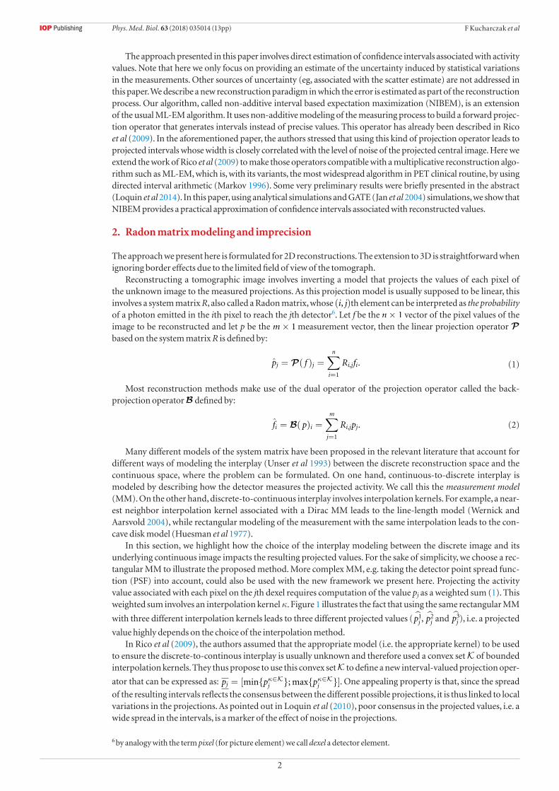
In this section, we highlight how the choice of the interplay modeling between the discrete image and its underlying continuous image impacts the resulting projected values. For the sake of simplicity, we choose a rec-tangular MM to illustrate the proposed method. More complex MM, e.g. taking the detector point spread func-tion (PSF) into account, could also be used with the new framework we present here. Projecting the activity value associated with each pixel on the jth dexel requires computation of the value pj as a weighted sum (1). This weighted sum involves an interpolation kernel κ. Figure 1 illustrates the fact that using the same rectangular MM

with three different interpolation kernels leads to three different projected values ( p1j , p

2j and p3

j ), i.e. a projected

value highly depends on the choice of the interpolation method.In Rico et al (2009), the authors assumed that the appropriate model (i.e. the appropriate kernel) to be used

to ensure the discrete-to-continous interplay is usually unknown and therefore used a convex set K of bounded interpolation kernels. They thus propose to use this convex set K to define a new interval-valued projection oper-

ator that can be expressed as: pj = [minpκ∈Kj ; maxpκ∈K

j ]. One appealing property is that, since the spread

of the resulting intervals reflects the consensus between the different possible projections, it is thus linked to local variations in the projections. As pointed out in Loquin et al (2010), poor consensus in the projected values, i.e. a wide spread in the intervals, is a marker of the effect of noise in the projections.

6 by analogy with the term pixel (for picture element) we call dexel a detector element.

Phys. Med. Biol. 63 (2018) 035014 (13pp)

3

F Kucharczak et al

Computing this interval-valued projection can appear to be computationally complex since no pair of inter-polation kernels can provide the extreme values of every set pj . A Monte-Carlo-like approach could be used, however, this would be very time consuming and would only provide an inner approximation of the two extreme points. The solution proposed in Rico et al (2009) uses the notion of concave capacities. We explain in section 3 how this solution can be used to define an interval valued projection operator that accounts for the supposed imprecise knowledge on this appropriate interpolation kernel.

3. Non-additive construction of the forward projection operator

This section explains how a concave capacity (Denneberg 1994) can be used to model imprecise knowledge regarding the most appropriate interpolation model (Rico et al 2009). As previously, we choose a rectangular MM for didactic purposes and show that the method can be seen as a non-additive extension of the concave disk model.

3.1. A concave capacity to define the geometric interaction between pixels and dexelsLet Ω be a reference set (e.g. 1, . . . , n). A concave capacity ν is a non-additive confidence measure, i.e. a weight associated with any subset of Ω. It extends the notion of probability measure since it does not follow the additive axiom, i.e. ∀A, B ⊆ Ω, ν(A) + ν(B) ν(A ∪ B) + ν(A ∩ B), while a probability measure P would verify P(A) + P(B) = P(A ∪ B) + P(A ∩ B) : a probability measure is an additive confidence measure. Let Λ(Ω) be the set of all probability measures on Ω. It has been shown in Denneberg (1994) and Schmeidler (1986) that a concave capacity ν encodes a convex subset of Λ(Ω) called the core of ν and is denoted M(ν):

M(ν) = P ∈ Λ(Ω) | ∀A ⊆ Ω, P(A) ∈ [νc(A), ν(A)], (3)

where νc is the dual capacity of ν defined by : ∀A ⊆ Ω, νc(A) = ν(Ω)− ν(Ac), with Ac being the complementary set of A in Ω. By construction, νc is convex (Rico and Strauss 2010) (i.e. νc(A) + νc(B) νc(A ∪ B) + νc(A ∩ B)).

Let us now call Tj the tube of response (TOR) associated with the jth dexel of the measurement vector (i.e. the MM is assumed to be a rectangular function). Then, the confidence measure (i.e. the weight) associated with the interaction between the ith pixel and the jth dexel can be expressed as:

Ri,j =| Ci ∩ Tj |, (4)

where | · | is the Lebesgue measure. This is the concave disk model. Let A be a subset of Ω. The confidence measure Pj(A) associated with the interaction between A and the jth dexel is defined by Pj(A) =

∑i∈A Ri,j. The thus-

defined confidence measure is additive, since ∀i = i′, Ci ∩ Ci′ = ∅.Let us consider the four pixel discrete image depicted in figure 2(a) with Ω = 1, 2, 3, 4. With the usual

(additive) modeling of the interaction between pixels and dexels, the domain Ci associated with the ith pixel is obtained by partitioning the continuous domain as illustrated in figure 2(a). With this partitioning, ∀i = i′, Ci ∩ Ci′ = ∅ and

⋃i∈Ω Ci covers the entire continuous domain. Each domain Ci can be considered

as being generated by the rectangular kernel κr that defines the nearest neighbor interpolation: let ωi be the

center of Ci, then Ci = ω ∈ R2,κr(ω − ωi) = 1. Thus, the continuous value f (ω) associated with a loca-

tion ω in the continuous domain is defined by f (ω) = fi, where i is the only value of Ω such that ω ∈ Ci (i.e. κr(ω − ωi) = 1).

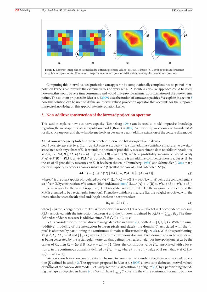
We now show how a concave capacity can be used to compute the bounds of the jth interval-valued projec-tion pj defined in section 2. The approach proposed in Rico et al (2009) allows us to define an interval-valued extension of the concave disk model. Let us replace the usual partitioning of figure 2(a) by a partitioning includ-ing overlaps as depicted in figure 2(b). We still have

⋃i∈Ω Ci covering the entire continuous domain, but now

(a) (b) (c) (d)

Figure 1. Different interpolation kernels lead to different projected values. (a) Discrete image. (b) Continuous image for nearest neighbor interpolation. (c) Continuous image for bilinear interpolation. (d) Continuous image for bicubic interpolation.

Phys. Med. Biol. 63 (2018) 035014 (13pp)

4

F Kucharczak et al

∃i = i′, Ci ∩ Ci′ = ∅. This partitioning can be considered as being generated by a rectangular kernel ηr that is larger than κr . This leads to an imprecise extension of the nearest neighbor interpolation: the interpolated con-

tinuous activity values at location ω is interval-valued and defined by f (ω) = [mini∈N (ω) fi;maxi∈N (ω) fi], where N (ω) ⊆ Ω is the set of neighbors of ω defined by: N (ω) = i ∈ Ω | ηr(ω − ωi) = 1. f (ω) is the set of all

the values that can be obtained by a normalized weighted sum of the nearest neighbors of ω. The proposed model no longer coincides with the concave disk model but defines a concave capacity νj that can be considered as its imprecise extension. The core M(νj) of νj contains any classical (Radon-matrix based) model that could have been defined by considering any four-neighbor weighted based linear interpolation operator.

We now graphically illustrate that the above defined capacity is a concave capacity (this property has been proved in Rico et al (2009)). Let us consider A = 1, 3 and B = 2, 3 and the jth TOR Tj illustrated in figure 3. Computation of the values νj(A), νj(B), νj(A ∪ B) and νj(A ∩ B) is based on the Lebesgue measures of the blue areas depicted in figures 3(a)–(d).

In this particular example,

νj(A) + νj(B) νj(A ∪ B) + νj(A ∩ B). (5)

It is easy to check that the difference between νj(A) + νj(B) and νj(A ∪ B) + νj(A ∩ B) is the area of the trian-gle with red borders in figure 3(a).

3.2. Interval-based forward projection operator constructionA concave capacity, as defined in section 3.1, can be used to define an interval-valued projection operator as defined in section 2. This is illustrated here using a concave disk model but can be performed with any other model constructed in the same way (i.e. involving an MM and an interpolation kernel).

The conventional projection of pixel activities on the jth dexel (1) can be rewritten as:

pj = P( f )j = EPj( f ), (6)

(a) (b)

Figure 2. Partitioning the continuous space for nearest neighbor interpolation (a) and any 4-neighbor based interpolation (b). (a) Usual partitioning. (b) Overfilled partitioning.

(a) (b) (c) (d)

Figure 3. Weight interaction computation. (a) νj(A), (b) νj(B), (c) νj(A ∪ B), (d) νj(A ∩ B).

Phys. Med. Biol. 63 (2018) 035014 (13pp)

5

F Kucharczak et al

with E being the linear expectation operator and Pj being the jth additive confidence measure associated with the Radon matrix defined by equation (4).

Now let us consider a concave capacity measure νj as defined in section 3.1 with an overlapping partition as depicted in figure 2(b). The concave capacity theoretical framework allows us to keep the computational complexity as low as possible. It consists of replacing the linear expectation operator E by its interval-valued extension E, as defined in Rico and Strauss (2010), based on the use of the Choquet integral (Denneberg 1994):

[pj, pj] = P( f )j = Eνj

( f ) = [Eνj( f ),Eνj( f )], (7)

with Eνj( f ) = Cνc

j( f ) and Eνj( f ) = Cνj( f ), Cνj( f ) being the discrete Choquet integral with respect to the

capacity ν defined by:

Cνj( f ) =n∑

i=1

f(i)(νj(A(i))− νj(A(i+1))), (8)

where (·) is the permutation of n pixel values, such that f(1) ... f(n). A(i) = (i), ..., (n) is the set of pixels whose values are greater than or equal to f(i). By convention A(n+1) = ∅. P defined by (7) is an interval-valued extension of the projection operator defined by equation (1).

The fact that the obtained interval [pj, pj] is exactly the interval of all projected values that could have been

obtained by considering the convex set of all four-neighbor based linear interpolation kernels, derives from the

property proved in Rico and Strauss (2010): if P ∈ M(νj), then EP( f ) ∈ Eνj( f ) and conversely if g ∈ Eνj

( f ), then ∃P ∈ M(νj) such that g = EP( f ).

Moreover, it has been proven in Strauss and Rico (2012) that this imprecise projection operator can easily be extended

to an interval-valued function [ f ] = [f , f ]. We can thus define the imprecise projection of an imprecise image by:

[pj, pj] = P([ f ])j = Eνj

([ f ]) = [Eνj(f ),Eνj(f )]. (9)

Finally we denote P([ f ]) the interval-valued vector of all the interval-valued projections of the interval-valued image [ f ]. This vector pools all projections that would have been obtained by using all possible four-neighbor based interpolations.

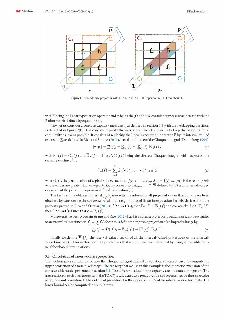
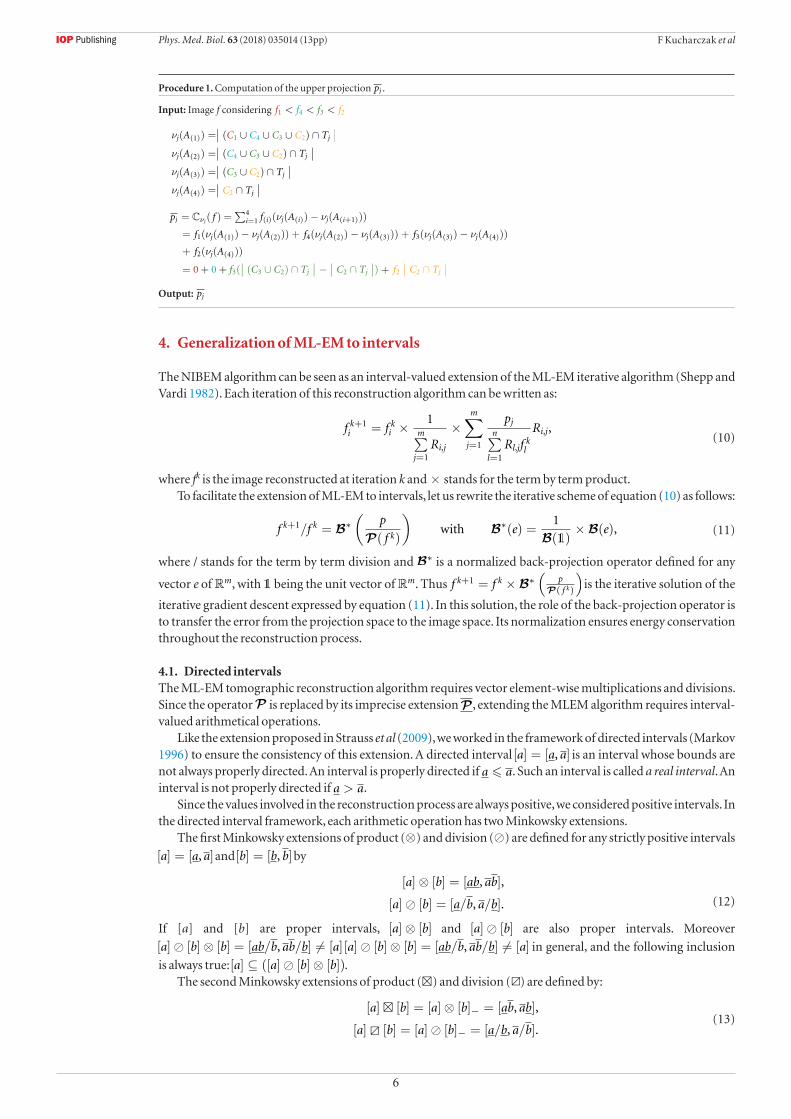
3.3. Calculation of a non-additive projectionThis section gives an example of how the Choquet integral defined by equation (8) can be used to compute the upper projection of a four-pixel image. The capacity that we use in this example is the imprecise extension of the concave disk model presented in section 3.1. The different values of the capacity are illustrated in figure 4. The intersection of each pixel group with the TOR Tj is calculated as a pseudo-code and represented by the same color in figure 4 and procedure 1. The output of procedure 1 is the upper bound pj of the interval-valued estimate. The lower bound can be computed in a similar way.

(a) (b)

Figure 4. Non-additive projection with f1 < f4 < f3 < f2. (a) Upper bound. (b) Lower bound.

Phys. Med. Biol. 63 (2018) 035014 (13pp)

6

F Kucharczak et al

4. Generalization of ML-EM to intervals

The NIBEM algorithm can be seen as an interval-valued extension of the ML-EM iterative algorithm (Shepp and Vardi 1982). Each iteration of this reconstruction algorithm can be written as:

f k+1i = f k

i × 1m∑

j=1Ri,j

×m∑

j=1

pjn∑

l=1Rl,jf k

l

Ri,j, (10)

where fk is the image reconstructed at iteration k and × stands for the term by term product.To facilitate the extension of ML-EM to intervals, let us rewrite the iterative scheme of equation (10) as follows:

f k+1/f k = B∗(

p

P( f k)

)with B∗(e) =

1

B(1)×B(e), (11)

where / stands for the term by term division and B∗ is a normalized back-projection operator defined for any

vector e of Rm, with 1 being the unit vector of Rm. Thus f k+1 = f k ×B∗(

pP( f k)

) is the iterative solution of the

iterative gradient descent expressed by equation (11). In this solution, the role of the back-projection operator is to transfer the error from the projection space to the image space. Its normalization ensures energy conservation throughout the reconstruction process.

4.1. Directed intervalsThe ML-EM tomographic reconstruction algorithm requires vector element-wise multiplications and divisions. Since the operator P is replaced by its imprecise extension P , extending the MLEM algorithm requires interval-valued arithmetical operations.

Like the extension proposed in Strauss et al (2009), we worked in the framework of directed intervals (Markov 1996) to ensure the consistency of this extension. A directed interval [a] = [a, a] is an interval whose bounds are not always properly directed. An interval is properly directed if a a. Such an interval is called a real interval. An interval is not properly directed if a > a.

Since the values involved in the reconstruction process are always positive, we considered positive intervals. In the directed interval framework, each arithmetic operation has two Minkowsky extensions.

The first Minkowsky extensions of product (⊗) and division () are defined for any strictly positive intervals

[a] = [a, a] and [b] = [b, b] by

[a]⊗ [b] = [ab, ab],

[a] [b] = [a/b, a/b].

(12)

If [a] and [b] are proper intervals, [a]⊗ [b] and [a] [b] are also proper intervals. Moreover

[a] [b]⊗ [b] = [ab/b, ab/b] = [a] [a] [b]⊗ [b] = [ab/b, ab/b] = [a] in general, and the following inclusion

is always true: [a] ⊆ ([a] [b]⊗ [b]).The second Minkowsky extensions of product () and division () are defined by:

[a] [b] = [a]⊗ [b]− = [ab, ab],

[a] [b] = [a] [b]− = [a/b, a/b]. (13)

Procedure 1. Computation of the upper projection pj .

Input: Image f considering f1 < f4 < f3 < f2

  νj(A(1)) =∣∣ (C1 ∪ C4 ∪ C3 ∪ C2) ∩ Tj

∣∣  νj(A(2)) =

∣∣ (C4 ∪ C3 ∪ C2) ∩ Tj

∣∣  νj(A(3)) =

∣∣ (C3 ∪ C2) ∩ Tj

∣∣  νj(A(4)) =

∣∣ C2 ∩ Tj

∣∣

  pj = Cνj( f ) = ∑4

i=1 f(i)(νj(A(i))− νj(A(i+1)))

    = f1(νj(A(1))− νj(A(2))) + f4(νj(A(2))− νj(A(3))) + f3(νj(A(3))− νj(A(4)))

    + f2(νj(A(4)))

    = 0 + 0 + f3(∣∣ (C3 ∪ C2) ∩ Tj

∣∣ − ∣∣ C2 ∩ Tj

∣∣) + f2

∣∣ C2 ∩ Tj

∣∣

Output: pj

Phys. Med. Biol. 63 (2018) 035014 (13pp)

7

F Kucharczak et al

Those operators are built to be the dual operators of the first extensions. We have: [a] [b] [b] = [a] and [a]⊗ [b] [b] = [a]. Those operators do not fit in the real interval framework since, if [a] and [b] are proper intervals, [a] [b] and [a] [b] are not always proper intervals.

Thus, in the directed interval framework, the following interval-valued equations:

[x]⊗ [a] = [b], (14)

[x] [a] = [b], (15)

where [a] and [b] are given and [x] is the unknown, always have a solution:

[x] [a] = [b] =⇒ [x] = [b] [a],

[x]⊗ [a] = [b] =⇒ [x] = [b] [a]. (16)

Interpreting those solutions is not straightforward. In the positive real interval framework, let [a] and [b] be two positive real intervals and let us consider the solution of equation (14). If [x] = [b] [a] is proper, then ∀a ∈ [a], ∃b ∈ [b], ∀x ∈ [x] such that a.x = b. If [x] is improper, then ∃a ∈ [a], ∀b ∈ [b], ∀x ∈ [x]− such that a.x = b, [x]− is the dual of [x] defined by [x]− = [x, x]. When [x] is proper [x]− is improper and vice versa. These semantics were formalized in Gardenes et al (2001). All those Minkowsky extensions of product and division can easily be extended to interval-valued vectors like any other arithmetic operators (see e.g. Strauss and Rico (2012)).

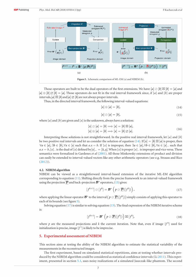
4.2. NIBEM algorithmNIBEM can be viewed as a straightforward interval-based extension of the iterative ML-EM algorithm corresponding to equation (11). Shifting directly from the precise framework to an interval-valued framework using the projection P and back-projection B∗ operators, (15) gives:

[ f k+1] [ f k] = B∗(

p P([ f k]))

, (17)

where applying the linear operator B∗ to the interval (

p P([ f k])) simply consists of applying this operator to

each of its bounds (see figure 5).Solving equation (17) is similar to solving equation (15). The final expression of the NIBEM iterative scheme

is:

[ f k+1] = B∗(

p P([ f k])) [ f k], (18)

where p are the measured projections and k the current iteration. Note that, even if image [f 0] used for initialization is precise, image [f 1] is likely to be imprecise.

5. Experimental assessment of NIBEM

This section aims at testing the ability of the NIBEM algorithm to estimate the statistical variability of the measurements in the reconstructed images.

The first experiment, based on simulated statistical repetitions, aims at testing whether intervals pro-duced by the NIBEM algorithm could be considered as statistical confidence intervals (Li 2011). This exper-iment, presented in section 5.1, uses noisy realizations of a simulated Jaszczak-like phantom. The second

(a) (b)

Figure 5. Schematic comparison of ML-EM (a) and NIBEM (b).

Phys. Med. Biol. 63 (2018) 035014 (13pp)

8

F Kucharczak et al

experiment, presented in section 5.2, aims at comparing the interval-based statistical estimation produced by NIBEM to the one relying on the bootstrap approach described in Buvat (2002). Finally, the third experi-ment, presented in section 5.4, aims at investigating the estimated uncertainty as a function of the number of counts.

5.1. NIBEM intervals as confidence intervals5.1.1. Simulation setupA modified Jaszczak-like phantom with a similar setup like that used in Li (2011) was used. It consisted of a 2D uniform disk of diameter 160 mm including six hot regions with diameters of 9.5, 11.1, 12.7, 15.9, 19.1 and 25.4 mm. The hot region concentration was 3-fold greater than the concentration of the background. The phantom was digitalized into a 64 × 64 image with 3.125 mm pixel size. The sinograms were simulated with 64 linearly sampled detector bins and 64 angular views evenly spaced over 180. The Radon matrix was computed using the rectangular MM model, implemented as described in Fessler (1995). Photon attenuation and scatter were not simulated. Three different noise levels (high, medium and low) were simulated using a Poisson random generator on noise-free projections (50 k, 250 k and 1250 k expected events in the projection data). Typical lower, upper, interval length reconstructed images and vertical profile through NIBEM reconstruction are presented in figure 6.

5.1.2. Data analysisWe performed NIBEM reconstructions of q = 1000 simulations for the three noise levels. For each pixel i, we computed how many times the true activity Ai was included in the rth estimated interval [ f r

i ] corresponding to pixel

i. The Confidence Level (CL) of the interval corresponding to the ith pixel is defined by: CLi =1q

q∑r=1

1[f ri ,f r

i ](Ai).

The mean CL of a region (hot regions or background) is estimated by averaging the CL of all pixels belonging to it.

5.1.3. ResultsTable 1 shows the mean CL of all interval-valued activity in each of the two considered regions (background and hot spots). CL of the background and the hot regions was close to 0.9. Whatever the noise level, the confidence level did not depend on the reconstructed value or on the level of noise. This experiment showed that the

reconstructed intervals could be considered as having the same CL.

5.2. NIBEM intervals as a statistical variability estimatorThis experiment aimed at testing whether the information contained in the interval-valued images reconstructed by the NIBEM algorithm could be considered as a statistical variability estimator or not. The NIBEM image statistical properties were compared with those obtained using the bootstrap approach (Buvat 2002).

Figure 6. (a) Vertical profile through the NIBEM reconstruction and ground truth, (b) lower, (c) upper, and (d) interval length (difference between the interval upper bound and lower bound) images at iteration 25 for 50k expected events in the projection data.

Phys. Med. Biol. 63 (2018) 035014 (13pp)

9

F Kucharczak et al

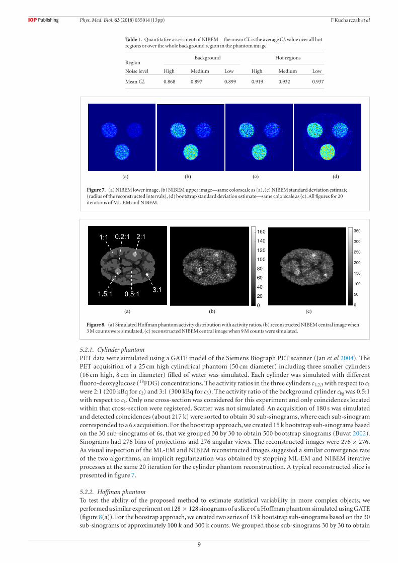
5.2.1. Cylinder phantomPET data were simulated using a GATE model of the Siemens Biograph PET scanner (Jan et al 2004). The PET acquisition of a 25 cm high cylindrical phantom (50 cm diameter) including three smaller cylinders (16 cm high, 8 cm in diameter) filled of water was simulated. Each cylinder was simulated with different fluoro-deoxyglucose (18FDG) concentrations. The activity ratios in the three cylinders c1,2,3 with respect to c1 were 2:1 (200 kBq for c2) and 3:1 (300 kBq for c3). The activity ratio of the background cylinder cbg was 0.5:1 with respect to c1. Only one cross-section was considered for this experiment and only coincidences located within that cross-section were registered. Scatter was not simulated. An acquisition of 180 s was simulated and detected coincidences (about 217 k) were sorted to obtain 30 sub-sinograms, where each sub-sinogram corresponded to a 6 s acquisition. For the boostrap approach, we created 15 k bootstrap sub-sinograms based on the 30 sub-sinograms of 6s, that we grouped 30 by 30 to obtain 500 bootstrap sinograms (Buvat 2002). Sinograms had 276 bins of projections and 276 angular views. The reconstructed images were 276 × 276. As visual inspection of the ML-EM and NIBEM reconstructed images suggested a similar convergence rate of the two algorithms, an implicit regularization was obtained by stopping ML-EM and NIBEM iterative processes at the same 20 iteration for the cylinder phantom reconstruction. A typical reconstructed slice is presented in figure 7.

5.2.2. Hoffman phantomTo test the ability of the proposed method to estimate statistical variability in more complex objects, we performed a similar experiment on 128 × 128 sinograms of a slice of a Hoffman phantom simulated using GATE (figure 8(a)). For the boostrap approach, we created two series of 15 k bootstrap sub-sinograms based on the 30 sub-sinograms of approximately 100 k and 300 k counts. We grouped those sub-sinograms 30 by 30 to obtain

(a) (b) (c) (d)

Figure 7. (a) NIBEM lower image, (b) NIBEM upper image—same colorscale as (a), (c) NIBEM standard deviation estimate (radius of the reconstructed intervals), (d) bootstrap standard deviation estimate—same colorscale as (c). All figures for 20 iterations of ML-EM and NIBEM.

(a) (b) (c)

Figure 8. (a) Simulated Hoffman phantom activity distribution with activity ratios, (b) reconstructed NIBEM central image when 3 M counts were simulated, (c) reconstructed NIBEM central image when 9 M counts were simulated.

Table 1. Quantitative assessment of NIBEM—the mean CL is the average CL value over all hot regions or over the whole background region in the phantom image.

RegionBackground Hot regions

Noise level High Medium Low High Medium Low

Mean CL 0.868 0.897 0.899 0.919 0.932 0.937

Phys. Med. Biol. 63 (2018) 035014 (13pp)

10

F Kucharczak et al

500 bootstrap sinograms (Buvat 2002) for each count level (respectively 3 M and 9 M counts). Acquisitions were pre-corrected for attenuation, normalization, scatter and random. We performed 120 iterations for NIBEM and ML-EM reconstructions. Activity ratios and typical reconstructed images of the Hoffman phantom for 3 M and 9 M counts are presented in figure 8.

5.2.3. Results

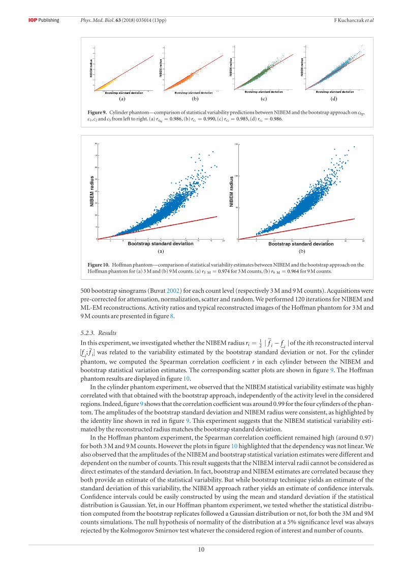
In this experiment, we investigated whether the NIBEM radius ri =12 | f i − f

i| of the ith reconstructed interval

[fi; f i] was related to the variability estimated by the bootstrap standard deviation or not. For the cylinder

phantom, we computed the Spearman correlation coefficient r in each cylinder between the NIBEM and bootstrap statistical variation estimates. The corresponding scatter plots are shown in figure 9. The Hoffman phantom results are displayed in figure 10.

In the cylinder phantom experiment, we observed that the NIBEM statistical variability estimate was highly correlated with that obtained with the bootstrap approach, independently of the activity level in the considered regions. Indeed, figure 9 shows that the correlation coefficient was around 0.99 for the four cylinders of the phan-tom. The amplitudes of the bootstrap standard deviation and NIBEM radius were consistent, as highlighted by the identity line shown in red in figure 9. This experiment suggests that the NIBEM statistical variability esti-mated by the reconstructed radius matches the bootstrap standard deviation.

In the Hoffman phantom experiment, the Spearman correlation coefficient remained high (around 0.97) for both 3 M and 9 M counts. However the plots in figure 10 highlighted that the dependency was not linear. We also observed that the amplitudes of the NIBEM and bootstrap statistical variation estimates were different and dependent on the number of counts. This result suggests that the NIBEM interval radii cannot be considered as direct estimates of the standard deviation. In fact, bootstrap and NIBEM estimates are correlated because they both provide an estimate of the statistical variability. But while bootstrap technique yields an estimate of the standard deviation of this variability, the NIBEM approach rather yields an estimate of confidence intervals. Confidence intervals could be easily constructed by using the mean and standard deviation if the statistical distribution is Gaussian. Yet, in our Hoffman phantom experiment, we tested whether the statistical distribu-tion computed from the bootstrap replicates followed a Gaussian distribution or not, for both the 3M and 9M counts simulations. The null hypothesis of normality of the distribution at a 5% significance level was always rejected by the Kolmogorov Smirnov test whatever the considered region of interest and number of counts.

Figure 9. Cylinder phantom—comparison of statistical variability predictions between NIBEM and the bootstrap approach on cbg, c1, c2 and c3 from left to right. (a) rcbg

= 0.986, (b) rc1 = 0.990, (c) rc2 = 0.985, (d) rc3 = 0.986.

Figure 10. Hoffman phantom—comparison of statistical variability estimates between NIBEM and the bootstrap approach on the Hoffman phantom for (a) 3 M and (b) 9 M counts. (a) r3 M = 0.974 for 3 M counts, (b) r9 M = 0.964 for 9 M counts.

Phys. Med. Biol. 63 (2018) 035014 (13pp)

11

F Kucharczak et al

Both information items—NIBEM confidence intervals and bootstrap standard deviations—can potentially lead to more reliable comparisons between regions of interest, and thus to more reliable diagnosis based on this comparison. But while the bootstrap approach requires generation of 15k sub-sinograms in order to make 500 bootstrap sinograms, the algorithmic complexity of the NIBEM approach is comparable to that of the MLEM approach. For example, a bootstrap reconstruction using 120 iterations of an MLEM algorithm lasted 1989 s, while, with the same setup and the same number of iterations, the NIBEM algorithm lasted only 18.4 s. i.e. 100 times faster7. Note also that the NIBEM computation time could still be reduced by paralleling some opera-tions. In addition, as NIBEM is an extension of ML-EM, an accelerated ordered subset version of NIBEM can be straightforwardly deduced from OSEM (Hudson and Larkin 2002). Preliminary tests (results not shown) showed that the ordered subset NIBEM reconstructions had properties very similar to those of NIBEM in terms of computation time and statistical variability estimation.

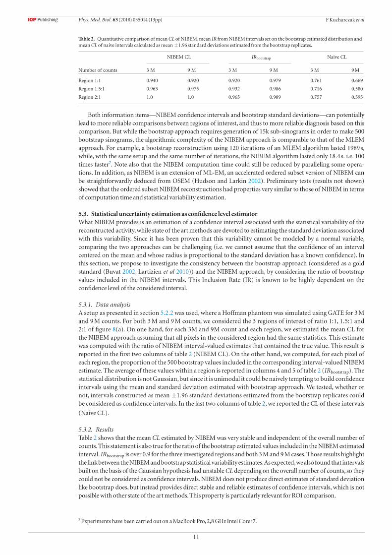
5.3. Statistical uncertainty estimation as confidence level estimatorWhat NIBEM provides is an estimation of a confidence interval associated with the statistical variability of the reconstructed activity, while state of the art methods are devoted to estimating the standard deviation associated with this variability. Since it has been proven that this variability cannot be modeled by a normal variable, comparing the two approaches can be challenging (i.e. we cannot assume that the confidence of an interval centered on the mean and whose radius is proportional to the standard deviation has a known confidence). In this section, we propose to investigate the consistency between the bootstrap approach (considered as a gold standard (Buvat 2002, Lartizien et al 2010)) and the NIBEM approach, by considering the ratio of bootstrap values included in the NIBEM intervals. This Inclusion Rate (IR) is known to be highly dependent on the confidence level of the considered interval.

5.3.1. Data analysisA setup as presented in section 5.2.2 was used, where a Hoffman phantom was simulated using GATE for 3 M and 9 M counts. For both 3 M and 9 M counts, we considered the 3 regions of interest of ratio 1:1, 1.5:1 and 2:1 of figure 8(a). On one hand, for each 3M and 9M count and each region, we estimated the mean CL for the NIBEM approach assuming that all pixels in the considered region had the same statistics. This estimate was computed with the ratio of NIBEM interval-valued estimates that contained the true value. This result is reported in the first two columns of table 2 (NIBEM CL). On the other hand, we computed, for each pixel of each region, the proportion of the 500 bootstrap values included in the corresponding interval-valued NIBEM estimate. The average of these values within a region is reported in columns 4 and 5 of table 2 (IRbootstrap). The statistical distribution is not Gaussian, but since it is unimodal it could be naively tempting to build confidence intervals using the mean and standard deviation estimated with bootstrap approach. We tested, whether or not, intervals constructed as mean ±1.96 standard deviations estimated from the bootstrap replicates could be considered as confidence intervals. In the last two columns of table 2, we reported the CL of these intervals

(Naive CL).

5.3.2. ResultsTable 2 shows that the mean CL estimated by NIBEM was very stable and independent of the overall number of counts. This statement is also true for the ratio of the bootstrap estimated values included in the NIBEM estimated interval. IRbootstrap is over 0.9 for the three investigated regions and both 3 M and 9 M cases. Those results highlight the link between the NIBEM and bootstrap statistical variability estimates. As expected, we also found that intervals built on the basis of the Gaussian hypothesis had unstable CL depending on the overall number of counts, so they could not be considered as confidence intervals. NIBEM does not produce direct estimates of standard deviation like bootstrap does, but instead provides direct stable and reliable estimates of confidence intervals, which is not possible with other state of the art methods. This property is particularly relevant for ROI comparison.

Table 2. Quantitative comparison of mean CL of NIBEM, mean IR from NIBEM intervals set on the bootstrap estimated distribution and mean CL of naive intervals calculated as mean ±1.96 standard deviations estimated from the bootstrap replicates.

NIBEM CL IRbootstrap Naive CL

Number of counts 3 M 9 M 3 M 9 M 3 M 9 M

Region 1:1 0.940 0.920 0.920 0.979 0.761 0.669

Region 1.5:1 0.963 0.975 0.932 0.986 0.716 0.580

Region 2:1 1.0 1.0 0.965 0.989 0.757 0.595

7 Experiments have been carried out on a MacBook Pro, 2,8 GHz Intel Core i7.

Phys. Med. Biol. 63 (2018) 035014 (13pp)

12

F Kucharczak et al

5.4. Estimated statistical variability as a function of the number of countsThis experiment illustrates the behavior of NIBEM confidence intervals for different number of counts.

5.4.1. Experimental setupWe simulated 100 acquisitions of the Hoffman phantom presented in figure 8(a) using GATE. Simulations corresponding to different number of counts were performed, from 100 k to 10 M with a step of 100 k counts between each. The simulated data were pre-corrected for attenuation, normalization, scatter and random. Sinograms had 128 bins of projections and 128 angular views. Reconstructions of 128 × 128 images were performed using 120 iterations of NIBEM.

5.4.2. Data analysisFigure 11(a) plots the mean NIBEM central value versus the number of counts and figure 11(b) plots the average NIBEM radius versus the numbers of counts, both for the region with a 1.5:1 activity ratio. Figure 11(c) plots the mean CL in 3 regions with 1:1, 1.5:1 and 2:1 activity ratios versus the number of counts.

5.4.3. ResultsFigure 11(a) suggests that the mean central value in the 1.5:1 region increased linearly with the number of counts. Figure 11(b) suggests that the mean NIBEM statistical variation estimate (radius) follows the same trend. Figure 11(c) highlights the fact that the NIBEM reconstructed intervals estimated stable and reliable confidence intervals for the 3 investigated regions. However, figure 11(c)) shows that if the number of counts (i.e. the signal-to-noise ratio) is high enough (approximately 1 M here), then the mean CL remains stable and higher than 90%, whatever the activity level and size of the ROI in the object.

6. Discussion

We have proposed here a new original reconstruction algorithm for Positron Emission Tomography. NIBEM is an adaption of the widely used iterative reconstruction algorithm ML-EM based on a directed interval arithmetic. One of its specificities lies in the fact that the projection operator used is interval-valued because it is based on a non-additive aggregation operator.

The main advantages of reconstructing interval-valued instead of precise activity values concern the prop-erties of the reconstructed intervals. Indeed, we showed that the radius of these intervals can be used as a statisti-cal variation predictor. In other words, it is now possible to replace the high number of statistical repetitions of ML-EM needed to estimate the reconstruction uncertainty by only one NIBEM reconstruction. The simula-tions also suggest that the reconstructed intervals might be interpreted as confidence intervals associated with the true value of the activity of each pixel. It is also important to underline that the presented method only focuses on providing an estimate of the statistical uncertainty. However, if uncertainties associated with, for instance, injected activity, scanner sensitivity, patient physiology, scatter estimate, can be quantified, they could also be integrated in the proposed framework. NIBEM is also fully compatible with time-of-flight (ToF) frame-work (Lewellen 1998). This would result in a reduction in the estimated uncertainty represented by the interval lengths.

NIBEM has a potential scope of applications in patient monitoring in oncology and in neurodegenerative disease early diagnosis. Indeed, comparing two image values at two different times, or comparing the recon-structed activities of two ROI in the same image would be greatly facilitated by the availability of confidence interval associated with each reconstructed voxel value, combined with a procedure for comparing intervals.

Figure 11. (a) Mean NIBEM central value in the 1.5:1 region as a function of the simulated number of counts, (b) radius of the NIBEM reconstructed interval in the 1.5:1 region as a function of the simulated number of counts, (c) mean CL in the 1:1, 1.5:1 and 2:1 regions.

Phys. Med. Biol. 63 (2018) 035014 (13pp)

13

F Kucharczak et al

Such procedures have already been proposed in the relevant literature (Perolat et al 2015, Denœux et al 2005). Further studies are now necessary to thoroughly investigate the behavior of reconstructed intervals provided by NIBEM, to develop appropriate statistical tests in order to decide whether two sets of intervals measured in two different ROI are different, and to model effects beyond noise and image discretization in the NIBEM framework.

Acknowledgment

This work was partially supported by the INSERM Physicancer 2012 STIPPI project and Siemens Healthineers. The authors would like to kindly thank Fayçal Ben Bouallegue for his help on the simulations, and the anonymous reviewers for their careful and meticulous reading that helped us improve this paper.

References

Barrett H, Wilson D and Tsui B 1994a Noise properties of the EM algorithm: I. Theory Phys. Med. Biol. 39 833–46Barrett H, Wilson D and Tsui B 1994b Noise properties of the EM algorithm: II. Monte Carlo simulations Phys. Med. Biol. 39 847–71Buvat I 2002 A non-parametric bootstrap approach for analyzing the statistical properties of SPECT and PET images Phys. Med. Biol.

47 1761–75Dahlbom M 2002 Estimation of image noise in PET using the bootstrap method IEEE Trans. Med. Imag. 49 2062–6Denneberg D 1994 Non-Additive Measure and Integral (Dordrecht: Kluwer) (https://doi.org/10.1007/978-94-017-2434-0)Denœux T, Massonand M and Hébert P 2005 Nonparametric rank-based statistics and significance tests for fuzzy data Fuzzy Sets Syst.

153 1–28Fessler J 1995 Aspire 3.0 user’s guide: a sparse iterative reconstruction library Technical Report 293 Department EECS, University of

Michigan, Ann ArborFessler J 1996 Mean and variance of implicitly defined biased estimators (such as penalized maximum likelihood): applications to

tomography IEEE Trans. Image Process. 5 493–506Gardenes E, Sainz M, Jorba I, Calm R, Estela R, Mielgo H and Trepat A 2001 Modal intervals Reliable Comput. 7 77–111Higdon D, Bowsher J, Johnson V, Turkington T, Gilland D and Jaszczak R 1997 Fully bayesian estimation of gibbs hyperparameters for

emission computed tomography data IEEE Trans. Image Process. 16 516–26Hudson H and Larkin R 2002 Accelerated image reconstruction using ordered subsets of projection data IEEE Trans. Med. Imaging 13 601–9Huesman R H, Gullberg G T, Greenberg W L and Budinger T F 1977 RECBL Library Users Manual: Donner Algorithms for Reconstruction

Tomography (Berkeley: Lawrence Berkeley Laboratory)Jan S et al 2004 GATE: a simulation toolkit for PET and SPECT Phys. Med. Biol. 49 4543–61Lartizien C, Aubin J and Buvat I 2010 Comparison of bootstrap resampling methods for 3D PET imaging IEEE Trans. Med. Imaging

29 1442–54Lewellen T 1998 Time-of-flight PET Semin. Nucl. Med. 28 268–75Li Y 2011 Noise propagation for iterative penalized-likelihood image reconstruction based on Fisher information Phys. Med. Biol.

56 1083–103Loquin K, Strauss O and Crouzet J 2010 Possibilistic signal processing: how to handle noise? Int. J. Approx. Reason. 51 1129–44Loquin K, Strauss O, Mariano-Goulart D and Buvat I 2014 A non-additive interval-valued reconstruction method in emission tomography

J. Nucl. Med. 55 270Markov S 1996 On directed interval arithmetic and its applications J. Universal Comput. Sci. pp 514–26Perolat J, Couso I, Loquin K and Strauss O 2015 Generalizing the Wilcoxon rank-sum test for interval data Int. J. Approx. Reason. 56 108–21Qi J and Leahy R 2000 Resolution and noise properties of MAP reconstruction for fully 3D PET IEEE Trans. Med. Imaging 19 493–506Rico A and Strauss O 2010 Imprecise expectations for imprecise linear filtering Int. J. Approx. Reason. 51 933–47Rico A, Strauss O and Mariano-Goulart D 2009 Choquet integrals as projection operators for quantified tomographic reconstruction Fuzzy

Sets Syst. 160 198–211Schmeidler D 1986 Integral representation without additivity Proc. AMS 97 255–61Shepp L and Vardi Y 1982 Maximum likelihood reconstruction for emission tomography IEEE Trans. Med. Imaging 1 113–22Sitek A 2008 Representation of photon limited data in emission tomography using origin ensembles Phys. Med. Biol. 53 3201–16Sitek A 2012 Data analysis in emission tomography using emission-count posteriors Phys. Med. Biol. 57 6779–95Soares E, Byrne C and Glick S 2000 Noise characterization of block-iterative reconstruction algorithms: I. Theory IEEE Trans. Med. Imaging

19 261–70Soares E, Glick S and Hoppin J 2005 Noise characterization of block-iterative reconstruction algorithms: II. Monte Carlo simulations IEEE

Trans. Med. Imaging 24 112–21Stayman J and Fessler J 2004 Efficient calculation of resolution and covariance for penalized-likelihood reconstruction in full 3D SPECT

IEEE Trans. Med. Imaging 23 1543–56Strauss O, Lahrech A, Rico A, Mariano-Goulart D and Telle B 2009 NIBART: A new interval based algebraic reconstruction technique for

error quantification of emission tomography images Int. Conf. Medical Image Computing and Computer-Assisted Intervention (Berlin: Springer) pp 148–55

Strauss O and Rico A 2012 Toward interval-based non-additive deconvolution in signal processing Soft Comput. 16 809–20Unser M, Aldroubi A and Eden M 1993 B-spline signal processing: part I—theory IEEE Trans. Signal Process. 41 821–33Wernick M N and Aarsvold J N 2004 The Fundamentals of PET and SPECT (Elsevier: Academic)

Phys. Med. Biol. 63 (2018) 035014 (13pp)