INTERTEMPORAL DISTURBANCES - Federal Reserve Bank of New York · in particular –nd that...

INTERTEMPORAL DISTURBANCES

GIORGIO E. PRIMICERI, ERNST SCHAUMBURG, AND ANDREA TAMBALOTTI

Abstract. Disturbances a¤ecting agents� intertemporal substitution

are the key driving force of macroeconomic �uctuations. We reach this

conclusion exploiting the bond pricing implications of an estimated gen-

eral equilibrium model of the U.S. business cycle with a rich set of real

and nominal frictions.

1. Introduction

Macroeconomic models imply two broad classes of optimization condi-

tions. On the one hand, intratemporal �rst order conditions equate the

marginal rate of substitution (MRS) between two goods consumed at the

same time to their relative price and, through this, to the marginal rate of

transformation (MRT). On the other hand, intertemporal �rst order con-

ditions equate the MRS of the same good across time to the relative price

and to the MRT.

In a stochastic general equilibrium, macroeconomic �uctuations originate

from shocks hitting these equilibrium conditions. We refer to the shocks

Date : First draft: October 2005. This version: April 2006.We thank Larry Christiano and Mark Gertler for many useful conversations, our dis-cussants Marc Giannoni, Massimiliano Pisani, Ricardo Reis and Andrea Ra¤o for theirinsightful comments, and seminar participants at the Federal Reserve Banks of Chicagoand New York, Northwestern University, Humboldt University Berlin, the 2005 SED An-nual Meeting, the Cleveland Fed conference on �Empirical Methods and Applications forDSGE and Factor Models,�the �New York Area Workshop on Monetary Policy,�the �IVWorkshop on Dynamic Macroeconomics�and the �Macroeconomic System Meeting.�Weare especially grateful to Alejandro Justiniano for many discussions on this and relatedprojects and for sharing his codes for the estimation of DSGE models. The views ex-pressed in this paper are those of the authors and do not necessarily re�ect the positionof the Federal Reserve Bank of New York or the Federal Reserve System.

1

INTERTEMPORAL DISTURBANCES 2

that directly perturb the intratemporal �rst order conditions as intratempo-

ral disturbances. This distinguishes them from intertemporal disturbances,

which perturb instead the agents�intertemporal �rst order conditions.1

This distinction is useful to state clearly the main result of this paper: in-

tertemporal disturbances are the key source of macroeconomic �uctuations.

This �nding is quite surprising, at least if considered through the lens

of some prominent work in macroeconomics. The Real Business Cycle lit-

erature, for example, has been extremely succesful in demonstrating that

economic �uctuations can be largely accounted for by neutral shifts in the

production function (Prescott (1986), King and Rebelo (1999)).2 Similarly,

Hall (1997) found that most of the movements in employment over the busi-

ness cycle are due to intratemporal �preference�shocks. These results have

been con�rmed and extended by Mulligan (2002b), Mulligan (2002c) and

Chari, Kehoe, and McGrattan (2005). Chari, Kehoe, and McGrattan (2005)

in particular �nd that intertemporal shocks� investment wedges in their ac-

counting taxonomy� are a negligible source of business cycle �uctuations.

This is true in an unconditional sense, for the entire postwar period, as well

as more speci�cally when accounting for the Great Depression and the 1982

recession.

What is the source of the discrepancy between our results and those in this

literature? We argue that the conclusion that intertemporal disturbances are

unimportant stems from the common practice of disregarding asset market

data in macroeconomics. In fact, the studies mentioned above share one

important characteristic: they concentrate on economies in which capital is

the only asset. As a consequence, their equilibrium conditions include only

one intertemporal Euler equation, that for the optimal choice of capital.

With only one Euler equation, only one intertemporal �residual�(or wedge)

1 This distinction is not necessarily a partition. Some shocks can perturb both theintratemporal and the intertemporal �rst order conditions.

2 We classify neutral technology shocks as intratemporal disturbances, because theydirectly perturb the contemporaneous relation between inputs and output. However, thischoice of label is inconsequential for the substantive results of the paper regarding thesources of business cycle �uctuations.


is identi�ed in this economy. The results in the literature suggest that this

wedge is small.

In contrast to this literature, we consider an economy in which a short-

term nominal bond is traded along with physical capital. In this economy,

the equilibrium conditions include two Euler equations, derived from the

optimal choice of each of the two assets. The key point is that with two

Euler equations we can identify two separate intertemporal disturbances,

as long as we include the short-term interest rate among the observables.

We model the �rst disturbance as a shock to the stochastic discount factor,

which captures exogenous �uctuations in preferences, as well as unmodelled

distortions in consumption choices. The second disturbance is a shock to

the rate of return on capital, which might be caused for example by changes

in the e¢ ciency of the investment technology.

We �nd that both disturbances contribute substantially to �uctuations,

even if the contribution of the combined wedge is negligible in models with

only one intertemporal Euler equation. Intuitively, large exogenous varia-

tions in the stochastic discount factor are necessary to repair the very poor

bond pricing performance of the standard Euler equation. Unfortunately

though, the resulting discount factor does not price the capital stock cor-

rectly. Hence the need for large �uctuations in the disturbance to the rate

of return.

This is not the �rst work in macroeconomics to emphasize the importance

of intertemporal shocks as sources of business cycles. Fisher (2005) identi�es

a sizable contribution to �uctuations of an investment speci�c technology

shock, one of the intertemporal shocks we include in our model, in the

context of a structural VAR. Greenwood, Hercowitz, and Krusell (2000)

show that such a shock could explain about a third of output �uctuations

in a calibrated real business cycle model, while Greenwood, Hercowitz, and

Krusell (1997) emphasize its role as a contributor to long-run growth. All

these studies use direct observations on the relative price of investment as

a proxy for the investment speci�c technological shock. On the contrary,

we measure the contribution of intertemporal disturbances to �uctuations


indirectly, as the shocks needed to reconcile the Euler equations for bonds

and capital with data on quantities and interest rates. In this respect, the

paper closest to ours is Justiniano and Primiceri (2005), who work with a

very similar model, but focus on explaining the decline in volatility of U.S.

GDP.

Our �ndings are consistent with a long line of research in �nance, dating

back at least to Hansen and Singleton�s (1982 and 1983) seminal studies

on the estimation of consumption Euler equations.3 This literature had

varying degrees of success in recovering �reasonable�estimates of taste pa-

rameters. For example, Eichenbaum, Hansen, and Singleton (1988) and

Mankiw, Rotemberg, and Summers (1985) reach opposite conclusions about

the implications of their parameter estimates for the plausibility of the im-

plied utility function. However, one result is remarkably robust across all

these studies. The overidentifying restrictions embedded in the Euler equa-

tion are consistently and overwhelmingly rejected. In other words, the Euler

equation errors are statistically large.

Our work is in line with this result, but extends it in one important

direction. As in the �nance literature, we document the size of the statistical

errors in the model�s Euler equations. In addition, by embedding these �rst

order conditions into a general equilibrium framework, we can measure the

economic importance of the disturbances in terms of their contribution to

�uctuations. We �nd that intertemporal disturbances account for a large

portion of the variation in U.S. output, consumption, investment and hours.

One possible reaction to this �nding is simply to de-emphasize the pric-

ing implications of macro models, and focus instead on their success with

quantities. This approach is well established in macroeconomics, and has

proved fruitful in addressing many interesting questions. However, we �nd it

unsatisfactory, for at least two reasons. First, in a decentralized equilibrium,

3 See Singleton (1990) for a survey of the early literature and Hall (1988) for a moremacroeconomic approach to the same issue. Campbell (2003) provides a more recentrendition of the same results, as well as an extension to several countries.


prices are the signals that lead agents to align marginal rates of substitu-

tion and transformation. Models that achieve the correct alignment of those

rates, but with the wrong prices, should at least be �puzzling.�Trying to

solve this puzzle is a challenge squarely within the realm of macroeconomics,

as forcefully argued by Cochrane (2005).4 Second, disregarding asset prices

is not a viable approach, if we are interested in modeling the short-term

nominal interest rate as the main instrument of monetary policy, as in the

modern New Keynesian literature (Woodford (2003), Smets and Wouters

(2003a), Christiano, Eichenbaum, and Evans (2005))

The paper is organized as follows. Section 2 presents the intuition behind

our results, in the context of a stylized model. Section 3 introduces a more

realistic model of the U.S. business cycle, with a rich set of nominal and

real frictions. Section 4 and 5 present the estimation results for the baseline

model and for several restricted versions of this model. Section 6 concludes.

2. The Importance of Intertemporal Disturbances

This section presents a stylized general equilibrium model, which is helpful

in illustrating the intuition behind our main results.

Consider the problem of a representative household maximizing the famil-

iar utility function, which depends on consumption (C) and hours worked

(L):

Et

1Xs=0

�sbt+s

"C1��t+s

1� � �L1+�t+s

1 + �

#.

In this formulation, bt is an exogenous shock to the consumer�s impatience,

which a¤ects both the marginal utility of consumption and the marginal

disutility of labor. The household owns the �rms and the capital stock.

Therefore, its budget constraint is given by

Ct + Tt + It +Bt � (1 + rt�1)Bt�1 +�t + wtLt + rktKt,

where Tt represents lump-sum tax payments, It is investment, Bt is the

household�s holdings of government bonds, rt is the risk-free real interest

4 A possible solution to the �puzzle� lies in the observation that prices might not beallocative. This is plausible in the case of wages, much less so in reference to asset prices.


rate, �t is the pro�t earned from owning the �rms and wt is the real wage.

Capital, denoted by Kt, is rented to �rms at the rate rkt . Households accu-

mulate the capital stock according to the equation

Kt+1 = (1� �)Kt + �tIt,

where � denotes the capital depreciation rate. �t is an investment speci�c

technology shock, a random disturbance to the e¢ ciency with which con-

sumption goods are transformed into capital, as in Greenwood, Hercowitz,

and Krusell (1997) or Fisher (2005). Therefore, in a competitive equilibrium,

��1t is equal to the relative price of investment.

In this economy, �rms operate a Cobb-Douglas production function in

capital and hours. They maximize pro�ts, taking prices as given. We close

the model with a Government, which �nances its budget de�cit by issuing

the short term bonds held by households.

Focusing on the intertemporal �rst order conditions of the consumer prob-

lem, we have

1 = Et [Mt+1 (1 + rt)](2.1)

1 = Et

�Mt+1�t

�rkt+1 +

1� ��t+1

��;(2.2)

with

Mt+1 � ��Ct+1Ct

�� bt+1bt:

Equations (2.1) and (2.2) can be interpreted as pricing equations for the

risk-free bond and the capital stock respectively. Mt+1 is the model�s sto-

chastic discount factor, which �uctuates endogenously with consumption,

and exogenously with the taste disturbance bt: The investment speci�c shock

�t; on the other hand, acts as a disturbance to the rate of return on capital.

Both disturbances perturb the model�s Euler equations. Therefore, we clas-

sify them as intertemporal disturbances. Our surprising �nding is that these

two shocks together are responsible for a large fraction of macroeconomic

�uctuations in the Unites States.

Why are our results on the importance of these intertemporal disturbances

so di¤erent from those in most of the macroeconomic literature? Because


most of that literature ignores equation (2.1) and its empirical implications.

For example, in Chari, Kehoe, and McGrattan�s (2005) prototype econ-

omy, capital is the only asset. Therefore, equation (2.1) is redundant in the

characterization of the equilibrium allocation. Moreover, markets are com-

petitive, so that the rental rate in equation (2.2) can be substituted with the

marginal product of capital. These restrictions have two important conse-

quences. First, with only one Euler equation, it is possible to identify only

one intertemporal wedge, a combination of the intertemporal disturbances

bt and �t. Second, this wedge is likely to be small, since equation (2.2) has

the best chance of �tting the data when the rental rate is measured by the

marginal product of capital (Mulligan (2002a) and Mulligan (2004)).

Why does the explicit consideration of equation (2.1) make such a dra-

matic di¤erence? Because this equation �ts the data very poorly when the

rate of return is measured on asset markets, either as a stock return or as an

interest rate on bonds (Hansen and Singleton (1982), Hansen and Singleton

(1983), Hall (1988) and Campbell (2003)). This lack of �t means that the

discrepancy between the discounted rate of return and one is statistically

large. Therefore, a large taste shock bt is necessary to reconcile the observed

market returns with the growth rate of consumption. This is true even un-

der much more general speci�cations for Mt+1 than the one adopted here

(Eichenbaum, Hansen, and Singleton (1988)). In fact, equation (2.1) is re-

soundingly rejected by tests of overidentifying restrictions, no matter what

the utility speci�cation, the measure of returns, the list of instruments, or

the frequency of the observations (see Singleton (1990) for a survey.)

Figure 1 illustrates this argument quite e¤ectively. It compares the growth

rate of consumption with measures of the marginal product of capital and

of the short-term real interest rate. Although consumption growth is more

volatile than the marginal product of capital at high frequency, the two series

clearly comove over the business cycle. The real interest rate, on the other

hand, is signi�cantly more volatile than consumption growth, especially in

the second half of the sample, and there is hardly any comovement. Given


this picture, signi�cant di¤erences in �t between equations (2.1) and (2.2)

should not be surprising.

In summary, looking at Euler equations (2.1) and (2.2) jointly, rather

than at (2.2) alone, leads to very di¤erent conclusions about the statisti-

cal size and the economic importance of intertemporal disturbances. The

model�s discount factor can price short-term bonds correctly only thanks to

exogenous movements in bt. But then, this same discount factor is unlikely

to also price the capital stock, which was instead priced reasonably well by

consumption growth alone. Hence the importance of the other intertemporal

shock, �t, to realign the return on capital with the discount factor needed

to �t equation (2.1).

But is it important to distinguish the contributions of the two intertem-

poral disturbances to �uctuations? We think the answer is yes, at least in

a world with frictions. In an e¢ cient economy, �t and bt do not play eco-

nomically independent roles. They both induce substitution of current con-

sumption with investment, and therefore future consumption� �t by mak-

ing investment cheaper, bt by making consumers more patient. Therefore,

in such an economy, a unique intertemporal wedge e¤ectively summarizes

their e¤ect. Not so in an economy with frictions, in which di¤erent shocks

will in general propagate through di¤erent mechanisms. Therefore, if we

wish to identify the sources of business cycles we need to model explicitly

the frictions that propagate them.

Of course, modeling frictions explicitly has also some drawbacks, in par-

ticular because the identi�cation of the shocks relies crucially on the exact

speci�cation of those frictions. This is why Bayesian estimation is particu-

larly suitable in this context, since it allows an explicit formal comparison

of the �t of models with alternative sets of frictions.

The aim of this section was to provide some intuition for our �ndings on

the role of intertemporal shocks in economic �uctuations. The rest of the

paper supplies the quantitative underpinnings of the arguments developed


here, in the context of an estimated DSGE model with a rich set of fric-

tions. We present this baseline model in section 3 and 4. Then, in section

5, we study the e¤ect of various restrictions on the model�s variance decom-

position. In particular, we show that in the baseline model intertemporal

shocks explain the bulk of macroeconomic �uctuations, only if we include

the short-term interest rate among the observables and equation (2.1) among

the constraints. Moreover, this result depends crucially on the inclusion of

the nominal and real frictions that our estimation procedure suggests are

important in �tting the data. In fact, the role of intertemporal shocks is

negligible in a version of the model restricted to resemble a prototypical

stochastic growth model. On the other hand, intertemporal shocks become

paramount again in a small monetary model with no investment, in which

output is equal to consumption and thus equation (2.1) is the only Euler

equation.

3. A model of the US business cycle

This section outlines our baseline model of the U.S. business cycle. This is

a medium-scale DSGE model, with a host of nominal and real frictions, along

the lines of Christiano, Eichenbaum, and Evans (2005). An important fea-

ture of this model is that its �t to U.S. data has been shown to be competitive

with that of Bayesian vector autoregressions (Smets and Wouters (2003b)

and Del Negro, Schorfheide, Smets, and Wouters (2004)). As Smets and

Wouters (2003a) and Del Negro, Schorfheide, Smets, and Wouters (2004),

we estimate this model with Bayesian methods, and use it to document the

quantitative importance of the qualitative insights discussed in section 2.

Moreover, in section 5 we consider several carefully restricted versions of

the baseline model, to highlight the source of the di¤erences between our

results and those in the literature.

The model is populated by �ve classes of agents. Producers of �nal goods,

which �assemble�a continuum of intermediate goods produced by monop-

olistic intermediate goods producers. Households, who consume the �nal


good, accumulate capital, and supply di¤erentiated labor services to compet-

itive �employment agencies�. A Government. We present their optimization

problems in turn.

3.1. Final goods producers. At every point in time t, perfectly compet-

itive �rms produce the �nal consumption good Yt, combining a continuum

of intermediate goods Yt(i), i 2 [0; 1] according to the technology

Yt =

�Z 1

0Yt(i)

11+�p;t di

�1+�p;t.

�p;t follows the exogenous stochastic process

log �p;t = (1� �p) log �p + �p log �p;t�1 + "p;t,

where "p;t is i:i:d:N(0; �2p). Pro�t maximization and the zero pro�t condition

imply the following relationship between the price of the �nal good, Pt, and

the prices of the intermediate goods, Pt(i)

Pt =

�Z 1

0Pt(i)

1�p;t di

��p;t,

and the demand function for the intermediate good i

Yt(i) =

�Pt(i)

Pt

�� 1+�p;t�p;t

Yt.

3.2. Intermediate goods producers. A monopolist produces the inter-

mediate good i according to the production function

Yt(i) = max�A1��t Kt(i)

�Lt(i)1�� AtF ; 0

,

where Kt(i) and Lt(i) denote the capital and labor inputs for the production

of good i and F represents a �xed cost of production. At is an exogenous

stochastic process capturing the e¤ects of technology, whose growth rate

(zt � � logAt) evolves according to

zt = (1� �z) + �zzt�1 + "z;t,

where "z;t is i:i:d:N(0; �2z). Therefore, the level of technology is non station-

ary.


As in Calvo (1983), a fraction �p of �rms cannot re-optimize their prices

and, therefore, set their prices following the indexation rule

Pt(i) = Pt�1(i)��pt�1�

1��p ,

where �t � PtPt�1

and � denotes the steady state value of �t. On the

other hand, re-optimizing �rms choose their price, ~Pt(i), by maximizing

the present value of future pro�ts, subject to the usual cost minimization

condition,

Et

1Xs=0

�sp�s�t+s

nh~Pt(i)

��sj=0�

�pt�1+j�

1��p�iYt+s(i)�

hWtLt(i) + r

ktKt(i)

io,

where �t+s is the marginal utility of consumption, and Wt and rkt denote

the nominal wage and the rental rate of capital.

3.3. Employment Agencies. Firms are owned by a continuum of house-

holds, indexed by j 2 [0; 1]. As in Erceg, Henderson, and Levin (2000),

each household is a monopolistic supplier of specialized labor, Lt(j): A large

number of �employment agencies�combines this specialized labor into labor

services available to the intermediate �rms, according to

Lt =

�Z 1

0Lt(j)

11+�w dj

�1+�w.

Pro�t maximization and the zero pro�t condition for the perfectly competi-

tive employment agencies imply the following relationship between the wage

paid by the intermediate �rms and the wage received by the supplier of labor

of type j; Wt(j)

Wt =

�Z 1

0Wt(j)

1�w dj

��w,

and the labor demand function

Lt(j) =

�Wt(j)

Wt

�� 1+�w�w

Lt.


3.4. Households. Each household maximizes the utility function

Et

1Xs=0

�sbt+s

�log (Ct+s � hCt+s�1)� 't+s

Lt+s(j)1+�

1 + �

�,

where Ct is consumption and h is the �degree� of habit formation.5 't is

a preference shock that a¤ects the marginal disutility of labor, while bt is a

�discount factor�shock a¤ecting both the marginal utility of consumption

and the marginal disutility of labor. These two shocks follow the stochastic

processes

log bt = �b log bt�1 + "b;t

log't = (1� �') log'+ �' log't�1 + "';t.

Note that we work with log utility to ensure the existence of a balanced

growth path, as in the real business cycle tradition. Moreover, consumption

is not indexed by j because the existence of state contingent securities en-

sures that in equilibrium consumption and asset holdings are the same for

all households.

The household�s budget constraint is

PtCt+PtIt+Bt � Rt�1Bt�1+Qt�1(j)+�t+Wt(j)Lt(j)+rkt ut

�Kt�1�Pta(ut) �Kt�1,

where It is investment, Bt is holdings of government bonds, Rt is the gross

nominal interest rate, Qt(j) is the net cash �ow from participating in state

contingent securities, and �t is the per-capita pro�t accruing to households

from ownership of the �rms.

Households own capital and choose the capital utilization rate, ut; which

transforms physical capital into e¤ective capital according to

Kt = ut �Kt�1.

E¤ective capital is then rented to �rms at the rate rkt . The cost of capital

utilization is a(ut) per unit of physical capital. As in Altig, Christiano,

5 We assume a cashless limit economy as described in Woodford (2003).


Eichenbaum, and Linde (2005), we assume that ut = 1 and a(ut) = 0 in

steady state. The physical capital accumulation equation is

�Kt = (1� �) �Kt�1 + �t�1� S

�ItIt�1

��It,

where � denotes the depreciation rate. The function S captures the presence

of adjustment costs in investment, as in Christiano, Eichenbaum, and Evans

(2005) and Altig, Christiano, Eichenbaum, and Linde (2005). We assume

that S0 = 0 and S00 > 0 in steady state.6 �t is an investment speci�c

technological shock a¤ecting the e¢ ciency with which consumption goods

are transformed into capital. In equilibrium, �t can be interpreted as the

inverse of the relative price of investment. We assume that it follows the

exogenous process

log�t = �� log�t�1 + "�;t,

where "�;t is i:i:d:N(0; �2�):

As in Erceg, Henderson, and Levin (2000), a fraction �w of households

cannot re-optimize their wages and, therefore, set them according to the

indexation rule

Wt(j) =Wt�1(j) (�t�1ezt�1)�w (�e )1��w .

The remaining fraction of re-optimizing households maximizes instead

Et

1Xs=0

�sw�sbt+s

��'t+s

Lt+s(j)1+�

1 + �

�,

subject to the labor demand function.

3.5. Government. Monetary policy sets short term nominal interest rates

following a Taylor type rule of the form

RtR=

�Rt�1R

��R "��t�

�� Yt=AtY=A

��Y #1��Re"MP;t ,

where R is the steady state for the nominal interest rate and "MP;t is an

i:i:d:N(0; �2R) monetary policy shock.

6 Lucca (2005) shows that this formulation of the adjustment cost function is equivalent(up to �rst order) to a generalization of time to build.


Fiscal policy is fully Ricardian: the Government �nances its budget de�cit

by issuing short term bonds. Public spending is determined exogenously as

a time-varying fraction of GDP

Gt =

�1� 1

gt

�Yt,

where gt is a disturbance following the stochastic process

log gt = (1� �g) log g + �g log gt�1 + "g;t.

3.6. Market Clearing. The aggregate resource constraint is

Ct + It +Gt + a(ut) �Kt�1 = Yt.

3.7. Steady State and Model Solution. In this model, consumption,

investment, capital, real wages and output evolve along a stochastic balanced

growth path, since the technology process At has a unit root. Therefore,

we �rst rewrite the model in terms of detrended variables, compute the

non-stochastic steady state of the transformed model, and then loglinearly

approximate it around this steady state.

Finally, we estimate the approximated model using as observables the

vector of variables

(3.1) [� log Yt;� logCt;� log It; logLt;� logWt

Pt; �t; Rt],

where � logXt � logXt� logXt�1. A description of the data series used inthe estimation can be found in appendix A.

3.8. Bayesian inference and priors. We use Bayesian methods to char-

acterize the posterior distribution of the structural parameters of the model

(see An and Schorfheide (2005) for a survey). As in most of the litera-

ture, we assume that the model�s exogenous disturbances are independent.

This assumption is in contrast with that adopted by Chari, Kehoe, and Mc-

Grattan (2005), whose shocks are instead allowed to be correlated. Clearly,

our assumption imposes additional restrictions on the model. On the other

hand, independence is necessary for a meaningful structural interpretation

of the shocks.


The parameters�posterior distribution combines the likelihood and the

prior information. In the rest of this subsection we brie�y discuss the as-

sumptions about the prior.

First, we �x a small number of parameters to values commonly used in

the literature. In particular, we set the steady state share of capital income

(�) to 0:33, the quarterly depreciation rate of capital, �, to 0:025 and the

steady state government spending to GDP ratio, 1 � 1=g, to 0:22, whichcorresponds to the average value of Gt=Yt in our sample.

Table 1 reports the priors for the remaining parameters of the model.

These priors are relatively disperse and are broadly in line with those adopted

in previous studies (Altig, Christiano, Eichenbaum, and Linde (2005), Del

Negro, Schorfheide, Smets, and Wouters (2004) or Levin, Onatski, Williams,

and Williams (2005)). We discuss the posterior estimates of the parameters

in the next section.

4. Empirical results for the baseline model

This section reports parameter estimates and the variance decomposition

for the baseline model of section 3. Here and in what follows we use the

fraction of the variance of the observables explained by each shock as a

measure of the shock�s contribution to �uctuations. Our objective is to

establish the importance of intertemporal disturbances as sources of those

�uctuations.

Table 2 presents posterior medians, standard deviations and 90 percent

posterior intervals for the estimated coe¢ cients of the baseline model. The

estimates are reasonable and in line with values obtained by previous studies

(Altig, Christiano, Eichenbaum, and Linde (2005), Del Negro, Schorfheide,

Smets, and Wouters (2004), Levin, Onatski, Williams, and Williams (2005),

Justiniano and Primiceri (2005)).

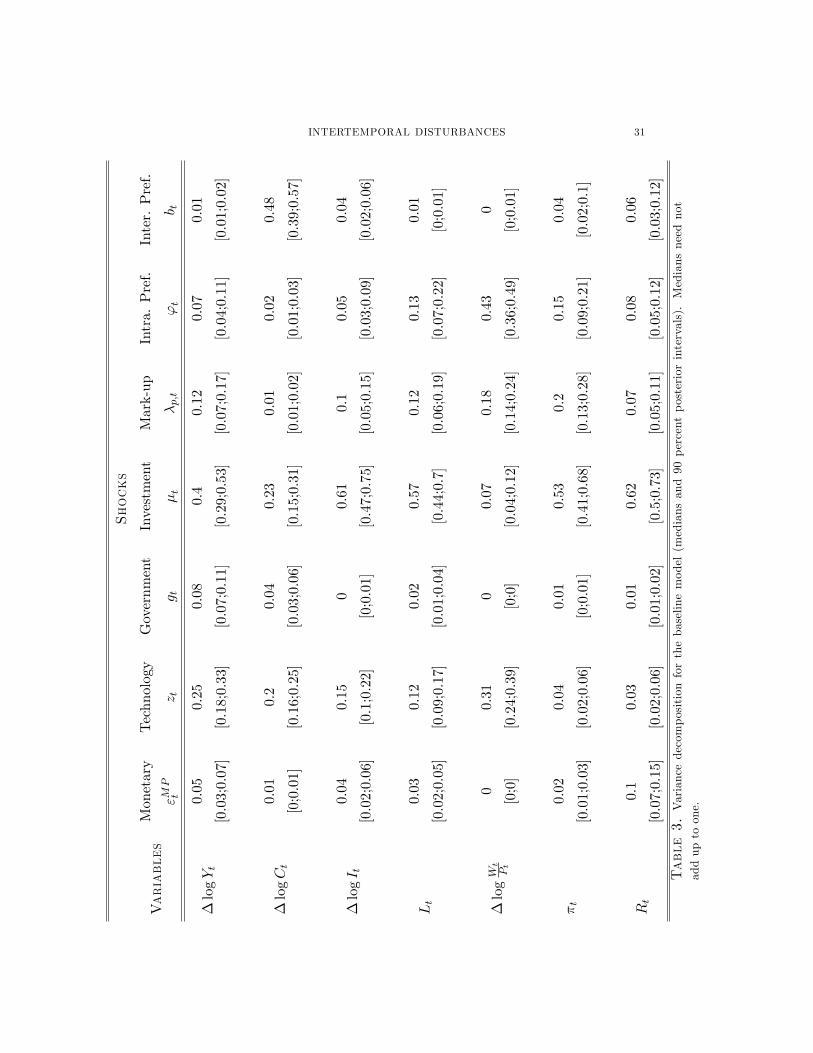
Table 3 reports the variance decomposition for the baseline model. Two

points deserve particular attention.

First, the disturbance to the stochastic discount factor is the most impor-

tant shock in explaining consumption �uctuations. The bt shock accounts


alone for almost 50 percent of the variance of consumption growth. Its

important role might be surprising, given that the baseline model features

habit formation in consumption. In fact, habits should help explain the

observed persistence in consumption, thus mitigating the empirical failure

of the Euler equation. However, the introduction of habits is also associ-

ated with high variability of the risk-free rate, as observed for example by

Boldrin, Christiano, and Fisher (2001) and Campbell and Cochrane (1999).

This might contribute to explain the importance of bt in our framework.

The second important observation from Table 3 is that the investment

speci�c technology shock �t, another intertemporal disturbance, is by far

the most important source of �uctuations in investment, as well as hours

and output. This disturbance explains about 60 percent of the variability

of investment growth, 57 percent of the variability of hours worked and

40 percent of the variability of output growth. Neutral technology shocks

account only for one forth of the variance of GDP growth and 12 and 15

percent of the variance of hours and investment growth respectively. Finally,

monetary policy shocks play a negligible role in generating �uctuations.

They account for only 5 percent of the variance of GDP.

In summary, the empirical evidence from the baseline model clearly points

to the crucial role of intertemporal disturbances in business cycle �uctua-

tions, since they account for a very large portion of the variation in consump-

tion, investment, output and hours. This �nding is very consistent with the

results in Greenwood, Hercowitz, and Krusell (2000), Fisher (2005) and Jus-

tiniano and Primiceri (2005) and broadly in line with some recent work that

has dehemphasized the role of neutral technology as a source of business

cycles (Gali (1999), Christiano, Eichenbaum, and Vigfusson (2004), Francis

and Ramey (2005a and b)).

On the contrary, the importance of intertemporal disturbances, espe-

cially as sources of �uctuations in hour, is at odds with the results of Hall

(1997), who attributes almost all those �uctuations to intratemporal prefer-

ence shocks ('t). However, in Hall (1997), as well as in Chari, Kehoe, and

McGrattan (2005), who reach similar conclusions, the intratemporal wedge


can be extracted directly, as a function of the model�s observables (and some

calibrated parameters.) In our framework instead two frictions break this

link: habit formation and sticky wages. A closer inspection of their quan-

titative role reveals that habit formation is particularly important in this

respect. In fact, when habit formation is restricted to zero, the intratempo-

ral preference shock explains 77 percent of the variance of hours, a number

much closer to Hall�s (1997) �nding.

We undertake a more systematic assessment of the relative role of the

various ingredients of the model in producing the results in the next section.

5. Assessing the role of frictions

What features of the baseline model are responsible for amplifying the role

of intertemporal shocks as a source of �uctuations? In section 2 we argued

that the main di¤erence between an RBC model with wedges and our model

is the fact that the latter includes a pricing equation for the nominal bond

and observations on its interest rate. However, this is not the only di¤erence

between the two models. In fact, our baseline model includes a host of

real and nominal frictions, like sticky wages, variable capital utilization,

adjustment costs in investment and habit formation in consumption. All

these frictions modify the model�s representation of the relevant margins for

intertemporal substitution. They could therefore play an important role in

shifting the main source of �uctuations from intratemporal to intertemporal

shocks. To asses the relative contribution of di¤erent frictions to this shift,

this section compares the variance decomposition of the baseline model to

that of a prototypical real model and of two intermediate speci�cations.

5.1. A prototypical growth model. The real model we consider is the

stochastic growth core of the model of section 3. This is obtained by as-

suming perfectly �exible prices and wages, no habit in consumption, a �xed

capital utilization rate and no adjustment costs in investment. The shocks

we consider in this case are the neutral and investment speci�c technology

shocks, zt and �t; the intratemporal preference shock, 't and the govern-

ment spending shock, gt. This is similar to the speci�cation adopted by


Chari, Kehoe, and McGrattan (2005), and we follow them in including only

output, consumption, investment and hours worked as observable variables

in the estimation. The variance decomposition for this model is in table 4.

The results are in line with the macroeconomic conventional wisdom. The

�uctuations in output and hours are entirely explained by the intratempo-

ral shocks. The neutral technology shock explains 60 percent of output

variability, with the remainder almost exclusively due to the intratemporal

preference shock, which also accounts for 95 percent of �uctuations in labor,

an even more extreme result than Hall�s (1997). However, the intertem-

poral shock (�t) does play a role in generating �uctuations in investment,

and especially in consumption, even in this simple economy. This suggests

that, although the standard Euler Equation prices capital better than bonds

(Mulligan (2002a)), its �t is far from perfect perfect.7

The impulse responses in �gure 2 clarify the intuition behind this result.

In the prototypical growth model, the �uctuations in consumption and in-

vestment generated by the intertemporal shock o¤set each other, leaving no

role for this shock to explain output. This is because embodied technological

progress generates a negative conditional correlation between consumption

and investment, which leaves output almost unchanged. As a consequence,

the likelihood would rather load on other shocks to generate business cycles,

since consumption and investment are both procyclical.

5.2. The role of real frictions. Can real rigidities alone account for the

paramount role of intertemporal disturbances in the baseline model? The

answer is no, as clearly illustrated by the results in table 5. Here, we augment

the prototypical growth model described above with all the real frictions also

featured in the baseline model. They are habit in consumption, variable

capital utilization, investment adjustment costs and (real) wage rigidity.

The variance decomposition for this model is virtually identical to that

of the previous model without frictions. Mechanically, the reason for the

7 In fact, Mulligan (2002a) shows that the standard consumption Euler equation cor-rectly prices the after-tax return on capital. Our estimated intertemporal disturbancemight therefore simply re�ect the absence of taxes in our model.


similarity of the results is that the posterior estimates of the parameters

imply a small deviation from the frictionless model, with a limited degree

of habit persistence and wage stickiness, and low investment adjustment

costs. This is because the main role of rigidities is to generate a plausible

transmission mechanism for the intertemporal shocks, as we will see in more

detail below. But in a model with no bonds and only one Euler equation,

such a mechanism is unnecessary, because intertemporal shocks can still be

safely ignored when accounting for business cycles� the one Euler equation

does not need too much help from exogenous disturbances to �t the data.

We conclude that, from the vantage point of real models, intratemporal �rst

order conditions are the ones in need of more urgent work, as also suggested

by Chari, Kehoe, and McGrattan (2005).

5.3. The role of interest rates and the bond Euler equation. The

next step is then to consider a model with nominal bonds and interest rates.

We do so by adding price stickiness to the stochastic growth model, or equiv-

alently by stripping the fully-�edged model of the consumption, investment

and wage rigidities. Compared to the two real models described above,

this speci�cation has three more observables, price and wage in�ation and

nominal interest rates, and three more shocks, to monetary policy ("MPt );

the price mark-up (�p;t) and the discount factor (bt): Of these changes, the

most important for our purposes is the inclusion of the nominal interest rate

among the observables, and of the corresponding Euler equation among the

optimization conditions. This is the equation often tested, and overwhelm-

ingly rejected, in the �nance literature.

The decomposition of the sources of �uctuations in this model is presented

in table 6. Two results stand out. First, the sum of the two intertemporal

shocks now explains 82 and 61 percent of consumption and investment �uc-

tuations respectively, almost twice as much as in the simple growth model.

Moreover, 78 and 34 percent of the �uctuations in the nominal interest

rate and in�ation are due to those same shocks. Our empirical procedure

can satisfy the restrictions imposed by the two Euler equations, in a way

which is compatible with the observed evolution of the nominal interest


rate, consumption and investment, only by loading signi�cantly on both the

intertemporal shocks. This is a result of the Euler equation�s failure as a

restriction on the returns measured in �nancial markets.

The second important result emerging from table 6 is that the variability

of output and labor remains an overwhelmingly intratemporal phenome-

non. The e¤ect of the intertemporal shocks is con�ned to �uctuations in

consumption and investment, but these �uctuations still largely o¤set each

other, resulting in virtually no movement in output and hours. This is be-

cause the model�s transmission mechanism is not rich enough to propagate

the intertemporal shocks from consumption and investment to hours and

output. This propagation is achieved only with the inclusion of real fric-

tions, as illustrated by the variance decomposition for the baseline model

in table 3. Here, the intertemporal shocks together account for 41 percent

of the �uctuations in output and 58 percent of those in labor, with the

investment speci�c technology shock playing the key role.

Figure 3 illustrates the economic mechanisms underlying this result. As in

all the models, an investment speci�c shock produces an investment boom.

Without frictions, this is mostly �nanced by a reduction in consumption,

with output almost unchanged. This is clearly not a business cycle (Green-

wood, Hercowitz, and Krusell (2000) and Greenwood, Hercowitz, and Hu¤-

man (1988)). In the model with frictions, on the other hand, the investment

boom is more gradual, due to the adjustment costs, and the reduction in

consumption is kept in check by habits. At the same time, the sensitivity of

the marginal utility of income to this change in consumption is high, ampli-

fying the positive shift in labor supply. Moreover, the increase in demand

triggered by the investment boom leads �rms to hire more labor. And since

wage stickiness �attens the labor supply curve, the result is a signi�cant

increase in hours. In addition, the drop in the relative price of new capital

makes it optimal to increase the utilization rate, which further supports the

increase in output. This increase in output in turn �nances some of the in-

vestment boom, relieving the pressure on consumption, which in fact turns

positive approximately two years after the shock.


In sum, real and nominal frictions are complementary in attributing to

intertemporal shocks a paramount role as sources of �uctuations. Including

bond pricing among the criteria for judging a model�s ability to �t the data is

necessary to highlight the de�ciencies of the standard theory of intertempo-

ral substitution. These de�ciencies manifest themselves as the shocks needed

to explain investment and consumption �uctuations in the nominal model

with no real rigidities. In this model, however, the intertemporal shocks

are not viable sources of business cycle �uctuations, because they tend to

move consumption and investment in opposite directions. The real frictions

included in the baseline model reduce signi�cantly the negative comovement

between consumption and investment, contributing to the transmission of

the intertemporal shocks to the rest of the economy.

Why should we believe the conclusions drawn from the baseline model

rather than from the model without real frictions? The reason is that the

baseline model �ts the data much better. In fact, the log marginal data

densities for the two speci�cations are equal to �2031:84 and �2224:53respectively. These values imply huge posterior odds in favor of the baseline

model.

5.4. A prototypical New-Keynesian model. The last experiment we

conduct is with a prototypical New-Keynesian model. This is a model with-

out capital accumulation dynamics. We derive it as a restricted version

of the baseline model of section 3 with no investment, so that capital is

constant over time.

Although it might not provide a particularly realistic description of the

economy, this model is interesting because it is the polar opposite of the

prototypical growth model of Chari, Kehoe, and McGrattan (2005) and

section 5.1. In fact, the only intertemporal �rst order condition in our

New-Keynesian model is the bond pricing equation, while the growth model

only features the pricing equation for the capital stock. As expected, the

analysis of this model produces opposite conclusions to those reached by

Chari, Kehoe, and McGrattan (2005) and Hall (1997).


To compare our results with those in the New-Keynesian literature, we

estimate the model using only data on output, in�ation and the short-term

nominal interest rate. These observables only allow us to identify a subset

of the shocks in the baseline model: the technology (zt), monetary policy

("MPt ), mark-up (�p;t) and discount factor (bt) shocks.

As expected, the analysis of this model produces opposite conclusions

to those reached by Chari, Kehoe, and McGrattan (2005) and Hall (1997).

First, the introduction of the discount factor shock (bt) improves the model�s

�t dramatically with respect to the case without that shock. The log mar-

ginal data density equals �872:64 for the model with variable bt, while itdecreases to �914:03 for the speci�cation with a constant discount factor,implying very high posterior odds in favor of the baseline model.

Second, the shock to the stochastic discount factor explains 75 percent

of the unconditional variance of GDP growth, as shown in table 7, while

the technology and monetary policy shocks only explain 23 and 2 percent

of that variance.8

These results further corroborate our conclusion that intertemporal dis-

turbances play a crucial role in models that explicitly include a bond-pricing

equation among their constraints. This is the case, in particular, in models

of the monetary transmission mechanism in which the short-term interest

rate is the instrument of monetary policy.

6. Concluding remarks

�If asset markets are screwed up, so is the equation of mar-

ginal rate of substitution and transformation in every macro-

economic model, so are those models�predictions for quan-

tities, and so are their policy and welfare implications. As-

set markets will have a greater impact on macroeconomics if

their economic explanation fails than if it succeeds�(Cochrane

(2005), p.3).

8 A similar result on the importance of the bt shock is obtained by Justiniano andPreston (2005) in an open economy framework.


In this paper we followed Cochrane�s (2005) advice, leveraging a well-

known failure of the standard consumption Euler equation to learn some-

thing new and surprising about the underlying sources of macroeconomic

�uctuations. The conventional wisdom in macroeconomics, as expounded

for example by Hall (1997) and Chari, Kehoe, and McGrattan (2005), is

that �uctuations derive in large part from intratemporal disturbances. We

showed instead that, in an estimated state-of-the-art model of the business

cycle, intertemporal disturbances are responsible for more than 40 percent

of output �uctuations, close to 70 percent of �uctuations in consumption

and investment, and about 60 percent of �uctuations in hours worked.

The key to this surprising result is the inclusion of the pricing equation

for bonds among the model�s equilibrium conditions and of their return

among the observables. As documented by a long line of research in �nance,

this Euler equation �ts the data very poorly. In our general equilibrium

framework, this statistical statement is equivalent to the presence of large

intertemporal disturbances. We show that these disturbances are economi-

cally important, in the sense that they explain a large fraction of economic

�uctuations. Models that ignore this basic pricing implication are likely to

reach the opposite conclusion.

Appendix A. The Data

Our dataset spans a sample from 1954QIII to 2004QIV. All data are

extracted from the Haver Analytics database (series mnemonics in paren-

thesis). Following Del Negro, Schorfheide, Smets, and Wouters (2004), we

construct real GDP by diving the nominal series (GDP) by population (LF

and LH) and the GDP De�ator (JGDP). Real series for consumption and

investment are obtained in the same manner, although consumption cor-

responds only to personal consumption expenditures of non-durables (CN)

and services (CS), while investment is the sum of personal consumption

expenditures of durables (CD) and gross private domestic investment (I).

Real wages corresponds to nominal compensation per hour in the non-farm

business sector (LXNFC), divided by the GDP de�ator. We measure the


labor input by the log of hours of all persons in the non-farm business sector

(HNFBN), divided by population. The quarterly log di¤erence in the GDP

de�ator is our measure of in�ation, while for nominal interest rates we use

the e¤ective Federal Funds rate. We do not demean or detrend any series.


References

Altig, D., L. J. Christiano, M. Eichenbaum, and J. Linde (2005): �Firm-Speci�c

Capital, Nominal Rigidities and the Business Cycle,�NBER Working Paper No. 11034.

An, S., and F. Schorfheide (2005): �Bayesian Analysis of DSGE Models,� mimeo,

University of Pennsylvania.

Boldrin, M., L. J. Christiano, and J. Fisher (2001): �Habit Persistence, Asset

Returns and the Business Cycle,�American Economic Review, 91, 149�166.

Calvo, G. (1983): �Staggered Prices in a Utility-Maximizing Framework,� Journal of

Monetary Economics, 12(3), 383�98.

Campbell, J. Y. (2003): �Consumption-Based Asset Pricing,� in Handbook of the Eco-

nomics of Finance, ed. by G. Constantinides, M. Harris, and R. Stulz, vol. 1B, chap. 13,

pp. 803�887. North-Holland, Amsterdam.

Campbell, J. Y., and J. H. Cochrane (1999): �By Force of Habit: A Consumption

Based Explanation of Aggragate Stock Market Behavior,�Journal of Political Economy,

109, 1238�87.

Chari, V., P. J. Kehoe, and E. R. McGrattan (2005): �Business Cycle Accounting,�

Federal Reserve Bank of Minneapolis, Research Department Sta¤ Report 328.

Christiano, L. J., M. Eichenbaum, and C. L. Evans (2005): �Nominal Rigidities and

the Dynamic E¤ect of a Shock to Monetary Policy,�The Journal of Political Economy,

113(1), 1�45.

Christiano, L. J., M. Eichenbaum, and R. Vigfusson (2004): �What Happens After

a Technology Shock?,�mimeo, Northwestern University.

Cochrane, J. H. (2005): �Financial Markets and the Real Economy,�mimeo, University

of Chicago.

Del Negro, M., F. Schorfheide, F. Smets, and R. Wouters (2004): �On the Fit and

Forecasting Performance of New Keynesian Models,� Federal Reserve Bank of Atlanta

Working Paper No. 2004-37.

Eichenbaum, M., L. P. Hansen, and K. J. Singleton (1988): �A Time-Series Analysis

of Representative Agent Models of Consumption and Leisure Choice under Uncertainty,�

Quarterly Journal of Economics, 103, 51�78.

Erceg, C. J., D. W. Henderson, and A. T. Levin (2000): �Optimal Monetary Policy

with Staggered Wage and Price Contracts,�Journal of Monetary Economics, 46(2), 281�

313.

Fisher, J. D. M. (2005): �The Dynamic E¤ect of Neutral and Investment-Speci�c Tech-

nology Shocks,�mimeo, Federal Reserve Bank of Chicago.


Francis, N. R., and V. A. Ramey (2005a): �Is the Technology-Driven Real Busi-

ness Cycle Hypothesis Dead? Shocks and Aggregate Fluctuations Revisited,�Journal of

Monetary Economics, forthcoming.

(2005b): �Measures of Hours Per Capita and their Implications for the

Technology-Hours Debate,�University of California, San Diego, mimeo.

Gali, J. (1999): �Technology, Employment, and the Business Cycle: Do Technology

Shocks Explain Aggregate Fluctuations?,�American Economic Review, 89(1), 249�271.

Greenwood, J., Z. Hercowitz, and G. W. Huffman (1988): �Investment, Capacity

Utilization, and the Real Business Cycle,�American Economic Review, 78(3), 402�417.

Greenwood, J., Z. Hercowitz, and P. Krusell (1997): �Long Run Implications of

Investment-Speci�c Technological Change,�American Economic Review, 87(3), 342�362.

Greenwood, J., Z. Hercowitz, and P. Krusell (2000): �The role of investment-

speci�c technological change in the business cycle,�European Economic Review, 44(1),

91�115.

Hall, R. E. (1988): �Intertemporal Substitution in Consumption,� Journal of Political

Economy, 96(2), 339�357.

(1997): �Macroeconomic Fluctuations and the Allocation of Time,� Journal of

Labor Economics, 15(2), 223�250.

Hansen, L. P., and K. J. Singleton (1982): �Generalized Instrumental Variables

Estimation of Nonlinear Rational Expectations Models,�Econometrica, 50, 1269�1286.

(1983): �Stochastic Consumption, Risk Aversion, and Temporal Behavior of

Asset Returns,�Journal of Political Economy, 91, 249�268.

Justiniano, A., and B. Preston (2005): �Can Structural Small Open Economy Models

Account for the In�uence of Foreign Shocks?,�mimeo, Board of Governors of the Federal

Reserve System, Washington D.C.

Justiniano, A., and G. E. Primiceri (2005): �The Time Varying Volatility of Macro-

economic Fluctuations,�NBER Working Paper no. 12022.

King, R. G., and S. T. Rebelo (1999): �Resuscitating Real Business Cycles,�in Hand-

book of Macroeconomics, ed. by J. B. Taylor, and M. Woodford, Amsterdam. North-

Holland.

Levin, A. T., A. Onatski, J. C. Williams, and N. Williams (2005): �Monetary Policy

Under Uncertainty in Micro-Founded Macroeconometric Models,� in NBER Macroeco-

nomics Annual.

Lucca, D. O. (2005): �Resuscitating Time to Build,�mimeo, Northwestern University.

Mankiw, N. G., J. Rotemberg, and L. Summers (1985): �Intertemporal Substitution

in Macroeconomics,�Quarterly Journal of Economics, 100, 225�251.

Mulligan, C. B. (2002a): �Capital, Interest, and Aggregate Intertemporal Substitution,�

NBER working paper no. 9373.


(2002b): �A Century of Labor-Leisure Distorsion,� NBER working paper no.

8774.

(2002c): �A Dual Method of Empirically Evaluating Dynamic Competitive Equi-

librium Models with Market Distorsions, Applied to the Great Depression and World

War II,�NBER working paper no. 8775.

(2004): �Robust Aggregate Implications of Stochastic Discount Factor Volatility,�

NBER working paper no. 10210.

Prescott, E. C. (1986): �Theory Ahead of Business Cycle Measurement,�Federal Re-

serve Bank of Minneapolis Quarterly Review, 10(4), 9�22.

Singleton, K. J. (1990): �Speci�cation and Estimation of Intertemporal Asset Pricing

Models,�in Handbook of Monetary Economics, ed. by B. Friedman, and F. Hahn. North-

Holland, Amsterdam.

Smets, F., and R. Wouters (2003a): �An Estimated Stochastic Dynamic General

Equilibrium Model of the Euro Area,� Journal of the European Economic Association,

1(5), 1123�1175.

(2003b): �Shocks and Frictions in US Business Cycles: A Bayesian Approach,�

mimeo, European Central Bank.

Woodford, M. (2003): Interest and Prices: Foundations of a Theory of Monetary Policy.

Princeton University Press, Princeton, NJ.


Northwestern University and NBER

E-mail address : [email protected]

Northwestern University


Federal Reserve Bank of New York



Coefficient Density Mean StDev

�p Beta 0.5 0.15

�w Beta 0.5 0.15

Normal 0.5 0.025

h Beta 0.5 0.1

�p Normal 0.15 0.05

�w Normal 0.15 0.05

� Normal 0.5 0.1

r Normal 0.5 0.1

� Gamma 2 0.75

�p Beta 0.75 0.1

�w Beta 0.75 0.1

� Gamma 5 1

S00 Normal 4 1.5

�� Normal 1.7 0.3

�y Gamma 0.125 0.1

�R Beta 0.5 0.15

�z Beta 0.5 0.15

�g Beta 0.5 0.15

�� Beta 0.5 0.15

��p Beta 0.5 0.15

�' Beta 0.5 0.15

�b Beta 0.5 0.15

�R Inverse Gamma 0.15 0.15

�z Inverse Gamma 0.15 0.15

�g Inverse Gamma 0.15 0.15

�� Inverse Gamma 0.15 0.15

��p Inverse Gamma 0.15 0.15

�' Inverse Gamma 0.15 0.15

�b Inverse Gamma 0.15 0.15

Table 1. Prior densities for the model coe¢ cients.


Coefficient Median StDev 5th percentile 95th percentile

�p 0.165 0.067 0.081 0.296

�w 0.099 0.029 0.056 0.151

0.423 0.024 0.382 0.46

h 0.815 0.026 0.767 0.853

�p 0.241 0.038 0.178 0.304

�w 0.138 0.037 0.081 0.201

� 0.564 0.099 0.398 0.722

r 1.021 0.08 0.887 1.154

� 3.629 0.893 2.389 5.316

�p 0.779 0.023 0.739 0.817

�w 0.736 0.037 0.668 0.791

� 7.284 1.082 5.644 9.219

S00 1.728 0.491 1.142 2.725

�� 2.043 0.142 1.842 2.305

�y 0.068 0.014 0.046 0.091

�R 0.8 0.022 0.76 0.833

�z 0.321 0.055 0.233 0.413

�g 0.977 0.007 0.964 0.988

�� 0.924 0.024 0.877 0.956

��p 0.854 0.039 0.784 0.911

�' 0.494 0.07 0.372 0.607

�b 0.832 0.039 0.766 0.894

�R 0.257 0.015 0.236 0.284

�z 1.168 0.066 1.071 1.287

�g 0.643 0.04 0.581 0.71

�� 0.127 0.018 0.103 0.159

��p 0.103 0.011 0.086 0.123

�' 1.077 0.261 0.718 1.608

�b 0.569 0.139 0.399 0.856

Table 2. Posterior estimates for the coe¢ cients of the baseline model.

INTERTEMPORAL DISTURBANCES 31Shocks

Variables

Monetary

"MP

t

Technology

z t

Government

g t

Investment

�t

Mark-up

�p;t

Intra.Pref.

't

Inter.Pref.

b t

�logYt

0.05

[0.03;0.07]

0.25

[0.18;0.33]

0.08

[0.07;0.11]

0.4

[0.29;0.53]

0.12

[0.07;0.17]

0.07

[0.04;0.11]

0.01

[0.01;0.02]

�logCt

0.01

[0;0.01]

0.2

[0.16;0.25]

0.04

[0.03;0.06]

0.23

[0.15;0.31]

0.01

[0.01;0.02]

0.02

[0.01;0.03]

0.48

[0.39;0.57]

�logI t

0.04

[0.02;0.06]

0.15

[0.1;0.22]

0

[0;0.01]

0.61

[0.47;0.75]

0.1

[0.05;0.15]

0.05

[0.03;0.09]

0.04

[0.02;0.06]

Lt

0.03

[0.02;0.05]

0.12

[0.09;0.17]

0.02

[0.01;0.04]

0.57

[0.44;0.7]

0.12

[0.06;0.19]

0.13

[0.07;0.22]

0.01

[0;0.01]

�logWt

Pt

0

[0;0]

0.31

[0.24;0.39]

0

[0;0]

0.07

[0.04;0.12]

0.18

[0.14;0.24]

0.43

[0.36;0.49]

0

[0;0.01]

�t

0.02

[0.01;0.03]

0.04

[0.02;0.06]

0.01

[0;0.01]

0.53

[0.41;0.68]

0.2

[0.13;0.28]

0.15

[0.09;0.21]

0.04

[0.02;0.1]

Rt

0.1

[0.07;0.15]

0.03

[0.02;0.06]

0.01

[0.01;0.02]

0.62

[0.5;0.73]

0.07

[0.05;0.11]

0.08

[0.05;0.12]

0.06

[0.03;0.12]

Table

3.Variancedecompositionforthebaselinemodel(mediansand90percentposteriorintervals).Mediansneednot

adduptoone.


Shocks

VariablesTechnology

zt

Government

gt

Investment

�t

Intra. Pref.

't

� log Yt0.60

[0.55;0.65]

0.01

[0;0.01]

0.02

[0.01;0.03]

0.37

[0.32;0.43]

� logCt0.26

[0.22;0.31]

0.12

[0.1;0.16]

0.57

[0.52;0.62]

0.04

[0.03;0.06]

� log It0.23

[0.2;0.27]

0.24

[0.18;0.3]

0.27

[0.23;0.33]

0.25

[0.21;0.3]

Lt0.01

[0;0.02]

0.01

[0;0.01]

0.04

[0.02;0.06]

0.95

[0.91;0.97]

Table 4. Variance decomposition for the prototypical growth model(medians and 90 percent posterior intervals). Medians need not add up

to one.


Shocks

VariablesTechnology

zt

Government

gt

Investment

�t

Intra. Pref.

't

� log Yt0.61

[0.56;0.67]

0.00

[0.00;0.01]

0.04

[0.02;0.06]

0.35

[0.3;0.4]

� logCt0.15

[0.12;0.19]

0.06

[0.05;0.09]

0.75

[0.7;0.79]

0.03

[0.02;0.06]

� log It0.32

[0.27;0.37]

0.22

[0.17;0.27]

0.26

[0.21;0.31]

0.21

[0.18;0.24]

Lt0.01

[0.00;0.01]

0.01

[0.00;0.01]

0.03

[0.01;0.07]

0.95

[0.91;0.98]

Table 5. Variance decomposition for the growth model with real fric-tions (medians and 90 percent posterior intervals). Medians need not

add up to one.

INTERTEMPORAL DISTURBANCES 34Shocks

Variables

Monetary

"MP

t

Technology

z t

Government

g t

Investment

�t

Mark-up

�p;t

Intra.Pref.

't

Inter.Pref.

b t

�logYt

0.01

[0.00;0.02]

0.55

[0.49;0.6]

0.01

[0.00;0.01]

0.04

[0.02;0.06]

0.03

[0.02;0.06]

0.32

[0.27;0.37]

0.04

[0.02;0.07]

�logCt

0.00

[0.00;0.00]

0.08

[0.07;0.11]

0.06

[0.04;0.08]

0.37

[0.32;0.43]

0.01

[0.01;0.02]

0.02

[0.01;0.03]

0.45

[0.4;0.51]

�logI t

0.00

[0.00;0.01]

0.12

[0.1;0.14]

0.13

[0.08;0.18]

0.27

[0.23;0.32]

0.04

[0.02;0.05]

0.10

[0.08;0.13]

0.33

[0.28;0.39]

Lt

0.00

[0.00;0.00]

0.01

[0.00;0.01]

0.01

[0.00;0.02]

0.01

[0.01;0.03]

0.02

[0.01;0.04]

0.91

[0.83;0.96]

0.03

[0.02;0.07]

�logWt

Pt

0.13

[0.06;0.22]

0.40

[0.34;0.46]

0.00

[0.00;0.00]

0.01

[0.00;0.01]

0.38

[0.33;0.43]

0.07

[0.05;0.08]

0.01

[0.01;0.02]

�t

0.53

[0.44;0.63]

0.07

[0.05;0.09]

0.01

[0.01;0.02]

0.29

[0.23;0.34]

0.01

[0.00;0.01]

0.05

[0.02;0.11]

0.04

[0.02;0.08]

Rt

0.00

[0.00;0.00]

0.12

[0.1;0.16]

0.02

[0.02;0.03]

0.71

[0.62;0.77]

0.02

[0.01;0.02]

0.06

[0.03;0.11]

0.07

[0.03;0.12]

Table6.

Variancedecompositionforthegrowthmodelwithnominalfrictions(mediansand90percentposteriorintervals).

Mediansneednotadduptoone.


Shocks

VariablesMonetary

"MPt

Technology

zt

Mark-up

�p;t

Inter. Pref.

bt

� log Yt0.02

[0.01;0.03]

0.23

[0.14;0.38]

0.01

[0;0.02]

0.75

[0.59;0.84]

�t0

[0;0]

0

[0;0]

1

[0.99;1]

0

[0;0.01]

Rt0.12

[0.08;0.17]

0

[0;0.03]

0.4

[0.27;0.55]

0.47

[0.32;0.61]

Table 7. Variance decomposition for the prototypical New-

Keynesian model (medians and 90 percent posterior intervals). Medians

need not add up to one.

Con

sum

ptio

n G

row

th a

nd th

e R

ate

of R

etur

n

8.0

6.0

4.0

2.00.0

2.0

4.0

6.0

8.0

Q1:54 Q3:55 Q1:57 Q3:58 Q1:60 Q3:61 Q1:63 Q3:64 Q1:66 Q3:67 Q1:69 Q3:70 Q1:72 Q3:73 Q1:75 Q3:76 Q1:78 Q3:79 Q1:81 Q3:82 Q1:84 Q3:85 Q1:87 Q3:88 Q1:90 Q3:91 Q1:93 Q3:94 Q1:96 Q3:97 Q1:99 Q3:00 Q1:02 Q3:03 Q1:05

Con

sum

ptio

n G

row

thR

etur

n on

Cap

ital

Rea

l Int

eres

t Rat

e

Figure1.Consumptiongrowthisthegrowthrateofper-capitaconsumption.ThereturnoncapitalisMPKt+1��;where

MPK=�Y KisthemarginalreturnoncapitalforaCobb-Douglasproductionfunction.Theseriesforthecapitalstock(K)is

constructedfrom

thecapitalaccumulationequationusingobservationsoninvestmentandK0equaltothecapitalstock�ssteady

statevalue.The(ex-post)realinterestrateisi t��t+1;whereiistheinterestrateonthree-monthTreasuryBillsand�isthe

growthrateoftheGDPde�ator.Allvariablesareannualizedanddemeaned.Datasourcesandde�nitionsareinappendixA.

0 2 4 6 8 10 12 14 16 18 200

0.1

0.2

0.3

0.4

0.5Impulse Responses to an Investment Specific Technology Shock

outp

ut

0 2 4 6 8 10 12 14 16 18 200.8

0.6

0.4

0.2

0

0.2

cons

umpt

ion

0 2 4 6 8 10 12 14 16 18 200.8

1

1.2

1.4

1.6

inve

stm

ent

0 2 4 6 8 10 12 14 16 18 200.05

0.1

0.15

0.2

0.25

hour

s

Figure 2. Impulse responses to an investment speci�c technology shock (�t) for theprototypical growth model (medians and 90 percent posterior intervals.)

0 2 4 6 8 10 12 14 16 18 200.5

1

1.5

2

2.5

3Impulse Responses to an Investment Specific Technology Shock

outp

ut

0 2 4 6 8 10 12 14 16 18 201

0.5

0

0.5

1

1.5

cons

umpt

ion

0 2 4 6 8 10 12 14 16 18 200

2

4

6

8

inve

stm

ent

0 2 4 6 8 10 12 14 16 18 201

0

1

2

3

hour

s

Figure 3. Impulse responses to an investment speci�c technology shock (�t) for thebaseline model (medians and 90 percent posterior intervals.)

INTERTEMPORAL DISTURBANCES - Federal Reserve Bank of New York · in particular –nd that...

Documents

Transcript of INTERTEMPORAL DISTURBANCES - Federal Reserve Bank of New York · in particular –nd that...