Interrogation Systems for Fiber Bragg Grating-Based...

Interrogation Systems for Fiber Bragg Grating-Based Sensors

Maria-Iulia Comanici

Department of Electrical and Computer Engineering McGill University Montreal, Canada

June, 2010 A thesis submitted to McGill University in partial fulfilment of the requirements of the

degree of Master of Engineering

© Maria-Iulia Comanici

1

Abstract

As the potential application of fiber optic sensors broadens, there is much interest

in finding measurement systems that are simple, cost effective and show high power

efficiency. The latter is extremely useful when dealing with multiplexed sensors

distributed over large distances, which results in high signal attenuation and limits the

number of sensors that can be interrogated by a minimum number of measurement units.

In this thesis we explore a fiber laser-based wavelength-to-power mapping interrogation

system for wavelength-division-multiplexed FBG sensors, and we prove that such

solution offers increased measurement reliability with high power efficiency.

Another aspect of improving the performance of sensing systems is the ability to

measure multiple parameters, which are extremely useful when working with FBG-based

sensors experiencing similar changes in spectral characteristics in response to changes in

temperature or strain. These can be discriminated when they can be measured using

different interrogation methods. For this purpose, we first explore and evaluate the

performance of a vibration sensor designed by QPS Photronics, and we prove that it can

be used to measure temperature and/or strain by translating the changes in its sinusoidal

multi-wavelength spectrum to changes in the response of a single pass-band microwave

photonic filter (MPF). The operation principle is based on monitoring the shift of the

main filter band as temperature or strain changes. We demonstrate that such a system can

achieve high-speed measurement with variable sensitivity.

2

Abrégé

Avec la croissance de l’application potentielle des capteurs à fibres optiques, il

est important de trouver des systèmes de mesure simples, à coût réduit, et présentant une

efficacité de puissance élevée. Celle-ci est extrêmement utile quand il s’agit de

multiplexer des capteurs distribués sur des grandes distances, ce qui contribue à

l’augmentation de l’atténuation du signal optique et impose une limite au nombre de

capteurs qui peuvent être interrogés en utilisant un minimum d’unités de mesure. Dans

cette thèse nous explorons un système d’interrogation basé sur un laser à fibre optique

pour réaliser la traduction de la longueur d’onde en une mesure de puissance pour les

capteurs à base de réseaux de Bragg. Nous prouvons que grâce à cette solution nous

pouvons augmenter la fiabilité de la mesure avec une efficacité de puissance élevée ainsi

que de réduire les erreurs de la mesure.

Pour augmenter la performance d’un système de capteurs, il est aussi important de

pouvoir mesurer de paramètres additionnels. Ceci est extrêmement important quand le

capteur est base sur des réseaux de Bragg qui ont une réponse similaire aux changements

de température ou tension. Ces deux facteurs peuvent être distingués en utilisant des

méthodes d’interrogation différentes. Ainsi, nous explorons et évaluons premièrement la

performance d’un capteur de vibration conçu par QPS Photronics. Nous prouvons qu’il

est possible de mesurer aussi la température et/ou la tension en traduisant les

changements du spectre à plusieurs longueurs d’onde en des changements de la réponse

d’un filtre à micro-ondes photoniques (MPF) à une seule bande passante. Le principe de

l’opération du système est base sur la surveillance du déplacement de la bande passante

principale du filtre quand la température ou la tension de la fibre changent. Nous

montrons qu’un tel système est capable d’assurer une mesure très rapide avec une

sensibilité variable.

3

Acknowledgements

First, I thank my supervisor, Professor Lawrence Chen, for his constant dedication

at giving guidance and advice to help me improve my practical and analytical skills to

attain my research goals. It has been an honour working with you for the past two years.

Second, I am grateful for the financial support provided by the Canadian Institute

fo Photonic Innovations Technology, Exploitation, and Networking Grant with QPS

Photronics. I thank Dr. Peter Kung, the founder and director of the company, for the

additional help with providing equipment for the experiments involved in the project. I

strongly appreciate the work of the people I met at the company. They were always

available to share their expertise to help me acquire additional skills. Moreover, I am

thankful to the team at Optech, who have allowed me to use their equipment for

conducting a number of experiments at their lab.

Working within the Photonic Systems Group at McGill University has given me

the opportunity to meet amazing people. I thank them for their help and friendship. I am

grateful to Professors Andrew Kirk and Martin Rochette, who have shared their

knowledge by teaching a number of undergraduate and graduate courses. I thank Dr.

Pegah Seddighian for assisting with the project and for teaching me a number of practical

skills during these two years. I also thank Dr. Victor Torres-Company, and Dr. Chen

Chen for their availability on numerous occasions, when they helped me to either debug

problems, or to use a number of measurement instruments. I thank Dr. Joshua Schwartz

for always being available and prompt at providing me with the equipment necessary for

the experimental setup. I thank Sandrine for her assistance with writing the abstract in

French and being a great friend.

Last but not least, I am extremely grateful to my family for their always being

available when I needed help and support the most. I thank my brothers: Johnny for being

there for me, Silviu for always being cheerful, helpful, and, whenever possible, ready to

escort me to or from school when I had pressing matters to deal with; and Ghita, who has

been a great friend and always ready to give a helping hand. I also thank his fiancé

Demetra, who was a real friend. I feel blessed to have my young sister Elena, who always

succeeded at putting a smile on my face. I thank my parents Mariana and Ioan, who

4

always put their interests aside to attend to the needs of their children. My mother has

been a remarkable parent and my best friend. I am extremely grateful to my father for the

interest in my success he always showed. He taught me the valuable study skills that

helped me achieve my goals.

5

Table of Contents

List of Figures ........................................................................................... 7

List of Acronyms .................................................................................... 13

1. Introduction ........................................................................................ 14 1.1 Fiber Optic Sensing..................................................................................................................14 1.2 Characteristics of Fiber Optic Sensor Systems........................................................................14 1.3 Types of Fiber Optic Sensors ...................................................................................................15 1.4 Fiber Bragg Grating (FBG) Sensors .......................................................................................16 1.5 Motivation and Thesis Contributions ......................................................................................18 1.6 References.................................................................................................................................20

2. Fiber Bragg Gratings Background................................................... 22 2.1 Introduction ..............................................................................................................................22 2.2 Principles Behind FBGs Fabrication ......................................................................................23 2.3 Coupling Properties of FBGs...................................................................................................25

2.3.1 Non-uniform FBGs Used as Sensors .................................................................................27 2.4 Strain and Temperature Effect on FBGs ................................................................................28

2.4.1 Strain Effect on FBGs ........................................................................................................28 2.4.2 Temperature Effect on FBGs ............................................................................................29 2.4.3 FBG Temperature and Strain Sensors Interrogation .....................................................29 2.4.4 Temperature Independent Strain Sensing .......................................................................31

2.5 Summary...................................................................................................................................32 2.6 References.................................................................................................................................33

3. Fiber Bragg Grating Vibration Sensors for Condition Monitoring37 3.1 Introduction ..............................................................................................................................37 3.2 VibroFiberTM System Design....................................................................................................38

3.2.1 Operation Principle ............................................................................................................38 3.2.2 Sensor Packaging................................................................................................................40 3.2.3 Sensor Measurement System and Instrumentation.........................................................41

3.3 Sensor Test Characterization ...................................................................................................44 3.3.1 Frequency Response Measurement...................................................................................44 3.3.2 Amplitude Response Measurement...................................................................................46 3.3.3 Repeatability Test ...............................................................................................................47

3.4 Case Study ................................................................................................................................50 3.4.1 Sensor 1300-10 ....................................................................................................................50 3.4.2 Sensor 1300-19 ....................................................................................................................52 3.4.3 Sensor 1300-20 ....................................................................................................................54 3.4.4 Sensor V1300-22 .................................................................................................................56

3.5 Summary of Measurement Results ..........................................................................................58 3.6 Power Budget for TDM Applications ......................................................................................60

6

3.6.1 Objective............................................................................................................................. 60 3.6.2 Power Budget Experiment ................................................................................................ 61

3.7 Discussion and Summary ........................................................................................................ 66 3.8 References................................................................................................................................ 68

4. Microwave Photonic Filter-based Interrogation System for VibroFiberTM Sensors.............................................................................70 4.1 Introduction ............................................................................................................................. 70 4.2 Microwave Photonic Filter Background................................................................................. 71 4.3 Fiber Bragg Grating Pair Based Sensor Temperature Response .......................................... 73 4.4 Microwave Phototnic Filter-based Temperature Measurement ............................................ 78

4.4.1 Temperature Effect on the Response of a MPF .............................................................. 78 4.4.2 Effect of Delay Fiber Length on the Characteristics of the MPF .................................. 79 4.4.3 Temperature Measurement Using a MPF System .......................................................... 82

4.5 Conclusion and Discussion ..................................................................................................... 87 4.6 References................................................................................................................................ 88

5. Improved Arrayed Waveguide Grating-based Interrogation System for Fiber Bragg Grating Sensors...........................................................90 5.1 Introduction ............................................................................................................................. 90 5.2 Fiber Laser Systems................................................................................................................. 92 5.3 AWGs as Edge Filter Components.......................................................................................... 94 5.4 Experimental Setup and Measurement Method ..................................................................... 97 5.5 Experimental Results............................................................................................................. 100

5.5.1 Using an SOA as Broadband Source.............................................................................. 100 5.5.2 Using an EDFA as Broadband Source ........................................................................... 107 5.5.3 Continuous-Time Measurement Results........................................................................ 111

5.6 Discussion and Conclusion ................................................................................................... 117 5.7 References.............................................................................................................................. 119

6. Conclusion and Future Work..........................................................122

7

List of Figures

Figure 1.1: Fiber optic sensing system: a) transmission mode; b) reflection mode. ........15

Figure 2.1: Schematic for the coupling between the wave reflected off the FBG and the

input wave [2.8]. ...............................................................................................................22

Figure 2.2: Interferometric method of writhing FBGs in optical fiber’s core [2.1]..........24

Figure 2.3: Phase-mask (diffraction based) FBG writing method [2.6]. ..........................25

Figure 2.4: OSA based interrogation system for FBG strain or temperature sensors.......29

Figure 2.5: Passive interrogation system for FBGs [2.30]................................................30

Figure 3.1: Schematic for the VibroFiberTM sensor head. ................................................39

Figure 3.2: Fiber Fabry-Perot cavity reflection spectrum for different reflectivities of the

interferometer reflectors....................................................................................................39

Figure 3.3: Reflection Spectrum for a VibroFiberTM sensor.............................................39

Figure 3.4: Sensor head placement inside the protection case..........................................40

Figure 3.5: Type B package: a) Three dimensional view of the individual components; b)

Transverse view of the sensor head that is placed inside the sensor protection case. ......41

Figure 3.6: Controlled sensor test system. ........................................................................41

Figure 3.7: The method to place the sensor on the shaker plate: (a) physical, (b) pictorial.

...........................................................................................................................................42

Figure 3.8: VibroFiberTM detection system. .....................................................................42

Figure 3.9: Wavelength at which the laser is biased for the vibration measurement. ......43

Figure 3.10: User interface illustrating the measurement of the vibration signal.............44

Figure 3.11: Measured frequency response for a VibroFiberTM vibration sensor (sensor

package of type A). ...........................................................................................................45

Figure 3.12: Amplitude response plot for a vibration sensor (sensor package of type A).

...........................................................................................................................................47

Figure 3.13: Qualitative characterization of the vibration sensor measurement

repeatability (sensor package of type A): M1 to M8 represent the different measurements

recorded.............................................................................................................................48

Figure 3.14: Design for sensor 1300-10. ..........................................................................50

Figure 3. 15: Frequency response for sensor V1300-10. ..................................................51

8

Figure 3.16: Plot of the measured value as a function of vibration amplitude at frequency

100 Hz for sensor V1300-10.............................................................................................52


Figure 3.18: Frequency response for sensor V1300-19. ...................................................53

Figure 3.19: Plot of the measured value as a function of vibration amplitude at 100 Hz for

sensor V1300-19. ..............................................................................................................54


Figure 3.21: Frequency response for sensor V1300-20. ...................................................55

Figure 3.22: Plot of the measured value as a function of vibration amplitude at 100 Hz for

sensor V1300-20. ..............................................................................................................55


Figure 3.24: Frequency response for rensor V1300-22. ...................................................56

Figure 3.25: Plot of the measured value as a function of vibration amplitude at frequency

100 Hz for sensor V1300-22.............................................................................................57

Figure 3.26: Spectrum of sensor 1300-22 when the frequency is 150 Hz and the vibration

amplitude is 10 μm............................................................................................................57

Figure 3.27: Power budget measurement system. ............................................................61

Figure 3.28: The system of N cascaded sensors: continuous vertical line represents a

connector; double oblique lines represent the sensor double grating configuration. Note

that the vertical lines represent APC connectors or splices. .............................................62

Figure 3.29: Number of sensors that may be interrogated as a function of reflectivity, at

different total lengths, when the input power is 10 dBm, the sensors are connected using

splicing, and the last sensor reflectivity is 0.1. .................................................................63

Figure 3.30: Number of sensors that may be interrogated as a function of sensor

reflectivity, at different total lengths, when the input power is 10 dBm, the sensors are

connected using APC connectors, and the last sensor reflectivity is 0.1..........................63

Figure 3.31: Number of sensors that may be interrogated for two different last sensor

reflectivity values when the input power is 0 dBm, the fiber length is 10 km and the

sensors are connected using splicing. ...............................................................................64

9

Figure 3.32: Number of sensors that can be interrogated as a function of sensor

reflectivity when the input power is -9.15 dBm, the sensors are connected using splicing

over a distance of 10 km, and the last sensor reflectivity is 0.8. ......................................65

Figure 4.1: General schematic for a MPF system [4.3][4.4]. ...........................................71

Figure 4.2: Setup used to measure FBG pair spectrum change with temperature............74

Figure 4.3: FBG comparison of reflection spectra at room temperature and at a) °100 C ,

and at b) °50 C. ..................................................................................................................75

Figure 4.4: Reflection spectrum center wavelength of an FBG pair as a function of

temperature. ......................................................................................................................76

Figure 4.5: MPF response at room temperature when the single mode fiber length is 85

km. ....................................................................................................................................79

Figure 4.6: First maximum superimposed on the estimated wavelength spacing between

the filter peaks as functions of SMF fiber length..............................................................80

Figure 4.7: Experimental setup used to find the optimum SMF fiber length. ..................80

Figure 4.8: MPF response superimposed on the dispersion response of the SMF fiber of

length 85 km used as delay line. .......................................................................................81

Figure 4.9: Measured modulator transfer function over 20 GHz of RF frequency. .........81

Figure 4.10: MPF experimental setup..............................................................................82

Figure 4.11: Shift in the MPF as temperature is increased from 25 to 100 °C.................83

Figure 4.12: Graph of power measured as temperature is increased for different

modulator RF bias frequencies located on the rising edge of the second filter peak........84

Figure 4.13: Graph of power measured as temperature is increased for different

modulator RF bias frequencies located on the falling edge of the second filter peak. .....84

Figure 4.14: Graph of normalized power variation as a function of temperature when the

bias RF frequency is 8.98 GHz. ........................................................................................85

Figure 4.15: Graph of normalized power variation as a function of temperature when the

bias RF frequency is 9.24 GHz. ........................................................................................86

Figure 5.1: Principle of mapping wavelength to power using an edge filter [5.1]. ..........91

Figure 5.2: Fiber laser configurations: a) standing wave configuration; b) ring

configuration. ....................................................................................................................92

Figure 5.3: (a) AWG geometric structure; (b) Geometric representation of the FPR. .....95

10

Figure 5.4: Conventional wavelength to power mapping system.....................................98

Figure 5.5: Standing wave fiber laser system used to achieve wavelength to power

mapping.............................................................................................................................98

Figure 5.6: Ring fiber laser system used to achieve wavelength to power mapping........98

Figure 5.7: Mechanism to apply and measure strain. .......................................................99

Figure 5.8: FBG reflection spectra for the conventional wavelength to power mapping

system. ............................................................................................................................101

Figure 5.9: FBG reflection spectra for the standing wave fiber laser wavelength to power

mapping system. .............................................................................................................101

Figure 5.10: FBG reflection spectra for the ring fiber laser wavelength to power mapping

system. ............................................................................................................................102

Figure 5.11: Curve used to extract the zero strain point for the FBG whose reflection

spectrum is centered at 1538.32 nm................................................................................103

Figure 5.12: Calibration curve for the FBG whose reflection spectrum is centered at

1538.32 nm. ....................................................................................................................103

Figure 5.13: Measured power as a function of strain plot. .............................................104

Figure 5.14: Mapping curve showing the wavelength corresponding to the power level

measured for different strain levels.................................................................................105

Figure 5.15: Measured power at the output of the AWG corresponding to the FBG of

reflection spectrum center wavelength at 1538.323 nm for the three wavelength-to-power

mapping systems.............................................................................................................106

Figure 5.16: Measured normalized power at the output of the AWG corresponding to the

FBG of reflection spectrum center wavelength at 1538.32 nm for the three wavelength-

to-power mapping systems used to evaluate measurement resolution. ..........................106

Figure 5.17: In-house built EDFA for the FBG-based strain sensors interrogation

systems............................................................................................................................107

Figure 5.18: Measured power at the output of the AWG as a function of strain for the

sensor whose reflection spectrum is centered at 1538.32 nm when the in-house built

EDFA is used. .................................................................................................................108

11

Figure 5.19: Measured power at the output of the AWG as a function of strain for the

sensor whose reflection spectrum is centered at 1538.32 nm when a unidirectional EDFA

is used..............................................................................................................................108

Figure 5.20: Normalized measured power at the output of the AWG as a function of

strain for the sensor whose reflection spectrum is centered at 1538.32 nm when the in-

house built EDFA is used. ..............................................................................................109

Figure 5.21: Normalized measured power at the output of the AWG as a function of

strain for the sensor whose reflection spectrum is centered at 1538.32 nm when a

unidirectional EDFA is used...........................................................................................109

Figure 5.22: Spectral characteristic of FBG 2 when using the fiber laser configuration

when an EDFA is used as gain medium. ........................................................................110

Figure 5.23: Experimental setup for time-domain measurements using an RSOA........111

Figure 5.24: The FBG and AWG spectra when the former is placed in the ultrasonic bath

at 25 °C. ..........................................................................................................................112

Figure 5.25: Response to the ultrasonic signal when the FBG is placed in the ultrasonic

bath at 25 °C. ..................................................................................................................112

Figure 5.26: The FBG and AWG spectra when the former is placed in the ultrasonic bath

and water is heated to 50 °C. ..........................................................................................113

Figure 5.27: Response to the ultrasonic signal when the FBG is placed in the ultrasonic

bath at 50 °C. ..................................................................................................................113

Figure 5.28: DC amplitude level when the temperature is a) 25 °C, and b) 50 °C.........114

Figure 5.29: FBG wavelength as a function of applied strain. .......................................115

Figure 5.30: Measured mean amplitude measured with the oscilloscope at the output of

the AWG channel corresponding to the FBG under test as a function of applied strain.115

Figure 5.31: Wavelength-to-electric signal mean amplitude mapping when the FBG

overlaps with a) the rising, and b) the falling edges of the AWG channel. ....................116

12

List of Tables

Table 3.1: Example of measuring the operability regions for a VibroFiberTM. ...........46

Table 3.3: Quantitative characterization of the VibroFiberTM measurement repeatability.......................................................................................................................................49

Table 3.4: Sensor versions V1295 with packages of type B........................................58

Table 3.5: Sensor versions V1300 with packages of type B........................................59

Table 3.6: Sensors with packages of type A. ...............................................................59

Table 3.7: Sensor versions V1264 with packages of type A. ......................................59

Table 3.8: Sensor versions V1300 with packages of type A .......................................59

Table 3.9: Sensor versions V1280 with packages of type A. ......................................60

Table 5.1: Summary of FBG reflection spectra measured bandwidths with the associated wavelength measurement errors. ...............................................................................102

Table 5.2: Summary of FBGs sensitivities to strain. .................................................104

Table 5.3: Summary of FBG reflection spectra measured bandwidths with the associated wavelength measurement errors when an EDFA is used as BBS and as gain medium:110

13

List of Acronyms

APC Angle Polished Connector

ASE Amplified Spontaneous Emission

AWG Arrayed Waveguide Grating

BBS Broadband Source

BW Bandwidth

CW Continuous-Wave

DC Direct Current

EDFA Erbium-Doped Fiber Amplifier

EO-MZM Electro-Optic Mach-Zehnder Modulator

FBG Fiber Bragg Grating

FSR Free Spectral Range

FWHM Full Width at Half Maximum

HPS High Performance System

LCA Lightwave Component Analyzer

LD Laser Diode

LPG Long Period Grating

MPF Microwave Photonic Filter

MZM Mach-Zehnder Modulator

OSA Optical Spectrum Analyzer

RF Radio Frequency

RSOA Reflective Semiconductor Optical Amplifier

SMF Single Mode Fiber

SOA Semiconductor Optical Amplifier

TDM Time-Division-Multiplexing

TEC Thermo-Electric Controller

UV Ultraviolet

VOA Variable Optical Attenuator

WDM Wavelength-Division-Multiplexing

14

1. Introduction

1.1 Fiber Optic Sensing

Sensing plays an important role in many applications using equipment that

experiences degradation over time due to external forces or environmental factors. For

example, civil structures experience degradation by being exposed to rain and to

changing temperature. Moreover, these factors combined with exposure to external forces

lead to cracks that can cause failure. Therefore, to avoid damage, it is important to detect

and replace the equipment that experiences a certain amount of degradation, which in

many cases can be considered dangerous. In this context, it is important to have sensors

capable to detect changes in the physical or in the chemical composition of structures

accurately. With the advent of fiber optic communications, it has been observed that

using a dielectric medium to guide information in the form of light is more efficient than

using metallic media to transmit electrical signals. Besides their excellent transmission

characteristics, optical fiber sensors are attractive because they show the ability to

confine the signal so that no electro-magnetic interference is experienced—a common

issue encountered when using electrical signals: their operation requires electro-magnetic

isolation and thus adds complexity to the detection system. Moreover, optical fibers are

light and compact, which makes them useful in remote sensing and allows for packaging

flexibility.

1.2 Characteristics of Fiber Optic Sensor Systems

A sensing system is built using the components shown in Figure 1.1. As observed,

signal de-multiplexing can be achieved either in transmission or in reflection mode, as in

Figure 1.1 a) and b), respectively. The light source is either broadband or pulsed,

depending on the type of signal the sensor head is designed to process [1.1]. The optical

sensor head responds to changes in environmental conditions by modulating the signal

characteristics; these can then be detected using a photo-detector or an optical instrument

that is able to measure the signal characteristic that has been modified; this change can be

reflected in the wavelength, power, polarization, or phase of the optical signal. The

detection system can be improved by processing the signal to get the accurate

15

measurement of the parameter the information is encoded into. The performance of a

sensor system is determined by the extent to which, following calibration, a unique

processed value corresponds to a particular environmental condition. Moreover, the

sensitivity of the sensor and its measurement range play equally important roles. The

former is defined by the change in the detected signal per unit of environmental condition

change, while the latter defines the number of values that the system is able to accurately

measure. In most applications, the sensors are used in real time, and the response time

becomes an important parameter in evaluating the accuracy of the sensing system [1.1].

a)

b)

Figure 1.1: Fiber optic sensing system: a) transmission mode; b) reflection mode.

1.3 Types of Fiber Optic Sensors

Extensive studies show that optical fibers are sensitive to changes in external

environmental parameters such as temperature, strain, and pressure. The former induces a

change in refractive index which affects the guiding properties of the optical fibers. Strain

and pressure affect the geometry of the fiber and thus induce changes in the effective

refractive index, which characterizes the propagation mode area and losses.

These characteristics are reflected in the intensity or in the spectral characteristics of

the optical signal detected at the output of the fiber: external factors modulate either the

16

light’s amplitude or wavelength [1.2]. Moreover, progress in the field of fiber

interferometers allows translating changes in phase or in spectral characteristics to

changes in signal intensity. This approach extends the range of applications and the

ability to tailor the sensing characteristics. Another classification of fiber optic sensor is

based on whether the sensing region is lumped at the sensing location—point sensor—or

it is distributed along the length of the fiber—distributed sensing [1.1]. The latter takes

advantage of and explores techniques based on stimulated Brillouin scattering, stimulated

Raman scattering, or optical time-domain spectrometers [1.3].

1.4 Fiber Bragg Grating (FBG) Sensors

FBGs can be used as point sensors because they are built by writing periodic

structures resulting from the modulation of optical fibers’ core refractive index over a

short fiber length. Their spectral characteristics replicate the changes imposed on the

effective refractive index resulting by the exposure to changing strain and temperature. In

particular, FBGs reflect a narrow band of wavelengths centered about the Bragg

(resonance) wavelength, which shifts in response to the aforementioned environmental

factors. As a result, many applications aimed at monitoring strain and temperature

changes have been explored and find practical use [1.4]. Of particular interest is the

application of FBG sensors to structural health monitoring [1.5][1.6]. In this context, R.

Maaskant et al. discuss the application of surface attached FBGs to monitoring the

condition of different materials-based pre-stressed tendons, which are embedded in

concrete girders, used in the structure of the Beddington Trail Bridge in Calgary,

(Alberta, Canada) [1.5]. In the study, the strain monitoring helped researchers to identify

the long-term behaviour of different materials and the effectiveness of using a newly

proposed material— Carbon Fiber Composite Cable (CFCC). Other practical applications

to civil structures have been used in monitoring the condition of Horsetail Falls Bridge in

Oregon. In this case, the strains from twenty-six FBGs were successfully measured

[1.7][1.8]. Saouma et al. have succeeded at applying FBG-based strain measurement to

evaluate the properties of aluminum as a composite material for civil structures

[1.7][1.9]. In another study, H.L. Ho et al. propose an FBG-based sensing system capable

of detecting the static and dynamic responses of strain and temperature as applied to

17

studying the heat transfer properties of non-stationary flow and the induced vibrations.

The static detection system involves using a scanning tuneable filter whose wavelength is

tuned to the Bragg wavelength of the sensing FBGs and is placed before detecting the

reflection spectrum of the grating. After the static measurement is completed, the

dynamic measurement is achieved by setting the tuneable filter center wavelength to a

wavelength where the slope of the FBG reflection spectrum is maximum—a point where

the dynamic measurement is the most sensitive. Therefore, as dynamic strain is applied to

the system is detected from a change in the voltage signal detected at the output of the

tuneable filter [1.10]. The same principle can be also used to aerospace and civil

applications, to determine the properties of composite materials, and to monitor the effect

of static and dynamic load on electric transmission lines. An example of using a tuneable

filter based detection system is provided by V.M. Murukeshan et al. in [1.11]. In this

case, the sensor is used to monitor the cure process of composite materials, and is based

on embedded FBG sensors. Temperature measurements have also been achieved using

FBG sensors. For example, for application to civil structures, FBG temperature sensors

are packaged to achieve isolation from strain and pressure effects [1.12].

Moreover, other parameters that are related to temperature or strain can be monitored.

For example, to build a hydrophone, sound waves have the same effect strain has on

FBGs, i.e., it causes a physical change in the length of the grating, and, consequently, its

pitch. As a result of this phenomenon, the reflection wavelength shifts as it would under

the effect of strain, with the difference that, in terms of sensitivity, sound waves have the

same effect as pressure [1.13]. Recently, Y.-L. Park et al. propose embedding FBGs in

robot component structures to measure contact or grasping forces. This parameter is

measured using the information provided by changes in strain as forces are applied to

FBGs [1.14]. Furthermore, as presented by F. Xie et al., a Michelson interferometer built

using FBGs can be used to measure displacement. Here, the property that FBGs are

sensitive to temperature is used to compensate for environmental changes and thus

measure the desired parameter—displacement—only [1.15]. Another application would

be creating an acceleration sensor whose information can be converted to FBG strain

changes, as proposed by J. Chang et al in [1.16].

18

1.5 Motivation and Thesis Contributions

Today, knowledge on the propagation and physical characteristics of optical fibers

has led to the emergence of a number of applications. Even though sensing using FBG

technology is mature enough to provide the necessary tools to generate, to transmit, and

to modulate light in response to desired external parameters, the detection unit

performance is limited by the propagation properties in guiding media. Specific

limitations include the following:

• Power efficiency is limited by the losses incurred by the propagation distance, which

is relatively long in most applications, especially remote sensing.

• The decoding method deployed usually involves using expensive, often bulky, and

thus unpractical, instrumentation.

• Finally, multiplexing enhances the complexity of detection systems.

This thesis is aimed at providing simplified and less expensive solutions to decoding

the information provided by two different designs of FBG-based sensors. First, chapter

two introduces the theory behind light propagation in such structures. The chapters that

follow provide solutions to the aforementioned problems that prevent the practical use of

FBG sensors. Chapter 3 provides the characterization of a currently deployed vibration

sensing system design. Next, in Chapter 4, the possibility to map this sensor’s spectral

information to microwave photonic filter variation to measure temperature is

experimentally proven. Finally, previous studies show that using wavelength to power

mapping using edge filters can simplify the method used to measure the changes induced

when axial strain is applied to FBGs: instead of using an optical spectrum analyzer to

measure wavelength change, a power meter, which is cheaper and less bulky, can be used

to measure change in power. However, insertion losses are associated to both FBGs and

filters, and, as a result, the simplified detection method comes at the expense of high

transmission powers because this type of sensors find use in sensing over long distances.

Therefore, Chapter 5 of this thesis proves the ability to combine the partial reflectivity

and wavelength selectivity of FBGs in a fiber laser configuration to obtain improved

mapping and enhanced power efficiency, which are associated to the lasing nature of the

system. In this context, the performances of ring and of standing wave fiber laser

19

configurations will be compared and discussed. Performance will be evaluated in terms

of the ability to achieve lasing at all FBGs in the sensor array and in terms of

measurement sensitivity and power efficiency. In this contect, the received power needs

to be enhanced by at least 20 dB to satisfy the improved measurement capability over

long distances. Moreover, the ability to use different sources and fiber laser gain media

will be investigated for the purpose of reducing the overall system cost.

The studies that are presented in this thesis can also be found in the following

publications:

• M.-I. Comanici and L. R. Chen, “Improved arrayed waveguide grating-based interrogation system for fiber Bragg grating sensors,” 14th OptoElectronics and Communications Conference (OECC), 13-17 July 2009, Hong Kong, paper WQ3.

• P. Kung, M.-I. Comanici, and L.R. Chen, “Fiber Bragg grating vibration sensors for condition monitoring of hydro-electric turbine windings,” Photons, vol.7 no. 2, 2009. • M.-I. Comanici, L. R. Chen, and P. Kung, "Interrogating fiber Bragg grating sensors based on single bandpass microwave photonic filtering," International Topical Meeting on Microwave Photonics, 5 - 9 October 2010, Montreal, QC, paper FRI-5.

20

1.6 References

[1.1] W. Boyes, Instrumentation Reference Book, pp. 191-216, Ed. 4, Butterwirth-Heinemann: Burlington, MA, 2010.

[1.2] E. Udd, “Overview of Fiber Optic Sensors” in Fiber Optic Sensors, edited by S.

Yin, and P. B. Ruffin, F. T. S. Yu, ed. 2, pp. 1-34, CRC Press: Boca Raton, FL, 2008.

[1.3] A. Bueno, K. Nonaka, and S. Sales, “Hybrid interrogation system for distributed

fiber strain sensors and point temperature sensors based on pulse correlation and FBGs,” IEEE Photonics Technology Letters, vol. 21, no. 22, pp. 1671-1673, 2009.

[1.4] A. Othonos, “Fiber Bragg gratings,” Review of Scentific Instruments, vol. 68, no.

12, pp. 4309-4341, 1997. [1.5] R. Maaskant, T. Alavie, R. M. Measures, G. Tadroq, S. H. Rizkalla, and A. Guha-

Thakurta, “Fiber-optic Bragg grating sensors for bridge monitoring,” Cement and Concrete Composites, vol. 19, pp. 21-33, 1997.

[1.6] C. K. Y. Leung, “Fiber optic sensors in concrete: the future?,” NDT&E

International, vol. 34, pp. 85–94, 2001. [1.7] M. Majumder, T. K. Gangopadhyay, A. K. Chakraborty, K. Dasgupta, and D. K.

Bhattacharya, “Fibre Bragg gratings in structural health monitoring—Present status and applications,” Sensors and Actuators A, vol. 147, pp. 150–164, 2008.

[1.8] W. L. Schulz, J. P. Conte, E. Udd, and J. M. Seim, “Static and dynamic testing of

bridges and highways using long-gage fibre Bragg grating based strain sensors,” Proceedings SPIE, vol. 4202, pp. 79-86, 2000.

[1.9] V. E. Saouma, D. Z. Anderson, K. Ostrander, B. Lee, and V. Slowik,

“Application of fibre Bragg grating in local and remote infrastructure health monitoring,” Materials Structure, vol. 31, pp. 259–266, 1998.

[1.10] H. L. Ho, W. Jin, C. C. Chan, Y. Zhou, and X. W. Wang, “A fiber Bragg grating

sensor for static and dynamic measurands,” Sensors and Actustors A, vol. 96, pp. 21-24, 2002.

[1.11] V. M. Murukeshan, P. Y. Chan, L. S. Ong, and L. K. Seah, “Cure monitoring of

smart composites using fiber Bragg grating based embedded sensors,” Sensors and Actuators, vol. 79, pp. 153–161, 2000.

[1.12] P. Moyo, J. M. W. Brownjohn, R. Suresh, and S. C. Tjin, “Development of fiber

Bragg grating sensors for monitoring civil infrastructure,” Engineering Structures, vol. 27, pp. 1828–1834, 2005.

21

[1.13] N. Takahashi, K. Yoshimura, S. Takahashi, and K. Imamura, “Development of an optical fiber hydrophone with fiber Bragg grating,” Ultrasonics, vol. 38, pp. 581–585, 2000.

[1.14] Y. Park, K. Chau, R. J. Black, and M. R. Cutkosky, “Force sensing robot fingers

using embedded fiber Bragg grating sensors and shape deposition manufacturing,” 2007 IEEE International Conference on Robotics and Automation Roma, Italy, 10-14 April 2007.

[1.15] F. Xie, X. Chen, and L. Zhang, “High stability interleaved fiber Michelson

interferometer for on-line precision displacement measurements,” Optics and Lasers in Engineering, vol. 47, pp. 1301-1306, 2009.

[1.16] J. Chang, Q. Wang, X. Zhang, D. Huo, L. Ma, X. Liu, T. Liu, and C. Wang, “A

fiber Bragg grating acceleration sensor interrogated by a DFB laser diode,” Laser Physics, vol. 19, no. 1, pp. 134-137, 2009.

22

2. Fiber Bragg Gratings Background

2.1 Introduction

With the advent of optical communications, optical fiber plays an important role in

signal transmission. Also, work has been invested in fabricating in-fiber devices capable

of tailoring the properties of light so optical fibers can be used to perform other tasks,

which usually are accomplished by electronic devices and thus involve conversion losses

and limit the system’s speed. One such in-fiber structure is the FBG, whose properties

were investigated after the discovery of photosensitivity: by doping the core of a single

mode optical fiber with certain compounds, ultraviolet (UV) radiation can be absorbed

and thus induce a permanent refractive index change [2.1]. Different methods are used in

combination with the photosensitivity effect to obtain the periodic modulation of the core

refractive index, which is able, through partial reflection at each high-low and low-high

refractive index change, to reconstruct a reflected signal whose spectrum is centered at a

wavelength that satisfies the Bragg condition: Λ= nB 2λ , where Λ is the pitch of the

periodically modulated core refractive index, and n is the effective refractive index [2.2].

The structure of an FBG and its spectral characteristics are shown in Figure 2.1.

z=0 z=l

)(zEi

)(zEr

)(zEt

Figure 2.1: Schematic for the coupling between the wave reflected off the FBG and the input wave [2.8].

This chapter first describes the principle behind the writing of FBGs in the core of

optical fibers. This is followed by the presentation of the coupled mode theory behind the

23

operation of FBGs. Next, the principles behind the effect of two environmental and

physical factors, i.e., temperature and strain, are presented, followed by a discussion on

the methods used to measure and discriminate these parameters.

2.2 Principles Behind FBGs Fabrication

The photosensitivity effect was first observed in highly Ge doped fiber. However,

other methods to increase photosensitivity in single mode fibers usually used in

telecommunications include hydrogenation (hydrogen loading), flame brushing, and

boron co-doping. Hydrogenation is achieved because, under conditions of high pressure

and high temperature, hydrogen diffuses into the Ge-Si core. This method is not

permanent, so as the hydrogen concentration decreases, the strength of the

photosensitivity effect decreases. The next method is flame brushing and involves

hydrogen diffusion into the fiber core under very high temperatures (up to °1700 C). [2.3]

This is achieved by repeatedly (and for short periods of time) exposing the region to be

photosynthesized to a hydrogen-rich flame. The high temperature causes the hydrogen

diffusion. The major problem encountered when using high temperatures is the

possibility of damaging the fiber. While the aforementioned methods increase

photosensitivity through the formation of germanium-oxygen deficiency centers, boron

co-doping helps to enhance photosensitivity through photo-induced stress relaxation,

which affects the thermo-mechanical interaction between the boron doped core and the

silica cladding. This implies the accumulation of thermo-elastic stress in the core [2.3].

In the writing process, the properties of FBGs depend on the wavelength of the

ultraviolet light for photosensitivity and on the inscription method for the refractive index

distribution, which sets the resonance reflected wavelength. There are two methods of

writing FBGs into the core of an optical fiber: holographic and non-interferometric [2.1].

Holographic inscription uses interfering UV light to create the periodic pattern induced

by the photosensitive effect. A first mechanism (illustrated in Figure 2.2) to create the

interference would be to split an incoming radiation into two separate beams that

experience different optical path lengths. However, since these paths are sensitive to

external environmental conditions, this technique needs to be applied in a controlled

environment to avoid FBG inscription errors.

24

Figure 2.2: Interferometric method of writhing FBGs in optical fiber’s core [2.1].

An alternative that is widely used involves using a phase mask, which is a diffractive

optical element (DOE) aimed at spatially modulating the UV beam (see Figure 2.3) [2.1].

This technique achieves the modulation of the core refractive index by creating an

interference pattern between the +1 and -1 orders of the diffraction mask. Note that it is

important to suppress the 0th order to achieve proper interference between the first order

modes; this is achieved by tailoring the mask’s grating corrugations depth, and the

process is dependent on the wavelength of the incident UV beam. The refractive index

modulation pitch of the FBG gratingBragg _Λ only depends on the DOE’s period DOEΛ , i.e.,

2_DOE

gratingBraggΛ

=Λ . Therefore, the phase mask method allows improving the

fabrication cost, reliability and repeatability. [2.4]

25

Figure 2.3: Phase-mask (diffraction based) FBG writing method [2.6].

2.3 Coupling Properties of FBGs

FBGs are written in the guiding region of a single mode fiber, and their refractive

index varies sinusoidally according to the equation )cos()( 10 Kznnzn += , where z is the

spatial direction of propagation, 0n is the average refractive index, 1n is the refractive

index modulation depth, and K is a constant that is related to the pitch of the grating (Λ )

by the equation Λ

=π2K [2.5]. FBGs act as reflectors when coupling between the

forward and the backward propagating waves is achieved, i.e., power is transferred

between the forward and counter-propagating waves of the same mode. [2.5][2.7-2.8]

When coupling between the forward core mode and the forward cladding mode occurs,

the power that is coupled for transmission is lost in the cladding mode for a narrow band

of wavelengths. This phenomenon is observed in long period gratings, which act as

transmission mode filtering components with no reflected power [2.9-2.11].

For the case when the Bragg grating is uniform, the forward )(zEi and backward

)(zEr waves propagating through a FBG are described by the following coupling

equations:

26

zjr

i ezEjdz

zdE δκ 2)()( −−= (2.1)

zji

r ezEjdz

zdE δκ 2)()(= (2.2)

In Equations (2.1) and (2.2), κ is the coupling constant, and δ characterizes the phase

matching condition [2.5][2.8]. The latter is defined by the following relation:

( ) ,112221

⎟⎟⎠

⎞⎜⎜⎝

⎛−=−=

BeffnK

λλπβδ where the parametersβ , K, effn ,λ ,and Bλ are the

magnitude of the propagation vector, the magnitude of the grating vector as defined

earlier, the effective refractive index, the operation wavelength, and the Bragg

wavelength, respectively [2.8].

Using the transfer matrix theory presented by T. Erdogan in [2.7], and denoting the

length of the FBG as l, the following relationship between the input at z=0 and the output

at z=l electric fields is the following:

[ ] ⎥⎦

⎤⎢⎣

⎡=⎥

⎦

⎤⎢⎣

⎡0

)()0()0( lE

TEE i

r

i , with T =⎟⎟⎟⎟

⎠

⎞

⎜⎜⎜⎜

⎝

⎛

−

−−

ααδα

αακ

αακ

ααδα

)sinh()cosh()sinh(

)sinh()sinh()cosh(

ljllj

ljljl

(2.3)

where 22 δκα −= and λ

πκ

Γ= effn

. The newly introduced parameter Γ represents the

fraction of the input power that is confined to the core of the fiber grating (confinement

factor) [2.8]. Note that it is assumed that there is no input from the right of the fiber as

referenced by Figure 2.1, i.e., 0)( =lEr .

The transfer function is useful to find the reflectance of the FBG as a function of the

operation wavelength, which is given as

)(sinh)(cosh)(sinh

)()(

)0()0(

)( 2222

222

11

21

2

lll

TT

EE

Ri

r

αδααακ

λλ

λ+

=== (2.4)

Owing to their wavelength dependent characteristics, uniform FBGs have been

extensively used as filter and WDM components, which take advantage of the ability of

such periodic structures to reflect a narrowband of wavelengths [2.13]. Many applications

require the characteristics of the grating to be tailored so as to achieve certain functions.

27

In this context, sometimes it is desirable to have non-uniform gratings. For example,

FBGs characterized by non-uniform periodicity can be applied to long distance systems

because they offer the possibility to tailor the width of optical pulses, and can be applied

to dispersion compensation [2.13][2.16]. When the periodicity of the grating changes

with distance along its length, the grating is said to be chirped; when the refractive

modulated index varies with propagation distance, the FBG is said to be apodized [2.14].

In the case when non-uniform gratings are used, the reflection characteristics of the

gratings can be calculated by dividing the grating into segments each of which can be

treated a uniform grating over a small distance. Therefore, each segment can be

characterized by its own transmission matrix. This way, the signal that is output from the

left to the (j+1)th segment is the transmited signal from the jth grating segment, and the

wave that is reflected by the (j+1)th segment, is the input from the right to the jth

segment. Mathematically, this can be represented as follows:

[ ][ ][ ] [ ] ⎥⎦

⎤⎢⎣

⎡=⎥

⎦

⎤⎢⎣

⎡0

)(...

)0()0(

321

lETTTT

EE i

Nr

i (2.5)

where N is the number of segments along the length of the FBG [2.15].

2.3.1 Non-uniform FBGs Used as Sensors

Recently, different types of non-uniform FBGs find application to sensing. For

example, in [2.17] Y. Okabe et al. proposed using the capability of chirped FBGs to

detect cracks along the length of a structure. This relies on the change in the chirped FBG

spectrum owing to the tensile load imposed by cracks. The same characteristics of

chirped FBGs were used in [2.18] by D. Inaudi et al. to detect damage caused to carbon

fiber reinforced plastic. Moreover, there are novel structures such as tilted FBGs,

characterized by a tilt in the index modulation pattern relatively to the propagation axis of

the optical fiber. The spectral characteristic of tilted FBGs is the presence of a large

number of resonances centered on the Bragg wavelength in the transmission spectrum.

Since the response of such structures also depends on the cladding modes, it can be used

to measure refractive index [2.19]. In general, FBG sensing relies on the sensitivity to

strain and temperature to achieve the measurement of different parameters. Over the past

years, the sensitivity to temperature and to strain of FBGs has been used as tuning

28

parameters in optical filtering [2.20]. Recently, these properties have shown potential and

practical use in fiber optic sensing. However, strain and temperature have a similar effect

on the spectra of FBGs, and, as a result, interrogation systems have to be designed to

discriminate the desired parameter, irrespective of the effect the other has on the

measurement.

2.4 Strain and Temperature Effect on FBGs

As discussed earlier, the Bragg wavelength of an FBG depends on both the effective

refractive index, and on the pitch of the periodic structure. The change in the resonance

wavelength of the FBG due to changes in temperature and applied strain is given in the

following equation:

TT

nT

nl

ln

ln

effeff

effeff

Bragg Δ⎥⎦

⎤⎢⎣

⎡∂Α∂

+∂

∂Α+Δ⎥

⎦

⎤⎢⎣

⎡∂Α∂

+∂

∂Α=Δ 22λ (2.6)

where, effn , Α , lΔ , and TΔ are the effective refractive index of the FBG, its period, the

change in length due to longitudinal strain, and the change in temperature, respectively

[2.10].

2.4.1 Strain Effect on FBGs

In Equation (2.6), the first term in brackets describes the effect strain has on the FBG,

i.e., a change in length owing to tension induces a change in the grating pitch, and a

change in refractive index as a result of the strain optic effect [2.10]. Therefore, the strain

dependent term can be expressed as ( )ελλ αeff

BraggstrainBragg P−=Δ 10,, [2.21], where effPα is

the index-weighted strain optic coeffiecient at a certain temperature, denoted by the alpha

in the subscript, and ε is the applied strain, which is defined as lΔ /l [2.10]. Note the zero

in the subscript of the Bragg wavelength expresses the resonance reflection wavelength

when no strain is applied to the FBG. The strain optic coefficient has the components as

defined by ( )[ ]121112

2

2ppp

nP effeff +−= να [2.10], where 12p and 11p are the strain-optic

tensors, which are characteristic of the glass materials [2.22-2.24], and ν is the Poisson’s

29

ratio [2.1][2.24-2.25]. The typical value for the effective strain optic coefficient in silica

glass is 0.22 [2.26].

2.4.2 Temperature Effect on FBGs

The second term in Equation (2.6) accounts for the temperature effect on the

resonance frequency of an FBG, which can be expressed as

( ) TnBraggtempBragg Δ+=Δ Α ααλλ 0,, , with Αα ( ⎟⎠⎞

⎜⎝⎛∂Α∂

⎟⎠⎞

⎜⎝⎛Α T1 ) as the thermal expansion

coefficient and with nα = ⎟⎠⎞

⎜⎝⎛∂∂

⎟⎠⎞

⎜⎝⎛

Tn

n1 as the thermo-optic coefficient [2.9][2.26-2.27]; they

have values of 161055.0 −−× K and 16100.8 −−× K , respectively [2.26].

2.4.3 FBG Temperature and Strain Sensors Interrogation

As shown in Figure 2.4, the simplest interrogation system for the wavelength encoded

FBG based sensors involves the use of an optical spectrum analyzer to detect the change

in wavelength with changing either temperature or strain. However, this is not practical

because OSAs are expensive and experience low wavelength scanning speed [2.29].

BBS

OSA

FBG3 dB

Coupler

Figure 2.4: OSA based interrogation system for FBG strain or temperature sensors.

To avoid using expensive instrumentation to measure the response of FBGs due to

changing strain or temperature, a number of passive or active detection schemes have

been used [2.29]. For example, devices whose spectrum power level changes with

wavelength can be used as filtering elements capable of associating a power level to each

shift in wavelength. This method is presented by Q. Wang et al. in [2.30] and by G.

Lloyd et al. in [2.31], and its schematic is shown in Figure 2.5. In this case, the input

signal is the reflection spectrum from the FBG under test. As a result, the ratio of the

30

detected signal at a certain wavelength 0λ is given by

⎥⎥⎦

⎤

⎢⎢⎣

⎡−=

∫∫

λλ

λλλλ

λ

λ

dI

dTIR f

)(

)()(log10)(

0

0

100 , where )(0λλI and )(λfT are the spectral response

of the input signal and the spectral transmission response of the edge filter, which

experiences an increasing or a decreasing variation in power with increasing wavelength

[2.29]. This method can be used to account for the power fluctuation in the incoming

light while passing through the system, i.e., a change in the total incident power is

reflected in the power of the FBG’s reflection spectrum. Therefore, the ratio of the latter

to the former cancels out the undesirable power fluctuation. Among the edge filters that

have been previously used include long period FBGs, which, as mentioned earlier,

experience a filtering response in transmission mode, ramp filters [2.30], thin film filters

[2.32], interference filters [2.33], Sagnac loop filters [2.34], single-multiple-single-mode

(SMS) fiber filters [2.35], and AWGs [2.36].

Figure 2.5: Passive interrogation system for FBGs [2.30].

Other interrogation systems include active elements to measure the response of FBGs.

For example, tuneable filters were used as wavelength selective elements to measure the

shift in the Bragg wavelength as temperature or strain conditions change [2.29]. Other

active methods involve using interference based detection systems. For example, in

[2.37] Kersey et al. propose a Mach-Zehnder interferometer based fiber interrogation

system able to achieve relatively large measurement resolution.

31

2.4.4 Temperature Independent Strain Sensing

When using the detection systems presented in the previous section, in practice it is

important to be able to measure strain independently of changes in temperature. As

discussed, the two affect the spectrum of the FBG in a similar manner. A straightforward

method, as proposed by Y.-J. Chiang et al. in [2.38] involves using a pair of FBGs, both

susceptible to temperature effect, with one of them being protected from strain. In this

case, it is desirable that both FBGs experience the same sensitivity to temperature so its

effect can be isolated from the strain effect. Another method involves using nonlinear

effects such as stimulated Brillouin scattering to discriminate temperature from strain

measurements [2.39]. Furthermore, it has been proposed that using LPGs with known

temperature responses can help to only measure strain. This approach, however, suffers

from longer physical length, LPGs and FBGs show different sensitivities to bends, and

LPGs experience relatively large bandwidths, which imposes a limit on the measurement

accuracy and on the number of sensors that can be multiplexed [2.40]. Another strain-

temperature discrimination system involves using different cladding FBGs, which

experience different shifts in wavelength owing to temperature change. In this case, the

FBGs can have different resonance wavelengths, and, thus, their response can be

measured using wavelength division multiplexing. One problem with this approach is that

there are issues related to the need for splicing, with splicing strength limiting the

measurement accuracy [2.41]. As in [2.42], interference based methods use an

unbalanced Mach-Zehnder interferometer with two FBGs of different diameters to

discriminate temperature from strain. Moreover, rare-earth components doped fiber can

be used to achieve temperature and strain measurements independently. For example, in

[2.43], J. Jung et al. propose writing an FBG in a length of Er-Yb doped fiber. This way,

it is proven that the ASE power of the Er-Yb doped amplifier decreases monotonically

with temperature. Therefore, a relationship can be found between the Bragg shift owing

to strain, and the effect temperature has on the ASE of the amplifier. Moreover, the

ability to obtain different signal properties for different polarization states can be used to

achieve strain-temperature discrimination. For example, O. Hadeler et al. propose using a

distributed feedback grating fiber laser system with two polarizations and using two of

their properties to measure the two environmental factors separately: polarization beat

32

frequency and the polarization absolute wavelength [2.44]. Recent work shows that it is

possible to use novel fiber grating structures such as, for example, tilted FBGs, which

was proposed by E. Chehura et al. in [2.45]. This method relies on the property that the

core and the cladding have different responses to temperature, and the loss fringe pattern

in the transmission spectrum of tilted FBGs depends on the coupling between the

cladding and the core modes.

2.5 Summary

In this chapter, the theory behind FBGs, which is necessary to understand the

properties that make these in-fiber structures useful for sensing, is provided. A first

aspect involves understanding the fiber composition that allows using UV light to change

the refractive index in a periodic fashion to achieve the narrowband reflection spectrum.

Moreover, the fabrication methods that are most frequently used to inscribe FBGs in the

core of an optical fiber are reviewed. These are in general chosen according to the quality

of the writing process, and, in practical sensing systems design, gives an idea on the cost

of fabricating the sensor components. Next, the coupled mode theory allows the designer

to understand how different external or environmental factors influence the properties of

the spectral component of a signal passing through an FBG. This discussion is followed

by a presentation of the way the information provided by the signal modulated by the

guiding structure has been used in different configurations to achieve the required

parameter measurements more effectively. A review of past studies is included, which

may help in the development of new and innovative sensing systems. Since both

temperature and strain affect the same parameter of an FBG’s reflection spectrum,

detection systems able to differentiate between these so as to achieve the desired

measurement are necessary. Therefore, it is mandatory to be familiar with the existing

temperature-strain discrimination methods that can be used to achieve reliable

measurement.

33

2.6 References

[2.1] R. Kashyap, Fiber Bragg Gratings, ed. 2, pp. 53-118, 441-502, Academic Press: San Diego, California, 2010.

[2.2] L. Zhang, W. Zhang, and I. Bennion, “In-Fiber Grating Optic Sensors” in Fiber

Optic Sensors edited by S. Yin, P. B. Ruffin and F. T. S. Yu, ed. 2, CRC Press: Boca Raton, FL, 2008.

[2.3] A. Othonos, “Fiber Bragg gratings,” Review of Scientific Instruments, vol. 68, no.

12, pp. 4309-4341, 1997. [2.4] K. O. Hill and G. Meltz, “Fiber Bragg Grating Technology Fundamentals and

Overview,” Journal of Lightwave Technology, vol. 15, no. 8, pp. 1263-1276, 1997.

[2.5] A. Yariv and P. Yeh, Photonics: optical electronics in modern communications,

ed. 6, Oxford University Press: 2007. [2.6] Y.-J. Rao, “In-fibre Bragg grating sensors,” Measurement Science Technology,

vol. 8, pp. 355–375, 1997. [2.7] T. Erdogan, “Fiber grating spectra,” Journal of Lightwave Technology, vol.15, no.

8, pp. 1277-1294, 1997. [2.8] A. M. Abdi, S. Suzuki, A. Schülzgen, and A. R. Kost, “Modeling, design,

fabrication, and testing of a fiber Bragg grating strain sensor array,” Applied Optics, vol. 46, no. 14, pp 2563-2574, 2007.

[2.9] V. Bhatia and A. M. Vengsarkar, “Optical fiber long-period grating sensors,”

Optics Letters, vol. 21, no. 9, pp. 692-,1996. [2.10] S. W. James and R. P. Tatam, “Optical fibre long-period grating sensors:

characteristics and application,” Measurement Science and Technology, vol. 14, pp. R49–R61, 2003.

[2.11] V. Bhatia, D. Campbell, and R.O. Claus, “Simultaneous strain and temperature

measurement with long-period gratings,” Optics Letters, vol. 22, no. 9, pp. 648-650, 1997.

[2.12] P. Ferraro and G. De Natale, “On the possible use of optical fiber Bragg gratings

as strain sensors for geodynamical monitoring,” Optics and Lasers in Engineering, vol. 37, pp. 115–130, 2002.

[2.13] A. Othonos, K. Kalli, D Pureur, and A. Mugnier, “Fibre Bragg Gratings” in

Wavelength Filters in Fibre Optics, edited by H. Venghaus, pp. 189-269, Springer Series: Berlin, 2006.

34

[2.14] C. Yang and Y. Lai, “Apodised fiber Bragg gratings fabricated with a uniform phase mask using Gaussian beam laser,” Optics and Laser Technology, vol. 32, pp. 307-310, 2000.

[2.15] S. Huang, M. LeBlanc, M. M. Ohn, and R. M. Measures, “Bragg intragrating structural sensing,” Applied Optics, vol 34, no. 22, pp. 5003-5009, 1995. [2.16] X. Dong, B.-O. Guan, S. Yuan, X. Dong, and H.-Y. Tam, “Strain gradient chirp

of uniform fiber Bragg grating without shift of central Bragg wavelength,” Optics Communications, vol. 202, pp. 91–95, 2002.

[2.17] Y. Okabe, R. Tsuji, and N. Takeda, “Application of chirped fiber Bragg grating

sensors for identification of crack locations in composites,” Composites: Part A, vol. 35, pp. 59–65, 2004.

[2.18] N. Takeda, Y. Okabe, R. Tsuji, and S. Takeda, “Application of chirped fiber

Bragg grating sensors for damage identification in composites,” Proceedings SPIE, Vol. 4694, no. 106, 2002.

[2.19] Y. Miao, B. Liu, and Q. Zhao “Refractive index sensor based on measuring the

transmission power of tilted fiber Bragg grating,” Optical Fiber Technology , vol. 15, pp. 233–236, 2009.

[2.20] T. Inui, T. Komukai, and M. Nakazawa, “Highly efficient tunable fiber Bragg

grating filters using multilayer piezoelectric transducers,” Optics Communications, vol. 190, pp. 1-4, 2001.

[2.21] C. Y. Wei, S. W. James, C. C. Ye, R. P. Tatam, and P. E. Irving, “Application

issues using fibre Bragg gratings as strain sensors in fibre composites,” Strain, vol. 36, no. 3, pp. 143-150, 2000.

[2.22] N. F. Borrelli and R. A. Miller, “Determination of the individual strain-optic

coefficients of glass by an ultrasonic technique,” Applied Optics, vol. 7, no. 5, pp. 745-750, 1968.

[2.23] L. Kang, D. Kim, and J. Han, “Estimation of dynamic structural displacements

using fiber Bragg grating strain sensors,” Journal of Sound and Vibration, vol. 305, pp. 534–542, 2007.

[2.24] D.H. Kang, S.O. Park, C.S. Hong, and C.G. Kim, “The signal characteristics of

reflected spectra of fiber Bragg grating sensors with strain gradients and grating lengths,” NDT & E International, vol. 38, pp. 712–718, 2005.

[2.25] S. Zhang, S.B. Lee, X. Fang, and S.S. Choi, ”In-fiber grating sensors,” Optics and

Lasers in Engineering, vol. 32, pp. 405-418, 1999.

35

[2.26] P.S. André, J.L. Pinto, I. Abe, H.J. Kalinowski, O. Frazão, and F.M. Araújo, “Fibre Bragg grating for telecommunications applications: tuneable thermally stress enhanced OADM,” Journal of Microwaves and Optoelectronics, vol 2, no. 3, pp. 32-45, 2001.

[2.27] Y. Lo, Y. Lin, and Y. Chen, “Athermal fibre Bragg grating strain gauge with

metal coating in measurement of thermal expansion coefficient,” Sensors and Actuators A, vol. 117, pp. 103–109, 2005.

[2.28] P. Moyo, J.M.W. Brownjohn, R. Suresh, and S.C. Tjin, “Development of fiber

Bragg grating sensors for monitoring civil Infrastructure,” Engineering Structures, vol. 27, pp. 1828–1834, 2005.

[2.29] B. Lee, “Review of the present status of optical fiber sensors,” Optical Fiber

Technology, vol. 9, pp. 57–79, 2003. [2.30] Q. Wang, G. Farrell, and T. Freir, “Study of transmission response of edge filters

employed in wavelength measurements”, Applied Optics, vol. 44, no. 36, pp. 7789-7792, 2005.

[2.31] G. Lloyd, L. Everall, K. Sugden, and I. Bennion, “Resonant cavity based fibre

Bragg grating sensor interrogation using ratiometric detection,” Optics Communications, vol. 244, pp. 193–197, 2005.

[2.32] Q. Wang, G. Rajan, G. Farrell, P.Wang, Y. Semenova, and T. Freir,

“Macrobending fibre loss filter, ratiometric wavelength measurement and application,” Measurement Science and Technology, vol. 18, pp. 3082–3088, 2007.

[2.33] L.N. Hadley and D.M. Dennison, “Reflection and transmission interference filters,” Journal of the Optical Society of America, vol. 37, no. 6, pp. 451-453, 1947.

[2.34] D. Zhao, X. Shu, L. Zhang, and I. Bennion, “Sensor interrogation technique using chirped fibre grating based Sagnac loop,” Electronics Letters, vol. 38, no, 7, pp. 312-313, 2002.

[2.35] Q. Wu, A.M. Hatta, Y. Semenova, and G. Farrell, “Use of a single-multiple-

single-mode fiber filter for interrogating fiber Bragg grating strain sensors with dynamic temperature compensation,” Applied Optics, vol. 48, no. 29, pp. 5451-5458, 2009.

[2.36] A. Hongo, S. Kojima, and S. Komatsuzaki, “Applications of fiber Bragg grating

sensors and high-speed interrogation techniques,” Structural Control Health Monitoring, vol 12, pp. 269-282, 2005.

36

[2.37] A. D. Kersey, T. A. Berkoff, and W. W. Morey, “High-resolution fibre-grating based strain sensor with interferometric wavelength-shift detection,” Electronics Letters, vol. 28, no. 3, pp. 236-238, 1992.

[2.38] Y.-J. Chiang, L. Wang, H. Chen, C. Yang, and W.-F. Liu, “Multipoint

temperature-independent fiber-Bragg-grating strain-sensing system employing an optical-power-detection scheme,” Applied Optics, vol. 41, no. 9, pp. 1661-1667, 2002.

[2.39] M. N. Alahbabi, Y. T. Cho, and T. P Newson, “Long-range distributed

temperature and strain optical fibre sensor based on the coherent detection of spontaneous Brillouin scattering with in-line Raman amplification,” Measurement Science Technology, vol. 17, pp. 1082-1090, 2006.

[2.40] Y. Zhao and Y. Liao, “Discrimination methods and demodulation techniques for

fiber Bragg grating sensors,” Optics and Lasers in Engineering, vol. 41, pp. 1–18, 2004.

[2.41] S.W. James, M.L. Dockney, and R.P. Tatam, “Independent measurement of

temperature and strain using in fiber Bragg grating sensors,” Proceedings of the 11th International Conference on Optical Fiber Sensors, Sapporo, Japan, post deadline paper: Fr3-3, 1996.

[2.42] M. Song, B. Lee, S. B. Lee, and S.S. Choi, “Interferometric temperature-

insensitive strain measurement with different-diameter fiber Bragg gratings,” Optics Letters, vol. 22, no. 11, pp. 790-792, 1997.

[2.43] J. Jung, N. Park, and B. Lee, “Simultaneous measurement of strain and

temperature by use of a single fiber Bragg grating written in an erbium:ytterbium-doped fiber,” Applied Optics, vol. 39, no. 7, pp. 1118-1120, 2000.

[2.44] O. Hadeler, E. Ronnekleiv, M. Ibsen, and R.I. Laming, “Polarimetric distributed

feedback fiber laser sensor for simultaneous strain and temperature measurements,” Applied Optics, vol. 38, no. 10, pp. 1953-1958, 1999.

[2.45] E. Chehura, S.W. James, and R.P. Tatam, “Temperature and strain

discrimination using a single tilted fibre Bragg grating,” Optics Communications, vol. 275, pp. 344-347, 2007.

37

3. Fiber Bragg Grating Vibration Sensors for Condition Monitoring

3.1 Introduction

Today the ability to perform condition monitoring finds prevalent use in industry.

This includes applications that involve the necessity to assess the condition of certain

hydro-electric generators’ key components. Over time, hydro-electric turbine windings

experience deterioration, resulting in an increase in vibration amplitude. If the amplitude

of these vibrations increases above a certain threshold, fire and/or damage to the

equipment and eventually to neighbouring components can occur. The possibility to

monitor vibration amplitudes would allow for replacing the windings before they cause

hazards. Since for such applications the working conditions involve high electric and

magnetic fields, fiber optic sensors, which are immune to electromagnetic interference,

are a suitable option. Because of their fiber optic nature, FBG sensors have found

extensive use in applications that require strain and temperature monitoring primarily

because they are immune to electromagnetic interference. Moreover, they are compact,

light, low-cost, and they can be multiplexed along the same fiber [3.1]. Besides their

ability to sense strain or temperature, FBGs can be used for vibration measurements. For

example, a proposed method is to embed the FBG in a flexible structure and correlate its

wavelength shift due to strain to the curvature of the surface as vibration is applied [3.2-

3.4]. Another proposed design involves measuring vibration by inscribing the sensing

FBGs onto tapered optical fiber. This imposes a chirp on the grating and any disturbance

of the structure leads to a change in this chirp, which can be quantitatively related to

vibration change [3.5]. Recently, QPS Photronics (Montreal, QC) has developed an

interference based vibration sensor especially designed for vibration measurement in

hydro-electric turbine windings that makes use of the FBG technology to measure

vibration amplitude and frequency. The purpose of this chapter is primarily to

characterize these sensors, which need to be operated at either 100 Hz or 120 Hz, i.e., at

twice the wire line frequencies of 50 Hz and 60 Hz, respectively that typically are used

[3.6]. Different sensor packages have been investigated to assess the impact they have on

the sensor’s vibration resonant frequencies, on the operability regions, and on the

measured amplitude resolution that can be obtained. For design optimization purposes,

38

the different designs were evaluated in terms of measurement repeatability, which is

correlated to the sensor reliability. Moreover, repeatability measurements are aimed at

ensuring that the different sensor designs satisfy the sensing requirements. The chapter is

organized as follows: first, the design and detection principle of the VibroFiberTM sensor

is presented. This is followed by a presentation of the types of measurements performed

on the vibration sensor, i.e. amplitude and frequency of vibration, which are illustrated

through experimental results on different sensor packaging designs. The final section

focuses on the power budget needed to achieve time division multiplexing (TDM)

capabilities for FBG-based sensors. TDM is required to achieve lower cost sensing

systems by increasing the number of sensors that can be monitored.

3.2 VibroFiberTM System Design

3.2.1 Operation Principle

As illustrated in Figure 3.1, the VibroFiberTM sensor head consists of two identical,

low reflectivity FBGs written on the same single mode fiber and spaced by 5 mm to 20

mm [3.7]. This structure forms a low-finesse cavity, which is characterized by low

reflectivity mirrors, which cause the interference signal spectrum to experience sinusoidal

fringe variation [3.8]. For example, Figure 3.2 shows the calculated reflection response of

two partial reflectors (e.g. FBGs) separated by 10 mm for different reflectivities. Note

that at low reflectivities (7% and 17%) the variation is sinusoidal, and this is no longer

observed high reflectivities (57% or 87%). As shown in Figure 3.3, the overall reflection

spectrum of the VibroFiberTM consists of interference fringes within an envelope

corresponding to the reflection spectra of the individual FBGs. The cavity modes are

separated by the free spectral range (FSR)nL2

2λλ =Δ , where λ is the center wavelength of

the reflection spectrum, n is the effective mode index of the fiber, and L is the spatial

separation between the FBGs, which changes in response to a vibration applied to the

fiber. As a result, the FSR of the FBG sensor head also changes.

39

FBG 1 FBG 2SMF

L

Figure 3.1: Schematic for the VibroFiberTM sensor head.

1.5418 1.542 1.5422 1.5424 1.5426 1.5428 1.543 1.5432x 10-6

0

0.1

0.2

0.3

0.4

0.5

0.6

0.7

0.8

0.9

1

Wavelength (m)

Ref

lect

ance

0.07 reflectivity0.17 reflectivity0.57 reflectivity0.87 reflectivity

Figure 3.2: Fiber Fabry-Perot cavity reflection spectrum for different reflectivities of the interferometer reflectors.

Figure 3.3: Reflection Spectrum for a VibroFiberTM sensor.

40

3.2.2 Sensor Packaging

A first design, package type A, involves placing the fiber end containing the FBG pair

centered between two rectangular adhesive polyamide sheets, which affects the effect of

vibration on the sensing structure. As such, the length and the width of the polyamide

sheet influence sensing characteristics such as measurement repeatability and reliability,

and vibration resonant frequency. The polyamide covered sensor head is placed inside a

protection case, which is designed to protect the fiber from harsh environmental factors

such as impact, or from dust and other particles in the air. Also, the package is designed

to fit between the windings of the hydro-electric turbine: the package sides are flat and

parallel to the rectangular polyamide sheet, as illustrated in Figure 3.4.

Figure 3.4: Sensor head placement inside the protection case.

The second design alternative, package type B, consists of replacing the polyamide

sheet by two thin, rigid, plastic plates, each provided with a v-groove at its center so the

fiber head can easily be placed so as to avoid axial pressure. As illustrated in Figure 3.5, a

movable plastic piece is placed over the sensor head such that slight pressure can be

applied at different locations along the length of the fiber sensor head. Depending on the

distance from the FBG pair where the pressure is applied, different vibration resonance

frequencies are obtained. The operability region can thus be tuned. For optimum

vibration transmission, the sensor head thus formed is placed in the same casing as in the

polyamide sheet covered FBG pair sensor head.

41

Type B sensor head

Optical fiber pigtail

Movable piece

a)

Movable pieceOptical fiber pigtail

Type B sensor head

b)

Figure 3.5: Type B package: a) Three dimensional view of the individual components; b) Transverse view of the sensor head that is placed inside the sensor protection case.

3.2.3 Sensor Measurement System and Instrumentation

To measure the response to vibration of the different sensor designs, the system in

Figure 3.6 was used. The vibration sensor was placed and fixed on the horizontal plate of

a tuneable shaker, which allowed for both the amplitude and the frequency of vibration to

be changed. Figure 3.7 illustrates the way the sensor is placed on the shaker plate. Note

that in practical applications, the sensor case is glued to the windings at specific

locations, which accounts for the method used to fix the sensor onto the shake plate. The

same can be achieved by using adhesive tape. The elector-optic processing unit, which is

illustrated in Figure 3.8, incorporates both the optical (laser) source and the detection

circuit. The source power is distributed among a number of channels (4, 8 or 16,

typically), each of which is used to monitor the response of distinct sensors.

Figure 3.6: Controlled sensor test system.

42

(a)

(b)

Figure 3.7: The method to place the sensor on the shaker plate: (a) physical, (b) pictorial.

Figure 3.8: VibroFiberTM detection system.

For each channel, as illustrated in Figure 3.9, the optical (laser) signal sent to the fiber

is fixed at the wavelength that intersects the reflection spectrum at the midpoint of the

rising edge close to the central fringe (denoted by ‘A’ in the inset). At the detector, the

power of the reflection spectrum at this wavelength is measured. As the FSR of the

VibroFiberTM changes with the change in FBG spatial separation (due to the applied

vibration), the power at the bias wavelength fluctuates between the values corresponding

to the maximum and minimum of an interference fringe [3.9].

43

Figure 3.9: Wavelength at which the laser is biased for the vibration measurement.

The detection circuit is connected to a LabView designed virtual instrument which

accounts for the measurement calibration and for the conversion of the voltage

measurement provided by the detector to a vibration measurement (in micrometer units).

The user interface allows performing the calibration of the sensor each time data

acquisition is performed. It also provides the numeric values for the measurements of

vibration amplitude and frequency. The user interface for the data acquisition software is

illustrated in Figure 3.10, which shows a typical plot of the measured change in the

optical power at the signal wavelength as a function of time. As observed, for a periodic

vibration applied to the sensor head, the corresponding detected signal varies sinusoidally

in time, and the user interface displays the measured peak-to-peak amplitude and

frequency of the vibration. Note that different versions of the software allow for different

capabilities. For example, the latest version allows the continuous calibration and data

acquisition in real time, with the possibility of recording snap-shots of data acquired at

different moments in time. Moreover, data may be sampled at different rates, and over a

certain period of time (1 s by default, but it can be changed manually). For the user

interface, the waveform of the sampled data waveform, the measured frequency, and the

measured amplitude are displayed in the same window.

44

Figure 3.10: User interface illustrating the measurement of the vibration signal.

3.3 Sensor Test Characterization

There are two tests that can be performed to evaluate the operability and sensitivity

of a vibration sensor: (1) a frequency response characterization and (2) an amplitude

response characterization. Moreover, for each vibration amplitude and frequency

selected, a repeatability test proves the degree of reliability of the sensor. For a

measurement, the shaker is set to vibrate at the desired frequency and amplitude, and, as

mentioned in the previous section, data can be collected either in real time or in a single

acquisition over a certain period of time.

3.3.1 Frequency Response Measurement

The first test is performed starting with the assumption that a sensor must be operated

at a frequency where the measured amplitude does not change abruptly with small

fluctuations about the operating frequency. Ideally, the sensors have a resonance

frequency located far from the vibration frequency for which the amplitude is monitored.

To get an idea of the operability region, the vibration amplitude is set at 10 μm and the

frequency is swept from 50 Hz to 1000 Hz (or 1500 Hz) in steps of 100 Hz. A typical plot

for a measured frequency response is shown in Figure 3.11. Note that the measured

45

values need to be calibrated to obtain the actual value of the amplitude of vibration

applied. The calibration method is presented in section 3.3.2.

0

1

2

3

4

5

6

0 200 400 600 800 1000 1200 1400 1600

Frequency (Hz)

Ave

rage

Mea

sure

d Vi

brat

ion

Am

plitu

de (u

m)

Figure 3.11: Measured frequency response for a VibroFiberTM vibration sensor (sensor package of type A).

Once the frequency response is obtained, a good operability region can be found by

choosing the frequency intervals for which the measured amplitude varies with an error

of 10 % around the mean of the measurement. For example, from the data used to obtain

the plot in Figure 3.11, the possible operability regions extend either from 100 Hz to 300

Hz, or from 1200 Hz to 1500 Hz. Table 3.1 gives an example of how these regions can be

quantitatively characterized. The higher and lower frequency regions experience errors of

9.14 % and 6.66 %, respectively. As a result, the sensor can be used at frequencies that

are within both regions.

46

Table 3.1: Example of measuring the operability regions for a VibroFiberTM.

3.3.2 Amplitude Response Measurement

This measurement represents a first factor that is used in evaluating sensor reliability,

and it gives a measure of sensor sensitivity. In this case, the frequency is set at a value

that lies within the pre-determined operability region, and the amplitude is swept from 5

μm to 100 μm in steps of 5 μm. As illustrated in Figure 3.12, with the vibration

frequency set at 100 Hz, the measured amplitude is plotted against the applied vibration

amplitude, where a package of type A is used. As observed, the curve is linear, which

means that there is a one-to-one correspondence between the applied and the measured

vibration amplitudes. Moreover, the plot in Figure 3.12 is used to calibrate the measured

and the actual vibration amplitudes, with the slope giving a measure of the sensitivity of

the sensor. Note that, in the case of a sensor, any calibration curve that does not allow

two applied vibration amplitudes to correspond to the same measured amplitude value

can be used to achieve reliable measurement.

Measured Amplitude (μm) Measurement Number Frequency

(Hz) 1 2 3 4 5 6 7 8 Mean 100 0.47 0.46 0.47 0.46 0.47 0.47 0.47 0.46 0.47 150 0.38 0.41 0.38 0.43 0.43 0.43 0.33 0.46 0.41 200 0.42 0.38 0.45 0.40 0.42 0.42 0.41 0.43 0.42 250 0.42 0.41 0.39 0.39 0.42 0.41 0.43 0.40 0.41 300 0.46 0.46 0.45 0.45 0.46 0.45 0.46 0.45 0.45

0.43 Mean (μm)

0.03 Standard

Deviation (μm) 6.66 Error (%)

47

Figure 3.12: Amplitude response plot for a vibration sensor (sensor package of type A).

3.3.3 Repeatability Test

As a second test of sensor reliability, the measurement repeatability ensures that for a

certain vibration condition, the value measured by the detection system does not change

considerably for different data acquisitions [3.10]. For this test trial, measurements were

repeated and data was recorded six to eight times for the same vibration conditions, and

using the same measurement unit. In general, the measurement error, which is given as a

measure of coefficient of variation and defined as the standard deviation divided by the

mean [3.11][3.12], needs to be at most 5%. To obtain a qualitative interpretation of the

results, all repeated measurements can be plotted on the same graph. A qualitative

example of a good repeatability performance is shown in Figure 3.13. The data

corresponding to this graph is shown in Table 3.2, and the associated averages, standard

deviations, and errors are shown in Table 3.3. The calculated error values in the

operability region found from the frequency response measurements, which covers the

range from 100 Hz to 300 Hz, are less than 5 % for every vibration condition, with a

repeatability error of 10.002 % at 150 Hz. Note that a larger number of repeated

measurements would give a more accurate quantitative repeatability measure.

48

0

1

2

3

4

5

6

7

0 500 1000 1500 2000

Frequency (Hz)

Mea

sure

d Vi

brat

ion

Am

plitu

de (u

m)

M1M2M3M4M5M6M7M8

Figure 3.13: Qualitative characterization of the vibration sensor measurement repeatability (sensor package of type A): M1 to M8 represent the different measurements recorded. Table 3.2: Measured acquired vibration amplitude as a function of frequency. Measured amplitude (μm)

Measurement number Frequency (Hz) 1 2 3 4 5 6 7 8

100 0.473 0.461 0.474 0.46 0.47 0.47 0.474 0.463150 0.383 0.406 0.382 0.429 0.427 0.425 0.33 0.464200 0.423 0.382 0.451 0.402 0.422 0.423 0.405 0.426250 0.415 0.41 0.389 0.387 0.423 0.409 0.426 0.399300 0.455 0.456 0.452 0.454 0.456 0.452 0.457 0.446400 0.58 0.591 0.59 0.582 0.592 0.594 0.591 0.584500 0.769 0.796 0.765 0.772 0.765 0.738 0.766 0.741600 1.717 1.712 1.736 1.722 1.699 1.732 1.747 1.721650 4.766 4.798 4.742 4.821 4.772 4.767 4.752 4.819700 5.146 5.177 5.126 5.192 5.185 5.176 5.158 5.201750 1.686 1.675 1.678 1.654 1.661 1.448 1.655 1.672800 0.938 0.944 0.95 0.939 0.937 0.921 0.931 0.939900 0.427 0.4 0.418 0.377 0.414 0.393 0.408 0.3981000 0.782 0.774 0.792 0.783 0.795 0.796 0.783 0.7991100 0.398 0.405 0.414 0.409 0.408 0.406 0.401 0.41 1200 0.31 0.316 0.315 0.316 0.311 0.317 0.315 0.3141300 0.257 0.26 0.256 0.253 0.265 0.264 0.269 0.2531400 0.219 0.23 0.225 0.22 0.225 0.23 0.231 0.2221500 0.222 0.216 0.219 0.223 0.22 0.223 0.217 0.221

49

Table 3.3: Quantitative characterization of the VibroFiberTM measurement repeatability. Frequency (Hz) Average (μm) Standard Deviation (μm) Error (%)

100 0.468 0.0059 1.258

150 0.406 0.0407 10.022

200 0.417 0.0205 4.907

250 0.407 0.0145 3.572

300 0.454 0.0035 0.782

400 0.588 0.0052 0.886

500 0.764 0.0182 2.385

600 1.723 0.0149 0.867

650 4.780 0.0297 0.622

700 5.170 0.0251 0.486

750 1.641 0.0789 4.805

800 0.937 0.0086 0.918

900 0.404 0.0158 3.901

1000 0.788 0.0087 1.106

1100 0.406 0.0051 1.254

1200 0.314 0.0025 0.793

1300 0.260 0.0059 2.273

1400 0.225 0.0047 2.092

1500 0.220 0.0026 1.200

50

3.4 Case Study

A set of sensors of type A were tested to find the relationship between the sensor

design and the measurement characteristics. For this purpose, four sensors of different

designs in terms of the encased sensor head lengths, with the casing package length held

constant, were characterized and compared based on frequency response and on the

position of the resonant frequency, which defines the operability region, and based on

measurement linearity (or sensor reliability).

3.4.1 Sensor 1300-10

A. Sensor Design

For this design, a 45 mm long sensor head is placed between two adhesive polyamide

sheets of dimensions 15 mm by 53 mm. Figure 3.14 shows the position of the sensor head

and of the grating relative to the sensor package case. Note that in this figure, the green

lines represent the position of the grating sensor along the encased fiber length, which is

constant.

Polyamide covered sensor head Sensor protection case

45 mm

Figure 3.14: Design for sensor 1300-10.

B. Frequency Response

With the vibration amplitude set at 30 μm, the sensor frequency response as shown in

Figure 3.15 illustrates the existence of two resonant frequencies, one at 50 Hz, and a

smaller one at 300 Hz. Also, the intended operating frequency, i.e., 100 Hz, is located

between the two frequency peaks. This makes the sensor useful in this region.

Furthermore, relatively high values could be collected at frequencies in the kHz region,

which means that the sensor may be used for high frequency applications. Some

customers require that the sensor can be reliably used in the range form 100 Hz to 400

Hz. From error calculations, the sensor values are almost constant in the region from 100

51

Hz to 200 Hz (the measurement values within this region differ by an error of 7.12 %),

and this can be considered as one of the operability regions of the sensor.

0

10

20

30

40

50

60

0 200 400 600 800 1000 1200 1400 1600

Mea

sure

d Vi

brat

ion

Ampl

itude

(um

)

Frequency (Hz)

Figure 3. 15: Frequency response for sensor V1300-10.

C. Linearity

The line approximating the measurement dependence on vibration amplitude for a

frequency of 100 Hz is shown in Figure 3.16. As observed, measurement increases quite

linearly (with a relatively high slope of 0.0981) with increasing vibration amplitude,

which means that the sensor may be confidently used at 100 Hz to measure changes in

vibration amplitude.

52

y = 0.0981x + 0.7488R2 = 0.9823

0

2

4

6

8

10

12

14

0 20 40 60 80 100 120

Applied Vibration Amplitude (um)

Mea

sure

d Vi

brat

ion

Am

plitu

de (u

m)

Figure 3.16: Plot of the measured value as a function of vibration amplitude at frequency 100 Hz for sensor V1300-10.

3.4.2 Sensor 1300-19

A. Sensor Design

Next, a sensor head of 40 mm is placed between two adhesive polyamide sheets of

dimensions 9.5 mm by 48 mm. Figure 3.17 shows the position of the grating inside the

packaging case.


40 mm


B. Measurement Frequency Response

When the vibration amplitude is set to 30 μm, the frequency response is illustrated in

Figure 3.18. As observed, the sensor experiences two resonant frequencies, one at 40 Hz,

and a smaller one at 125 Hz. The resonance at the higher frequency makes it difficult to

the use the sensor around 100 Hz. Nevertheless, operability region can be considered at

53

frequencies between 400 Hz and 600 Hz, and between 800 Hz to 1000 Hz, since the

measured amplitude is quite invariable with changing frequency.

0

5

10

15

20

25

0 200 400 600 800 1000 1200

Frequency (Hz)

Mea

sure

d Vi

brat

ion

Am

plitu

de

(um

)

Figure 3.18: Frequency response for sensor V1300-19.

C. Linearity

As observed in Figure 3.19, even though at 100 Hz the operability of the sensor is

restricted by resonance, the measurement increases linearly with increasing vibration

amplitude (slope of 0.1668). However, since small changes in frequency may lead to high

changes in measurement, the measurement repeatability is compromised when the sensor

is operated at around 100 Hz.

54

y = 0.1668x + 0.7373R2 = 0.9808

0

5

10

15

20

25

0 20 40 60 80 100 120 140


Mea

sure

d V

ibra

tion

Am

plitu

de

(um

)

Figure 3.19: Plot of the measured value as a function of vibration amplitude at 100 Hz for sensor V1300-19.

3.4.3 Sensor 1300-20

A. Sensor Design

For this design a 30 mm long sensor head is placed between two polyamide sheets of

dimensions 8.5 mm by 38 mm each. The diagram showing the position of the sensor head

inside the protecting case is shown in Figure 3.20.


30 mm



As observed in Figure 3.21, with the vibration amplitude set at 30 μm, the sensor

experiences a resonant frequency at 125 Hz. Thus, the VibroFiberTM’s use at around 100

Hz is limited.

55

0

10

20

30

40

50

60

0 200 400 600 800 1000 1200

Frequency (Hz)

Mea

sure

d Vi

brat

ion

Am

plitu

de

(um

)

Figure 3.21: Frequency response for sensor V1300-20.

C. Linearity

Even though the operability of the sensor is restricted by the resonance at 125 Hz, the

amplitude response at 100 Hz increases linearly (with a relatively high slope of 0.3891)

with increasing vibration amplitude, as shown in Figure 3.22. However, the repeatability

of measurements may be influenced by the abrupt changes in measurement around the

resonant frequency, and specifically at 100 Hz.

y = 0.3891x + 0.8518R2 = 0.9988

0

5

10

15

20

25

30

35

40

45

0 20 40 60 80 100 120

Vibration Amplitude (um)

Mea

sure

d V

ibra

tion

Am

plitu

de (u

m)

Figure 3.22: Plot of the measured value as a function of vibration amplitude at 100 Hz for sensor V1300-20.

56

3.4.4 Sensor V1300-22

A. Sensor Design

This design consists of a 15 mm long sensor head placed between two polyamide

sheets of dimensions 15 mm by 23 mm each. The diagram showing the position of the

sensor head inside the sensor case is shown in Figure 3.23.

Polyamide covered sensor head

Sensor protection case

15 mm



As illustrated in Figure 3.24, from the frequency response measured at a vibration

amplitude of 30 μm, this sensor experiences two resonant frequencies, one at 150 Hz, and

a smaller one at 750 Hz. As observed, the first resonant frequency is very close to 100

Hz, which means that, in this region, small changes in frequency may result in different

measurement results, thus compromising the repeatability. Nevertheless, the sensor can

be used in a region around 400 Hz because, from 300 Hz to 500 Hz, where the

measurement varies with an error of 3.01 %.

0

1

2

3

4

5

6

7

0 200 400 600 800 1000 1200

Frequency (Hz)

Mea

sure

men

t (um

)

Figure 3.24: Frequency response for rensor V1300-22.

57

C. Linearity

As shown in Figure 3.25, the linearity of this sensor is not as good as for previous

designs which have longer sensor head designs. Also, the measured amplitude is

relatively low, which means that energy is distributed among the many harmonics

observed in the detected signal spectrum. For example, when the vibration amplitude is

10 μm at 159.2 Hz, the spectrum in Figure 3.26 shows that the difference between the

energies of the first harmonic and that of the main frequency is less than 20 dB. Thus, a

large amount of energy is transferred to the first harmonic.

y = 0.0677x + 2.1226R2 = 0.9129

0

2

4

6

8

10

12

0 20 40 60 80 100 120 140


Mea

sure

d Vi

brat

ion

Am

plitu

de (u

m)

Figure 3.25: Plot of the measured value as a function of vibration amplitude at frequency 100 Hz for sensor V1300-22.

Figure 3.26: Spectrum of sensor 1300-22 when the frequency is 150 Hz and the vibration amplitude is 10 μm.

58

The results for the four designs tested show that, for the specified conditions, the best

suited design is the one with the longest sensor head. However, depending on the

application the sensor is intended to be used for, the intermediate size sensor head

designs may also be used: they show almost constant variation with frequency for the

region 400 Hz to 1500 Hz. However, to reach a decision about the best sensor head

length, these tests need to include a higher number of designs of each type. Moreover,

these tests ignored the repeatability measurement, which makes it possible to further

decide on the proper operability of the vibration sensor.

3.5 Summary of Measurement Results

The results of testing a number of type A and B packaged sensors are summarized in

Tables 3.4 to 3.9. From a calibration curve perspective, sensor packages of type A show

better linearity than packages of type B. Here linearity is represented by the value of R-

squared, which needs to be as close to 1 as possible. For example, most sensors of type A

(56 % of the ones tested) show R-squared values greater than 0.99, with the lowest value

of 0.9473. On the other hand, the lowest R-squared value for type B packaged sensors is

0.8776, with only 21 % of sensors having linearity higher than 0.99. Moreover, Tables

3.4 and 3.5 show that for different sensors with operability regions around 100 Hz, the

slopes of the calibration curves vary from 0.0377 to 0.5675. This shows that the sensors

experience a large difference from one design to another, which is undesirable in

practical applications.

Table 3.4: Sensor versions V1295 with packages of type B. Sensor (V1295-) Operability Region (Hz) Resonant Frequency (Hz) Slope R_squared

6 100-300 NA 0.0476 0.9414

8 100-250 650 0.3137 0.9493

10 100-400 NA 0.0176 0.9787

11 100-350 NA 0.0701 0.9687

13 100-400 900 0.0969 0.9909

16 100-350 NA 0.055 0.9614

17 100-400 800 0.055 0.9916

18 100-400 NA 0.0666 0.8776

59

Table 3.5: Sensor versions V1300 with packages of type B. Sensor (V1300-) Operability Region (Hz) Resonant Frequency (Hz) Slope R_squared

2 100-400 750 0.5675 0.9597

5 100-400 850 0.0407 0.9524

7 100-200 700 0.069 0.9979

8 100-300 700 0.0383 0.9757

11 100-300 650 0.0377 0.9955

14 100-400 650 0.0404 0.9959

Table 3.6: Sensors with packages of type A.

Sensor Code

Operability

Region (Hz)

Resonant

Frequency (Hz) Slope R squared

V11 100-300 550 0.0689 0.9644

T126316V6 100-400 700 0.0158 0.9985

V1280-20 500-700 200 0.0853 0.9959

T126317V6 100-300 600 0.0216 0.9972

V18 100-300 700 0.0122 0.9738

126-12 500-900 300 0.0291 0.9863

V7 100-400 700 0.1532 0.9878

Table 3.7: Sensor versions V1264 with packages of type A. Sensor Code (V1264-) Operability Region (Hz) Resonant Frequency (Hz) Slope R squared

7 300-600 1400 and 100(lower) 0.0117 0.9645

9 100-300, 1000-1400 600 0.1259 0.9938

11 40-70, 100-300, 1100-1500 700 182 0.9995

12 100-200 350 and 1100(lower) 0.0411 0.9886

Table 3.8: Sensor versions V1300 with packages of type A Sensor Code

(V1300) Operability Region

(Hz) Resonant Frequency

(Hz) Slope R

squared Sensor Head Length(mm)

10 100-200 50 and 300(lower) 0.0981 0.9823 45

19 400-700 40 and 125(lower) 0.1668 0.9808 40

20 300-500 125 0.3891 0.9988 30

22 NA 150 0.0677 0.9129 15

60

Table 3.9: Sensor versions V1280 with packages of type A. Sensor (V1280-) Operability Region (Hz) Resonant Frequency (Hz) Slope R squared

1 100-200 400 0.0838 0.9986

2 100-400 800 0.0784 0.9974

3 100-300 700 0.1079 0.9979

4 100-400 675 0.0729 0.9942

5 100-300 650 0.2272 0.9995

6 100-200 470 0.1999 0.9626

7 100-400 800 and 1300 (lower) 0.0902 0.9864

8 100-250 475 0.2356 0.9967

9 700-900 375 0.0729 0.9937

10 100-400 700 0.1662 0.9999

11 800-1400 500 0.2016 0.9974

12 100-200 and 800-1400 450 0.0551 0.9995

13 100-300 600 0.2983 0.9473

14 90-100 450 and 1500(lower) 0.2272 0.9681

15 100-500 950 0.225 0.9979

21 100-250, 800-1400 500 0.1461 0.9997

3.6 Power Budget for TDM Applications

3.6.1 Objective

One of the advantages that wavelength-encoded information based sensors, such as

the VibroFiberTM proposed by QPS Photronics, is the possibility to measure the response

from multiple sensors using wavelength multiplexing techniques. Moreover, for each

spatial channel (i.e., each fiber length connected to one of the channel inputs), TDM can

be used to further increase the number of sensors that can be interrogated [3.13]. The

power budget analysis is used to find the number of sensors that can be multiplexed over

different spans of SMF length and for different sensor reflectivity values.

61

3.6.2 Power Budget Experiment

To characterize the power budget for the sensor system, the system in Figure 3.26

was used. The laser source is divided among the channels of the detection system

proposed by QPS Photronics. First, the power meter is connected directly to the input

laser source (point A in Figure 3.27) to find the amount of power that is launched down

the sensor link. The measured value was -9.15 dBm. Then the VOA is connected between

the source and the sensor under test. The attenuation introduced by the VOA is increased

until no signal can be measured by the High Performance System (HPS) 1600 software.

The measurement gives a loss tolerance of 6.35 dB. This means that the round trip

tolerated loss is 12.7 dB. The power detected at the output of the system is the difference

between the power launched into the system and the tolerated loss. Therefore, the

minimum power needed to detect a signal at the output is -21.85 dBm.

A

Figure 3.27: Power budget measurement system.

For the given system, the components amounting for the total loss are the optical

fiber, which accounts for the distance over which the sensors are distributed, the system

margin, and sensor loss owing to the reflection of a narrow band of frequencies as light

passes through each sensor. Fiber loss is obtained quantitatively by multiplying the

attenuation per kilometre (0.2 dB/km) by the total length of the fiber used, and the system

margin is assumed to be 6 dB [3.14].

For a TDM configuration, a number of sensors are connected in series using either

APC connectors or splicing (Figure 3.28). To connect the sensors uniformly over a large

distance, additional fiber lengths need to be added, which increases the number of

connectors. We assume that the APC connector loss is 0.3 dB, while splicing loss is 0.03

dB [3.14].

In the power budget simulation, to calculate the loss of a sensor, the components

considered are (1) the overall connector loss, which is given by CLN ××4 , where CL

represents the connector loss; and (2) the overall grating loss calculated as

62

)/(log10 10 receivedin PP× . Therefore, the loss due to the gratings is

)1(log20)/)1((log10 102

10 RNRR LastSensor −−− .

Figure 3.28: The system of N cascaded sensors: continuous vertical line represents a connector; double oblique lines represent the sensor double grating configuration. Note that the vertical lines represent APC connectors or splices.

The four parameters that influence loss in the TDM configuration are FBG sensor

reflectivity, fiber length, the type of connector, and the launch power. Depending on

these parameters, the results for the number of sensors as functions of these parameters

are illustrated in the figures that follow. The reflectivity of the last sensor is assumed to

be 0.1 because the sensor cavity operability needs a sensor’s reflectivity to be small.

Figures 3.29 and 3.30 show the number of sensors that can be interrogated using TDM as

a function of sensor reflectivity for different parameter values. As observed, the number

of sensors that can be interrogated decreases with increasing the sensor distribution

distance. On the other hand, for a given propagation distance, the number of sensors that

can be measured using TDM considerably increases as the APC adaptors are replaced by

fusion splices. Moreover, the ability to measure a large number of sensor on one channel

improved because a relatively high power was used, i.e., 10 dBm.

63

0.03 0.04 0.05 0.06 0.07 0.08 0.09 0.1 0.114

6

8

10

12

14

16

18

20

22

24

26

Reflectivity

Num

ber o

f Sen

sors

10 km15 km20 km25 km

Figure 3.29: Number of sensors that may be interrogated as a function of reflectivity, at different total lengths, when the input power is 10 dBm, the sensors are connected using splicing, and the last sensor reflectivity is 0.1.

0.03 0.04 0.05 0.06 0.07 0.08 0.09 0.1 0.110

1

2

3

4

5

6

7

8

Reflectivity

Num

ber o

f Sen

sors

10 km15 km20 km25 km

Figure 3.30: Number of sensors that may be interrogated as a function of sensor reflectivity, at different total lengths, when the input power is 10 dBm, the sensors are connected using APC connectors, and the last sensor reflectivity is 0.1.

64

If the laser power is decreased to 0 dBm, the number of sensors decreases such that no

sensors can be interrogated when the fiber length is 15 km or larger. Figure 3.31

illustrates the number of sensors when the fiber length is 10 km for two different

reflectivity values of the last sensor (0.1 and 0.2).

0.03 0.04 0.05 0.06 0.07 0.08 0.09 0.1 0.110

2

4

6

8

10

12

Reflectance

Num

ber o

f Sen

sors

Last sensor's reflectivity is 0.1Last sensor's reflectivity is 0.2

Figure 3.31: Number of sensors that may be interrogated for two different last sensor reflectivity values when the input power is 0 dBm, the fiber length is 10 km and the sensors are connected using splicing.

As the last sensor’s reflectivity is increased, the number of sensors that can be

interrogated at lower powers increases. However, when the power is -9.15 dBm, with a

reflectivity of 0.8 for the last sensor and with splicing, for a fiber length of 10 km, the

number of sensors that can be interrogated is only 2 (Figure 3.32). For the same input

power, the same fiber length and last sensor reflectivity, when APC connectors are used,

no sensor can be interrogated. Therefore, a combination of power amplification and

increase in the last sensor’s reflectivity would result in a reasonable number of sensors

that can be interrogated by using TDM. Note that if the last FBG pair is to be used as

sensor, the FBG’s reflectivity must be lower than 0.8. Therefore, the power delivered to

each channel needs to be increased to be able to measure the response of sensors

distributed over distances larger than 10 km.

65

0.03 0.04 0.05 0.06 0.07 0.08 0.09 0.1 0.110

0.5

1

1.5

2

2.5

3

3.5

4

Reflectance

Num

ber o

f Sen

sors

Figure 3.32: Number of sensors that can be interrogated as a function of sensor reflectivity when the input power is -9.15 dBm, the sensors are connected using splicing over a distance of 10 km, and the last sensor reflectivity is 0.8.

66

3.7 Discussion and Summary

The characterization of the vibration sensors proposed by QPS Photronics is

important because the ability to tailor the sensor response by different packaging methods

offers the possibility to achieve sensing for a broad range of applications. For example,

even though their initial purpose was to monitor vibrations in hydro-electric turbine

windings, which vibrate at around 100 Hz, VibroFiberTM sensors find potential use to

monitoring the condition of other equipment units experiencing a different vibration

frequency. Moreover, experimental results show that the vibration sensor can experience

different sensitivities, event though they experience different degrees of repeatability.

Therefore, when choosing a desired design, it is important to find a trade-off between

operability region, sensitivity, and reliability (this depends both on the linearity of the

vibration amplitude response and on measurement repeatability).

Moreover, the wavelength-encoded information provided by the VibroFiberTM and its

fiber optic nature allow the sensor to be multiplexed either in the by WDM or by TDM.

As provided in this chapter, a rigorous evaluation of the power budget of the system

allows the system designer to find a trade-off between the number of sensors that can be

multiplexed, the distance over which they are distributed, and the spectral characteristics

of the FBG-based sensor used. As discussed, the power budget characteristics for

different conditions are as follows:

• Depending on the type of connecting the fiber chords, splicing offers the possibility to

multiplex a larger number of sensors, e.g., if the sensor distribution distance is 25 km,

a maximum of 11 and 3 sensors can be measured when splicing the fiber and when

using APC connectors, respectively.

• The number of sensors that can be interrogated decreases with increasing the distance

over which the sensors are distributed.

• As the reflectivity of the last sensor increases, the number of sensors that can be

multiplexed increases.

• As the power delivered to the multiplexed sensors increases, the number of sensors

that can be interrogated increases. This also allows increasing the number distance

over which the sensors are distributed.

67

From the conditions summarized above, given certain power availability conditions,

the system can be designed to optimize the number of sensors that can be multiplexed,

which depends on the nature of the measurement required, e.g., long or short distance

sensing.

68

3.8 References

[3.1] T.K. Gangopadhyay, “Prospects for fibre Bragg gratings and Fabry-Perot interferometers in fibre-optic vibration sensing,” Sensors and Actuators A, vol. 113, pp. 20–38, 2004.

[3.2] H. Fan, J. Qian, Y. Zhang, and L. Shen, “FBG sensors for flexible surface

vibration test,” in Proceedings of the 2007 International Conference on Information Acquisition July 9-11, 2007, Jeju City, Korea.

[3.3] H. Fan, J. Qian, Y. Zhang, and L. Shen, “A novel FBG sensors network for smart

structure vibration test,” in Proceedings of the 2007 IEEE International Conference on Robotics and Biomimetics, December 15 -18, 2007, Sanya, China.

[3.4] Q. Jiang, Q. Sui, and J. Wang, “Technical and experimental study of fiber Bragg

grating vibration sensor based on matching demodulation method,” Proceedings of the IEEE International Conference on Automation and Logistics, pp. 18-21, August 2007, Jinan, China.

[3.5] A. Gonzalez-Segura, J.L. Cruz, M.V. Andres, P. Barrios, and A. Rodriguez, “Fast

response vibration sensor based on Bragg gratings written in tapered core fibers,” Measurement Science and Technoogy., vol.18, pp. 3139–3143, 2007.

[3.6] P. Tavner, L. Ran, J. Penman, and H. Sedding, “Vibration Monitoring” in

Condition Monitoring of Rotating Electrical Machines, pp. 159-192, Institution of Engineering and Technology, London, UK, 2008.

[3.7] K.O. Lee and K.S. Chiang, “Temperature-insensitive fiber-Bragg-grating-based

vibration sensor,” Optical Engineering, vol. 40, pp. 2582-2585, 2001.

[3.8] A. Yariv and P. Yeh, “Optical Resonators” in Photonics: Optical Electronics in Modern Communications, ed. 6, pp. 156-210, Oxford University Press, Inc., New York, NY, 2007.

[3.9] H.-J. Bang, S.-M. Jun, and C.-G. Kim, “Stabilized interrogation and multiplexing

techniques for fibre Bragg grating vibration sensors,” Measurement Science and Technology, vol. 16, pp. 813–820, 2005.

[3.10] A.J. Wheeler and A.R. Ganji, “General Characteristics of Measurement Systems”

in Introduction to Engineering Experimentation, ed. 3, pp. 7-29, Prentice Hall: Upper Saddle River, NJ, 2010.

[3.11] G. Atkinson and A.M. Nevill, “Statistical methods for assessing measurement

error (reliability) in variables relevant to sports medicine,” Sports Medicine, vol. 26, no. 4, pp. 217-238, 1998.

69

[3.12] H. Stark and J.W. Woods, Probability and Random Processes with Applications to Signal Processing, ed. 3, p. 170, Prentice Hall: Upper Saddle River, NJ, 2002.

[3.13] D.J.F. Cooper and P.W.E. Smith, “Simple high-performance method for large-

scale time division multiplexing of fibre Bragg grating sensors,” Measurement Science and Technol., vol. 14, pp. 965–974, 2003.

[3.14] G.P. Agarwal. Fiber-Optic Communication Systems, Third edition, Wiley & Sons

Inc.: New York, 2002.

70

4. Microwave Photonic Filter-based Interrogation System for

VibroFiberTM Sensors

4.1 Introduction

Conventionally, sensing using FBGs involves processing the information encoded in

the shift of the Bragg wavelength with strain or temperature. Usually this information is

extracted by monitoring wavelength shift using an optical spectrum analyzer, or power

change using a wavelength-to-power mapping method, which involves using an edge

filter. In this experiment, we extend the use of the FBG pair written on the same fiber and

separated by 5 to 20 mm. This results in a cavity whose reflection spectrum forms an

interference fringe pattern that follows the shape of the individual FBG’s reflection

spectrum, whose FSR changes with changing FBG separation. As discussed earlier, QPS

Photronics used this characteristic to design a sensor capable of monitoring the periodic

change in cavity length imposed by vibrations at a fixed frequency. A microwave

photonic filter (MPF) is obtained when modulating a multi-wavelength optical source

with an RF signal guided through a dispersion medium. We propose using the FBG pair

multi-wavelength signal as the source to a MPF system to detect changes in temperature

and/or strain. These affect both the center wavelength of the FBG reflection spectrum and

the optical path length of the cavity. The former influences the dispersion characteristics

of the delay medium, and the latter results in a change in the FSR of the interference

signal reflected off the FBG pair structure. We prove that these changes modify the MPF

characteristics and allow reliable measurement with increased speed (useful for real-time

strain monitoring), and with variable sensitivity and operation range. Note that the

packaging method of the vibration sensor allows sensitivity to temperature only.

Therefore, the detection principle is proven by monitoring the response of the system to

temperature.

In this chapter, the first section presents the theory behind MPF systems. Section two

focuses on the effect temperature has on the vibration sensor structure, followed by the

results of a conventional method used to measure temperature using the FBG technology,

i.e., monitoring the shift in peak wavelength of the FBG pair reflection spectrum with

increasing temperature. The final section presents the way the vibration sensor can be

71

incorporated in a MPF system to achieve temperature measurement; here the principles

behind this approach and relevant results are presented. A discussion of the performance

achieved and future work solutions that may improve system performance are provided in

the conclusion.

4.2 Microwave Photonic Filter Background

A MPF has been historically used in the context of processing radio frequency (RF)

signals in the optical domain. The basic structure of such a system is shown in Figure 4.1.

As observed, a MPF is obtained when the light from a multi-wavelength optical source

(or from a number of sources at different wavelengths) is modulated using an RF signal

and sent to a dispersive medium that causes the individual wavelength components to be

delayed with respect to each other, and this results in a change in the modulated optical

signal, which also depends on the frequency of the modulating RF signal. The delay

experienced by the spectral components of the optical input depends on the wavelength

spacing between adjacent peaks ( λΔ ) of the multi-wavelength source, on the length of

the dispersive medium (L), and on its dispersion coefficient (D),

i.e., λτ Δ=Δ DL [4.1][4.2].

Optical Sources

Modulator

Delay Component PD

RF Signal

Optical signal

Optical signal

Optical signal

Electrical signal

)( RFfv

)( RFfi

Figure 4.1: General schematic for a MPF system [4.3][4.4].

The responses of MPFs when using double sideband and single sideband amplitude

modulation can be defined in [4.3], respectively, as

∑=

Δ−−=N

kRFkRFRFDSB kifpfRfH

1

22 ))1(exp()2/cos()( τβ (4.1)

and

∑=

Δ−−=N

kRFkRFSSB kifpRfH

1))1(exp()( τ (4.2)

72

In these equations, R is the photo-detector responsivity, RFf is the modulating signal

frequency, kp is the peak amplitude of wavelength number k, 2β is the group delay slope

of the dispersive medium, N is the number of peaks in the multi-wavelength source, and

τΔ is the delay experienced by each wavelength component. In practice, the amplitude

modulation that results from using an electro-optic Mach-Zehnder Modulator (MZM) is

double sideband, which causes carrier suppression at certain RF frequencies after the

modulated signal passes through a dispersive medium. The second term, )2/cos( 22 RFfβ ,

characterizes the dispersion of the delay medium, and predicts the modulating

frequencies at which carrier suppression occurs. The modulating frequency at which this

phenomenon observed depends on the dispersion of the delay medium and on its length,

which acts as the tuning element of the carrier suppression characteristic. Equations (4.1)

and (4.2) also show that the resulting MPF is periodic, with a free spectral range that is

inversely proportional to the time delay imposed on the modulated signal by the

dispersive medium, which can be used as tuning element if the system is designed such

that one or more of the components on which the time delay depends can be changed.

Studies show that there are different methods to tailor the response of a MPF by

changing its delay component and/or source characteristics. For example, switching

between propagation paths characterized by different delay line lengths can be used to

change the delay the different wavelength components of a multi-wavelength source to

change the FSR of a MPF. Another possibility is having dispersive media such as single

mode fibers, dispersion compensating fibers, or linearly chirped fiber Bragg gratings

combined with tuneable sources. Furthermore, fixed wavelength sources can be

combined with tuneable delay lines capable to induce a change in filter characteristics,

and special chirped FBGs are part of this category [4.3]. There are two types of filters,

which are characterized according to their delay component characteristics. First, when

optical fiber is used, the MPFs are refered to as fiber delay line filters. They have been

extensively investigated since 1980, and, as reported in [4.5], a shift of the filter peaks

was achieved in this case using tuneable sources, with a delay element composed of

highly dispersive fiber lines. On the other hand, in [4.6] tunability of the filter peaks was

achieved using dispersion shifted fibers combined with longer lengths of high dispersion

fiber. Moreover, filtering can be achieved by incorporating fiber gratings. For example,

73

some applications use AWGs as delay components because they of their wavelength

selectivity property [4.4][4.7-4.9], which, as discussed in [4.1], can also be used as

spectrum slicing components. These can also be built using FBGs, which can easily be

tuned by applying strain or by changing the ambient temperature [4.10]. Also, in [4.11],

D. Hunter et al. use a number of FBGs in series as spectrum slicing or as tap elements,

and the distance between them serves as the delay components of the system. In [4.12], S.

Torres et al. use chirped FBGs of different dispersions as delay components. In their

approach, tuning is achieved by applying the same strain to the gratings, whose behaviour

changes with dispersion.

In this work, we consider the spectrum slicing property of an FBG pair in a fiber

delay line MPF. Its FSR can be changed by applying different temperatures, which affect

the spectral characteristics of an FBG pair structure. In this case, the signal that passes

through the delay medium changes in response to temperature.

4.3 Fiber Bragg Grating Pair Based Sensor Temperature Response

As introduced earlier, an FBG pair sensor consists of an in-fiber Frabry-Perot

interferometer having as partial reflectors two FBGs separated by a small distance (as

referred in Figure 3.1). Therefore, the structure can be used to slice a broadband source

into a multi-wavelength signal. The wavelength separation between peaks can be

calculated asnL2

2λλ =Δ , where n and L are the effective refractive index and the length of

the cavity, respectively, andλ is the wavelength corresponding to the peak of the

reflection spectrum [4.13]. Moreover, the reflectivities of the FBGs are very low, e.g.

10% to 20%, and, as a result, the resulting taps have an almost sinusoidal variation. The

reflection spectrum and its fringe shape were presented in Figure 3.2. For the packaged

FBG pair sensor for which the measurement was taken, the FSR is approximately 80 pm.

As mentioned earlier, FBGs reflection spectra are sensitive to temperature, which

affects the effective refractive index, a parameter the wavelength reflected by the FBG

depends on. Moreover, the spectrum of the FBG pair structure follows the spectrum of

the individual gratings. Thus, the most common method to monitor wavelength shift as a

result of temperature change is to use an optical spectrum analyzer (OSA) and measure

74

the center wavelength. As such, the experimental setup used is as illustrated in Figure 4.2.

Light from a broadband source (BBS), which corresponds to the ASE from an EDFA, is

sent to the FBG pair-based sensor through a circulator. The reflected signal is sent to a

high resolution OSA (of 0.16 pm resolution bandwidth) from Apex Technologies. Note

that the high resolution is necessary to observe the interference peaks inside the FBG

spectrum envelope. To obtain the temperature response, the spectrum was first measured

at room temperature ( °25 C). Then, the sensor was placed in boiling water at °100 C, and

a measurement of its spectrum was recorded. Then, the temperature was periodically

measured using a thermometer, and measurements were taken at intervals of °10 C from

°80 C to °40 C. Figures 4.3a) and 4.3b) show how temperature change affects the

reflection spectrum. For clarity, only the spectra at two temperatures are shown in each

plot.

EDFA

Circulator

2

13

OSA

FBG pair sensor

Figure 4.2: Setup used to measure FBG pair spectrum change with temperature.

75

a)

1520 1530 1540 1550 1560 1570 1580-25

-20

-15

-10

-5

0

Wavelength(nm)

Nor

mal

ized

Pow

er (d

B)

Room temperature100 deg C

b)

1520 1530 1540 1550 1560 1570 1580-25

-20

-15

-10

-5

0

Wavelength(nm)

Nor

mal

ized

Pow

er (d

B)

25 degrees C50 degrees C

Figure 4.3: FBG comparison of reflection spectra at room temperature and at a) °100 C , and at b) °50 C.

76

The sensitivity of the temperature measurement method is found by plotting the

Bragg wavelength, which corresponds to the center wavelength of the spectrum, versus

temperature, which is shown in Figure 4.4. As observed, the sensitivity is 12.1 pm °/ C,

which closely corresponds to the typical sensitivities observed in previous temperature

measurement methods that employ FBG as sensing elements: sensitivities of 16 pm °/ C

and of 13 pm °/ C were reported in [4.15] and [4.16], respectively. Therefore, for precise

measurements, wavelength shift with temperature requires using OSAs with resolutions

lower than 10 pm.

y = 0.0121x + 1541.8R2 = 0.9835

1542

1542.2

1542.4

1542.6

1542.8

1543

1543.2

0 20 40 60 80 100 120

Temperature (degrees Celsius)

Cen

ter

Wav

elen

gth

(nm

)

Figure 4.4: Reflection spectrum center wavelength of an FBG pair as a function of temperature.

When temperature changes are applied to the FBG pair, the refractive index of the

fiber between the FBGs also changes, and this implies a change in the optical path length

of the cavity. As a result, the free spectral range of the interference pattern is expected to

change with temperature. The average fringe separation was thus calculated from the

traces of the reflection spectra measured at different temperatures. For this purpose, the

separations between adjacent peaks that had power levels grater than the level 6 dB lower

than the peak value were calculated. For each temperature, the average FSRs are shown

in Table 4.1. As observed, the fringe separation of the interference spectrum changed

from 80.85 pm at room temperature ( °25 C) to 81.03 pm at °100 C. Since the change is so

77

small, the FSRs at temperatures in between these two values are within the

aforementioned extremes.

Table 4.1: Average free spectral range for the reflection spectrum of the FBG pair as a function of temperature. Temperature °( C) Free Spectral Range (pm)

25 80.85

40 80.97

50 80.98

60 80.93

70 80.95

80 80.93

100 81.03

As presented in this section, for the FBG pair, temperature affects both the center

wavelength of the reflection spectrum for the individual gratings and the fringe separation

of the interference pattern inside the FBG spectrum. The observed insignificant change in

FSR as a function of temperature can only be measured with even higher resolution

optical spectrum analyzers. Therefore, to avoid using these, the multi-wavelength nature

of the FBG pair structure reflection spectrum allows it to be used as spectrum slicing

element in a fiber delay MPF system. Moreover, since the filter peaks separation is

dependent on the characteristics of the multi-wavelength source, whose spectral

characteristics change with temperature, it is worthwhile to use a MPF as an interrogation

unit, i.e., take advantage of the changes on the filtering characteristics by temperature

change.

78

4.4 Microwave Phototnic Filter-based Temperature Measurement

As mentioned earlier, the spectrum slicing property of the FBG pair structure allows

it to be used to achieve the source to a MPF system. For convenience, a lightwave

spectrum analyzer (LCA) was used to provide the RF frequency bias to the amplitude

modulator used to modulate the multi-wavelength signal. The delay medium used was a

length of SMF, for which the length had to be determined according to the characteristics

of the source used so as to avoid the aforementioned carrier suppression effect that would

suppress certain filter peaks. This section first presents how changing the source

characteristics affects the response of the MPF. Then, the effect of the delay component

on the filter variation is explored, and the section ends with the presentation of the

experimental results for the MPF approach used to measure temperature with the FBG

pair sensor.

4.4.1 Temperature Effect on the Response of a MPF

Theoretically, since the Bragg wavelength is directly proportional to the refractive

index— Λ= nBragg 2λ whereΛ is the pitch of the grating—the free spectral range also

changes asl

n 22 Λ=Δλ [4.14]. Therefore, the FSR of the grating increases with

increasing temperature, which affects both the optical path length of the cavity and the

reflection spectrum center wavelength. This implies an increase in the time delay

experienced by the different wavelength components of the source after passing through

the dispersive medium. Since the frequency spacing between the peaks of the MPF is

inversely proportional to the time delay [4.13], as temperature increases, the peak

frequency of the filter decreases, i.e., the free spectral range of the filter decreases.

As discussed in [4.3], the sinusoidal variation of the fringes of the reflection spectrum

for the FBG pair structure, which results from the low reflectivity of the gratings, disrupts

the periodic nature of the filter, and results in a two peaks filtering response: one peak

corresponds to the direct current (DC) value, which can be ignored, and another peak at a

frequency given by λΔ

=DL

f RF1 . Figure 4.5 illustrates the MPF response over 20 GHz.

79

0 0.5 1 1.5 2 2.5

x 1010

-130

-120

-110

-100

-90

-80

-70

-60

Frequency (Hz)

Pow

er (d

Bm

)

Figure 4.5: MPF response at room temperature when the single mode fiber length is 85 km.

4.4.2 Effect of Delay Fiber Length on the Characteristics of the MPF

As a consequence to the expected two peak variation of the MPF in response to the

FBG pair structure used as source, the first experiment performed on the system is

finding the appropriate length of SM fiber used here as delay component that does not

result in carrier suppression at the frequencies where the filter peaks are predicted by

Equation (4.2). For this purpose, theoretical simulations were performed to find the

potential lengths of fiber that do not result in filter peak suppression. The plot of the first

maximum of the carrier suppression term and the wavelength spacing between the filter

peaks as functions of SMF fiber length are shown on the same graph in Figure 4.6. As

observed from simulation, any length of fiber between 65 km and 85 km shows potential

use in achieving double peak filtering response.

80

40 60 80 100 120 140 1600.5

1

1.5

2x 1010 Frequency versus SMF Length

Length (km)

Freq

uenc

y (H

z)

FSRFirst Maximum of the Dispersion Profile

Figure 4.6: First maximum superimposed on the estimated wavelength spacing between the filter peaks as functions of SMF fiber length.

The setup in Figure 4.7 was used to confirm that the lengths of fiber predicted by

theory result in the expected two peaks filter response. An example of a dispersion

transfer function obtained for an SMF length of 85 km, whose dips account for carrier

suppression at those frequencies, and the measured MPF response are shown on the same

plot in Figure 4.8 where FSR represents the theoretical calculation for the frequency

spacing between the two peaks of the MPF. For the plots in the same figure, the observed

decrease in amplitude of the curve characterizing dispersion can be explained by the

decreasing linear variation of the EO-MZM, which is illustrated in Figure 4.9.

Figure 4.7: Experimental setup used to find the optimum SMF fiber length.

81

0 0.2 0.4 0.6 0.8 1 1.2 1.4 1.6 1.8 2

x 1010

-140

-130

-120

-110

-100

-90

-80

-70

-60

-50Microwave Photonic Filter Response when the SMF fiber length is L=85 km and FSR=9.0732 GHz

Frequency (Hz)

Pow

er (d

Bm

)

MWP Filter ResponseFSRDisprsion Profile

Figure 4.8: MPF response superimposed on the dispersion response of the SMF fiber of length 85 km used as delay line.

-120

-110

-100

-90

-80

-70

-600 5 10 15 20

Frequency (GHz)

Ampl

itude

(dBm

)

Figure 4.9: Measured modulator transfer function over 20 GHz of RF frequency.

82

4.4.3 Temperature Measurement Using a MPF System

The experimental setup used to obtain the MPF based interrogation system for

temperature change monitoring is shown in Figure 4.10. Light from a BBS is sliced using

reflection off the FBG pair. The resulting multi-wavelength source is sent to a modulator

using the RF frequency from a LCA as modulating signal. The modulated optical signal

is amplified before it is sent to an 85 km length of SMF fiber, which acts as the dispersive

medium (delay component) of the MPF system. Amplification before the fiber is

necessary to avoid information loss due to attenuation over such a long fiber distance.

The RF signal is swept over a 20 GHz frequency span, so the LCA displays the detected

electrical signal, which is obtained after the output to the 85 km SMF passes through a

photo-detector.

Figure 4.10: MPF experimental setup.

First, the LCA was used to measure the filter response at room temperature. Then, the

sensor was immersed into the kettle where water was boiled, and the temperature was

measured using a thermometer. Next, a measurement of the MPF was performed. The

process was repeated for subsequent lower temperatures, at temperatures spaced by 10

°C, for a range from 80 to 40 °C. The MPF shift is shown in Figure 4.11. As predicted by

theory, the filter peak moves toward lower frequencies. Also, biasing the modulator at a

fixed RF frequency causes the measured power to change with increasing temperature as

follows: if the modulating frequency corresponds to a value on the rising edge of the

filter, the power measurement increases with increasing temperature. This is shown in

Figure 4.12. On the other hand, if the modulator is modulated with an RF frequency value

on the falling edge of the filter, the measured power decreases with increasing

temperature, and this is illustrated in Figure 4.13. As observed in Figures 4.12 and 4.13,

83

sensitivity increases as the bias point approaches the edges of the filter. However, this

imposes a limit on the range of temperatures that can be measured using this

measurement configuration. Thus, when choosing the bias frequency, the trade-off

between sensitivity and measurement range must be considered. For example, the

frequency of modulation can be set at a value located at the midpoint on either the rising

or the falling edges of the filter response.

8.8 8.9 9 9.1 9.2 9.3 9.4 9.5

x 109

0

0.1

0.2

0.3

0.4

0.5

0.6

0.7

0.8

0.9

1Filter temperature response when the fiber length is 85 km

Frequency (Hz)

Nor

mal

ized

Pow

er

25 deg C40 deg C50 deg C60 deg C70 deg C80 deg C100 deg C

Figure 4.11: Shift in the MPF as temperature is increased from 25 to 100 °C.

84

20 40 60 80 1000.0

0.2

0.4

0.6

0.8

1.0

1.2 modulating frequency, GHz 8.94 8.96 8.99 9.01 9.03

norm

aliz

ed a

mpl

itude

temperature, oC

Figure 4.12: Graph of power measured as temperature is increased for different modulator RF bias frequencies located on the rising edge of the second filter peak.

20 40 60 80 1000.0

0.2

0.4

0.6

0.8

1.0

1.2 modulating frequency, GHz 9.19 9.22 9.25 9.28

norm

aliz

ed a

mpl

itude

temperature, oC

Figure 4.13: Graph of power measured as temperature is increased for different modulator RF bias frequencies located on the falling edge of the second filter peak.

85

When setting the RF frequency is at 8.98 GHz (rising edge), the observed sensitivity

is 0.0024 /°C. On the other hand, choosing the bias frequency at 9.24 GHz, the sensitivity

is -0.0036 /°C. This can be observed in Figures 4.14 and 4.15, which illustrate the plot of

normalized power as a function of temperature graphs when the modulator is biased at

8.98 GHz and 9.24 GHz, respectively. Note that the normalized power was used to

account for the power fluctuation that may have resulted from alternating spectrum and

MPF response measurements.

y = 0.0024x + 0.222R2 = 0.9836

0.25

0.3

0.35

0.4

0.45

0.5

0 20 40 60 80 100 120


Nor

mal

ized

Pow

er

Figure 4.14: Graph of normalized power variation as a function of temperature when the bias RF frequency is 8.98 GHz.

86

y = -0.0036x + 0.5288R2 = 0.9519

0.15

0.2

0.25

0.3

0.35

0.4

0.45

0.5

0 20 40 60 80 100 120


Nor

mal

ized

Pow

er

Figure 4.15: Graph of normalized power variation as a function of temperature when the bias RF frequency is 9.24 GHz.

87

4.5 Conclusion and Discussion

As presented, the proposed interrogation system takes advantage of the MPF systems’

ability to translate the response of a multi-wavelength source in the optical domain to a

filtering variation in the microwave domain to monitor the changes in the spectral

response of an FBG pair. This experiences a sinusoidal response, which gives the MPF a

single passband filtering variation. Moreover, the interrogation system allows tailoring

the sensitivity and the operability range to satisfy the requirements of different

applications. However, using an 85 km long SMF as delay medium involves increased

losses and the need to use additional amplifiers, which add noise to the system. At the

same time, such lengths of fiber make the system bulky and unpractical. One solution

would be increasing the multi-wavelength fringe separation, which can be achieved by

decreasing the FBG separation. Also, using fibers of increased dispersion can allow for

the use of more compact fiber based delay media. In terms of demodulation method,

since the system is based on power measurement, the outcome is dependent on power

fluctuations. Also, as discussed, carrier suppression influences the amplitude variation of

the MPF. This may induce changes in the amplitude of the peak power, which has the

same effect as power fluctuation. Therefore, future work may include a power fluctuation

compensation method, such as normalization, which was used to assess the effect of

temperature (as in the experiment) or strain on the change in the filter peaks separation.

88

4.6 References

[4.1] J. Capmany, J. Mora, B. Ortega, and D. Pastor, “Microwave photonic filters using low-cost sources featuring tunability, reconfigurability and negative coefficients,” Optics Express, vol.13, no. 5, pp. 1412-1417, 2005.

[4.2] C. Gouraud, P. Di Bin, L. Billonnet, P. Faugeras, and B. Jany, “Photonic

microwave filter using a broadband source sliced by a birefringent optical fiber-based interferometer,” IEEE MTl-S Digest, pp. 1355-1358, 2003.

[4.3] J. Capmany, J. Mora, D. Pastor, B. Ortega, and S. Sales, “Microwave Phototnic

Signal Processing” in Microwave Photonics: Devices and Applications by Stavros Iezekiel, Wiley & Sons: Chippenham, Wiltshire, Great Britain, pp. 191-238, 2009.

[4.4] J. Capmany and D. Novak, “Microwave photonics combines two worlds,” Nature

Photonics, vol. 1, pp. 319-330, 2007. [4.5] D. Norton, S. Johns, C. Keefer, and R. Soref, “Tunable microwave filtering using

high dispersion fiber time delays,” IEEE Photonics Technology Letters , vol. 6, pp. 831 – 832, 1994.

[4.6] M. Y. Frankel and R. D. Esman, “Fiber-optic tunable transversal filter,” IEEE

Photonics Technology Letters, vol 7, pp. 191-193, 1995. [4.7] S. Yegnanarayanan, P.D. Trinh, and B. Jalali, “Recirculating photonic filter: a

wavelength-selective time-delay for phased array antennas and wavelength code-division multiple access,” Optics Letters, vol 21, pp. 740-742, 1996.

[4.8] F. Coppinger, S. Yegnanarayanan, P.D. Trinh, and B. Jalali, “Nonrecursive

photonic filter using wavelength-selective true time delay,” IEEE Photonics Technology Letters, vol. 8, no. 9, pp. 1214-1216, 1996.

[4.9] F. Coppinger, S. Yegnanarayanan, P. D. Trinh, and B. Jalali, “Continuously

tunable photonic radio-frequency notch filter,” IEEE Photonics Technology Letters, vol. 9, no. 3, pp.339-341, 1997.

[4.10] J. Mora, B. Ortega, J. L. Cruz, M. V. Andres, D. Pastor, and S. Sales, “Automatic

tunable and reconfigurable fiber optic microwave filters based on a broadband optical source sliced by uniform fiber Bragg gratings,” Optics Express, vol. 10, pp. 1291-1296, 2002.

[4.11] D. B. Hunter and R.A. Minasian, “Reflectivity tapped fiber optic transversal filter

using in-fibre Bragg gratings,” Electronics Letters, vol. 31, pp. 1010-1012, 1995. [4.12] S. Torres, P. Perez-Millan, J.L. Cruz , and M. V. Andres, “Tunable microwave

photonic filter based on chirped fiber gratings working with a single optical

89

carrier at constant wavelength,” Optics Communications, vol. 277, pp. 269–272, 2007.

[4.13] E. Hecht, Optics, ed. 4, Addison Wesley: San Francisco, CA, p. 425, 2002. [4.14] S. V. Miridonov, M. G. Shlyagin, and D. Tentory, “Twin-grating fiber optic

sensor demodulation,” Optics Communications, vol. 191, pp. 235-262, 2001. [4.15] R. Kashyap, “Principles of Optical Fiber Grating Sensors” in Fiber Bragg

Gratings, second edition, Academic Press, pp. 441-502, 2010. [4.16] Y. Zhao and Y. Liao, “Discrimination methods and demodulation techniques for

fiber Bragg grating sensors,” Optics and Lasers in Engineering, vol. 41, pp. 1-18, 2002.

90

5. Improved Arrayed Waveguide Grating-based Interrogation

System for Fiber Bragg Grating Sensors

5.1 Introduction

FBGs find extensive use for sensing environmental and mechanical parameters. For

example, they have been used to measure strain, which is the result of mechanically

perturbing the fiber, and temperature and pressure, which characterize the surrounding

medium conditions. All these parameters have an effect on the physical and chemical

structure of FBGs, which in turn affect the properties of the light that passes through

them. In particular, as discussed earlier, strain affects the period of the alternating

refractive index structure, with an insignificant effect on the effective refractive index,

which, in comparison, changes significantly with temperature. While the sensor response

measurement techniques are mature enough, extensive work is invested in minimizing

interrogation systems cost and complexity. A method that simplifies sensor interrogation

systems is multiplexing, which allows using the same measurement unit to monitor two

or more sensors. Given the wavelength-encoded information provided by FBGs,

wavelength-division-multiplexing (WDM) plays an important role in achieving multi-

sensor monitoring. However, for applications where a large number of sensors are

distributed over long distances, avoiding loss of information and measurement errors

relies on using high powers at the transmitter end, or alternately, including amplifiers,

which add noise and complexity to the overall system. Another important aspect in the

measurement of FBG-based sensor systems is the portability of the detection

instrumentation. In general, wavelength-encoded information involves using OSAs. To

avoid using such bulky and expensive instruments, mapping wavelength information to

power quantities has been widely explored. This can be achieved using any filtering

device whose amplitude varies with wavelength, i.e., an edge filter. The basic mapping

principle is shown in Figure 5.1 [5.1], where a linear edge filter was used for the purpose

of illustration. As observed, the portion of the FBG spectrum that overlaps with the filter

spectrum is transmitted. Also, as wavelength changes, the amplitude of the filter

increases or decreases, and this affects the amplitude of the measured spectrum.

Consequently, the measured power changes, and this leads to the ability to detect the

91

wavelength change using a power meter, which is less expensive and is more compact. In

practice, an edge filter is achieved using any device whose spectrum has an increasing or

a decreasing variation with wavelength. For example, another FBG in transmission mode

can be used: either its rising or its falling edge can perform as the mapping element to

demodulate the wavelength change response of the FBG under test. The same way, as

previous work shows, a long period grating can be used because it shows a filtering

response in transmission mode only.

Wavelength

Pow

er

Figure 5.1: Principle of mapping wavelength to power using an edge filter [5.1].

Studies show that AWG channels can be used as edge filters to achieve mapping the

FBG wavelength-encoded information to power quantity [5.2-5.6]. The methods

proposed have in common the use of the ASE from an amplifier as BBSs to extract the

spectral information of a number of FBGs. Then, spectrum reflecting off each FBG is

sent to one, and distinctive, AWG channel to achieve wavelength to power mapping. In

this chapter, starting from the aforementioned work, we propose providing the system

with a feedback mechanism to achieve a lasing configuration. In this chapter we prove

that this system achieves improved measurement performance with enhanced power

efficiency. For this purpose, we compared both systems in terms of power efficiency and

mapping capabilities. Moreover, we explored the effect of using different fiber laser

configurations, and we observed the effect of changing the broadband source, which in

this case also acts as the amplifying medium of the fiber laser interrogation system. In

particular, the comparison of using a semiconductor optical amplifier (SOA) and an

EDFA both as broadband sources and as gain media will be provided.

92

5.2 Fiber Laser Systems

Fiber laser systems find application in many areas because they can be implemented

from readily available components such as optical amplifiers, optical filters, couplers and

optical fibers. The two basic designs that are generally used to achieve fiber laser systems

are the linear cavity (standing wave) and the ring configurations, which are shown in

Figures 5.2a) and 5.2b), respectively. The basic components are amplifiers (one or a

cascade of amplifiers), which acts as the amplifying medium of the lasing system, a filter,

which is used to select the wavelength of the laser light emitted, and a positive feedback

mechanism. In the standing wave configuration, the feedback is achieved by placing the

amplifier and the filter between two reflective components. These may be in-fiber

reflectors, or external reflectors. For the latter, partial or total reflective components

covering a wide range of wavelengths can be used, and various methods have been used

to obtain in-fiber reflectors. For example, wideband FBGs written in the core of optical

fibers can act as reflectors. Note that the system does not need an external source because

lasing is triggered by the ASE from the amplifier. This is similar to a conventionally built

laser: the first photon is emitted through spontaneous emission, which is regarded as a

process generating noise photons [5.7].

Optical Amplifier

Optical Coupler

Optical FilterReflector

ReflectorOutput

Optical Amplifier

Optical Coupler Optical Filter

Isolator

Output

Figure 5.2: Fiber laser configurations: a) standing wave configuration; b) ring configuration.

93

The fiber laser can be made tunable by using tunable filters. For example, when used

as filters, FBG’s center wavelength can be tuned by either changing temperature, or by

applying strain to the periodic structure. Also, tunable FP filters have been used as tuning

element in fiber lasers. For example, in [5.8], a tunable Fabry-Perot filter uses the change

in mirrors separation distance to set the lasing wavelength. However, in-fiber filters are

more attractive because they offer the fiber compatibility advantage, which leads to a

decrease in coupling losses [5.9]. Thus, FBGs, with their wavelength selectivity property,

play an important role in defining the wavelength operation in fiber laser system.

Moreover, given their sensitivity to temperature and strain, FBGs have been investigated

in the context of building tunable fiber laser systems. The possibility to tailor their

spectrum characteristics made them useful in a number of applications useful for WDM-

based systems.

Since FBG-based sensor systems employ the WDM technology to improve

measurement efficiency, FBG-based fiber laser systems have been extensively

investigated. For example, in [5.10] and in [5.11] sampled FBGs are used to achieve

lasing at two wavelengths in an EDFA-based fiber laser. Moreover, as presented in [5.12]

combining FBGs in cavity structures has also been proven useful to obtain multi-

wavelength operation when EDFAs are used as fiber laser gain media. As discussed in

these works, this is difficult to achieve owing to rare earth doped fiber media’s

homogeneous spectral broadening at room temperature, which increases mode

competition [5.13]. Nevertheless, EDFAs are desirable amplifying media because they

offer high gain, high saturation power, and its gain is highly independent of polarization

[5.14]. On the other hand, other amplifiers capable of triggering multi-wavelength

operation in fiber laser systems have been explored, and SOAs are part of the amplifying

devices that are characterized by inhomogeneous spectral broadening, which allows

multi-wavelength fiber laser operation [5.15]. SOAs also offer low power consumption,

they are compact and can be produced in large quantities [5.16]. In the context of using

fiber lasers as interrogation systems for FBG-based sensors, in [5.17] S. Tanaka et al.

proposed using a fiber laser ring system to monitor the response of FBG vibration

sensors. In this case, the fiber laser serves as the source used to measure the vibration

sensors’ response.

94

As mentioned before, in this experiment the FBGs act as the filter elements, which

are used to select the lasing wavelengths, for both the standing wave and the ring

configurations, and as one end partial reflectors for the former. It is expected that the

lasing peaks obtained, which characterize the external factors to be measured, can offer

better power efficiency, and, eventually, better measurement resolution, which depends

on the linewidth of the laser modes. As presented by N. Voo et al. in [5.18], in a fiber

laser system, the linewidth is inversely proportional to the laser output power (P), and

directly proportional to the original linewidth of the wavelength selective element filterνΔ ,

i.e., the linewidth is defined by Schawlow-Townes as

Ph filter

2)(2 ννπν

Δ=Δ (5.1)

where ν is the frequency of the lasing wavelength. This phenomenon is observed in

cavities and results from the effect spontaneous emissions have on the phase of the laser

[5.18].

5.3 AWGs as Edge Filter Components

AWGs are passive fiber optic compatible structures frequently used in WDM systems

for filtering, add/drop multiplexing, or laser stabilizers [5.19]. These applications take

advantage of AWGs’ multi-channel wavelength-selective properties, which can be

observed in the basic physical structure of an AWG illustrated in Figure 5.3. As

observed, light is coupled into a receiving waveguide, and different wavelength

components are directed and coupled to a number of output waveguides. The wavelength

division of the input light is achieved by passing the signal through a free propagation

region (FPR) before being coupled to a set of waveguides of different special lengths.

These are chosen so the difference between the optical path lengths (OPL) of two

adjacent channels is proportional to the center wavelength cλ of the AWG, i.e.,

ceff mLn λ=Δ (5.2)

where effn is the effective refractive index inside the AWG waveguides, LΔ is the length

difference between adjacent channels, and m is an integer number that denotes the order

of the array. [5.20][5.21]. Two signals traveling inside waveguides of different spatial

95

lengths experience different phase changes, whose difference determines the nature of the

filter, i.e., if the phase difference φΔ is π2 , the AWG is periodic, with the FSR given by

⎟⎟⎠

⎞⎜⎜⎝

⎛

g

effc

nn

mυ

, where cυ is the center frequency of the AWG, and gn is the group index of

the FPR. The purpose of having different lengths for the array waveguides is to bend the

output beams so they can be coupled through an output FPR to different output

waveguides [5.21].

Figure 5.3: (a) AWG geometric structure; (b) Geometric representation of the FPR.

Equation (5.2) predicts that the optical path length difference dependence on

temperature provides a method for tuning the wavelength slicing properties of AWGs.

This property and the multi-channel characteristic of AWGs have been used for

wavelength interrogation of an array of multiplexed FBGs. For example, in [5.20], to

measure wavelength change for an FBG, the detection AWG was temperature tuned to

achieve the overlap between the centers of one of its channels with the center of the

reflection spectrum of the sensor. However, this method relies on wavelength decoding,

which involves external tuning and adds complexity to the interrogation system. Previous

studies propose taking advantage of the wavelength Gaussian shape of the AWG

spectrum, which is imposed by the mode profiles of the array waveguides, to achieve a

power measurement-based interrogation of FBGs. The principle behind the operation of

such system is the change in the overlap between the AWG and the FBG spectra, as the

sensor’s wavelength changes. The power resulting from the overlap of the two spectra

can be expressed mathematically as ∫∞

−=0

),()()()1( λλλλα dkTRIP AWGFBGs

(5.3)

96

where α is the amount of attenuation, )(λsI is the intensity of the input signal,

( )⎥⎥⎦

⎤

⎢⎢⎣

⎡ −−= 2

2

0 2exp)(

FBG

FBGFBG RR

σλλ

λ (5.4)

is the reflection transfer function of the sensing FBG of center wavelength FBGλ and of

bandwidth

2ln22FWHM

FBG =σ (5.5)

and ( )

⎥⎥⎦

⎤

⎢⎢⎣

⎡ −−= 2

2

0 2exp),(

σλλ

λ kAWG TkT (5.6)

is the transmission transfer function of the kth AWG channel of center

wavelength1 kλ and of full width at half maximum (FWHM)σ . In equations (5.4) and

(5.6), 0R and 0T are the reflectivity of the FBG and the transmission function of the

AWG channel, respectively [5.19]. As a result, within the same AWG channel, a change

in the FBG center wavelength results in a change in the measured power levels at the

output of the AWG. As an example, [5.4] proposes an interrogation system based on

sweeping of the center wavelength of FBGs with temperature across an AWG channel,

and monitoring the output power measurement. On the other hand, in [5.19], the AWG

center wavelength is first tuned to have the sensing FBG overlap with two adjacent

channels. As the center wavelength of the FBG changes, the amount of overlap with one

channel changes relatively to the overlap with the other channel. Therefore, the power

ratio between the two channels changes accordingly. When using the AWG as an edge

filter for wavelength-to-power mapping, it is important to consider the wavelength

measurement error, which is defined as

CAA )( 22

21 +=Δλ (5.7)

where 1A and 2A are the bandwidths of the AWG and of the FBG spectra, respectively,

and C represents the fluctuation intensity [5.3]. Therefore, since the AWG channel

bandwidth is kept constant, any method that can decrease the FBG spectrum bandwidth

can improve the measurement accuracy.

97

5.4 Experimental Setup and Measurement Method

The setup in Figure 5.4 was proposed as the conventional method to achieve

wavelength to power mapping to measure the response of FBGs that are subject to

different strains or temperatures—both processes involve a shift in the Bragg wavelength.

Figures 5.5 and 5.6 show, respectively, the standing wave and the ring fiber laser

configurations used to achieve improved wavelength to power mapping. Here, as

mentioned before, the broadband light is the ASE from an optical amplifier. As a result, if

light is fed back into the device, amplification is achieved. Therefore, in this case the

source has two roles: to provide the broadband light which is sliced by the sensing FBGs,

and to amplify the light that is fed back trough the amplifier. This method thus reduces

the number of components used in the system. For most amplifiers, the gain distribution

is polarization dependent, and, thus, the systems in Figures 5.5 and 5.6 use polarization

controllers to achieve optimum gain distribution. Note that the circulator used in the

system in Figure 5.4 can be replaced by a 3 dB coupler to achieve direct performances

comparisons of the conventional with the standing wave and with the ring fiber laser

systems. Also, for the ring configuration in Figure 5.6, the circulator is used to ensure

unidirectional signal propagation inside the ring.

As discussed earlier, fiber laser systems require a mode selection element that defines

the wavelength of the light emitted by the laser. This is usually achieved using an optical

filter. Since in reflection mode FBGs act as narrowband filtering elements, multi-

wavelength lasing can be obtained when using the sensing FBGs. For experimental

purposes, the four FBGs in Figures 5.4 to 5.6 were used as strain sensors. The FBGs were

written on separate fibers and linked in series using connectors. For the FBGs numbered

from 1 to 4, the Bragg wavelength distribution is as follows: 1536.40 nm, 1538.32 nm,

1540.03 nm, and 1554.12 nm with bandwidths of 200 pm, 220 pm, 230 pm, and 70 pm,

respectively. For the AWG in Figures 5.4, 5.5 and 5.6, the channel spacing is 100 GHz at

1550 nm with spectrum bandwidth of 400 pm.

98

BBS

Power meter

Figure 5.4: Conventional wavelength to power mapping system.

Power meter

BBS

Figure 5.5: Standing wave fiber laser system used to achieve wavelength to power mapping.

FBG 1 FBG 2 FBG 3 FBG 41 2

3

CirculatorSOA OutIn

3dB coupler

PC

AWG

Power meter

BBS

Figure 5.6: Ring fiber laser system used to achieve wavelength to power mapping.

99

Figure 5.7 illustrates the mechanism used to apply strain to the FBG in a controlled

and quantitative manner. The fiber was pivoted and clamped at two ends: one is fixed,

and the other is free to glide (moveable end). Each clamp consists of two metal slides,

with the bottom one being fixed to the elongation system’s table. Using screws, the top

slide can be pasted unto the former to hold the fiber in place at the pivoting points. For

protection purposes, the fiber was placed between two polymer sheets before being

clamped between the metal slides. Rotating the knob in the clockwise direction causes a

metallic cylindrical piece to push the moving pivotal end toward the fixed end. This

makes the fiber relax, i.e., no strain is applied to the fiber. Changing the direction of the

knob’s rotation has the opposite effect, i.e., the moving pivotal end moves away from the

fixed end, resulting in the fiber being elongated, and thus strain is applied to the FBG.

The Vernier scale provided is chosen such that, when the knob is rotated by 50 units, the

moving pivotal piece changes position by 0.5 mm. As a result, the fiber is elongated by

10 um in one rotational unit. To find the zero strain point, a calibration measurement is

performed for each FBG. As such, the spectrum of each FBG is monitored using an

optical spectrum analyzer, and its center wavelength is recorded every Vernier unit over a

certain range. From the plot of FBG reflection spectrum center wavelength as a function

of Vernier reading, the linear variation of the curve is extrapolated, and this leads to

finding the zero strain position. The elongation of the fiber ( LΔ ) can be obtained by

subtracting the zero strain point from subsequent readings. Then, the strain (ε ) is

calculated by taking the ratio of the fiber elongation to the entire length of fiber placed

between the pivotal points of the strain system L, which is the sum of the FBG length and

the surrounding fiber length, i.e., LLΔ

=ε [5.22]. The plot of wavelength as a function of

strain represents the calibration curve for the wavelength to power mapping process.

Fixed endMovable endKnob and Vernier scale

FBG

L

Figure 5.7: Mechanism to apply and measure strain.

100

Next, the signal reflected off the FBGs was connected to the AWG input, and the

power was measured at the output of the channels that overlapped with one of the FBG

spectra. As the fiber is strained and the reflection spectrum of an FBG moves towards

longer wavelengths, the amount of FBG-AWG spectrum overlap and thus the power level

change. Therefore, for each of the systems in Figures 5.3 through 5.5, the plot of power

as a function of strain was obtained. Then, the linear calibration curve allowed the one to

one mapping of the power as a function of strain to the power as a function of wavelength

curve.

5.5 Experimental Results

5.5.1 Using an SOA as Broadband Source

A first experiment performed involves using the ASE from a SOA as the broadband

source to the systems in Figure 5.4. For the fiber laser systems in Figures 5.5 and 5.6, as

mentioned before, the SOA plays both the role of broadband source sliced by the sensing

FBGs and of gain medium. For the SOA used (COVEGA 1117), the ASE power used is

1.16 mW at a driving current of 350 mA. The FBGs spectra for the conventional (non-

lasing) system, for the standing wave fiber laser configuration, and for the ring fiber laser

configuration are shown in Figures 5.8, 5.9, and 5.10, respectively. Compared to the

former configuration, for the fiber laser systems, the main observation is that, as

expected, when the lasing characteristic is achieved, the peak powers increase. For

example, using the standing wave fiber laser system results in a peak power amplification

by 30 to 35 dB for FBGs 1 to 3, and by 45 dB for FBG 4.With the ring fiber laser

configuration, the gain can reach 40 dB (for example, for FBG 2). Moreover, the 3 dB

level bandwidths decrease for the FBG spectra: as observed in Figures 5.8 to 5.10, the

standing wave configuration leads to a reduction in 3 dB bandwidth of about 100 pm or

more for FBGs 1 to 3 and of 20 pm for FBG 4. Note that according to Equation (5.7), the

reduction in FBG bandwidth leads to a reduction in the error of measuring the

wavelength shift associated with a certain change in power measured at the output of the

AWG. For example, assuming that C=1 and that the AWG channel bandwidth is 400 pm,

when the conventional wavelength-to-power mapping system is used, the wavelength

measurement errors for FBG number 1 is 447 pm. However, when the standing-wave and

101

the ring fiber laser configurations are used, the errors are 413 pm and 411 pm,

respectively. These are smaller than the error obtained when using the non-lasing

configuration. The same tendency is observed in Table 5.1, which includes the

measurement errors for the other three FBGs. Moreover, the power level enhancement

allows multiplexing a number of sensors over large distances.

Figure 5.8: FBG reflection spectra for the conventional wavelength to power mapping system.

-80

-70

-60

-50

-40

-30

-20

-10

01530 1535 1540 1545 1550 1555 1560 1565 1570

Wavelength (nm)

Pow

er (d

Bm

)

-80

-70

-60

-50

-40

-30

-20

-10

01539 1539.5 1540 1540.5 1541

Wa v e l e ngt h ( nm)

FBG1FBG2 FBG3 FBG4

110 pm

Figure 5.9: FBG reflection spectra for the standing wave fiber laser wavelength to power mapping system.

102

-65

-55

-45

-35

-25

-15

-5

5

1530 1535 1540 1545 1550 1555 1560

Wavelength (nm)

Pow

er (d

Bm)

-65

-55

-45

-35

-25

-15

-5

5

1539 1539.2 1539.4 1539.6 1539.8 1540 1540.2 1540.4 1540.6 1540.8 1541

W avelengt h ( nm)

FBG1

FBG2FBG3

FBG4 112 pm

Figure 5.10: FBG reflection spectra for the ring fiber laser wavelength to power mapping system.

Table 5.1 summarizes the bandwidth change for the FBGs when using the two lasing

systems and the conventional mapping system.

Table 5.1: Summary of FBG reflection spectra measured bandwidths with the associated wavelength measurement errors.

Non-Lasing Standing Wave Ring FBG no.

Center Wavelength

(nm) 3dB BW

(pm) Error (pm)

3dB BW (pm)

Error (pm)

3dB BW (pm)

Error (pm)

1 1536.40 200 447 106 413 96 411 2 1538.32 220 456 121 418 104 413 3 1540.03 230 461 110 415 112 415 4 1554.12 70 406 54 404 40 402

For the SOA based interrogation systems, the curve that led to finding the zero strain

point corresponding to the strain mechanism used and the calibration curve for the FBG

with reflection spectrum centered at 1538.32 nm are shown in Figures 5.11 and 5.12,

respectively.

103

1538.2

1538.4

1538.6

1538.8

1539

1539.2

1539.4

1539.6

30 35 40 45 50 55 60 65 70

Vernier reading

Wav

elen

gth

(nm

)

Figure 5.11: Curve used to extract the zero strain point for the FBG whose reflection spectrum is centered at 1538.32 nm.

The measured sensitivity of the wavelength shift with applied strain, which is found

by taking the slope of the calibration curve in Figure 5.12, is 1.06 pm/μstrain and matches

the approximate sensitivity of 1.15 pm/μstrain usually obtained for silica FBGs at 1550

nm [5.23]. Table 5.2 shows that this value is close to the measured sensitivities of all four

FBGs used in the experiment.

y = 1.0625x + 1538.3R2 = 0.9986

1538.2

1538.4

1538.6

1538.8

1539

1539.2

1539.4

1539.6

0 0.2 0.4 0.6 0.8 1 1.2

Strain (mstrain)

Wav

elen

gth

(nm

)

Figure 5.12: Calibration curve for the FBG whose reflection spectrum is centered at 1538.32 nm

104

Table 5.2: Summary of FBGs sensitivities to strain. FBG no. Center Wavelength (nm) Strain Sensitivity (pm/ μstrain)

1 1536.40 1.02

2 1538.32 1.06

3 1540.03 0.87

4 1554.12 1.29

For the FBG centered at 1538.32 nm, the measured power at the output of its

corresponding AWG channel as a function of strain is plotted in Figure 5.13. This plot

can be used as illustrated as in Figure 5.14, which illustrates how the calibration curve

can be used to obtain the power variation with wavelength change.

-55

-50

-45

-40

-35

-300 0.2 0.4 0.6 0.8 1 1.2

Strain (mstrain)

Pow

er (d

Bm

)

Figure 5.13: Measured power as a function of strain plot.

105

0

0.2

0.4

0.6

0.8

1

1.2

-55 -50 -45 -40 -35 -30

Power (dBm)

Stra

in (m

stra

in)

1538.2

1538.4

1538.6

1538.8

1539

1539.2

1539.4

1539.6

Wav

elen

gth

(nm

)

Figure 5.14: Mapping curve showing the wavelength corresponding to the power level measured for different strain levels.

As observed in Figure 5.15, a first advantage of using one of the fiber laser

configurations is power enhancement. This is advantageous when using low reflectivity

FBGs, for which, after passing through the AWG, the reflected power is too low to be

measured using a power meter. In this experiment, the last FBG in the array has the

lowest power level; thus, it was not possible to record the power at the output of its

corresponding AWG channel. On the other hand, using either the standing wave or the

ring configuration, adjusting the polarization controller allows equalizing the peaks. As a

result, the sensor of Bragg wavelength at 1554.12 nm experienced the highest gain when

the fiber ring interrogation systems were used—this can also be seen in Figures 5.8, 5.9

and 5.10, which show the FBGs spectra for the different measurement systems used.

When contrasting the mapping resolution of the three methods, it is important to

consider the system’s sensitivity, which is given by the slope of the almost linear regions

corresponding to the falling and to the rising edges of the mapping curve. In this context,

the superimposed plot of normalized power as a function of strain in Figure 5.16 shows

that on the rising edge of the filtering variation, the ring fiber laser configuration shows

the most sensitivity, followed by the measurements made using the standing wave fiber

laser system. On the other hand, the falling edge shows that the three systems have about

106

the same sensitivity. As a result, the main advantage brought about by the use of a fiber

laser system in enhanced power efficiency.

-60

-50

-40

-30

-20

-10

00 0.2 0.4 0.6 0.8 1 1.2

Strain (mstrain)

Pow

er (d

Bm

)

Conventional non-lasing system Standing wave fiber laser systemRing fiber laser system

Figure 5.15: Measured power at the output of the AWG corresponding to the FBG of reflection spectrum center wavelength at 1538.323 nm for the three wavelength-to-power mapping systems.

-25

-20

-15

-10

-5

00 0.1 0.2 0.3 0.4 0.5 0.6 0.7 0.8 0.9 1

Strain (mstrain)

Norm

aliz

ed P

ower

(dB)

Conventional non-lasing system Standing wave fiber laser system Ring fiber laser system

Figure 5.16: Measured normalized power at the output of the AWG corresponding to the FBG of reflection spectrum center wavelength at 1538.32 nm for the three wavelength-to-power mapping systems used to evaluate measurement resolution.

107

5.5.2 Using an EDFA as Broadband Source

Since, in the absence of an input, the ASE from EDFAs can also be used as

broadband sources, the effect of having the SOA replaced by an EDFA in the previous

systems was investigated. Commercially available EDFAs include an isolator and thus

have unidirectional operation. Therefore they cannot be used in a standing wave lasing

configuration, which was achieved by building an in-house EDFA that allows

bidirectional propagation. The amplifier block diagram is shown in Figure 5.17: the TEC

controller is used to drive the 980 nm pump laser diode. As with the use of an SOA, in

the absence of the 1550 nm input, the EDFA output consists of ASE, which can be used

as a broadband source. For the measurements, the driving current used was 85 mA, which

results in an ASE power of 3.98 mW.

LD/TEC Controller980 nm

Laser Diode

980 nm/1550 nm WDM Coupler

980 nm/1550 nm output

980 nm input

1550 nm input

Amplifier Input

Amplifier Output

9 m EDF

Figure 5.17: In-house built EDFA for the FBG-based strain sensors interrogation systems.

One of the issues encountered when using EDFAs as gain media in fiber laser

systems is the single wavelength imposed by the homogenous gain broadening that

characterizes Erbium doped media. This was observed experimentally when adding the

fiber mirror used to establish the standing wave fiber laser configuration. As a result,

measurements were performed for one FBG only for the purpose of exploring the

improvement in performance that can be achieved using an amplifying medium other

than an SOA. Note that for the ring fiber laser configuration, a unidirectional EDFA was

used, instead of the in-house built EDFA.

The measured power as a function of applied strain for the standing wave and for the

ring fiber laser configurations against the non-lasing configurations are shown in Figures

5.18 and 5.19, respectively. As observed, the measured power at the output of the

corresponding AWG channel is enhanced when either fiber laser interrogation system is

108

used. Moreover, the wavelength to power mapping resolution improvement is much

easily detected when the SOA is replaced by an EDFA. Note that the separate

comparisons of the lasing configurations against the non-lasing configuration are plotted

on different graphs because different EDFAs were used for the two former systems.

-80

-70

-60

-50

-40

-30

-20

-10

00 0.2 0.4 0.6 0.8 1 1.2 1.4

Strain (mstrain)

Pow

er (d

Bm

)

Conventional non-lasing system Standing wave fiber laser system

Figure 5.18: Measured power at the output of the AWG as a function of strain for the sensor whose reflection spectrum is centered at 1538.32 nm when the in-house built EDFA is used.

-60

-50

-40

-30

-20

-10

0

10

0 0.2 0.4 0.6 0.8 1 1.2 1.4

Strain (mstrain)

Pow

er (d

Bm

)

Conventional non-lasing system Ring fiber laser system

Figure 5.19: Measured power at the output of the AWG as a function of strain for the sensor whose reflection spectrum is centered at 1538.32 nm when a unidirectional EDFA is used.

109

The resolution plots of normalized power as a function of applied strain are shown in

Figures 5.20 and 5.21, respectively, for the systems using an in-house built EDFA and an

INO EDFA. These figures show that the ring fiber laser configuration provides better

resolution than the standing wave configuration.

-20

-18

-16

-14

-12

-10

-8

-6

-4

-2

00 0.2 0.4 0.6 0.8 1 1.2 1.4

Strain (mstrain)

Norm

aliz

ed P

ower

(dB

)

Conventional non-lasinf system Standing wave fiber laser system

Figure 5.20: Normalized measured power at the output of the AWG as a function of strain for the sensor whose reflection spectrum is centered at 1538.32 nm when the in-house built EDFA is used.

-25

-20

-15

-10

-5

00 0.2 0.4 0.6 0.8 1 1.2 1.4

Strain (mstrain)

Nor

mal

ized

Pow

er (d

B)

Conventional non-lasing system Ring fiber laser system

Figure 5.21: Normalized measured power at the output of the AWG as a function of strain for the sensor whose reflection spectrum is centered at 1538.32 nm when a unidirectional EDFA is used.

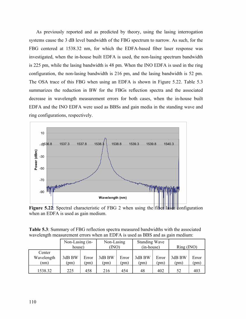
110

As previously reported and as predicted by theory, using the lasing interrogation

systems cause the 3 dB level bandwidth of the FBG spectrum to narrow. As such, for the

FBG centered at 1538.32 nm, for which the EDFA-based fiber laser response was

investigated, when the in-house built EDFA is used, the non-lasing spectrum bandwidth

is 225 pm, while the lasing bandwidth is 48 pm. When the INO EDFA is used in the ring

configuration, the non-lasing bandwidth is 216 pm, and the lasing bandwidth is 52 pm.

The OSA trace of this FBG when using an EDFA is shown in Figure 5.22. Table 5.3

summarizes the reduction in BW for the FBGs reflection spectra and the associated

decrease in wavelength measurement errors for both cases, when the in-house built

EDFA and the INO EDFA were used as BBSs and gain media in the standing wave and

ring configurations, respectively.

-90

-70

-50

-30

-10

10

1536.8 1537.3 1537.8 1538.3 1538.8 1539.3 1539.8 1540.3

Wavelength (nm)

Pow

er (d

Bm)

Figure 5.22: Spectral characteristic of FBG 2 when using the fiber laser configuration when an EDFA is used as gain medium.

Table 5.3: Summary of FBG reflection spectra measured bandwidths with the associated wavelength measurement errors when an EDFA is used as BBS and as gain medium:

Non-Lasing (in-

house) Non-Lasing

(INO) Standing Wave

(in-house) Ring (INO) Center

Wavelength (nm)

3dB BW (pm)

Error (pm)

3dB BW (pm)

Error (pm)

3dB BW (pm)

Error (pm)

3dB BW (pm)

Error (pm)

1538.32 225 458 216 454 48 402 52 403

111

5.5.3 Continuous-Time Measurement Results

The experimental results presented earlier were measured in a quasi-steady-state

manner. It is also important to investigate the dynamic response of the system, i.e., to

assess the suitability of the system to capture dynamically varying perturbations. For this

purpose, two experiments were conducted using the setup in Figure 5.23. Note that the

experiment was conducted using an RSOA (reflective SOA) as the BBS and gain

medium for the fiber laser system.

FBG 1 FBG 2 FBG 3 FBG 4Optical Coupler

SOA OutPC

Photodetector

RSOA

AWG

Oscilloscope

Figure 5.23: Experimental setup for time-domain measurements using an RSOA.

A) Strain and Temperature Effect on the Time-Domain Signal A first set of experiments were conducted using one FBG immersed in a water filled

ultrasonic bath, which emits a signal at 42 kHz. As a result, the FBG is strained or

compressed as the fiber follows the ultrasonic signal. At room temperature, when the

position of the FBG spectrum relatively to its corresponding AWG signal is as shown in

Figure 5.24, the signal measured with the oscilloscope follows a sinusoidal variation in

time, at the same frequency as the ultrasonic signal as illustrated in Figure 5.25.

112

-80

-70

-60

-50

-40

-30

-20

-10

01543.5 1543.7 1543.9 1544.1 1544.3 1544.5 1544.7 1544.9 1545.1 1545.3 1545.5

Wavelength (nm)

Pow

er (d

Bm)

Figure 5.24: The FBG and AWG spectra when the former is placed in the ultrasonic bath at 25 °C.

-30

-20

-10

0

10

20

30

0 20 40 60 80 100 120

Ampl

itude

(mV)

Time (µs)

Figure 5.25: Response to the ultrasonic signal when the FBG is placed in the ultrasonic bath at 25 °C.

On the other hand, when the temperature is increased to 50 °C, the FBG is positioned

relatively to the AWG channel as shown in Figure 5.26, and the photodetector signal as

measured with the oscilloscope experiences a higher amplitude sinusoidal variation, as

shown in Figure 5.27. As expected, when the FBG moves towards longer wavelengths

when temperature increases, the DC level follows the AWG power level. In this case, as

113

illustrated in Figure 5.28 a) and b), the DC value decreases from 3.33 V to 2.16 V

because at room temperature the spectra of the FBG and AWG overlap at a wavelength

close to the peak of the AWG spectrum, whose slope is steeper on its falling or rising

edges. As a result, at 50 °C, the ultrasonic signal is translated to an oscilloscope signal of

higher amplitude.

-80

-70

-60

-50

-40

-30

-20

-10

01543.5 1543.7 1543.9 1544.1 1544.3 1544.5 1544.7 1544.9 1545.1 1545.3 1545.5

Time (s)

Pow

er (d

Bm)

Figure 5.26: The FBG and AWG spectra when the former is placed in the ultrasonic bath and water is heated to 50 °C.

-600

-400

-200

0

200

400

600

0 20 40 60 80 100 120

Ampl

itude

(mV)

Time (µs)

Figure 5.27: Response to the ultrasonic signal when the FBG is placed in the ultrasonic bath at 50 °C.

114

0

0.5

1

1.5

2

2.5

3

3.5

4

0 0.00002 0.00004 0.00006 0.00008 0.0001 0.00012

Time (s)

Ampl

itude

(V)

a)

0

0.5

1

1.5

2

2.5

3

3.5

4

0 0.00002 0.00004 0.00006 0.00008 0.0001 0.00012

Time (s)

Am

plitu

de (V

)

b) Figure 5.28: DC amplitude level when the temperature is a) 25 °C, and b) 50 °C.

B) Strain Calibration Measurements To quantify the amount of strain applied to the FBG (center wavelength at 1538.32

nm as used in the previous experiments) by the ultrasonic signal, a calibration

measurement that maps wavelength change to mean amplitude change for the DC signal

measured using the oscilloscope is necessary. Thus, Figures 5.29 and 5.30 show the

change in wavelength and the change in DC mean amplitude, respectively as functions of

applied strain, which is quantified by placing the FBG on the strain system used to

perform the discrete measurements. These curves were then used to achieve the mapping

115

curve, whose rising or falling edges are shown in Figure 5.31 a) and b), respectively, to

achieve a one-to-one correlation between the change in wavelength with strain and the

mean amplitude measured with the oscilloscope.

y = 1.0774x + 1538.5R2 = 0.9982

1538.41538.51538.61538.71538.81538.9

15391539.11539.21539.31539.41539.5

0 0.2 0.4 0.6 0.8 1

Relative Strain (mstrain)

Wav

elen

gth

(nm

)

Figure 5.29: FBG wavelength as a function of applied strain.

02468

101214161820

0 0.2 0.4 0.6 0.8 1Relative Strain (mstrain)

Mea

n A

mpl

itude

(V)

Figure 5.30: Measured mean amplitude measured with the oscilloscope at the output of the AWG channel corresponding to the FBG under test as a function of applied strain.

116

y = 56.796x - 87386R2 = 0.979

0

2

4

6

8

10

12

14

16

18

1538.55 1538.6 1538.65 1538.7 1538.75 1538.8 1538.85 1538.9

Wavelength (nm)

Mea

n A

mpl

itude

(V)

a)

y = -42.528x + 65464R2 = 0.9889

0

2

4

6

8

10

12

14

16

1538.95 1539 1539.05 1539.1 1539.15 1539.2 1539.25 1539.3 1539.35

Wavelength (nm)

Mea

n A

mpl

itude

(V)

b) Figure 5.31: Wavelength-to-electric signal mean amplitude mapping when the FBG overlaps with a) the rising, and b) the falling edges of the AWG channel.

117

5.6 Discussion and Conclusion

The experimental results successfully demonstrate that using FBGs as part of fiber

laser systems helps improve the power efficiency of the wavelength to power mapping

procedure previously proposed, i.e., the power enhancement is about 30 dB or more.

However, when using the ring fiber laser configuration shows a gain higher by about 10

dB than the standing wave configuration. Moreover, the results also depend on the

broadband source used. As such, using an SOA as broadband source and as gain medium

shows multiple wavelengths lasing characteristic, while using an EDFA only supports

one wavelength. Experimental work using both gain media confirms the prediction that

fiber laser systems reduce the 3 dB level bandwidth. However, only a slight increase in

wavelength to power mapping resolution is observed. Moreover, using the EDFA as part

of the lasing system shows a slightly increased wavelength to power mapping resolution,

which may be accounted for by the further decrease in FBG reflection spectrum 3 dB

level bandwidth.

Note that the experiments on the FBG wavelength to power mapping systems were

performed at constant temperature. However, from a practical perspective, strain sensors

are usually used in environments that experience temperature fluctuations, which induce

wavelength changes, and may lead to erroneous wavelength to power mapping.

Therefore, to obtain reliable strain measurement, further work may involve incorporating

a temperature compensation system. Moreover, since the system relies on power

measurement, it is important that the fiber laser power levels remain stable in time and

are insensitive to external physical perturbation. For this purpose, it is important to work

with amplifiers showing relatively low polarization dependence, such that any external

disturbance to the fiber or to the FBGs does not affect the power of the lasing mode. This

is a problem encountered when using SOAs, whose gain dependence on polarization

ranges from very high to very low values. One advantage of having a gain that is highly

dependent on polarization is the ability to achieve improved wavelength selectivity;

nevertheless, small changes in fiber birefringence amount for large changes in the power

level of the lasing wavelengths. Therefore, when evaluating the performance of a fiber

laser system, it is necessary to have not only the required lasing characteristics, which for

sensor systems imposes a restraint on the number of lasing wavelengths, but also a high

118

degree of stability, which increases the chances of having reliable parameter

measurement.

119

5.7 References

[5.1] L. Zhang, W. Zhang, and I. Bennion, “In-Fiber Grating Optic Sensors” in Fiber Optic Sensors edited by Shizhuo Yin, Paul B. Ruffin, and Francis T.S. Yu, pp. 109-162, CRC Press, Boca Raton, FL, 2008.

[5.2] D.C.C. Norman, D.J. Webb, and R.D. Pechstedt, “Extended range interrogation of

wavelength division multiplexed fibre Bragg grating sensors using arrayed waveguide grating,” Electronics Letters, vol. 39, no. 24, pp. 1714 – 1716, 2003.

[5.3] F.G. Sun, G.Z. Xiao, Z.Y. Zhang, and Z.G. Lu, “Modeling of arrayed waveguide

grating for wavelength interrogation application,” Optics Communications, vol. 271, pp. 105–108, 2007.

[5.4] G.Z. Xiao, P. Zhao, F. Sun, Z. Lu, and Z. Zhang, “Arrayed-waveguide-grating-

based interrogator for wavelength-modulated multi-fiber-optic sensor applications,” IEEE Photonics Technology Letters, vol. 17, no. 8, pp.1710-1712, 2005.

[5.5] P. Niewczas, A.J. Willshire, L. Dziuda, and J.R. McDonald, “Performance

analysis of the fiber Bragg grating interrogation system based on an arrayed waveguide grating,” IEEE Transactions on Instrumentation and Measurement, vol. 53, no. 4, pp. 1992-1196, 2003.

[5.6] S. Abad, F.M. Araújo, L.A. Ferreira, J.L. Santos, and M. López-Amo,

“Interrogation of wavelength multiplexed fiber Bragg gratings using spectral filtering and amplitude-to-phase optical conversion,” Journal of Lightwave Technology, vol. 21, no. 1, pp. 127-131, 2003.

[5.7] A. Yariv and P. Yeh, “Theory of laser oscillation and some specific laser

systems” in Photonics: Optical Electronics in Modern Communications, 6th ed., pp. 237-312, Oxford University Press, New York, NY, 2007.

[5.8] C.H. Yeh, C.W. Chow, Y.F. Wu, F.Y. Shih, C.H. Wang, and S. Chi,

“Multiwavelength Erbium-doped fiber ring laser employing Fabry–Perot etalon inside cavity operating in room temperature,” Optical Fiber Technology, vol. 15, pp. 344–347, 2009.

[5.9] S. Feng, O. Xu, S. Lu, X. Mao, T. Ning, and S. Jian, “Switchable dual-wavelength

Erbium-doped fiber-ring laser based on one polarization maintaining fiber Bragg grating in a Sagnac loop interferometer,” Optics and Laser Technology, vol. 41, pp. 264– 267, 2009.

[5.10] X. Liu, “A novel dual-wavelength DFB fiber laser based on symmetrical FBG

structure,” IEEE Photonics Technology Letters, vol. 19, no. 9, pp. 632-634, 2007.

120

[5.11] Y. Liu, X. Dong, P. Shum, S. Yuan, G. Kai, and X. Dong, “Stable room-temperature multi-wavelength lasing realization in ordinary Erbium-doped fiber loop lasers,” Optics Express, vol. 14, no. 20, pp. 9293-9298, 2006.

[5.12] O. Xu, S. Lu, S. Feng, Z. Tan, T. Ning, and S. Jian, “Single-longitudinal-mode

Erbium-doped fiber laser with the fiber-Bragg-grating-based asymmetric two-cavity structure,” Optics Communications, vol. 282, pp. 962–965, 2009.

[5.13] W. Guan and J.R. Marciante, “Dual-frequency operation in a short-cavity

Ytterbium-doped fiber laser,” IEEE Photonics Technology Letters, vol. 19, no. 5, pp. 261-263, 2007.

[5.14] Z. Zhang, J. Wu, K. Xu, X. Hong, and J. Lin, “Tunable multiwavelength SOA

fiber laser with ultra-narrow wavelength spacing based on nonlinear polarization rotation,” Optics Express, vol. 17, no. 19, pp. 17200-17205, 2009.

[5.15] D.S. Moon, B.H. Kim, A. Lin, G. Sun, W.-T. Han, Y.-G. Han, and Y. Chung,

“Tunable multi-wavelength SOA fiber laser based on a Sagnac loop mirror using an elliptical core side-hole fiber,” Optics Express, vol. 15, no. 13, pp. 8371-8376, 2007.

[5.16] H. Ahmad, A. H. Sulaiman, S. Shahi, and S.W. Harun, “SOA-based multi-

wavelength laser using fiber Bragg gratings,” Laser Physics, vol. 19, no. 5, pp. 1002–1005, 2009.

[5.17] S. Tanaka, K. Inamoto, H. Yokosuka, H. Somatomo, and N. Takahashi, “Multi-

wavelength tunable fiber laser using SOA: application to fiber Bragg grating vibration sensor array,” IEEE Sensors Conference, pp. 411-414, 2007.

[5.18] N.Y. Voo, P. Horak, M. Ibsen, and W.H. Loh, “Linewidth and phase noise

characteristics of DFB fibre lasers” in SPIE European Symposium on Optics and Photonics in Security and Defence, vol. 5620, pp. 179-186, London, 2004.

[5.19] H. Su and X.G. Huang, “A novel fiber Bragg grating interrogating sensor system

based on AWG demultiplexing,” Optics Communications, vol. 275, pp. 196–200, 2007.

[5.20] G.Z. Xiao, P. Zhao, F.G. Sun, Z.G. Lu, Z. Zhang, and C.P. Grover, “Interrogating

fiber Bragg grating sensors by thermally scanning a demultiplexer based on arrayed waveguide gratings,” Optics Letters, vol. 29, no. 19, pp. 2222-2224, 2004.

[5.21] X.J.M. Leijtens, B. Kuhlow, and M.K. Smit, “Arrayed Waveguide Gratings” in

Wave-length Filters in Fibre Optics by H. Venghaus, pp. 125-187. Springer-Verlag Berlin Heidelberg: Berlin, Germany, 2006.

121

[5.22] O. Frazão, S.F.O. Silva, A. Guerreiro, J.L. Santos, L.A. Ferreira, and F.M. Araújo, “Strain sensitivity control of fiber Bragg grating structures with fused tapers,” Applied Optics, vol. 46, no. 36, pp. 8578-8582, 2007.

[5.23] Y. Zhao and Y. Liao, “Discrimination methods and demodulation techniques for

fiber Bragg grating sensors”, Optics and Lasers in Engineering, vol. 41, pp. 1-18, 2004.

122

6. Conclusion and Future Work

This thesis proposes and demonstrates the feasibility of using a number of

interrogation systems for FBG-based sensors. As presented in Chapter 2, understanding

the theory behind such sensors, and acquiring knowledge about previous work performed

toward designing practical detection systems are important for identifying existing issues.

This leads to finding cost effective and reliable solutions. Moreover, before

commercialization, it is important to make sure the sensors can be reliably used.

Therefore, Chapter 3 provided an example of characterizing a ready-to-be-

commercialized vibration sensor based on a twin FBG pair, and the tests performed on

them include operability region, sensor reliability, which is given by the ability of the

sensor to measure a unique value for every vibration amplitude and frequency conditions.

It was found that a typical calibration curve is linear, with the slope giving the sensor’s

sensitivity. Moreover, it is important to make sure that, for a given vibration condition,

the measurement does not vary considerably, so the system does not measure a different

condition than the real one, thus leading to detection errors. In the same chapter, it was

found that multiplexing requires a trade-off between the sensor design and the sensing

requirements, i.e., if the sensors are designed to acquire data over long distances, the

maximum number of sensors can be tailored by increasing the reflectivity of the last

sensor in the array, or by decreasing the reflectivities of the preceding FBGs. Another

alternative would be to increase the power sent to the multiplexed sensors. On the other

hand, for pre-defined system conditions, the number of sensors that can be time-division

multiplexed can be increased by decreasing the length span over which sensing is

performed.

Chapter 4 presents an extension of the basic design of the vibration sensor to achieve

either temperature or strain measurements. As discussed, temperature measurement is

used to prove that the ability of the FBG pair structure to slice a broadband beam can be

used to tune the peak of a single passband MPF. It was found that, for given temperature

conditions, the MPF has a unique value that depends on the dispersion characteristic of

the fiber in response to the change experienced by the FBG pair reflection spectrum: both

the center wavelength and the FSR of the interference signal increase with temperature;

123

however, the former changes more compared to the latter. It was demonstrated that,

driving the modulator in the MPF system with an RF signal falling on either the rising or

the falling edge of the pass-band of the filter results in a linear change in the measured

power at the output. It was observed that the MPF characteristic changes so different

linearity and sensitivities are obtained—this gives flexibility to the measurement system.

For the proposed system, the delay component was an 85 km long SMF, which added

loss to the system and made it unpractical. Therefore, future work involves designing the

FBG pair so the interference pattern FSR increases, e.g. decrease the separation between

the FBGs. Moreover, keeping the sensor design intact, a shorter length of higher

dispersion fiber can be used as the MPF delay element to obtain the observed filtering

characteristics. In terms of application, in the future the sensor may be used as

temperature compensation component when measuring vibration or strain. Note that the

latter can greatly benefit from using an MPF system, which is characterized by high

speed capability and would allow the fast real-time monitoring of strain.

A second system presented in Chapter 5 provided a solution to obtaining portable,

cost effective, and power efficient interrogation systems for FBG strain or temperature

sensors. The experimental work treated the measurement of strain, and it involved using

an AWG to map the wavelength-encoded information to a power measurement, which

allows using cheap and portable instrumentation such as power meters to detect the

changes in the FBG reflection spectrum with strain. Moreover, the system was designed

in a fiber laser configuration, which provided amplified power (by up to 35 dB), thus

increasing the power efficiency of the system. Another aspect that was investigated in

this work is the effect the gain medium has both the lasing characteristic of the system

(power efficiency) and on the mapping characteristics. The two BBS explored were

SOAs and EDFAs. It was found that the former experiences better lasing behaviour than

the latter, which, even though it provides slightly improved mapping, experiences single

wavelength lasing, and this prevents the effective use of WDM sensor systems. For this

work, future work involves investigating the number of sensors supported by the lasing

system, i.e., for a given BBS and gain medium, what would the maximum number of

sensors that experience lasing with equalized power levels be. Moreover, in general lasers

experience instabilities with changing polarization or fiber birefringence, and, therefore,

124

for practical applications, it is important to characterize the system in terms of stability.

Another important parameter that needs to be explored to extend the study to practical

applications would be achieving a practical temperature compensation scheme.

Interrogation Systems for Fiber Bragg Grating-Based...

Documents

Transcript of Interrogation Systems for Fiber Bragg Grating-Based...