Interpreting Opinion Polls Example1: (Confidence Interval for the population proportion): Suppose...
86
Interpreting Opinion Polls Example1: (Confidence Interval for the population proportion) : Suppose that the result of sampling yields the following: p= 0.4 ; n = 36. Use this information to construct a 98% CI for . Recall from, last week 98% CI for is [0.21 0.59]
-
date post
20-Dec-2015 -
Category
Documents
-
view
218 -
download
0
Transcript of Interpreting Opinion Polls Example1: (Confidence Interval for the population proportion): Suppose...

Interpreting Opinion Polls
Example1: (Confidence Interval for the population proportion): Suppose that
the result of sampling yields the following:
p= 0.4 ; n = 36. Use this information to construct a
98% CI for .
Recall from, last week
98% CI for is [0.21 0.59]

Interpreting Opinion Polls
Labour 45 pointsConservatives 39 pointsLib. Dems 15 pointsOther 1 point
Margin of Error :Typically, this means that population proportion of labour voters is between 42% and 48% (with 95% confidence)

Hypothesis Testing

x
Two competing Hypotheses
The Null Hypothesis (H0):The population mean ( =20The Alternative Hypothesis (H1):The population mean ( =25

x
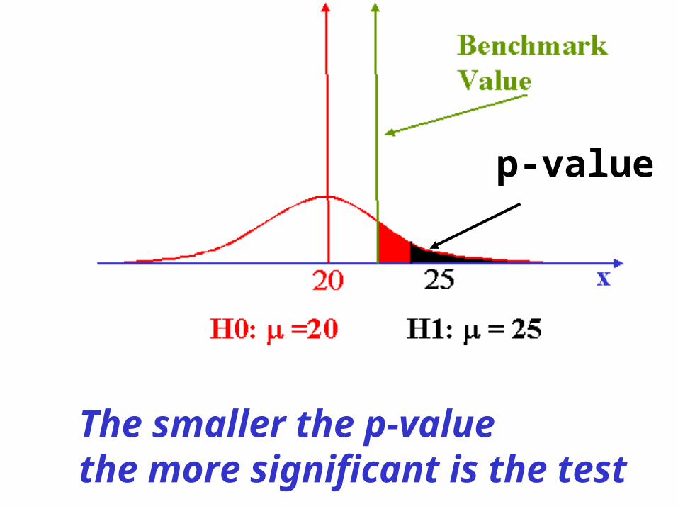
H0: =20 H1: = 25

x
H0: =20 H1: = 25
BenchmarkValue
p-value

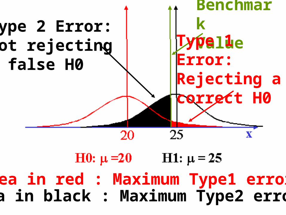
BenchmarkValueType 2 Error:
Not rejectingA false H0
Type 1 Error:Rejecting a correct H0
Area in black : Maximum Type2 errorArea in red : Maximum Type1 error

BenchmarkValue
MaximumType 1 ErrorMaximum
Type 2 Error:

BenchmarkValue
MaximumType 1 ErrorMaximum
Type 2 Error

The Spirit of Hypothesis Testing
H0 is the hypothesis that is challenged
H0 is the established hypothesis

Xo
y
Can we have intersecting indifference curves?
a
a ~ b, a ~ c; so b ~ca contradiction of the axiom more is better
bc
H0 : Yes H1 : No
We work under the assumption that H0 is correct!

x
H0: = 0 H1: = 1

SignificanceLevel (
The Maximum Type 1 Error= SignificanceLevel

The smaller the p-value the more significant is the test
p-value

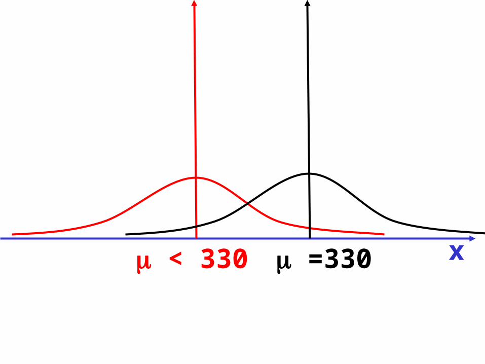
Fizzy drink cans should have 330 ml of content on average. A consumer group has complained against a manufacturer that its contents are lessthen the stated amount. Use the following data to assess the complaint.(Assume a normal population)
One-Tail and Two-Tail Tests

x < 330 =330

xMEAN = 320 ; = 10 ; n = 16
Step 1: Set up the hypotheses
H0 :
H1 :
Step 2: Select statistic
One-Tail Test

The statistic to be used is xMEAN = 320
Step3 : Identify the distributionof xMEAN
xMEAN ~ Normal16
xMEAN ~ Normal16 Under H0

Step 4: Construct test statistic (z) z= {(xMEAN –} = (320-330)/10/4 = -4
Step 5: Compare with critical value zC
zC = -1.645 > -4
zC = -1.645 for a one-tailed test with significance level () = 0.05

Step 6 : Draw conclusion
The test is significant. Reject H0 at 5% and at 1% ( -4 < -2.33)
Step 7: Interpret result
zC = -1.645 for a one-tailed test with significance level () = 0.05
There is overwhelming evidence to support the claim !

A cereal manufacturer is concerned that the boxes of cereal not be under-filled orover-filled. Each box is supposed to contain 130 grams of cereal. A test is done to see whether the machines are putting an average of 130 grams into a single box. A random sample of 30 boxesis tested. The average weight is found out to be 128 grams and the sample standard deviation 10 grams.
A Two-Tail Test

x < 130 =130 >130

Set up the hypotheses to test whether the average number of grams per box isdifferent from 130. Step 1 H0 :
H1 :
Two-Tail Test
Perform the test at 10% level of significance.

Step3 : Identify the distributionof xMEAN
xMEAN ~ 30
xMEAN ~ Normal30 (approx.)
Under H0
Step 2: Select statisticThe statistic to be used is xMEAN = 128

Step 4: Construct test statistic (z) z= {(xMEAN –} = (128-130)/10/ = -1.1
Step 5: Compare with critical value zC
zC = 1.645 for a two-tailed test with significance level () = 0.1
1.645 < 1.1

Explain which hypothesis you are rejecting and why. Do you think the decision to accept/reject the null hypothesis stays unchanged if the significance level is lowered to 5%? Explain carefully.

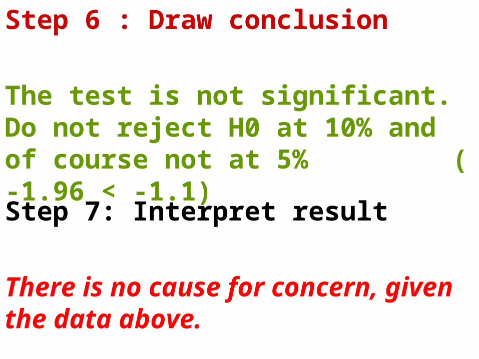
Step 6 : Draw conclusion
The test is not significant. Do not reject H0 at 10% and of course not at 5% ( -1.96 < -1.1)
Step 7: Interpret result
There is no cause for concern, given the data above.

A production process makes components whose strengths are normally distributedwith mean 40kg and unknown variance.
The process is modified and 12 components are selected at random withMean strength 41.125kg and sample standard deviation 1.316591 kg.
Is there any evidence that the modifiedProcess makes stronger components?

Step 1 : Set up the hypothesesH0 : H1 :
One-Tail Test
Perform the test at 5% level of significance.
Step 2: Select statistic
The statistic to be used is xMEAN = 41.125

Step3 : Identify the distribution
(xMEAN – /s/n has a t-distribution of 11 degrees of freedom
Step 4: Construct test statistic (t) {(xMEAN –}/s/} = (41.125-40)/ 1.316591 /

Step 5: Compare with critical value tC
tC = 1.795884 for a one-tailed test with significance level () = 0.05 and d.o.f . =11t = 2.96 > 1.795884Step 6 : Draw conclusion The test is significant. Reject H0 at 5% ( 2.96 > 1.795884) and at 1% (2.96 > 2.718) 0.006488 is the prob of type 1 error

Step 7: Interpret results
There is overwhelming evidence that the modified process makes stronger components
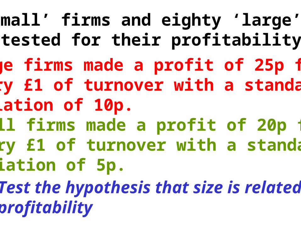
100 ‘small’ firms and eighty ‘large’ firms were tested for their profitability.
Large firms made a profit of 25p for every £1 of turnover with a standard deviation of 10p.Small firms made a profit of 20p for every £1 of turnover with a standard deviation of 5p.Test the hypothesis that size is related toprofitability

x = large firm; y = small firm
xMEAN = 25; sX = 10 nX =80yMEAN = 20; sy = 5 ; nY =100
Step 1 H0 : x
- Y = 0H1 : x
- Y Two-Tail Test
Perform the test at 5% level of significance.

Step3 : Identify the distributionof xMEAN -yMEAN
xMEAN -yMEAN ~ Normalx
YX 80 + Y 100
~ NormalsX 80 + sY 100(approx.) Under H0
Step 2: Select statisticThe statistic to be used is xMEAN -yMEAN = 25-20 = 5
~ Normal10080 + 25100(approx.)

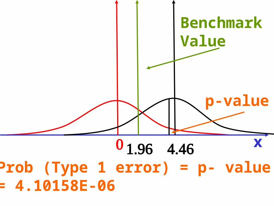
Step 4: Construct test statistic (z) z= {(xMEAN -yMEAN –(x
–Y} = (5-0)/ = 4.46
Step 5: Compare with critical value zC
zC = 1.96 for a two-tailed test with significance level () = 0.05
1.96 < 4.46

Step 6 : Draw conclusion
The test is significant. Reject H0 at 5% ( 1.96 < 4.46) or even at 1%
Step 7: Interpret result
There is overwhelming evidence that large firms are more profitable
x
BenchmarkValue
p-value
Prob (Type 1 error) = p- value = 4.10158E-06
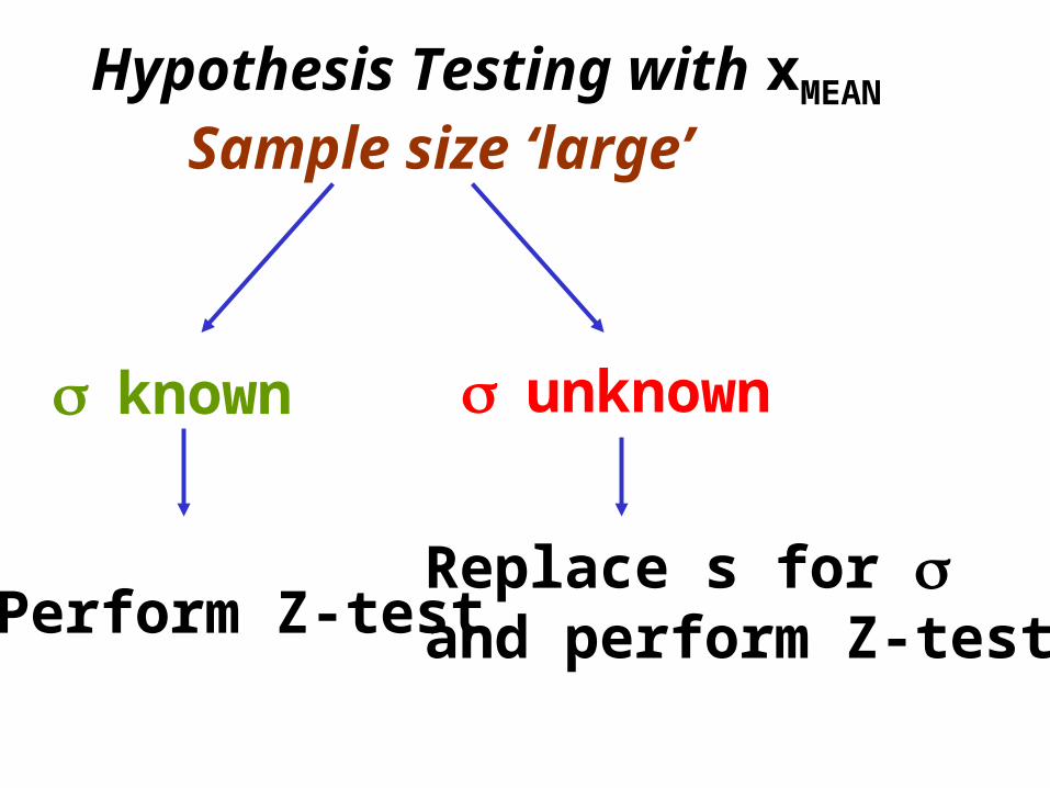
Sample size ‘large’Hypothesis Testing with xMEAN
known unknown
Perform Z-testReplace s for and perform Z-test

Sample size ‘small’
Normal Population
known unknown
Non-normal Population
Parametric TestNot possiblePerform Z-test Perform t-test.
Replace s for

Learning ObjectivesLearning Objectives
• Understand the logic of hypothesis testing, and know how to establish null and alternate hypotheses.
• Understand Type I and Type II errors.• Use large samples to test hypotheses about a
single population mean and about the differences of two population means
• Use large samples to test hypotheses about a single population proportion and about the differences of two population proportions

• Test hypotheses about a single population mean using small samples when is unknown and the population is normally distributed.

Hypothesis Testing
A process of testing hypotheses about parameters by setting up null and alternative hypotheses, gathering sample data, computing statistics from the samples, and using statistical techniques to reach conclusions about the hypotheses.
Null and Alternative HypothesesNull and Alternative Hypotheses
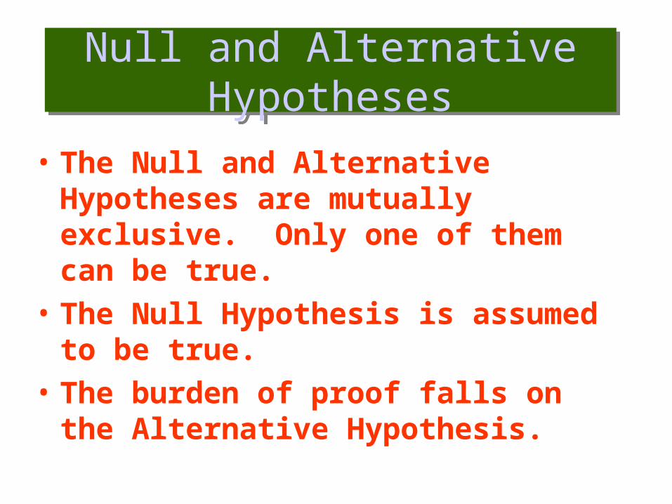
• The Null and Alternative Hypotheses are mutually exclusive. Only one of them can be true.
• The Null Hypothesis is assumed to be true.
• The burden of proof falls on the Alternative Hypothesis.

The Spirit of Hypothesis Testing
H0 is the hypothesis that is challenged
H0 is the established hypothesis

Xo
y
Can we have intersecting indifference curves?
a
a ~ b, a ~ c; so b ~ca contradiction of the axiom more is better
bc
H0 : Yes H1 : No
We work under the assumption that H0 is correct!

Null and Alternative Hypotheses: ExampleNull and Alternative
Hypotheses: Example
• A soft drink company is filling 12 oz. cans with cola.• The company hopes that the cans are averaging 12
ounces.
H oz
H oz
o
a
:
:
12
12
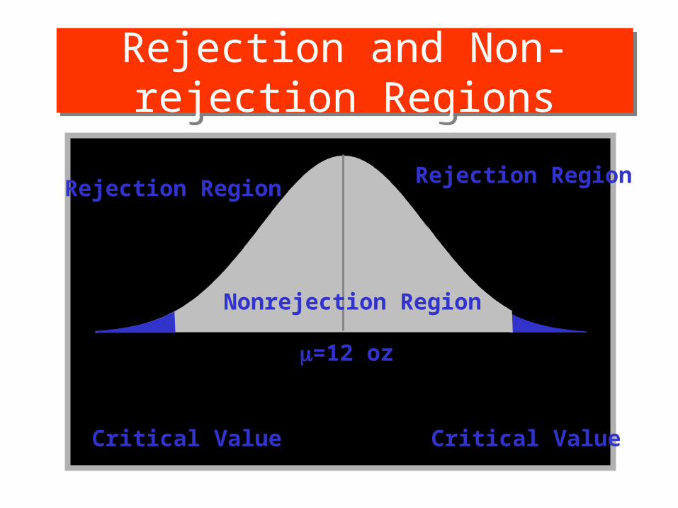
Rejection and Non-rejection Regions
Rejection and Non-rejection Regions
=12 oz
Nonrejection Region
Rejection Region
Critical Value
Rejection Region
Critical Value

Type I and Type II ErrorsType I and Type II Errors
• Type I Error– Rejecting a true null hypothesis – The probability of committing a Type I error
is called , the level of significance.• Type II Error
– Failing to reject a false null hypothesis– The probability of committing a Type II
error is called .– Power is the probability of rejecting a false
null hypothesis, and equal to 1-

x
H0: =20 H1: = 25
Two competing Hypotheses

x
H0: =20 H1: = 25
BenchmarkValue
p-value
BenchmarkValueType 2 Error:
Not rejectingA false H0
Type 1 Error:Rejecting a correct H0
Area in black : Maximum Type2 errorArea in red : Maximum Type1 error

BenchmarkValue
MaximumType 1 ErrorMaximum
Type 2 Error:

The smaller the p-value the more significant is the test
p-value
SignificanceLevel (
The Maximum Type 1 Error= SignificanceLevel

Decision Table for Hypothesis Testing
Decision Table for Hypothesis Testing
(
( )
Null True Null False
Fail toreject null
CorrectDecision
Type II error
Reject null Type I error
Correct Decision (Power)
The smaller the p-value the more significant is the test
p-value

Fizzy drink cans should have 330 ml of content on average. A consumer group has complained against a manufacturer that its contents are lessthen the stated amount. Use the following data to assess the complaint.(Assume a normal population)
A One-Tail Test
x < 330 =330

xMEAN = 320 ; = 10 ; n = 16
Step 1: Set up the hypotheses
H0 :
H1 :
Step 2: Select statistic
One-Tail Test

The statistic to be used is xMEAN = 320
Step3 : Identify the distributionof xMEAN
xMEAN ~ Normal16
xMEAN ~ Normal16 Under H0

Step 4: Construct test statistic (z) z= {(xMEAN –} = (320-330)/10/4 = -4
Step 5: Compare with critical value zC
zC = -1.645 > -4
zC = -1.645 for a one-tailed test with significance level () = 0.05

Step 6 : Draw conclusion
The test is significant. Reject H0 at 5% and at 1% ( -4 < -2.33)
Step 7: Interpret result
zC = -1.645 for a one-tailed test with significance level () = 0.05
There is overwhelming evidence to support the claim !

A cereal manufacturer is concerned that the boxes of cereal not be under-filled orover-filled. Each box is supposed to contain 130 grams of cereal. A test is done to see whether the machines are putting an average of 130 grams into a single box. A random sample of 30 boxesis tested. The average weight is found out to be 128 grams and the sample standard deviation 10 grams.
A Two-Tail Test

x < 130 =130 >130

Set up the hypotheses to test whether the average number of grams per box isdifferent from 130. Step 1 H0 :
H1 :
Two-Tail Test
Perform the test at 10% level of significance.

Step3 : Identify the distributionof xMEAN
xMEAN ~ 30
xMEAN ~ Normal30 (approx.)
Under H0
Step 2: Select statisticThe statistic to be used is xMEAN = 128

Step 4: Construct test statistic (z) z= {(xMEAN –} = (128-130)/10/ = -1.1
Step 5: Compare with critical value zC
zC = 1.645 for a two-tailed test with significance level () = 0.1
1.645 < 1.1
Step 6 : Draw conclusion
The test is not significant. Do not reject H0 at 10% and of course not at 5% ( -1.96 < -1.1)
Step 7: Interpret result
There is no cause for concern, given the data above.

100 ‘small’ firms and eighty ‘large’ firms were tested for their profitability.
Large firms made a profit of 25p for every £1 of turnover with a standard deviation of 10p.Small firms made a profit of 20p for every £1 of turnover with a standard deviation of 5p.Test the hypothesis that size is related toprofitability

x = large firm; y = small firm
xMEAN = 25; sX = 10 nX =80yMEAN = 20; sy = 5 ; nY =100
Step 1 H0 : x
- Y = 0H1 : x
- Y Two-Tail Test
Perform the test at 5% level of significance.

Step3 : Identify the distributionof xMEAN -yMEAN
xMEAN -yMEAN ~ Normalx
YX 80 + Y 100
~ NormalsX 80 + sY 100(approx.) Under H0
Step 2: Select statisticThe statistic to be used is xMEAN -yMEAN = 25-20 = 5
~ Normal10080 + 25100(approx.)

Step 4: Construct test statistic (z) z= {(xMEAN -yMEAN –(x
–Y} = (5-0)/ = 4.46
Step 5: Compare with critical value zC
zC = 1.96 for a two-tailed test with significance level () = 0.05
1.96 < 4.46

Step 6 : Draw conclusion
The test is significant. Reject H0 at 5% ( 1.96 < 4.46) or even at 1%
Step 7: Interpret result
There is overwhelming evidence that large firms are more profitable

Example: Thirty-five percent of the consumers were dissatisfied with the Product when a new CEO was elected.
Test of Proportion
Five months later, 108 out of 360 were found out to be dissatisfied.
Can we conclude (at 5%) that the newly elected CEO has significantly reduced the level of dissatisfaction amongst consumers?
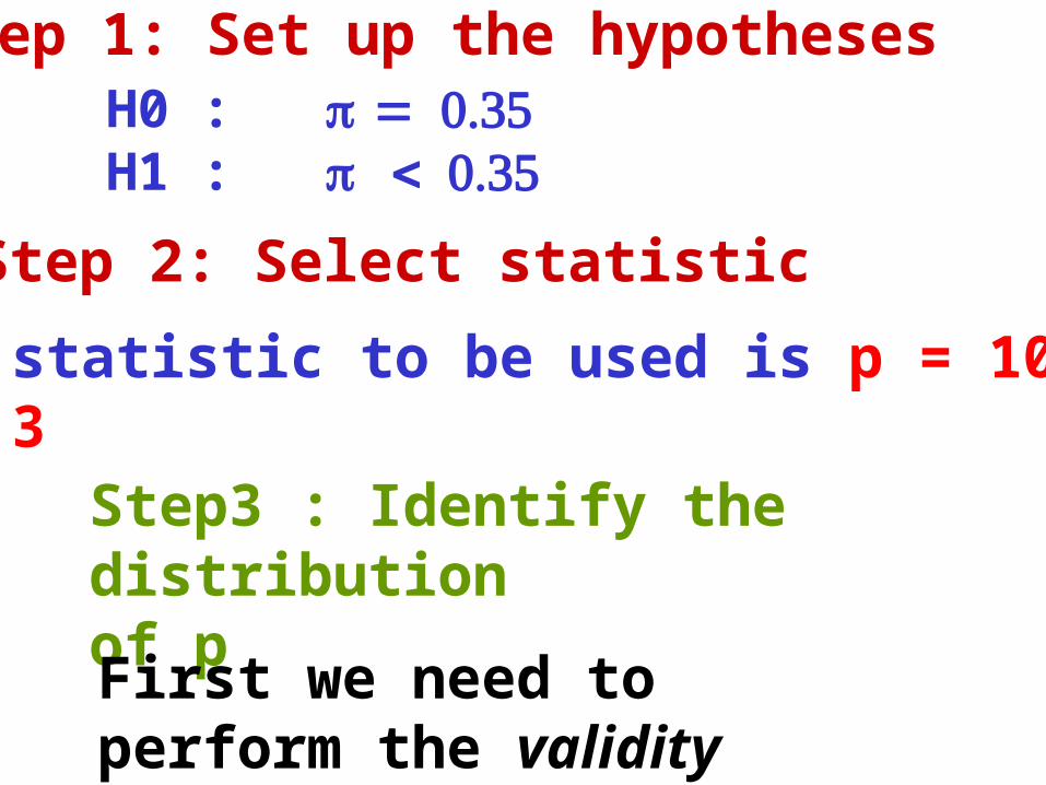
Step 2: Select statistic
The statistic to be used is p = 108/360 = 0.3Step3 : Identify the distributionof p
First we need to perform the validity check
H0 : H1 :
Step 1: Set up the hypotheses

Here n = 360 and = 0.35 under H0. So the validity check is satisfied.
This means that p ~ Normal(360 where 2 = X 0.65 = 0.2275Step 4: Construct test statistic (z) z= {(p –0.350.2275)/360} = (0.3-0.35)/0.477/18.97367 -19.9

Step 5: Compare with critical value zC
zC = -19.9 < -1.645 Step 6 : Draw conclusion
The test is significant. Reject H0
Step 7: Interpret result
Based on the analysis of data, we conclude that there is strong evidence that consumer dissatisfaction has been significantly reduced.
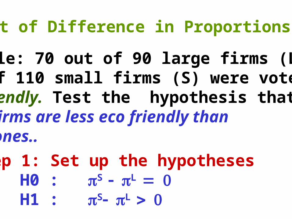
Example: 70 out of 90 large firms (L) and100 of 110 small firms (S) were voted eco-friendly. Test the hypothesis that large firms are less eco friendly than small ones..
Step 1: Set up the hypothesesH0 : S L H1 : SL
Test of Difference in Proportions

Step 2: Select statistic
The statistic to be used is pS–pL
where pL = 7/9 = 0.78; pS = 10/11 = 0.9
Step3 : Identify the distributionof pS –pL

First we need to perform the validity check
Here nS = 110 and nL = 90 but S and L
are unknown. So we perform the validity check by using the values of pS and pL for S and L respectively. The validity check is satisfied.This means that (pS - pL) ~ Normal(S L S
nS LnL

Under H0, (L S) = 0
Also, S = S S)
and L = L L )
Usep = (nS pS + nL pL) / (nS + nL ) for both S and L . Thusp = [(100/110) *110 + (70/90)*90]/200 = 0.85

Hence, S ) = 0.1275
Similarly, L ) = 0.1275
(pS - pL) ~ Normal( 0.1275110 0.127590 (pS - pL) ~ Normal(
Step 4: Construct test statistic (z) z= {(pS - pL) –0}/(0.059) = (0.9-0.78)/0.059 2

Step 5: Compare with critical value zC
zC = 1.645 < 2 Step 6 : Draw conclusion
The test is significant. Reject H0 at 5% but not at 1% ( 2 < 2.33)
Step 7: Interpret result
Based on the analysis of data, we conclude that there is enough evidence that small forms are significantly more eco-friendly.

Two-tailed Test: Small Sample, Unknown, = .05 (Part 1)
Two-tailed Test: Small Sample, Unknown, = .05 (Part 1)
Weights in Pounds of a Sample of 20 Plates
22.622.2 23.2 27.4 24.527.026.6 28.1 26.9 24.926.225.3 23.1 24.2 26.125.830.4 28.6 23.5 23.6
X 2551. , S = 2.1933, and n = 20

Two-tailed Test: Small Sample, Unknown, = .05 (Part 2)
Two-tailed Test: Small Sample, Unknown, = .05 (Part 2)
Critical Values
Rejection Regions
ct 2 093. ct 2 093.
2
025.2
025.
H
H
o
a
:
:
25
25
df n 1 19

Two-tailed Test: Small Sample, Unknown, = .05 (Part 3)
Two-tailed Test: Small Sample, Unknown, = .05 (Part 3)
tXS
n
2551 25 0
2 1933
20
104. .
. .
Since t do not reject H .o 104 2 093. . ,Critical Values
Non Rejection Region
Rejection Regions
ct 2 093. ct 2 093.
2
025.2
025.
If t reject H .
If t do not reject H .
o
o
2 093
2 093
. ,
. ,