Interpreting Aircraft Observations of Greenhouse Gases

GHG Summer School 2016 – Southampton

Grant Allen (grant.allen@manchester.ac.uk)

This class: Intro & Learning outcomes

• What can (and can’t) aircraft data do for GHG science?

• An introduction to the FAAM aircraft and its measurement suite

• Case study examples of FAAM use for measurement-led investigations

• How to analyse and interpret aircraft data

• IDL computer exercise:

- An intro to real FAAM data

- Interpretation methods and tools

Aircraft vs other sampling platforms

Method Pros Cons

Ground-based in situ Precision measurement Dense sampling/representivity of the immediate environment

Only represents a point in space and time (relies on air coming to the instrument)

Aircraft in situ Wide coverage (100s km) Precision measurement Mapping Planned sampling

Inability to sample whole areas simultaneously Difficult to plan in a “dynamic” environment

Ground remote sensing Wide spatial coverage (~km) Less precise Needs knowledge of dynamics

Satellite remote sensing (aka Earth Observation)

Global Coverage and mapping Continuous datasets

Long (poor) repeatability Poor precision Poor spatial resolution (100s m – 10km)

Regional Models Able to model processes at scales of human interaction

Unable to scale up to global, long-term impacts

Global Models Able to extrapolate to the far future

Lacks detailed process and scale interactions

What science can aircraft facilitate?

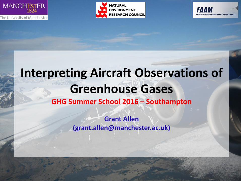
Uses the atmosphere as a natural laboratory for:

• Atmospheric chemistry and air quality

• Source apportionment and fluxes (inc. GHGs)

• Airmass characterisation and transport

• Cloud microphysics

• Radiative transfer processes and energy budgets

• Numerical Weather Prediction

• Land-air-sea interactions

• Coupled processes (e.g. aerosol-cloud interactions)

• Spatial scalability and scale-coupled processes (e.g. gravity waves, cloud evolution, plume chemistry)

What science can aircraft facilitate?

• Aircraft are a very useful bridging tool that link datasets at various scales as well as providing tailored datasets that are useful in isolation.

• Careful flight planning is required to make the most of the sampling. This requires:

- A prior hypothesis to be tested - A flight design that tests the hypothesis, constrained by

practicalities such as weather on the day, flight area restrictions etc - Flexibility for decision-making in the air based on realtime

observations

• Careful post-flight analysis is needed to make sense of the data. Aircraft data analysis is unique in that it is multi-dimensional and not uniformly gridded in space and time. As such, it often demands a forensic approach, where the data are the clues that lead the investigation – there is no set formula for aircraft data analysis and every flight is different.

Quantifying Emissions: The problem of scales

1 m 10 m 100 m 1 km 10 km 100 km

Urban modelling

THE MISSING LINK Satellites Fixed remote sensing

Emission sources Regional models Global models

In situ sampling

•The Problem: Processes/modelling/understanding at small (e.g. urban) scales

not easily extrapolated to large (global) scales

•A solution: Airborne in situ and aircraft remote sensing at local-to-regional

scales: to test models with measurements that link these scales, e.g. Karion et

al., Mays et al.

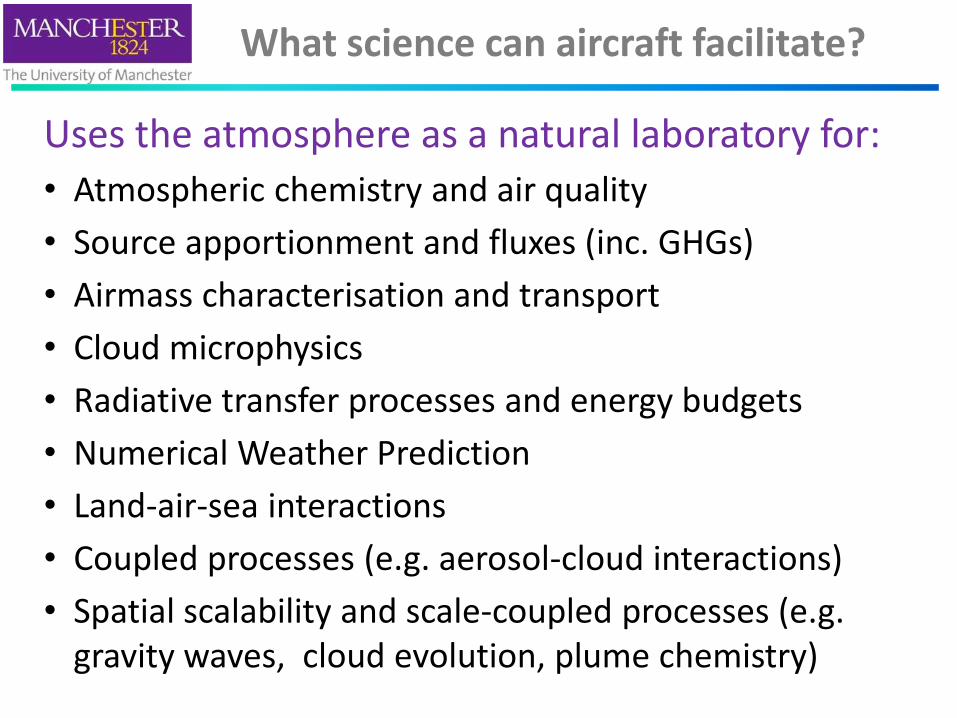
The FAAM Aircraft

FAAM Measurement suite

• In situ (1-32 Hz) • CH4, CO2 , N2O

(Aerodyne QCL, LGR FGGA)

• CO, O3, NOx,

• Dropsondes (T, p, q, winds)

• GPS, aircraft configuration

• Chemical Ionization MS (HNO3, HCN, HCOOH)

• Aerosol size, number, chemical functionality

• Whole Air Sample (WAS) system – 64 x 3 litre silico-steel canisters

– GCxGC: C6-C13 NMHC, oxygenated VOCs

– Continuous flow GC - Trace gases and CH4 d13C

• Remote sensing • Nadir open-path FTIR (ARIES)

• Vertical profiles of CH4, N2O, O3 etc

• Cloud/Aerosol lidar

Aircraft analysis: An example from VOCALS

8000

6000

4000

2000

0

Alt

itu

de

(k

m)

-80 -78 -76 -74 -72 -70 -68

Longitude

80

70

60

50

40

CO

(pp

b)

FAAM flight B412

Two meteorological periods:

•Period 1: 15th-31st Oct Surface anti-cyclone, unstable STJ, Variable FT airmass history

•Period 2: 3rd-12th Nov UT anti-cyclone, steady STJ, consistent FT history.

• Frequent pollution layers in the FT were observed (especially near the coast) in Period 1 (below)

Period 1 – Free troposphere

•FT has a gradient in source origin Continental PBL sources near the coast

•Descended long-range remote sources west of 75 W.

•Uplift to UT may have frozen in some pollution signatures and removed others

Period 2

Much more consistent marine MBL origins for all FT air along 20 S

All but the trajectories very near to shore have a remote origin.

U

dx

dy

Single wind vector

Temperature inversion, z1

CH4 well-mixed vertically

Boundary layer mass balance

U

dx

dy

Single wind vector

Temperature inversion, z1

CH4 well-mixed vertically

Surface flux = outflow – inflow

U

dx

dy

Single wind vector

Temperature inversion, z1

CH4 well-mixed vertically

Surface flux = outflow – inflow

1

0

4 ..

Z

ndzdx

dCHUflux

Mass Balancing Flux Strategy

Flux = (SijA

B

ò0

z

ò - S0 ).nij.U^ij.dx.dz

London Case study during Olympics 2012

Complimentary to the ClearfLo

Westerly winds from the Atlantic and Arctic

Flight B724 - 30 July 2012

Flight B724 - 30 July 2012

. 53.5

53.0

52.5

52.0

51.5

51.0

50.5

La

titu

de

210-1-2

Longitude

Greater London FAAM BAe 146 Wind direction Vertical plane Data used for kriging BT Tower

A

B

58

56

54

52

50

La

titu

de

-10 -8 -6 -4 -2 0 2

Longitude

b)

a)

Flight B724 – 30 July 2012 - Olympics

Urban enhancement of CH4 and CO ~50 ppb near the surface

NAME dispersion modelling

• Influence of London emissions on air sampled by the aircraft along plane AB

• Determined using backwards NAME runs for 10000 particles released from

the GPS of the aircraft.

• Warm colours show regions of greater airmass influence from London and

vice versa for darker colours.

Fluxes through downwind plane

CO2 CO CH4

Background (ppb)

385.8 ± 1.4 ppm 96 ± 5 1883 ± 8

Peak enhancement (ppb)

13.3 ppm (3%) 30 (31%) 73 (4%)

Flux AB (mol s-1) 38453 ± 3346 253 ± 11 264 ± 16

Flux AB London (mol s-1)

35861 ± 2553 219 ± 8 238 ± 12

NAEI flight track (mol s-1)

67904 462 n/a

NAEI Greater London (mol s-1)

15294 98 71

• Downwind CO2 flux in between London NAEI and regional NAEI aggregate flux

• CO flux lower than both London and regional NAEI

• CH4 flux 3 times higher than London inventory alone

Fluxes through downwind plane

Location Year Season

Flux (μmol m-2 s-1)

CO2 CO CH4

This study (mass balance) London 2012 Summer 21 ± 3 0.12 ± 0.02 0.13 ± 0.02

This study (eddy-cov.) a London 2012 Summer 1 to 83

(28 ± 17)

0.01 to 0.37

(0.15 ± 0.08)

Font et al. (2013)b London 2011 Autumn 46 to 104

Helfter et al. (2011)c London 2007 Year round 7 to 47

Harrison et al., (2012)d London 2007/08 Autumn 0.25 / 0.17

Rigby et al. (2008)e London 2006 Year round 18 ± 28

Mays et al. (2009)h Indianapolis 2008 Spring 19.2 ± 15.4 0.14 ± 0.1

a Range of the fluxes at the BT tower averaged for Summer 2012 (numbers in brackets show fluxes for 30 September 2012). b mass balance flux range using airborne measurements from 4 flights c EC range d EC means for 2 autumn periods e boundary layer model, average emission rate for winter period. h mass balance flux range from 8 flights i EC range of fluxes. k EC mean daytime flux.

MAMM, Methane in the Arctic: Measurement and Modelling

(Pyle et al., poster B33K-0613) (www.arctic.ac.uk)

Arctic Airborne Measurement

July 2012 6 flights

August 2013 9 flights

September 2013 7 flights

Photo: John Pyle

Wetland CH4 flux Survey

22 July 2012

Wetland Survey

22 July 2012

U

Transects parallel to the wind vector

22 July 2012 West East

Photo: John Pyle

Flux (mg hr-1 m-2)

CH4 CO2

Eastward transect 1.1 ± 0.6 -375 ± 202

Westward transect 1.6 ± 0.5 -357 ± 135

Both transects 1.2 ± 0.5 -350 ± 143

Whole air samples 1.0 ± 0.6 -315 ± 368

Photo: Nicola Warwick

Spatial Scalability: Sodankyla chamber fluxes

39 chambers in the wetland

21 chambers in the forest

Photos: Kerry Dinsmore

Comparison with ground based fluxes

Daytime 1 July to 15 August 2012 12 July to 2 August 2012

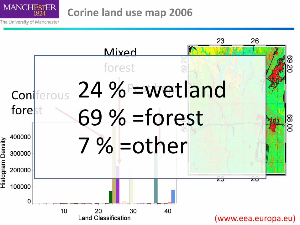
Corine land use map 2006

Coniferous forest

Peat bogs

Mixed forest

(www.eea.europa.eu)

Corine land use map 2006

Coniferous forest

Peat bogs

Mixed forest

(www.eea.europa.eu)

24 % =wetland 69 % =forest 7 % =other

Comparison with ground based fluxes

Scale chamber fluxes using the land types within the aircraft footprint.

IDL Exercise

• Go to (or navigate to via www.faam.ac.uk):

http://www.faam.ac.uk/index.php/flying-calendar/icalrepeat.detail/2015/05/12/9880/-/b905-b906-gauge-flight Read the “sortie briefs”

Photo: Nicola Warwick