INTERPRETATION AND ESTIMATION OF DEFAULT · PDF fileIn the target portfolio, the credit risk...

INTERPRETATION AND ESTIMATION

OF DEFAULT CORRELATIONS

Petit Dejeuner de la Finance

Maison des Polytechniciens - Frontieres en Finance,29 Septembre 2004

P. Demey & T. Roncalli

Joint work with D. Kurtz, J-F. Jouanin, A. Quillaud & C. Roget

Groupe de Recherche Operationnelle

Credit Agricole SA

http://gro.creditlyonnais.fr

Agenda

• Motivations

• 1st Case : Default Correlations and Loss distribution of a Credit

Book

1. Raroc and credit pricing

2. Credit portfolio management

3. Definition of default correlations

4. MLE of default correlations

• 2nd Case : Default Correlations and Credit Basket

Pricing/Hedging

1. Duality between factor models and copula models

2. Default correlations and spread jumps

3. Trac-X implied correlation

4. Implications for CDO pricing

Interpretation and Estimation of Default Correlations 1

1 Motivations

Correlations = Parameter of the multivariate Normal distribution /

Linear dependence between gaussian random variables

⇒ The second point of view is the reference in finance (regression,

factor analysis, etc.)

In asset management, correlations are used to represent the

dependence between returns.

Objective: computing risk/return of portfolios.

⇒ Correlation = a good tool for credit risk modelling ?

Interpretation and Estimation of Default CorrelationsMotivations 1-1

Our point of view = Correlation is a mathematical tool to define the

loss of credit portfolios (CreditRisk+).

Default correlation 6= dependence between default times (KMV,

CreditMetrics).

⇒ Credit Portfolio Management = Loss distribution of a portfolio

(Credit VaR, Risk Contribution, Stress Testing, etc.)

⇒ Credit Derivatives Pricing/Hedging = Loss distribution of a

tranche & Spread dynamics

Interpretation and Estimation of Default CorrelationsMotivations 1-2

2 Default Correlations and Loss distribution of a

Credit Book

Interpretation and Estimation of Default CorrelationsDefault Correlations and Loss distribution of a Credit Book 2-1

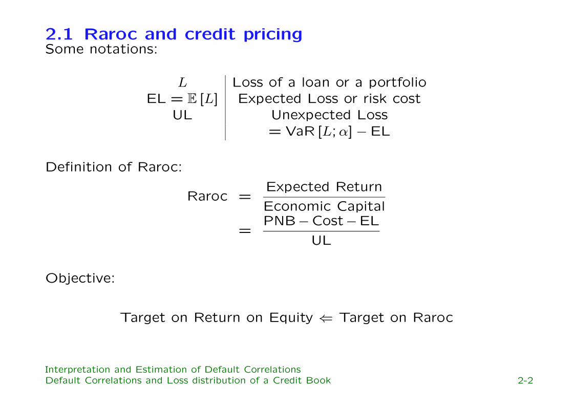
2.1 Raroc and credit pricingSome notations:

L Loss of a loan or a portfolioEL = E [L] Expected Loss or risk cost

UL Unexpected Loss= VaR [L;α] − EL

Definition of Raroc:

Raroc =Expected Return

Economic Capital

=PNB−Cost−EL

UL

Objective:

Target on Return on Equity ⇐ Target on Raroc


2.1.1 Ex-Ante Raroc of a loan

Economic Capital = Risk contribution of the loan to the total risk of

the portfolio

Raroc =Expected Return

Risk Contribution of the loan

Problems: What is the target portfolio of the bank ? Given this

portfolio, how to calibrate the parameters of the Raroc model ? How

to approximate the risk contribution when the credit is well modelled

(ex-ante raroc) ?


2.1.2 An example with an infinitely fine-grained portfolio

and a one factor modelLet UL = VaR [L;α] − EL. If the portfolio is infinitely fine-grained, we

have RCi = E [Li | L = EL+UL] − E [Li]. We consider the following

proxy UL? = k × σ (L). Because we have:

σ (L) =∑

i

σ (Li)cov (L, Li)

σ (L)σ (Li)=∑

i

fi × σ (Li)

we deduce that a proxy of the risk contribution is

RC?i = k × fi × σ (Li). fi is called the diversification factor, because it

depends on the dependence structure of the portfolio. In the case of

one-factor model and an homogeneous portfolio, we obtain:

f =

√

√

√

√

√

C (PD,PD; ρ) − PD2

σ2[LGD]E2[LGD]

PD+(

PD−PD2)

⇒ f depends on the default correlation ρ.


2.2 Credit Portfolio Management⇒ Moving the original portfolio to obtain the target portfolio

• the original portfolio without management is generally

concentrated (either at a name, industry or geography level, etc.)

• the target portfolio is generally an infinitely fine-grained portfolio

which has some other good properties (= optimise the capital)

Dis-investment / Re-investment

• Single-name hedges (CDS) / Multi-name hedges (F2D, CDO)

• Securitisations (CBO)

• Investment opportunities (CDS / CDO)

⇒ CPM needs default correlations.


2.3 Definition of default correlations

• Default time correlation ρ (τ1, τ2)

• Default event correlations ρ (1 {τ1 ≤ t1} , 1 {τ2 ≤ t2})• Spread jumps s1 (t1 | τ2 = t2, τ1 ≥ t2)

• Asset / Equity correlations

⇒ How to calibrate correlations needed by CPM ?

In the target portfolio, the credit risk is principally a risk on default

rates.

probability of default ⇔ mean of default rates

default correlations ⇔ volatility of default rates


2.4 Data

• History of annual default rates by risk class

• Risk classes are typically industrial sectors, rating grades,

geographical zones, ...

For example : S&P provides this data, between 1980 and 2002 by

industrial sector and by rating.


2.5 The model

• Merton model : obligor n defaults if and only if Zn ≤ Bn.

• The latent variable Zn is gaussian

• Homogeneity of risk classes : Bn = Bc

• Within a given class of risk the correlation between two firms is

constant, that is:

ρm,n = ρc, ∀m, n ∈ c

• Given any pair of risk classes (c, d) there is a unique correlation

between any couple of firms (m, n) belonging to each class, that

is:

ρm,n = ρc,d, ∀m ∈ c, n ∈ d


Let’s define

Σ =

ρ1 ρ1,2 . . . ρ1,Cρ2,1 ρ2

. . . ...... . . . . . . ρC−1,C

ρC,1 . . . ρC,C−1 ρC

then we can rewrite Zn as a linear function of F factors Xf (with

A>A = Σ)

Zn =F∑

f=1

Af,cXf +√

1 − ρcεn, n ∈ c

2.6 MLE of default correlations

The number of default in risk class Dc | X = x ∼ B (nct;Pc (x)

)

.

The default probability conditionally to the factors X is:

Pc (x) = Φ

Bc −∑Ff=1 Af,cxf√1 − ρc

The unconditional log-likelihood is then:

`t (θ) = ln∫

· · ·∫

RF

C∏

c=1

Binc,t (x) dΦ (x)

with:

Binc,t (x) =(nc

t

dct

)

Pc (x)dct (1 − Pc (x))nc

t−dct

⇒ The loglikelihood is not tractable (in particular when C increases),

due to the multi-dimensional integration.


2.7 Constrained Model

Σ =

ρ1 ρ . . . ρρ ρ2

. . . ...... . . . . . . ρρ . . . ρ ρC

Zn =√

ρX +√

ρc − ρXc +√

1 − ρcεn

Interpretation : Zn is explained by a common factor X and by a

specific factor Xc depending on the risk class.

Why : robustness of estimation; this assumption seems intuitive

Pc (x, xc) = Φ

(

Bc −√ρx −√

ρc − ρxc√1 − ρc

)


2.7.1 Binomial MLE

The conditional likelihood is first computed and then integrated

successively on the distribution of each sectorial factor and on the

distribution of the common factor:

`t (θ) = ln∫

R

C∏

c=1

∫

R

Binc,t (x, xc) dΦ (xc)

dΦ (x)

This is the ’binomial’ MLE.


2.7.2 Asymptotic MLE

Let µct =

dct

nctbe the default rate at time t in class c.

µct | X = x, Xc = xc → P (x, xc)

The loglikelihood function is then:

`t (θ) = ln∫ 1

0

C∏

c=1

φ (f (y))

√1 − ρc√ρc − ρ

1

φ(

Φ−1(

µct

)

) dy

with:

f (y) =Bc −√

1 − ρcΦ−1 (µc

t)−√

ρΦ−1 (y)√ρc − ρ


2.8 Monte Carlo simulationsSingle-factor T = 20 years, number of firms nt = N = 200,

homogeneous class (PD = 200 bp), ρ = 25%

• MLE1: full information estimator (B = Φ−1 (PD) is known)

• MLE2: limited information estimator (B is estimated)

Asymptotic BinomialStatistics (in %) MLE1 MLE2 MLE1 MLE2

mean 23.7 22.5 25.2 23.6std error 5.8 7.2 7.6 8.5

Statistics of the estimates (PD = 200 bp)

⇒ Bias for Asymptotic estimators

⇒ Downward bias for MLE2

⇒ Standard error is important


Impact of N on binomial MLE

Impact of N on asymptotic MLE

Two risk classes

Σ =

(

ρ1 ρρ ρ2

)

=

(

20% 7%7% 10%

)

Statistics Asymptotic Binomial(in %) ρ1 ρ2 ρ ρ1 ρ2 ρmean 19.9 12.9 6.5 19.9 10.7 7.5std error 4.8 3.1 3.1 6.4 4.3 3.7Statistics of the estimates (PD = 200 bp)

Remark 1 The bias seems lower than in the one risk class

experiment.

2.9 Estimation using S&P data

two-factor Single-factorNc µc Asymp. Bin. Asymp. Bin.

Aerospace / Automobile 301 2.08% 13.3% 13.9% 13.7% 11.6%Consumer / Service sector 355 2.37% 12.2% 10.6% 12.2% 8.9%Energy / Natural ressources 177 2.10% 23.2% 25.5% 16.2% 14.5%

Financial institutions 424 0.57% 17.0% 16.4% 12.0% 9.5%Forest / Building products 282 1.90% 18.1% 18.8% 28.6% 31.5%

Health 135 1.27% 12.9% 10.6% 13.1% 13.2%High technology 131 1.66% 15.0% 16.4% 12.9% 10.6%

Insurance 166 0.61% 26.3% 34.3% 13.6% 17.8%Leisure time / Media 232 3.01% 13.8% 9.4% 17.2% 12.0%

Real estate 133 1.01% 43.2% 52.4% 48.7% 53.0%Telecoms 100 1.91% 22.9% 29.1% 27.0% 34.0%

Transportation 146 2.02% 17.7% 11.1% 12.8% 10.4%Utilities 206 0.43% 14.4% 18.7% 10.4% 17.5%

Inter-sector 7.2% 9.4% X X


Conclusion

• we extend the study of Gordy and Heitfield (2002)

• we apply our methodology to S&P data

• there is a downward bias that one could try to correct

Application to Stress-Testing

⇒ Pillar II.


3 Default Correlations and Credit Basket

Pricing/Hedging

Interpretation and Estimation of Default CorrelationsDefault Correlations and Credit Basket Pricing/Hedging 3-1

3.1 Duality between factor models and copula models

Let Zi =√

ρX +√

1 − ρεi be a latent variable with X the common

factor and εi the specific factor. We have

Di (t) = 1 ⇔ Zi < Bi = Φ−1 (PDi (t))

Let Σ = C (ρ) be the constant correlation matrix. We have

S (t1, . . . , tI) = Pr {τ1 > t1, . . . , τI > tI}= Pr

{

Z1 > Φ−1 (PD1 (t1)) , . . . , ZI > Φ−1 (PDI (tI))}

= C (1 − PD1 (t1) , . . . ,1 − PDI (tI) ;Σ)

= C (S1 (t1) , . . . ,SI (tI) ;Σ)

where C is the Normal copula.

Remark 2 Let τ1 et τ2 be two default times with the joint survival

function S (t1, t2) = C (S1 (t1) ,S2 (t2)). We have

S1 (t | τ2 = t?) = ∂2C (S1 (t) ,S2 (t?)). If C 6= C⊥, default probability of

one firm changes when the other has defaulted.


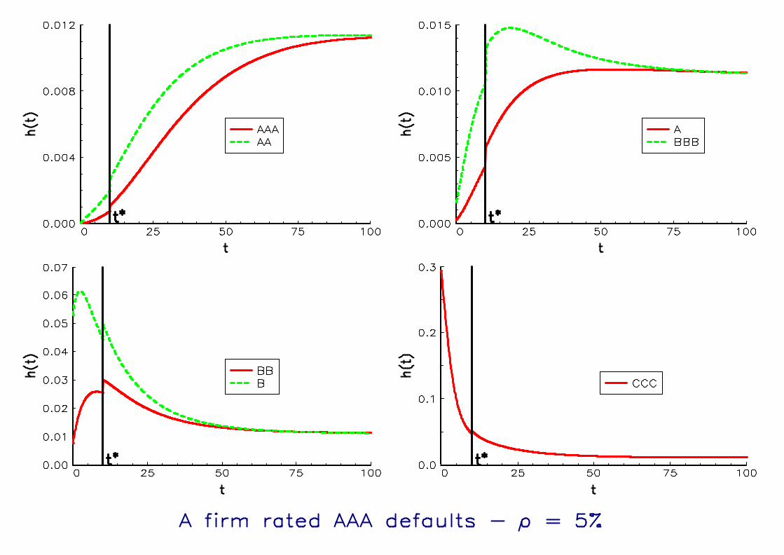
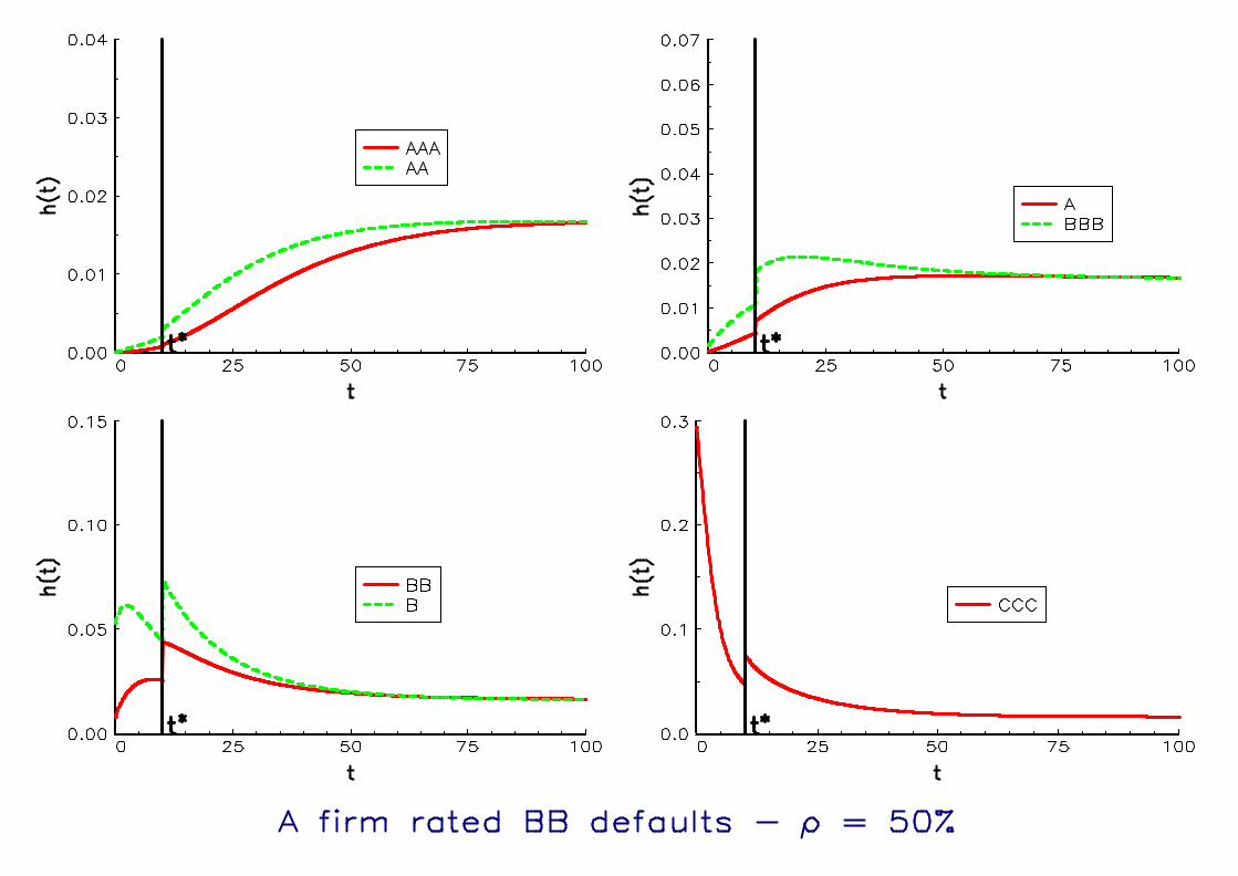
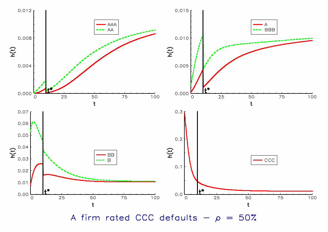
Example 1 The next figures show jumps of the hazard function

λ (t) = f (t) /S (t) of the annual S&P transition matrix. With a

Normal copula and Σ = CI (ρ), we have

S1(

t | τ2 = t?)

= Φ

Φ−1 (S1 (t)) − ρΦ−1 (S2 (t?))√

1 − ρ2

3.2 Default correlations and spread jumps

We assume an exponential default model with intensity λ. Let s and

R be the spread of the CDS and the recovery rate. We have

s = λ (1 − R)

It comes that the default probability is

PD(t) = 1 − exp

(

− s

1 − Rt

)

The conditional probability of the first name given that the second

name has defaulted at time t? is then

PD1(

t | τ2 = t?)

= ∂2C(

PD1 (t) ,PD2(

t?))

(t ≥ t?)

we deduce that the spread of the first name after the default of the

second name becomes

s1(

t | τ2 = t?, τ1 ≥ t?)

= −(1 − R1)

(t − t?)ln(

1 − PD1(

t | τ2 = t?, τ1 ≥ t?))


Correlation implied to Ahold default

Start Wide Jump

Recovery 28/10/2002 28/02/2003 Normal T4AHOLD 40% 235 1205 970CASINO 40% 235 152 -83 -8 -48SAINSBURY 40% 48 95 47 12 -31CARREFOUR 40% 60 47 -13 -4 -52KROGER 40% 127,5 108 -19,5 -3 -47SAFEWAY 40% 66,5 145 78,5 15 -27

Correlation implied

Start Wide Jump

Recovery 20/02/2003 28/02/2003 Normal T4AHOLD 40% 195 1205 1010CASINO 40% 135 160 25 -7 -79SAINSBURY 40% 68 95 27 3 -76CARREFOUR 40% 43 47 4 1 -80KROGER 40% 90 95 5 1 -78SAFEWAY 40% 195 145 -50 -3 -78

Correlation implied


Correlation implied to Worldcom default

Start Wide Jump

Recovery 05/07/2001 01/05/2002 Normal T4WORLDCOM 15% 165 1700 1535TELECOMI 15% 165 130 -35 -5 -41TELEFONI 15% 95 80 -15 -3 -43BELLSOUT 15% 47 75 28 9 -31BRITELEC 15% 105 105 0 0 -39MOTOROLA 15% 285 300 15 1 -29ATTCORP 15% 110 600 490 45 19TELECOM 15% 185 345 160 15 -16

Correlation implied

Correlation implied to TXU Corp. default

Start Wide Jump

Recovery 13/08/2002 10/10/2002 Normal T4TXU Corp. 40% 450 1250 800SEMPRA 40% 275 400 125 7 -33DUKEENER 40% 170 225 55 5 -39VIVENENV 40% 170 152,5 -17,5 -2 -48SUEZ 40% 105 130 25 4 -43AMELECPO 40% 380 925 545 20 -15RWEAG 40% 67 98 31 6 -41ENEL 40% 68 87 19 4 -44

Correlation implied


3.3 Trac-X implied correlationModel : Zi = βX +

√

1 − β2εi. ⇒ β =√

ρ.

Expectation of losses (5Y maturity)

Value of the floating leg (5Y maturity)

Implied correlation

Attachment points: 0 = A0 < A1 < ... < AM ≤ 1

Marked spread: s(Ai−1, Ai)

obs for the tranche [Ai−1, Ai]

The implied correlation for the tranche [Ai−1, Ai] verify:

∀i 6= 1, s(Ai−1, Ai, ρ(Ai−1, Ai)) = s(Ai−1, Ai)obs,

(correction for the equity tranche because of upfront payment)


0

0,1

0,2

0,3

0,4

0,5

0,6

0,7

0,8

0,9

1

0 10 20 30 40 50 60 70 80 90correlation

pourcentage de pertes tranche equity:0%->3%

tranche mezanine:3%->12%

tranche senior:12%->100%

0

0,5

1

1,5

2

2,5

3

3,5

0 10 20 30 40 50 60 70 80 90

correlation (%)

Jambe Variable

tranche equity: 0%->3%

tranche mezzanin: 3%->12%

tranche senior:12%->100%

Example: Trac-X Euro 02/06/2004.

A B Upfront payment Running spread (bp)0% 3% 34% 5003% 6% 2796% 9% 1149% 12% 5812% 22% 23

Implied correlation of Trac-X

Loss distribution for the second tranche

Base correlation of Trac-X

Implied correlation of Trac-X (T9 copula)


0

0,1

0,2

0,3

0,4

0,5

0,6

0,7

0,8

0%->3% 3%->6% 6%->9% 9%->12% 12%->22%

tranches

correlation implicite

0

0,1

0,2

0,3

0,4

0,5

0,6

0,7

0,8

0,9

0 0,2 0,4 0,6 0,8 1

% pertes sur la tranche

probabilité corrélation implicite=0,04

corrélation implicite=0,75

0

0,1

0,2

0,3

0,4

0,5

0,6

0,7

0,8

0 3 6 9 12 15 18 21 24

point d'attachement haut (%)

base correlation

0

0,1

0,2

0,3

0,4

0,5

0,6

0,7

0,8

0,9

0->3% 3->6% 6->9% 9->12% 12->22%

tranches

correlation implicite

Gaussian factors with three types of names (spread = 50 bp, 150 bp

and 250 bp).

Three structures of correlation :

Σ1 =

1 0.32 0.32

0.32 1 0.32

0.32 0.32 1

, Σ2 =

1 0.1 × 0.3 0.1 × 0.50.1 × 0.3 1 0.3 × 0.50.1 × 0.5 0.3 × 0.5 1

Σ3 =

1 0.5 × 0.3 0.1 × 0.50.5 × 0.3 1 0.3 × 0.10.1 × 0.5 0.3 × 0.1 1


0

0,05

0,1

0,15

0,2

0,25

0,3

0->3% 3->6% 6->9% 9->12% 12->22% 22->100%

Tranches

correlation implicite Betas corrélés

Betas anticorrélés

Betas=0,3

3.4 Implications for CDO pricing

Implied correlation = not useful for CDO pricing.

Implied correlation of CDO 6= Implied correlation of spread of two

equity indices

A new dimension = TRAC-X PORTFOLIO.

What is the meaning of implied correlation ?

⇒ the mathematical root of an equation


INTERPRETATION AND ESTIMATION OF DEFAULT · PDF fileIn the target portfolio, the credit risk...

Documents

Transcript of INTERPRETATION AND ESTIMATION OF DEFAULT · PDF fileIn the target portfolio, the credit risk...