Interpolation Methods for Curve Construction · Interpolation Methods for Curve Construction...

Interpolation Methods for CurveConstruction

PATRICK S. HAGAN* & GRAEME WEST**

*Bloomberg, LP, 499 Park Avenue, New York, NY 10022, USA, **Programme in Advanced Mathematics of

Finance, School of Computational & Applied Mathematics, University of the Witwatersrand, Private Bag 3,

Wits 2050, South Africa

(Received 30 November 2004; in revised form 6 July 2005)

ABSTRACT This paper surveys a wide selection of the interpolation algorithms that are in use infinancial markets for construction of curves such as forward curves, basis curves, and mostimportantly, yield curves. In the case of yield curves the issue of bootstrapping is reviewed andhow the interpolation algorithm should be intimately connected to the bootstrap itself is discussed.The criterion for inclusion in this survey is that the method has been implemented by a softwarevendor (or indeed an inhouse developer) as a viable option for yield curve interpolation. As will beseen, many of these methods suffer from problems: they posit unreasonable expections, or are noteven necessarily arbitrage free. Moreover, many methods lead one to derive hedging strategiesthat are not intuitively reasonable. In the last sections, two new interpolation methods (themonotone convex method and the minimal method) are introduced, which it is believed overcomemany of the problems highlighted with the other methods discussed in the earlier sections.

KEY WORDS: Yield curve, interpolation, bootstrap

Curve Fitting

There is a need to value all instruments consistently within a single valuation

framework. For this we need a risk-free yield curve which will be a continuous zero

curve (because this is the standard format, for all option pricing formulae). Thus, a

yield curve is a function r5r(t), where a single payment investment for time t will

earn a continuous rate r5r(t), that is, a payment of 1 at initiation will be redeemed

by a payment of exp(r(t)t) at time t.

As explained in Zangari (1977) and Lin (2002) term structure estimation methods

can be classified into two groups: theoretical and empirical. Theoretical term

structure methods typically posit an explicit structure for a variable known as the

short rate of interest, whose value depends on a set of parameters that might be

Correspondence Address: Graeme West, Programme in Advanced Mathematics of Finance, School of

Computational & Applied Mathematics, University of the Witwatersrand, Private Bag 3, Wits 2050, South

Africa. Tel.: +27-11-4472901; Email: [email protected]

Applied Mathematical Finance,

Vol. 13, No. 2, 89–129, June 2006

1350-486X Print/1466-4313 Online/06/020089–41 # 2006 Taylor & Francis

DOI: 10.1080/13504860500396032

determined using statistical analysis of market variables. Early examples of

theoretical methods include Vasicek (1977) and Cox et al. (1985). From such a

method the yield curve can be derived. Because the theoretical method is

parsimonious, the yield curve will fall into one of a few basic categories in terms

of shape. In some circumstances, negative rates are possible.

Empirical methods are available to compute spot interest rates. Unlike the

theoretical methods, the empirical methods are independent of any model or theory

of the term structure. Whereas the theoretical methods attempt to explain typical

features of the term structure, which may include how the term structure evolves

through time, the empirical methods merely try to find a close representation of the

term structure at any point in time, given some observed interest rate data.

Later developments, in particular the approach of Hull and White (1990), allowed

the use of a empirically determined yield curve in a theoretical model. Furthermore,

the classification scheme of Heath et al. (1990) takes as input the same empirically

determined yield curve. Thus, while the practitioner has several choices for the

theoretical model that will govern their evolution of the yield curve, and hence

govern their pricing of derivative products, they will almost certainly have as starting

point an empirically determined yield curve. This document is concerned with that

task of determining the yield curve, a process typically called bootstrapping. In fact,

our treatment is slightly more general, as it covers the construction of spread curves,

forward curves, etc. as well.

As explained in several sources, for example Ron (2000), there is no single correct

way to complete the term structure of a yield curve from a set of rates. It is desired

that the derived yield curve should be smooth, but there must not be over-

smoothing, as this might cause the elimination of valuable market pricing

information. It may or may not be a criterion that all inputs to the yield curve

should price back exactly after the construction of that curve, although we certainly

prefer an approach where there are fewer inputs and hence this perfect replication is

feasible. We will typically be following this approach, although the issue of error

minimization when there is a large set of inputs will be mentioned later. Certainly

this approach is completely feasible when bootstrapping a swap curve, it may or may

not be feasible when bootstrapping a bond curve, this will depend on the number of

liquid bonds available in the market. Even when we require that the curve perfectly

replicates the price of the input instruments, the yield curve is not constructed

uniquely; we need to select an interpolation method with which to build the curve.

In this paper we survey a wide, but not exhaustive, selection of the interpolation

methods that are in use in financial markets and their systems. In later sections we

introduce two new interpolation methods, which we believe overcome many of the

problems highlighted with other methods that have been discussed in the earlier sections.

Desirable Features of an Interpolation Scheme

The criteria to use in judging a curve construction and its interpolation method that

we will consider are:

(1) In the case that we have a small set of instruments with which we are building

an exact empirical curve, does this indeed occur? In the case that we are using a

90 P. S. Hagan and G. West

large set of instruments, does the algorithm to find the best fit curve converge

sufficiently rapidly, and is the degree of error in the created curve sufficiently

small?

(2) In the case of yield curves, how good do the forward rates look? These are

usually taken to be the 1 month or 3 month forward rates, but these are

virtually the same as the instantaneous rates. We will want to have positivity

and continuity of the forwards. It is required that forwards be positive to avoid

arbitrage, while continuity is required as the pricing of interest-sensitive

instruments is sensitive to the stability of forward rates. As pointed out in

McCulloch & Kochin (2000), ‘a discontinuous forward curve implies either

implausible expectations about future short-term interest rates, or implausible

expectations about holding period returns’. Thus, such an interpolation

method should probably be avoided, especially when pricing derivatives whose

value is dependent upon such forward values.

(3) How local is the interpolation method? If an input is changed, does the

interpolation function only change nearby, with no or minor spill-over

elsewhere, or can the changes elsewhere be material?

(4) Are the forwards not only continuous, but also stable? We can quantify the

degree of stability by looking for the maximum basis point change in the

forward curve given some basis point change (up or down) in one of the inputs.

Many of the simpler methods can have this quantity determined exactly, for

others we can only derive estimates.

(5) How local are hedges? Suppose we deal with an interest rate derivative of a

particular tenor. We assign a set of admissible hedging instruments, for

example, in the case of a swap curve, we might (even should) decree that the

admissible hedging instruments are exactly those instruments that were used to

bootstrap the yield curve. Does most of the delta risk get assigned to the

hedging instruments that have maturities close to the given tenors, or does a

material amount leak into other regions of the curve?

We will discuss criteria (1) and (2) as we proceed with each method that we

analyse. Criteria (3), (4) and (5) will be discussed much later.

In most cases we have the rates r1, r2, …, rn at the nodes t1, t2, …, tn and need to

determine the rate r(t) where t is not necessarily one of the ti. Occasionally we will

have the forward rates rather than the rates themselves, and are required to perform

the interpolation on these. In these cases, we may wish to recover the rates using the

relationship f tð Þ~ LLt r tð Þt.

For any t =[ t1, tn½ �, the value of r(t) or f(t) will be that rate found at the nearer of

t1 or tn.

Note that the forward is positive if and only if the capitalization function is

increasing, equivalently, r(t)t is increasing.

Interpolation and Bootstrap of Yield Curves – not two Separate Processes

As has been mentioned, many interpolation methods for curve construction are

available. What needs to be stressed is that in the case of bootstrapping yield curves,

Interpolation Methods for Curve Construction 91

the interpolation method is intimately connected to the bootstrap, as the bootstrap

proceeds with incomplete information. This information is ‘completed’ (in a non-

unique way) using the interpolation scheme.

Swap Curves

Let us first consider swap curves. Suppose a swap makes the fixed payments at time

t1, t2, …, tn; time is measured in years. As explained in Hull (2002, Section 6.4), a

swap just issued at par can be valued by

Rn

Xn

i~1

aiZ tið ÞzZ tnð Þ~1 ð1Þ

where Rn is the par swap rate, and ai is the time in years from ti21 to ti, calculated

with the relevant day count convention. In the theory, Rn is now solved for, as

Rn~1{Z tnð ÞPni~1 aiZ tið Þ

ð2Þ

Alternatively, we can inductively suppose that Z(ti) is known for i51, 2, …, n21,

and Rn is known, to get

Z tnð Þ~1{Rn

Pn{1i~1 aiZ tið Þ

1zRnan

ð3Þ

At first blush, use of (3) assumes that inputs to the curve are available for all

standard tenors1 to maturity. This is typically not the case. For example, in

constructing a swap curve, we might use deposit rates in the very short term, forward

rate agreements or futures in the short to medium term, and swap rates in the longer

term. Typically, the FRA or futures rates will be available for calculation of the

relevant rates for all three-month tenors out to say two years.

The use of futures and FRAs will pose no difficulty. One applies a standard

convexity adjustment to futures prices to get an equivalent FRA rate. This convexity

adjustment will depend on some time and volatility parameters, but not on the yield

curve itself. However, the swap rates may only be available in say 2, 3, 4, up to 10

year tenors. What to do about tenors which are not in whole number of years away?

Even worse, the swap rates may only be available in say 2, 3, 4, 5 and 10 year tenors,

with the 6 to 9 year tenors insufficiently liquid to use with confidence. Thus, lack of

liquidity can reduce our information set dramatically.

One approach now advocated in some sources is to interpolate (linearly, say) the

input swap rates to the expiries which are not quoted, and then proceed with a

complete information set. However, this decouples the interpolation procedure from

the bootstrap procedure, even if the chosen interpolation method here is the same as

the interpolation method that will be used to find rates at points which are not nodes

after the bootstrap is completed. Rather, we rewrite (3) as

rn~{1

tn

ln1{Rn

Pn{1j~1 ajZ t, tj

� �

1zRnan

" #ð4Þ


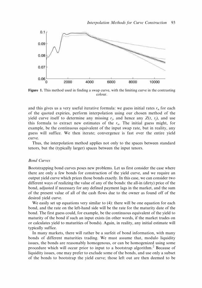
and this gives us a very useful iterative formula: we guess initial rates rn for each

of the quoted expiries, perform interpolation using our chosen method of the

yield curve itself to determine any missing rj, and hence any Z(t, tj), and use

this formula to extract new estimates of the rn. The initial guess might, for

example, be the continuous equivalent of the input swap rate, but in reality, any

guess will suffice. We then iterate; convergence is fast over the entire yield

curve.

Thus, the interpolation method applies not only to the spaces between standard

tenors, but the (typically larger) spaces between the input tenors.

Bond Curves

Bootstrapping bond curves poses new problems. Let us first consider the case where

there are only a few bonds for construction of the yield curve, and we require an

output yield curve which prices those bonds exactly. In this case, we can consider two

different ways of realizing the value of any of the bonds: the all-in (dirty) price of the

bond, adjusted if necessary for any defined payment lags in the market, and the sum

of the present value of all of the cash flows due to the owner as found off of the

desired yield curve.

We easily set up equations very similar to (4): there will be one equation for each

bond, and the rate on the left-hand side will be the rate for the maturity date of the

bond. The first guess could, for example, be the continuous equivalent of the yield to

maturity of the bond if such an input exists (in other words, if the market trades on

or calculates yield to maturities of bonds). Again, in reality, any initial estimate will

typically suffice.

In many markets, there will rather be a surfeit of bond information, with many

bonds of different maturities trading. We must assume that, modulo liquidity

issues, the bonds are reasonably homogenous, or can be homogenized using some

procedure which will occur prior to input to a bootstrap algorithm.2 Because of

liquidity issues, one may prefer to exclude some of the bonds, and use only a subset

of the bonds to bootstrap the yield curve; those left out are then deemed to be

Figure 1. This method used in finding a swap curve, with the limiting curve in the contrastingcolour.


marked to market at the price one obtains by stripping them off the yield curve,

rather than the illiquid (and hence by now ‘erroneous’) last price at which they

traded.

A key issue is to decide on how many bonds to include as bona fide inputs to the

bootstrap. To exclude too many runs the risk of excluding market information

which is actually meaningful, on the other hand, including too many could result

in a yield curve that is implausible, a yield curve that admits arbitrage, or a

bootstrap algorithm that fails to converge. In this case, we need to consider

constructing a yield curve that ‘does as good a job as possible’ in recovering the

prices of the inputs.

In this case, what needs to be done can easily be understood; we will not deal with

the specifics here, they will involve some multi-dimensional minimization problem.

One needs to fix some set of node points, for example, they could be the maturity

dates of those bonds that are deemed to be the most important, or could be the same

nodes as exist in the swap curve, for example. One then postulates values of the yield

curve at each of those node points, and completes the yield curve by using the chosen

interpolation method. We can then calculate the value of each bond as stripped off

this curve, versus the value that it is trading at in the market. The error (typically

squared, and possibly weighted in order to attach more importance to some bonds

than to others) is then summed across all the bonds. The values of the curve at the

node points are perturbed, using some optimisation routine, to minimise this

summed error.

We now go on to consider a variety of interpolation methods.

Simple Interpolation Methods

Suppose we are given some t g (t1, tn) which is not equal to any of the ti. First we

determine i such that ti , t , ti+1.

The methods discussed in this section only use the rates ri and ri+1 in order to

estimate r(t). Typically, the methods can be formulated as implicitly linear

interpolation on the discount function, spot function, or some other transformation,

such as the logarithm of the discount or spot function. Other methods will require

some property of the forward function, for example, piecewise constant. Possible

methods are:

Linear on Discount Factors

Let d(t) 5 exp(2r(t)t) be the discount function, with di and di+1 having their obvious

meanings. Then for this method we have

d tð Þ~ t{ti

tiz1{ti

diz1ztiz1{t

tiz1{ti

di

and so

r tð Þ~ {1

tln

t{ti

tiz1{ti

diz1ztiz1{t

tiz1{ti

di

� �ð5Þ


For the forward function, we calculate

f tð Þ~ LLt

r tð Þt

~{

1

tiz1{ti

diz1{1

tiz1{ti

di

t{ti

tiz1{ti

diz1ztiz1{t

tiz1{ti

di

~di{diz1

t{tið Þdiz1z tiz1{tð Þdi

which shows that the forward is not continuous (by the time t reaches ti+1, the input

from ti has not been ‘forgotten’).

Linear on Spot Rates

r tð Þ~ t{ti

tiz1{ti

riz1ztiz1{t

tiz1{ti

ri ð6Þ

In this case clearly

f tð Þ~ 2t{ti

tiz1{ti

riz1ztiz1{2t

tiz1{ti

ri ð7Þ

and, as before, the forward rates are not continuous.

Raw Interpolation

This method is linear on the logarithm of discount factors, and as we shall see,

corresponds to piecewise constant forward curves. To a good approximation, any

forward curve that has the same area between each node would work. This means

that if a piecewise linear approximation starts too high, it has to go too low to

average to the right value, but then it starts the next interval too low and has to go

too high to average to the right value. This method is very stable, is trivial to

implement, and is usually a base method one implements in a system before any

others. One can often find mistakes in fancier methods by comparing the raw

method with the more sophisticated method.

Since the instantaneous forward curve is f tð Þ~ LLt r tð Þt, the interpolating function

for the yield curve is r tð Þ~Kz Ct . Given the two endpoints, this solves as

f tð Þ : ~K~riz1tiz1{riti

tiz1{ti

C~ri{riz1ð Þtitiz1

tiz1{ti

and after some manipulation, we get

r tð Þ~ t{ti

tiz1{ti

tiz1

triz1z

tiz1{t

tiz1{ti

ti

tri

ð8Þ


Note that this method is occasionally called exponential interpolation, as it involves

exponential interpolation of the discount factors i.e.

d tð Þ~d

t{titiz1{ti

iz1 d

tiz1{t

tiz1{ti

i

This is equivalent to linear interpolation of the logarithm of the discount factors,

and this should not be a surprise: one always has that

f tð Þ~{LLt

ln d tð Þ ð9Þ

and so the constant forward model is easily seen to be equivalent to this type of

linear interpolation.

Linear on the Logarithm of Rates

This method is called log-linear interpolation or even exponential interpolation.

If

ln r tð Þ~ t{ti

tiz1{ti

ln riz1ztiz1{t

tiz1{ti

ln ri

then

r tð Þ~r

t{titiz1{ti

iz1 r

tiz1{t

tiz1{ti

i ð10Þ

Since

ln r tð Þt~ t{ti

tiz1{ti

ln riz1ztiz1{t

tiz1{ti

ln rizln t

we have

1

r tð Þt f tð Þ~ 1

tiz1{ti

lnriz1

ri

z1

t

and so

f tð Þ~r tð Þ t

tiz1{ti

lnriz1

ri

z1

� �ð11Þ

Remarkably, this method is quite popular, being provided as one of the default

methods by many software vendors. However, it clear from (11) that this method

does not guarantee positive forward rates. As a trivial (not necessarily practicable)

example, if we have a two-point curve, with nodes (1,6%) and (30,2%) then the

forward rates are negative from about the 26th year.

All these simple methods have continuity difficulties associated with them. Thus,

they should not be used for anything but naive interpolation of yield curves,

after which criteria such as rate smoothness, forward rate smoothness etc. are

important.


Piecewise Linear Continuous Forwards

Let us quickly consider this method; just as quickly we will reject it.

When considering this method we find that the forward curve exhibits enormous

zig-zag instability. As a simple example, suppose the continuous rates for a yield

curve are specified at all whole number terms, with r(t) 5 r for t(T, some specified

T, and r(t) 5 r+e for t > T + 1. Then f(t) 5 r for t(T. The discrete forward from T to

T+1 is r + e(1+T). Hence f(T+1) 5 r + 2e(1+T). Then f(T+2) 5 r22eT, and the pattern

repeats itself for odd and even increments from T.

Cubic Splines

As before, suppose t1, t2, …, tn and r1, r2, …, rn, ri:5r(ti) are known. To complete a

cubic spline, we desire coefficients (ai, bi, ci, di) for 1(i(n21. Given these

coefficients, the function value at any term t will be

r tð Þ~aizbi t{tið Þzci t{tið Þ2zdi t{tið Þ3 tiƒtƒtiz1 ð12Þ

Note that

r0 tð Þ~biz2ci t{tið Þz3di t{tið Þ2 tivtvtiz1

r00 tð Þ~2ciz6di t{tið Þ tivtvtiz1

r000 tð Þ~6di tivtvtiz1

Let hi 5 ti+12ti throughout. The constraints common to all methods will be

N the interpolating function indeed meets the given data, so ai 5 ri for i 5 1, 2, …,

n21 and an{1zbn{1hn{1zcn{1h2n{1zdn{1h3

n{1~rn : ~an;

N the entire interpolating function is continuous, so aizbihizcih2i zdih

3i ~ aiz1 for

i 51, 2, …, n22;

N the entire function is differentiable, so biz2cihiz3dih2i ~ biz1 for i 5 1, 2, …,

n22.

This is a system of 3n24 equations in 4n24 unknowns. Thus there are n linear

constraints still to be specified.

A fundamental reason for requiring differentiability of the interpolating

function is that then the forward function f tð Þ~ LLt r tð Þt is continuous. We clearly

have

f tð Þ~aizbi 2t{tið Þzci t{tið Þ 3t{tið Þzdi t{tið Þ2 4t{tið Þ tiƒtƒtiz1 ð13Þ

Let us define

bn : ~bn{1z2cn{1hn{1z3dn{1h2n{1 ð14Þ

so that bn is the derivative of the interpolating function at the right hand endpoint. In

the most general case (de Boor 1978, 2001, Chapter IV), the specification of the

remaining n linear constraints is equivalent to specifying b1, b2, …, bn (as any n

additional conditions will do, assuming there is no redundancy - the point in de


Boor, 1978, 2001, is that such a view can be an aid to classification). In particular, if

we take this approach, defining b1, b2, …, bn, then c1, c2, …, cn21 and d1, d2, …, dn21

follow easily, as for each i, we have two equations in two unknowns, which easily

solve as:

mi~aiz1{ai

hi

ð15Þ

ci~3mi{biz1{2bi

hi

ð16Þ

di~biz1zbi{2mi

h2i

ð17Þ

for 1(i(n21.

Natural Cubic Spline

The cubic spline method with the so-called natural boundary condition is described

in Burden & Faires (1997, Section 3.4). This is the unique cubic spline interpolating

function where the extra n conditions are

N the entire function is twice differentiable: ci + 3dihi 5 ci+1 for i 5 1, 2, …, n22;

N the second derivative at each endpoint is 0.

If this method is implemented, it would be completely satisfactory for curves with

a fairly dense set of nodes (for example, swap curves) but is qualitatively

unsatisfactory for curves with a more sparse set of nodes (for example, bootstrapped

bond curves). The curve is too convex (‘bulging’) between points which are a fair

distance away.

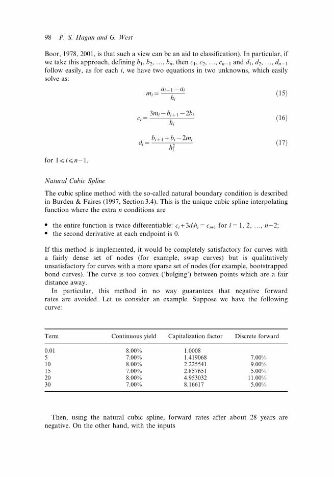
In particular, this method in no way guarantees that negative forward

rates are avoided. Let us consider an example. Suppose we have the following

curve:

Then, using the natural cubic spline, forward rates after about 28 years are

negative. On the other hand, with the inputs

Term Continuous yield Capitalization factor Discrete forward

0.01 8.00% 1.00085 7.00% 1.419068 7.00%10 8.00% 2.225541 9.00%15 7.00% 2.857651 5.00%20 8.00% 4.953032 11.00%30 7.00% 8.16617 5.00%


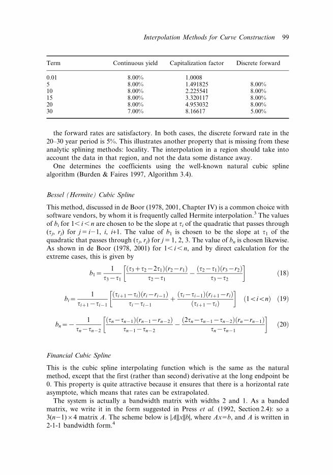
the forward rates are satisfactory. In both cases, the discrete forward rate in the

20–30 year period is 5%. This illustrates another property that is missing from these

analytic splining methods: locality. The interpolation in a region should take into

account the data in that region, and not the data some distance away.

One determines the coefficients using the well-known natural cubic spline

algorithm (Burden & Faires 1997, Algorithm 3.4).

Bessel (Hermite) Cubic Spline

This method, discussed in de Boor (1978, 2001, Chapter IV) is a common choice with

software vendors, by whom it is frequently called Hermite interpolation.3 The values

of bi for 1, i , n are chosen to be the slope at ti of the quadratic that passes through

(tj, rj) for j 5 i21, i, i+1. The value of b1 is chosen to be the slope at t1 of the

quadratic that passes through (tj, rj) for j 5 1, 2, 3. The value of bn is chosen likewise.

As shown in de Boor (1978, 2001) for 1, i , n, and by direct calculation for the

extreme cases, this is given by

b1~1

t3{t1

t3zt2{2t1ð Þ r2{r1ð Þt2{t1

{t2{t1ð Þ r3{r2ð Þ

t3{t2

� �ð18Þ

bi~1

tiz1{ti{1

tiz1{tið Þ ri{ri{1ð Þti{ti{1

zti{ti{1ð Þ riz1{rið Þ

tiz1{tið Þ

� �1vivnð Þ ð19Þ

bn~{1

tn{tn{2

tn{tn{1ð Þ rn{1{rn{2ð Þtn{1{tn{2

{2tn{tn{1{tn{2ð Þ rn{rn{1ð Þ

tn{tn{1

� �ð20Þ

Financial Cubic Spline

This is the cubic spline interpolating function which is the same as the natural

method, except that the first (rather than second) derivative at the long endpoint be

0. This property is quite attractive because it ensures that there is a horizontal rate

asymptote, which means that rates can be extrapolated.

The system is actually a bandwidth matrix with widths 2 and 1. As a banded

matrix, we write it in the form suggested in Press et al. (1992, Section 2.4): so a

3(n21)64 matrix A. The scheme below is |A||x||b|, where Ax5b, and A is written in

2-1-1 bandwidth form.4


0.01 8.00% 1.00085 8.00% 1.491825 8.00%10 8.00% 2.225541 8.00%15 8.00% 3.320117 8.00%20 8.00% 4.953032 8.00%30 7.00% 8.16617 5.00%


| |

| h1

2h1

3h1

h2

1 2h2

1 3h2

..

. ...

..

. ...

1 3hn{2

0 hn{1

1 2hn{1

��

��

0

h21

3h21

0

h22

3h22

0

..

.

..

.

0

h2n{1

3h2n{1

��

1

h31

{1

{1

h32

{1

{1

..

.

..

.

{1

h3n{1

|

b1

c1

d1

b2

c2

d2

b3

..

.

..

.

bn{1

cn{1

dn{1

��

��

0

a2{a1

0

0

a3{a2

0

0

..

.

..

.

0

an{an{1

0

��

The first equation above, c1 5 0, is the left-hand condition f 0(t1) 5 0. The last equation

above, bn{1z2cn{1hn{1z3dn{1h2n{1 ~ 0 is the right-hand condition f 9(tn) 5 0.

Cubic Spline on r(t)t

This is a cubic spline where the cubic spline is applied not to the function r(t) but to the

function r(t)t; it is this interpolating function that is required to be twice differentiable.

Thus, the nodes ti and values riti are passed into the cubic splining mechanism,

and the value r(t)t is returned. Thus, to find the value of r(t) for any given t, the

returned value needs to be divided by t:

r tð Þ~ aizbi t{tið Þzci t{tið Þ2zdi t{tið Þ3

ttiƒtƒtiz1 ð21Þ

Note that if f is the forward rate, then

f tð Þ~ LLt

r tð Þt

~biz2ci t{tið Þz3di t{tið Þ2 tiƒtƒtiz1

ð22Þ

We now consider two ways of solving for the coefficients.

Quadratic natural spline. The quadratic-natural splining method is proposed in

McCulloch & Kochin (2000). They argue that the usual natural cubic spline method

can have a ‘roller coaster’ output curve, particularly in the longer part of the curve

where there are fewer inputs. Essentially, the term is included as a weight in the

interpolation scheme, so for longer terms, the curve will certainly be stabilised. They

see as desirable properties that the curve be linear in the short end and asymptote in

the long end (so that extrapolation can be applied). These criteria are achieved by

making the endpoint constraints natural at the long end (i.e. the second derivative is0), but quadratic at the short end (i.e. the third derivative is 0). Making the second


derivative of r(t)t zero at the short end would make the first derivative of r(t) zero,

and this is contrary to typically observed features of yield curves.

The entire system of equations can once again be rewritten into a tridiagonal

system, in a way very much analogous to the ordinary cubic spline algorithm, and so

this is a special case implementation of Crout’s method of solving a tridiagonal system.

Bessel (Hermite) cubic spline. This method stands in relation to the Bessel method as

the quadratic-normal method stands in relationship to the natural cubic spline. Thus,

it is exactly the Bessel method, but applied to the function r(t)t rather than r(t).

Thus, the interpolation formulae are the same as (21) and (22).

Monotone Preserving Cubic Spline

This method is quite different from the others; it is a local method – the interpolatory

values are only determined by local behaviour, not global behaviour. Thus we are

not in the ‘linear algebra’ set-up of the previous methods, but have a different local

approach. Many of the ideas here will have a natural development later.

The method specifies the values of bi for 1(i(n. Note that c1, c2, …, cn21 and d1,

d2, …, dn21 follow directly from this, as seen in (16) and (17).

It is clear that a desirable criterion for interpolation of the yield curve is that the

geometry of the data points are preserved, i.e. there is no unexplained curvature, or

roller coaster, introduced. Such a method, based on the method of Fritsch & Butland

(1980), is developed in Hyman (1983). This method ensures that in regions of

monotonicity of the inputs (so, three successive increasing or decreasing values) the

interpolating function preserves this property. In the case of a local minimum or

maximum in the input discrete data, the output continuous interpolatory function

will preserve that property.

As before we have nodes t1, t2, …, tn and values r1, r2, …, rn. Define mesh sizes

and gradients

hi~tiz1{ti 1ƒiƒn{1ð Þ ð23Þ

mi~riz1{ri

hi

1ƒiƒn{1ð Þ ð24Þ

Now Hyman (1983) first defines

b1~2h1zh2ð Þm1{h1m2

h1zh2

bn~2hn{1zhn{2ð Þmn{1{hn{1mn{2

hn{1zhn{2

but simple examples show that this method may fail to be locally monotone

immediately to the interior side of the endpoints. In particular, negative forward

rates are possible, even likely. Thus, rather we define

b1~0~bn ð25Þ


We now define the gradients bi for 1, i , n. The curve is locally monotone at ti

(1 , i , n) if mi21mi > 0.

If the curve is not locally monotone, so it has a turning point, then we define bi50,

which ensures that the interpolant will also have a turning point there.

If the curve is locally monotone, we first define

bi~3mi{1mi

max mi{1, mið Þz2 min mi{1, mið Þ 1vivnð Þ ð26Þ

Then we also include the adjustment (Hyman 1983, Equation 2.3), which ensures

that no spurious extrema are introduced in the interpolated function. This

adjustment is

bi~min max 0, bið Þ, 3 min mi{1, mið Þð Þ if the curve is locally increasing at i

max min 0, bið Þ,3 max mi{1, mið Þð Þ if the curve is locally decreasing at i

�ð27Þ

Note that the requirement that the interpolatory curve preserves the geometry of

the curve does not guarantee that the forward function is positive.

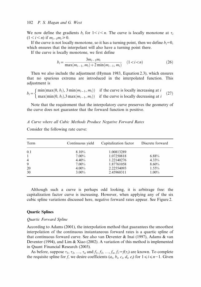
A Curve where all Cubic Methods Produce Negative Forward Rates

Consider the following rate curve:

Although such a curve is perhaps odd looking, it is arbitrage free: the

capitalization factor curve is increasing. However, when applying any of the six

cubic spline variations discussed here, negative forward rates appear. See Figure 2.

Quartic Splines

Quartic Forward Spline

According to Adams (2001), the interpolation method that guarantees the smoothest

interpolation of the continuous instantaneous forward rates is a quartic spline of

that continuous forward curve. See also van Deventer & Inai (1997), Adams & van

Deventer (1994), and Lim & Xiao (2002). A variation of this method is implemented

in Quant Financial Research (2003).

As before, suppose t1, t2, …, tn and f1, f2, …, fn, fi:5f(ti) are known. To complete

the requisite spline for f, we desire coefficients (ai, bi, ci, di, ei) for 1(i(n21. Given


0.1 8.10% 1.008132891 7.00% 1.07250818 6.88%4 4.40% 1.22140276 4.33%9 7.00% 1.87761058 8.60%20 4.00% 2.22554093 1.55%30 3.00% 2.45960311 1.00%


these coefficients, the function value at any term t will be

f tð Þ~aizbitzcit2zdit

3zeit4 tiƒtƒtiz1

5 ð28Þ

Hence

f 0 tð Þ~biz2citz3dit2z4eit

3

f 00 tð Þ~2ciz6ditz12eit2

f 000 tð Þ~6diz24eit

Requiring continuity of all of the above functions gives

fi~aizbitizcit2i zdit

3i zeit

4i 1ƒiƒn{1

fiz1~aizbitiz1zcit2iz1zdit

3iz1zeit

4iz1 1ƒiƒn{1

biz2citiz1z3dit2iz1z4eit

3iz1~biz1z2ciz1tiz1z3diz1t2

iz1z4eiz1t3iz1 1ƒiƒn{2

2ciz6ditiz1z12eit2iz1~2ciz1z6diz1tiz1z12eiz1t2

iz1 1ƒiƒn{2

6diz24eitiz1~6diz1z24eiz1tiz1 1ƒiƒn{2

Figure 2. The forward curves under various cubic interpolation methods for the given rates


Thus we have 5n-8 equations in 5n-5 unknowns. Thus, we need three more

conditions. The following three conditions are specified in Adams (2001):

N f 0(t1)50,

N f 9(tn)50,

N f 0(tn)50.

The system is actually a bandwidth matrix with widths 2 and 6. As a banded

matrix, we write it in the form suggested in Press et al. (1992, Section 2.4): so a

5(n21)69 matrix A. The scheme below is [A||x||b], where Ax5b, and A is written in

2-1-6 bandwidth form.

| |

| 1

1 tiz1

{1 {2tiz1

{2 {6tiz1

{6 {24tiz1

..

. ...

1 2tn

2 6tn

��

��

0

ti

t2iz1

{3t2iz1

{12t2iz1

0

..

.

3t2n

12t2n

��

0 2 6t1 12t21 0 0

t2i t3

i t4i 0 0 0

t3iz1 t4

iz1 0 0 0 0

{4t3iz1 0 1 2tiz1 3t2

iz1 4t3iz1

0 0 2 6tiz1 12t2iz1 0

0 0 6 24tiz1 0 0

..

. ... ..

. ... ..

. ...

4t3n | | | | |

| | | | | |

a1

bi

ci

di

ei

aiz1

..

.

dn{1

en{1

��

��

0

fi

fiz1

0

0

0

..

.

0

0

��

The first equation above is the first extra condition, while the last two equations

above are the other extra conditions.

This system is solved with the bandwidth matrix algorithms.

The bad news (and this should be expected) is that, like the cubic splining

methods, there is no guarantee of the absence of negative forward rates. These

methods are demanding such high smoothness criteria that any desired stiffness is

completely lost from the system. Thus, we can have enormous and completely

implausible fluctions in the output curve. For example, if we have the following

forward curve:

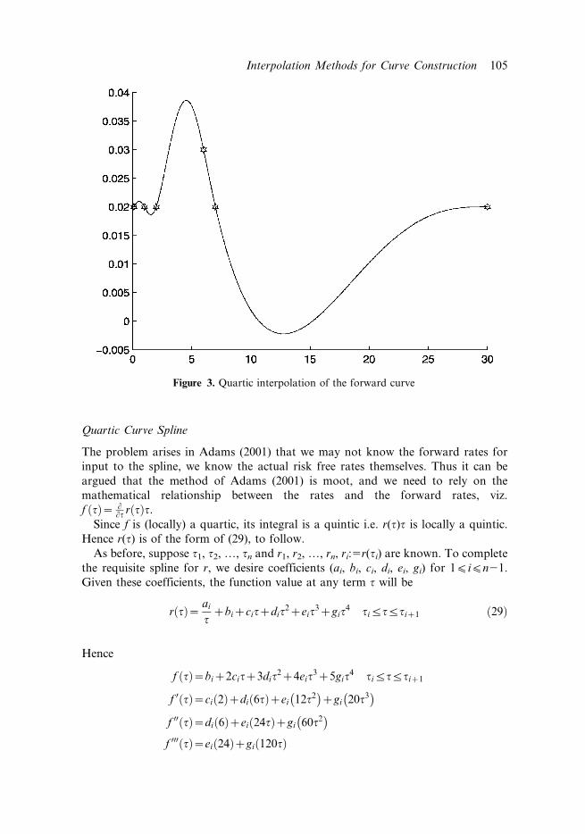
then the quartic spline on forwards has negative values. See Figure 3. By simply

adjusting the 6 year rate from 3% to 2%, we get a forward curve which is flat

everywhere, at 2%.

Term Instantaneous forward

0.1 2.00%1 2.00%2 2.00%6 3.00%7 2.00%30 2.00%


Quartic Curve Spline

The problem arises in Adams (2001) that we may not know the forward rates for

input to the spline, we know the actual risk free rates themselves. Thus it can be

argued that the method of Adams (2001) is moot, and we need to rely on the

mathematical relationship between the rates and the forward rates, viz.

f tð Þ~ LLt r tð Þt.

Since f is (locally) a quartic, its integral is a quintic i.e. r(t)t is locally a quintic.

Hence r(t) is of the form of (29), to follow.

As before, suppose t1, t2, …, tn and r1, r2, …, rn, ri:5r(ti) are known. To complete

the requisite spline for r, we desire coefficients (ai, bi, ci, di, ei, gi) for 1(i(n21.

Given these coefficients, the function value at any term t will be

r tð Þ~ ai

tzbizcitzdit

2zeit3zgit

4 tiƒtƒtiz1 ð29Þ

Hence

f tð Þ~biz2citz3dit2z4eit

3z5git4 tiƒtƒtiz1

f 0 tð Þ~ci 2ð Þzdi 6tð Þzei 12t2� �

zgi 20t3� �

f 00 tð Þ~di 6ð Þzei 24tð Þzgi 60t2� �

f 000 tð Þ~ei 24ð Þzgi 120tð Þ

Figure 3. Quartic interpolation of the forward curve


Requiring continuity of all of the above functions gives

ri~ai

ti

zbizcitizdit2i zeit

3i zgit

4i 1ƒiƒn{1

riz1~ai

tiz1zbizcitiz1zdit

2iz1zeit

3iz1zgit

4iz1 1ƒiƒn{1

biz2citiz1z3dit2iz1z4eit

3iz1z5git

4iz1

~biz1z2ciz1tiz1z3diz1t2iz1z4eiz1t3

iz1z5giz1t4iz1 1ƒiƒn{2

2ciz6ditiz1z12eit2iz1z20git

3iz1

~2ciz1z6diz1tiz1z12eiz1t2iz1z20giz1t3

iz1 1ƒiƒn{2

6diz24eitiz1z60git2iz1

~6diz1z24eiz1tiz1z60giz1t2iz1 1ƒiƒn{2

24eiz120gitiz1~24eiz1z120giz1tiz1 1ƒiƒn{2

Thus we have 6n210 equations in 6n26 unknowns. Thus, we need four more

conditions. It could be any four of the following, the first three of which are specified

in Adams (2001):6

N f 0(t1)50,

N f 9(tn)50,

N f 0(tn)50,

N f 90(tn)50.

N f 9(t1)50,

N r(t1)5f(t1), (as this must be the case as t1Q0),

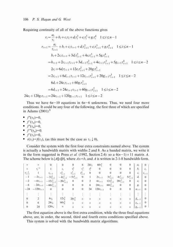
Consider the system with the first four extra constraints named above. The system

is actually a bandwidth matrix with widths 2 and 8. As a banded matrix, we write it

in the form suggested in Press et al. (1992, Section 2.4): so a 6(n21)611 matrix A.

The scheme below is |A||x||b|, where Ax5b, and A is written in 2-1-8 bandwidth form.

| |

| t{1i

t{1iz1 1

{1 {2tiz1

{2 {6tiz1

{6 {24tiz1

{24 {120tiz1

..

. ...

0 2

0 6

0 24

��

��

0

1

tiz1

{3t2iz1

{12t2iz1

{60t2iz1

0

..

.

6tn

24tn

120tn

0

ti

t2iz1

{4t3iz1

{20t3iz1

0

0

..

.

12t2n

60t2n

|

0 6 24t1 60t21 0 0 0

t2i t3

i t4i 0 0 0 0

t3iz1 t4

iz1 0 0 0 0 0

{5t4iz1 0 1 2tiz1 3t2

iz1 4t3iz1 5t4

iz1

0 0 2 6tiz1 12t2iz1 20t3

iz1 0

0 0 6 24tiz1 60t2iz1 0 0

0 0 24 120tiz1 0 0 0

..

. ... ..

. ... ..

. ... ..

.

20t3n | | | | | |

| | | | | | |

| | | | | | |

��

a1

bi

ci

di

ei

gi

aiz1

..

.

dn{1

en{1

gn{1

��

��

0

ri

riz1

0

0

0

0

..

.

0

0

0

��

The first equation above is the first extra condition, while the three final equations

above, are, in order, the second, third and fourth extra conditions specified above.

This system is solved with the bandwidth matrix algorithms.


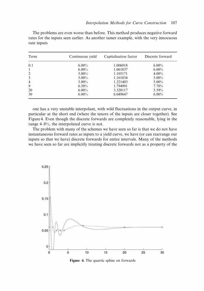
The problems are even worse than before. This method produces negative forward

rates for the inputs seen earlier. As another tamer example, with the very innocuous

rate inputs

one has a very unstable interpolant, with wild fluctuations in the output curve, in

particular at the short end (where the tenors of the inputs are closer together). See

Figure 4. Even though the discrete forwards are completely reasonable, lying in the

range 4–8%, the interpolated curve is not.

The problem with many of the schemes we have seen so far is that we do not have

instantaneous forward rates as inputs to a yield curve, we have (or can rearrange our

inputs so that we have) discrete forwards for entire intervals. Many of the methods

we have seen so far are implicitly treating discrete forwards not as a property of the

Term Continuous yield Capitalisation factor Discrete forward

0.1 6.00% 1.006018 6.00%1 6.00% 1.061837 6.00%2 5.00% 1.105171 4.00%3 5.00% 1.161834 5.00%4 5.00% 1.221403 5.00%9 6.50% 1.794991 7.70%20 6.00% 3.320117 5.59%30 6.00% 6.049647 6.00%

Figure 4. The quartic spline on forwards


entire interval, but as a property of the right endpoint of that interval, and ignore the

interval itself. We will change focus appropriately in the following section.

Forward Monotone Convex Spline

We introduce a new method: this spline is constructed to preserve appropriate

properties, principally among these the geometry of the inputs: the curve is locally

monotone and convex if the inputs show the analogous discrete properties.

Furthermore, if required, the curve is guaranteed to be positive if all the inputs

are positive. Because the method will explicitly include the possibility of a zero day

rate, we change notation slightly. Now we have terms 05t0, t1, …, tn and the generic

interval for consideration is [ti21, ti].

Construction of Suitable Discrete Forward Rates

Suppose the input at node i is f di . Rather than interpolate as if f d

i were the rate ‘only’

for time ti, we model f di as belonging to the entire interval [ti21, ti], and the rate at

the point ti as being

fi~ti{ti{1

tiz1{ti{1f diz1z

tiz1{ti

tiz1{ti{1f di , for i~1, 2, . . . , n{1 ð30Þ

f0~f d1 {

1

2f1{f d

1

� �, ð31Þ

fn~f dn {

1

2fn{1{f d

n

� �: ð32Þ

The interpolation algorithm will proceed on the rates fi. For i51, 2, …, n21 this

choice amounts to interpolating fi from the average values f diz1 and f d

i at the

midpoints of the adjacent intervals. The values f0 and fn were selected so that

f 9(0)505f 9(tn).

For some emerging markets, we may know the overnight rate f(0). If so, this

should be used for the end-point in preference to (31).

The Basic Interpolator

We require an interpolation function that satisfies the following properties:

f ti{1ð Þ~fi{1, f tið Þ~fi,1

ti{ti{1

Z ti

ti{1

f tð Þdt~f di ð33Þ

Let us postulate a quadratic of the form K + Lx(t) + Mx(t)2; one quickly gets from

(33) 3 linear equations in the unknowns K, L, M, which will solve as in (34):

f tð Þ~fi{1{ 4fi{1z2fi{6f di

� �x tð Þz 3fi{1z3fi{6f d

i

� �x tð Þ2 ð34Þ

~ 1{4x tð Þz3x tð Þ2�

fi{1z {2x tð Þz3x tð Þ2�

fiz 6x tð Þ{6x tð Þ2�

f di ð35Þ


where

x tð Þ~ t{ti{1

ti{ti{1ð36Þ

for i51, 2, …, n.

Here and later we use the following simple fact: suppose x : ~x sð Þ~ s{ti{1

ti{ti{1and

G95g. ThenZ t

ti{1

g x sð Þð Þ ds~ ti{ti{1ð Þ Gt{ti{1

ti{ti{1

�{G 0ð Þ

� �ð37Þ

Beyond tn, we should use flat extrapolation: f(t) 5 f(tn) for all t . tn.

In the next section we enforce monotonicity and convexity. Before doing this,

however, let us note some properties of the basic interpolator.

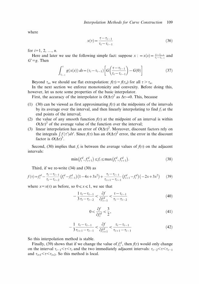
First, the accuracy of the interpolator is O(Dt)2 as DtR0. This, because

(1) (30) can be viewed as first approximating f(t) at the midpoints of the intervals

by its average over the interval, and then linearly interpolating to find fi at the

end points of the interval;

(2) the value of any smooth function f(t) at the midpoint of an interval is within

O(Dt)2 of the average value of the function over the interval;

(3) linear interpolation has an error of O(Dt)2. Moreover, discount factors rely on

the integralsR

f t0ð Þdt0. Since f(t) has an O(Dt)2 error, the error in the discount

factor is O(Dt)3.

Second, (30) implies that fi is between the average values of f(t) on the adjacent

intervals:

min f di , f d

iz1

� �ƒfiƒmax f d

i , f diz1

� �: ð38Þ

Third, if we re-write (34) and (30) as

f tð Þ~f di {

ti{ti{1

ti{ti{2f di {f d

i{1

� �1{4xz3x2� �

zti{ti{1

tiz1{ti{1f diz1{f d

i

� �{2xz3x2� �

ð39Þ

where x5x(t) as before, so 0(x(1, we see that

{1

3

ti{ti{1

ti{ti{2v

Lf

Lf di{1

v

t{ti{1

ti{ti{2ð40Þ

0v

Lf

Lf di

v

3

2, ð41Þ

{1

3

ti{ti{1

tiz1{ti{1v

Lf

Lf diz1

v

ti{ti{1

tiz1{ti{1ð42Þ

So this interpolation method is stable.

Finally, (39) shows that if we change the value of f di , then f(t) would only change

on the interval ti21,t,ti and the two immediately adjacent intervals: ti22,t,ti21

and ti+1,t,ti+2. So this method is local.


Enforcing Monotonicity and Convexity

We first analyse the monotonicity condition. Let us first focus on a single interval

ti21,t,ti. We require f(t) to be monotone increasing in this interval if and only if

f di{1vf d

i vf diz1

and to be monotone decreasing if and only if

f di{1 > f d

i > f diz1

Now, by considering (38), we see that a sufficient condition for our monotonicity

requirements over the ith interval are:

fi{1ƒf di ƒfi[f tð Þ is monotone increasing ð43Þ

fi{1§f di §fi[f tð Þ is monotone decreasing ð44Þ

Clearly monotonicity is not possible if fi{1vf di and f d

i > fi or fi{1 > f di and f d

i vfi.

Let us define

g tð Þ~f tð Þ{f di ð45Þ

for the interval [ti21, ti]. Denote gi215:g(ti21) gi:5g(ti), and note thatZ ti

ti{1

g tð Þdt~0 ð46Þ

and via (35) we have

g tð Þ~gi{1 1{4xz3x2� �

zgi {2xz3x2� �

ð47Þ

Now

Lg

Lx~gi{1 {4z6xð Þzgi {2z6xð Þ ð48Þ

In order to examine the extremum behaviour of g on [0, 1], we can simply analyse the

behaviour at 0 and at 1. Note that

g0 0ð Þ~{4gi{1{2gi

g0 1ð Þ~2gi{1z4gi

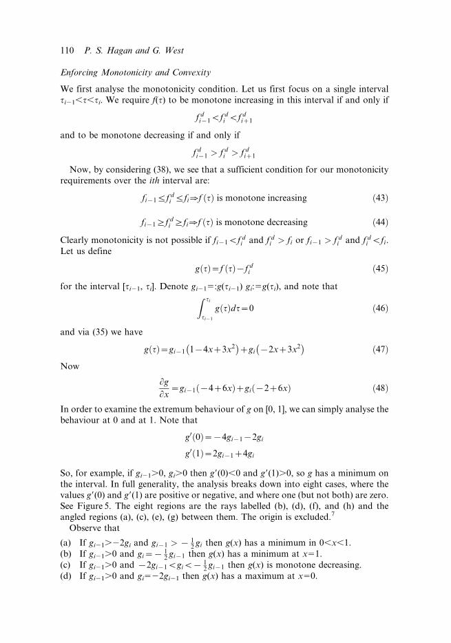
So, for example, if gi21.0, gi.0 then g9(0),0 and g9(1).0, so g has a minimum on

the interval. In full generality, the analysis breaks down into eight cases, where the

values g9(0) and g9(1) are positive or negative, and where one (but not both) are zero.

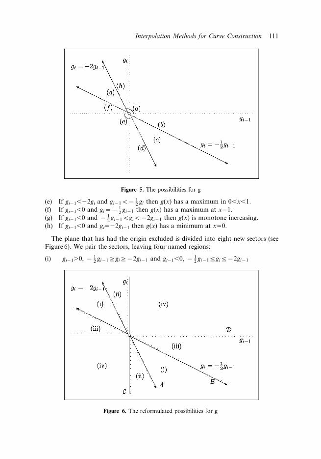
See Figure 5. The eight regions are the rays labelled (b), (d), (f), and (h) and the

angled regions (a), (c), (e), (g) between them. The origin is excluded.7

Observe that

(a) If gi21.22gi and gi{1 > { 12

gi then g(x) has a minimum in 0,x,1.

(b) If gi21.0 and gi~{ 12

gi{1 then g(x) has a minimum at x51.

(c) If gi21.0 and {2gi{1vgiv{ 12

gi{1 then g(x) is monotone decreasing.

(d) If gi21.0 and gi522gi21 then g(x) has a maximum at x50.


(e) If gi21,22gi and gi{1v{ 12

gi then g(x) has a maximum in 0,x,1.

(f) If gi21,0 and gi~{ 12

gi{1 then g(x) has a maximum at x51.

(g) If gi21,0 and { 12

gi{1vgiv{2gi{1 then g(x) is monotone increasing.

(h) If gi21,0 and gi522gi21 then g(x) has a minimum at x50.

The plane that has had the origin excluded is divided into eight new sectors (see

Figure 6). We pair the sectors, leaving four named regions:

(i) gi21.0, { 12

gi{1§gi§{2gi{1 and gi21,0, { 12

gi{1ƒgiƒ{2gi{1

Figure 5. The possibilities for g

Figure 6. The reformulated possibilities for g


(ii) gi21,0, gi.22gi21 and gi21.0, gi,22gi21

(iii) gi21.0, 0 > gi > { 12

gi{1 and gi21,0, 0vgiv{ 12

gi{1

(iv) gi21>0, gi>0 and gi21(0, gi(0

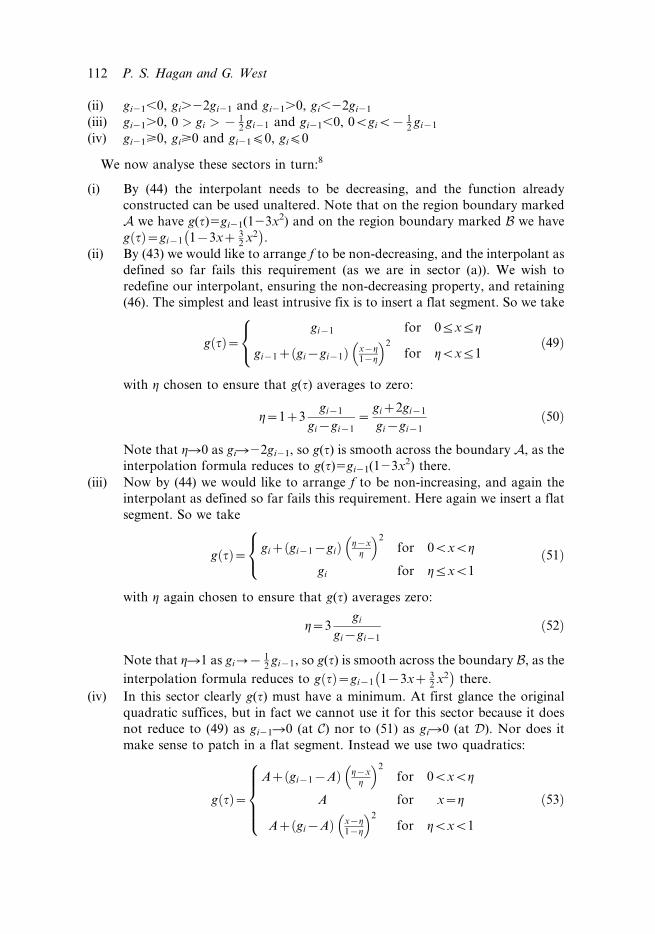
We now analyse these sectors in turn:8

(i) By (44) the interpolant needs to be decreasing, and the function already

constructed can be used unaltered. Note that on the region boundary marked

A we have g(t)5gi21(123x2) and on the region boundary marked B we have

g tð Þ~gi{1 1{3xz 32

x2� �

.

(ii) By (43) we would like to arrange f to be non-decreasing, and the interpolant as

defined so far fails this requirement (as we are in sector (a)). We wish to

redefine our interpolant, ensuring the non-decreasing property, and retaining

(46). The simplest and least intrusive fix is to insert a flat segment. So we take

g tð Þ~gi{1 for 0ƒxƒg

gi{1z gi{gi{1ð Þ x{g1{g

� 2

for gvxƒ1

8<

: ð49Þ

with g chosen to ensure that g(t) averages to zero:

g~1z3gi{1

gi{gi{1~

giz2gi{1

gi{gi{1ð50Þ

Note that gR0 as giR22gi21, so g(t) is smooth across the boundary A, as the

interpolation formula reduces to g(t)5gi21(123x2) there.

(iii) Now by (44) we would like to arrange f to be non-increasing, and again the

interpolant as defined so far fails this requirement. Here again we insert a flat

segment. So we take

g tð Þ~ giz gi{1{gið Þ g{xg

� 2

for 0vxvg

gi for gƒxv1

8<

: ð51Þ

with g again chosen to ensure that g(t) averages zero:

g~3gi

gi{gi{1ð52Þ

Note that gR1 as gi?{ 12

gi{1, so g(t) is smooth across the boundary B, as the

interpolation formula reduces to g tð Þ~gi{1 1{3xz 32

x2� �

there.

(iv) In this sector clearly g(t) must have a minimum. At first glance the original

quadratic suffices, but in fact we cannot use it for this sector because it does

not reduce to (49) as gi21R0 (at C) nor to (51) as giR0 (at D). Nor does it

make sense to patch in a flat segment. Instead we use two quadratics:

g tð Þ~Az gi{1{Að Þ g{x

g

� 2

for 0vxvg

A for x~g

Az gi{Að Þ x{g1{g

� 2

for gvxv1

8>>><

>>>:ð53Þ


where we need to set

A~{1

2ggi{1z 1{gð Þgi½ � ð54Þ

so that g(t) averages zero as required. We now need to pick g. To match the

preceding results, we need A50 at gi2150 and gi50. This means we need to

choose

g~1 if gi{1~0

0 if gi~0

�

We use the simplest choice

g~gi

gizgi{1ð55Þ

A~{gi{1gi

gi{1zgi

ð56Þ

Enforcing Positivity of the Interpolant

If the application requires it (as is the case for yield curves, for example) we may

guarantee that the instantaneous forward rates from the interpolation method are

always positive.

In the eight sectors, the maximum and minimum values of g(t) are:

gmin~gi{1, gmax~gi, for gi{1v0, gi > 0

gmin~{ gi{1gi

gi{1zgi, gmax~max gi{1, gif g, for gi{1 > 0, gi > 0

gmin~gi, gmax~gi{1, for gi{1 > 0, giv0

gmin~min gi{1, gif g, gmax~{ gi{1gi

gi{1zgi, for gi{1v0, giv0

ð57Þ

This is very promising. Whenever the data forces a maximum or minimum in the

interval, the maximum deviation from the average value is |gi21gi/(gi21+gi)|, which is

smaller than the smallest deviation of the endpoint.

For the applications of interest we may assume that all the average values f di , are

positive, for otherwise all interpolants f(t) would be zero somewhere. By (38) all the

fi are positive, except possibly f0 and fn.

Thus f(t) can only be negative if it has a negative local minimum within the

inteval, which occurs in the quadrant gi.0, gi21.0. Since gmin52gi21gi/(gi21+gi), it

suffices to require:

0vfi{1v3f di and 0vfiv3f d

i ð58Þ

To remain a reasonable distance away from 0, we require the more stringent:

0vfi{1v2f di and 0vfiv2f d

i ð59Þ


Thus, we apply where necessary the transformation9

f0?bound 0, f0, 2f d1

� �ð60Þ

fi?bound 0, fi, 2 min f di , f d

iz1

� �� i~1, 2, . . . , n{1 ð61Þ

fn?bound 0, fn, 2f dn

� �ð62Þ

If the application sets f0, then we cannot apply the first shift.

Amelioration of the Interpolant

By shifting the fi values we can make the interpolated curve smoother. The penalty is

that the interpolated function will be less local; in some intervals [ti21, ti] the value of

f(t) might depend on f dj for i22 ( j ( i + 2. Thus in any particular application we

must make a conscious decision as to whether we want the most locality or the best

smoothness.

Let us consider the value fi ; f(ti) between intervals i and i + 1. Suppose first that

f di > f d

i{1. If we also have f diz1 > f d

i , then f(t) is increasing in the interval i, and the

smoothest results occur when fi is in the range:

f di z

1

2f di {fi{1

� �vfivf d

i z2 f di {fi{1

� �ð63Þ

This is our target range, the range in which we would prefer fi to lie. Suppose now

that f diz1vf d

i . Then f(t) has a maximum in the interval. The maximum becomes

steadily smaller as fi increases towards f di , but our interpolation function becomes

increasingly asymmetric. In this case our target range is anything in

f di {

1

2l f d

i {fi{1

� �vfivf d

i ð64Þ

where the parameter 0(l(1 determines the smoothness of the interpolated

function. Experimentally l50.2 seems to work well.

We cannot afford to have criteria for fi which depend on values of f(t) at other

endpoints; this could lead to unpredictable non-locality and stability issues for

marginal gains in smoothness. Instead we use the linear approximation to fi21 as its

proxy. Thus, to get good smoothness results for the interval i, we would like fi to fall

in the range

f di z 1

2h{

i vf {i vf d

i z 12

h{i if f d

i{1vf di vf d

iz1

f di { 1

2lh{

i vf {i vf d

i if f di{1vf d

i , f di §f d

iz1

ð65Þ

The targets for fi if f di vf d

i{1 are obtained from similar considerations.

Thus, considerations about the smoothness within interval i leads to the target

range

f mini, 1 ƒfiƒf max

i, 1 ð66Þ


f mini, 1 ~min f d

i z 12

h{i , f d

iz1

� �,

f mini, 1 ~max f d

i { 12

lh{i , f d

iz1

� �,

f mini, 1 ~f d

i ,

f mini, 1 ~max f d

i z2h{i , f d

iz1

� �,

f maxi, 1 ~min f d

i z2h{i , f d

iz1

� �

f maxi, 1 ~f d

i

f maxi, 1 ~min f d

i { 12

lh{i , f d

iz1

� �

f maxi, 1 ~max f d

i z 12

h{i , f d

iz1

� �

if

if

if

if

f di{1vf d

i ƒf diz1

f di{1vf d

i , f di > f d

iz1

f di{1§f d

i , f di ƒf d

iz1

f di{1§f d

i > f diz1

ð67Þ

where

h{i ~

ti{ti{1

ti{ti{2f di {f d

i{1

� �ð68Þ

Similar considerations about the smoothness of f(t) in the interval i+1 lead to the

target ranges

f mini, 2 ƒfiƒf max

i, 2 ð69Þ

f mini, 2 ~max f d

iz1{2hzi , f d

i

� �,

f mini, 2 ~max f d

iz1z12

lhzi , f d

i

� �,

f mini, 2 ~f d

iz1,

f mini, 2 ~min f d

iz1{12

hzi , f d

i

� �,

f maxi, 2 ~max f d

iz1{12

hzi , f d

i

� �if f d

i vf diz1ƒf d

iz2

f maxi, 2 ~f d

iz1 if f di vf d

iz1, f diz1 > f d

iz2

f maxi, 2 ~min f d

iz1z12

lhzi , f d

i

� �if f d

i §f diz1, f d

iz1vf diz2

f maxi, 2 ~min f d

iz1{2hzi , f d

i

� �if f d

i §f diz1§f d

iz2

ð70Þ

where

hzi ~

tiz1{ti

tiz2{ti

f diz2{f d

iz1

� �ð71Þ

To ameliorate the max’s, min’s, and general ugliness of the interpolant, we use the

following procedure:

(a) add an additional interval at the beginning and the end:

t{1~t0{ t1{t0ð Þ, f d0 ~f d

1 {t1{t0

t2{t0f d2 {f d

1

� �ð72Þ

tnz1~tnz tn{tn{1ð Þ, f dnz1~f d

n ztn{tn{1

tn{tn{2f dn {f d

n{1

� �ð73Þ

(b) Select the fi’s by linearly interpolating on the midpoints of the intervals:

fi~ti{ti{1

tiz1{ti{1f diz1z

tiz1{ti

tiz1{ti{1f di , for i~0, 1, . . . , n ð74Þ

Note that with the false intervals, this formula works for i50 and i5n.

(c) For each i51, 2, …, n21,

(i) if the target ranges overlap, define the common range

max f mini, 1 , f min

i, 2

� ƒfiƒmin f max

i, 1 , f maxi, 2

� ð75Þ

If fi is outside this common range, make the minimum adjustment to fi to


place it in the common range:

if fivmax f mini, 1 , f min

i, 2

� set fi~max f min

i, 1 , f mini, 2

�

if fi > min f maxi, 1 ,f max

i, 2

� set fi~min f max

i, 1 , f maxi, 2

� ð76Þ

(ii) if the target ranges don’t overlap, define the gap by

min f maxi, 1 , f max

i, 2

� ƒfiƒmax f min

i, 1 , f mini, 2

� ð77Þ

If fi is below or above the gap, make the minimum adjustment to fi to place

it on the edge of the gap:

if fivmin f maxi, 1 , f max

i, 2

� set fi~min f max

i, 1 , f maxi, 2

�

if fi > max f mini, 1 , f min

i, 2

� set fi~max f min

i, 1 , f mini, 2

� ð78Þ

(d) if now f0{f d0

�� > 12

f1{f d0

�� , replace f0 with

f0~f d1 {

1

2f1{f d

0

� �ð79Þ

provided we don’t know the value of f0 (some markets explicitly quote f0.)

(e) Similarly, if fn{f dn

�� > 12

fn{1{f dn

�� , replace fn with

fn~f dn z

1

2f dn {fn{1

� �ð80Þ

(f) If the application requires f(t).0 apply the transformations in (60), (61) and

(62).

Stripping the BMA Basis Factor

As an example, consider stripping the Bond Market Association Municipal Swap

Index basis factor. The BMA index is an index of tax-exempt Variable Rate Demand

Notes issued by Municipalities. In a BMA basis swap, the BMA rate would be paid

quarterly against a percentage of 3 month LIBOR for a specified number of years. In

order to get the forward BMA one thus needs to bootstrap the LIBOR curve, fit this

‘percentage’ curve, and multiply. To fit this percentage curve is one of the toughest

stripping problems around. Consider the input data for 9 May 2003, percentages for

swaps of differing expiry dates, as follows:

15-May-03 0.884562607-Aug-03 0.884562606-Nov-03 0.921857926-May-04 0.9433488212-May-05 0.86603225


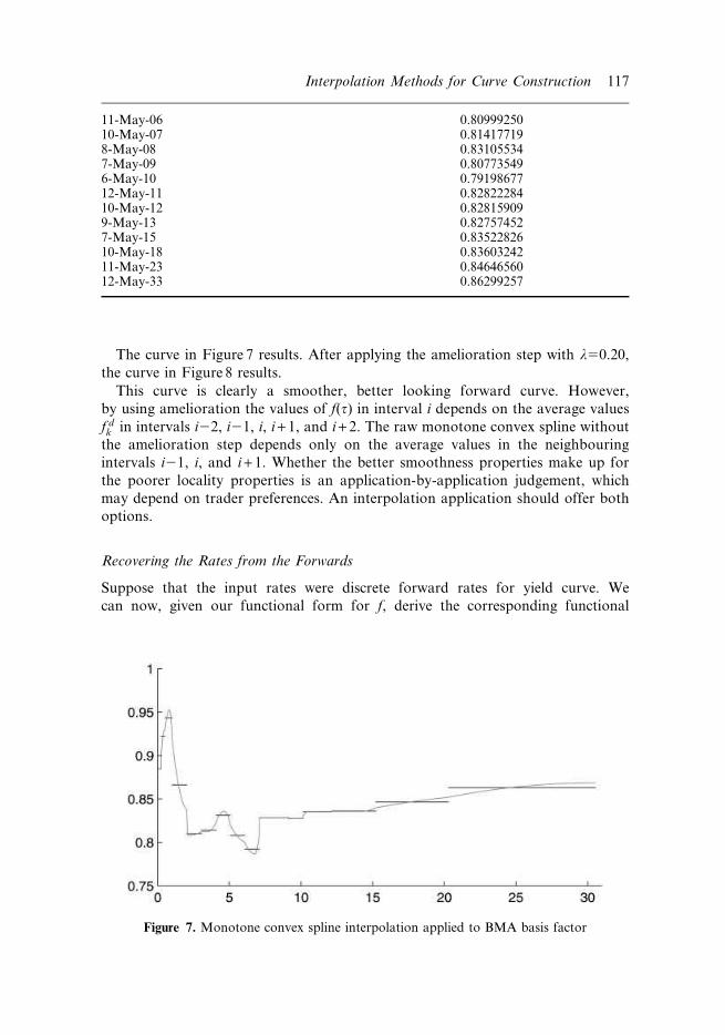
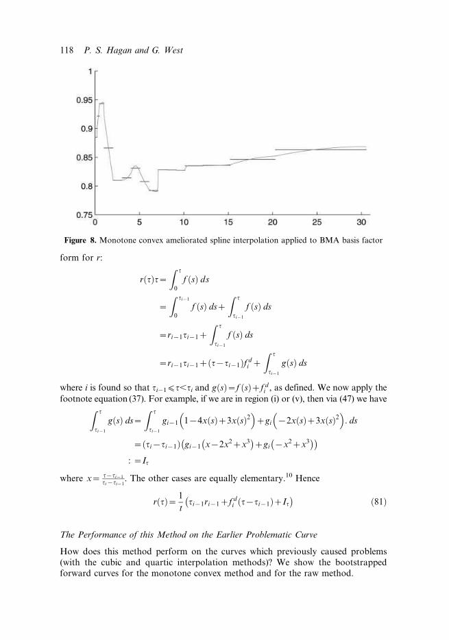
The curve in Figure 7 results. After applying the amelioration step with l50.20,

the curve in Figure 8 results.

This curve is clearly a smoother, better looking forward curve. However,

by using amelioration the values of f(t) in interval i depends on the average values

f dk in intervals i22, i21, i, i + 1, and i + 2. The raw monotone convex spline without

the amelioration step depends only on the average values in the neighbouring

intervals i21, i, and i + 1. Whether the better smoothness properties make up for

the poorer locality properties is an application-by-application judgement, which

may depend on trader preferences. An interpolation application should offer both

options.

Recovering the Rates from the Forwards

Suppose that the input rates were discrete forward rates for yield curve. We

can now, given our functional form for f, derive the corresponding functional

11-May-06 0.8099925010-May-07 0.814177198-May-08 0.831055347-May-09 0.807735496-May-10 0.7919867712-May-11 0.8282228410-May-12 0.828159099-May-13 0.827574527-May-15 0.8352282610-May-18 0.8360324211-May-23 0.8464656012-May-33 0.86299257

Figure 7. Monotone convex spline interpolation applied to BMA basis factor


form for r:

r tð Þt~Z t

0

f sð Þ ds

~

Z ti{1

0

f sð Þ dsz

Z t

ti{1

f sð Þ ds

~ri{1ti{1z

Z t

ti{1

f sð Þ ds

~ri{1ti{1z t{ti{1ð Þf di z

Z t

ti{1

g sð Þ ds

where i is found so that ti21(t,ti and g sð Þ~f sð Þzf di , as defined. We now apply the

footnote equation (37). For example, if we are in region (i) or (v), then via (47) we haveZ t

ti{1

g sð Þ ds~

Z t

ti{1

gi{1 1{4x sð Þz3x sð Þ2�

zgi {2x sð Þz3x sð Þ2�

: ds

~ ti{ti{1ð Þ gi{1 x{2x2zx3� �

zgi {x2zx3� ��

: ~It

where x~ t{ti{1

ti{ti{1. The other cases are equally elementary.10 Hence

r tð Þ~ 1

tti{1ri{1zf d

i t{ti{1ð ÞzIt

� �ð81Þ

The Performance of this Method on the Earlier Problematic Curve

How does this method perform on the curves which previously caused problems

(with the cubic and quartic interpolation methods)? We show the bootstrappedforward curves for the monotone convex method and for the raw method.

Figure 8. Monotone convex ameliorated spline interpolation applied to BMA basis factor


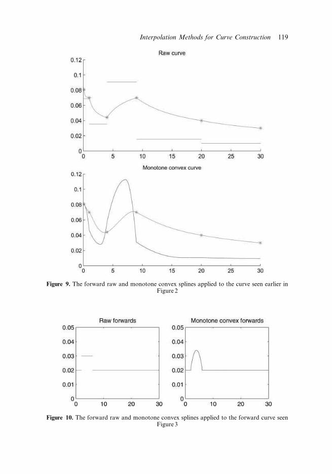
Figure 9. The forward raw and monotone convex splines applied to the curve seen earlier inFigure 2

Figure 10. The forward raw and monotone convex splines applied to the forward curve seenFigure 3


A Minimalist Quadratic Interpolator

The Minimalist Interpolator

We introduce another new interpolation method. We seek an interpolator of the

(forward) rates of the form

f tð Þ~aizbi t{ti{1ð Þzci t{ti{1ð Þ2 ti{1ƒtƒti ð82Þ

for 1(i(n. The first requirement will be that

1

ti{ti{1

Z ti

ti{1

f tð Þdt~f di ð83Þ

Let hi5ti2ti21 much as before. By elementary calculus, we find that this

requirement is

f di ~aiz

1

2bihiz

1

3cih

2i i~1, 2, . . . , n ð84Þ

This condition alone guarantees that the inputs to the curve are recovered by the

interpolation scheme. The second requirement will be that the interpolant is

continuous: clearly this simply means

aiz1~aizbihizcih2i i~1, 2, . . . , n{1 ð85Þ

The Penalty Function

Thus we have 2n21 linear equations in 3n unknowns. The coefficients are

finalised not by imposing a further n+1 linear constraints, as we have seen

previously, but rather by minimizing an error function. Typical further linear

constraints would be making the first or second derivatives continuous. Rather

we will attempt to minimize a penalty function composed of sum of squares of

the jumps in the first derivatives across the boundaries and sum of squares of the

second derivatives, with a relative (user input) weighting between the two

penalties.

Note that

f 0 tð Þ~biz2ci t{ti{1ð Þ ð86Þ

f 00 tð Þ~2ci ð87Þ

Let us now define the jumps in the first derivatives, and the weighted values in the

second derivative, for attempted minimization:

J1, i~biz1{bi{2cihi i~1, 2, . . . , n{1 ð88Þ

J2, i~2cihi i~1, 2, . . . , n ð89Þ


The penalty function, which we hope to minimize, is defined, for some prescribed

w g (0,1), as

Pw~wXn{1

i~1

J21, iz 1{wð Þ

Xn

i~1

J22, i ð90Þ

So we have a minimization problem subject to the constraints (84), (85), which

suggests a Lagrange multiplier approach to the problem. We have 2n21 constraints

in 3n variables, so n+1 degrees of freedom: thus, the setting is well formulated. So, for

notational purposes, we define a 3n vector x5(a1, b1, c1, a2, …, an, bn, cn); under this

notational realignment we have

0~x3i{2z1

2x3i{1hiz

1

3x3ih

2i {f d

i : ~gi xð Þ i~1, 2, . . . , n ð91Þ

0~x3i{2zx3i{1hizx3ih2i {x3iz1 : ~gnzi xð Þ i~1, 2, . . . , n{1 ð92Þ

Pw~wXn{1

i~1

x3iz2{x3i{1{2x3ihið Þ2z4 1{wð ÞXn

i~1

x23ih

2i

Now introducing Lagrange multipliers l1, l2, …, l2n21 we have the solution

+Pw~X2n{1

k~1

lk+gk

in other words

LPw

Lxi

~X2n{1

k~1

lk

Lgk

Lxi

i~1, 2, . . . , 3n ð93Þ

Let z5(x1, x2, …, x3n, l1, l2, …, l2n21) be the unknown and required vector. We

have a system of 5n21 equations ((91), (92) and (93)) in the same number of

unknowns z1, z2, …, z5n21:

0~ F½ �i

~

{z3nz1{z4nz1 if i~1

{z3nz iz2ð Þ=3zz4n{1z iz2ð Þ=3{z4nz iz2ð Þ=3 if i~4, 7, . . . , 3n{5

{z4nzz5n{1 if i~3n{2

{2w z5{z2{2z3h1ð Þ{z3nz112

h1{z4nz1h1 if i~2

2w {zi{3{2zi{2h i{2ð Þ=3z2ziz2ziz1h iz1ð Þ=3{ziz3

� �

{z3nz iz1ð Þ=312

h iz1ð Þ=3{z4nz iz1ð Þ=3h2iz1ð Þ=3 if i~5, 8, . . . , 3n{4

2w z3n{1{z3n{4{2z3n{3hn{1ð Þ{z4n12

hn if i~3n{1

{4w ziz2{zi{1{2zihi=3

� �z8 1{wð Þzih

2i=3{z3nzi=3

13

h2i=3{z4nzi=3h2

i=3 if i~3, 6, . . . , 3n{3

8 1{wð Þz3nh2n{z4n

13

h2n if i~3n

z3 i{3nð Þ{2z12

z3 i{3nð Þ{1hi{3nz13

z3 i{3nð Þh2i{3n{f d

i{3n if 3nz1ƒiƒ4n

z3 i{4nð Þ{2zz3 i{4nð Þ{1hi{4nzz3 i{4nð Þh2i{4n{z3 i{4nð Þz1 if 4nz1ƒiƒ5n{1

8>>>>>>>>>>>>>>>>>>>>>>>>>>>><

>>>>>>>>>>>>>>>>>>>>>>>>>>>>:


This can be written as a linear system Az5v where

vi~f di{3n if 3nz1ƒiƒ4n

0 otherwise

(

This we solve with straightforward Gaussian elimination and back substitution, as

seen in the algorithm in Press et al. (1992, Section 2.3).

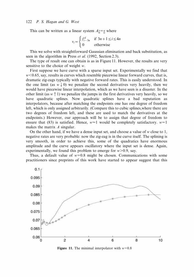
The type of result one can obtain is as in Figure 11. However, the results are very

sensitive to the choice of weight w.

First suppose we have curve with a sparse input set. Experimentally we find that

w,0.65, say, results in curves which resemble piecewise linear forward curves, that is,

dramatic zig-zags typically with negative forward rates. This is easily understood. Inthe one limit (as wQ0) we penalize the second derivatives very heavily, then we

would have piecewise linear interpolation, which as we have seen is a disaster. In the

other limit (as wq1) we penalize the jumps in the first derivatives very heavily, so we

have quadratic splines. Now quadratic splines have a bad reputation as

interpolators, because after matching the endpoints one has one degree of freedom

left, which is only assigned arbitrarily. (Compare this to cubic splines,where there are

two degrees of freedom left, and these are used to match the derivatives at the

endpoints.) However, our approach will be to assign that degree of freedom toensure that (83) is satisfied. Hence, w<1 would be completely satisfactory. w51

makes the matrix A singular.

On the other hand, if we have a dense input set, and choose a value of w close to 1,

negative rates are very probable: now the zig-zag is in the curve itself. The splining is

very smooth, in order to achieve this, some of the quadratics have enormous

amplitude and the curve appears oscillatory where the input set is dense. Again,

experimentally, we found this problem to emerge for w.0.9, say.

Thus, a default value of w50.8 might be chosen. Communications with some

practitioners since preprints of this work have started to appear suggest that this

Figure 11. The minimal interpolator with w50.8


method is very popular. However, this method does not guarantee positive forward

rates, nor is it local. In fact, empirically its behaviour is often similar to the

behaviour we have seen for some of the cubic or quartic spline algorithms.

Nevertheless, this approach deserves attention, because it correctly interprets the

information provided as information about intervals, not as information about the

endpoint of the interval. Additional conditions to guarantee that each forward is

positive on the domain of interest would need to be introduced, and penalty

minimization under these conditions appears to be non-trivial.

Construction Quality Criteria

Our focus so far has mainly been on analysing if the curves generated ‘look good’

and if the forwards are positive and continuous. As promised earlier, we now

consider the other three construction quality criteria we have isolated.

Localness of an Interpolation Method

Suppose we move the input at ti. We wish to determine the interval (ti2l, ti+u) on

which the yield curve values change. Clearly it is desirable that l and u be as small as

possible. The results for yield curve interpolation are reported in Figure 12. For

forward curve interpolation they are shown in Figure 13.

Some interesting observations arise. Among cubic and quartic splining methods,

one of the Bessel methods or the monotone piecewise cubic method are the most

attractive. The splines that use clamping at either end are all unatractive insofar as

Figure 12. The localness indices for curve interpolation methods


this criterion is concerned. As expected, the simple methods described earlier are the

most local. Finally, using amelioration in the monotone convex method

compromises locality only very slightly.

Forward Stability

We want to measure how stable an interpolation method is – given a change in one

of the inputs, how much can the output interpolated curve be changed? We measure

this noise feature on the yield curve rates or on the forwards – both as inputs and as

outputs. Appropriate norms for any interpolation method a given yield curve, or a

given forward curve, would be

M rð Þk k~ supt

maxi

Lr tð ÞLri

��

��

M fð Þk k~ supt

maxi

Lf tð ÞLf d

i

��

��

where the input rates are r1, r2, …, rn or f d1 , f d

2 , . . . , f dn respectively, and the

bootstrapped curves are r and f respectively.

Except in some simple cases, these norms cannot be determined analytically, and

would need to be estimated empirically. In those cases for any given curve this was

achieved by measuring the maximum difference, in the supremum norm, between the

original bootstrapped curve, and any of the 2n curves which arise when any of the n

nodes are blipped up or down by one basis point. The difference was estimated by

testing at discrete points along the entire curve, in steps of 0.01 of a year. These two

measures (the theoretical derivative measure and the discrete measure) will be

equivalent up to the scaling constant 10000 (since mathematically one basis point is

1000021), so in actual fact we will take the value found empirically and multiply it by

10000.

The second issue is to decide over what set of curves to calculate this norm. For

this we simply considered a fairly large set of plausible curves that we have seen

trading in various markets.

Clearly all of the earlier methods then have a norm of 1. The later arguments show

that the monotone convex method initially has a norm of 1.5, although this will be

compromised by the modifications which enforce monotonicity and convexity, and

then by the amelioration of the interpolant. We found that, with an extensive set of

Figure 13. The localness indices for forward interpolation methods


plausible test curves, the norm for this method, unameliorated and with amelioration

at l50.2, was never more than about 2.

All other methods, with the exception of the two quartic methods, had norms

varying from about 1.2 to about 1.6. Perhaps the fact that the monotone convex

method has a slightly worse norm is to be expected: more constraints are being

imposed, so the norm should be higher. The two quartic methods had norms inexcess of 100000 for our test set, and we have no reason to expect that, in the class of

arbitrage free curves, these methods have finite norm. The instability observed was

gross, and seemed to be the rule more than the exception.

Localness of Hedges

What we assume is that exactly the instruments which were used to bootstrap the

yield curve are those that are available for creating hedge portfolios. Given aportfolio with certain risky cashflows, we wish to construct the portfolio of these

underlying instruments that will hedge those cash flows.

We assume that the set of risky cash flows are all known, for example, swaps have

been decomposed into a fixed coupon bond and a floating rate note, the latter of

which has been discarded as riskless, and any flows with optionality have had some

sort of Greek substitution as flows without optionality. Finally, we assume that we

are in the world where our bootstrap prices all of the inputs exactly.

In order to proceed with this analysis, we first review the two classic approaches tohedging: bumping and waves.

In bumping, we form new curves indexed by j: to create the jth curve one bumps

up the jth input rate by say 1 basis point, bootstraps the curve again, and reprices the

risky portfolio with the new curve; the difference between the new and old price

forms a vector DV, indexed by the bootstrapping instruments.

One now calculates the matrix P where Pij is the change in price of the jth

bootstrapping instrument under the ith curve. As each of the bootstraps prices the

input set exactly to par, this matrix is diagonal: it is only the original instrument,which reprices now that that fair rate has changed. The hedge vector Q is chosen to

satisfy PQ5DV.

The portfolio Q perfectly hedges the given risky portfolio exactly under the case

where the valuation curve moves from exactly one of the inputs being blipped by

1bp. One then hopes that the portfolio provides an adequate hedge against more

general moves. Typically 1 bp is small enough to be in the linear regime, and so one

is adequately protected against all small changes in the inputs.

In waves: one approach is to again form new curves, again indexed by i: the ith

curve has the original yield curve incremented by a triangle, with left hand endpoint

at ti21, height of say 1 or 10 basis points and apex at ti, and right hand endpoint at

ti+1. (The first and last triangle will in fact be right angled, with their apex at the first

and last time points respectively.) The matrix P is defined as before. This time we see

that P is not diagonal, but is typically upper triangular – if there are no overlapping

inputs then the ith curve is the same as the mark to market curve before time ti21, so

if i.j, then the jth instrument does not change in value under this curve. (An example

where we have no overlapping inputs would be where we have LIBOR instrumentsto 3 months, then 366, 669, 9612, 12615, 15618 FRAs, and then annual swaps.


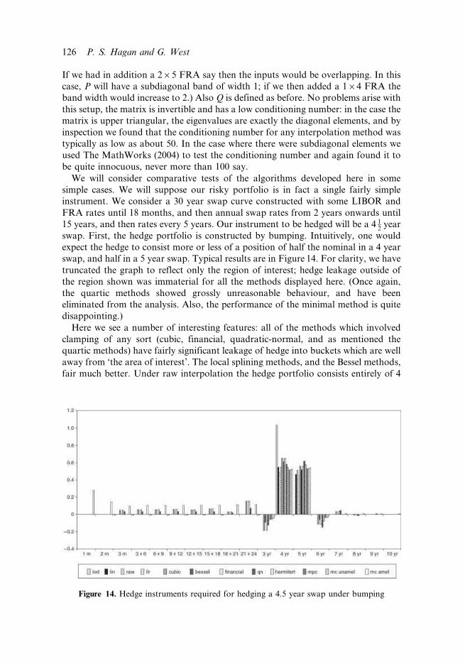
If we had in addition a 265 FRA say then the inputs would be overlapping. In this

case, P will have a subdiagonal band of width 1; if we then added a 164 FRA the

band width would increase to 2.) Also Q is defined as before. No problems arise with

this setup, the matrix is invertible and has a low conditioning number: in the case the

matrix is upper triangular, the eigenvalues are exactly the diagonal elements, and by

inspection we found that the conditioning number for any interpolation method was

typically as low as about 50. In the case where there were subdiagonal elements we

used The MathWorks (2004) to test the conditioning number and again found it to

be quite innocuous, never more than 100 say.

We will consider comparative tests of the algorithms developed here in some

simple cases. We will suppose our risky portfolio is in fact a single fairly simple

instrument. We consider a 30 year swap curve constructed with some LIBOR and

FRA rates until 18 months, and then annual swap rates from 2 years onwards until

15 years, and then rates every 5 years. Our instrument to be hedged will be a 4 12

year

swap. First, the hedge portfolio is constructed by bumping. Intuitively, one would

expect the hedge to consist more or less of a position of half the nominal in a 4 year

swap, and half in a 5 year swap. Typical results are in Figure 14. For clarity, we have

truncated the graph to reflect only the region of interest; hedge leakage outside of

the region shown was immaterial for all the methods displayed here. (Once again,

the quartic methods showed grossly unreasonable behaviour, and have been

eliminated from the analysis. Also, the performance of the minimal method is quite

disappointing.)

Here we see a number of interesting features: all of the methods which involved

clamping of any sort (cubic, financial, quadratic-normal, and as mentioned the

quartic methods) have fairly significant leakage of hedge into buckets which are well

away from ‘the area of interest’. The local splining methods, and the Bessel methods,

fair much better. Under raw interpolation the hedge portfolio consists entirely of 4

Figure 14. Hedge instruments required for hedging a 4.5 year swap under bumping


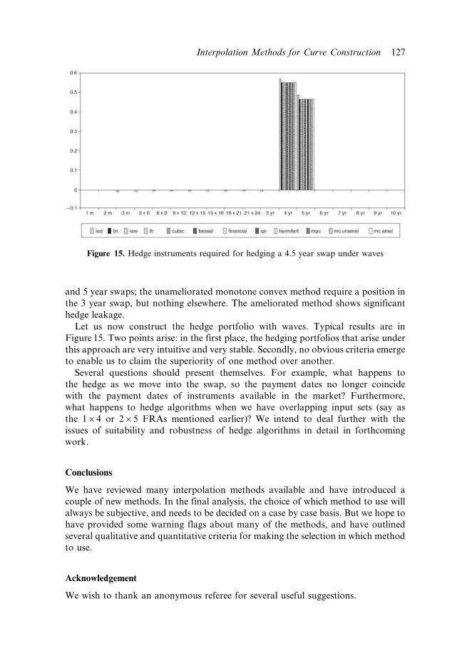
and 5 year swaps; the unameliorated monotone convex method require a position in

the 3 year swap, but nothing elsewhere. The ameliorated method shows significant

hedge leakage.

Let us now construct the hedge portfolio with waves. Typical results are in

Figure 15. Two points arise: in the first place, the hedging portfolios that arise under

this approach are very intuitive and very stable. Secondly, no obvious criteria emerge

to enable us to claim the superiority of one method over another.

Several questions should present themselves. For example, what happens to

the hedge as we move into the swap, so the payment dates no longer coincide

with the payment dates of instruments available in the market? Furthermore,

what happens to hedge algorithms when we have overlapping input sets (say as

the 164 or 265 FRAs mentioned earlier)? We intend to deal further with the

issues of suitability and robustness of hedge algorithms in detail in forthcoming

work.

Conclusions

We have reviewed many interpolation methods available and have introduced a

couple of new methods. In the final analysis, the choice of which method to use will

always be subjective, and needs to be decided on a case by case basis. But we hope to

have provided some warning flags about many of the methods, and have outlined

several qualitative and quantitative criteria for making the selection in which method

to use.

Acknowledgement

We wish to thank an anonymous referee for several useful suggestions.

Figure 15. Hedge instruments required for hedging a 4.5 year swap under waves


Notes

1 By this we mean the intervals between the fixed payments of the swap, such as three or six months.2 For example, it is not reasonable to expect a bootstrapper to differentiate bonds according to tax status,

rather, some value adjustment should be made a priori to the prices one set of bonds or the other, so that

what is input can be considered to have the same tax status.3 To paraphrase the nomenclature of de Boor (1978, 2001): a cubic spline where the first derivative is

known (in addition to the function values) is called a Hermite spline. The Bessel method is an

intermediate method, where the derivatives are estimated from the function values, and then the Hermite

method is applied.4 A matrix in a-1-b bandwidth form means that the entry in the ith row and jth column in this

representation actually lies in the ith row and i + j2a21th column in the canonical matrix representation.

Note that the entries in the top left and bottom right of the bandwidth matrix are redundant, they can be

set to anything. This redundancy is denoted by a 6.5 Why not f(r)5ai + bi(r2ri) + ci(r2ri)

2 + di(r2ri)3 + ei(r2ri)

4? We would prefer on principle this format.

However, the bandwidth matrices which result are very unwieldy.6 This observation is consistent with Adams (2001) where, after interpolating the forward curves, one

additional piece of information is needed to recover the interpolatory function on the yields i.e. the

method of Adams (2001) has one remaining degree of freedom.7 If gi21505gi, then the curve is flat, and g50.8 It is advisable to ensure no problems with code execution (‘division by zero’) to trap the cases x(r)50 and

x(r)51 up front: in these cases, g(r)5gi21 and g(r)5gi respectively.9 The bound function is given by bound(a, x, b)5min(max(a, x), b).10 The same trapping as before has Iti{1

~0~Iti.

References

Adams, K. (2001) Smooth interpolation of zero curves, Algo Research Quarterly, 4(1/2), pp. 11–22.

Adams, K. J. and van Deventer, D. R. (1994) Fitting yield curves and forward rate curves with maximum

smoothness, Journal of Fixed Income, June 4(1), pp. 52–62.

Burden, R. L. and Faires, J. D. (1997) Numerical Analysis, 6th edn (Brooks Cole).

Cox, J. C. et al. (1985) A theory of the term structure of interest rates, Econometrica, 53, pp. 385–407.

de Boor, C. (1978, 2001) A Practical Guide to Splines: Revised Edition, Vol. 27 of Applied Mathematical

Sciences (New York: Springer-Verlag).

Fritsch, F. and Butland, J. (1980) An improved monotone piecewise cubic interpolation algorithm,

Lawrence Livermore National Laboratory Preprint UCRL.

Heath, D. et al. (1990) Bond pricing and the term structure of interest rates: a discrete time approximation,

Journal of Financial and Quantitative Analysis, 25, pp. 419–440.

Hull, J. (2002) Options, Futures, and Other Derivatives, 5th edn (Prentice Hall).

Hull, J. and White, A. (1990) Pricing interest rate derivative securities, Review of Financial Studies, 3.

Hyman, J. M. (1983) Accurate monotonicity preserving cubic interpolation, SIAM Journal on Scientific

and Statistical Computing, 4(4), pp. 645–654.

Lim, K. and Xiao, Q. (2002) Computing maximum smoothness forward rate curves, Statistics and

Computing, 12, pp. 275–279.

Lin, B.-H. (2002) Fitting term structure of interest rates using B-Splines: the case of Taiwanese

government bonds, Applied Financial Economics, 12(1), pp. 57–75.

McCulloch, J. H. and Kochin, L. A. (2000) The inflation premium implicit in the US real and nominal

term structures of interest rates, Technical Report 12, Ohio State University Economics Department.

*http://www.econ.ohio-state.edu/jhm/jhm.html

Press, W. H. et al. (1992) Numerical Recipes in C: the Art of Scientific Computing, 2nd edn (Cambridge

University Press).

Quant Financial Research (2003) The BEASSA zero coupon yield curves: technical specifications,

Technical report, Bond Exchange of South Africa. *http://www.bondex.co.za/pricing/

BEASSA_Zero_Curves_Tech_Specs_240504.pdf


Ron, U. (2000) A practical guide to swap curve construction. Technical Report 17, Bank of Canada.

*http://www.bankofcanada.ca/en/res/wp00-17.htm

The MathWorks (2004) Matlab Version 7, The MathWorks, Inc.

van Deventer, D. R. and Inai, K. (1997) Financial Risk Analytics - A Term Structure Model Approach for

Banking (Irwin: Insurance and Investment Managemen).

Vasicek, O. A. (1977) An equilibrium characterisation of the term structure, Journal of Financial

Economics, 15.

Zangari, P. (1997) An investigation into term structure estimation methods for RiskMetrics, RiskMetrics

Monitor, Third Quarter, pp. 3–48.


Interpolation Methods for Curve Construction · Interpolation Methods for Curve Construction...

Documents

Transcript of Interpolation Methods for Curve Construction · Interpolation Methods for Curve Construction...