Internship Report

Natural convection flows inside differentially heated cavities

written by

Pim Adriaan Bullee, BSc.University of Twente

conducted at

POLOResearch Laboratories for Emerging Technologies in Cooling and Thermophysics

UFSCThe Federal University of Santa Catarina

in the period

March - June 2014

under supervision of

Prof H.W.M. HoeijmakersUniversity of Twente

Prof C.J. DeschampsFederal University of Santa Catarina

1

Abstract

A natural convection driven flow inside a differentially heated square cavity with aspectratio 4 is studied. The cavity is filled with water and the Rayleigh number is determinedto be 1.14×1010. Measurement results from different heights obtained using Laser DopplerVelocimetry are presented. These results were used together with a literature study tomake a statement regarding the results obtained by another researcher using the samecavity. Concluded is that because of a mistake made when setting up the measurementequipment, his results regarding the flow field near the cold wall are invalid. Apart fromthis, special care is taken in optimizing the measurement procedure by reviewing thenumber of measurements required to obtain a reliable average velocity value. Thereby thenumber of seeding particles inside the cavity that visualize the flow is optimized.

i

Nomenclature and abbreviations

Cp specific heat capacity [kJ/(kg K)]fdoppler frequency related to the light scattered by the particles [1/s]fshift change in frequency due to Bragg cell [1/s]fsignal frequency of the signal captured by the receiving optics [1/s]g acceleration due to gravity [m/s2]h convective heat transfer coefficient [W/(m2 K)]H height of the cavity 0.4 [m]k thermal conductivity [W/(m K)]n refractive indexp static pressure [N/ms2]rw radius of laser beam waist [m]t thickness of the acrylic wallT temperature [K]~u velocity vector of the flow [m/s]vn velocity normal to the lines of the interference pattern [m/s]

Dimensionless numbersNuH Nusselt number based on the cavity height; see Eq. 1.8Pr Prandtl number fluid property; see Eq. 1.7RaH Rayleigh number based on the cavity height; see Eq. 1.6

Greek symbolsα thermal diffusivity α = k/ρCp [m2/s]β volume expansion coefficient [1/K]∆T temperature difference between the heated walls [K]θ angle of incident or transmitted lightµ dynamic viscosity [kg/(m s)]ν kinematic viscosity [m2/s]ρ density [kg/m3]¯τ viscous stress tensor [kg/ms2]

Subscriptsa airc cold wallg acrylic glassh hot walls surfacew water∞ sufficiently far away (underscore ∞)

ii

AbbreviationsAR aspect ratio height versus widthCFD computational fluid dynamicsDNS direct numerical simulationLDV Laser Doppler velocimetryLHS left hand side of the equationODE ordinary differential equationPDE partial differential equationRHS right hand side of the equation

iii

Contents

1 Theoretical introduction 11.1 Introduction to heat transfer . . . . . . . . . . . . . . . . . . . . . . . . . . 11.2 Mechanisms of natural convection . . . . . . . . . . . . . . . . . . . . . . . . 31.3 Natural convection in a rectangular closed cavity . . . . . . . . . . . . . . . 41.4 Dimensionless numbers . . . . . . . . . . . . . . . . . . . . . . . . . . . . . . 5

2 Theoretical background 82.1 Governing equations . . . . . . . . . . . . . . . . . . . . . . . . . . . . . . . 82.2 Exact solution . . . . . . . . . . . . . . . . . . . . . . . . . . . . . . . . . . 92.3 Literature review . . . . . . . . . . . . . . . . . . . . . . . . . . . . . . . . . 122.4 Laser Doppler velocimetry . . . . . . . . . . . . . . . . . . . . . . . . . . . 18

3 The experiment 213.1 Experimental setup . . . . . . . . . . . . . . . . . . . . . . . . . . . . . . . . 213.2 Experimental procedure and settings . . . . . . . . . . . . . . . . . . . . . . 253.3 Measurement of confined fluids . . . . . . . . . . . . . . . . . . . . . . . . . 26

4 Results 284.1 Number of particles in the cavity . . . . . . . . . . . . . . . . . . . . . . . . 294.2 Number of data readings . . . . . . . . . . . . . . . . . . . . . . . . . . . . . 304.3 Velocity profiles . . . . . . . . . . . . . . . . . . . . . . . . . . . . . . . . . . 30

5 Conclusions and discussion 335.1 Number of particles in the cavity . . . . . . . . . . . . . . . . . . . . . . . . 335.2 Number of data readings . . . . . . . . . . . . . . . . . . . . . . . . . . . . . 345.3 Velocity profiles . . . . . . . . . . . . . . . . . . . . . . . . . . . . . . . . . . 345.4 Recommendations for further research . . . . . . . . . . . . . . . . . . . . . 365.5 Recommendations for the lab . . . . . . . . . . . . . . . . . . . . . . . . . . 37

A Measurement results by Popinhak 42

iv

Preface

This report is written during my three month internship in Florianopolis, Brazil. The goalof the research was to measure the flow field inside a rectangular cavity. This flow fieldis the result of natural convection inside the cavity, caused by a temperature differencebetween the two side walls. Together with me worked three bachelor students; Heitor,Domicio and Marcelo. They were of great help with my work and by the time I left, theywere able to continue the measurements on their own.

The cavity we used had already been build and used before. However, it required mainte-nance. Rust was removed and some parts were painted again. The setup used to measurethe temperature inside the cavity was redesigned and rebuild to be more durable. Themeasurement equipment had not been used since a long time as well. Therefore a lotof knowledge on the operation and maintenance of it had gone lost. Even the operatingmanuals and some parts of the setup were missing. Since no-one working at POLO hadany experience in operating the measurement equipment, I spent my first two months alot of time on finding out how to operate the equipment. Also a lot of time went intomaintenance, testing, setting up to equipment and acquiring all the lost documents andparts. At some point even an external technician had to be of assistance. His conclusionwas that the measurement equipment was in a state far from optimal. Nonetheless, in thelast month I managed to perform some measurements and was able to finish my work.

To be of assistance to future researchers working in the lab, I decided in the first periodof my internship to write an extensive operations manual. It is titled ’LDV MeasurementManual’ and co-authored by Heitor Paes de Andrade. Since it features to much specificinformation and instructions, I decided against adding it to this report. It is handed intogether with this report, but should be regarded as a separate piece of work, since itserves the sole intention of being of assistance to others working in the LDV lab at POLO.

This whole process made that I obtained a lot of knowledge on the measurement setup andequipment, which ultimately helped me in reaching the final conclusions of this report.It also resulted in that I had a lot of information and a lot of time to write it all down.The result is a substantial report and equally sized measurement manual. To compensatethe reader who is more familiar with the subject, I wrote an extensive two page summary,which covers the most important parts of this report.

v

Extensive summary

The subject of study in this report is a natural convection driven flow inside a rectangularcavity. The cavity has dimensions 10 x 10 x 40 cm (width x depth x height) and is filledwith water. The two side walls of the cavity are subjected to a temperature differenceof ten degree Celsius. Near the hot wall, the water moves upwards due to the buoyancyeffect. Near the cold wall the water moves downwards for the same reasons. The Rayleighnumber for this setup is calculated to be 1.14×1010 using Equation 1.6. Based on theliterature study presented in Section 2.3, it is concluded that for this Rayleigh number theflow inside the cavity is in the turbulent regime.

The natural convection driven flow inside a cavity models many practical engineering ap-plications [1]. Thereby it also functions as a benchmark problem to validate numericalmodels [2]. Between 2010 and 2013, Andre Popinhak build and worked with the samesetup as described in this report [3]. His results are shown in Figure A.1. The flow profilesnear the cold wall are a bit different from the results obtained by other researchers. Forinstance Trias et al. performed numerical simulations at a Rayleigh number of 1.0×1010.As can be seen in Figure 2.3, their results display symmetry between the hot and the coldwall side of the cavity in terms of the averaged velocity and temperature fields [2]. Theresults obtained by Popinhak do not show this symmetry. In his results, the flow profilesnear the cold wall show a mere sinusoidal shape. This behaviour is explained by Popinhakas being caused by the fluid changing direction after encounter with the bottom wall. Thisresults in a fluid intrusion moving upwards which disturbs the flow [3]. This particularphenomena is not present in the work by Trias et al.. Relevant experimental research hasbeen conducted by Saury et al.. They worked with Rayleigh numbers between 4.0×1010

and 1.2×1011 [4]. Although their results do not display the perfect symmetry as was foundnumerically by Trias et al., a clear distinction exists with the results reported by Popin-hak. The sinusoidal flow behaviour near the cold wall side of the cavity is not reportedby Saury et al., nor is there mention given of an upwards travelling intrusion [4]. Sincethe near hot wall side results of Popinhak do show resemblance to the results obtainedby both Trias et al. and Saury et al., there is reason enough to check the results fromPopinhak by redoing his measurements.

The flow velocities in the cavity are measured using Laser Doppler Velocimetry (LDV)equipment. Polyamid particles with a diameter of 0.5 µm are added to the water in the

vi

cavity to enhance the visibility of the flow. It turned out to be very important to addthe correct amount of particles, since otherwise the measurement equipment was unableto detect the flow. In the operations manual of the measurement equipment is given thatthe optimal particle density is equal to the inverse of the measurement volume created bythe LDV equipment [5]. The optimal total amount of particles to be added to the cavitywas calculated to be ranging between 6×10−3 and 7×10−3 gram.

To create a flow profile, the flow velocity is measured at multiple points in the cavity. Todetermine the velocity at a specific point, the average velocity is calculated from multipleparticles passing that point. To increase the efficiency of the measurements, the numberof particles needed for an accurate average velocity is revised. In Figure 4.1 is shown thatafter 100 measurements, the average velocity is well within the boundaries of rounding.The data used to create one of the flow profiles is also shown to convergence in Figure 4.2.

The flow profiles at different heights in the cavity are plotted in Figure 4.3. The resultsnear the hot wall side at half cavity height are missing due to time limitations. The flowprofiles near the cold wall side of the cavity show, in contrary to the hot wall side, noresemblance to the results produced by Popinhak. The flow profiles near both the hot andthe cold wall do show resemblance to the results from Trias et al. and Saury et al. as citedin [2] and [4].

The results presented in this report are produced identical to the way Popinhak producedhis results. In order to gain further insight in what causes the difference in results, thesettings files used by Popinhak to set up the measurement equipment are examined. Thesefiles were found on the computer used to perform measurements in the lab. Two of thevariables that have to be set are related to the filter applied to the signal captured by themeasurement equipment. Evaluation of the values chosen by Popinhak showed that thebandwidth of the filter that was chosen by Popinhak is to small. With his filter settings,only velocities ranging between -2.6 and 7.5 mm/s were allowed to pass. As can be seenin Figure 4.3, the velocities inside the cavity range between -8.5 and 8.5 mm/s. ThereforePopinhak was unable to correctly measure the velocities near the cold wall side.

What can not be explained is why a velocity of 8.5 mm/s shows up in the results fromPopinhak in Figure A.1e and a velocity of -3 mm/s in Figure A.1i. Also, the cold wallresults appear to be sinusoidal instead of a cut-off normal velocity profile. Since Popinhakgives in his master’s thesis no information on the filter settings used, the reliability of hisresults is questionable.

It is therefore concluded, based on the wrongly chosen filter, the results presented inFigure 4.3 and the work of two different authors working with comparable setups, thatthe results and conclusions presented by Popinhak regarding the near cold wall velocitiesobtained using LDV measurements can be regarded as incorrect.

vii

Chapter 1

Theoretical introduction

1.1 Introduction to heat transfer

All natural phenomena strive to reach an equilibrium or, a lowest state of energy. This canfor instance be seen in a ball, which will always fall to the ground in order to minimize itsgravitational energy. Or think of the water in a very quiet lake which is always levelled.There are never peaks and after a disturbance, the surface of the water will be flat again.The same goes for heat; nature always tries to redistribute heat to reach a constantequilibrium temperature. Placing a hot cup of coffee inside a room is metaphoricallythe same as throwing a little stone inside the quiet like. The disturbance, the local risein temperature, will eventually be evened out and the cup of coffee will have the sametemperature as its surroundings.

Conduction Conduction is the transport of heat on a molecular level. Particles witha higher energy transfer their energy in the form of heat to neighbouring particles withless energy. In gasses and liquids, this interaction is in the form of collisions and diffusiondue to random motion of the particles. In solids, conduction is due to the vibrations ofthe atoms and the energy transport by free electrons. The amount of heat that can betransported by conduction is dependent of the material properties of the medium, butalso on its dimensions and the temperature difference[6]. The amount of conductive heattransfer is defined using Equation 1.1

Qcond = −kA∆T

∆x(1.1)

In this equation k denotes the thermal conductivity [W/(m K)], which is a measure forthe ability of a material to conduct heat. A denotes the area of the material normal tothe direction of the conductive heat transfer, whereas ∆x denotes the thickness of thematerial. By taking the limit of ∆x→ 0 the equation is reduced to Fourier’s law of heatconduction, which is given in Equation 1.2. It is named after Jean Baptiste Joseph Fourier,who first came up with this expression in 1822 [6].

Qcond = −kAdTdx

(1.2)

1

Radiation The best example of heat transfer by means of radiation is the energy fromthe sun that reaches the earth. This is by far the fastest way of energy transportation,since it travels at the speed of light. The energy transportation takes place in the form ofelectromagnetic waves which do not require the presence of any sort of medium; radiationfrom the sun travels through space which is a vacuum. Thermal radiation is emitted byobjects due to their temperature and is therefore different from other types of radiationsuch as x-ray and microwaves. Thermal radiation can be felt by humans while x-ray andmicrowaves are senseless. Thermal radiation can for instance be observed when walkingpast a stone wall after a hot day. The wall has been heated by the sun all day andstill maintains and radiates this heat during the cooler evening. The amount of heattransported by radiation is defined using the Stefan-Boltzmann law in Equation 1.3. Itresulted from and was named after the combined works of Ludwig Boltzmann and JozefStefan by the end of the 19th century.

Qemit = σωAsT4s (1.3)

The σ in Equation 1.3 denotes the Stefan-Boltzmann constant, equal to 5.67 ×10−8

[W/(m2 K4)]. Different types of materials display different emissivity behaviour. There-fore ε gives the material dependent emissivity varying between 0 and 1. Aluminium foilfor instance has a very low emissivity with an ε value of 0.07, whilst black and white painthave values of 0.98 and 0.90 respectively. A theoretically perfect radiating so called ‘blackbody’ has an ε value of 1 [6]. The surface area and its temperature are denoted by As andTs respectively.

Convection Apart from energy transfer due to the random motion of molecules (con-duction), the motion of the fluid will also transport heat in the presence of a temperaturedifference. The motion of the fluid is determined by the stream velocity of the flow. Sothe faster the fluid flows, the larger is the amount of heat transfer by convection. Anexample of this is blowing over a hot cup of soup. When blowing harder the soup will cooldown faster and by not blowing at all the soup will cool down more slowly. The process ofconvection is actually conduction with fluid motion [6]. Consider for instance a hot solidblock of material, being cooled by an airflow. The first very thin layer of air which is indirect contact with the block will have no velocity. This is called the no-slip boundarycondition. It is caused by the viscosity of the fluid causing the fluid to stick to the wallof the block. Due to this zero velocity, heat can only be transferred from the block to theadjacent layer of air by the mechanism of conduction. In layers of air further away fromthe block this energy is carried away by convection. The rate of convective heat transfer islinear with the temperature difference and can be expressed using Newton’s law of coolinggiven in Equation 1.4.

Qconv = hAs(Ts − T∞) (1.4)

In this equation h is the convective heat transfer coefficient [W/(m2 K)]. It is not a fluidproperty, but depends on all variables influencing the convection. Of influence are forinstance the surface geometry, the nature of fluid motion and its properties as well as

2

the fluid velocity. Therefore the convective heat transfer coefficient is to be determinedexperimentally [6]. The temperature sufficiently far away from the surface is denoted bythe subscript ∞. Convection can be driven by for instance using a fan, called forced con-vection, but the type of convection observed in this research is natural convection. Thismeans that the fluid motion is not influenced by an external source but is caused by therising of warmer particles creating a flow.

It is important to understand that usually heat transfer is due to a combination of themechanisms of convection, conduction and radiation. One of the mechanisms can bedominant over the others, which mostly depends on environmental conditions.

1.2 Mechanisms of natural convection

A local change in temperature of a fluid will almost always result in an instability, or atleast a distributed temperature field inside the fluid. For instance when a fluid at rest isheated from below and cooled from above, a situation is created where the cooler, moredense fluid lies on top of the warmer less dense fluid. This is an unstable situation and at acertain moment the warmer and less dense fluid will move upwards to float on the cooler,more dense fluid. The cooler layer will move downwards where it is heated, to expand andmove upwards again. This results in a circulating vertical flow due to the constant heatingand cooling and associated expansion and contraction of the fluid. The driving force forthis phenomena is buoyancy, the same principle on which the floatation of ships and hotair balloons is based. A body of a certain density submerged in a medium with a higherdensity will experience, due to buoyancy, a force directed upwards. The size of the forceis related to the amount of volume of the body that is actually submerged, which is thesame as the amount of fluid displaced. This is known as Archimedes’ principle (Eureka!),and is displayed in mathematical form in Equation 1.5.

Fbuoyancy = ρfluid gVdisplaced (1.5)

In this equation g is the acceleration due to gravity (9.8 m/s2), ρ is the density [kg/m3]and V is the volume [m3] of the fluid displaced.

When a natural convection flow will start to develop is, apart from the temperaturedifference, also depended of the fluid viscosity and the thermal conduction rate. For fluidswith a high thermal conduction coefficient, the differences in temperature, and thus thedensity, will be more evenly distributed. So, for these types of fluids, heat transportationdue to conduction is dominant over heat transport due to convection. Viscous forcesinside the fluid and where the fluid is in contact with another medium (for instance a wallover which the fluid flows) counteract the movement of the fluid. So, for fluids with highviscosity coefficients, the temperature differences (and thus the differences in density) needto be larger in order to start a buoyancy driven flow. This threshold was first expressedby Rayleigh in the early 20th century and will be discussed in more detail in Section 1.4.

3

1.3 Natural convection in a rectangular closed cavity

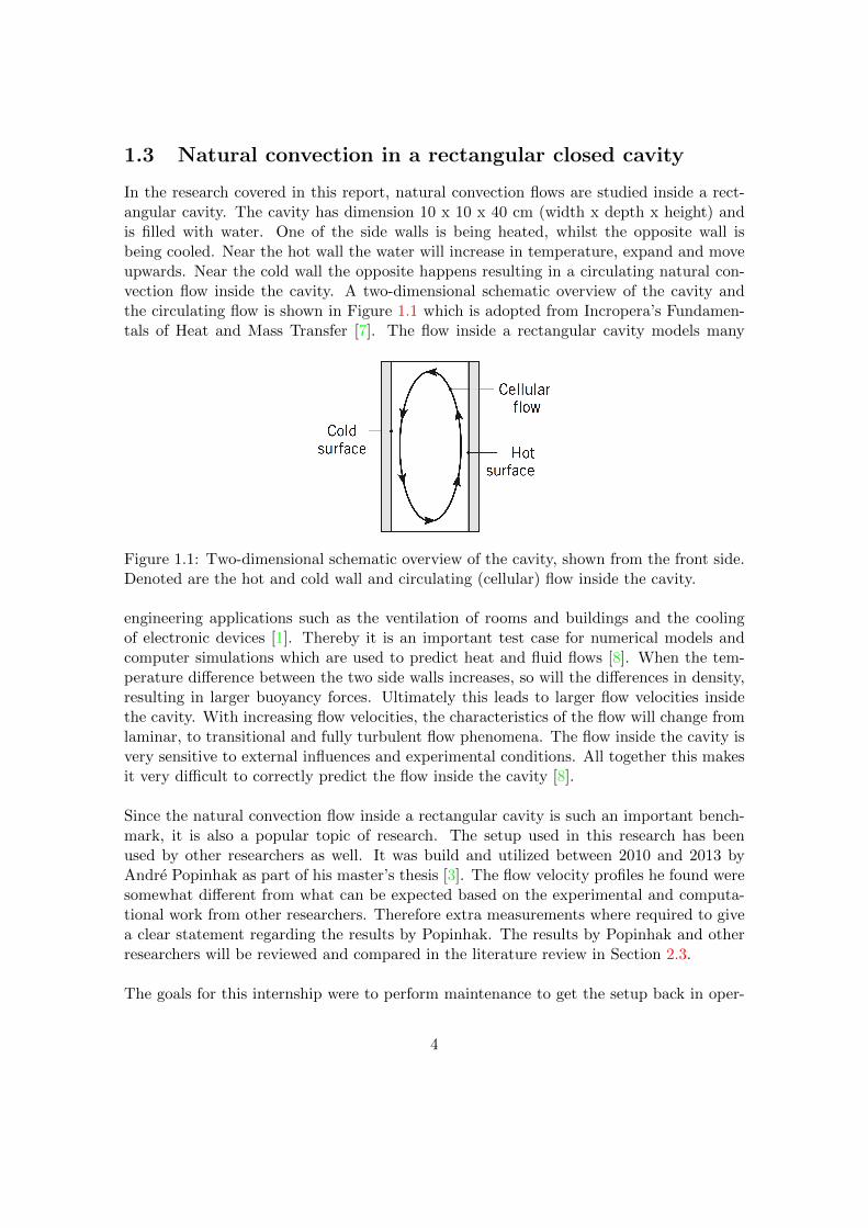
In the research covered in this report, natural convection flows are studied inside a rect-angular cavity. The cavity has dimension 10 x 10 x 40 cm (width x depth x height) andis filled with water. One of the side walls is being heated, whilst the opposite wall isbeing cooled. Near the hot wall the water will increase in temperature, expand and moveupwards. Near the cold wall the opposite happens resulting in a circulating natural con-vection flow inside the cavity. A two-dimensional schematic overview of the cavity andthe circulating flow is shown in Figure 1.1 which is adopted from Incropera’s Fundamen-tals of Heat and Mass Transfer [7]. The flow inside a rectangular cavity models many

Figure 1.1: Two-dimensional schematic overview of the cavity, shown from the front side.Denoted are the hot and cold wall and circulating (cellular) flow inside the cavity.

engineering applications such as the ventilation of rooms and buildings and the coolingof electronic devices [1]. Thereby it is an important test case for numerical models andcomputer simulations which are used to predict heat and fluid flows [8]. When the tem-perature difference between the two side walls increases, so will the differences in density,resulting in larger buoyancy forces. Ultimately this leads to larger flow velocities insidethe cavity. With increasing flow velocities, the characteristics of the flow will change fromlaminar, to transitional and fully turbulent flow phenomena. The flow inside the cavity isvery sensitive to external influences and experimental conditions. All together this makesit very difficult to correctly predict the flow inside the cavity [8].

Since the natural convection flow inside a rectangular cavity is such an important bench-mark, it is also a popular topic of research. The setup used in this research has beenused by other researchers as well. It was build and utilized between 2010 and 2013 byAndre Popinhak as part of his master’s thesis [3]. The flow velocity profiles he found weresomewhat different from what can be expected based on the experimental and computa-tional work from other researchers. Therefore extra measurements where required to givea clear statement regarding the results by Popinhak. The results by Popinhak and otherresearchers will be reviewed and compared in the literature review in Section 2.3.

The goals for this internship were to perform maintenance to get the setup back in oper-

4

ational condition, to redo the measurements performed by Popinhak and try to find anexplanation for his somewhat anomalous results.

1.4 Dimensionless numbers

Dimensionless numbers are very useful to undo certain phenomena or problems from un-necessary context. For most applications, the quantity of a certain measure is not ofimportance, rather the ratio with respect to another measure is what matters. This canfor instance be seen in scale models of aircraft wings in wind tunnels. By defining the po-sition on the wing relative to the total width (chord length) of the wing, the experimentalresults for a small wing can be translated to a larger wing of the same shape.In this research dimensionless numbers are used to compare results from different re-searchers who use different test setups in terms of dimensions, temperatures and types offluid.

Rayleigh number Buoyancy driven flows were first studied by Benard in 1900 [9]. Heworked with very thin layers of fluid (a millimetre or less) that where heated from belowand in contact with open air from above. In the fluid he discovered convection cells thatwhere created when natural convection occurred. Each cell occupied a small volume insidethe fluid where locally the fluid rises on one side of the cell and descends on the other sideof the cell. Together this forms the so called cellular flow. Inspired by Benard, Rayleighstarted working on the theoretical background of this phenomena and came in 1916 with aratio between the buoyancy on the one hand, and the viscosity and thermal conduction ofthe fluid on the other hand. He showed that when the ratio exceeds a certain threshold, aconvective flow starts to develop. For values well below this value, heat transfer is mainlyin the form of conduction [10]. This ratio found by Rayleigh is nowadays known as theRayleigh number. It is defined in Equation 1.6 by making use of Equation 11.21 fromKundu’s Fluid Mechanics as cited in [10].

RaL =gβ∆TL3

να(1.6)

In this research, the temperature difference ∆T is defined as the difference between thetwo heated walls ∆T = Th−Tc. The temperatures Th and Tc are chosen 28 and 18 degreeCelsius with a working (environmental) temperature Tw of 23 degree Celsius. The typicallength scale L of the setup is chosen to be the height of the cavity H, which is equal to 0.4metre. The kinematic viscosity ν of the water inside the cavity at the specified workingtemperature is found using extrapolation and has a value of 9.4030 ×10−7 [m2/s] [11]. Thethermal diffusivity α of the water is given by α = k/ρCp [m2/s]. The value for the thermalconductivity k of the water was taken to be equal to 0.58 [W/(m K)] at a temperature of 25deg Celsius [11]. The extrapolated values for the density ρ and the specific heat capacityCp of the water inside the cavity at the specified working temperature were found to beequal to 997.44 [kg/m3] and 4.1803 [kJ/(kg K)] respectively [11]. Filling in these numbersresults in a Rayleigh number of 1.14×1010.

5

Prandtl number The German physicist Ludwin Prandtl (1875 - 1953) is know to beone of the founders of modern fluid mechanics. Among other things he is acknowledgedfor first conceiving the idea of a boundary layer; a very thin layer in which the fluidaccelerates from zero velocity near the contacting surface, to the free stream velocityfurther away from the contacting surface. On a typical aeroplane wing with a chord ofmultiple metres, the maximum thickness of the boundary layer is of the order of onecentimetre [10]. Similar to this velocity boundary layer, the thermal boundary layer formsthe layer in which the temperature changes from the value at the contacting surface tothe value further away from the contacting surface. The ratio in thickness between thesetwo different layers is given by the Prandtl number, named after the original identifier ofthe boundary layers. For Prandtl numbers greater than one, the velocity boundary layeris thicker than its thermal equivalent. For Prandtl numbers smaller than one, the thermalboundary layer will be thickest. The Prandtl number is defined in Equation 1.7 by makinguse of Equation 4.116 from Kundu’s Fluid Mechanics as cited in [10].

Pr =ν

α=

µ/ρ

k/ρCp(1.7)

From Equation 1.7, where µ denotes the dynamic viscosity [kg/(m s)] of the water, it canbe seen how the thickness of the boundary layers is related to the properties of the fluid.For fluids with a high viscosity, the acceleration to the free stream velocity will requiremore effort, resulting in a thicker velocity boundary layer. Likewise, for fluids with a highthermal diffusivity, the heat will more rapidly move through it resulting in a more thickthermal boundary layer. For air at room temperature and standard atmospheric pressure,Pr = 0.72, so in air the thermal boundary layer will be thicker.Outside of the thermal boundary layer, where no heat flow is present, the temperature willbe uniform. The consequence of this for the natural convection flows studied in this report,is that the variations in density, responsible for the buoyancy forces, are only present insidethe thermal boundary layer. Plugging in the same values used for determining the Rayleighnumber, the Prandtl number of the water used for this experiment is determined to be6.75.

Nusselt number Another important contributor to the field of fluid mechanics is Wil-helm Nusselt (1882 - 1957). He first proposed the principal parameters in the similaritytheory of heat transfer [12]. After him the Nusselt number was named. It represents theratio between convective heat transfer and heat transfer due to conduction. For largeNusselt numbers convection is more effective. For a Nusselt number of one, heat transferis purely in the form of conduction. The Nusselt number is defined in Equation 1.8 usingEquation 5-46a from Holman’s Heat Transfer as cited in [13].

NuH =hH

k(1.8)

The convective heat transfer coefficient h can only be determined experimentally, or byusing correlations derived from experiments. Therefore it is difficult to give an exact value

6

for the Nusselt number. As is pointed out by Trias et al., the classical theory assumes thatthe Nusselt number scales with approximately Ra1/4 for laminar flow and with Ra1/3 forturbulent flow [14]. For different flow geometries and regimes formulations for the Nusseltnumber are found using experimental studies. Cengel gives, in his section on verticalrectangular enclosures, some of these formulas that can be used to determine the Nusseltnumber [6]. Most suitable for our setup is Equation 9-53 (as cited in [6]), which gives theNusselt number as

Nu = 0.22

(Pr

0.2 + PrRaH

)0.28(HW

)−1/4(1.9)

which is valid for aspect ratios (height versus width of the cavity) of 2 < H/W < 10, anyPrandtl number and RaH < 1010. Filling in results in a Nusselt number of 101 for theexperiment discussed in this report.

Grashof number As was mentioned before, viscous forces counteract the movement ofthe flow. A relation between the buoyancy force and viscous forces acting on the fluidis given by the Grashof number, named after the German engineer Franz Grashof (1826-1893) [12]. The Grashof number is defined in Equation 1.10 using Equation 9-15 fromCengels’s Heat Transfer [6].

GrH =gβ∆TH3

ν2(1.10)

Note that the product of the Grashof and the Nusselt number equals the Rayeigh number.Filling in the values for our setup as given above results in a Grashof number of 1.68×109.According to Cengel, for values of the Grashof number above 109 the flow over a verticalplate becomes turbulent [6]. Therefore it is suspected that the flow observed in thisresearch is in the transitional regime between laminar and fully turbulent flow.

7

Chapter 2

Theoretical background

2.1 Governing equations

The equations governing the motion of a fluid are derived from the three fundamentalconservation laws of physics; the conservation of mass, the conservation of momentumand the conservation of energy. Thereby the assumptions are made that the fluid is acontinuum, so it is not considered as an assembly of individual particles or molecules. Thefluid is also assumed to be uniform and homogeneous, so it has the same compositioneverywhere.

Continuity The continuity equation is based on the conservation of mass. It is valid atall times for all volumes and infinitesimal points in the fluid. In PDE-conservation formthe continuity equation is given by

∂

∂tρ+∇ · ρ~u = 0 (2.1)

where ~u is the fluid velocity vector [m/s]. The ∂∂tρ-term on the left represents the increase

of mass per unit time. The ∇ · ρ~u-term stands for the mass flux due to the velocity ofthe flow. Together they equal zero, thus stating that mass can neither be created nordestroyed. Consider for instance a fixed volume in a flow; the difference between the massflowing in at one side of the volume and the amount of mass flowing out at the other sideof the volume should be equal to the change of mass inside the volume.

Momentum The momentum equation (or Navier-Stokes equation) is based on Newton’ssecond law; ~F = m~a. It sums al the forces working on the fluid and is given in PDE-conservation form by

∂

∂tρ~u+∇ · ρ~u~u = ρ~f −∇p+∇ · ¯τ (2.2)

With the momentum defined as ρ~u, the left hand side of Eq. 2.2 looks similar to the LHS(left hand side) of Eq. 2.1. It thus represents the increase of momentum per unit time andthe momentum flux due to the velocity of the flow. The first term on the RHS represents

8

the external (or body) forces working on the fluid. Examples are the gravity force and theCoriolis force which is present in a rotating frame of reference. The two terms on the RHSrepresent the surface forces. These forces are imposed by the surroundings of the fluid.The first term −∇p represents the static pressure [N/m2]. The second term features theviscous stress tensor ¯τ [kg/ms2] which holds the terms of the normal and shear stressesacting on the fluid.

Energy The energy equation is based on the first law of thermodynamics which statesthat energy is conserved. In PDE-conservation form it is given by

∂

∂tρE +∇ · ρ~uE = ρ~u · ~f −∇ · p~u+∇ · ¯τ~u+ Q−∇ · ~q (2.3)

The two terms on the LHS represent the increase of energy per unit time and the energyflux due to the velocity of the flow. The first three terms on the RHS represent the workcarried out by the body and surface forces. The last two terms on the RHS representheating by external sources. such as the absorption or emission of heat due to radiation.The term Q represents the heat sources [J/m3] and ~q is the heat flux vector [J/m2].

2.2 Exact solution

By imposing simplifications and assumptions on the flow inside the cavity, it is possibleto derive an exact solution to the problem. To do so, the cavity is considered to be ofinfinite height and depth, with the hot and cold wall a distance 2B apart on the x-axis.This makes the problem two-dimensional. The temperature of the hot wall is Th and forthe cold wall this is Tc. Both are independent of the height (y-axis) of the cavity. Otherassumptions include steady state and incompressible flow.Since the flow velocity in the x-direction will be much smaller than the velocity in y-direction, the x-component of the flow velocity is neglected. The result of this, is thatthe transport of energy in the x-direction will therefore be only due to conduction. Dueto the steady state assumption, the amount of conductive heat transfer per area in thex-direction is constant and is given in Equation 2.4, which is adapted from Equation 1.2.

dQcond

dx= 0→ −kd

2T

dx2= 0 (2.4)

Solving this and applying the temperature boundary conditions for the hot and cold wallresults in the expression for the temperature distribution.

T (x) = T∞ −∆T

2Bx (2.5)

To find the velocity distribution the momentum equation is used. Because of the assump-tions of steady state and incompressible flow, the momentum equation in Equation 2.2can be reduced to Equation 2.6. This equation is valid for an incompressible flow on whichthe steady state assumption is applied.

ρ~u · ∇~u = ρ~g −∇p+ µ∇2~u (2.6)

9

Or, written in tensor notation in Equation 2.7.

ρuj∂ui∂xj

= ρgi −∂p

∂xi+ µ

∂2ui∂x2j

(2.7)

Here the body forces are taken to be consisting of the gravitational force only. Since thevelocities in x- and z-direction are considered to be negligible, only the PDE describingthe velocity in y-direction is of interest. Simplifying and expanding Equation 2.7 resultsin Equation 2.8 for the vertical fluid velocity.

ρ

(ux∂uy∂x

+ uy∂uy∂y

+ uz∂uy∂z

)= −ρg − ∂p

∂y+ µ

(∂2uy∂x2

+∂2uy∂y2

+∂2uy∂z2

)(2.8)

Since the velocities ux and uz can be considered zero and uy only varies with x, thisequation is simplified to Equation 2.9.

µ∂2uy∂x2

=∂p

∂y+ ρg (2.9)

The density term ρ in Equation 2.9 is varying dependent of the temperature. Afterall, the variation in density is the driving force in natural convection flows. Here theBoussinesq approximation is used which states that (for certain cases) the density changesin a fluid can be neglected except where the density ρ is multiplied with the gravity g [10].Since the temperature distribution is known, the volume expansion coefficient β can beused to determine the variations in density. The volume expansion coefficient is a fluidproperty which relates the change in temperature to the change in density. It is definedin Equation 2.10, using Equation 9-3 of Cengel’s Heat Transfer as cited in [6].

β =1

v

(∂v

∂T

)P

= −1

ρ

(∂ρ

∂T

)P

(2.10)

Here the underscore P denotes constant pressure. A Taylor expansion of ρ with respectto the temperature around T∞ = 1

2(Th + Tc) using Equation 2.10 gives

ρ = ρ∞ +∂ρ

∂T(T − T∞) + ... (2.11)

= ρ∞ − ρ∞β(T − T∞) (2.12)

Plugging in Equation 2.9 results in

µ∂2uy∂x2

=∂p

∂y+ ρ∞g − ρ∞gβ(T − T∞) (2.13)

Note that now in Equation 2.13 the density is constant and the variation in density isreplaced by the temperature difference. Plugging in the expression for the temperaturedistribution in the cavity equation found above (Equation 2.5), the ODE that describesthe vertical fluid velocity in the cavity becomes as given in Equation 2.14.

µ∂2uy∂x2

=∂p

∂y+ ρg +

1

2ρgβ∆T

x

B(2.14)

10

−5 −4 −3 −2 −1 0 1 2 3 4 5−2

−1.5

−1

−0.5

0

0.5

1

1.5

2

x−axis of cavity [cm]

ve

rtic

al ve

locity [

m/s

]

Figure 2.1: Distribution of the vertical velocity inside the cavity, solved exactly using anextremely simplified model assuming a cavity of infinite aspect ratio.

This equation shows the balance between the frictional forces on the LHS and the pressureand both the gravitational and buoyancy forces on the RHS. The no-slip conditions pro-vides the two boundary conditions required for solving the ODE stating that the verticalvelocity at the walls is zero.The solution to Equation 2.14 is given in Equation 2.15, stating the vertical flow velocitydependent of the x-position in the cavity. It is adopted from Equation 10.9-15 of Bird’sTransport Phenomena as cited in [15].

uy =ρgβ∆TB2

12µ

[( xB

)3−( xB

)](2.15)

Equation 2.15 is plotted using MATLAB resulting in the graph shown in Figure 2.1.The average velocity of the upward direction is found to be equal to 1.13 m/s, whilstthe maximum velocity lies about 1.7 m/s. When this is compared with for instance theexperimental work by Popinhak as shown in Figure A.1, it can be concluded that theassumptions made in determining an exact solution are of great influence. Popinhak findsfor a cavity of AR (aspect ratio) 4 a maximum velocity of about 8.5 mm/s, depending ofthe height at which is measured in the cavity. The maximum of 8.5 mm/s is reached athalf cavity height. For the exact solution infinite walls are assumed, so the AR becomesinfinite and the influence of the height of measurement is lost. Also, the turbulent flowphenomena that are observed by Popinhak are not taken into account due to the steadystate assumption.Although the results from the exact solution are not very useful, its derivation providesa good insight in the important mechanisms involved in the cavity flow. The balance

11

between the driving buoyancy force and the counteracting frictional, gravitational andpressure is shown clearly in Equation 2.14.

2.3 Literature review

Natural convection flows in a differentially heated cavity has been the subject of researchfor the past decades. It models the flow of many engineering applications such as airflowinside a room, the cooling of electronic devices and even nuclear reactors [1]. Therebyit can also function as a benchmark problem to validate numerical models. Researchhas presented itself in many forms, including experiments with different types of cavitiesin terms of aspect ratios and fluids (Prandtl numbers) being measured under differentinclinations [16–21]. In the past decade, the increase in computational power made itmore interesting to perform three-dimensional CFD simulations and work with higherRayleigh numbers entering the turbulent regime.

Experimental work The first publication on the subject of fluids inside cavities withdifferentially heated side walls is considered to be from Wilhelm Nusselt in 1909 [22]. Inthe first half on the 20th century experimental work was performed by different authors,mainly aimed at measuring the amount of heat transported from the hot to the coldwall. It was found that for higher Grashof numbers the expression of the Nusselt numberchanged, which was interpreted as an indication of a transition from laminar to turbulentflow [23]. In 1954 G.K. Batchelor stated in an analytical study that various flow regimesexist depending on Rayleigh number and geometry [24]. Batchelor concluded that for lowRayleigh numbers boundary layers are thin and heat is mainly transported via conduction.For larger Rayleigh numbers, the boundary layers are to build up in thickness. Batcheloralso believed that inside the cavity a core of uniform temperature and vorticity would becreated when the Rayleigh number approaches infinity [23].The different types of flow depending on Rayleigh number as suggested by Batchelor arepictured in Figure. 2.2, which is adopted from Figure 7.9 from Holman’s Heat Transfer ascited in [13].

In 1990, Penot et al. showed that for a cavity with AR 4, the critical Rayleigh number,denoting the transition from laminar to turbulent cavity flow, is 1.57×106 ± 5% [25].This is well in accordance with Figure 2.2 where the critical regime is between Rayleighnumber values of 106 and 107. Later in 2010, Penot et al. describe secondary flows at thetop and bottom walls of the cavity for Rayleigh numbers of 9.2×107 [26]. The secondaryflows appear in the form of recirculating flows (vortices) in the top and bottom regions ofthe cavity. In 2013, Popinhak found secondary flows occurring at a Rayleigh number of1.14×1010 in the formation of vortices at the top and bottom corners near the hot, respec-tively cold wall [3]. This was explained by Popinhak to be caused by the fluid changingdirection after encounter with the top and bottom walls, resulting in the formation of avortex. Since these vortices are not present in time averaged flows, he concluded this tobe an issue of permanent flow unsteadiness [3]. The vortices travel with the direction of

12

Figure 2.2: Overview of different flow regimes, shown with dependency on Rayleigh numberwith accompanying Nusselt number [13].

the flow related to the nearest wall; so upwards near the hot wall and downwards near thecold wall. These vortices were particularly visible near the cold wall. The flow velocitynear the cold wall changed with increasing distance to the cold wall from negative, topositive again to negative before converging to zero. This is most clear in Figure A.1ein Section A, which holds the results from Popinhak [3]. Here at half-cavity height thevelocity profile near the cold wall closely resembles a symmetrical sinus wave.

In 2011, Saury et al. performed measurements at high Rayleigh numbers ranging between4.0×1010 and 1.2×1011, finding phenomena similar to Popinhak and Penot et al. [4]. Nearthe top and the bottom of the cavity, a recirculating flow was seen between the hot andthe cold walls, resembling the secondary flows described by Penot et al. [26]. At distancesabove 0.8 cavity height (height expressed as a fraction of the total height of the cavity,measured from the bottom) the rising flow near the hot wall was reported to take a ‘short-cut’. At this point the flow was seen to cross to the cold side of the cavity before reachingthe top of the hot side [4]. The strong vortices in the top and bottom corners as foundby Popinhak are not reported by Saury et al. [3]. The weak back flow at the hot wallside where the velocity changes sign whilst converging to zero, present in the results fromPopinhak, are also reported by Saury et al. [3]. In the results from Popinhak this backflowappears strongest in Figures A.1e - A.1h in Section A. The almost sinusoidal flow near thecold wall reported by Popinhak is not presented by Saury et al. [3]. Also, in Popinhak’swork, the absolute velocities at the cold wall side are very small compared to the absolutevelocities at the hot wall side [3]. The results by Saury et al. show a more symmetricflow profile, not only in terms of shape, but also in terms of maximum absolute velocity

13

between the hot and the cold wall side [4].

Numerical research In Section 2.2 it is concluded that no simple exact solution canbe found for the cavity problem. This is the case for the majority of the more complicatedflows and geometries. Numerical (computer) simulations are used to makes predictionsregarding the flow of these more complicated cases. Advantages of numerical simulationsinclude that it is usually faster and cheaper to run simulations than to do (scaled) exper-iments. Thereby certain conditions that are rather to be avoided in real live experimentscan be simulated using computational fluid dynamics (CFD). Examples are explosions andthe spread of pollutant in the atmosphere.Where an exact solution solves the problem on a continuous domain, CFD only solves theproblem at certain points chosen in the domain. The number and distribution of pointschosen is of influence of the accuracy of the solution. It is important to always keep inmind that a CFD simulation gives just a prediction of the flow and that accuracy is alwaysquestionable. This can be due to human error, involving to much guessing or errors bychoosing input data, as well as because of limitations of computational power requiringsimplified models.

An overview of numerical research on differentially heated cavities is given by Triaset al. [2]. They credit Vahl Davis and Jones for the formulation of the original bench-mark problem for two-dimensional (2D) square cavities in 1983. Their research focussedon the laminar regime with Rayleigh numbers between 103 and 106. After their pioneeringwork the research can be organized in multiple groups, corresponding to flow regime, cav-ity aspect ratio, type of boundary condition used and 2D or 3D simulations. Only resultsrelevant to the cavity problem for this report are discussed, for a more complete overviewthe reader is referred to [2].

Increased computational power makes it possible to simulate higher Rayleigh numbers and3D flow effects in cavities. A distinction is made between cavities with solid vertical frontand back walls and cavities with periodic vertical boundary conditions, thus resulting in acavity of infinite depth. Although more closely related to real life experiments, the cavitywith solid vertical walls is a less popular topic in numerical research [2]. The cavity withperiodic boundary conditions is of more interest due to its higher computational efficiency.This is due to the near wall effects of the vertical, non-heated front and back wall thatare not taken into account in the simulation. At distances further away from these walls,beyond the thermal and velocity boundary layers, the solution will however be able togive correct predictions regarding the flow behaviour. In this configuration the flow is notforced to be 3D. Dependent of Rayleigh number three different types of flow are possible;2D laminar, 2D turbulent and 3D turbulent [2]. Depending on AR, the transition from2D laminar to 3D turbulent flow occurs directly or via the 2D turbulent regime, whichonly exists for a small range of Rayleigh numbers. For all AR the transition to unsteady(turbulent) flow behaviour occurs for Rayleigh numbers of the order 108 [2]. The Rayleigh

14

number for transition to turbulence found in experimental work is much lower than thisvalue. For this transition Penot et al. found a Rayleigh number of the order 106, a factor100 lower. This difference might be caused by the periodic vertical boundary conditionsimposed on the front and back wall of the cavity. For the cavity with solid vertical walls,the transition to turbulence was studied by Janssen et al. who found a critical Rayleighnumber between 2.25×106 and 2.35×106, using perfectly conducting horizontal walls andimposing flow symmetry [27]. However, for adiabatic horizontal walls Janssen and Henkesfound a critical Rayleigh number between 2.5×108 and 3×108 [28]. For a similar case with-out assuming symmetry, Labrosse et al. found a critical Rayleigh number of 3.19×107 [29].This illustrates the influence of input data on the outcome of CFD simulations and em-phasizes the need to be alert when analysing CFD results.

In the laminar and transitional flow regime, a 2D simulation is sometimes sufficient to pre-dict the flow inside the cavity. For the turbulent regime however, this is not the case. In2007 Trias et al. performed DNS (direct numerical simulation) simulations with Rayleighnumbers up to 1010, finding significant differences between 2D and 3D results. The largeunsteady eddies (vortices) found in the 2D simulations exist only for short periods of timein the 3D simulations. In 3D their energy is quickly dissipated to smaller scales of turbu-lent motion, reducing the effect of mixing at the top and bottom of the cavity. The resultof this is that the core (center) of the cavity remains motionless, consisting out of multiplelayers of temperature [30]. So the predictions made by G.K. Batchelor in 1954 were veryaccurate, although he belied a core of uniform temperature would be formed for Rayleighnumbers reaching infinity [23]. Concluded by Trias et al. was that 3D simulations arenecessary when working in the turbulent regime [2].

For all of the cavity setups reviewed here, air was used as a working fluid to fill the cav-ity. Our setup however features a water filled cavity. Air holds a Prandtl number of0.71, whereas the Prandtl number for our setup was determined to be 6.75 in Section 1.4.In 1995, the influence of the Prandtl on instability mechanisms and transition to turbu-lence was researched by Janssen and Henkes [31]. Their main conclusion was that forPrandtl numbers between 0.25 and 2.0 (which includes air), the transition from laminarto turbulent flow consists out of several stages. For Prandtl numbers between 2.5 and 7.0(including water) however, this transition is instantaneous. They attribute this differencein transitional behaviour to a difference in the instability in the vertical boundary layerswhich causes the turbulent behaviour. For the lower Prandtl number range (Pr ≤ 2) thisinstability is periodic in time, whilst in the higher Prandtl number region it is chaotic [31].Since the flows studied in this report are well in the turbulent regime, the difference inPrandtl number is not considered to be of great influence.

Direct numerical simulations in a 3D cavity of aspect ratio 4 with Rayleigh numbers up to1011 in the turbulent regime were performed by Trias et al. [2, 14]. The AR and Rayleighnumber studied by Trias et al. match very closely with the experimental setup studiedin this report (AR = 4, Ra = 1.14×1010). What is shown very clearly by Trias et al. is

15

Figure 2.3: DNS results by Trias et al. for a differentially heated cavity with AR 4. Fromleft to right: Ra = 6.4×108, 2×109, 1×1010, 3×1010 and 1×1011. Shown are the stream-lines of the averaged flow (top), the average temperature field with uniform distributedisotherms (middle) and the instanteneous (non averaged) temperature field with uniformdistributed isotherms (bottom) [2, 14].

that with increasing Rayleigh number, the position where the boundary layer separatesfrom the wall and the flow becomes turbulent moves further upstream. This is shown inFigure 2.3, which is adopted from Trias et al. as cited in [2]. This is in accordance withthe experimental results by Saury et al. as discussed in the first part of Section 2.3. Theystate that for higher Rayleigh numbers the flow is turbulent at a certain position in thecavity, whilst it is laminar at the same position for lower Rayleigh numbers [4]. AlthoughSaury et al. draw no clear conclusions from this, it could indicate that with increasingRayleigh number, the point where the boundary layers separates from the wall movesfurther upstream.Notice that the flows with different Rayleigh numbers display similar characters; thinvertical boundary layers, a core with a very low time averaged velocity and a stratified(stacked) temperature distribution. It can also be seen that with increasing Rayleighnumber, the temperature distribution becomes less uniform. This results in a core with arelatively large vertical temperature gradient, whilst at the top and bottom of the cavitythe thermal layers grow larger.

The simulation that shows the most resemblance with the cavity studied in this research(Ra = 1.14×1010) is the one with Rayleigh number 1×1010. A Rayleigh number of 1×1010

corresponds in our setup to a temperature difference between the hot and the cold wall of8.8 degree Celsius, whilst 1.14×1010 corresponds to to a temperature difference of 10 degreeCelsius. Thereby, since both Rayleigh numbers are well above the previously discussed 106

and 108, it can be safely assumed that both are well in the turbulent regime. The similaritybetween the simulation and the experiment is confirmed by comparing the Nusselt numberfound by Trias et al. to the one obtained using Eq. 1.9; 101.94 versus 101 [14]. Thedifference between the simulation and our setup is in the Prandtl number associated tothe fluid inside the cavity. Trias et al. use air as a working fluid with a Prandtl numberof 0.71. The cavity used in this research, the same as was used by Popinhak, featureswater with a Prandtl number of 6.75. Based on the research by Janssen and Henkesthis is not assumed to be of major influence. Their findings suggest that the size of thePrandtl number is mainly of influence on the transition from the laminar to the turbulentflow regime [31]. Therefore it is assumed that once the turbulent regime is entered theinfluence of the Prandtl number is negligible.The setup used for the experiments described in this report is the same as used by Popin-hak [3]. Therefore his results can also be compared with the numerical results by Triaset al. [2, 14]. Popinhak found a strong backflow and relatively small absolute velocitiesnear the cold wall side as is shown in Figure A.1 in Section A [3]. This could correspondto the turbulent regions visualized by Trias et al. in the top plot of Figure 2.3 [2]. Thiseffect is however missing from the results of Popinhak near the hot wall, which show moreresemblance to the near hot wall results from Saury et al. as cited in [4].

17

Figure 2.4: Interference pattern of two crossing laser beams. The left image shows thecrossing of the two beams, the right image is a close up of the refraction area [32].

2.4 Laser Doppler velocimetry

A TSI Laser Doppler velocimetry (LDV) system is used to measure the flow inside thecavity. LDV is a relatively young technique first introduced in the 1970’s. LDV is widelyused in the field of fluid mechanics due to its attractive characteristics including non-intrusiveness, directional sensitivity, high accuracy and high spatial and temporal resolu-tion [32]. To be able to set up and operate a LDV system correctly it is important to havesome basic knowledge on the theory behind its operation.

When light is thought of as a traveling wave, it is not difficult to imagine that where twobeams of light meet, an interference pattern is created. Depending on the phase differencesbetween the two waves there is constructive interference (when two crests meet each other)resulting in a bright spot, or destructive interference (when a crest and a trough meet)resulting in a dark spot. This results in a pattern as shown in Figure 2.4. When a particlescrosses this interference pattern it will scatter the light of the two interfering laser beams.When this scattered light falls upon a detector, the difference in intensity of the scatteredlight can be used to determine the velocity of the particle [32]. The time difference betweentwo intensity peaks ∆t in the signal scattered by the particle corresponds to the distancethe particle has to travel between two bright spots of the interference pattern. Thisdistance ∆s is related to the known wavelength of the laser beams. So the velocity normalto the lines of the interference pattern is determined by

vn =∆s

∆t(2.16)

When all the lines of the interference pattern are used to increase the accuracy, Equa-tion 2.16 changes into

vn =∆s

T= fdoppler∆s (2.17)

Where T is the period between intensity peaks and fdoppler is the frequency of the signalscattered by the particle.

18

Figure 2.5: Refraction area of two laserbundels with the same wavelength (left) and fortwo laserbundles with different wavelengts (right) which results in the movement of thebright and dark spots over the refraction area [32].

Using this technique the magnitude of the velocity can be determined, but it is still notknow if the particle in Figure 2.4 is moving either up or downwards. To be able to makethis distinction, two incident laser beams with different wavelengths are used. This willresult in a constantly changing interference pattern, since the crests of the two waves con-tinuously encounter each other at different positions. The bright spots of the interferencepattern are therefore moving with a constant velocity, which is graphically representedin Figure 2.5. Due to the Doppler effect, a particle moving in the same direction as thebright areas of the interference pattern will scatter light at a lower frequency. A particlemoving in the opposite direction will scatter light at a higher frequency.

The scattered light has to be filtered from any noise that has been picked up along theway to the receiver. To be able to do this correctly, it is important to be aware of the fre-quency difference between the two bundles creating the measurement area. The frequencycaptured by the receiver is given by Equation 2.18 which is adapted from Equation 2.33from Albrecht’s Laser Doppler and Phase Doppler Measurement Techniques [32].

fsignal = fshift + (sign(v) · fdoppler) (2.18)

From Equation 2.18 it can be seen that the negative velocities will feature a frequencylower than fshift, while the positive velocities will display a frequency higher than fshift.

To clarify this formula, an example is given which is applicable to the cavity problemstudied in this report. In this setup the frequency shift is known to be 40 MHz. Fromearlier work and literature research, the flow velocities inside the cavity are estimatedbetween -10 and 10 [mm/s]. The frequency of the captured signal can be determinedusing Equation 2.17. Using a value of 3.73 µm for ∆s, a frequency range between -2.7 and2.7 kHz is found. Filling in for Equation 2.18 gives

fsignal = 40 MHz± 2.7 kHz (2.19)

19

The frequency of fsignal ranges between 39997.3 and 40002.7 kHz. Since only fixed filtersare available in the LDV setup used in this research, the frequency of fsignal has to beadjusted to fit within an available filter range. This process is called downmixing. Sincethe frequency range of interest has a width of 5.4 kHz, the filter which permits frequenciesbetween 1 and 10 kHz is most suitable in this example.To be able to fit fsignal inside this frequency band, it has to be downmixed with a valueof 39994.5 kHz. When this downmix frequency is subtracted from the original fsignal, theresulting range is 2.8 - 8.2 kHz, well within the specified frequency band.

20

Chapter 3

The experiment

The goal of this research is to study natural convection flows in a closed cavity withdifferentially heated side walls. Therefore a setup is used where the flow inside a waterfilled cavity is measured using Laser Doppler velocimetry.

3.1 Experimental setup

A schematic overview from the side of the setup is adopted from Figure 3.2-1 from thework by Popinhak (as cited in [3]) and is shown in Figure 3.1. The individual componentsare when necessary explained in further detail.

Figure 3.1: Schematic overview of the setup consisting of the following components; (1)cavity, (2) support, (3) vibriation isolator, (4) LDV scope, (5) traverse, (6) thermostaticbaths, (7) tent, (8) thermocouples [3].

21

Cavity The cavity used in the experimental setup has dimensions of 10 x 10 x 40 mm(width x depth x height). It is made out of thick acrylic glass to ensure a minimum inheat loss (k = 0.20 W/(m K) [33]) and a low absorption of the laser light (transmittancy≈ 90% [33]) used to measure the velocity of the flow. Due to the height of the cavityand the temperature difference between the side walls, using Equation 1.6, the Rayleighnumber is found to be equal to 1.14 ×1010. The support of the cavity is designed in sucha way that the inclination of the cavity can be easily altered. To reduce the influence ofexternal vibrations the support is designed to be as stiff as possible. The support consistsof two aluminium pillars attached to an aluminium plate as can be seen on the photoof the cavity and its support in Figure 3.2. The aluminium plate lies on top of anotheraluminium plate. The inclination between these two plates can be adjusted using twoprecision screws. The cavity itself can also be rotated over the x-axis with respect to thepillars. The aluminium stacked structure lies on top of a heavy (± 20 kg) iron plate whichrests on top of a 200 kg concrete block. The block is supported by four spring isolators.The cavity is supported in this way to lower the eigenfrequency of the experimental setupand to ensure its stability [3].

Figure 3.2: Representational overview of the setup.

22

Seeding particles The cavity is filled with deionized water while ensuring a minimumof air bubbles being trapped inside the cavity. Small polyamid particles are added tothe water which follow the trajectory of the flow. Their movement can be observed andmeasured more easily than the movement of the much smaller water molecules. To give areliable representation of the flow inside the cavity it is important that the particles havethe same density as the water has. The correct amount of particles is important, as willbe shown in Sections 4.1 and 5.1. The particles used are commercially available PolyamidSeeding Particles (PSP) from the Dantec Dynamics company. They have a diameter of 5µm and hold a density of 1.03 kg/L.

Baths The temperature of the walls is controlled using thermostatic baths with anintegrated pump. They are filled with about 8 litres of deionized water each. The exitsof the baths are connected to the top of the heated walls. The inlets are connected to thebottom of the walls, forming a closed circuit.

Thermocouples The temperature in the walls and the surroundings are monitoredusing 10 thermocouples. Six of them are installed at different heights in the heated walls.The remaining four are mounted above the cavity, soldered to a small lump of metal toact as a heat buffer. They are calibrated using the thermostatic baths and a certifiedcalibrated thermometer.

Laser Doppler velocimetry A TSI Laser Doppler velocimetry (LDV) system is usedto measure the flow. The theory behind the LDV technique is explained in further detail inSection 2.4. The LDV system consists of multiple components. The laser light is generatedby a Coherent Innova 70c-2 ion laser with a mixed wavelength output. It is cooled viaa closed circuit using a Mecalor UMAG cooler. The wavelengths from the laser are splitusing a TSI FBL-3 Fiberlight multicolour Beam Separator. It uses a prism to separatethe different colours of the laser beam and a Bragg cell to create the frequency shift of40 MHz that was introduced in Section 2.4. A schematic overview of the operation of thebeam separator is shown in Figure 3.3, adopted from one of the TSI online seminars ascited in [34]. In this research only the green (514.5 nm) and the blue (488 nm) light areused, since 2-dimensional measurements are performed.

After the beam separator, the light is projected on the cavity using a TSI TR60 TLN06-363 scope. In the measurement volume the shifted and unshifted beams cross each otherat an angle of 7.9 degree, the lens focal distance is 349.7 mm. The interference patterncreated consists out of 24 fringes per dimension. The spacing between fringes is 3.73 and3.54 µm for the green and blue light respectively [35].

The scope also acts as the receiving optic for the light scattered by the seeding particles.Each time a particle passes through the measurement volume, it scatters light which canbe detected. The number of detected passages and total passages per second is dependentof the particle density in the flow, the local flow speed, quality of the signal and external

23

Figure 3.3: Schematic overview of the TSI beam seperator. The incoming laser beam issplit into three different colors, each color consisting of a shifted and unshifted beam [34].

light sources. In the setup used in this research, an average data rate of about 5 mea-surements per second was achieved. The signal received by the probe is amplified andhigh-pass filtered by a TSI PDM 1000 photo detector module. The amplified signal passesthrough a TSI FSA 4000 signal processor where its frequencies are filtered and shifteddepending on the settings that were passed to the TSI FlowSizer computer software.

The LDV system and the traverse are controlled using the FlowSizer software suppliedwith the LDV system. It can perform scheduled measurements, where a grid of certainpositions is coupled to certain systems settings such as the maximum measurement timefor each position and the settings regarding the filtering and shifting of the incomingsignal. The grids containing the positions are created using Excel and the files containingthe settings are generated by FlowSizer itself and when necessary adjusted using Notepad.The measured frequency, calculated velocity and measurement position are exported andimported in MATLAB. From this data average velocities per measurement position arecalculated and a flow profile is plotted. Apart from this, the average velocity per numberof measurement is calculated to gain insight in the minimum number of measurements perposition required to get reliable results.

Traverse The LDV scope is mounted on a TSI 3D traverse system. It offers an accuracyof ± 300 µm and a repeatability of ± 10 µm [36].

Tent The cavity and the traverse are placed inside a aluminium framed box which canbe closed using black curtains. Apart from to protect the outside from possible laser re-flections, it also protects the seeding particles in the cavity from outside light that can bescattered by the seeding particles and influences the measurements.

24

3.2 Experimental procedure and settings

An extensive measurement manual was written to be of assistance to future students andresearchers working with the cavity and LDV equipment. Therefore only a short overviewof the measurement procedure will be presented in this section.

With the cavity carefully being filled with the correct amount of particles it was made surethat it was levelled using an inclinometer. The position relative to the laser was checkedusing a shooting target attached to the cavity and the four laser bundles from the scope;With the scope moving backwards, the four dots corresponding to the laser bundles wereto move from the center of the target to the same circle around it.The thermostatic baths operated at 18 and 28 degree Celsius in order to obtain a tem-perature difference of 10 degree Celsius in the cavity. An air-conditioner system was usedto keep the surrounding temperature at 23 degree Celsius to ensure a minimum in heatlosses from the cavity. The temperature of the walls and the surrounding were checkedusing nine thermocouples. Before the measurements where performed the cavity was leftin the dark with the baths switched on for at least six hours. This was done to ensure asteady state flow condition and a minimum of influence from outside light.

The coolant water for the laser was set at a temperature of 25.9 degree Celsius with aflow rate of 2.3 ± 0.1 L/min. The power output of the laser was set at 1.5 Watt. Fromthe scope this resulted in the power outputs as listed below in Table 3.1. The alignmentof the Fiberlight and its connecting optics are weekly optimized, so these value may varya little bit in time. For a perfectly functioning setup, the power outputs should be aboutthe same for each output canal. A difference in intensity between the green and bluelight is normal, but the power outputs from the unshifted and shifted channels shouldbe equal. Since the system is carefully aligned every week, it can be concluded that themeasurement equipment is not in optimal condition. More information on the conditionof the equipment and the related consequences is given in Section 4. The vertical velocitywas measured using the green bundles which were able of capturing the highest data rate.The blue bundles were not capable of capturing the horizontal velocities which are muchlower compared to the vertical velocities. Therefore only measurements of the verticalvelocity were recorded. The bundles leave the scope under an angle of 3.95 degree [35]. Tobe able to measure close to the wall without the laser bundles being blocked, the scope waspositioned under an angle of 5 degree towards the wall. When processing measurementdata of horizontal velocities, this should be accounted for.

The light scattered by the particles is captured by the scope and filtered to get rid ofnoise. First a filter which only allowed the frequency band of 0.3 - 3 kHz was used witha downmix frequency of 39.9997 MHz used. This was not sufficient since all negativevelocities were filtered out of the signal. The new set of measurements was filtered usinga frequency band of 1 - 10 kHz with a downmix frequency of 39.9945 MHz.Two types of measurement grids were used, one according to the specifications of Popin-

25

Table 3.1: Averaged power outputs from the scope

output canal averaged power [mW]

green unshifted 68green shifted 9blue unshifted 9blue shifted 5

hak; 59 points from one wall to the middle of the cavity. The first three points were at adistance 0.25, 0.38 and 0.50 mm from the wall. Between 0.50 and 2.00 instances of 0.25mm were used. Between 2.00 and 15.50 every 0.50 mm and from 15.50 instances of 1.00mm were used [3]. This sequence was performed at different heights at both sides of thecavity. Each position was measured for eight minutes or 600 data entries.The second measurement grid was less fine due to time limitations; it featured 13 points,starting close to the cavity walls with a distance of 1 mm between each point. Measure-ments were performed for two minutes or 111 data entries. The validity of these resultsfrom measurements with fewer data entries will be explored in Sections 4.2 and 5.2.

The captured velocity data was exported and evaluated using MATLAB. Averaged valuesof the velocities were calculated and plotted, as well as the average velocity per numberof measurements. The latter was done to obtain insight in the minimum amount of dataentries required to get reliable results.

3.3 Measurement of confined fluids

The laser light from the LDV probe travels through different media, which results in therefraction of the light. This changes the position of the measured volume. The angle atwhich the light is refracted is described using Snell’s law, which gives a relation betweenthe refractive indices and the incident and refractive angle for the adjacent media [37].Snell’s law is given by Equation 3.1.

n1 sin θ1 = n2 sin θ2 (3.1)

Here n denotes the refractive index of the material. In the measurement setup utilized inthis research, the laser first has to cross three different types of media. First through theair, then the acrylic wall of the cavity and finally through the water inside the cavity. Forthis system with three different media Snell’s law from Equation 3.1 becomes

na sin θa = ng sin θg = nw sin θw (3.2)

In Equation 3.2, the subscript a, g and w stand for air, glass (acrylic) and water respec-tively. The angle at which the laser beams leave the probe θa is given to be 3.95 degree [37].The values for the indices of refraction used in this research are listed in Table 3.2 and aretaken from different books on this subject as cited in [32, 38].

26

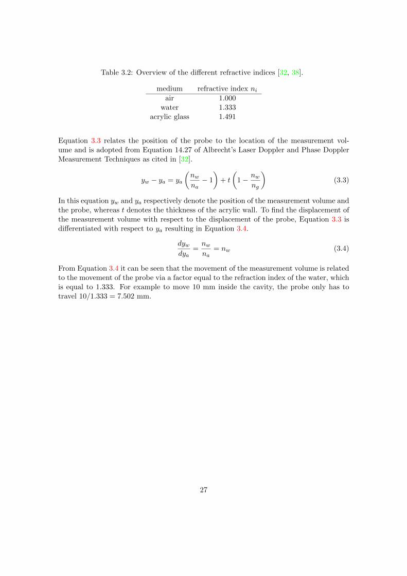
Table 3.2: Overview of the different refractive indices [32, 38].

medium refractive index niair 1.000

water 1.333acrylic glass 1.491

Equation 3.3 relates the position of the probe to the location of the measurement vol-ume and is adopted from Equation 14.27 of Albrecht’s Laser Doppler and Phase DopplerMeasurement Techniques as cited in [32].

yw − ya = ya

(nwna− 1

)+ t

(1− nw

ng

)(3.3)

In this equation yw and ya respectively denote the position of the measurement volume andthe probe, whereas t denotes the thickness of the acrylic wall. To find the displacement ofthe measurement volume with respect to the displacement of the probe, Equation 3.3 isdifferentiated with respect to ya resulting in Equation 3.4.

dywdya

=nwna

= nw (3.4)

From Equation 3.4 it can be seen that the movement of the measurement volume is relatedto the movement of the probe via a factor equal to the refraction index of the water, whichis equal to 1.333. For example to move 10 mm inside the cavity, the probe only has totravel 10/1.333 = 7.502 mm.

27

Chapter 4

Results

The reliability of results obtained by measurements is strongly dependent on the perfor-mance of the equipment used. Unfortunately the LDV equipment used in this researchgave a lot of problems in terms of performance. The number of subsequent measurementsthat could be conducted was limited due to a malfunctioning Bragg cell power supplyunit. This was unable to amplify the 40 MHz shifted beams leaving the Bragg cell enoughto match the required intensity of the unshifted beams, as is shown in Table 3.1. Apartfrom that, the main problem was that it could not power the Bragg cell for longer peri-ods of time. Therefore only measurements could be conducted for short periods of timein the order of a couple of hours. After this it needed to be switched off for at leastan equal amount of time before the measurements could be continued. To give an ideaof the limitation this imposed; Popinhak measured the flow profile in the cavity at ninedifferent heights, each height consisting out of 128 points. Every point was measured foreight minutes. Redoing all of his measurements would take 135 hours of doing non-stopmeasurements. It was simply impossible to exactly redo his measurements. Therefore itwas chosen to measure on a courser grid and also to measure every point only for twominutes or 111 successful particle detections. To guarantee the accuracy of the results,the measurement data is analysed to find a minimum of particle detections necessary.

What became clear after the visit of a specialized external technician was that the opticfibres connecting the beam shifter to the scope were in a very bad condition. In a systemin good condition about 60% of the power generated by the laser is lost in the transmittingoptics. In our LDV setup about 94% is lost. This can not be solved by increasing thepower output of the laser, since also the quality of the laser beam is of influence on theresults. A high quality laser beam will create a well defined (neat) measurement area.When a large part of the signal is lost during transmission, the measurement area will beof lesser quality. This will result in a lower data rate and reliability of the results

28

4.1 Number of particles in the cavity

In previous work there was no notion given regarding the exact amount of particles in thecavity required to do measurements. What was learned from previous executors of theexperiment, was that they used to mix about half a teaspoon of particles with the waterin the cavity. This was copied by us in our first experiments, resulting in a zero data ratefrom the cavity. Since there was data when a wider frequency filter band was reviewed,the calculations used to choose the filter and frequency shift were double checked. Whenthese seemed all correct, it was concluded that the problem must be in the cavity itself,specifically in the amount of particles in the cavity flow.Since there was no signal captured from the cavity, the first conclusion was that the numberof particles had to be to low, so it was increased. The original amount of particles added(half a teaspoon) was weighted and increased. Later also the data rate was tested for loweramounts of particles, denoted small in Table 4.1. These initial experiments (the first fourentries of Table 4.1) gave no clear results on the correct required amount of particles.An overview of all the different variations used is given in Table 4.1. Limited by theaccuracy of the scale initially used, for the majority of the tests it was only possible to dorough estimations of the added amount of particles. This accounts for the first five entriesof Table 4.1.

Table 4.1: Overview of the different amounts of particles used in the cavity in order toobtain data readings.

amount by visual inspection weight [gram] data rate present

normal; half a teaspoon 0.2 ± 0.01 sometimesvery large ± 0.8 no data ratesmall ± 0.1 no data ratesmall ± 0.05 no data ratevery small 0.005 ± 0.0025 steady data ratevery small 0.0068 steady data rate

When the initial experiments gave no useful results, more information on the topic ofcorrect amount of seeding particles was found in the PDPA/LDV operations manual. Inthe manual is stated that the optimal particle density is one particle per measurementvolume [5]. The measurement volume is given in Equation 4.1 which is adopted fromEquation 5.41 from Albrecht’s Laser Doppler and Phase Doppler Measurement Techniquesas cited in [32].

V0 =8π

3

r3wsin θ

(4.1)

In this equation rw is the radius of the laser beam waist and θ is the angle under which theintersecting laser beams cross each other [32]. Filling in these values, which were foundin the FlowSizer software results in a measurement volume of 4.39×10−2 mm3 for theintersecting green bundles and 3.75×10−2 mm3 for the blue bundles.

29

As described in the PDPA/LDV operations manual, the optimal particle density is equalto the inverse of the measurement volume [5]. The particles are assumed to be sphericaland have a radius of 0.25 µm. Using this, the volume of one particle can be calculated.Combined with the known volume of the cavity and particle mass (1.03 kg/dm3), therequired total particle mass for the cavity was calculated to be 0.0072 gram, based onthe measurement volume created by the blue laser bundles and 0.0061 gram for the greenmeasurement volume.

Indeed measurements performed with an added particle mass of 0.005 ±0.0025 gram didresult in a constant data rate. The uncertainty of this number is based on resolution of thescale used resolution, which is 0.01 gram. The procedure to obtain the stated amount ofparticles consisted out of measuring 0.01 gram and adding half of the amount to the cavity.When more accurate weight measurements where possible, experiments were conductedwith a well defined 0.0068 gram of particles. This showed very good results in terms ofdata rate.

4.2 Number of data readings

An important parameter in terms of efficiency is the number of data readings from par-ticles passing through the measurement volume required to obtain a reliable averagedvelocity. This was studied by doing measurements for a longer period of time at the sameposition and calculating the average velocity per number of measurements. The data usedto create the velocity profiles in Section 4.3 is analysed in the same way to ensure thatreliable results are presented there.

Shown in Figure 4.1 is the typical behaviour of the averaged value of the vertical velocityper number of data measurements at a certain position. The two horizontal lines indicatethe boundaries of the rounded average over the total set of velocity data.The convergence of the averaged value of the velocity near the cold wall at 0.7 cavityheight is shown in Fig. 4.2. The data used to create this graph is also used to createthe velocity profile near the cold wall in Figure 4.3c. The velocities are averaged after xnumber of measurements and rounded to the order of 0.1 mm/s. Note that the absoluterounded velocities are shifted in this graph. Of importance here is the change in roundedvelocity with increasing number of data counts.

4.3 Velocity profiles

Velocity measurements were performed near the hot and the cold wall at different heightsas described in Section 3.2. The first set of measurements was performed on the samefine grid as Popinhak used, however using incorrect filter and downmixing settings. Thisresulted in only positive velocity measurements, since the negative measurements were fil-tered from the signal. Measurements with the correct settings were due to time limitationsperformed on a less fine grid with a spacing of 1 mm. The maximum data count was set

30

0 50 100 150 200 2503.35

3.4

3.45

3.5

3.55

3.6

3.65

3.7

3.75

3.8

3.85

number of data counts

ave

rag

e v

elo

city [

mm

/s]

Figure 4.1: The averaged value of the vertical velocity per number of data measurementsand the boundaries of the rounded average velocity.

0 10 20 30 40 50 60 70 805

6

7

8

9

10

11

12

13

14

number of data counts

sh

ifte

d a

ve

rag

e v

elo

city [

mm

/s]

Figure 4.2: Shifted rounded average velocities near the cold wall at 0.7 cavity height.

at 111 or two minutes of measurements per measurement location for reasons explainedin Section 5.2.

Shown below in Figure 4.3 are the velocity profiles from the measurements near the hotand the cold wall for a cavity height of 0.3 and 0.7 times the total height. Also the results

31

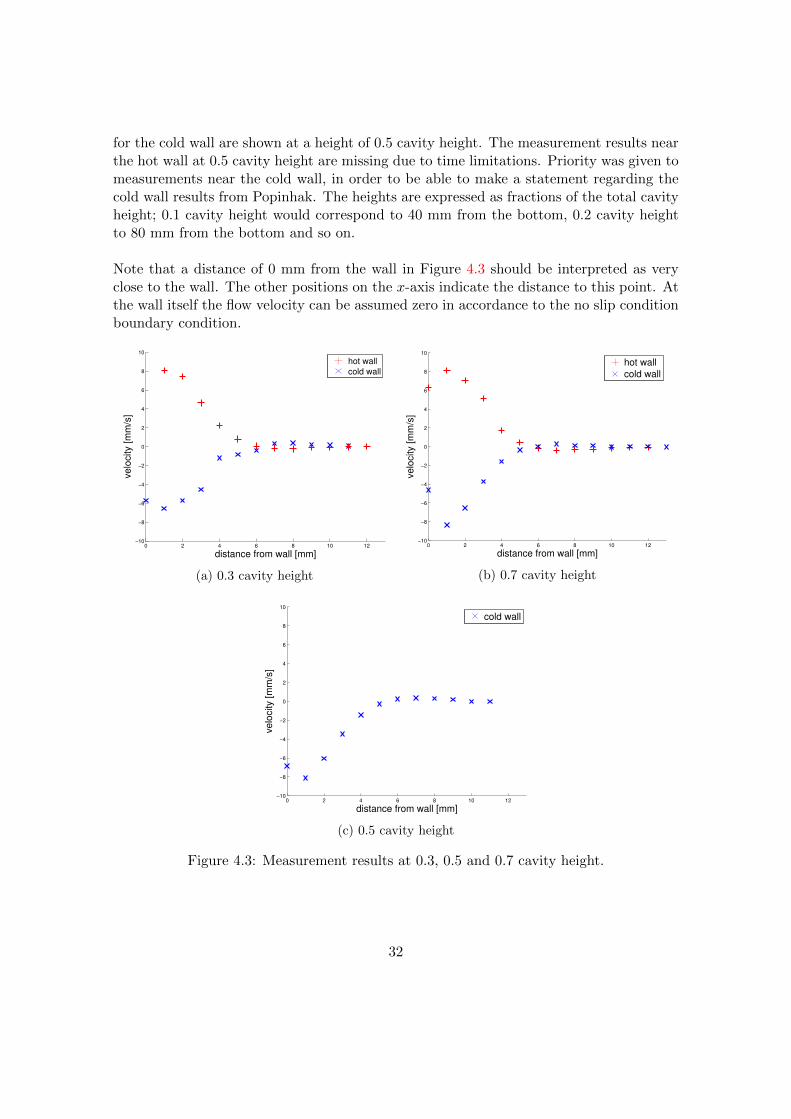
for the cold wall are shown at a height of 0.5 cavity height. The measurement results nearthe hot wall at 0.5 cavity height are missing due to time limitations. Priority was given tomeasurements near the cold wall, in order to be able to make a statement regarding thecold wall results from Popinhak. The heights are expressed as fractions of the total cavityheight; 0.1 cavity height would correspond to 40 mm from the bottom, 0.2 cavity heightto 80 mm from the bottom and so on.

Note that a distance of 0 mm from the wall in Figure 4.3 should be interpreted as veryclose to the wall. The other positions on the x-axis indicate the distance to this point. Atthe wall itself the flow velocity can be assumed zero in accordance to the no slip conditionboundary condition.

0 2 4 6 8 10 12−10

−8

−6

−4

−2

0

2

4

6

8

10

distance from wall [mm]

ve

locity [

mm

/s]

hot wall

cold wall

(a) 0.3 cavity height

0 2 4 6 8 10 12−10

−8

−6

−4

−2

0

2

4

6

8

10

distance from wall [mm]

velo

city [m

m/s

]

hot wall

cold wall

(b) 0.7 cavity height

0 2 4 6 8 10 12−10

−8

−6

−4

−2

0

2

4

6

8

10

distance from wall [mm]

ve

locity [

mm

/s]

cold wall

(c) 0.5 cavity height

Figure 4.3: Measurement results at 0.3, 0.5 and 0.7 cavity height.

32

Chapter 5

Conclusions and discussion

The goals for this internship were to perform maintenance to get the setup back in op-erational condition, to redo the measurements performed by Popinhak and try to findan explanation for his somewhat anomalous results. The maintenance required a lot oftime since the measurement equipment turned out to be in a lesser state than expected.Therefore the number of measurements that could be conducted was limited. Neverthelesssome important conclusions can be drawn from the results.

5.1 Number of particles in the cavity

Based on the experimental results presented in Table 4.1, it is concluded that the amountof added polystyrene seeding particles in the flow is an important parameter in obtainingreliable results. The correct amount was calculated assuming that ideally at all times onlyone particle is present in the measurement volume. For the measurement volume createdby the intersecting green laser bundles this was calculated to be 0.0061 gram of particles.For the blue bundles this is 0.0072 gram. Indeed experiments with a added amount of0.0068 gram particles showed a steady data rate.

The question that rises based on these results is why Popinhak did find a (high) datarate, whilst it can be safely assumed that he used a particle density much higher than iscalculated as being the optimum. In the master’s thesis written by Popinhak (as citedin [3]) no mention is given of the amount of particles added to the cavity. Only afterconsultation with one of his temporary co-workers (Chris Willemsen) it was found thathe used about half a teaspoon of particles. Clearly, the amount of particles was not foundto be of influence at that time. One possible explanation for this is that the LDV mea-surement equipment was in a better condition at the time when Popinhak performed hismeasurements. Therefore the amount of particles might have been of lesser importanceand the equipment was better capable of handling more particles in the measurement vol-ume at the same time.

What also should be taken into account is that when larger amounts of particles are used,

33

not all the particles dissolve in the water. Large amounts of particles are seen to stick tothe front, back and top walls of the cavity. This means that actually lower amounts ofparticles are dissolved than is being stated or assumed. This is also something to keep inmind when adding the calculated very low amounts of particles, since there will always besome particles that are not dissolved.

5.2 Number of data readings

From Figure 4.1 can be seen that after a small number of measurements, the averagedvelocity is already close to the final averaged velocity within a range of 0.1 mm/s. Basedon these results it is concluded that the average value after 100 measurements is accurateenough to be used in a velocity flow profile. To be on the safe side, a maximum numberof 111 data measurements per measurement position is used in the experiments. In orderto obtain insight in the flow profile, an error value of 0.1 mm/s is tolerated in this report.Based on Figure 4.1 the error will be smaller than 0.1 mm/s after 100 measurements.Thereby Figure 4.2 shows stable convergence which leads to the conclusion that the num-ber of measurements chosen is sufficient and the results are reliable.

5.3 Velocity profiles

Although the measurements were not performed on a very fine grid, nor with the highestpossible accuracy, some important conclusions can be drawn. The most important conclu-sion is that the flow profiles near the hot and cold wall look very symmetric. This includesthe small backflow (sign change of velocity) when moving further from the wall.The velocity profiles found in this research show near resemblance to the results fromthe numerical work by Trias et al. [2]. This is mainly seen in the symmetry between theflow profiles near the hot and the cold wall that can also be seen in Figure 2.3, which isadopted from the work by Trias et al.. Thereby, the backflow observed in Figure 4.3 isalso reported near both the hot and cold wall side by Trias et al. [2]. The vortices in thetime averaged flow as described by Trias et al. in the top and bottom corner of the hot,respectively cold wall are however not observed in this research [2]. Perhaps when a finergrid is used combined with measurements of the horizontal velocities it is possible to makea statement regarding this.

Saury et al. performed measurements for different Rayleigh numbers [4]. In contrary totheir results we did find a backflow at the cold wall side, whereas Saury et al. only foundthis phenomena at the hot wall side [4]. The Rayleigh numbers used by Saury et al. arehigher than the one used in this research (4.0 ×1010 - 1.2×1011 versus 1.14×1010), but itis unlikely that this is causing the difference in results. Apart from this, no other signif-icant differences are found when comparing the results from Saury et al. with the resultspresented in Section 4.3.

34

A lot of similarities are present between the results from different authors pointed outin this section and the results presented in Section 4.3. Therefore it is concluded thatthe measurements were performed accurately enough and the results are valid to drawconclusions from.

The most important motive for the research presented here, was to obtain better insightin the results found by Popinhak using the same cavity [3]. The literature research showedsome similarities in terms of the secondary rotary flows found by Popinhak in the top andbottom corners of the hot, respectively cold wall. His results seem to be in accordancewith the corner vortices found in the numerical study by Trias et al. [2]. The same goesfor Popinhak’s flow profiles near the hot wall. These show resemblances to the profilesfound by both Trias et al. (as cited in [2]) and Saury et al. [4]. Important characteristicssuch as the shape of the flow profile and the relative size of the backflow match closelywhen they are compared.

A lot of confusion existed however regarding the flow profiles near the cold wall as foundby Popinhak. These feature an almost sinusoidal velocity distribution due to an unpropor-tionally large backflow. Also the maximum absolute velocities found near the cold wall aremuch lower than would be expected. These kind of results were not found in the literaturestudy and also did not show up in the experimental work presented in this report.One major difference in how the experiments were conducted by Popinhak was in the num-ber of particles being added to the water in the cavity. This can however be disregardedas being the cause of the peculiar flow profile found near the cold wall, since this shouldalso have influenced the flow or measurements near the hot wall.

Careful inspection of the settings files as used by Popinhak to perform his measurementsrevealed that he made a questionable choice when selecting the frequency filter and down-mixing frequency. In the vast majority of his measurements, a frequency filter rangingfrom 0.3 to 3.0 kHz with a downmix value of 39.999 MHz was programmed. Using Eq. 2.18,the Doppler frequency fdoppler can be determined as shown in Equation 5.1.

fdoppler = ffilter + fdownmix − fshift (5.1)

Filling in for the filter and downmix frequency (Popinhak used 0.3 - 3 kHz and 39.999MHz) as well as the frequency of the Bragg cell used (40 MHz), the range of fdoppler isfound to be between -0.7 and 2 kHz. Using Eq. 2.17 this results in a velocity range between-2.6 and 7.5 mm/s for the green laser light and between -2.5 and 7.1 mm/s for the bluelaser. What can be concluded from this is that Popinhak never was able to find a correctvertical flow profile near the cold wall, since the negative velocities below -2.6 mm/s werefiltered from his results.

Although regarding this, it is still very strange that his velocity profiles displays the sinu-soidal behaviour close to the cold wall. More sense would make a normal velocity profilebeing cut off at -2.6 mm/s, resulting in some sort of a negative plateau shape. Thereby,

35

the measurement from Popinhak at 0.9 cavity height, as shown in Figure A.1i, shows amaximum negative velocity of -3 mm/s at the cold wall side. Theoretically, with the abovespecified filter and downmixing frequency, the system should be unable to capture this.

Popinhak gives no information or motivation on the settings used for the filter and down-mixing in his thesis [3]. Therefore, based on the abnormal velocity profiles and the argu-mentation given here, his results in the form of observations, flow profiles and conclusionsbased on LDV measurements near the cold wall side can be regarded as incorrect.

The flow profiles from Popinhak near the hot wall do not show any kind of peculiarbehaviour and do fit within the filter and downmixing used. Therefore it is believed thatthese results are reliable. Apart from the LDV measurements, Popinhak also performedmeasurements using PIV (Particle Image Velocimetry). No research has been conductedto get more insight in the PIV results from Popinhak, so no statements can be maderegarding these measurements, results or conclusions drawn based on this.

5.4 Recommendations for further research

Complete flow profile It would be good to have a complete overview of the flowprofile at different heights in the cavity. This should contain the horizontal flow velocitiesas well. Using this data, a more quantitative analysis can me made of the results obtainedby Popinhak. This would make it as well possible to further comment on the efficiencyof the measurements; is the accuracy indeed assured when less data is used to calculatethe averaged velocity. In order to obtain these results, measurements on a more refinedgrid have been prepared. These measurements can be carried out by the three bachelorstudents working in the same lab. Based on their results, an analysis can be made ofwhich areas in the cavity display interesting flow features. Near the vicinity of these areasmore measurements can be conducted on an even finer grid.

Change Rayleigh number A new set of measurements can be relatively easy obtainedby changing the Rayleigh number. The Rayleigh number is directly related to the temper-ature difference between the hot and the cold wall. For instance temperature differencesof 8.8 degree Celsius and 26.4 degree Celsius match the Rayleigh numbers of 1×1010 and3×1010 as used in the numerical study by Trias et al. [2, 14]. Using these temperature dif-ferences it might be able to check the results by Trias et al., who showed that the point atwhich the boundary layer separates moves upstream with increasing Rayleigh number [2].This can be seen in Figure 2.3, which is adopted from the work by Trias et al. as citedin [2].

Detection of vorticity To get more out of the obtained data, the standard deviationof the velocity measurements at a single position should be studied, to find if a connec-tion exists with the vorticity at that position. In this research only time averaged flows

36

are studied, but with this connection it is also possible to make some comments on theinstantaneous velocity field using the same datasets.

5.5 Recommendations for the lab

Maintenance of measurement equipment As servicing showed, the LDV equipment(beam separator, optic cables, couplers and scope) is in need of some extensive maintenanceand calibration. Advised by the service engineer was to send everything back to themanufacturer in order to take care of all shortcomings. This would probably be expensiveand since it is possible to perform, although limited, measurements with the equipment,the advice of minimal required action is to replace the Bragg cell amplifier for reasonsexplained in Section 4. The amplifier has been replaced before, probably somewhere in2012, judging on the inscription on an old amplifier found in the lab. This would requirecontacting TSI (the manufacturer), since it is very difficult to find specifications or resellersfor the Bragg cell amplifier. The visiting service engineer had no knowledge of whatsoeveron the specifications of this amplifier. When contact is established with TSI, informationcan be exchanged on the efficiencies of the transmitting optics. Based on this informationTSI will probably give an advice as well.

Electrical sockets The multiphase plug powering the laser is positioned directly underthe return faucet for the cooling water. The first time the cooler was switched on aftera long period of rest the connection was leaking. This was repaired, but it is stronglyadvised to review the possible dangers caused by this arrangement.

37

Acknowledgements

It is both challenging and exciting to find and work on an internship abroad. Apart fromthe practical matters, there are also cultural differences to overcome. Luckily, there arealways people who are willing to make life more easy.

First of all I would like to thank professor Harry Hoeijmakers from the University ofTwente. He supported my worldly adventures and used his network of contacts to findme an assignment in Brazil. My professor in Brazil who I would like to thank is professorCesar Deschamps. During my first few weeks he helped me to get settled and made sure Ireceived help from Nara Santos in managing Brazil’s bureaucracy. I am also very gratefulfor the faith and freedom he gave me in organizing my work in the lab. Every time Icame for help or with new ideas, professor Deschamps took this very serious, which issomething I really appreciate. He explained this to me as resulting from having such goodexperiences with other students from the University of Twente.

The three students working with me were Heitor Paes de Andrade, Domicio Moura Lopesand Marcelo Ruaro Bortoli. Apart from helping me with my work, they also made that Ihad a great time working in the lab. After three months we said goodbye as friends and Ihope to meet them again some day.

My brother Jan-Willem Bullee helped me with editing this report. His critical notes onboth my writing and the form of the report were of great help in creating this final version.

38

Bibliography

[1] S. Xin and P Le Quere. Direct numerical simulations of two-dimensional chaoticnatural convection in a differentially heated cavity of aspect ratio 4. Journal of FluidMechanics, 304:87–118, 1995.

[2] F. X. Trias, A. Gorobets, M. Soria, and A. Oliva. Direct numerical simulation of adifferentially heated cavity of aspect ratio 4 with Rayleigh numbers up to 10×1011

Part I: Numerical methods and time-averaged flow. International Journal of Heatand Mass Transfer, 53(4):665–673, January 2010.

[3] A. R. Popinhak. Investigacao experimental da conveccao natural terbulenta em umacavidade com paredes verticais a diferentes temperaturas e razao de aspecto 4. Mas-ter’s thesis, Universidade Federal de Santa Catarina, 2013.

[4] D. Saury, N. Rouger, F. Djanna, and F. Penot. Natural convection in an air-filled cav-ity: Experimental results at large Rayleigh numbers. International Communicationsin Heat and Mass Transfer, 38(6):679–687, 2011.

[5] Phase Doppler Particle Analyser (PDPA) / Laser Doppler Velocimeter (LDV). TSIIncorporated, revision d edition, 2005.

[6] Y. A. Cengel. Heat Transfer: A Practical Approach.

[7] F. P. Incropera and T. L. Bergman. Fundamentals of Heat and Mass Transfer. 2011.

[8] Turbulent natural convection of air in a non-partitioned or partitioned cavity withdifferentially heated vertical and conducting horizontal walls. Experimental Thermaland Fluid Science, (29):137 – 157, 2009.

[9] H. Benard. Les Tourbillons cellulaires dans une nappe liquide transportant de lachaleur par convection en regime permanent. PhD thesis, 1901.

[10] P. K. Kundu, I. M. Cohen, and D. R. Dowling. Fluid Mechanics. 5 edition, 2012.

[11] The Engineering Toolbox, http://www.engineeringtoolbox.com, visited 12-03-2014.

[12] UCLA Hall of Pioneers, http://www.seas.ucla.edu/jht/pioneers/pioneers.html, vis-ited 21-03-2014.

39

[13] J. Holman. Heat Transfer. 2009.

[14] F. X. Trias, A. Gorobets, M. Soria, and A. Oliva. Direct numerical simulation of adifferentially heated cavity of aspect ratio 4 with Rayleigh numbers up to Part II:Heat transfer and flow dynamics. International Journal of Heat and Mass Transfer,53(4):674–683, 2010.

[15] R. B. Bird, W. E. Stewart, and E. N. Lightfoot. Transport Phenomena, Revised 2ndEdition. 2nd edition, 2006.

[16] T. L. Lee and T. F. Lin. Transient three-dimensional convection of air in a differen-tially heated rotating cubic cavity. International Journal of Heat and Mass Transfer,39(6):1243–1255, 1996.

[17] W. H. Leong, K. G. T. Hollands, and A. P. Brunger. Experimental Nusselt numbersfor a cubical-cavity benchmark problem in natural convection. International Journalof Heat and Mass Transfer, 42(11):1979–1989, 1999.

[18] Y. T. Ker and T. F. Lin. A combined numerical and experimental study of airconvection in a differentially heated rotating cubic cavity. International Journal ofHeat and Mass Transfer, 39(15):3193–3210, 1996.

[19] D. Dabiri. The Effects of Forced Boundary Conditions on Flow Within a Cubic CavityUsing Digital Particle Image Thermometry and Velocimetry ( DPITV ). ExperimentalThermal and Fluid Science, 13:349–363, 1996.

[20] W. Schopf and J. C. Patterson. Visualization of natural convection in a side-heatedcavity: Transition to the final steady state. International Journal of Heat and MassTransfer, 39(16):3497–3509, 1996.

[21] M. A. H. Mamun, W. H. Leong, K. G. T. Hollands, and D. A. Johnson. Cubical-cavitynatural-convection benchmark experiments: an extension. International Journal ofHeat and Mass Transfer, 46(19):3655–3660, 2003.

[22] W. Nusselt. Die Warmeleitfahigkeit von Warmeisolierstoffen. Mitteilungen uberForschungsarbeiten auf dem Gebiete des Ingenieurwesens. 1909.

[23] E. R. G. Eckert and W. O. Carlson. Natural convection in an air layer enclosedbetween two vertical plates with different temperatures. International Journal ofHeat and Mass Transfer, 2:105–120, 1961.

[24] G. K. Batchelor. Heat Transfer by Free Convection across a Closed Cavity betweenVertical Boundaries at Different Temperatures. Quarterly of Applied Mathematics,12:209–233, 1954.

[25] F. Penot, A. N’Dame, and P. Le Quere. Investigation of the route to turbulencein a vertical differentially heated cavity. Proceedings of the 6th International HeatTransfer conference, pages 417 – 422.

40

[26] F. Penot, O. Skurtys, and D. Saury. Preliminary experiments on the control ofnatural convection in differentially-heated cavities. International Journal of ThermalSciences, 49(10):1911–1919, 2010.

[27] R. J. A. Janssen, R. A. W. M. Henkes, and C. J. Hoogendoorn. Transition to time-periodicity of a heated cavity. International Journal of Heat and Mass Transfer, 36(11):2927–2940, 1993.

[28] R. J. A. Janssen and R. A. W. M. Henkes. Instabilities in three-dimensionaldifferentially-heated cavities with adiabatic horizontal walls. Physics of Fluids, 8(1), 1996.

[29] G. Labrosse, E. Tric, H. Khallouf, and M. Betrouni. A Direct (Pseudo-Spectral) Solverof the 2D/3D Stokes Problem: Transition To Unsteadiness of Natural-ConvectionFlow in a Differentially Heated Cubical Cavity. Numerical Heat Transfer, Part B:Fundamentals, 31(3):261–276, 1997.

[30] F. X. Trias, M. Soria, A. Oliva, and C. D. Perez-Segarra. Direct numerical simulationsof two- and three-dimensional turbulent natural convection flows in a differentiallyheated cavity of aspect ratio 4. Journal of Fluid Mechanics, 586:259–293, 2007.

[31] R. J. A. Janssen and R. A. W. M. Henkes. Influence of Prandtl number on instabilitymechanisms and transition in a differentially heated square cavity. Journal of FluidMechanics, 290:319–344, 1995.

[32] H. E. Albrecht, M. Borys, N. Damaschke, and C. Tropea. Laser Doppler and PhaseDoppler Measurement Techniques. 2003.

[33] The Prospector Materials Database. Acrylic Typical Properties Generic Acrylic(PMMA), http://plastics.ides.com/generics/3/c/t/acrylic-properties-processing, vis-ited 11-03-2014.

[34] TSI webinar notes cq powerpoint presentiation on LDV PDPA Optics,ftp://ftp.tsi.com/pub/fluid

[35] TR/TM Series Fiberoptic Probes Manual. TSI, Revision C edition, January 2007.

[36] TSI website, http://www.tsi.com/3-axis-traverse-system/, visited 23-04-2014.

[37] TR/TM Series Fiberoptic Probes Owner’s Manual. TSI Incorporated, revision c edi-tion, 2007.

[38] E. Hecht. Optics. 4th edition, 2003.

41

Appendix A

Measurement results by Popinhak

(a) 0.1 cavity height (b) 0.2 cavity height

(c) 0.3 cavity height (d) 0.4 cavity height

Figure A.1: First part of the measurement results by Popinhak.

42

(e) 0.5 cavity height (f) 0.6 cavity height

(g) 0.7 cavity height (h) 0.8 cavity height

(i) 0.9 cavity height

Figure A.1: Second part of measurement results as presented by Popinhak in his master’sthesis as cited in [3]. Plotted are the vertical flow velocities near both the hot and the coldwall as a function of the distance to the corresponding wall. Measurements where per-formed at different heights relative to the bottom of the cavity. The heights are expressedas fractions of the total cavity height; 0.1 cavity height corresponds to 40 mm from thebottom, 0.2 cavity height to 80 mm from the bottom and so on.