Internet Traffic Engineering by Optimizing

OSPF Weights

Bernard Fortz (Université Libre de Bruxelles) Mikkel Thorup (AT&T Labs-Research)

Presented by : Mordo Shalom

The Routing (Load) Optimization Problem

Input: A directed graph G=(N,A) A demand function A capacity function A cost function

is the cost incured by a routing with load l on an arc with capacity c.

An instance is given by a triple (G,D,c), is known a priori.

:D N N R

:c A R

:R R R

( , )l c

The Objective Any routing R, implies a load function

on the edges The cost induced by this load is:

The total cost of the routing

The Objective :Find a routing R such that is minimized.

:l A R

( ( )) ( ( ), ( ))al a l a c a

( ( ))R aa A

l a

R

OSPF Routing The network administrator assigns

a weight to each arc (link): OSPF routes packets on the

shortest path induced by the function w.

When there are multiple shortest paths packets are routed on each of them with equal probability.

:w A R

The OSPF Routing Optimization Problem

Find a weight function such that . is minimized.

:w A R

( )OSPF w

The cost function For each arc a is a piecewise-

linear non decreasing function. In fact any convex function would do

the job.

a

1 0 / ( ) 1/ 3

3 1/ 3 / ( ) 2 / 3

10 2 / 3 / ( ) 9 /10'( )

70 9 /10 / ( ) 1

500 1 / ( ) 11/10

5000 11/10 / ( )

a

for x c a

for x c a

for x c ax

for x c a

for x c a

for x c a

0

10

20

30

40

50

60

70

0 1/3 c(a)

2/3c(a)

0.9c(a) c(a) 1.1c(a)

Cost

The Cost Function

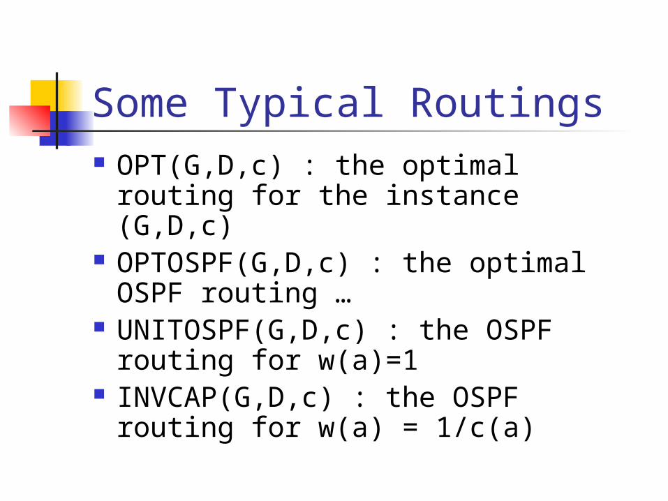
Some Typical Routings OPT(G,D,c) : the optimal routing

for the instance (G,D,c) OPTOSPF(G,D,c) : the optimal OSPF

routing … UNITOSPF(G,D,c) : the OSPF

routing for w(a)=1 INVCAP(G,D,c) : the OSPF routing

for w(a) = 1/c(a)

A normalized cost d1(s,t) is the length of the shortest

path from s to t where w(a)=1 for all a.

When then , in particular .

The cost of the OSPF routing under this setting:

The above value is called

, ( )a A c a ( )ax x

( ( )) ( )al a l a

1( , , ) ( , ) ( , )UNITOSPF a

G D D s t d s tl

( , )UNCAP

G D

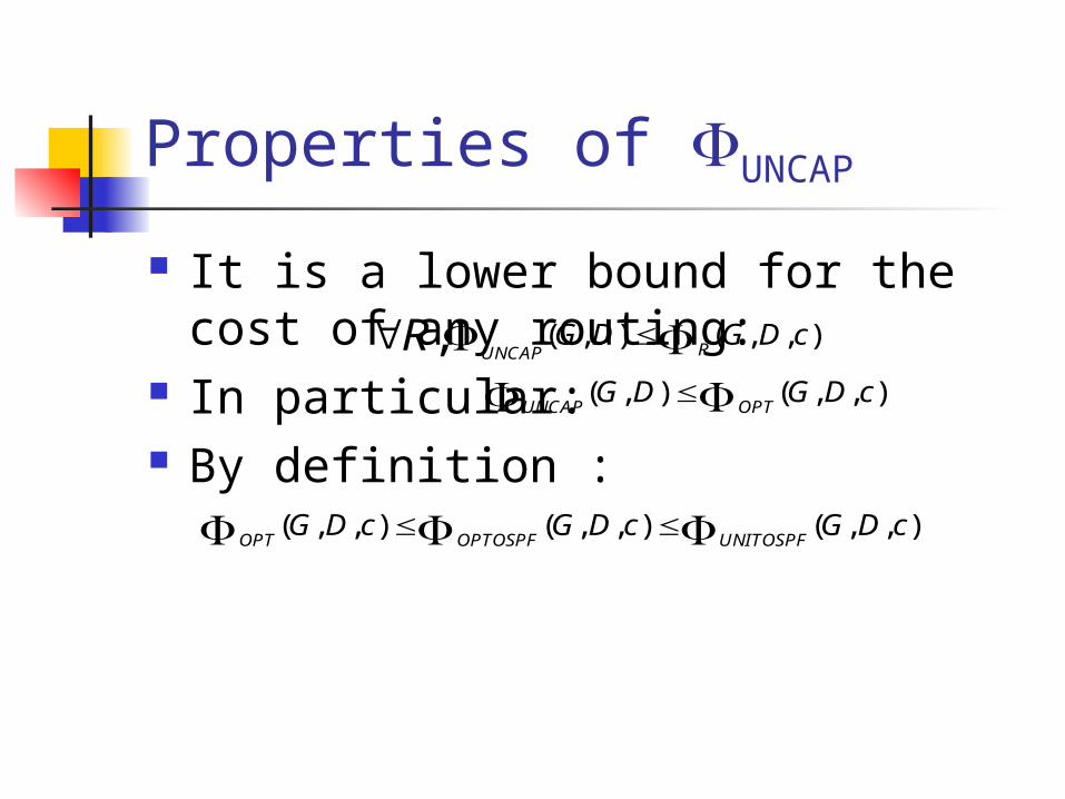
Properties of UNCAP

It is a lower bound for the cost of any routing:

In particular: By definition :

( , ) ( , , ), RUNCAPG D G D cR ( , ) ( , , )

UNCAP OPTG D G D c

( , , ) ( , , ) ( , , )OPT OPTOSPF UNITOSPF

G D c G D c G D c

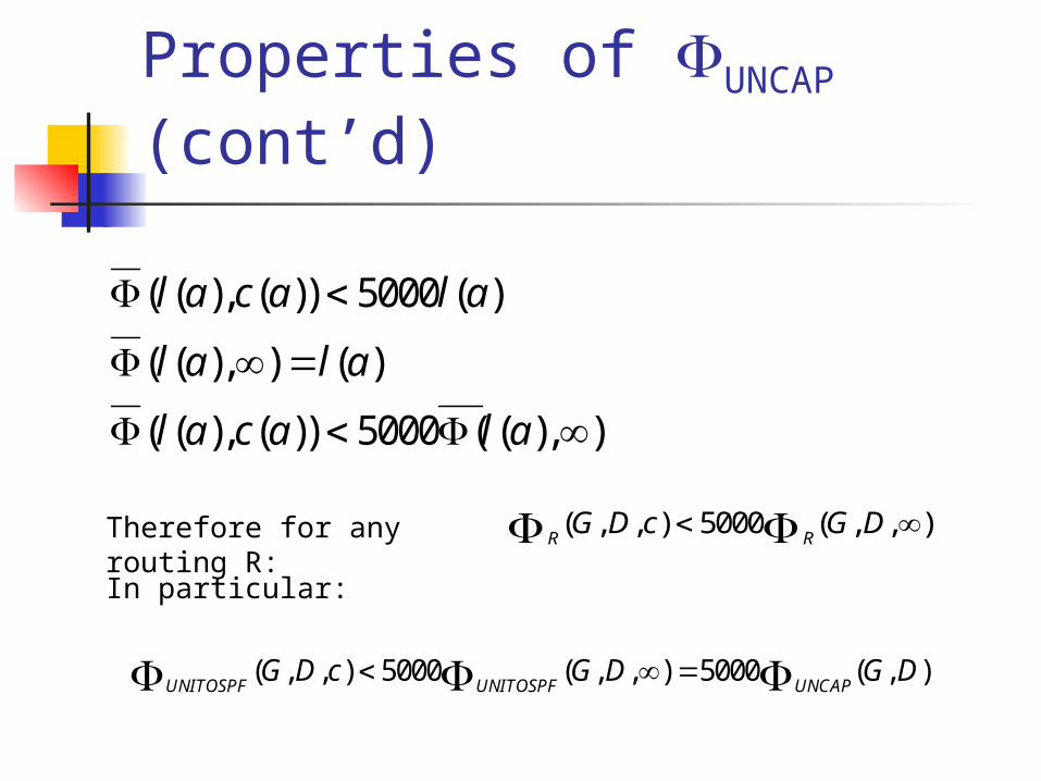
Properties of UNCAP (cont’d)

( ( ), ( )) 5000 ( )

( ( ), ) ( )

( ( ), ( )) 5000 ( ( ), )

l a c a l a

l a l a

l a c a l a

Therefore for any routing R:

( , , ) 5000 ( , , )R RG D c G D

In particular:

( , , ) 5000 ( , , ) 5000 ( , )UNITOSPF UNITOSPF UNCAP

G D c G D G D

Properties of UNCAP (cont’d)

Summarizing:

*( , , ) ( , , ) / ( , )R R UNCAPG D c G D c G D We

define:

( , ) ( , , ) ( , , )

( , , ) ( , , ) 5000 ( , )UNCAP UNITOSPF OPT

OPTOSPF UNITOSPF UNCAP

G D G D G D c

G D c G D c G D

* * *1 ( , , ) ( , , ) ( , , ) 5000

OPT OPTOSPF UNITOSPFG D c G D c G D c

We have:

The Main Results For each n there is an instance such that

OPT(G,D,c) can be found in polynomial time.

To find OPTOSPF is NP-Hard, moreover it is NP-Hard to find a 1.77-approximation to OPTOSPF

A Local Search Heuristic to approximate OPTOSPF

lim 5000OPTOSPF

nOPT

The first result

The family of instances ( , , )nn nG cD

s

1

2

3

n

t

n2-2

n2-4

n2-3

n2-n-1

3

3

3

3

3n3n3n

,( , )

0

n x s y tD x y

otherwise

3

33

3

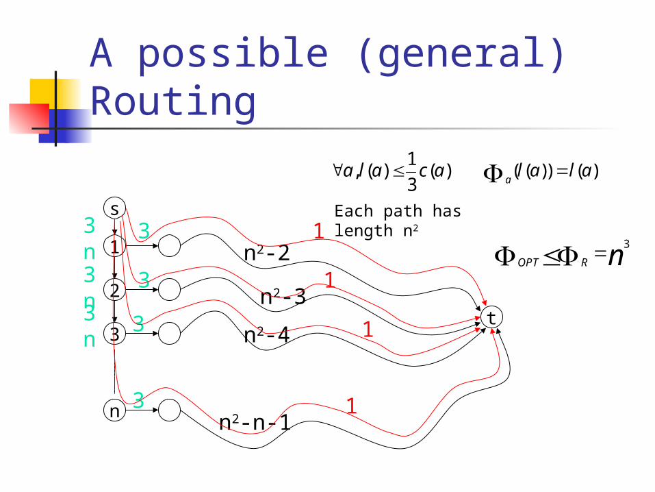
A possible (general) Routing

s

1

2

3

n

t

n2-2

n2-4

n2-3

n2-n-1

3

3

3

3

3n3n3n

1

1

1

1

1, ( ) ( )

3a l a c a ( ( )) ( )

al a l a

Each path has length n2

3

OPT R n

A typical OSPF routing

s

1

2

3

n

t

n2-2

n2-4

n2-3

n2-n-1

3

3

3

3

n/2

19468, 3.3 ( ( )) 5000 ( ) ( ) 5000 ( ) (1)

32i a

ni l a l a c a l a O

3lim 5000OSPF

n n

n/8

n/4

n

n/2

n/4

32 2( )(5000 (1)) 5000 ( )

2 2i ii

ni O O nnn

The Second Result There is a polynomial time

algorithm to find OPT(G,D,c)

Proof: Define as the part of the demand D(s,t) routed through arc a. Formulate the problem as a Linear Programming problem.

( , )s t

af

The Linear Program for OPT

( , ) ( , )

( , ) ( , )( , ) ( , )

( , )

( , )

( , )

. .

( , )

, , ( , )

0

,

,

, (2 / 3) ( )

, (16 / 3) ( )

...

, , 0

310

aa A

s t s t

x y y zx y A y z A

s t

a as t

a a

a a

a a

s t

aaa

Minimize

s t

D s t if y s

y s t N D s t if y t

otherwise

a A

a A

a A c a

a A c a

f f

fl

lll

f l

A Local Search Heuristic(HEUR)

W={1,2,…,wmax} is the set of all possible weights.

The search is on all possible functions (vectors)

Start with a random vector Do {

} Until x meets some optimality criteria

: ( )A

w A W WA

RANDx w W

( ( ) )A

x SEARCH x W N

The Neighborhood Structure if x’ can be obtained from

x by one of the following two: Single weight change:

Choose an arc and change its weight There are |A|x(|W|-1) such neighbors

Evenly balance flows: Choose a node x and a destination t and

balance There are |N|x(|N|-1) such neighbors

' ( )x xN

Evenly Balancing Flows

x

x1

x2

x3

xp

t

P1

P2

P3

Pp

*1 max{ ( ) |1 }

iw i pw P

*( )' iiww w P Every xi is on a shortest path

to t.

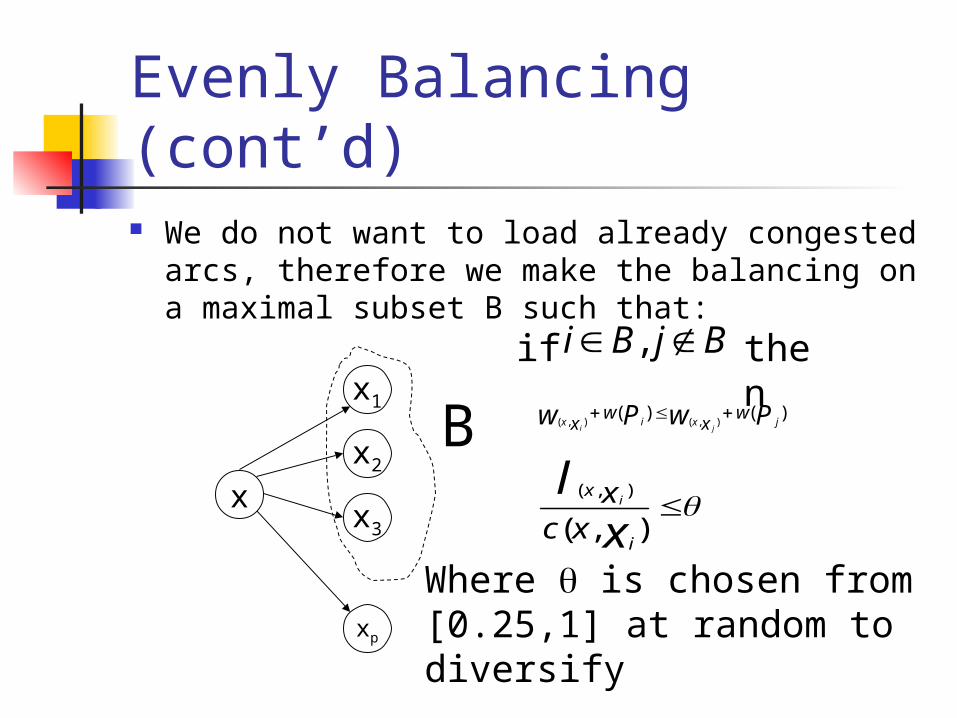
Evenly Balancing (cont’d) We do not want to load already congested

arcs, therefore we make the balancing on a maximal subset B such that:

x1

x2

x3

xp

x

B

,i B j B

( , ) ( , )( ) ( )

i ji jx x

w wx xw wP P

if then

( , )

( , )i

x

i

xc x

lx

Where is chosen from [0.25,1] at random to diversify

Evenly Balancing (cont’d) We do not want w’ > wmax, therefore we

impose on B the following additional condition:

max

( ) { ( ) | }

max ( ) min ( ) 1i

W B w i B

W B W B

Pw

Local Search Do {

} Until x is a local minimum SEARCH returns x’ s.t. cost(x’)<cost(x) Problem: A local minimum may be far

from global minimum Solution: Allow non-improving moves

( ( ))x SEARCH x N

Local Search (cont’d) Problem: We may encounter cycles. Solution: Tabu Search (maintain a

tabu list of the attributes of visited points)

HEUR uses a hash function h and a table T with 1 bit for each possible value of h.

If T(h(x’))=true, SEARCH does not return x’.

Local Search (cont’d) Problem: Duplicate neighbors due

to the complex neighborhood structure.

Solution: SEARCH maintains an internal hash table T’.

If T’(h(x’))=true, SEARCH does not evaluate the cost of x’.

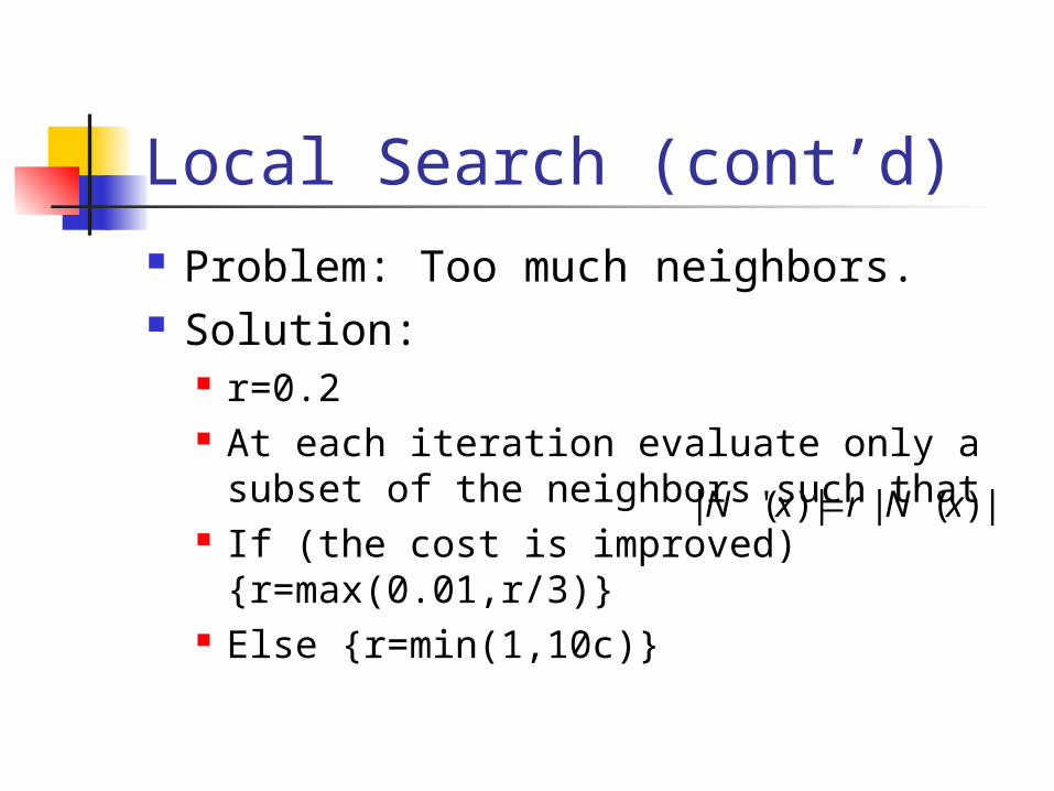
Local Search (cont’d) Problem: Too much neighbors. Solution:

r=0.2 At each iteration evaluate only a

subset of the neighbors such that If (the cost is improved)

{r=max(0.01,r/3)} Else {r=min(1,10c)}

| '( ) | | ( ) |x r xN N

Diversification Choose at random as described

before. If cost is not improved for 300

iterations, perturb x by adding a random perturbation, selected at random from [-2,2] to %10 of the weights.

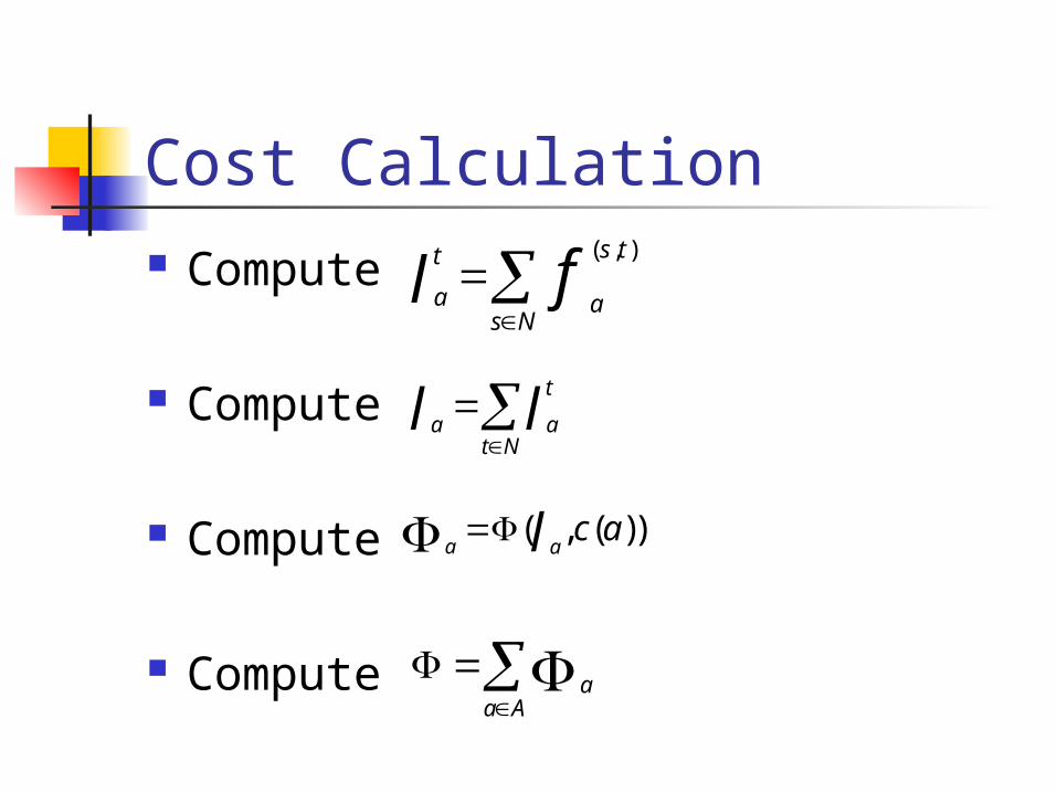
Cost Calculation Compute Compute

Compute

Compute

( , )s tt

a as Nfl

t

a at N

l l

( , ( ))a a

c al

aa A

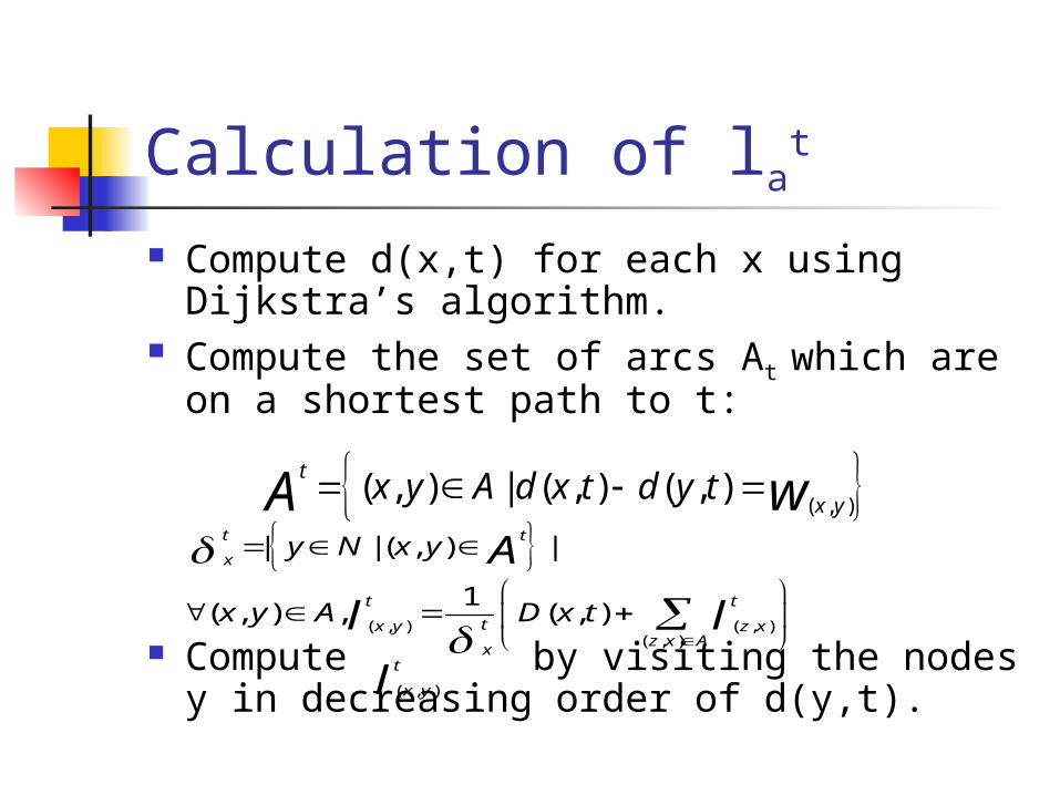
Calculation of lat

Compute d(x,t) for each x using Dijkstra’s algorithm.

Compute the set of arcs At which are on a shortest path to t:

Compute by visiting the nodes y in decreasing order of d(y,t).

( , )( , ) | ( , ) ( , )

t

x yx y A d x t d y t wA

| | ( , ) |t t

xy N x y A

( , ) ( , )( , )

1( , ) , ( , )

t t

tx y z xz x A

x

x y A D x tl l

( , )

t

x yl

Recalculation of lat

At each iteration the calculation should be repeated due to the changes in the weights: Recalculation of d(x,t) : At each

iteration only edges emanating from a single node are changed.

We use the Ramalingam & Reps algorithm (Dijkstra on dynamic graphs). Its running time is proportional to the number of edges incident to nodes for which d(x,t) changed.

Recalculation of lat (cont’d)

In the same manner At’ is calculated for edges incident to nodes x with d(x,y) changed.

Maintain a set M of critical nodes: Initially M contains all the nodes with

incident edges in i.e. the nodes with d(x,y) changed and their neighbors.

't t

A A

Numerical Results Two Additional routings are measured,

along the others: L2OSPF : weights proportional to the

Euclidean distance between nodes. RANDOMOSPF : Weight are assigned

randomly (The first step of HEUR). The algorithms are compared on real

and synthetic networks: AT&T proposed backbone (real) 2-level graphs (synthetic)

Costs on a real network

0

2

4

6

8

10

12

14

Demand

OPTRANDOMHEURUNITOSPFL2OSPFINVCAPTHRESHOLD

Max. Utilization on a real network

0

0.2

0.4

0.6

0.8

1

1.2

1.4

Demand

OPTRANDOMHEURUNITOSPFL2OSPFINVCAPTHRESHOLD

Max Utilization on a 2-level network

Conclusions from Numerical Results HEUR is the best algorithm.

In fact it is the only algorithm “knowing” the demands

It achieves performance close to %2 of OPT. InvCap is the best oblivious algorithm

Surprisingly UnitOSFP performs almost as good as InvCap

L2OSPF and RANDOMOSPF are worst. In fact there is almost no difference

between the two.