Internet of things for monitoring grazing animals1046322/FULLTEXT01.pdf · Internet of things for...

IN DEGREE PROJECT INFORMATION AND COMMUNICATION TECHNOLOGY,SECOND CYCLE, 30 CREDITS

, STOCKHOLM SWEDEN 2016

Internet of things for monitoring grazing animals

ALISHER ZAITOV

KTH ROYAL INSTITUTE OF TECHNOLOGYSCHOOL OF INFORMATION AND COMMUNICATION TECHNOLOGY

www.kth.se

Internet of things for monitoring grazing cattles

Master thesis in Embedded systems

Alisher Zaitov

Master of Science Thesis

School of Information and Communication TechnologyKTH Royal Institute of Technology

Stockholm, Sweden

10 October 2016

Examiner: Professor Vladimir Vlassov

c© Alisher Zaitov, 10 October 2016

Abstract

Swedish agricultural industry is well known for it’s fair animal tending andecological processes, the high standards comes at a cost of tough strict regulations.Laws were introduced to keep a low level usage of antibiotics and toxic productsamong the agricultural industry. The though competition from products importedfrom other countries with much less strict laws puts puts Swedish farmers underpressure and pushes them to keep an extra good eye on their animals in order toavoid sickness and injuries of their animals. This master thesis is focusing oninvestigating the possibility keep the low usage of antibiotics and maintaining thehigh level of standards by introducing new technology that can help the farmer tomonitor their animals and keep them healthy.

The goal of this thesis is to develop a system that monitors grazing animalsin the pasture land and helps farmer to detect injuries and diseases at an earlierstage. For the system to be viable and useful for the farmer it has to keep lowpower consumption and come at an affordable price.

The implemented system solution consists of a wireless sensor network thatcollects data about estimated position of the animal in the pasture land , interactionpatterns and ambient sensor data of the environment. The data is then propagatedusing a opportunistic network protocol. Hardware prototype is tested usingsimulations, indoor tests, and field tests with cows on a farm in northern Sweden.The work is concluded with evaluations of the prototype based on requirements,scalability and cost.

iii

Sammanfattning

Svenska lantbruksndustrin ar val kant for sin rattvisa djurhantering och ekoloiskametoder, den hoga standared kommer till en priset av harda stranga regler. Lagarinfordes for att halla en lag anvandningsniva av antibiotika och giftiga amnenbland jordbruksindustrin. Vilket satter jordbrukare under press och kraver dem atthalla ett extra gott oga pa sina djur for att undvika sjukdom och skador pa sinadjur. Detta examensarbete fokuserar pa att undersoka mojligheten att halla laganvandning av antibiotika men bibehalla den hoga standarder genom att infora nyteknik som kan hjalpa bonden att overvaka sina djur och halla dem friska.

Malet med denna examensarbete ar att utveckla en system prototyp somovervakar betande djur och hjalper bonden att upptacka skador och sjukdomar i etttidigare skede. For att systemet ska vara lonsamt och anvandbart for jordbrukarenbehover den halla en lag stromforbrukning och komma till ett overkomligt pris.

Den genomforda systemlosningen bygger pa ett tradlost sensornatverk somsamlar in data om esitmerad position av djuret i betesmarken, interaktionsmonsteroch omgivnings sensordata av miljon. Prototypen testas med simuleringar, tester ilabmiljo samt falttester med kor pa en gard i norra Sverige. Arbetet avslutas medutvarderingar av prototypen baserat pa systemkrav, skalbarhet och kostnad.

v

Contents

1 Introduction 11.1 Background . . . . . . . . . . . . . . . . . . . . . . . . . . . . . 11.2 Purpose . . . . . . . . . . . . . . . . . . . . . . . . . . . . . . . 11.3 Goal . . . . . . . . . . . . . . . . . . . . . . . . . . . . . . . . . 11.4 Requirements . . . . . . . . . . . . . . . . . . . . . . . . . . . . 21.5 Risks, Consequences and Ethics . . . . . . . . . . . . . . . . . . 31.6 Methodology/Methods . . . . . . . . . . . . . . . . . . . . . . . 31.7 Use cases . . . . . . . . . . . . . . . . . . . . . . . . . . . . . . 31.8 Usage scenario . . . . . . . . . . . . . . . . . . . . . . . . . . . 6

2 Technical Background 92.1 A monitoring system . . . . . . . . . . . . . . . . . . . . . . . . 102.2 WSN - Wireless Sensor Network . . . . . . . . . . . . . . . . . . 102.3 Communication stack . . . . . . . . . . . . . . . . . . . . . . . . 11

2.3.1 OSI model - Open System Interaction model . . . . . . . 112.3.1.1 Data link layer . . . . . . . . . . . . . . . . . . 112.3.1.2 Network layer . . . . . . . . . . . . . . . . . . 12

2.3.2 IEEE 802.15.4 . . . . . . . . . . . . . . . . . . . . . . . 132.3.3 MAC Layer in WSN . . . . . . . . . . . . . . . . . . . . 13

2.3.3.1 ContikiMAC . . . . . . . . . . . . . . . . . . . 132.3.4 Opportunistic Networks . . . . . . . . . . . . . . . . . . 152.3.5 ZigBee . . . . . . . . . . . . . . . . . . . . . . . . . . . 152.3.6 6LoWPAN . . . . . . . . . . . . . . . . . . . . . . . . . 162.3.7 Rime . . . . . . . . . . . . . . . . . . . . . . . . . . . . 16

2.4 Contiki - Operating system for IoT . . . . . . . . . . . . . . . . . 172.5 Hardware platforms for WSN . . . . . . . . . . . . . . . . . . . . 17

2.5.1 Arduino . . . . . . . . . . . . . . . . . . . . . . . . . . . 182.5.2 Xbee . . . . . . . . . . . . . . . . . . . . . . . . . . . . 182.5.3 Raspberry PI . . . . . . . . . . . . . . . . . . . . . . . . 192.5.4 Texas Instruments SensorTag . . . . . . . . . . . . . . . . 192.5.5 Pinoccio . . . . . . . . . . . . . . . . . . . . . . . . . . 20

vii

viii CONTENTS

2.6 Related work . . . . . . . . . . . . . . . . . . . . . . . . . . . . 212.6.1 ZebraNet . . . . . . . . . . . . . . . . . . . . . . . . . . 212.6.2 Seal-2-Seal . . . . . . . . . . . . . . . . . . . . . . . . . 21

3 System Design 233.1 System architecture overview . . . . . . . . . . . . . . . . . . . . 24

3.1.1 Core WSN . . . . . . . . . . . . . . . . . . . . . . . . . 243.1.2 Back End . . . . . . . . . . . . . . . . . . . . . . . . . . 243.1.3 Front End . . . . . . . . . . . . . . . . . . . . . . . . . . 24

3.2 System elements . . . . . . . . . . . . . . . . . . . . . . . . . . 253.3 Choice of technology . . . . . . . . . . . . . . . . . . . . . . . . 26

3.3.1 Texas Instrument Sensor Tag with Contiki . . . . . . . . . 263.3.2 Communication stack protocol . . . . . . . . . . . . . . . 263.3.3 Raspberry pie as the base station . . . . . . . . . . . . . . 27

4 Implementation 294.1 System overview . . . . . . . . . . . . . . . . . . . . . . . . . . 29

4.1.1 Contiki build system . . . . . . . . . . . . . . . . . . . . 304.1.2 Data generation and representation . . . . . . . . . . . . . 30

4.2 Data collection and dissemination . . . . . . . . . . . . . . . . . 324.2.1 Send Broadcast . . . . . . . . . . . . . . . . . . . . . . . 334.2.2 Receive Broadcast . . . . . . . . . . . . . . . . . . . . . 334.2.3 Send Unicast . . . . . . . . . . . . . . . . . . . . . . . . 334.2.4 Receive Unicast . . . . . . . . . . . . . . . . . . . . . . . 334.2.5 Sensor readings . . . . . . . . . . . . . . . . . . . . . . . 34

4.3 Optimization and improvements . . . . . . . . . . . . . . . . . . 344.3.1 Merging data . . . . . . . . . . . . . . . . . . . . . . . . 344.3.2 Allow easy configuration . . . . . . . . . . . . . . . . . . 344.3.3 Data sent tracking . . . . . . . . . . . . . . . . . . . . . 35

4.4 Base station and sink node . . . . . . . . . . . . . . . . . . . . . 35

5 Testing and deployment experience 375.1 Cooja simulation tests . . . . . . . . . . . . . . . . . . . . . . . . 37

5.1.1 Simulator advantages . . . . . . . . . . . . . . . . . . . . 375.1.2 Simulation test setup . . . . . . . . . . . . . . . . . . . . 385.1.3 Simulation results . . . . . . . . . . . . . . . . . . . . . 38

5.1.3.1 Event 1 . . . . . . . . . . . . . . . . . . . . . . 395.1.3.2 Event 2 . . . . . . . . . . . . . . . . . . . . . . 405.1.3.3 Event 3 . . . . . . . . . . . . . . . . . . . . . . 405.1.3.4 Event 4 . . . . . . . . . . . . . . . . . . . . . . 41

5.2 Indoor test . . . . . . . . . . . . . . . . . . . . . . . . . . . . . . 42

CONTENTS ix

5.2.1 Setup . . . . . . . . . . . . . . . . . . . . . . . . . . . . 425.2.2 Deployment . . . . . . . . . . . . . . . . . . . . . . . . . 435.2.3 Results . . . . . . . . . . . . . . . . . . . . . . . . . . . 44

5.2.3.1 Event 1 . . . . . . . . . . . . . . . . . . . . . . 445.2.3.2 Event 2 . . . . . . . . . . . . . . . . . . . . . . 445.2.3.3 Event 3 . . . . . . . . . . . . . . . . . . . . . . 445.2.3.4 Event 4 . . . . . . . . . . . . . . . . . . . . . . 44

5.2.4 Verification and data analysis . . . . . . . . . . . . . . . . 455.3 Field test . . . . . . . . . . . . . . . . . . . . . . . . . . . . . . . 46

5.3.1 Setup . . . . . . . . . . . . . . . . . . . . . . . . . . . . 475.3.2 Deployment . . . . . . . . . . . . . . . . . . . . . . . . . 475.3.3 Results . . . . . . . . . . . . . . . . . . . . . . . . . . . 485.3.4 Problems during field test . . . . . . . . . . . . . . . . . 49

6 Evaluation 516.1 Requirements evaluation . . . . . . . . . . . . . . . . . . . . . . 516.2 Scalability . . . . . . . . . . . . . . . . . . . . . . . . . . . . . . 52

6.2.1 Memory consumption . . . . . . . . . . . . . . . . . . . 526.2.1.1 Encounter scalability . . . . . . . . . . . . . . 526.2.1.2 Separation log scalability . . . . . . . . . . . . 54

6.2.2 Network congestion . . . . . . . . . . . . . . . . . . . . 546.3 Power consumption . . . . . . . . . . . . . . . . . . . . . . . . . 546.4 Cost evaluation . . . . . . . . . . . . . . . . . . . . . . . . . . . 556.5 Sensor precision . . . . . . . . . . . . . . . . . . . . . . . . . . . 56

7 Conclusions 577.1 Conclusion . . . . . . . . . . . . . . . . . . . . . . . . . . . . . 57

7.1.1 Insights and suggestions for further work . . . . . . . . . 587.2 Future work . . . . . . . . . . . . . . . . . . . . . . . . . . . . . 58

Bibliography 59

A Front end screenshot 61

List of Figures

2.1 Monitoring system . . . . . . . . . . . . . . . . . . . . . . . . . 102.2 Broadcast transmissions are sent with each packets being resent

for the whole wake-up period of the receiver. . . . . . . . . . . . 142.3 Package is received send ack to sender and stop resending . . . . . 142.4 Rime layers . . . . . . . . . . . . . . . . . . . . . . . . . . . . . 17

3.1 System overview . . . . . . . . . . . . . . . . . . . . . . . . . . 23

4.1 System overview . . . . . . . . . . . . . . . . . . . . . . . . . . 294.2 Data flow during an encounter . . . . . . . . . . . . . . . . . . . 324.3 Data flow from WSN to Cloud . . . . . . . . . . . . . . . . . . . 35

5.1 Event 1 - simulated . . . . . . . . . . . . . . . . . . . . . . . . . 395.2 Event 2 - simulated . . . . . . . . . . . . . . . . . . . . . . . . . 405.3 Event 3 - simulated . . . . . . . . . . . . . . . . . . . . . . . . . 415.4 Event 4 - simulated . . . . . . . . . . . . . . . . . . . . . . . . . 415.5 Indoor test node placement . . . . . . . . . . . . . . . . . . . . . 435.6 Node setup during field test . . . . . . . . . . . . . . . . . . . . . 475.7 Anchor node and base station . . . . . . . . . . . . . . . . . . . . 485.8 Mobile nodes on collar . . . . . . . . . . . . . . . . . . . . . . . 48

6.1 Memory consumption of encounter data . . . . . . . . . . . . . . 53

xi

List of Tables

1.1 Use case 1: Installation . . . . . . . . . . . . . . . . . . . . . . . 41.2 Use case 2: Configuration . . . . . . . . . . . . . . . . . . . . . . 41.3 Use case 3: Presentation . . . . . . . . . . . . . . . . . . . . . . 51.4 Use case 4: Data collection . . . . . . . . . . . . . . . . . . . . . 6

2.1 The OSI Model . . . . . . . . . . . . . . . . . . . . . . . . . . . 112.2 Raspberry pie specification . . . . . . . . . . . . . . . . . . . . . 192.3 Pinoccio specification[1] . . . . . . . . . . . . . . . . . . . . . . 20

3.1 Communication stack comparison . . . . . . . . . . . . . . . . . 27

4.1 Data structure of a separation . . . . . . . . . . . . . . . . . . . . 314.2 Data structure of an encounter . . . . . . . . . . . . . . . . . . . 314.3 Merged data structure of an encounter . . . . . . . . . . . . . . . 34

5.1 Definition of simulated node types . . . . . . . . . . . . . . . . . 395.2 Merged encounter data structure . . . . . . . . . . . . . . . . . . 425.3 Definition of indoor tested nodes . . . . . . . . . . . . . . . . . . 435.4 Data verification . . . . . . . . . . . . . . . . . . . . . . . . . . . 465.5 Definition of field tested nodes . . . . . . . . . . . . . . . . . . . 48

6.1 Encounter data types . . . . . . . . . . . . . . . . . . . . . . . . 526.2 Separation data types . . . . . . . . . . . . . . . . . . . . . . . . 526.3 Maximal amount of encounters . . . . . . . . . . . . . . . . . . . 536.4 Component price . . . . . . . . . . . . . . . . . . . . . . . . . . 55

xiii

List of Acronyms and Abbreviations

This document requires readers to be familiar with terms and concepts. For claritywe summarize some of these terms and give a short description of them beforepresenting them in next sections.

WSN Wireless sensor network

6LoWPAN IPV6 over Low power wireless Personal Area Networks

CoAP Constrained application protocol

ID identifier

IoT Internet of Things

GPS Global positioning system

IDE Integrated development environment

DSP Digital signal porc

SDRAM Synchronous dynamic random-access memory

CPU Central Processing Unit

MCU Micro Controller Unit

GPU Graphical Processing Unit

GPIO General Purpose Input/Output

IEEE Institute of Electrical and Electronics Engineers

MAC Media Access Control

LLC Logical Link Control

RIP Routing Information Protocol

xv

xvi LIST OF ACRONYMS AND ABBREVIATIONS

OSPF Open Shortest Path First

BGP Border Gateway Protocol

RDC Radio Duty Cycle

RSSI Receiving Signal Strength Indicator

OS Operating System

GSM Global system for mobile communication

Chapter 1

Introduction

1.1 BackgroundSwedish farming industry is well known for its fair animal tending, low usageof antibiotics or toxic products. To achieve these high standards the farmer isput under a lot of pressure and need to keep a good eye on the animals in orderto avoid sickness and injuries. With the help of new technology combined withanimal behavior analyses the animal tending and monitoring can be improved.By providing each animal with low–energy platforms, wireless communicationmodules and various sensors important data can be recovered and used formonitoring. This will hopefully relieve some of the pressure from individualfarmers, increase the productivity and reduce the costs by detecting injuries andsickness of the animal in an earlier stage.

1.2 Purpose• Strengthen Swedish research and development in the area of Internet of

things and low-powered wireless communication

• Contribute to increased efficiency of Swedish agriculture

• Increase understanding and possibilities with IoT based technology amongfarmers.

1.3 GoalThe goal of this project is to design and develop monitoring components of asystem that monitors farm animals. To reach the stated goal following sub goals

1

2 CHAPTER 1. INTRODUCTION

need to be completed

• Investigate and analyze different hardware platforms in order to find theoptimal platform for the system based on performance, energy efficiencyand durability.

• Implement an opportunistic network protocol for an embedded system withlow-energy wireless communication and determining the position of eachnode.

• Design and develop a fixed-point main node that packs the network data andforwards to a cloud-based database using 3g-network.

• Prepare the partly developed prototype for a demo in April 2016.

• Set up the prototype for a field tests.

• Document the outcome of the project covering methods, implementation,analysis, and results in a written report.

1.4 RequirementsThe end product of the master thesis should consists of a monitoring system thatmeets the requirements presented below.

• The sensor network is able to collect following data:

1. Estimated position of animal - Information about where in the pastureland the animal were seen last.

2. Encounter data - Record every interaction between two animals andstore it with a time-stamp.

3. Separation log - Record how many times animals been separated andfor how long.

4. Sensor readings - Collect ambient sensor data such as temperature andactivity indicators

• Collected data is propagated trough the network using opportunistic protocolwithout the need of every node having internet connectivity.

• Gateway node with 3-g connection posts the data to an cloud platform forfurther analysis.

• A front end system presents analyzed data to end user.

1.5. RISKS, CONSEQUENCES AND ETHICS 3

1.5 Risks, Consequences and Ethics

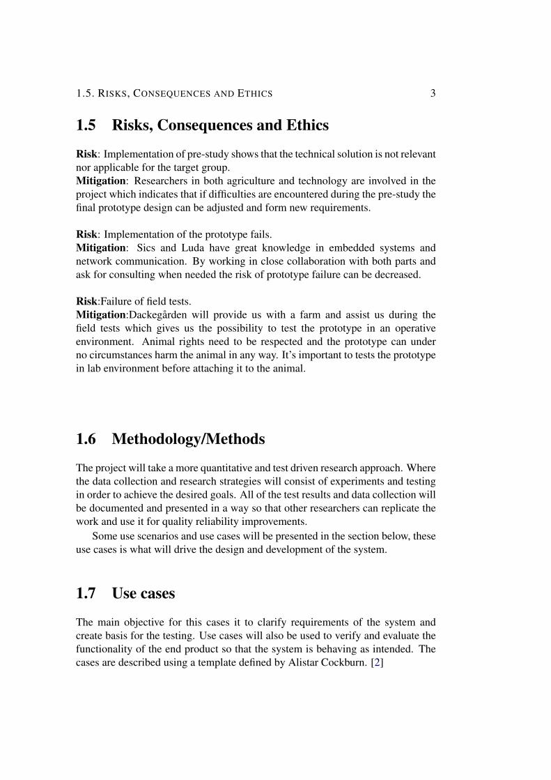
Risk: Implementation of pre-study shows that the technical solution is not relevantnor applicable for the target group.Mitigation: Researchers in both agriculture and technology are involved in theproject which indicates that if difficulties are encountered during the pre-study thefinal prototype design can be adjusted and form new requirements.

Risk: Implementation of the prototype fails.Mitigation: Sics and Luda have great knowledge in embedded systems andnetwork communication. By working in close collaboration with both parts andask for consulting when needed the risk of prototype failure can be decreased.

Risk:Failure of field tests.Mitigation:Dackegarden will provide us with a farm and assist us during thefield tests which gives us the possibility to test the prototype in an operativeenvironment. Animal rights need to be respected and the prototype can underno circumstances harm the animal in any way. It’s important to tests the prototypein lab environment before attaching it to the animal.

1.6 Methodology/Methods

The project will take a more quantitative and test driven research approach. Wherethe data collection and research strategies will consist of experiments and testingin order to achieve the desired goals. All of the test results and data collection willbe documented and presented in a way so that other researchers can replicate thework and use it for quality reliability improvements.

Some use scenarios and use cases will be presented in the section below, theseuse cases is what will drive the design and development of the system.

1.7 Use cases

The main objective for this cases it to clarify requirements of the system andcreate basis for the testing. Use cases will also be used to verify and evaluate thefunctionality of the end product so that the system is behaving as intended. Thecases are described using a template defined by Alistar Cockburn. [2]


Table 1.1: Use case 1: InstallationName Installation and initializationDescription All of the hardware is updated with

latest software and initialized withstandard values. The anchor nodeplacement are strategically chosen foroptimal coverage.

Primary Actor DeveloperPrecondition NoneMinimal guarantees The hardware is delivered and

installed with initial softwareSuccess guarantees The hardware if well prepared and

ready for of the shelf deployment andno additional configuration isrequired

Trigger User orders a monitoring system

Table 1.2: Use case 2: ConfigurationName System ConfigurationDescription The system is customized for the userPrimary Actor Developer and UserPreconditions The installation needed additional

configurationMinimal guarantees The system is configured based on

the shape and size of the pasture landand cattle size

Success guarantees All of the nodes are configurablewirelessly and do need to be detachedfrom collars for further adjustments

Trigger Of the shelf deployment not possibleand need additional configuration

1.7. USE CASES 5

Table 1.3: Use case 3: PresentationName Data PresentationDescription Collected data is presented for the

userPrimary Actor Front end systemPreconditions Cloud platform has accessible and

readable dataMinimal guarantees Cloud data is presented as list of

entry’s gathered form the clouddatabase. User can define the timespan and excursively choose which ofnodes to be presented

Sucess guarantees Data presented in a informativemanner with graphics, illustrationsand animations to make it easier frothe user to see movement patterns andprogression of sensor values.

Trigger User visits an web-applications tocheck the status of each animal in thefarm


Table 1.4: Use case 4: Data collectionName Data CollectionDescription Sensor data is collected from each

node and propagatedopportunistically through the sensornetwork to the cloud platform

Primary Actor SystemPreconditions System installed and customizedMinimal guarantees Any data stream that reaches the

cloud platform each time a nodepasses the gateway node(waterstation)

Success guarantees All of the following data streams areproperly read and stored on each node

1. Encounter data - Record everyinteraction between twoanimals and store it with atime-stamp.

2. Separation log - Record howmany times animals beenseparated and for how long.

3. Sensor readings - Collectambient sensor data

Trigger System deployed by user

1.8 Usage scenarioThis section will describe a typical user scenario of the end system, how a thesystem can be installed, used and interpreted.

Desire is a agriculturist who mends 170 cows and 40 of these cows are aboutto be released into the pasture land. This time a new system is about to be deployedthat will help Desire to monitor her cows in the pasture land.

Every cow has been equipped with a collar with a micro controller on it andsome anchor nodes has been placed out in the grazing area. A gateway nodewith 3G-connectivity need to be placed in a strategic place where cows pass byregularly, preferably a water source where cows drink.

The cows need to be checked upon and counted once or twice per day. Desire

1.8. USAGE SCENARIO 7

would usually start her quad bike, travel to the pasture land and walk in toughterrain in order to complete the inspection. However with the new monitoringsystem she would simply need to open a web-page and receive information aboutevery cow. She is able able to see it’s history log saying which other cows it hasbeen close to and which areas of the pasture land it has passed by at what time

Chapter 2

Technical Background

This chapter introduces the relevant concepts and technologies that can be used todevelop the prototype. Former researches done in related areas are summarized.The chapter also presents and compares several hardware platforms together withcommunication protocols. The goal of this chapter is to investigate optimalcomponents and communication technologies for the prototype based on: powerconsumption, computation performance, price and sensor compatibility.

9

10 CHAPTER 2. TECHNICAL BACKGROUND

2.1 A monitoring systemA typical monitoring system would consist of measuring equipment or sensorsthat collect data about the object that is being monitored. Data that is beingcollected by the sensors needs to be processed and sent to a central databasewhere it is compiled and presented to the observer. An operating system is neededto schedule process of and define communication protocols of the hardwareplatform.

Figure 2.1: Monitoring system

2.2 WSN - Wireless Sensor NetworkA wireless sensor network consists of small sensor nodes communicating amongthemselves using radio signals. Nodes are equipped with different sensorswith an objective of monitoring the physical or environmental conditions ofthe surrounding. Sensor nodes are essentially small computers with basicfunctionality consisting of:

• Processing unit

• Memory

• Power source

• Radio communication module

• Sensors

2.3. COMMUNICATION STACK 11

The processing units main task is to process locally sensed information and storeor forward it to other nodes. Keeping the processing unit in sleep mode for aslong as possible is crucial from a power consumption point of view. Memoryis used to store both the data from sensors and program that is running on thenode. The sensor nodes are meant to be deployed in remote regions where poweroutlets are not available or applicable. WSN nodes are therefore usually equippedwith rechargeable batteries or solar cells depending on the usage. Sensorscomes in different shapes and types capable of monitoring a wide variety ofconditions where most common sensing parameters are temperature, humidity,light, pressure, acceleration and soil moisture[3].

2.3 Communication stack

2.3.1 OSI model - Open System Interaction modelThis section will introduce the basic concepts of the OSI model and point out mainlayers that this research will encounter.

The OSI model is an model that characterizes and standardizes the communicationfunctions by dividing it into seven different abstraction layers. Each layerimplements it’s own functionality and protocols independent of underlyinglayers[4]. Data that is created by an application will start in the top layer andthen propagate down through every abstraction layers utilizing the protocols eachlayer has to offer. The two layers of most interest for this project is Data link layerand the Network layer.

# Layer7 Application6 Presentation5 Session4 Transport3 Network2 Data link1 Physical

Table 2.1: The OSI Model

2.3.1.1 Data link layer

Data link layer provides support for data transmission between two adjacent nodes- a link between to directly connected nodes. It detects and possibly corrects


errors that may occur in the physical layer. The data link layer is responsiblefor establishing a protocol that will open and close a connection between twophysically connected devices. The flow control on each link is also decided bythe Data link layer[4]. Media Access Control (MAC) and Logical Link Control(LLC) are the two sub-layers to data link layer. These two sub-layers have aninternal hierarchy, where LLC is n top of MAC. LLC provides data link controland addressing while MAC controls which of the devices in the network that mayaccess the medium and who has the permission to transmit/receive. Carrier sensemultiple access with collision avoidance (CSMA/CA) is an protocol that onlyallows transmits when the channel is sensed to be in the idle state . Other examplesof protocols that operates in the Data link layer are HDLC, ARP and PPP [5].

2.3.1.2 Network layer

Network Layer is arguably considered one of the most complex layers that hasa main responsibility of providing a host to host communication service. Thisbasically means to move a packet from a sending host to a receiving host thoroughmultiple hops. The service can be divided into two key network-layer functions,forwarding and routing. When a package arrives at a router’s input link, therouter needs to forward the package to the appropriate output link based on theimplemented algorithm on the router. Routing - the network layer must determinethe route or path taken by packets as they flow through the network. The pathis decided by the routing algorithms. RIP, OSPF and BGP are some of the mostcommon routing algorithms in the Internet network.

The network layer complexity can vary depending on the size and architectureof the network. The network service model determines the characteristics of theservices the network has to offer. Some examples of such services may be:

• Guaranteed delivery

• Guaranteed delivery with bounded delay

• In-order packet delivery

• Bandwidth guarantee

The choice of the network architecture should be based on what kind of servicesare needed to meet the requirements of the whole system. For this specific projectit was preferable to implement a more opportunistic delay tolerant system whereservices such as package ordering and guaranteed delivery with bounded delayare not of big significance[6].


2.3.2 IEEE 802.15.4

The IEE 802.15.4 is an standard that specifies the physical layer and media accesscontrol. It was designed in 2003 by the IEE 802.15 working group to addressthe need for low cost, low power wireless standard optimized for monitoringand control applications. The main differences to other wireless IEEE-standardsis it’s fast power-on latency and support of mesh-networking. The 802.15.4standard has became an strong alternative for for low rate wireless solutionswithin the IoT domain. Communication protocol stacks on higher levels such asZigBee, 6LoWPAN and WirelessHART are based on this IEE standard [7]. IEE802.15.4 uses an carrier sense multiple access with collision avoidance (CSMA-CA) method to access the physical medium. The standard also supports optionalmessage acknowledgment to ensure package delivery, energy detection to pickchannels and link quality readings to determine the signal strength. All of thesefeatures contribute to a more reliable data delivery even in environments with highinterference levels[8].

2.3.3 MAC Layer in WSN

In an WSN the main medium used in the network is the radio frequency modulewhich is also the biggest energy consumer of an wireless node. Consequentlythe MAC protocol has additional important functionality to fulfill in an wirelessnetwork. Controlling the radio unit is an crucial part when managing the powerconsumption of any unit using wireless communication.

The MAC protocol is mainly responsible for the power consumption in WSNThe media that is accessed in an WSN is the Radio Frequency (RF) module. Theradio interface is usually the main energy consumer in an typical IoT device andthe most common way of reducing energy consumption is to turn off the RFmodule when it’s not used. This however leads to synchronization challengesbetween the devices in the network. Each node need to know when to expect newdata to be transmitted from it’s neighbors before turning on the RF module. Thetime percentage each node has its RF module turned is called duty cycle. Withproper configuration of the radio duty cycling (RDC) that fits the system designthe energy consumed by the network can be reduced.

2.3.3.1 ContikiMAC

ContikiMAC is an radio duty cycling protocol implemented in the Contiki OSversions 2.5 and above. The mechanism behind the protocol is based on powerefficient wake-up system with a set of timing constraints that allows nodes to turnoff their transceivers devices off when not used.


The most fundamental principles behind the RDC protocols is described inthe figures below. Figure 2.2 illustrates how the receiver nodes sleep most of theirtime and only turned on periodically to check weather there is any activity onthe radio channel. If radio activity is detected by looking at the Radio ReceivedSignal Strength (RSSI) the receiver will stay awake until the next package isdelivered. The sender however will keep sending the same package until the linklayer acknowledgment is received. Figure 2.3 illustrates how the sender behaveswhen an acknowledgment is received.

Figure 2.2: Broadcast transmissions are sent with each packets being resent forthe whole wake-up period of the receiver.

Figure 2.3: Package is received send ack to sender and stop resending

The mechanisms behind the ContikiMAC are build upon earlier RDC-protocols such as B-MAC, X-MAC and Box-MAC using similar wake-up procedure.ContikiMAC was designed with the goal of being easy to understand andimplement without using any additional signaling messages or headers. A moredetailed evaluation of Contiki MACs performance and power consumption can be


found can be found in Adam Dunkles artice The contikimac radio duty cyclingprotocol [9].

2.3.4 Opportunistic NetworksOpportunistic network is considered as an subclass of Delay-Tolerant Network(DNT) where the nodes lack continuous stable connectivity. The link performancebetween an end-to-end path in such network will either have long delays ornot be stable enough for conventional protocols that depend heavily on quickacknowledgment replies[10].

In opportunistic networks nodes will either move out of connectivity range,power down to conserve energy or links may be disrupted or shut down periodically.Infrequent and sporadic connectivity between nodes will lead to network partitions.In order to still be able to send messages from one point to another despite theconnectivity issues there are some functionalities that need to be utilized. Data tobe delivered to its final destination can be stored locally on a intermediate nodeuntil an possible path is available. This will require forwarding and storage abilityof bypassing data from each node in the network. The solution presented aboveonly addresses the issue with complicated applicability of acknowledgment basedprotocols, the delay between end-to-end nodes will still remain the same, thusopportunistic network architecture is only applicable in delay-tolerant systems[11].

2.3.5 ZigBeeThe ZigBee is a standard that defines a set of communication protocols for low-data-rate short range wireless networking. The standard builds on IEE standards802.15.4 which defines the physical and MAC layers. On top of this the ZigBeeprotocol defines application and security layer specifications enabling wirelesscommunication between platforms developed by different manufacturers.TheZigBee wireless devices operates well in harsh radio environments using the858MHz,915MHz and 2,4GHz frequency bands.

The maximum data rate that the ZigBee can reach is roughly 250K bits persecond. ZigBee is not focusing high transfer data rates instead it’s targeted toachieve low cost and long battery life. As a result a ZigBee based devicesare capable of being operational for several years before their batteries needreplacement. This is achieved by letting devices utilize duty cycles by going intosleep mode where power usage is relay low. The duty cycle is a ratio betweenactive time and and time spent in sleep mode. For example if a device wakes upevery minute and stays active for 60 ms the duty cycle would be 60/60000 = 0,001or 0,1%. The power savings of the device is obtained by utilizing the duty cycles


in applications. In most ZigBee based applications the duty cycle is less than 1%to ensure long battery life[7].

Main characteristics:

• Low power usage

• Supports a wide range of different network topologies,including point-to-point, peer to peer and mesh network.

• Highly reliable and secure

• Cost effective

• Scalable and easy deployment

• 250 kbps data rate

2.3.6 6LoWPAN6LoWPAN -IPv6 over Low-power Wireless Personal Area Networks is as ZigBeealso a set of communications protocols defined by IETF(Internet Engineering TaskForce). The 6LoWPAN stack can in addition to the IEE 802.15.4 run on any IP-based physical links such as WiFi and Ethernet[3]. In comparison to ZigBee the6LoWPAN offers better interoperability with other devices in the IP-network dueit’s efficient use of IPv6. In an 6LoWPAN every unit has its own IPv6 address andcan communicate with any other device connected to the IP-network. While theZigBee network requires a translation gateway or proxies to bridge each device tothe IP-network[12].

2.3.7 RimeRime is an lightweight layered communication stack for sensor networks. Itwas developed by Adam Dunkles with a main purpose of simplifying theimplementation of sensor network protocols and reduce the code footprint byupholding code reusage. The main difference between Rime and other modularprotocols is that rime has a strict layering structure where only the lowest layerand application layer can be replaced[13]. Rime consists of strict layers illustratedin figure 2.4 where each layer is designed to be extremely simple both in termsof interface and implementation. Each layer is thin and only focuses on a specifictask if additional functionality is added code from previous layers is reused.The lowest layer is an anonymous best-effort broadcast that simply broadcastsmessages on a channel without any identification, next layer reuses that codestructure and only adds a header to the broadcast message. The stubborn layerwill keep sending same messages until the upper layer tells it to stop. In the

2.4. CONTIKI - OPERATING SYSTEM FOR IOT 17

Figure 2.4: Rime layers

next layer reliable transmission is achieved by adding additional headers to themessage, sequence number and acknowledgment.

2.4 Contiki - Operating system for IoT

Contiki is an open source operating system specially customized to run Internetof Things applications. It low-power communication by connecting low-powermicro-controllers to the internet using the IPv6 and IPv4 standards along with themost recent low-power wireless standards:ZigBee, 6LoWPAN,RPL, CoAP.

Contiki applications are written i standard C and the OS comes with Coojasimulator. The simulator allows networks to be emulated before uploaded into thehardware. Whole development environment can be set up in a single download.

The OS is designed to run on tiny systems having only few kilobytes ofmemory available by implementing highly memory efficient allocation methods.This makes it possible for the Contiki OS to be used in a wide range of hardwareplatforms[14]. There are however a set of platforms that are more popular and aretagged as primary Contiki platforms.

2.5 Hardware platforms for WSN

This section will present a selection of different hardware platforms with wirelessconnectivity. Each platform is examined based on what functionality it has tooffer and at what cost.


2.5.1 ArduinoArduino is an open source hardware and software platform. It was introduced in2005 and was designed with the goal of making the hardware and software easyto use and available to the widest audience possible. The Arduino platform hasan growing community of contributors and a lot of information and tutorials canbe found on their website to help people getting started with their development.Arduino also provides a development environment called Arduino IDE which isbasically a text editor with limited set of functions designed to support compilationand loading of sketches. The IDE is supported on Linux, Mac and Windowscomputers. [15]

There are several Arduino board models available for purchase.Some ofthem are equipped with more powerful processors that can be compared withRaspberry Pi units while others are single purpose processors configured forspecial applications.The variety of different models is big but they all follow abasic layout where every board consists of a USB connection, a power connectorand a standardized set of pins for shield attachments. Shields are modular circuitboards that can add extra functionality to the platform.For instance wirelesscommunications modules such as XBee, Bluetooth and WiFi can be added toArduino platforms using shields.

2.5.2 XbeeThe Xbee is a RF-module developed by Digi that provides embedded solutionsfor wireless endpoint connectivity for different devices. These modules uses theIEEE 802.15.4 networking protocol based on the ZigBee standard.

There are different types of Xbee modules mainly divided in regular and proversions. The regular module is more energy efficient and cheaper compared tothe pro model. It uses the 2.4GHz frequency and has a range limit up to 300m inline of sight. Xbee Pro versions uses the 900MHz frequency which extends therange of the communication and increases object penetration.

Xbee modules are highly compatible with many different hardware platformsand XBee shields makes it easy to add wireless communication to Arduino andRaspberry Pi based projects.

Developer kit XKP9-DMB0 consisting of items below will cost around330USD. Same kit with the cheaper module costs 100USD[16].

• 3x Programmable XBee-PRO 900HP modules

• 3x XBee USB interface board

• Debugger

2.5. HARDWARE PLATFORMS FOR WSN 19

• 2x USB Cables

• Antennas and Accessories

2.5.3 Raspberry PIThe Raspberry Pie is a credit sized single-board computer. It was developed in theUK with the intention to teach the basics of computer science in schools. Todaythe board is widely used around the world and in June 2015 about five to sixmillion Raspberry Pie units has been sold[17].

The latest Raspberry Pi 2 unit has uses an Broadcom BCM2835 SoC modelthat includes: CPU,GPU,DSP,SDRAM and one USB port. The CPU is an900Mhz quad-core Arm processor which is similar chip that is used in oldergeneration of smartphones.The Raspberry platform primarily runs with Linux-kernel based operating systems such as Arch Linux ARM, Raspbian, and RISCOS.

The price of a Raspberry pie unit varies between 20-35 USD depending onthe model.Unfortunately the Raspberry Pie models does not provide any built- inwireless communication and will require an external adapter which will increasethe cost.

Table 2.2: Raspberry pie specificationRaspberry Pi2 Model B Connections900MHz quad-core ARM Cortex-7 17 GPOI pinsGPU with 1080p H.264/MPEG-4 encoding USB2.0 port1GB SDRAM memory shared with GPU HDMI Video Output15-pin MIPI camera interface 10/100Mbit/s EthernetMicroSDHC slot 3,5mm Audio outputPowered with 5V via Micro USB Micro USB port for programming

2.5.4 Texas Instruments SensorTagTexas Instrument offers a sensor tag platform that powers the IoT development.The platform supports several wireless low energy protocols such as,BluetoothSmart, 6LoWPAN and ZigBee. The battery life of a platform running low energyprotocols is estimated to one year with a 1 second report interval.

The SensorTag is running with the CC2650 wireless MCU and comes withsome built-in sensors [18]:


• 9-axis Motion Sensor MPU-950

• Infrared and Ambient Temperature Sensor

• Humidity Sensor

• Barometric Pressure Sensor

SensorTag has a total of 670KB of memory where is 158KB comes from thecc2560 MCU and the remaining 512KB come from the serial flash memory chipattached to the SensorTag [19]. On top of everything the platform comes with anIOs and Android apps where the sensor data can be presented and controlled witha user interface.The price of one unit is roughly 30USD.

2.5.5 PinoccioPinoccio is an open source hardware and software platform with built in 2.4GHzradio communication module using the 802.15.4 IEEE standard(same as theZigBee). It has an on-board temperature sensor and a battery with and rechargingcircuit.

The Pinoccio platform is Arduino compatible and allows the usage of ArduinoIDE together with most of the packages provided for Arduino development.The platform seems to fit very well for prototype development because of it’scomplete package, delivering low-energy wireless communication,built-in batteryand arduino compatibility. The price for one unit is roughly 50USD while a unitthat supports WiFi costs 120 USD

Table 2.3: Pinoccio specification[1]Microcontroller(Atmel ATmega256RFR2) ConnectionsBuilt-in radio for mesh networking 17 digital I/O pins, including four with PWM16MHz MCU 8 analog input pins256k Flash 2 hardware UART serial ports32k SRAM Hardware SPI port8k EEPROM Dedicated I2C port1.8 - 3.3 volt power Micro USB port for charging and programming

2.6. RELATED WORK 21

2.6 Related work

2.6.1 ZebraNetZebraNet is a wireless sensor network project made by graduates and professorsat Princeton university in collaboration with researchers at Mpala Research centerin Kenya. The goal of the ZebraNet was to develop a system that gathers GPSposition samples from zebras over a wide range(100-1000 square kilometers) ofopen lands. The data is then collected and presented to researchers so that theycan learn more about movement patterns, especially during long-term migration.

The study focuses on smart ways to solve wireless communication challengeswhile maintaining low power usage. The resulting collar design uses both longrange and short range radio units where the short range device focuses on errorcorrection and data packaging. The long range radio device is necessary whencommunicating with base station during data collection. Since zebras has a hugegrazing area GPS is used to track the animals and data collection has to doneactively by researches by either bus or flying drones[20].

2.6.2 Seal-2-SealSeal-2-seal research focuses on application of opportunistic networking techniquesto wildlife monitoring. The paper presents a solution based on a protocol whereevery node is able to log contact with other nodes and then disseminate that datafurther to sink nodes using intermittently connected network. The protocol utilizesa novel mechanism that creates efficient data summaries that reduces the amountof data that need to be disseminated by every node.

The Seal 2 Seal protocol [21] is based on two phases, contact detection, anddissemination. During the contact detection nodes periodically listens to signalsfrom other nodes within the transmission range. If a signal is detected the eventis logged as an new contact. Dissemination phase is initiated when new contact islogged and neighboring nodes start to exchange information.

The performance of the protocol is evaluated using Contiki operating systemand Cooja emulator [14].

Chapter 3

System Design

This chapter will describe the architecture of the experimental desgin of a systemmonitoring of cows grazing over pasture lands. It will give a detailed descriptionof the underlying platforms as well as the technology behind the design. Thearchitecture will be explained with a top down approach. Starting out with outerabstract components and then moving down to into more technical segments.

The design goals and decisions were mainly driven by the use cases mentionedin chapter 1.

Figure 3.1: System overview

23

24 CHAPTER 3. SYSTEM DESIGN

3.1 System architecture overviewThe system is divided in three main parts

1. Core WSN - Network of wirelessly connected nodes using opportunisticcommunication.

2. Back-end - Cloud platform for storing and analyzing the data generated bythe WSN.

3. Front-end - Web Page requesting data from the cloud platform and presentsit to the end user.

3.1.1 Core WSNThe core WSN network consists of mobile devices attached to animals, anchornodes placed in the pasture land and a main sink with internet connectivity placednear a water station. Main responsibility of the WSN network is to collect anddistribute the data that is generated by the animals. Information such as ambientsensor data, latest interaction between animals as well as separation time betweenanimals is the kind of data that is collected by each mobile node.

3.1.2 Back EndThe main sink/base station transfers the data further to the back end systemconsisting of a cloud platform. The cloud platform is responsible for filtering andanalyzing the data. The goal of the analysis is to from the raw data input acquireconnectivity patterns between animals and anchor nodes. The patterns can showanomalies in social interactions and indicate on health related problems.

3.1.3 Front EndFront end is developed by Elena Blad who is an Intern at SICS. Front end is in thiscase a web application designed using HTML, PHP, CSS and JavaScript. The webpage requests the filtered and analyzed data from the cloud system and presentsit to the user. Tee user have the opportunity decide what kind of data is to bepresented by either defining time span of when data was generated or search for aspecific node ID.

3.2. SYSTEM ELEMENTS 25

3.2 System elementsThe system can be broken down further into following elements

1. Mobile node

2. Anchor node

3. Sink node / Base station

4. Cloud platform

5. Web interface

Both the mobile and anchor node types use same hardware and run similarsoftware. The important factors of these nodes is the radio communication andstorage possibilities. The mobile nodes are attached to a collar around the neck ofthe animal preferably on top of the neck. Cows are massive animals and and theirbodies can thus absorb or disturb the radio signals. By having the nodes attachedon top of the neck the interference rate of the signals can be reduced.

The anchor nodes should have the identical functionality as the mobile nodesbut instead of being attached to animals the nodes are placed on fixed locationsin the pasture land. All nodes keep record of interaction with other devices andby knowing when a certain animal had an interaction with an anchor node thelocation of the animal can be deduced.

Based on the use cases and requirements the data acquired by the mobile nodescan be divided in three different types:

1. Ambient sensor data is collected using sensors that come with thehardware device. It should however be possible to add external sensorsand connect them to the mobile node device. Temperature sensor andaccelerometer are common sensors that can be used in the experimentalprototype.

2. Encounter Data - As soon as two nodes get in communication range alog about the interaction is created and stored in the local memory. Entriesin data log are created only once for one unique interaction, meaning iftwo nodes meet more than one time only the latest encounter will be loggedoverwriting the previous encounter time-stamp. The local data is also sharedamong all other nearby nodes in the network. In this way the data isdisseminated through the network to the main sink. This allows the mainsink to retrieve data from animals that do not have any direct contact withthe main sink node.

26 CHAPTER 3. SYSTEM DESIGN

3. Separation Data is created when two nodes been apart from each other fora predefined period of time. The data consists of two node IDs and twotime-stamps. The first time-stamp tells when the nodes were separated andthe second time-stamp when they met again.

Sink node is also similar to both mobile node and anchor with a maindifference having a wired connection to the base stations. The sink listens andreceives the data floating int the WSN in same way as the mobile nodes but insteadof sending the data further wirelessly it pushes the data to the base station usingserial communication to. Sink acts as an gateway node being the only point wherethe data can leave the WSN.

The base station should be a more powerful device than the nodes in WSN andsince it will remain stationary near a water station it can have better power supply.The data it receives from the sink node need to be passed further to the cloudplatform via Cellular network. Cellular network connection can be establishedusing a 3g-dongle.

3.3 Choice of technology

3.3.1 Texas Instrument Sensor Tag with ContikiAll nodes in the WSN runs on the Texas instrument sensorTag using the Contikioperating system. There is an active community that continues to develop Contiki.The light weight and flexible Operating system was developed to support the WSNdevelopment. It offers great tools and protocols for a wide range of IoT deviceswith sensorTag being one of them. Communication is a fundamental concept inthis project and Contiki provides communication protocol implementations fromthe application layer down to the physical layer.

The choice behind using sensorTag as the main hardware unit is based on itbeing an primary Contiki platform. The sensorTag platform is actively supportedand included in the current Contiki code tree. The sensorTag also comes fora reasonable price considering it being equipped with 6 different sensors andsupporting IEE 802.14.5, ZigBee and 6LoWPAN.

3.3.2 Communication stack protocolThe table below shows a comparison of some protocols mentioned in chapter2.2. All protocols can operate in the same frequency band(2.4GHz) and have acommunication range between 10-75 meters.

3.3. CHOICE OF TECHNOLOGY 27

Table 3.1: Communication stack comparisonFeature IEE 802.15.4

Rime6loWPAN ZigBee

Possible networktopologies

Star Tree, Mesh Mesh

Over the airprogramming

No No Yes

IPv6 compatible No Yes NoMaximal numberof nodes

Implementationdependent

64000 64000 nodes

Preferred field ofapplication

Point to pointconnections

WPAN with IPconnectivity

HomeautomationWSN

Taking a look on the ZigBee stack that looks very promising offering usefulfeatures. ZigBee was designed specifically to achieve high standards in bothpower consumption and scalability. Despite the perks that ZigBee has to offerthe system in this project will be using the Rime communication stack on top ofthe IEE 802.15.4 standard. Reasoning behind this decision is based on ZigBeebeing proprietary, controlled by the ZigBee alliance group. ZigBee alliance offersseveral applications and network standards. However the source code for thestandards can not be viewed or edited without being a ZigBee alliance member.These restrictions would make it hard to customize the standard to fit the desiredfunctionality of the system. Rime does not offer same amount of features as theZigBee stack but allows more flexibility in the implementation.

3.3.3 Raspberry pie as the base stationThe base station that forwards the data acquired by the WSN needs to beslightly more powerful than the sensorTags and does not have the same powerconsumption restrictions. It needs to be compatible with a 3G-dongle and be ableto process and pack the data to format that is readable by the cloud platform. Thecriteria above can be met by using a Raspberry Pie running the Raspbian OS.The choice here is based on the great amount of documentation available for theplatform as well as some previous development experience.

Chapter 4

Implementation

This chapter will describe how the technologies and the equipment were used todevelop the experimental prototype of the system. Additionally the implementationof data structures and data dissemination will be explained in detail.

4.1 System overview

Figure 4.1: System overview

29

30 CHAPTER 4. IMPLEMENTATION

4.1.1 Contiki build systemThe Contiki build system is based on configuring project header files or customizingMakefiles. In the project header file the developer is able to specify the networkrelated parameters such as network stack, RDC check rates or Radio frequencies.The WSN nodes in this project used the NETSACK with Rime configurationand RDC check rate of 16 which was an default value that. Down below is anextraction of configurations in the header files used during implementation of thesystem.

CONTIKI_WITH_RIME = 1define NETSTACK_CONF_RDC contikimac_driverdefine NETSTACK_CONF_RDC_CHANNEL_CHECK_RATE 16

The Makefile specifies where the Contiki source code resides in the native systemand includes platform specific libraries defined by the BOARD parameter.

make BOARD=sensortag/cc2650

After running the make file an image file is compiled containing the Contiki OSwith the developed program ready to be uploaded to the hardware platform.

4.1.2 Data generation and representationAccording to the system design the system need to collect three types of data.

1. Ambient sensor data

2. Encounter data.

3. Separation data.

Ambient sensor data is acquired by using the Texas instrument library functions.In order to read the values the sensors need to be activated and then initiated withsample rate timer. The register that holds the sensor measurement value is thenread periodically.

Every node in the WSN sends a beacon signal periodically when a beaconis received by other nodes an encounter entry is created and stored in the localmemory of the node. This way of implementing the encounter detection isinspired by the Seal-2-Seal protocol[21] that is mentioned in section 2.5.2. Eachencounter is represented as a struct containing three entries. Node ID, Encounternode ID and a time-stamp. The struct is then added to a linked list calledEncounter list that holds all of the encounters created in the network. The currentimplementation only logs the latest encounter meaning if an encounter occurs

4.1. SYSTEM OVERVIEW 31

more than once only the latest one will be kept in the encounter list with anupdated time-stamp.

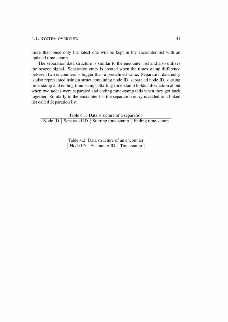
The separation data structure is similar to the encounter list and also utilizesthe beacon signal. Separation entry is created when the times-stamp differencebetween two encounters is bigger than a predefined value. Separation data entryis also represented using a struct containing node ID, separated node ID, startingtime-stamp and ending time-stamp. Starting time-stamp holds information aboutwhen two nodes were separated and ending time-stamp tells when they got backtogether. Similarly to the encounter list the separation entry is added to a linkedlist called Separation list.

Table 4.1: Data structure of a separationNode ID Separated ID Starting time-stamp Ending time-stamp

Table 4.2: Data structure of an encounterNode ID Encounter ID Time-stamp


4.2 Data collection and disseminationEach of the data streams need to be collected and propagated with an opportunisticapproach. One way of doing this as mentioned in section 2.2.4 having each nodehave a copy the data that needs to be disseminated. How the data is disseminatedwill be explained by describing the processes that run on each node. Rime that ismentioned in section 2.2.7 is used for establishing communication and exchangingdata between nodes.

Figure 4.2 illustrates important data structures and processes that are implementedon each node and how the data is flowing when two nodes are within radiocommunication range.

Figure 4.2: Data flow during an encounter

Data structures used in the implementation are following:

• Broadcast beacon - Struct consisting of senders ID a time-stamp

• Unicast message - Same structure as an entry in the encounter list or historylog.

• Neighbor list - List of addresses to current neighbor nodes

• Encounter list - List of encounters between all nodes.

• Separation list - List of all separations between nodes

4.2. DATA COLLECTION AND DISSEMINATION 33

Every node runs 5 processes and implementations of these processes setsthe core functionality of the WSN. The processes are defined and implementedfollowing Contiki guidelines with an event or timer triggered processes.

4.2.1 Send BroadcastThis processes simply sends a a broadcast beacon every t second to every addressin the neighbor list. Sensor values that are read locally from each node are packedand added to the broadcast beacon message.

4.2.2 Receive BroadcastWhen a node receives a broadcast message it parses the data from it and createsnew entries to the neighbor list and encounter list. Receiving a broadcast messagecorresponds to an encounter between nodes and a new encounter entry can only becreated by this process. Each broadcast message comes with the senders physicaladdress which is stored in the neighbor list. If the broadcast is received for thefirst time from the senders node a new entry is created and added to the encounterlist otherwise the old entry is overwritten with new time-stamp and sensor values.

An entry in the local separation list list is also created by this process. Theentry is created based on two conditions. Receiver node already encounteredthe sender before and the time-stamp difference between the first and secondencounter is bigger than a predefined value t.

4.2.3 Send UnicastThe process iterates though the neighbor list and encounter lists and sends wholeencounter list to every neighbor in the neighbor list. When this is done theneighbor list is wiped out, this allows a more dynamic tracking of neighbors wherethe data is only sent to current neighbors. The encounter list is chopped down tosmaller fragments where each entry in the encounter list is packed into a singleunicast message. For example if a node has 10 encounters stored in the encounterlist with two neighbors it would need to in total send 20 unicast messages.

4.2.4 Receive UnicastThis process receives data stream of unicast messages where every message iseither an encounter or an history log entry. If the entry already exists in the localstorage only the time-stamp and sensor value is updated otherwise a new entry isadded to the encounter list.


4.2.5 Sensor readingsThis process activates and reads sensor values from the hardware. Also usedfor troubleshooting and printing current state of each data structure. Time-stampcounter is incremented by this process.

4.3 Optimization and improvementsThis section describes the improvements and optimization during the secondcycle of prototype development. After the first cycle the prototype the nodeswere able to communicate and acquire the data that specified in the minimalrequirements. Through out the second cycle functionality optimization wereadded to the prototype continuously that mainly targeted the resource and powermanagement.

4.3.1 Merging dataInitially the first prototype had a third data structure that needed to be sent acrossthe network holding sensor readings similar to the encounter and separation lists.Improvements could be made by merging the sensor data stream together withthe encounter which eliminated the need of additional data structure and lead toreduced memory usage and lower power consumption due to smaller overhead inmessages. The merged encounter data structure went from having three elementsto seven.

Table 4.3: Merged data structure of an encounterNode A Node B Time-stamp Temp A Temp B Activity A Activity B

4.3.2 Allow easy configurationThe power consumption of each node is mainly dependent on the radio transceiverunit activity. Having the ability to control and influence radio module activityis crucial for power management purposes. Even if most of the controlling ishandled in low level protocols such as RDC and Contiki MAC the applicationrunning on each node can still have a big impact on the power consumption.Broadcast and unicast are the processes that activate the radio unit and bycontrolling how often the processes are allowed to run will directly affect for howlong the radio module can stay in sleep mode. This is however a trade-off betweenpower consumption and functionality of the whole system, having broadcast

4.4. BASE STATION AND SINK NODE 35

processes run less frequently means higher chance of missing an encounter ornodes having to old data. Keeping this in mind during deployment and allow easyconfiguration of how often processes are allowed to use the radio unit will makeit easier to find optimal values that keeps same functionality level and preservespower usage.

4.3.3 Data sent trackingThe first implementation of unicast processes was basically iterating through thecurrent neighbor list and sending data to each of the neighbor nodes. This meantthat if a node only had one neighbor it would keep sending same data to samenode over and over again. Adding a small times-tamp entry to the neighbor structthat keeps track on when last data was sent to that node allows the unicast processto discard the neighbor if the data already been sent to that node recently.

4.4 Base station and sink nodeAs stated before the difference between a sink node and a mobile node i verysmall. The sink node need to have an debugger attached to it so that it can usethe serial output and the send unicast process can be deleted because the sinkdo not need to send the data back to the WSN. The sensor reading process isreplaced with serial print process. The process continuously iterates through thelocal encounter and separation lists and prints its content to the serial output.

The base station in our case an Raspberry pie unit is connected to the sinknode serially and reads the incoming data with a python script. The data is thenparsed, converted into a JSON objects and sent to the cloud over the 3G network.

Figure 4.3: Data flow from WSN to Cloud

Chapter 5

Testing and deployment experience

This chapter describes three different tests that were used during the projectand drove the development forward. The test setup and test scenario will bepresented together with the results from each testing method. The goal of thetests is to assure that the system works as intended and keep improving it until therequirements in the user cases are met

5.1 Cooja simulation testsCooja simulator comes together with the Contiki development environment canfully simulate 11 different hardware platforms[14]. Unfortunately the sensorTagthat is used in this project is not fully supported meaning that the platform specificlibraries such as sensors and buttons can not be simulated properly. The networkrelated modules however such as Rime and RDC and ContikiMAC[9] can still betested by running the simulation for a platform similar to the sensorTag.

5.1.1 Simulator advantagesThe development was test driven where every small functional progress was testedusing the simulation environment, especially during the network related tasks.The simulator is great tool and saved a lot of time. Running the tests directly onthe hardware would complicate a lot of the work. Without the simulator everysmall change in the code would require that the new updated image would haveto be uploaded on every unit. Flashing a single device takes about 2 minutes andtesting some of the data collecting functions would require minimum of 5 sensorTags, meaning that it would take around 10 minutes to update the system or fixa bug. Another big problem that got simplified by using the simulator was thetest based on he wireless connectivity range. A great deal of tests were based on

37

38 CHAPTER 5. TESTING AND DEPLOYMENT EXPERIENCE

having two nodes going out of connectivity range in order to test the generation ofencounter data and separation log. Without the simulator the tests would requireto physically walk away with a node until the signal was lost and then walk backagain which would also lead to a very time consuming testing method.

Cooja simulator comes with an informative and intuitive graphical userinterface. When a node is uploaded to the environment it appears as an moteobject in the graphical grid. When clicking on a mote the connectivity range isvisible as bigger circle around the mote. The motes are also easy movable out ofeach others connectivity range. Updates of code versions can simply uploaded toevery mote in the grid by clicking the reload button.

5.1.2 Simulation test setupAs previously mentioned a great deal of functionality was tested using thesimulation tool, this section will describe one specific test that was done in laterstage of development. Starting off with the test case setup and then moving on tothe test results that will be presented using screenshots and system print outs.

Test case for the simulation tool consists of 7 motes in total: 3 anchor motes,1 sink mote and 3 mobile motes. To simplify the testing scenario lets divide thetest in four events.

1. Event 1- Initial state, all of he mobile motes start out within a range of thesink node.

2. Event 2- Move to anchor node, mobile motes move out of the sink node todifferent anchor nodes

3. Event 3- Gather up, all mobile motes gather up at one anchor

4. Event 4- One mote goes back to sink mote.

The deployment of this testing scenario will cover the minimal requirementsof the system. The test covers the events of two or more node encounterswhich should generate data in the encounter list and nodes benign separated fora while and then getting back together should create data in the separation log.Unfortunately sensor readings can’t be tested with this test since Cooja not fullysupporting the sensorTag platform. The simulation platform used in this case wasan Tmote Sky mote which uses similar radio module as the sensorTag.

5.1.3 Simulation resultsThe results from the simulation for each of the event will be presented with ascreenshot of showing the placement of each mote together with a system print

5.1. COOJA SIMULATION TESTS 39

out of from the sink node. The print out of the sink node is the data that would besent further to the base station (Raspberry pie).

Table 5.1: Definition of simulated node typesSink Node 7Anchor Nodes 1 2 3Mobile Nodes 4 5 6

5.1.3.1 Event 1

Initial state, mobile nodes are started within the communication range of the sinknode. Event 1 is ongoing between time-stamp 0 and 50.

Figure 5.1: Event 1 - simulated

ENCOUNTERS 0: COW ID 7.0 Encounter 5.0, with timestamp48ENCOUNTERS 1: COW ID 7.0 Encounter 6.0, with timestamp46ENCOUNTERS 2: COW ID 7.0 Encounter 4.0, with timestamp46ENCOUNTERS 3: COW ID 5.0 Encounter 6.0, with timestamp39ENCOUNTERS 4: COW ID 5.0 Encounter 4.0, with timestamp39ENCOUNTERS 5: COW ID 4.0 Encounter 6.0, with timestamp37Current Timestamp: 48


5.1.3.2 Event 2

Mobile nodes are spread to different anchor nodes. The sink node is not receivingany new data and only the current time-stamp of the system is printed. Event 2 isongoing between time-stamp 50 and 100.


Current Timestamp: 100

5.1.3.3 Event 3

All mobile nodes are gathered at anchor node 3, the sink node still does not haveany new data to print. Event 3 is on ongoing between time-stamp 100 and 170

Current Timestamp: 170

5.1. COOJA SIMULATION TESTS 41


5.1.3.4 Event 4

Mobile node 5 is moved back to sink node and sends the data it has collectedbetween event 1 and 3 to the sink.



Encounter list:ENCOUNTERS 0: COW ID 7.0 Encounter 5.0, with timestamp235ENCOUNTERS 1: COW ID 7.0 Encounter 6.0, with timestamp46ENCOUNTERS 2: COW ID 7.0 Encounter 4.0, with timestamp46ENCOUNTERS 3: COW ID 5.0 Encounter 6.0, with timestamp39ENCOUNTERS 4: COW ID 5.0 Encounter 4.0, with timestamp39ENCOUNTERS 5: COW ID 4.0 Encounter 6.0, with timestamp37ENCOUNTERS 6: COW ID 5.0 Encounter 3.0, with timestamp169ENCOUNTERS 7: COW ID 6.0 Encounter 1.0, with timestamp106ENCOUNTERS 8: COW ID 4.0 Encounter 2.0, with timestamp109ENCOUNTERS 9: COW ID 3.0 Encounter 4.0, with timestamp162ENCOUNTERS 10: COW ID 6.0 Encounter 3.0, with timestamp163History log:COW ID 7.0 was separated from 5.0, during timestamps:48-170COW ID 5.0 was separated from 4.0, during timestamps:46-109COW ID 5.0 was separated from 6.0, during timestamps:48-110COW ID 6.0 was separated from 4.0, during timestamps:46-109Current Timestamp: 200

5.2 Indoor testThe indoor test was carried out inside the SICS building to assure a test that coverthe whole system functionality. Unlike the simulation test the sensors and the basestation together with cloud platform could be tested properly.

5.2.1 SetupTo make it easier to interpret and compare test results the indoor test used the samefour event based test case as in the simulations test. There are however somedifferences on how the data represented, each encounter post has 5 additionalelements in its structure. Node ID and Encounter ID together with a time-stamphas the same structure but in the indoor test additional data could be acquired. Asmentioned in section 4.3.1 the ambient sensor data is merged with encounter data.

Table 5.2: Merged encounter data structureNode A Node B Time-stamp TempA TempB ActivityA ActivityB

The activity sensor was tuned in a way where values between 80-130 meant anode being still and not moving, deviation from these values means higher activity

5.2. INDOOR TEST 43

and 0 means a reading error from the sensor . To catch precise activity movementrequired higher sample rate which could not be applicable together with otherprocesses, more about this issue will be discussed in the evaluation chapter.

Same amount of nodes were used in the indoor test as in the simulation but thenodes are named after their rime addresses.

Table 5.3: Definition of indoor tested nodesSink Node 40.131Anchor Nodes 100.1 133.133 213.5Mobile Nodes 203.133 227.128 56.128

How the anchor nodes and the sink node were placed in the building iillustrated in the figure 5.5.

Figure 5.5: Indoor test node placement

5.2.2 DeploymentThe system print out from the sink node in this test was changed to differentformat to make it easier for the base station to parse it and transform it into JSON


format. Data from the Encounter list is labeled as DATA and Separation list datais labeled as HISTORY. Each entry in respective lists are separated by semicolon.

The test was deployed in similar manner as in the simulation, starting of themobile nodes within the range of the sink node. Start the anchor nodes in differentlocations show sown in figure 5.5. When the anchor nodes were setup the testcontinued with moving the mobile nodes according to the events described 5.1.2.

5.2.3 Results5.2.3.1 Event 1

The mobile node are uploaded with the new code and started close to the sinknode. This action generated following data that was sent to the base station.

Timestamp 10 -60DATA:40.131; 203.133; 53;30.812;27.62;37;0;65506DATA:227.128; 203.133; 47;26.843;27.187;115;0;65518DATA:40.131; 56.128; 52;30.812;27.00;37;105;65505DATA:40.131; 227.128; 52;30.812;26.843;37;116;65503DATA:203.133; 56.128; 44;27.218;27.125;0;114;65529DATA:227.128; 56.128 45;26.832;27.122;115;114;65512

5.2.3.2 Event 2

All mobile nodes were moved to respective anchor nodes at time-stamp 60-130.No new data for the sink node to print.

203.133 -> 133.13356.128 -> 100.1227.128 -> 213.5

5.2.3.3 Event 3

All mobile nodes moved to the anchor node 100.1. The results from this test maydiffer from the simulations because there was no way to get node 203.133 to 100.1without passing the sink node due to the shape of the building. Time-stamp 130-270.

5.2.3.4 Event 4

Mobile node 227.127 moved back to the sink node at time-stamp 240 to share thedata it has collected. Sink node then prints the updated data it has received.

5.2. INDOOR TEST 45

HISTORY:40.131;227.128;84;238HISTORY:227.128;203.133;77;128HISTORY:203.133;56.128;88;129HISTORY:227.123;56.128;77;128

HISTORY:227.128;100.1;90;129HISTORY:203.133;40.131;87;122

DATA:40.131; 203.133; 53; 30.812;27.62;37; 0; 65506DATA:203.133; 113.133; 30; 0.000; 0.00; 0; 99; 65446DATA:227.128; 40.131; 80;26.593;30.968;118;3;65503DATA:227.128; 203.133; 59; 26.781;27.00;113;0;65509DATA:40.131; 56.128; 89; 30.937;26.500;31;116;65448DATA:40.131; 227.128; 271; 30.593;25.156;95;113;65508DATA:227.128; 113.133; 44; 26.937;24.906;113;98;65447DATA:203.133; 56.128; 64;26.937;26.750;0;105;65503DATA:56.128; 227.128; 64;26.750;26.718;105;117;65515

5.2.4 Verification and data analysisThe test case was created using a controlled and predefined events to ensure thatthe system produces a very specific output that can easily be verified. Additionallysame test case was used in two different testing environments to simplify thecomparison of the test results. Since there are three different types of data thatwas generated the verification can be done separately for each one of the datastreams.

Encounters verification can be done by taking a closer look at what happenedduring event one and four. In the first event when all mobile nodes are deployedclose to the sink and the expected outcome should have six encounters - sinknode encountering with three mobile nodes and three encounters between mobilenodes.

During the fourth event the expected outcome should have five additionalencounters. Three encounters are added when each of the mobile nodes encounterthe anchor nodes and additional two encounters when mobile nodes gather upclose to a single anchor node during the third event. The expected outcomeshould have a total of 11 unique encounters during the fourth event. The table5.4 illustrates a comparison between expected outcome and test results.

Separation data can be verified in a similar way by comparing the resultsacquired during the fourth event with expected outcome. The only time whenmobile nodes are separated happens during event two and three. Mobile nodesseparate from each-other and then gather up again during the thirds event close to


an anchor node. The separation list does not reach the sink node until the fourthevent which also should add one entry to the separation list. The course of eventsshould in total generate 4 entries in the separation log, three between the mobilenode and one when one of the mobile nodes get back to the sink.

Table 5.4: Data verificationExpected outcome Simulation results Indoor test result

Encountersduring event 1

6 6 6

Encountersduring event 4

11 11 12

Separationsduring event 4

4 4 6

Temperaturesensor

25-27C - 25-30C

Activity sensors 80-120 - 0 -120

Deviation in the indoor results were caused due to the shape of the building.One separation log was created between the first third event when node 227.128had to pass additional anchor node 100.1 in the middle of the hallway beforereaching it’s final destination. The second separation log was added during thethird event when node 203.133 had to pass the sink node on the way to the anchornode 100.1.

The time-stamps for both encounter and separation data show that the courseof events uphold the correct order. Separation logs show that three mobile nodeswere separated between time-stamps 80 -130 which corresponds to separation atstart of second event and the meet up at the third event.

Ambient sensors was not the main scope for the test and had a lower prioritynevertheless there seem to bee a small deviation in the temperature values betweenthe sink node and all other nodes. This was caused due to the debugger attachedto the sink node which affected the ambient temperature measurement.

5.3 Field testThe final field test was carried out on farm called Dackegraden. Dackegarden isfarm located in northern Sweden with a total of 450 cows. The farm is ownedand maintained by Hakansson family. Desire Hakansson was our contact personand the host at the farm who helped us to execute the field test. Before our arrivalDesire sent us the map of the grazing land that had an area of 4 hectares so that

5.3. FIELD TEST 47

we could prepare and plan the deployment of the test. Additional sensroTags wereordered for the final test, ending up with a total of 18 sensorTag units.

5.3.1 SetupThe grazing land was empty upon our arrival which allowed us make last minuteconfiguration and setup the anchor nodes. Initially range tests were made in thegrazing environment in order to decide on where to set up the anchor nodes.

Range test result showed that the communication range between two nodescould go up to 30 meters. Based on these results the anchor nodes were placedaccording to the map in the figure below.

Figure 5.6: Node setup during field test

A total of 18 sensorTags were used during the field test: 1 sink node, 6 anchornodes and 11 mobile nodes.

5.3.2 DeploymentThe deployment process started of with encapsulating sensorTags and the Raspberrypie in plastic cases as a water and impact protection. Not all of the 450 cows were


Table 5.5: Definition of field tested nodesSink Node 40.131Anchor Nodes 100.1, 133.133, 213.5, 56.128, 227.128, 148.5Mobile Nodes 203.133, 163.13, 5.3, 207.2, 144.1, 124.113, 191.6, 130.2, 159.2, 108.3, 102.1

participating in the test. A selection of roughly 30 cows were going to be releasedinto the prepared grazing area. 10 of those cows were equipped with sensorTagcollars. The cows were released after the anchor nodes, sink node and base stationwere up and running.

Figure 5.7: Anchor node and base station

Figure 5.8: Mobile nodes on collar

5.3.3 ResultsData acquired during the field test is presented on the website www.majros.rf.gd.Data that reaches the sink node is forwarded to the cloud system via the base

www.majros.rf.gd

5.3. FIELD TEST 49

station. The front end is in this case a website that fetches data from the cloudplatform and presents it for the user. The layout of the website and how the datais presented is illustrated appendix A.

5.3.4 Problems during field testThe results showed that the separation log was not properly disseminated andonly local separation records from the sink node appeared appeared in the cloud.Unfortunately when the error was detected there was not much that could be doneto address the issue. Dismantling every node from each cow could not be doneeasily without having to bring the cows back to the barn.

Range tests were executed before the anchor nodes were placed to avoidhaving a fully connected network. The range tests showed that nodes had a aconnectivity range between 30-40 meters but the test results however showedcontinuous encounters between the sink node an anchor node that was 100 metersaway. The main difference between that specific anchor node compared to otherwas that it was attached to a tree at high altitude which greatly increased thewireless connectivity range.

The system logs time as a counter that periodically increases its vales. Thebase station is then suppose to transition the time-stamps into time in UTC formatknowing at what time system was started. Test results on the front end showedthat translation did not work properly and represented wrong UTC time.

Chapter 6

Evaluation

The developed experimental prototype of the system, will be evaluated based onthe requirements described by the user cases in chapter 1. This chapter will alsodiscuss the scalability, performance and precision of the system.

6.1 Requirements evaluationThis section will reflect back to the user cases presented in chapter one andevaluate them. Initially four user cases were defined to clarify what is to beexpected from the experimental prototype. Use cases are evaluated by lookingon results of the system and discussing how well the requirements are met.

1. Installation ad initialization . Test results from the field test show that theanchor placement is an crucial part during the installation. Line of sightand altitude differences in the environment need to be taken into accountwhich makes it hard to prepare the software for of the shelf deployment.It’s preferable examine and run range tests on the pasture land beforeinstallation.

2. System configuration. Current implementation of allows configuration ofkey parameters but it can not be done wirelessly. Every node has to bedetached from the collars and reprogrammed with a PC that has Contikienvironment.

3. Data collection.The indoor test results show that the system is capable of collecting theencounter data separation log and ambient sensor readings. However duringthe field test when more nodes were added to the system the requirement forthe use cases was not fully met and only parts of data stream were collectedproperly.

51

52 CHAPTER 6. EVALUATION

4. Data presentation. The front end that was developed by Elena Blad internat SICS is currently presenting the data on web based user interface. Wherethe user is able to search for a specific node, sort and filter the data presentedin table format. Data is fetched from the cloud system and presented in astatic table format.

6.2 ScalabilityThis section focus on discussing the scalability of the system. How the system willbehave when the amount of nodes is increased increased in terms of functionalityand performance.

6.2.1 Memory consumptionCurrent implementation of the system requires a certain amount of memory formeach of the nodes in order to store all of the encounter and separation data. Toget a picture on how much memory is required from one node we can start off bylooking on what kind of data types are created when an encounter occurs.

Table 6.1: Encounter data typesRimeAddr

RimeAddr

uint uint uint uint uint uint

NodeA NodeB Time-stamp TempA TempB ActivityA ActivityB RSSI

Table 6.2: Separation data typesRime Addr Rime addr uint uintNode ID Separated ID Starting time-stamp Ending time-stamp

Contiki uses an 16bit system meaning that both the address data type andunsigned integer consumes 16 bits. Which means that one encounter consumes16*8=128bits (16bytes) and a singe separation log 16*4 = 64 bits (8bytes).

6.2.1.1 Encounter scalability

The maximal amount of possible encounters depends on how many nodes aredeployed in the system. Some optimization were made in the implementationto reduce memory consumption by saying that Node A encountering Node B isequivalent to Node B encountering Node A.

6.2. SCALABILITY 53

Example below shows the maximal amount encounters that can be generatedwith four nodes in the system.

Table 6.3: Maximal amount of encountersA B C D

A - 1 1 1B - - 1 1C - - - 1D - - - -

The table above show that if there is four nodes in the system the maximalamount of possible encounters will be six. Using the same table a moregeneral equation that describes the amount of encounters n using x nodes canbe formulated.

n =x2− x

2;x > 1 (6.1)

The amount of memory one encounter post consumes was estimated to be 16bytes and by adding this value to previous equation will give us a new equationthat describes the relation between amount of nodes and memory consumption iny bytes of the encounter data.

y = 16(x2− x

2)→ y = 8(x2− x);x > 1 (6.2)

Figure 6.1: Memory consumption of encounter data

200 400 600 800 1,0000

0.2

0.4

0.6

0.8

1·106

x(Nodes)

Mem

ory(

Byt

es)

The graph illustrates that in a system with 1000 nodes the encounter listswould approximately consume 1MB of memory.


6.2.1.2 Separation log scalability

Separation log compared to the encounter list does not just update its old value inthe memory, every separation is unique and need to be stored separately. Whichmeans that there is theoretically no limit on how much data that can be stored inthe separation list as time progresses. The limit is set during the configurationof the system where the user define how many separations are saved until oldervalues starts to get overwritten. The separation log is implemented as a circularbuffer using a FIFO (first in first out) algorithm where size of the buffer is whatdecides how much of the memory is dedicated to store separations. The memoryconsumption of the separation log is heavily dependent on the configuration of thesystem. Separation time is another configurable value that decides for how longtwo nodes are separated before a log is created. A higher value will generate lesslogs but increase the risk of missing a shorter separation.

How the memory consumption of the separation log behaves when the wholesystem is scaled up is a trade off between precision and memory capacity. Havinga bigger buffer size and will decrease the chance of useful data being overwrittenand shorter separation time gives more precision on detecting shorter separationbut will require more memory from the system.

6.2.2 Network congestionMemory may not be the only issue when discussing the scalability of thesystem. Already during the field test we noticed some of the congestion issueswhere separation data was not disseminating properly. A fundamental partof opportunistic network implementations is to have nodes store and forwardbypassing data to its intermediate nodes. This approach will work well insituations where nodes are evenly spread. However in situations where nodesare clustered within the communication range the protocol will have difficultiesand lead to redundant data being sent to every neighbor and causing congestion. Aviable solution for this issue was presented in section 4.3.3 where a delay is addedbefore data is sent to same node. In a more scalable system the delay time has tobe more like a dynamic value that can sense the congestion and set the delay timeaccordingly.

6.3 Power consumptionThe sensorTag comes uses CR2032 button cell lithium battery with a typicalcapacity of 225mAh. Texas instrument the manufacturer of sensor promisesa battery life up to two years with their stock software based on low energy

6.4. COST EVALUATION 55

bluetooth running on the platform. Unfortunately the current implementation ofthe monitoring system was no way near to reach same battery life time. Bluetoothmay consume less energy but does not meet the connectivity range requirements.

The system is implemented in this project is using the IEEE 802.15.4 wirelessstandard was able to reach a battery life of 3 days. This is not good enough andforcing the farmer to replace the batteries every 3 days would just lead to loosingthe purpose of the whole system making the monitoring easier. A solution forthis wold be to add an external battery pack. Cows are big animals and wouldnot have any bigger problems having some additional weight around their necks.A power bank with a capacity of 2200 mAh 10 times more than the button cellbattery that costs around 10 USD and weights 93g would significantly increasethe performance in terms of battery life.

6.4 Cost evaluationOne of the goals of the system was to find a way to monitor grazing animalswithout using a GPS module due to it’s high cost high power consumption. Evenif the field test results showed that there is still a loot of room for improvementsregarding the position tracking at least the simulation and indoor test show thatthere it is potentially possible to estimate position of nodes using anchor nodes.In the previous chapter the power consumption was discussed and concluded inthat additional power bank need to be added into final cost of of each unit. Inorder to use the power bank a debugger needs to be attached to the sensorTag forits mini USB connectivity. Table below sums up the total cost for each node.

Table 6.4: Component priceComponent Price in USDTI Simplelink cc2650 SensosrTag 30TI CC Debugger 162200 mAh power bank 10

Total price of each node ends up at 56USD. A solution based on GPSpositioning would add roughly 20USD (depending on precision requirement)perunit and wold most likely require a stronger power bank. The cost of debuggercould also be reduced by replacing it with a customized charging socket.


6.5 Sensor precisionAs the project went forward the ambient sensors precision was less prioritized.After consulting with Anders Herlin, researcher at Swedish University of AgriculturalSciences with experience in similar project where technology is used to monitoranimal health and behavior important knowledge was discovered. The temperaturesensor in the sensorTag would not be able to measure useful temperature unlessthe measurements were taken inside the ear. Getting useful physical activitymeasurements that can be analyzed requires high sample rate and data processingwhich limited resources when nodes uses most of its computation power tomaintain the communication stack.

Despite the discovery of lacking usefulness of sensor readings the systemwas still implemented measuring the environment temperature and activity withlow sample rate. This was done to show that if future enhancement were tobe developed the network protocol could support the dissemination of improvedsensor readings.

The activity measurements could reach higher precision by using an externalDSP(Digital Signal Processor). DSP is an specialized microprocessor used tomeasure, filter or compress continuous analog signals with high sample rate.A DSP allows execution of powerful algorithms that can distinguish differentactivity levels with higher precision. To improve the temperature precision anexternal thermometer would have to be added inside the ear of the animal.

Chapter 7

Conclusions

This chapter explains the conclusions obtained throughout the design, development,and evaluation described in this thesis and proposes a number of improvements,extensions, or complements that may be of interest in order to continue this work.

7.1 ConclusionThe main goal of this project was to develop a system that monitors grazinganimals. The thesis focused on investigating a solution that does not involve GPSor GSM modules on every node in order to reduce the cost of the system. Ratherthan examining the possibility of using an opportunistic wireless sensor networkprotocol to determine an estimated position of each animal by analyzing encounterand separation data between each node in the network.

In conclusion the current implementation of the system has a WSN corenetwork that collects and disseminates data within the grazing area. When datareaches a sink node it passes it to a base station that then sends it further to thecloud platform via the cellular network. The data is then fetched from the cloudand presented to the end use on a website.

Proposed system solution was tested and evaluated in 3 different environments(simulations, indoor tests and field test). To come to the conclusion that it ispossible to acquire sensor data and disseminate it opportunistically and determinean approximate position of nodes. The results acquired by the simulation andindoor tests are verified by comparing system outcome with predefined events inreality. Scalability of the system is examined and evaluated based on power andmemory constrains.

57

58 CHAPTER 7. CONCLUSIONS

7.1.1 Insights and suggestions for further workOne of the most important insights to come from this work is to understandthe possibilities and restriction that comes with different communication stacksand hardware platforms currently available at a reasonable price. The systemdeveloped during this thesis is using a hardware platform supported by Contiki OSand Rime communication. However it would be interesting to see a comparisonbetween implementations that uses different communication stack such as ZigBeeor 6LoWPAN running on different platforms.

The sensors readings were initially a vital part of the research, the goal wasto use the sensor data to determine the well being of of animal that is monitoredand alarm the farmer if abnormalities are detected. The sensors that came withthe SensorTag were not precise enough to generate such measurements. Futurework should include external sensors that can measure the temperature from insidethe ear of the animal and have more powerful activity meters that support highersample rates. C

7.2 Future workIn these section we will focus on some of the remaining issues that should beaddressed in future work.

Some problems that were encountered during the field test has not beenaddressed yet.The separation log problem is fixed but not fully tested with largeramount of nodes. The issue with time-stamp transition to UTC time remains asproblem to be solved. As mentioned in previous section the future work shouldinvolve examination of using external sensors for higher precision and more usefulsensor readings.

The current opportunistic network protocol has some room for improvement.Tagging data that has already been sent the cloud and then removing it fromevery mobile node is something that has been discussed but not yet implemented.Another problem with the protocol is it’s behavior during clustered situationswhere a lot redundant data is exchanged between the nodes. A mechanism thatcan sense the redundancy and decrease the data exchange rate would improve thesystem significantly.

Bibliography

[1] Pinoccio. [Online]. Available: https://www.crowdsupply.com/pinoccio/mesh-sensor-network

[2] A. Cockburn, Writing Effective Use Cases – Crystal Series for SoftwareDevelopment. Addison-Wesley Longman, Nov. 2000. ISBN 0201702258

[3] A. L. Colina, A. Vives, A. Bagula, M. Zennaro, and E. Pietrosemoli,IoT in 5 Days. E-Book, march 2015, rev 1.0. [Online]. Available:http://http://wireless.ictp.it/school 2015/book/

[4] A. S. Tanenbaum, Computer Networks (4th Edition). Prentice Hall, 2002.ISBN 0130661023

[5] G. Miao, J. Zander, K. W. Sung, and S. B. Slimane, Fundamentals of MobileData Networks. Cambridge University Press, 2016. ISBN 1107143217

[6] J. Kurose and K. Ross, Computer Networking: A Top-Down Approach (7thEdition). Pearson, 2016. ISBN 0133594149

[7] J. Mabe, N. Grabham, and D. Piotr, “Self powered wireless sensornetwork for hvac system energy improvement – towards integral buildingconnectivity.” Tibucon, 2011.

[8] P. Baronti, P. Pillai, V. W. Chook, S. Chessa, A. Gotta, and Y. F. Hu,“Wireless sensor networks: A survey on the state of the art and the 802.15. 4and zigbee standards,” Computer communications, vol. 30, no. 7, pp. 1655–1695, 2007.

[9] A. Dunkels, “The contikimac radio duty cycling protocol,” 2011.

[10] C.-M. Huang, K.-c. Lan, and C.-Z. Tsai, “A survey of opportunisticnetworks,” in Advanced Information Networking and Applications-Workshops, 2008. AINAW 2008. 22nd International Conference on. IEEE,2008, pp. 1672–1677.

59

https://www.crowdsupply.com/pinoccio/mesh-sensor-network

https://www.crowdsupply.com/pinoccio/mesh-sensor-network

http://http://wireless.ictp.it/school_2015/book/

60 BIBLIOGRAPHY

[11] P. Santi, “Opportunistic networks,” Mobility Models for Next GenerationWireless Networks: AD HOC, Vehicular and Mesh Networks, pp. 217–224,2012.

[12] ZigBee VS. 6lowpan for sensor networks. [Online]. Available: https://www.lsr.com/white-papers/zigbee-vs-6lowpan-for-sensor-networks

[13] A. Dunkels, “Rime—a lightweight layered communication stack for sensornetworks,” in Proceedings of the European Conference on Wireless SensorNetworks (EWSN), Poster/Demo session, Delft, The Netherlands. Citeseer,2007.

[14] A. Dunkels, B. Gronvall, and T. Voigt, “Contiki-a lightweight and flexibleoperating system for tiny networked sensors,” in Local Computer Networks,2004. 29th Annual IEEE International Conference on. IEEE, 2004, pp.455–462.

[15] T. Igoe, Making Things Talk: Using Sensors, Networks, and Arduino to see,hear, and feel your world. ” O’Reilly Media, Inc.”, 2011.

[16] XBee buying guide - SparkFun electronics. [Online]. Available: https://www.sparkfun.com/pages/xbee guide

[17] Five million sold! [Online]. Available: https://www.raspberrypi.org/blog/five-million-sold/

[18] Simplelink SensorTag - TI.com. [Online]. Available: http://www.ti.com/ww/en/wireless connectivity/sensortag2015/tearDown.html

[19] CC2650 | SimpleLink CC2x | wireless MCUs | description & parametrics.[Online]. Available: http://www.ti.com/product/CC2650

[20] P. Juang, H. Oki, Y. Wang, M. Martonosi, L. S. Peh, and D. Rubenstein,“Energy-efficient computing for wildlife tracking: Design tradeoffs andearly experiences with zebranet,” in ACM Sigplan Notices, vol. 37, no. 10.ACM, 2002, pp. 96–107.

[21] A. Lindgren, C. Mascolo, M. Lonergan, and B. McConnell, “Seal-2-seal:A delay-tolerant protocol for contact logging in wildlife monitoring sensornetworks,” in 2008 5th IEEE International Conference on Mobile Ad Hocand Sensor Systems. IEEE, 2008, pp. 321–327.

https://www.lsr.com/white-papers/zigbee-vs-6lowpan-for-sensor-networks

https://www.lsr.com/white-papers/zigbee-vs-6lowpan-for-sensor-networks

https://www.sparkfun.com/pages/xbee_guide

https://www.sparkfun.com/pages/xbee_guide

https://www.raspberrypi.org/blog/five-million-sold/

https://www.raspberrypi.org/blog/five-million-sold/

http://www.ti.com/ww/en/wireless_connectivity/sensortag2015/tearDown.html

http://www.ti.com/ww/en/wireless_connectivity/sensortag2015/tearDown.html

http://www.ti.com/product/CC2650

Appendix A

Front end screenshot

61

Internet of things for monitoring grazing animals1046322/FULLTEXT01.pdf · Internet of things for...

Documents

Transcript of Internet of things for monitoring grazing animals1046322/FULLTEXT01.pdf · Internet of things for...