NBER WORKING PAPER SERIES

INTERNATIONAL TRADE IN USED DURABLE GOODS:THE ENVIRONMENTAL CONSEQUENCES OF NAFTA

Lucas W. DavisMatthew E. Kahn

Working Paper 14565http://www.nber.org/papers/w14565

NATIONAL BUREAU OF ECONOMIC RESEARCH1050 Massachusetts Avenue

Cambridge, MA 02138December 2008

We are grateful to David Autor, Brian Kovak, Arik Levinson, William Nordhaus, Joe Shapiro, EricVerhoogen and seminar participants at the University of Michigan, Boston University, Columbia,Georgetown, Yale and Harvard for helpful comments. Italo Gutierrez provided excellent researchassistance. The views expressed herein are those of the author(s) and do not necessarily reflect theviews of the National Bureau of Economic Research.

NBER working papers are circulated for discussion and comment purposes. They have not been peer-reviewed or been subject to the review by the NBER Board of Directors that accompanies officialNBER publications.

© 2008 by Lucas W. Davis and Matthew E. Kahn. All rights reserved. Short sections of text, not toexceed two paragraphs, may be quoted without explicit permission provided that full credit, including© notice, is given to the source.

International Trade in Used Durable Goods: The Environmental Consequences of NAFTALucas W. Davis and Matthew E. KahnNBER Working Paper No. 14565December 2008JEL No. F18

ABSTRACT

Previous studies of trade and the environment overwhelmingly focus on how trade affects where goodsare produced. However, trade also affects where goods are consumed. In this paper we describe a modelof trade with durable goods and non-homothetic preferences. In autarky, low-quality (used) goodsare relatively inexpensive in high-income countries and free trade causes these goods to be exportedto low-income countries. We then evaluate the environmental consequences of this pattern of tradeusing evidence from the North American Free Trade Agreement. Since trade restrictions were eliminatedfor used cars in 2005, over 2.5 million used cars have been exported from the United States to Mexico.Using a unique, vehicle-level dataset, we find that traded vehicles are dirtier than the stock of vehiclesin the United States and cleaner than the stock in Mexico, so trade leads average vehicle emissionsto decrease in both countries. Total greenhouse gas emissions increase, primarily because trade givesnew life to vehicles that otherwise would have been scrapped.

Lucas W. DavisDepartment of EconomicsUniversity of Michigan611 Tappan Street308 Lorch HallAnn Arbor, MI 48109-1220and NBERlwdavis@umich.edu

Matthew E. KahnUCLA Institute of the EnvironmentDepartment of EconomicsDepartment of Public PolicyBox 951496La Kretz Hall, Suite 300Los Angeles, CA 90095-1496and NBERmkahn@ioe.ucla.edu

2

1.  Introduction  

Policy  makers  and  environmentalists  have  been  concerned  that  free  trade 

between  rich  and  poor  nations  encourages  dirty  factories  to  locate  in  the  poorer 

“pollution haven”. The public health  issue  is  that  industrial migration will create  local 

pollution  hot  spots  in  the  poor  country  and  that  this will  exacerbate  environmental 

justice  and  equity  challenges  as  ambient  air  quality  improves  in  the  rich  importing 

country and is degraded in the poor exporting country.    

Today,  as  climate  change  has  become  the  pre‐eminent  environmental  policy 

issue, there is now a new set of policy concerns revolving around the issue of trade and 

“carbon leakage”. If a rich nation signs a carbon reduction treaty (i.e some version of the 

Kyoto Protocol) while  its poorer  trading partner does not,  then shifts  in production of 

carbon intensive goods from the rich country to the poor country would allow the rich 

country  to meet  its  carbon obligations but  the globe’s aggregate  emissions would not 

decline  and might  rise. Anticipating  this  issue, policy makers  are proposing  complex 

“border  adjustments”  to  reflect  the  expected  carbon  content  of  imports  and  exports 

(Orzag 2008).   

In both of these trade and the environment policy discussions, the focus has been 

on how trade affects where goods are produced and the environmental consequences of 

this  trade.   But,  trade also affects where goods are  consumed. Trade affects prices and 

consumer choice sets and thus changes the type and quality of goods that are consumed, 

potentially with  serious  implications  both  for  local  ambient  pollution  levels  and  for 

aggregate greenhouse gas emissions. 

In  this  paper  we  use  theory  and  empirical  evidence  to  evaluate  the 

environmental  implications of  free  trade  in used durable goods between a  rich nation 

and a poorer  trading partner.  In our model preferences are non‐homothetic  such  that 

demand for good quality  is  increasing  in  income. In autarky,  low‐quality (used) goods 

are relatively inexpensive in high‐income countries and free trade causes these goods to 

be exported to low‐income countries. This result is consistent with a widely‐recognized 

3

but  seldom  studied pattern  that high‐income countries export  large quantities of used 

durable goods to low‐income countries.  

Both countries enjoy large gains from trade. However, our model also highlights 

several mechanisms by which  trade  impacts  the environment. These external costs are 

potentially very important because of the central role of energy‐using durable goods in 

producing local and global emissions. The model implies that the direct effect of trade is 

to increase the number of used goods in low‐income countries and decrease the number 

of used goods  in high‐income countries. Trade also affects  the composition, or mix of 

goods  that  is  consumed  in  each  country.  How  average  emissions  change  in  both 

countries depends on how the environmental characteristics of traded goods compare to 

the existing stock. 

We apply this framework to the deregulation of the North American market for 

used cars and trucks following the North American Free Trade Agreement (NAFTA). In 

2005,  Mexico  eliminated  trade  restrictions  on  all  10‐15  year‐old  vehicles.  This 

represented a dramatic break from the previous policy that prohibited entry for all used 

vehicles except for certain vehicles used  in agriculture. Consistent with the predictions 

of our model, we document that between 2005 and 2008 over 2.5 million used cars and 

trucks were exported from the United States to Mexico.  

To evaluate  the environmental consequences of  this  trade pattern, we assemble 

the  most  comprehensive  dataset  ever  compiled  on  North  American  trade  in  used 

vehicles  and vehicle  emissions. Our dataset  allows us  to  identify,  at  the vehicle  level 

(using VIN numbers), which vehicles were traded as a result of trade liberalization. The 

results  show  that  traded vehicles are higher‐emitting  than  the  stock of vehicles  in  the 

United States, but lower‐emitting than the stock of vehicles in Mexico. As a result, trade 

has led to a decrease in average emissions in both countries.1  

Total greenhouse gas emissions increase, primarily because trade gives new life 

to  vehicles  that  otherwise  would  have  been  scrapped.  Although  trade  led  to  no  1 This  is  similar  to a  result  from Feenstra and Hanson  (1997)  that  capital  flows  from North  to South can increase the average capital intensity in both countries. 

4

discernible decrease in the number of vehicles in circulation in the United States, it led to 

a large increase in the number of vehicles in Mexico. Over the long‐run this scale effect is 

exacerbated  by  differences  in  vehicle  retirement  rates  between  the  two  countries. As 

predicted  by  our model, we  document  that  vehicle  retirement  rates  are  substantially 

lower  in Mexico  and we  show  that  this  can  have  a  large  impact  on  lifetime  carbon 

emissions from vehicles. 

Previous studies of trade and the environment have not emphasized the role of 

durable goods. Grossman and Krueger  (1993), Antweiler, Copeland and Taylor  (2001), 

Copeland and Taylor (2003), and Levinson and Taylor (2008) focus on the effect of trade 

on the location of production. For example, Copeland and Taylor (2003) find that trade 

concentrates  the production  of dirty  capital‐intensive  goods  in  high‐income  countries 

where goods are produced more cleanly, potentially leading to lower overall emissions 

levels. With  durable  goods,  how  and where  goods  are  consumed  is  potentially  even 

more  important  than how and where  they are produced. For example, only 7% of  the 

total lifetime carbon emissions for vehicles come from vehicle materials production and 

assembly. The remaining 93% of carbon emissions come from fuel usage.2  

Another  important  feature  of  our  analysis which  distinguishes  it  from much 

previous work  is our  focus on both  local and global pollutants. The  leading empirical 

studies  in  the  trade  and  environment  literature  have  emphasized  effects  on  local 

pollutants  such  as  sulfur  dioxide  in  judging  the  consequences  of  trade  (see,  e.g., 

Antweiler, Copeland  and Taylor  2001  and Copeland  and Taylor  2003). We  agree  that 

local  pollutants  are  important,  but  given  the  paramount  importance  of  the  issue  of 

climate  change  it  is  also  important  to  investigate  how  free  trade  affects  this  global 

environmental  criterion.  With  global  pollutants  the  location  of  consumption  is 

irrelevant, but the magnitude of lifetime consumption is not. As a result, policies aimed 

at  reducing  greenhouse  gas  emissions  may  not  achieve  aggregate  gains  when  fuel 

inefficient durable goods can be traded. 

2 These estimates are from Massachusetts Institute of Technology Energy Laboratory (2000) based on a total lifetime driving distance of 300,000 kilometers. 

5

2   The Environmental Consequences of Trade in Used Durable Goods 

  This section describes a model of trade in used durable goods. In section 2.1, we 

demonstrate that if demand for good quality is increasing in income then free trade will 

lead  old  durable  goods  to  be  exported  from  high‐income  countries  to  low‐income 

countries. Section 2.2 shows how trade affects the choice set in each country, and argues 

that the effect of trade on average quality in each county is ambiguous. Finally in section 

2.3, we examine the environmental consequences of this trade pattern. Older goods tend 

to emit higher  levels of  local and global pollutants. As a result,  trade  in used durables 

may  have  a  large  impact  on  environmental  quality  in  both  importing  and  exporting 

countries. 

2.1  Non‐Homothetic Preferences and Gains to Trade 

  Suppose preferences are non‐homothetic  such  that demand  for good quality  is 

increasing  in  income.3 For constant prices, countries consume an  increasing  fraction of 

high‐quality (new) goods as income increases. Figure 1b shows that in the relevant case, 

the income expansion path bends toward new goods and away from old goods.  

Figure 1a: Homothetic Preferences               Figure 1b: Non‐Homothetic Preferences 

                  

3 Previous studies of trade with non‐homothetic preferences have not focused on durable goods. Flam  and  Helpman  (1987),  Stokey  (1991),  and  Matsuyama  (2000)  adopt  non‐homothetic preferences  in  the  context  of  the Ricardian  trade model, with  low‐income  countries  having  a comparative  advantage  in  producing  low‐quality  goods.  It  is  difficult  to  incorporate  durable goods  into  this  framework because used goods are not produced directly  so a country cannot, e.g., have a comparative advantage in producing used durable goods. 

6

This  framework  implicitly  assumes  a vertical model of quality. Durable goods 

are differentiated products described by a vector of different utility‐bearing attributes 

(Rosen, 1974). We are assuming, however,  that  these attributes  can be mapped  into a 

single measure of quality that is consistent across countries. The vertical model provides 

an  important  starting  point  for  describing  the  trade  pattern  between  rich  and  poor 

countries. 

Consider the case in which durable goods have a lifespan of two periods. Goods 

are  new  in  the  first  period  and  then  old  in  the  second  period.  If  new  goods  are 

purchased at a constant rate, there will be a fixed proportion of new and old goods. In 

autarky  old  goods  will  be  relatively  inexpensive  in  the  high‐income  country  and 

relatively expensive in the low‐income country. This can be seen graphically in figure 2, 

with the fixed proportion of new and old goods represented by a 45‐degree line.  

Figure 2: Equilibrium Prices in Autarky 

   

With  non‐homothetic  preferences  a  country would  like  to  consume  relatively 

more new goods as  income  increases.  4 When  the proportion of new and old goods  is 

fixed, however, relative prices must change to clear the market. In particular, as income 

4 Urban  economists  have  noted  a  “filtering”  pattern with  respect  to  long‐lived  houses.   New houses tend to be owned by high‐income households but over time neighborhoods with an older housing stock tend to attract  lower‐income households. See Brueckner and Rosenthal (2008) for details. 

7

increases, old goods must become  relatively  less expensive  in order  to maintain equal 

demand for both quality levels.   

When the market is opened to trade in new goods, prices of new goods equalize 

but the prices of old goods continue to adjust to maintain equal demand for both quality 

levels  in both countries. As durable goods age,  they decrease  in price more quickly  in 

the high‐income country. When, in addition, the market is opened to trade in old goods, 

old goods are exported from the high‐income country to the low‐income country. Trade 

expands until the price of old goods equalizes as in the original figure 1b.  

Both  countries  gain  from  trade.  The  high‐income  country,  with  its  high 

willingness‐to‐pay  for quality,  is able  to consume a high proportion of new goods. As 

these goods depreciate in quality, trade provides an outlet for the high‐income country 

to  sell  their old goods. The  low‐income  country uses a high proportion of old goods, 

purchasing them from the high‐income country where they are relatively less desirable. 

Trade  continues  indefinitely,  as  goods  depreciate  in  both  countries  and  need  to  be 

replaced. 

Results  are  similar  allowing  for  endogenous  retirement  of  old  goods.  In  the 

baseline model described above, durable goods have a two period lifespan and then are 

retired exogenously. However,  in autarky  the  low‐income  country has more  incentive 

than the high‐income country to delay retirement. Old goods are relatively expensive in 

the low‐income country, and so when faced with repair costs, agents in the low‐income 

country  are  less  likely  to  retire  the  good.  In  the  high‐income  country,  old  goods  are 

relatively cheap, and so when faced with repair costs, the agents are more likely to retire 

the  good.  This  differential  retirement  mitigates  the  compositional  mismatch  across 

countries, increasing the relative share of old goods in the low‐income country and the 

relative share of new goods in the high‐income country. 

 

8

2.2  Extending the Model to Allow for a Continuum of Quality Levels 

With  two  quality  levels  (new  and  old)  the  effect  of  trade  on  quality  in  each 

country  is  unambiguous  –  raising  average  quality  in  the  rich  country  and  lowering 

average quality  in  the  low‐income country. However, when one extends  the model  to 

allow  for  a  continuum  of  quality  levels,  the  effect  of  trade  on  quality  is  ambiguous. 

Consider  first  what  happens  in  the  low‐income  country.  As  in  Rosen  (1974),  the 

relationship between price (p) and quality (z) is determined by equilibrium interactions 

between  buyers  and  sellers.  Figure  3  demonstrates  how  this  hedonic  price  schedule 

might shift in response to international trade in used durable goods. 

Figure 3: An Illustration of How Trade in Old Goods Shifts the  Hedonic Price Schedule in the Low‐Income Country 

 

 

International  trade shifts  the hedonic price schedule downward, decreasing  the 

equilibrium  prices  of  older,  lower‐quality  goods, with  the  largest  price  decreases  for 

very  old,  very  low‐quality  goods.  Buyers  locate  at  different  points  along  the  price 

schedule depending on their willingness‐to‐pay for quality. Different buyers within the 

low‐income country have different willingness‐to‐pay for quality because of differences 

9

in  income  or  other  factors.  Preferences  for  quality  are  described  by  the  buyer’s  bid 

function, denoted θ, an indifference curve in (p,z) space.  

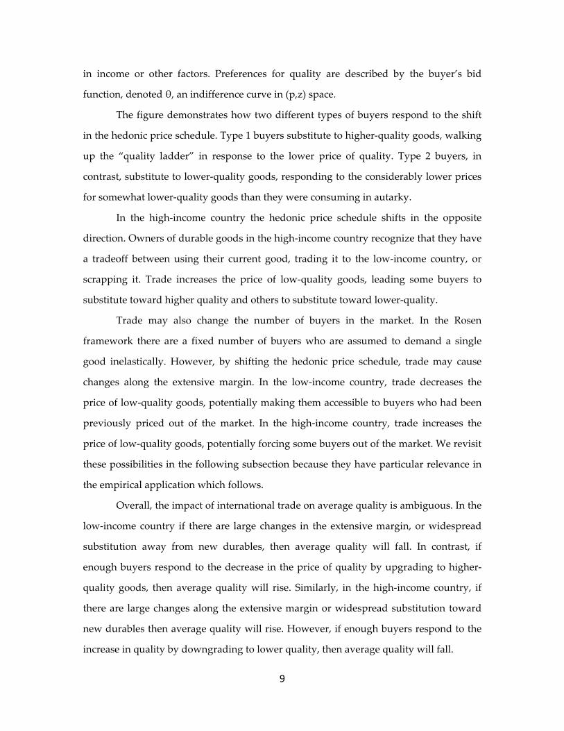
The figure demonstrates how two different types of buyers respond to the shift 

in the hedonic price schedule. Type 1 buyers substitute to higher‐quality goods, walking 

up  the  “quality  ladder”  in  response  to  the  lower  price  of  quality.  Type  2  buyers,  in 

contrast, substitute to lower‐quality goods, responding to the considerably lower prices 

for somewhat lower‐quality goods than they were consuming in autarky.  

In  the  high‐income  country  the  hedonic  price  schedule  shifts  in  the  opposite 

direction. Owners of durable goods in the high‐income country recognize that they have 

a  tradeoff between using  their  current good,  trading  it  to  the  low‐income  country, or 

scrapping  it.  Trade  increases  the  price  of  low‐quality  goods,  leading  some  buyers  to 

substitute toward higher quality and others to substitute toward lower‐quality. 

  Trade  may  also  change  the  number  of  buyers  in  the  market.  In  the  Rosen 

framework  there  are  a  fixed number of buyers who  are  assumed  to demand  a  single 

good  inelastically. However,  by  shifting  the hedonic price  schedule,  trade may  cause 

changes  along  the  extensive margin.  In  the  low‐income  country,  trade  decreases  the 

price of low‐quality goods, potentially making them accessible to buyers who had been 

previously  priced  out  of  the market.  In  the  high‐income  country,  trade  increases  the 

price of low‐quality goods, potentially forcing some buyers out of the market. We revisit 

these possibilities in the following subsection because they have particular relevance in 

the empirical application which follows.  

  Overall, the impact of international trade on average quality is ambiguous. In the 

low‐income country  if  there are  large changes  in  the extensive margin, or widespread 

substitution  away  from  new  durables,  then  average  quality  will  fall.  In  contrast,  if 

enough buyers respond to the decrease  in the price of quality by upgrading to higher‐

quality goods,  then average quality will  rise. Similarly,  in  the high‐income  country,  if 

there are  large changes along  the extensive margin or widespread substitution  toward 

new durables then average quality will rise. However, if enough buyers respond to the 

increase in quality by downgrading to lower quality, then average quality will fall.  

10

 Implicitly  in  this  section  we  are  assuming  that  there  is  limited  scope  for 

producers  of  new  durable  goods  to  respond  to  competition  from  old  goods.5  We 

recognize, however,  that changes  in  the prices of old durable goods will affect pricing 

for new durable goods  that are  close  substitutes. This  is  reflected  in  the  smooth price 

gradient  after  trade  in  figure  3. We  assume,  however,  that  as  one moves  toward  the 

high‐end  of  the  quality  gradient,  this  effect  attenuates  to  zero.  This  is  likely  to  be  a 

reasonable approximation  in  the short‐run, where only prices can change.  In  the  long‐

run, however, producers of new durable goods will want  to,  for example,  increase  the 

quality of new goods  in order  to differentiate  them  from old goods available  through 

trade. Our analysis does not capture these long‐run responses.  

 

2.3  The Environmental Consequences of this Pattern of Trade 

This pattern of trade has important environmental implications because energy‐

using  durable  goods  are  a major  source  of  local  and  global  pollutants.  This  section 

discusses the different mechanisms by which trade affects the overall level of emissions. 

Following  the  existing  literature  on  trade  and  the  environment  (e.g.,  Grossman  and 

Krueger  1993,  Copeland  and  Taylor  2003)  we  distinguish  between  scale  and 

composition,  recasting  these  mechanisms  to  our  framework  which  emphasizes 

consumption rather than production.6 

5 For example, trade in used durable goods changes the incentives for forward‐looking firms. As first articulated by Coase  (1972) and more  recently analyzed by Esteban and Shum  (2007),  the market for used durable goods limits market power for producers. A trade pattern in which used durable goods are  traded from high‐income  to  low‐income countries will  increase  the ability of producers  in  the  high‐income  country  to  exercise market  power,  and  decrease  the  ability  of producers  in  the  low‐income  country  to  exercise  market  power.  These  dynamic  effects  are mitigated, however, when  there  are  a  relatively  large number of  firms because  each producer does  not  internalize  the  effect  current  production will  have  on  future  profits  for  other  firms. Trade will  also  affect  the market  for new durable goods by  changing  resale prices,  increasing resale prices in high‐income countries and decreasing resale prices in low‐income countries. 6 A similar distinction between consumption and production is made by McAusland (2008) which examines  theoretically  how  opposition  to  environmental  regulations  varies  with  whether pollution is generated by producers or consumers. 

11

The model implies that the direct effect of trade is to increase the number of old 

goods  in  the  low‐income  country  and decrease  the number of old goods  in  the high‐

income country. Changes  in relative prices also engender changes  in purchases of new 

goods, decreasing consumption of new goods in the low‐income country, and increasing 

consumption  of  new  goods  in  the  high‐income  country.  The  scale  effect  is  the  total 

change in the overall number of durable goods in each country. 

 In addition,  trade affects  the composition, or mix of durables  in each country. 

The  model  implies  that  old  durable  goods  will  be  exported  from  the  high‐income 

country to the low‐income country. Because older, low‐quality durable goods also tend 

to be high‐emitting, this pattern of trade potentially has  important  implications for the 

environment. How  average  emissions  change  in  both  countries  depends  on  how  the 

environmental characteristics of traded goods compare to the existing stock.  

Scale and composition effects also depend on changes in the number of agents in 

the market. As discussed  earlier,  trade  equalizes  the price of quality  across  countries, 

increasing the number of buyers in the low‐income country and decreasing the number 

of buyers  in  the high‐income  country. These  changes along  the  extensive margin will 

affect composition  if these buyers demand a different  level of quality  than the average 

buyer in the market. For example, new entrants in the low‐income country will tend to 

demand very low‐quality durable goods. If these goods are also very high‐emitting this 

can have large environmental effects. 

Another  important  factor  is  intensity  of  use.  Emissions  are  a  function  of  the 

number of durable goods, their emissions levels, and the intensity with which they are 

used.  If  intensity  of  use  varies  across  countries,  trade  will  affect  the  total  level  of 

emissions  even  if  the  total number  of durable goods  in use does not  change.  Income 

effects imply that intensity of use will tend to be higher in high‐income countries. If this 

is the case, then total intensity of use will decline as durable goods are traded from high‐

income countries to low‐income countries. 

12

For local pollutants, the magnitude of social costs depends not only on the level 

of  emissions, but also on  the  location of  emissions. One of  the  important  themes  in a 

recent  literature  in  the atmospheric  sciences  is  that marginal damages  from emissions 

can vary dramatically across locations. See, e.g., Mauzerall, et al., 2005. One of the most 

important  factors  is  the number of people nearby who are  exposed  to  the  increase  in 

ambient pollution  levels. Thus, a comprehensive analysis of  the social costs  from  local 

pollution would need to measure not only the change in total emissions, but also model 

the relationship between emissions and ambient pollution levels, and examine changes 

in levels across particular locations. 

   We have highlighted the key mechanisms by which trade in used durable goods 

will affect the environment. We now turn to a specific empirical application to quantify 

the size of these separate effects. 

  3  Background: The North American Free Trade Agreement 

NAFTA  is  a  good  candidate  for  an  empirical  study  of  the  environmental 

consequences of  trade  in durable goods  for several  reasons. First,  the volume of  trade 

within North America  is large. Total merchandise trade between the United States and 

Mexico in 2006 was $335 billion (WTO, 2007, p.17). This represents a large proportion of 

total trade, particularly for Mexico where 84.8% of all exports in 2006 went to the United 

States (WTO, 2007, p. 23). Second, the stark difference in income levels between Mexico 

and the U.S. make this is a particularly good case for testing the implications of a model 

based  on  non‐homothetic  preferences.  Third,  NAFTA  marked  a  sharp  change  from 

previous policies, allowing us to observe market behavior both with and without trade 

restrictions. Fourth,  a  substantial  literature  already  exists  about  the  environmental 

consequences of NAFTA, providing a point of comparison for our analysis.7 

7  Previous  empirical  studies  of  the  effect  of NAFTA  on  the  environment  have  found mixed results. Working prior to NAFTA, Grossman and Krueger (1993) use a cross‐country regression to show  that ambient  levels of sulfur dioxide and particulates  increase with per capita GDP at low levels of GDP, suggesting that NAFTA would improve environmental quality via an overall 

13

We restrict the analysis to cars and trucks. Vehicles are the single largest category 

of  internationally  traded  used  durable  goods,  and  the  most  important  in  terms  of 

environmental considerations. In the United States, for example, 33.8% of carbon dioxide 

emissions are derived from the transportation sector.8 Using a midpoint estimate of the 

marginal damage per  ton  of  carbon dioxide  ($15, Metcalf  2008),  this  implies  external 

costs  of  approximately  $30  billion  annually.  In  addition,  in many  cities,  vehicles  are 

responsible  for  a  substantial  proportion  of  emissions  of  local  pollutants.9 Moreover, 

restricting  our  analysis  to  a  single  class  of  durable  goods  allows  us  to  assess 

environmental quality using a consistent set of measures.  

NAFTA  came  into  effect  January  1,  1994,  immediately  eliminating  tariffs  on 

many  goods  and  establishing  a  timetable  for  tariff  reductions  on many  other  goods. 

Restrictions  for used vehicles  imports were  immediately eliminated  in Canada and the 

United States. Mexico did not  initially  eliminate  restrictions but agreed  to a  timetable 

under which restrictions would be eliminated  in five phases beginning January 1, 2009 

and ending, with complete  liberalization,  January 1, 2019.10   Gearing up  to meet  these 

changes,  Mexican  President  Vicente  Fox  surprised  many  industry  insiders  by 

accelerating  the deregulation process, eliminating  trade  restrictions  for a  large class of  increase  in  income. Harbaugh, Levinson, and Wilson  (2002) argue  that these results are  fragile. Grossman and Krueger use cross‐industry evidence to examine the impact of U.S. tariff rates and pollution abatement  costs on U.S.  imports  from Mexico,  finding no  significant effect. Levinson and Taylor (2008) examine the effect of U.S. environmental regulations on trade with Canada and Mexico, finding a robust relationship between abatement costs and import levels. For the average industry, a 1% increase in abatement costs is associated with a .2% increase in net imports from Mexico.  8 United States Department of Energy,  ʺEnergy Outlook 2008ʺ, DOE/EIA‐0383(2008), Table A18, Carbon Dioxide Emissions by Sector and Source, 2006 and 2030. 9 A large literature documents the social cost of local air pollution (see, e.g., Dockery, et al. 1993, Pope 1995, Chay and Greenstone 2003, Currie and Neidell 2005, and Chay and Greenstone 2005). Airborne pollutants  have  been  linked  to  respiratory  infections,  chronic  respiratory  illness  and aggravation of existing cardiovascular disease. 10 Our study is germane to a small literature that examines the determinants of trade restrictions for used vehicles. Pelletiere and Reinert (2004) find that among 132 countries for which data are available,  74  have  some  kind  of  restrictions  on  used  vehicle  imports.  Using  cross‐country regressions,  Pelletiere  and Reinert  (2002)  and  Pelletiere  and Reinert  (2004)  find  that  the most significant factor determining used automobile protection is the presence of domestic automobile production. 

14

used vehicles beginning August 22, 2005. Under  the new rules, 10‐15 year old vehicles 

could be imported to Mexico virtually tax free. Trade restrictions remained in place for 

vehicles less than 10 years old and more than 15 years old. In continuing to restrict the 

importation of  relatively new vehicles  the Mexican government hoped  to appease  the 

powerful Mexican Association of Automobile Distributors  (MAAD) and other political 

factions within Mexico with a vested interest in new vehicle sales.11  

This removal of restrictions marked a substantial change from previous Mexican 

policies which allowed used vehicles  to be  imported only  for agricultural use. During 

the  following  three years over 2.5 million vehicles were  imported by Mexico  from  the 

United States. This represents a small  fraction of  the vehicle stock  in  the United States 

(232 million  in 2005 according to R.L. Polk), but represents a substantial fraction of the 

vehicle  stock  in Mexico  (22 million  in 2005 according  to  INEGI). The used  car  import 

market that has evolved in response to this policy change is highly decentralized, with 

thousands of car dealers and hundreds of  thousands of citizens bringing vehicles  into 

Mexico. An account  in  the Los Angeles Times describes how Ciudad  Juarez, a border 

city  just  south of El Paso, Texas, has become a major point of  trade  for used vehicles 

entering Mexico.12 

This pattern  of  trade was  foreshadowed  by Berry, Grilli  and López‐de‐Silanes 

(1993), “If  free  trade  in used cars  is permitted,  the  relatively poor Mexican consumers 

would become a major source of demand  for used cars  from  the US and Canada. This 

would substantially drive up the price of used cars and lead wealthier consumers (in all 

countries)  to  trade  in  their old  cars more  frequently.  In  this  case  a more  complicated 

trading pattern might  emerge, with  the  increase  in North American demand  for new 

cars coming largely from US and Canadian consumers, while a large portion of Mexican 

demand is satisfied by used cars.” 

11 Only vehicles produced in the United States and Canada are eligible to be imported. Vehicles exceeding  4,500  kilograms  (e.g.  buses  and  semi  trucks)  are  not  eligible.  Diesel  vehicles  are eligible, but less than 1/5th of 1 percent of all imports during this period were diesel vehicles. 12 Los Angeles Times, “In Mexico, old U.S. Cars Find New Homes” (February 16, 2008). 

15

While  these  changes were  occurring  in  the North American  used  car market, 

trade policy for new vehicles did not change. Since 1994, NAFTA has allowed duty‐free 

trade of new vehicles and new vehicle parts as  long as content restrictions are met.  In 

2005,  the most  recent year  for which data are available, Mexico exported 506,000 new 

vehicles  to  the United States.13 Since 1994, all new vehicles  sold  in Mexico must meet 

U.S. emissions standards so emissions characteristics of new vehicles are similar in both 

countries.  

  President Fox’s policy remained in place until March 18, 2008, when restrictions 

were reinstated  for all 11‐15 year old vehicles. Thus, after  the change only 10 year old 

vehicles could be imported. In addition, the government increased the excise tax on used 

vehicles entering Mexico from 3% to 15%. This return to trade restrictions was a political 

response  to  pressure  from MAAD,  who  pointed  to  alleged  decreased  sales  of  new 

vehicles, and argued vigorously for trade restrictions, claiming that the change in policy 

was needed to, “stop the accelerated conversion of our country into the world’s biggest 

automotive garbage dump.”14 

Although this pattern of trade between the United States and Mexico is unusual 

because of the high volume of trade, there is much precedent for high‐income countries 

exporting used vehicles to lower‐income trading partners. Japan exports vehicles to over 

100 different  countries,  South Korea  exports vehicles  to Vietnam  and Russia,  and  the 

United Kingdom exports vehicles to Ireland.15 Another prominent example of a vehicle 

importing country is Peru, where over 80% of the vehicles in circulation were imported 

13  See  INEGI,  Industria Automotriz  en México,  2007, Table  3.3.2, Volumen  de  Las Exportaciones  de Automóviles y Camiones por Continente y País de Destino. 14 Associated Press, “Mexico Bans  Imports of Most Used Cars”  (March 2, 2008)  reports  that  this policy  change  has  caused  a  surge  in prices  for  vehicles  that  are  exactly  10  years  old.  In  2008 dealers in South Texas reported $500‐$800 premiums for 1998 model vehicles. 15 According to the New Zealand Herald, “Import Age Limit Plan: Car Prices To Soar” (October 16, 2006),  over  100  countries  “compete”  with  New  Zealand  to  purchase  used  cars  from  Japan. According to The Korea Herald, “Exports of Used Cars Hit Record in 2007” (April 17, 2008), South Korea exported over 220,000 used  cars and  trucks  in 2007. See also The  Irish Times, “Used Car Imports from UK hit 50,000 a Year” (July 4, 2007). 

16

as used vehicles  from  the United States and  Japan.16 Although  these accounts  suggest 

that the total volume of international trade in used vehicles is large, we are not aware of 

any  comprehensive  measures  of  global  trade.  For  example,  WTO  (2007)  tracks 

“automobile products” but does not distinguish between new and used goods. 

 

4 Empirical Analysis: Scale and Composition 

In section 4.1, we describe the vehicles that were exported from the United States 

to Mexico during the first two years after trade deregulation. This provides our measure 

of scale, the total number of vehicles on the road. In section 4.2, we compare the traded 

vehicles  to  the  stock  of  vehicles  in  both  countries,  characterizing  composition. We 

compare  the  vehicle  emissions  of  traded  vehicles  to  the  stock  of  vehicles  in  both 

countries.  In  section  4.3  we  look  within  vehicle model‐vintage  groups.  Our  dataset 

allows  us  to  identify,  at  the  vehicle  level  (using VIN  numbers), which  vehicles were 

traded as a result of trade liberalization. This degree of detail is crucial because there is 

rich heterogeneity across vehicles  in emissions  levels even among vehicles of  the same 

model and vintage.  

Our  approach  emphasizes  documenting  changes  in  quantities  rather  than 

changes  in prices. Our model  implies  that  free  trade will cause prices  for used cars  to 

increase  in  the United  States  and  decrease  in Mexico.  Examining  prices would  be  a 

valuable  test  of  the model,  and would  provide  indirect  evidence  about  trade  flows. 

Nonetheless,  for  several  reasons we  chose not  to pursue  this approach. First,  the U.S. 

used car market is very large, so we did not expect to find large price effects. Moreover, 

identification of price changes would be based primarily on changes in prices over time 

for vehicles of different vintages, and thus could be difficult to separate from other time‐

varying  factors  that affect prices. Second, no publicly‐available data exist  for used car 

prices  in  Mexico.  In  a  different  context,  Davis  (2008)  examines  used  car  prices  in 

16 See  (in Spanish) Centro de  Investigación y de Asesoría del Transporte Terrestre del Perú, “Cuarto Informe  de Observación  Pública:  Externalidades Negativas Generadas  por  la  Importación  de Vehículos Usados Sobre la Salud y la Vida de la Población en Perú”, April 2005, for details. 

17

newspaper advertisements. However, this analysis is only for Mexico City and relies on 

advertised prices which may be a poor proxy for transaction prices. Third, our objective 

is to document changes in the quantity of local and global pollutants brought about by 

international  trade. Given our  focus,  it  is crucial  to  track  the  scale and composition of 

trade flows. 

 

4.1 The Effect of Trade Deregulation on Scale 

Tables 1 and 2 describe  the vehicles exported  from  the United States  to Mexico 

between  November  2005  and  July  2008.  These  data  were  collected  by  the Mexican 

Customs  Agency  a  branch  of  the  Mexican  Ministry  of  Finance  and  represent  the 

universe of vehicles that were exported during this period. Table 1 describes vehicles by 

year traded, vintage and vehicle manufacturer. Table 2 describes the top 10 most traded 

models.17 The  customs  records describe  in detail  the  substantial  flow of used vehicles 

from the United States to Mexico during this period. Overnight the flow of used vehicles 

from the United States to Mexico changed from virtually zero to over 75,000 vehicles per 

month. Overall, 2.45 million vehicles were traded during the almost three year period.18 

Newer vehicles  are heavily  represented  among  traded vehicles. Vehicles  10‐15 

years old were eligible  to be  traded but 10‐11 year old vehicles were much more often 

traded than 14‐15 year old vehicles. Our model predicts the largest price differentials for 

very old, very low‐quality vehicles. Trade may be limited, however, by transaction costs. 

Even a huge relative price differential on a very old car may not be enough to cover the 

travel and administrative costs associated with importing a vehicle.19  

17 The most commonly traded vehicle model is the Ford Explorer, a vehicle that fell largely out of favor with U.S. consumers after a highly‐publicized recall of Firestone tires in August 2000 and claims  that  the  large number of  tread separations observed with  these  tires might be related  to vehicle design. See Krueger and Mas (2004) for details. 18 Although Central America is a large market for used vehicles from the United States, very few of  these vehicles were  likely  re‐exported  to Central America. Vehicles headed  from  the United States to Central America can bypass the expense of legalizing the vehicle in Mexico by shipping the vehicle by boat, or by driving through Mexico with a temporary permit. 19  The  Alchian‐Allen,  or  “Shipping  the  Good  Apples  Out”  theorem  points  out  that  fixed 

18

The  fact  that  relatively  newer  vehicles  are  heavily  represented  provides 

suggestive evidence about what trade in vehicles would look like under different trade 

policies. According  to NAFTA,  the North American market  for used  vehicles will  be 

completely deregulated  in  2019. Without  a household‐level model,  it  is  impossible  to 

predict what vehicles would tend to be traded under such a policy change. However, the 

observed pattern suggests that the policy might lead to substantial trade in vehicles less 

than 10 years old.  

Another striking feature of these data is the prevalence of trucks and other large 

vehicles. There are several explanations  for  this pattern. First,  this reflects  the  fact  that 

only U.S. and Canadian‐produced vehicles were eligible to be imported. In addition, oil 

prices  in  the United States were high during  the period 2005‐2008, making  these  fuel‐

inefficient  vehicles  relatively  desirable  in  Mexico  where  gasoline  prices  are  set  by 

PEMEX, the national petroleum company at less than $2.50 per gallon.20   

 

4.2 The Effect of Trade Deregulation on Composition 

Although  scale  is  clearly  important,  the  environmental  impact  of  trade  also 

depends critically on the type of vehicles that are traded. The model implies that trade 

will  cause  the price  of used  goods  to  equalize, with  an  ambiguous  effect  on  average 

vehicle  quality  in  both  countries.  In  order  to  examine  the  emissions  characteristics  of 

traded vehicles we  contacted  the California  and  the  Illinois Environmental Protection 

Agencies  to  collect vehicle  level data on  emissions and vehicle attributes. These  large 

states provided us with data  from  their used vehicle emissions programs  in 2005. For 

California, we were provided with emissions records for 7.2 million vehicles that were 

tested in 2005 under California’s Smog Check program using an ASM emissions test. For  transportation  costs  decrease  the  relative  price  of  high‐quality  goods  in  importing  countries, causing consumption to shift toward these goods. See Alchian and Allen (1964) and Borcherding and Silberberg (1978) for details. 20 According to the Mexican Energy Information System, the average price per gallon of regular unleaded gasoline in Mexico was $2.11 in 2005, $2.39 in 2006, $2.40 in 2007, and $2.20 in 2008. As a  point  of  comparison  the  average  price  in  the  United  States  in  July  2008,  according  to  the Department of Energy, Energy Information Administration, was $3.95. 

19

Illinois we were provided with  a  sample  of  835,000 vehicles  that were  tested  in  2005 

using  an  IM240  test. We  use  these  records  to  estimate  average  emissions  levels  for 

vehicles  of  different  manufacturers  and  vintages.  For  vehicles  which  were  tested 

multiple times, we use data on the first vehicle emissions test for each vehicle. In Section 

4.3 we return  to  these multiple  tests and are able  to  test directly  if  traded vehicles are 

more likely to have failed emissions testing. 

Let   denote the average emissions level among all vehicles from manufacturer 

j and vintage t. Vehicles produced in 1976 or before are grouped together, and vehicles 

produced after 2005 are grouped  together,  so  the  set of all vintages, T,  includes 1976‐

2005. We  focus  on  all manufacturers  for which  there were more  than  1,000,000  total 

registered  vehicles  in  the United  States  as  of  2005. Other  vehicle manufacturers  are 

included  in  an  “other”  category.21  Let  J  denote  this  set  of  30 manufacturers.  For  the 

results  reported  below,  we  calculated  the    vector  using  the  emissions  data  from 

California,  the  largest  and  arguably  the most  reliable  set  of  emissions measures. We 

have also examined  results based on emissions  factors  calculated using data  from  the 

Mexico City Emissions Testing Program and results are qualitatively similar, providing 

evidence  that  our  results  are  not  driven  by  selection  of  a  particular  set  of  emission 

factors. 

Composition  is measured by  comparing  the emissions  characteristics of  traded 

vehicles with  the emissions characteristics of  the stock of vehicles  in  the United States 

and Mexico,  

Average Emissions of Traded Vehicles,

 

Average Vehicle Emissions in U. S.,

 

21 Our manufacturers  include Acura, BMW, Buick, Cadillac, Chevrolet, Chrysler, Dodge, Ford, GMC,  Honda,  Hyundai,  Infiniti,  Isuzu,  Jeep,  Kia,  Lexus,  Lincoln,  Mazda,  Mercedes‐Benz, Mercury,  Mitsubishi,  Nissan/Datsun,  Oldsmobile,  Plymouth,  Pontiac,  Saturn,  Toyota, Volkswagen, and Volvo. 

20

Average Vehicle Emissions in Mexico,

. 

Here    denotes  the  proportion  of  traded  vehicles  of  each manufacturer  and 

vintage, and   and   denote the proportion of the vehicle fleet of each manufacturer 

and vintage in the United States and Mexico. We measure the empirical distribution of 

vehicles in the United States and Mexico using ancillary datasets. For the United States, 

we obtained data from R.L. Polk that describe the distribution of registered vehicles  in 

the United States as of 2005 by manufacturer and vintage. For Mexico, describing  the 

distribution of vehicles was more challenging.22 We filed the equivalent of a Freedom of 

Information Act  request with  the Mexican Ministry  of  Public  Safety  via  the Mexican 

Federal Institute for Access to Public Information. In response to our request, we were 

provided with  a document describing  the distribution  of vehicles  in Mexico  by  state, 

vintage, and manufacturer as of 2008. Similar data for 2005 are not available. 

Table 3 presents the composition results. The table reports mean emission levels 

for hydrocarbons, carbon monoxide and nitrogen oxide, as well as vehicle vintage. The 

results  imply  that NAFTA  led  to a decrease  in average emissions of  local pollutants  in 

both  the United  States  and Mexico. Compared  to  the  stock  of  vehicles  in  the United 

States, traded vehicles emit higher levels of all three local pollutants. The differences are 

substantial, ranging from 6% for carbon monoxide to 20% for nitrogen oxide. Compared 

to  the  stock of vehicles  in Mexico,  traded vehicles  emit  lower  levels of  all  three  local 

pollutants. Again  the  differences  are  substantial,  ranging  from  approximately  3%  for 

nitrogen oxide to 38% for carbon monoxide.23  

22 Although vehicle registration is required in all parts of Mexico, registries are maintained at the state level and the Mexican National Statistics Institute compiles total vehicle counts by state and year,  but  not  by  vintage  or manufacturer. Another possibility would  be  to use  commercially‐available  data.  R.  L.  Polk  maintains  data  about  registered  vehicles  in  Mexico  by  vehicle manufacturer, but not by vintage. 23  The  table  indicates  a  clear  ordering  of  vehicles  by  age.  The  stock  in  the  United  States  is considerably newer than the stock of vehicles in Mexico, with traded vehicles in between. Older vehicles  tend  to emit higher  levels of emissions because of both vintage effects and age effects, though  engineering  studies  (e.g. Bishop  and  Stedman,  2008)  have  tended  to  find  that  vintage effects are more important. This suggests that these differences in local emission levels are likely 

21

The  table  also  reports  results  for miles‐per‐gallon,  vehicle weight,  number  of 

cylinders, and engine size.24 Carbon dioxide emissions are proportional to total gasoline 

consumption and  these measures directly or  indirectly measure vehicle  fuel‐efficiency. 

Traded vehicles are marginally less fuel efficient on average than the stock of vehicles in 

both  countries.  As  a  result,  trade  increases  fuel  efficiency  in  the  United  States,  and 

decreases  fuel  efficiency  in  Mexico  City.  The  differences  are  small.  Whereas  local 

emissions vary across columns by as much as 30‐40%, the differences in miles‐per‐gallon 

vary  by  less  than  3%,  indicating  that  composition  effects  are  likely  to  play  a much 

smaller role for global pollutants. 

 

4.3 Vehicle‐Level Heterogeneity in Emission Levels 

The previous  subsection  illustrated  that  the vehicles  exported  from  the United 

States  to Mexico  were  higher‐emitting  on  average  than  the  stock  of  vehicles  in  the 

United States and lower‐emitting than the stock in Mexico. Our data, however, allow us 

to  refine  the analysis  further. For  each vehicle  that was  emissions  tested  in California 

and  Illinois  in  the  year  2005, we  know  the  vehicle  identification  number  (VIN).  By 

merging  these  records with  the  customs  records  of  traded  vehicles, we were  able  to 

identify  the  subset  of  vehicles  that  were  subsequently  exported  to  Mexico.  This 

information  is  crucial  for  examining  changes  in  composition  because  even  within 

vehicles of the same model and vintage there is large heterogeneity in emissions levels.  

In this section we test hypotheses concerning differential emission levels between 

U.S.  vehicles  and  vehicles  that were  not  exported  to Mexico  at  the  vehicle  level.  In 

particular, we  run  regressions  controlling  for manufacturer, model,  and vintage  fixed 

effects, 

to be persistent over time. 24 We  imputed miles‐per‐gallon  for  each  vehicle  using  vintage,  vehicle weight,  cylinders,  and engine size. Using data from the Department of Transportation, National Highway Traffic Safety Administration,  for  each  vintage  1978‐2005 we  estimated  a  separate  regression  of miles‐per‐gallon on weight, cylinders and engine size and  then used  the estimated coefficients  to predict miles‐per‐gallon for each vehicle in the emissions testing data. 

22

y 1 δ ω σ ε . 

We estimate a variety of specifications using as the dependent variable the same 

measures of emissions and vehicle characteristics used in the previous subsection. In all 

specifications,  the  coefficient  of  interest    corresponds  to  an  indicator  variable  for 

whether  the  vehicle  was  subsequently  exported  to  Mexico.  A  positive  coefficient 

indicates  that  vehicles  exported  to Mexico  have  higher  levels  of  y. We  report  results 

from  specifications  that control  for vintage  indicators,  δ , as well as  specifications  that 

control for manufacturer/vintage interactions, ω , and even model/vintage interactions, 

σ .25 In this fully  interacted specification   describes how y varies compared to other 

vehicles of the same model and vintage. 

Table  4  reports  coefficients  and  standard  errors  corresponding  to  36  separate 

OLS regressions. Across pollutants and specifications we find evidence that the vehicles 

exported to Mexico have higher local emission levels. Columns (3) and (7) report results 

with the full set of model/vintage interactions. Compared to other vehicles of the same 

model and vintage,  traded vehicles have emissions  levels  that are  significantly higher 

than vehicles not sent to Mexico. The effect remains in column (4) after controlling for a 

quadratic  in mileage,  indicating  higher  emissions  for  exported  vehicles  even within 

vehicles of the same make, vintage, and mileage. We also examine odometer readings as 

a  separate  dependent  variable.  Controlling  for  model/vintage  interactions,  vehicles 

exported  to Mexico  have  on  average  almost  10,000 more miles.  Consistent with  our 

model,  these  results provide evidence  that  low‐quality vehicles are disproportionately 

desirable in Mexico. 

  The  table  also  reports  coefficients  corresponding  to miles‐per‐gallon  and other 

vehicle  characteristics predictive of  carbon dioxide  emissions. Controlling  for vintage, 

traded vehicles are  less  fuel efficient, heavier, with more cylinders, and  larger engines 

than  the stock of vehicles  in California. This  is consistent with  the pattern observed  in  25 Model  is measured  using  the  5th  digit  of  the  VIN  number  as  assigned  by  each  individual manufacturer. This classification of model distinguishes between, for example, the Ford Windstar (a minivan) and  the Ford F‐Series  (a  truck), but does not distinguish,  for example, between  the Ford F‐150 and the Ford F‐250. 

23

table 2 that minivans, SUVs, and trucks are heavily represented among traded vehicles. 

After controlling for manufacturer/vintage or model/vintage interactions the coefficients 

become much smaller. 

Table  5 presents  coefficient  estimates  from  additional  regressions using  as  the 

dependent variable whether or not the vehicle has failed emissions testing. Vehicles that 

emit extremely high levels of pollutants are particularly important for the environment 

because  it has been  shown  that  these vehicles  contribute a  large proportion of overall 

emissions.  In  these  regressions  the  dependent  variable  is  an  indicator  variable  for 

whether  the vehicle  failed  emissions once,  twice,  and  three or more  times,  as well  as 

whether  the  vehicle  was  a  “gross  polluter”  once,  twice,  and  three  or  more  times. 

According  to  California  law,  a  “gross  polluter”  is  a  vehicle  that  exceeds  twice  the 

allowable emissions for at least one pollutant. The results indicate that exported vehicles 

are more  likely  to  be  super‐emitters.  The magnitude  of  the  differences  is  large.    For 

example,  after  controlling  for model/vintage  fixed  effects,  exported  vehicles  are  over 

four times more  likely to have failed emissions testing three times, and over five times 

more  likely  to have been declared a gross polluter  three or more  times. This pattern  is 

consistent with vehicles being  exported  to Mexico after  they become  too  expensive  to 

maintain according  to emissions  standards. This could also be evidence of differential 

asymmetric  information,  with  Mexican  buyers  less  able  to  identify  high‐emitting 

“lemons”. 

  Overall  the  results  imply  that exports are “browner”  than  the average  stock  in 

the  United  States.  We  conclude  based  on  the  California  and  Illinois  samples  that 

exported vehicles tend to be significantly higher‐emitting than other vehicles. This effect 

remains after controlling for vintage, manufacturer, and model. Our model implies that 

low‐quality vehicles are disproportionately desirable  in Mexico, and  the  trade pattern 

reflects this.  

 

24

5  The Behavioral Response: New Vehicle Sales and Vehicle Retirement 

  According to our model, trade  liberalization causes prices of  low‐quality (used) 

goods to  increase  in the high‐income country and decrease  in the  low‐income country. 

In  the  high‐income  country,  high‐quality  goods  (new)  goods  become  relatively  less 

expensive, and consumption of these goods  increases. In addition, because  low‐quality 

goods have become relatively more expensive, households hold on to them longer, and 

one would expect vehicle retirement rates to decrease. See, e.g. Gruenspecht (1982).   In 

the  low‐income country, the results are exactly the opposite. High‐quality (new) goods 

become  relatively more  expensive,  and  consumption  of  these  goods  decreases.  Low‐

quality (used) goods become less expensive, and vehicle retirement rates increase. These 

changes  in  behavior  are  potentially  important  because  they  may  mitigate  the 

environmental impact of trade. 

  In  this  section  we  examine  vehicle  purchase  and  retirement  behavior  using 

detailed  data from both countries. The section has three main results. First, NAFTA did 

not meaningfully affect the number of registered vehicles  in the United States. Second, 

vehicle retirement rates are substantially lower in Mexico than the United States. Third, 

there is little evidence that trade decreased sales of new vehicles in Mexico.  

 

5.1  Vehicle Retirement in the United States 

  In this subsection we examine changes  in the stock of registered vehicles  in the 

United States during the period 2003 to 2007. We observe increased exit rates among 10‐

15 year old vehicles during  the post‐NAFTA period, but  the  increase  is much  smaller 

than the flow of vehicles to Mexico. We conclude that most of the vehicles exported to 

Mexico during this period were either vehicles that would have been retired otherwise 

or  vehicles  that were  already  retired  (i.e.  not  registered).  This  is  consistent with  our 

evidence  from  Section  4.3  that  very  low‐quality  vehicles  are more  likely  than  other 

vehicles to be traded.  

25

As  a  result,  the  elimination  of  trade  restrictions  in Mexico  led  to  little  or  no 

impact on the number of registered vehicles in the United States. This “zero effect” for 

scale  in  the United  States  is  not  surprising. The  stock  of used  vehicles  in  the United 

States  is  large,  so  increased demand  for used vehicles  is unlikely  to have  raised used 

vehicle prices more than a few hundred dollars per vehicle. Moreover, the capital cost of 

used  vehicles  is  only  one  part  of  the  costs  of  operating  a  vehicle  (e.g. maintenance, 

insurance, gasoline, etc) and in the United States the elasticity of vehicle ownership with 

respect  to  these costs  is  likely very  low.  In short,  it  is hard  to  imagine  trade  leading a 

large number of households in the United States to reduce the number of vehicles they 

own.  

Figure 4: Exit Rates by Vehicle Age in the United States 

 

Figure  4  plots  exit  rates  by  vehicle  age  in  the United  States  before  and  after 

NAFTA.26 The overall pattern  is consistent with previous studies of vehicle retirement 

26 These data were obtained from R.L. Polk & Company in April 2008. Exit rates were calculated by  calendar year and vehicle age  as  follows. Let  v denote vehicle vintage  (e.g.  1991) and  let  t denote calendar year. We calculated the exit rate for vehicles age t‐v for year t, as the percentage change in the number of vehicles of vintage v between year t‐1 and t. 

0.0

5.1

.15

2 3 4 5 6 7 8 9 10 11 12 13 14 15 16 17 18 19 20

Source: R.L. Polk & Company.

Before NAFTA (10/03 - 10/05)After NAFTA (10/05 - 10/07)

26

patterns. Annual exit rates increase with vehicle age from less than 2% for vehicles that 

are  4‐5 years old  to more  than  10%  for vehicles over  15 years old. The  figure  reveals 

higher exit rates after NAFTA for vehicles 10‐15 years old. Five out of the six differences 

are statistically significant at the 1%  level. Across vehicle ages, retirement rates tend to 

be higher during  the post‐NAFTA period, perhaps due  to  the gasoline price  increases 

during this period. However, we take the disproportionately large increases among 10‐

15 year old vehicles as evidence of trade with Mexico. 

However,  the  increase  in  exit  rates  for vehicles  10‐15 years old  implies only  a 

small  overall  decrease  in  the  number  of  vehicles  in  the United  States.  Even without 

controlling for the apparent overall increase in exit rates during the post‐NAFTA period, 

these  results  imply only approximately 180,000 additional exits annually among 10‐15 

year  old  vehicles  relative  to  the  earlier  period.  The  number  of  exits  is  considerably 

smaller  than  the  1,000,000  vehicles  per  year  that were  exported  annually  to Mexico 

during  this period,  suggesting  that most of  the vehicles  that were exported  to Mexico 

would  have  been  retired  otherwise  or were  drawn  from  the  stock  of  already  retired 

vehicles. 

These data underestimate the total number of exits because there is a lag between 

when a vehicle exits and when it is removed from the R.L. Polk database.27 Results are 

similar, however, when we  instead define  the post‐NAFTA period as October 2006  to 

October 2007, a later period which includes exits both from the October 2006 to October 

2007  period  and  delayed  exits  from  October  2005  to  October  2006.  Using  this 

specification  the  results  imply 315,000 additional exits annually among 10‐15 year old 

vehicles relative to the earlier period.  27 The R. L. Polk data are based on vehicle registrations, and vehicles are registered only once a year. Thus, for example, if a vehicle is registered in January and then exported in February it will not disappear from the vehicle registry until the following January. In addition, R.L. Polk allows for  another  6  months  past  the  due  date  of  registration  before  dropping  a  vehicle  from  its database. As a result, in some cases a vehicle that is exported will not be reflected as “missing” until 18 months later. Assuming that exports are uniformly distributed across years and months and assuming that vehicle registrations are uniformly distributed throughout the year (consistent with our conversations with R. L. Polk), exits October 2005 to October 2006 will include only 25% of actual exports, whereas exits October 2006 to October 2007 will include 96%. 

27

These results highlight the immense size of the used vehicle market in the United 

States. During  the period  2003‐2007,  5.9 million  vehicles were  retired  annually  in  the 

United States, 2.1 million vehicles 10‐15 years old. This provides a large potential stock 

of  vehicles  for  export,  even without  dipping  into  the  stock  of  registered  vehicles. A 

relatively small fraction of these castoffs can represent a large number of vehicles for a 

smaller country like Mexico. 

 

5.2  Differential Vehicle Retirement Rates in the United States and Mexico  

The model implies that retirement rates will be higher in the United States than 

Mexico.  In  autarky,  old  durable  goods  are  relatively  inexpensive  in  the  high‐income 

country, so when faced with repair costs, agents are more likely to retire the good. In the 

low‐income  country,  old  durable  goods  are  relative  expensive,  so  when  faced  with 

repair costs, agents are less likely to retire the good.  

Figure 5 describes  the age distribution of vehicles  in both countries. Consistent 

with the predictions of the model, vehicles in Mexico tend to be much older. The average 

age of vehicles  in  the United States  is 9.4 years compared  to 13.5 years  in Mexico. The 

distribution  implies  dramatically  different  vehicle  retirement  behavior  in  the  two 

countries. The implied mean annual exit rate for 10‐30 year old vehicles is 12.2% in the 

United States and only 3.8% in Mexico. 

 

28

Figure 5: The Age Distribution of Vehicles 

  

5.3  Vehicle Sales in Mexico 

Our model  implies  that  the  influx  of  relatively high‐quality used vehicles will 

cause households  in Mexico to substitute away from new vehicles. Indeed, MAAD has 

been  a  vocal  opponent  to  liberalization,  and  claims  that  NAFTA  has  reduced  sales 

considerably.28    In  this  subsection we  examine  the  evidence  from  new  vehicle  sales, 

finding no  evidence of decreased  sales. The one possible  exception  is  subcompact  car 

sales, which indeed drop during the post‐NAFTA period, though sales appeared to be in 

decline even prior  to  trade deregulation. Overall,  the evidence  from new vehicle  sales 

suggests that the 10‐15 year old used vehicles were not an attractive alternative for most 

buyers of new vehicles.  

28 Recent publications from the Mexican Association of Automobile Distributors describe in detail the environmental and commercial  threats  from  free  trade  in used vehicles. See, e.g., “Trade  in Very  Old  Used  Cars:  A  Challenge  for  Air  Quality”  (“El  Comercio  de  Autos  Usados  de  Gran Antigüedad:  Un  Reto  a  la  Calidad  del  Aire  en  las  Cuencas  Atmosféricas  de  la  Frontera  de  EUA  y México”), August 2007. Our study is the first full‐scale attempt to measure empirically the impact of NAFTA on new vehicle sales. 

0.2

.4.6

.81

0 10 20 30Age

Registered Vehicles in the United StatesRegistered Vehicles in Mexico

29

Figure 6. Monthly Sales of New Vehicles in Mexico 

 

Figure 6 plots monthly sales of new vehicles in Mexico during the period January 

2001  to December 2007, as well as a  fitted  cubic polynomial  in  time with  intercept at 

August 2005 when the market for used vehicles was  liberalized. Based on the plot  it  is 

difficult  to make  strong  statements  about  the  impact  of  trade  deregulation  on  sales. 

Overall,  vehicle  sales  post‐NAFTA  are  similar  to  sales  pre‐NAFTA.  There  is  a 

pronounced season pattern  to sales, which will be  taken  into account  in  the regression 

analysis which follows.  

Figure  7  plots monthly  sales  of  new  vehicles  in Mexico  by  vehicle  category. 

Whereas  sales  of  subcompacts  decrease  steadily  after  August  2005,  sales  for 

subcompacts, luxury cars, and light trucks and SUVs increase. With their relatively low 

quality design and few features, subcompacts are likely the closest substitute to the used 

vehicles  from  the United States, and  thus  it  is not  surprising  that  this category would 

have  been most  affected.  Still,  we  are  hesitant  to make  definitive  statements  about 

causality  particularly  because  the  decline  in  subcompact  sales  appears  to  begin  even 

prior to trade deregulation.  

6080

100

120

140

Mon

thly

Sal

es (i

n th

ousa

nds)

2001 2002 2003 2004 2005 2006 2007 2008Source: INEGI, La Industria Automotriz en México, 2002-2008.

30

Figure  7.  Monthly  Sales  of  New  Vehicles  in  Mexico  by  Vehicle  Category 

 

  Table  6  reports  coefficients  and  standard  errors  from  an  analogous  regression 

analysis. Monthly  sales  of  new  vehicles  in Mexico  (in  logs)  are  regressed  on month 

indicator  variables,  a  polynomial  time  trend,  and  an  indicator  for  after NAFTA.  To 

control  for  aggregate  changes  in  demand, we  also  include  the  growth  rate  of  GDP 

(available quarterly)  from  the Mexican National Statistics  Institute, National System of 

Accounts. For second, third, and fourth order polynomials, the coefficient on NAFTA for 

total sales is near zero and not statistically significant. The null hypothesis of a 10% drop 

in  total  vehicle  sales  can  be  rejected  at  the  2%  level  across  specifications.  For 

subcompacts  the  coefficient  is  negative  and  near  5%,  but  not  statistically  significant. 

Compact and luxury car sales increase in all specifications.  

In  future  work  it  would  be  valuable  to  examine  trade’s  general  equilibrium 

model based on structural estimates of household‐level vehicle demand. See, e.g. Berry, 

Levinsohn,  Pakes  (1995),  Goldberg  (1999),  and  Bento,  Goulder,  Jacobsen,  and  von 

Haefen (2008).  One potential challenge of estimating such a model in this context is the 

2030

4050

60M

onth

ly S

ales

(in

thou

sand

s)

2001 2002 2003 2004 2005 2006 2007 2008

Subcompact Cars

1015

2025

30M

onth

ly S

ales

(in

thou

sand

s)

2001 2002 2003 2004 2005 2006 2007 2008

Compact Cars2

34

56

7M

onth

ly S

ales

(in

thou

sand

s)

2001 2002 2003 2004 2005 2006 2007 2008

Luxury and Sports Cars

1020

3040

50M

onth

ly S

ales

(in

thou

sand

s)

2001 2002 2003 2004 2005 2006 2007 2008

Light Trucks and SUVs

Source: INEGI, La Industria Automotriz en México, 2002-2008.

31

difficulty of acquiring necessary Mexican data. Structural models of vehicle demand in 

the  United  States  have  been  successful,  in  part,  because  researchers  have  access  to 

detailed micro‐level datasets like the National Household Travel Survey (NHTS) and the 

Consumer Expenditure Survey  (CES). There  is no dataset  in Mexico comparable  to  the 

NHTS. The Mexico  equivalent  to  the CES,  the National Survey of Household  Income 

and  Expenditures  includes  basic  household  demographics  and  information  about 

expenditures on vehicles, vehicle maintenance, vehicle  insurance, and vehicle  licensing 

and  fees,  but  does  not  include  the  manufacturer,  model,  or  vintage  of  household 

vehicles.  

 

5.4  An Illustration of How Trade Can Increase Lifetime Carbon Emissions 

In Section 5.1, we presented evidence that indicates that NAFTA had little effect 

on the total number of vehicles in circulation in the United States. Section 5.2 examined 

the distribution of vehicle age in both countries, finding evidence of dramatically lower 

retirement  rates  in Mexico.  Finally,  Section  5.3  showed  that  changes  in  new  vehicle 

purchases in Mexico are too small to considerably offset the large influx of vehicles from 

the United States. These results together indicate that overall NAFTA is associated with 

a  substantial  net  increase  in  the  number  of  vehicles  in  circulation.  In  this  section we 

evaluate  the  implications  of  this  increase  for  lifetime  greenhouse  gas  emissions. 

Although our analysis provides much of the information required for these calculations, 

these  results do  require us  to make  a number of  additional  assumptions, particularly 

about vehicle utilization.29  As a result, we refer to these results as an “illustration” and 

these results should be interpreted with caution. 

We  consider  both  short‐run  and  long‐run  thought  experiments.  For  the  short‐

run,  we  examine  the  change  in  annual  global  carbon  emissions  that  results  from 

increasing the number of vehicles in Mexico by 1,000,000. This corresponds closely with 

the annual  level of  imports during  the period 2005‐2008. For  the  long‐run  illustration,  29 If the micro data existed, Goldberg’s (1999) structural model of the vehicle ownership decision and the utilization (miles driven) decision could be used to estimate the social cost of trade.

32

we calculate the lifetime increase in carbon emissions from these vehicles. The long‐run 

cumulative  impact  of  trade  is  particularly  important  in  this  context  because  vehicle 

retirement  rates  in Mexico are  low,  so  these 1,000,000 vehicles  continue  to be used  in 

Mexico for many years. 

Short‐run  carbon  emissions  are  the product  of number  of  vehicles, number  of 

miles driven annually, and emissions per mile: 

  (1)

Scale enters through the number of vehicles, and composition enters emissions per mile. 

Long‐run carbon emissions are total lifetime emissions, 

∞

  (2)

where  λ  is  the  vehicle  retirement  rate.  For  λ we use  .038,  the  average  annual 

retirement  rate  for vehicles 10‐30 years  from  section 5.2. For miles driven, we use  the 

average number of miles driven annually per vehicle  in  each  country. Vehicles  in  the 

United  States  travel  an  average  of  12,408  miles  annually  compared  to  6,100  miles 

annually in Mexico.30 We would have preferred instead to use measures of miles driven 

that vary by vehicle model and vintage, but with no vehicle‐level information available 

on miles driven in Mexico, this was not possible.  

  Table 7 reports the short‐run and long‐run increases in carbon. The impact of one 

year  of  trade  is  substantial,  increasing  carbon  dioxide  emissions  by  2.6 million  tons 

annually. To put  these results  in some context, using  these same methods  total annual 

emissions of carbon dioxide from vehicles in the United States and Mexico is 1.2 billion 

tons and 56 million  tons,  respectively. Using $15 per  ton  for  the  social  cost of  carbon 

30  U.S.  Department  of  Transportation,  Federal  Highway  Administration,  ʺHighway  Statistics  2006ʺ, Section V: Roadway Extent, Characteristics, and Performance, Table VM‐1. No analogous survey‐based statistic  is available  for Mexico. However, annual gasoline consumption  indicates that vehicles tend to be used less intensively. Gasoline consumption in Mexico in 2007 totaled 8.6 billion  gallons  (SIE,  2008). Using  average miles  per  gallon  from  Table  3,  this  implies  that  the average  vehicle  in Mexico  travels  6,100 miles  annually.  Vehicles  are  used  less  intensively  in Mexico for many reasons including lower income levels, lower quality roads and highways, and differences in commuting patterns. 

33

dioxide following Metcalf (2008), this  implies social costs of $39 million. Using $85 per 

ton  for  the  social  cost  of  carbon  dioxide  following  Stern  (2007),  social  costs  are  $219 

million.  The  long‐run  results  are  considerably  larger.  The  total  lifetime  increase  in 

carbon dioxide emissions from these vehicles is 67.7 million tons. Total social cost ranges 

from  $1.02  billion  to  $5.76  billion depending  on  the  value used  for  the  social  cost  of 

carbon.  

It  is  important  to  emphasize  that  these  thought  experiments describe  trade  in 

vehicles during only a  single 1‐year period. To  calculate  the  total  lifetime  impact of a 

permanent policy change it would be necessary to calculate and take the sum of lifetime 

emissions for each successive wave of imports. Moreover, because of the large stock of 

vehicles  in  the United  States,  it  is  not  unrealistic  to  believe  that  trade  flows  of  this 

magnitude  from  the United  States  to Mexico  could  continue  at  this  rate  over  a  long 

period of time. The stock of vehicles in the United States is approximately 10 times the 

stock  in  Mexico,  and  a  flow  of  1,000,000  annually  can  be  maintained  simply  by 

siphoning off a fraction of the vehicles that otherwise would have been scrapped. 

These  results provide a valuable preliminary assessment of  the  total  impact of 

U.S.‐Mexico trade on carbon dioxide emissions. However,  it  is  important to emphasize 

that  these  numbers  are  based  on  several  assumptions, many  of  which  can  be  only 

partially verified empirically. First, we are assuming  implicitly that prior to driving an 

imported used  car, Mexicans were generating no  carbon dioxide  from  transportation. 

For  households  substituting  from  high‐occupancy  public  transportation,  this  is  a 

reasonably  accurate  approximation. However,  for households  substituting  away  from 

low‐occupancy public  transportation or  from  shared private vehicles,  there will be an 

offsetting decrease in vehicle emissions.  

Second, these results describe the social cost from carbon dioxide emissions, but 

not the social cost from emissions of local pollutants. There is reason to believe that the 

social cost  from  increased ambient pollution  levels could be  large  relative  to  the costs 

associated with climate change. For example, World Bank  (2002)  finds  that  the annual 

benefits of a 10 percent  reduction  in ozone and particulates  in Mexico City would be 

34

approximately $882 million (in 2006 U.S. dollars). A more comprehensive analysis of the 

social costs of trade in used vehicles would track vehicles after they enter Mexico, model 

the  relationship  between  emissions  and  ambient pollution  levels,  and  incorporate  the 

social costs of the resulting increases.  

 

6 Conclusion  

  Wealthy  nations  demand  a  range  of  high‐quality  transportation  equipment 

(trucks,  trains,  buses, boats,  and  planes),  as  well  as  residential  durable  goods  (air 

conditioners,  clothes washers,  etc),  commercial durables  (computers,  lighting, heating 

and  cooling  equipment,  etc)  and  industrial  durables  (power  generating  equipment, 

metalworking equipment, construction machinery, etc). These durable goods depreciate 

in quality over time.  Poorer nations want to purchase similar durable goods but due to 

income effects desire lower quality. From a societal perspective, there are gains to trade 

from shipping used durable goods from rich countries to poorer countries. 

In  this  paper  we  argued  that  this  pattern  has  large  implications  for  the 

environment.  As  we  discuss  in  the  paper,  the  effect  of  trade  on  average  and  total 

emissions depends  on  the  relative magnitude  of  scale  and  composition  effects. Trade 

provides  rich  countries  with  an  outlet  for  low‐quality  durable  goods.  Because  low‐

quality durables are typically also high‐emitting, this tends to decrease average and total 

emissions  in  rich  countries.  In poor  countries,  trade  increases  the  number  of durable 

goods,  but may  also  improve  the quality  of  the  stock. Whether  or not  this  change  in 

composition  is  large enough  to offset  the scale effect depends on  the characteristics of 

the initial stock of durable goods and other factors. 

In the empirical analysis we focused on the deregulation of the market for used 

cars and trucks following NAFTA. Scale effects are immediate and large and magnitude, 

with millions  of  vehicles  exported  from  the United  States  to Mexico  during  the  first 

years of  trade. Composition effects are also  large. For  local pollutants,  traded vehicles 

have significantly higher emissions than the stock in the United States, and significantly 

35

lower emissions than the stock in Mexico. As a result, trade decreased average emissions 

of  local pollutants  in both countries. For carbon dioxide emissions, composition effects 

are much  smaller, with  traded vehicles marginally  less  fuel‐efficient  than  the  stock  in 

either country.  

Total emission levels decrease in the United States and increase in Mexico, with 

global  carbon  dioxide  emissions  increasing. Whereas  trade  has  led  to  no  discernible 

decrease in the number of vehicles in circulation in the United States, it has led to a large 

increase  in  the number of vehicles  in Mexico. Furthermore, because vehicle retirement 

rates  are  low  in Mexico,  these vehicles will  continue  to be used  for many years. This 

pattern  is  likely  to  be  the  case  not  just  for NAFTA,  but  for North‐South  trade more 

generally. Although the magnitude of scale and composition will differ across contexts, 

this tendency of durable good lifespans to be increased by trade is likely to be repeated 

elsewhere as barriers to trade continue to fall. 

The  broader  conclusion  of  our  paper  is  that  policymakers  in  conducting 

economic  analysis  of  environmental  policies  ought  to  take  careful  account  of  the 

implications of their policies for trade in used durables. This is particularly important for 

global pollutants  such  as  carbon dioxide where domestic policies designed  to  reduce 

emissions  can  be  easily  undermined  by  emissions  increases  abroad.  As  a  result, 

unilateral  policies  aimed  at  reducing  greenhouse  gas  emissions  may  not  achieve 

aggregate gains when fuel inefficient vehicles can be traded. 

Our results also have implications for predicting likely unintended consequences 

induced  by  pending  United  States  climate  change  mitigation  legislation. Today, 

California  is  leading  an  effort  to  unilaterally  reduce  its  greenhouse  gas  emissions 

through AB32  legislation. Economists have pointed out  that “leakage”  can undermine 

the  aggregate  benefits  of  this  initiative. Leakage  takes  place when  regulation  in  one 

spatial sector, such as California, leads to migration of polluting activity away from the 

regulated area to an unregulated area. 

36

   Given  that  the  transportation  sector  is  a  major  producer  of  carbon  dioxide 

emissions,  the  Congress  continues  to  wrestle  with  raising  fuel  economy  (CAFE) 

standards  or  raising  gasoline  taxes. Our  results  speak  directly  to  the  differential 

implications of  these  two policies. If CAFE standards  increase sharply, exports of used 

vehicles  to  Mexico  will  decline. As  articulated  by  Gruenspecht  (1982),  new  vehicle 

regulations  increase  the  cost  of  new  vehicles,  causing  households  to  delay  new  car 

purchases. This would  increase demand  for used cars  in the United States, bidding up 

the price, and leading fewer used cars to be shipped to Mexico. 

  In contrast, increasing the gasoline tax would increase exports of used vehicles to 

Mexico. A gasoline  tax  in  the United States would make  large,  fuel  inefficient vehicles 

relatively more desirable  in Mexico. We have  shown  that  it was already  the  case  that 

many of the vehicles exported to Mexico between 2005 and 2008 were trucks, minivans, 

and  SUVs.  This  pattern would  almost  certainly  be  exacerbated  by  an  increase  in  the 

gasoline  tax,  causing  further  decreases  in  emissions  in  the United  States  and  further 

increases in emissions in Mexico. Thus, the broader conclusion of our analysis is that the 

composition of trade can change sharply as U.S incentives change.  

   

37

References 

Alchian, Armen A.  and Allen William  R., University  Economics.    Belmont, Calif.: Wadsworth, 1964.  

Antweiler, W., Copeland, B. and Taylor, S. “Is Free Trade Good for the Environment?”American Economic Review, 2001, 91 (4), 877‐908.  

Bento, Antonio M., Larry Goulder, Mark R. Jacobsen, and Roger H. von Haefen, “Distributional and  Efficiency  Impacts  of  Increased  U.S.  Gasoline  Taxes”  American  Economic  Review, forthcoming. 

Berry, Steven, Vittorio Grilli and Florencio López‐de‐Silanes, “The Automobile Industry and the Mexico‐U.S.  Free  Trade  Agreement”  in  P.  M.  Garber,  ed.,  The  Mexico‐U.S.  Free  Trade Agreement, Cambridge, MA: MIT Press, 1993. 

Berry,  Steven,  James  Levinsohn  and Ariel  Pakes.  “Automobile  Prices  in Market  Equilibrium” Econometrica, 1995, 63(4), 841‐890. 

Bishop, Gary A.  and Donald H.  Stedman,  “A Decade  of On‐Road  Emissions Measurements” Environmental Science and Technology, 2008, 42(5), 1651‐1656. 

Borcherding, Thomas E.  and Eugene Silberberg,  “Shipping  the Good Apples Out:  the Alchian and Allen Theorem Reconsidered” Journal of Political Economy, 1978, 86(1), 131‐138. 

Brueckner,  Jan  and  Stuart Rosenthal.   Gentrification  and Neighborhood Housing Cycles: Will Americaʹs Future Downtowns Be Rich?  Review of Economics and Statistics, 2008. 

Chay, Kenneth Y.  and Michael Greenstone.  “The  Impact  of Air Pollution  on  Infant Mortality: Evidence from Geographic Variation in Pollution Shocks Induced by a Recession.” Quarterly Journal of Economics, 2003, 118(3): 1121‐1167. 

Chay,  Kenneth  Y.  and  Michael  Greenstone.  “Does  Air  Quality  Matter?  Evidence  from  the Housing Market.” Journal of Political Economy, 2005, 113(2): 376‐424. 

Coase, Ronald. “Durability and Monopoly”  Journal of Law and Economics, 1972, 15(1): 143‐149. Copeland, Brian R. and M. Scott Taylor, Trade and the Environment: Theory and Evidence. Princeton: 

Princeton University Press, 2003. Currie, Janet and Matthew Neidell. “Air Pollution and Infant Health: What Can We Learn from 

California’s Recent Experience?” Quarterly Journal of Economics, 2005, 120(3): 1003‐1030. Davis, Lucas W.  “The Effect  of Driving Restrictions  on Air Quality  in Mexico City”  Journal  of 

Political Economy, 2008, 116(1), 38‐81. Dockery, Douglas W.,  et  al.  “An Association  between Air  Pollution  and Mortality  in  six U.S. 

Cities.” The New England Journal of Medicine, 1993, 329: 1753‐1759. Esteban, Susanna and Matthew Shum. “Durable‐goods Oligopoly with Secondary Markets: The 

Case of Automobiles” RAND Journal of Economics, 2007, 38(2), 332‐354. Feenstra, Robert C.  and Gordon H. Hanson,  “Foreign Direct  Investment  and Relative Wages: 

Evidence from Mexico’s Maquiladoras” Journal of International Economics, 1997, 42, 371‐393. Flam, Harry and Elhanan Helpman, “Vertical Product Differentiation and North‐South Trade” 

American Economic Review, 1987, 77(5), 810‐822. Gamper‐Rabindran, Shanti, “NAFTA and Environment: What Can  the Data Tell Us?” Economic 

Development and Cultural Change, 2006, 605‐633. Goldberg, P. K.  ,  ‘The Effects of  the Corporate Average Fuel Efficiency Standards  in  the U.S.’, 

Journal of Industrial Economics, 1998, 46, 1–3. Grossman, G. M., and Alan B. Krueger, “Environmental Impacts of a North American Free Trade 

Agreement”  in P. M. Garber, ed., The Mexico‐U. S. Free Trade Agreement, Cambridge, MA: MIT Press, 1993. 

38

Gruenspecht,  Howard,  Differentiated  Regulation:  The  Case  of  Auto  Emissions  Standards, American Economic Review, 1982 72(2), 328‐331. 

Harbaugh, William, Arik Levinson, and David Wilson, Re‐examining the Empirical Evidence for an Environmental Kuznets Curve.” Review of Economics and Statistics, 2002 84(3) 541–51.   

Krueger, Alan B. and Alexandre Mas, “Strikes, Scabs, and Tread Separations: Labor Strife and the Production  of  Defective  Bridgestone/Firestone  Tires.”  Journal  of  Political  Economy,  2004, 112(2), 253‐287. 

Levinson,  Arik  and  M.  Scott  Taylor,  “Unmasking  The  Pollution  Haven  Effect”  International Economic Review, 2008, 49(1), 223‐254. 

Massachusetts  Institute  of  Technology  Energy  Laboratory  “On  the  Road  in  2020: A  Lifecycle Analysis of New Automobile Technologies” October 2000, MIT EL 00‐003. 

Matsuyama, Kiminori, “A Ricardian Model with a Continuum of Goods under Nonhomothetic Preferences:  Demand  Complementarities,  Income  Distribution,  and  North‐South  Trade” Journal of Political Economy, 2000, 108(6), 1093‐1120. 

Mauzerall, Denise L., Babar Sultan, Namsoug Kim and David F. Bradford. ``NOx Emissions from Large  Point  Sources:  Variability  in  Ozone  Production,  Resulting  Health  Damages  and Economic Costs.ʹʹ Atmospheric Environment, 2005, 39: 2851‐2866. 

McAusland, Carol.  “Trade, Politics,  and  the Environment: Tailpipe vs.  Smokestack.”  Journal  of Environmental Economics and Management, 2008, 55(1), 52‐71. 

Metcalf, Gilbert.  “A  Proposal  for  a U.S Carbon  Tax  Swap.”    Brookings  Institution. Hamilton Project Working paper, 2007.  

Newey, W. K., and K. D. West. “A Simple, Positive Semi‐definite Heteroskedasticity and Autocorrelation Consistent Covariance Matrix.” Econometrica, 1987, 55 (3): 703–8. 

Orszag, Peter,  “Issues  in Designing  a Cap‐and‐Trade Program  for Carbon Dioxide Emissions” before  the Committee on Ways  and Means U.S. House of Representatives, September  18, 2008. 

Pelletiere,  Danilo  and  Kenneth  A.  Reinart.  “The  Political  Economy  of  Used  Automobile Protection in Latin America” World Economy, 2002, 25(7), 1019‐1023. 

Pelletiere, Danilo and Kenneth A. Reinart. “Used Automobile Protection and Trade: Gravity and Ordered Probit Analysis” Empirical Economics, 2004, 29(4), 737‐751. 

Pope, C. Arden,  III, et al. “Particulate Air Pollution as a Predictor of Mortality  in a Prospective Study of U.S. Adults.” American Journal of Respiratory Critical Care Medicine, 1995, 151(3): 669‐674. 

Rosen,  Sherwin.  “Hedonic  Prices  and  Implicit  Markets:  Product  Differentiation  in  Pure Competition,” Journal of Political Economy, 1974, 82(1), 34‐55.  

Stern, Nicholas.  ʺThe Economics of Climate Changeʺ, American Economic Review, 2008, 98(2),. 1‐37. 

Stokey, Nancy L, “The Volume and Composition of Trade between Rich  and Poor Countries” Review of Economic Studies, 1991, 58, 63‐80. 

World Bank Mexico Air Quality Management Team. 2002. “Improving Air Quality in Metropolitan Mexico City: An Economic Valuation.” Policy Research Working Paper no. WPS 2785, World Bank, Washington, DC. 

World Trade Organization. International Trade Statistics 2007 World Trade Publications: Geneva, 2007. 

Total Number of Vehicles 2,454,639                        

Year Traded (proportion)2005 .162006 .372007 .322008 .15

Vintage1991 .041992 .061993 .111994 .141995 .191996 .201997 .161998 .10

Ford .33Chevrolet .17Dodge .10Nissan .07Jeep .06Plymouth .05Mercury .04GMC .03Chrysler .03Pontiac .02Other .10

Note: As described in detail in the text, this table describes cars and trucks exportedfrom the United States to Mexico between August 2005 and July 2008. These datawere collected by the Mexican Customs Agency, a branch of the Mexican Ministry ofFinance.

TABLE 1

Vehicles Exported from the United States to Mexico 2005‐2008

Vehicle Manufacturer

Descriptive Statistics

Rank Manufacturer Model Proportion

1 Ford Explorer (SUV) .082 Chevrolet S‐10 (Truck) .063 Dodge Caravan (Minivan) .054 Ford Ranger (Truck) .055 Ford Windstar (Minivan) .056 Chevrolet Silverado (Truck) .047 Ford F‐150 (Truck) .048 Plymouth Voyager (Minivan) .039 Jeep Cherokee (SUV) .0310 Ford Tauras (Car) .03

Vehicles Exported from the United States to Mexico 2005‐2008

TABLE 2

Notes: These data were collected by the Mexican Customs Agency, a branch of theMinistry of Finance and describe cars and trucks exported from the United States toMexico between August 2005 and July 2008.

Top 10 Traded Models

United StatesTraded Vehicles Mexico

(1) (2) (3)

Local Pollutants:

Hydrocarbons (parts per million) 38.9 43.6 49.3

Carbon Monoxide (percent) .137 .146 .201

Nitrogen Oxide (parts per million) 239.2 300.4 310.8

Vehicle Vintage 1996.2   1995.1 1994.5

Global Pollutants:

Miles Per Gallon 25.41 24.75 25.34

Vehicle Weight (pounds) 3515 3708 3462

Cylinders 5.84 6.01 5.75

Engine Size (liters) 3.46 3.68 3.44

Note: This table reports means of the variables listed in the row headings for the group listed at the top of the columns. Column(1) is the stock of vehicles in the United States as of October 2005. Column (2) is the vehicles exported from the United States toMexico between August 2005 and July 2008. Column (3) is the stock of vehicles in Mexico as of 2008.

TABLE 3The Effect of Trade Deregulation on the Composition of Vehicles in the United States and Mexico

With Vintage 

Fixed Effects

With Make Vintage 

Interactions

With Model Vintage 

Interactions

With Model Vintage 

Interactions and Quadratic in Mileage

With Vintage 

Fixed Effects

With Make Vintage 

Interactions

With Model Vintage 

Interactions(1) (2) (3) (4) (5) (6) (7)

Local Pollutants:

Hydrocarbons (in logs) .086 .096 .089 .049 .291 .203 .092(.004) (.004) (.004) (.004) (.014) (.017) (.022)

Carbon Monoxide (in logs) .104 .084 .062 .023 .150 .085 .004(.004) (.004) (.004) (.004) (.013) (.017) (.022)

Nitrogen Oxide (in logs) .135 .075 .067 .014 .067 .015 .016(.005) (.005) (.005) (.005) (.013) (.016) (.021)

Miles on Odometer (1000s) 9.88 11.20 9.68 ‐ ‐ ‐(.192) (.183) (.179)

Global Pollutants:

Predicted Miles Per Gallon ‐1.53 ‐0.24 0.05 ‐ ‐ ‐(.020) (.017) (.013)

Vehicle Weight (pounds) 231.6 53.7 ‐0.7 ‐ ‐ ‐(3.16) (2.82) (2.33)

Cylinders 0.29 ‐0.11 ‐0.06 ‐ ‐ ‐(.005) (.004) (.003)

Engine Size (liters) 0.43 ‐0.03 ‐0.04 ‐ ‐ ‐(.005) (.003) (.002)

Note: This table reports coefficients and standard errors corresponding to 1(Exported to Mexico) from 36 separate OLS regressions. The row headings list the dependentvariable used in each regression. The sample includes vehicles with model years 1990‐1998. Local pollutants are measured in logs. All other vehicle characteristics aremeasured in levels. Out of 7.2 million vehicles in the California data, 83,095 vehicles were exported. Of the 835,000 vehicles in the Illinois data, 9,731 vehicles wereexported.

TABLE 4Comparing Exported Vehicles to the Stock in the United States

IllinoisCalifornia

California Sample With Model Vintage Interactions

1(Failed Emissions Test Once) 1.20(.013)

1(Failed Emissions Test Twice) 3.04(.053)

1(Failed Emissions Test Three or More Times) 4.55(.217)

1(Gross Polluter Once) 1.22(.025)

1(Gross Polluter Twice) 3.18(.109)

1(Gross Polluter Three or More Times) 5.45(.514)

TABLE 5Are Exported Vehicles More Likely to be Super‐Emitters?

Note: This table reports results from 6 separate OLS regressions. The row headingslist the dependent variable used in each regression. In each row we report howmany times more likely it is for an exported vehicle to be in each category. Forexample, controlling for model vintage interactions, exported vehicles are 3.04 timesmore likely to have failed emissions testing twice. The sample includes all vehicles inthe California dataset with model years 1990‐1998. 

Total Vehicles

Subcompact Cars

Compact Cars

Luxury and Sports Cars

Trucks and SUVs

Second‐Order Polynomial Time Trend .018 ‐.047 .088 .180 .031(.032) (.052) (.068) (.085) (.067)

Third‐Order Polynomial Time Trend ‐.015 ‐.045 .053 .197 ‐.054(.033) (.055) (.064) (.082) (.054)

Fourth‐Order Polynomial Time Trend ‐.019 ‐.044 .048 .196 ‐.061(.033) (.056) (.064) (.082) (.054)

Note: This table reports estimates that correspond to 15 separate OLS regressions. The dependent variable is monthly sales of new vehicles in Mexico (inlogs) from INEGI, La Industria Automotriz en México, 2002‐2008 for total vehicles or for different vehicle segments as indicated in the column headings.The table reports coefficients and standard errors for 1(NAFTA) , an indicator variable for the period after the liberalization of the used car market inAugust 2005. Specifications include flexible polynomial time trends as indicated in the row headings as well as the growth rate of GDP. In accordance withfindings from standard diagnostic tests of serial correlation, reported standard errors are estimated following Newey and West (1987) with a 1‐month lag.

TABLE 6New Vehicle Sales in Mexico

Short‐Run Long‐Run

Carbon Dioxide (Millions of Tons) 2.6 67.7

Social Cost (Millions of  Dollars)$15 per ton of C02 (Metcalf, 2008)  $39 $1,016$85 per ton of C02 (Stern, 2007) $219 $5,758

Note: This table describes the short‐run (1 year) and long‐run (lifetime) increase in carbon emissions associated withMexico importing 1,000,000 vehicles from the United States. For details see section 5.4.

An Illustration of How Trade Can Increase Lifetime EmissionsTABLE 7