International Statistical Institute (ISI) and Bernoulli...

International Statistical Institute (ISI) and Bernoulli Society for MathematicalStatistics and Probability

Realized Power Variation and Stochastic Volatility ModelsAuthor(s): Ole E. Barndorff-Nielsen and Neil ShephardSource: Bernoulli, Vol. 9, No. 2 (Apr., 2003), pp. 243-265Published by: International Statistical Institute (ISI) and Bernoulli Society for Mathematical Statisticsand ProbabilityStable URL: http://www.jstor.org/stable/3318939 .

Accessed: 16/01/2014 17:00

Your use of the JSTOR archive indicates your acceptance of the Terms & Conditions of Use, available at .http://www.jstor.org/page/info/about/policies/terms.jsp

.JSTOR is a not-for-profit service that helps scholars, researchers, and students discover, use, and build upon a wide range ofcontent in a trusted digital archive. We use information technology and tools to increase productivity and facilitate new formsof scholarship. For more information about JSTOR, please contact [email protected].

.

International Statistical Institute (ISI) and Bernoulli Society for Mathematical Statistics and Probability iscollaborating with JSTOR to digitize, preserve and extend access to Bernoulli.

http://www.jstor.org

This content downloaded from 152.3.10.241 on Thu, 16 Jan 2014 17:00:38 PMAll use subject to JSTOR Terms and Conditions

http://www.jstor.org/action/showPublisher?publisherCode=isibs

http://www.jstor.org/action/showPublisher?publisherCode=isibs

http://www.jstor.org/stable/3318939?origin=JSTOR-pdf

http://www.jstor.org/page/info/about/policies/terms.jsp


Bernoulli 9(2), 2003, 243-265

Realized power variation and stochastic

volatility models

OLE E. BARNDORFF-NIELSEN' and NEIL SHEPHARD2

1Centre for Mathematical Physics and Stochastics (MaPhySto), University of Aarhus, Ny Munkegade, DK-8000 Aarhus C, Denmark. E-mail: [email protected] 2Nuffield College, Oxford OX1 1NE,

UK. E-mail: [email protected]

Limit distribution results on realized power variation, that is, sums of absolute powers of increments of a process, are derived for certain types of semimartingale with continuous local martingale component, in particular for a class of flexible stochastic volatility models. The theory covers, for example, the cases of realized volatility and realized absolute variation. Such results should be helpful in, for example, the analysis of volatility models using high-frequency information.

Keywords: absolute returns; mixed asymptotic normality; p-variation; quadratic variation; realized volatility; semimartingale

1. Introduction

Stochastic volatility processes play an important role in financial economics, generalizing Brownian motion to allow the scale of the increments (or returns in economics) to change with time in a stochastic manner. We show that such intermittency can be coherently measured using sums of absolute powers of increments, which we call realized power variation. This paper derives limit theorems for these measures, over a fixed interval of time, as the number of high-frequency increments goes to infinity.

A referee has drawn our attention to an unpublished thesis by Etienne Becker (1998) that develops a number of results that are closely related to those of the present paper. We outline the relation to Becker's work in the concluding section of this paper.

In Section 2 we establish our notion of realized power variation and define the regularity assumptions we need to derive our limit theorems. Section 3 contains our main results, the proofs of which are given in Section 4. Section 5 gives some examples of the processes covered by our theory, while a Monte Carlo experiment to assess the accuracy of our limit theory approximations is conducted in Section 6. The concluding remarks in Section 7 include a discussion of the use of these ideas in other areas of study, for instance turbulence and image analysis.

1350-7265 ) 2003 ISI/BS



244 O.E. Barndorff-Nielsen and N. Shephard

2. Models, notation and regularity conditions

We first introduce some notation for realized power variation quantities of an arbitrary semimartingale x. Let 6 be positive real and, for any t > 0, define

x6(t) - x([t/d6J]6), where [aJ, for any real number a, denotes the largest integer less than or equal to a. The process x6(t) is a discrete approximation to x(t). Further, for r positive real we define the realized power variation of order r or realized r-tic variation of x6(t) as

M

[x6][r](t) - |xa(6jd) - x6((j- 1)6)1r j=1

M

= | x(j6)_- x((j_- 1)6) r, (1) j=1

where M= M(t) L= [t/d6j.1 In particular, for M -* o, we have that the realized quadratic variation

[X6 ] [2 (t) --P )[x](t),

where [x] is the quadratic variation process of the semimartingale x. Note also that

[x6]1 _ [x6]. Henceforth, for simplicity of exposition, we consider only a fixed t and take 6 so that

M [t/6J is an integer (and then 6M t). However, our results can undoubtedly be generalized to provide functional limit statements, and we hope to discuss that elsewhere.

Our detailed results will be established for the stochastic volatility model where basic Brownian motion is generalized to allow the volatility term to vary over time and there to be a rather general drift. Then the process y* follows

t

y*(t)= a*(t) + o(s)dw(s), t > 0, (2)

where a > 0 and a* are assumed to be stochastically independent of the standard Brownian motion w. Throughout this paper we will assume that the processes r- o2 and a* are predictable and pathwise locally Riemann integrable (hence, in particular, pathwise locally

'The similarly named p-variation, 0 < p < o, of a real-valued function f on [a, b] is defined as

sup | f(xi)- f(xi-1) , K

where the supremum is taken over all subdivisions K of [a, b]. If this function is finite then f is said to have bounded p-variation on [a, b]. The case of p = 1 gives the usual definition of bounded variation. This concept has been studied recently in the probability literature. See the work of, for example, Lyons (1994) and Mikosch and Norvaiga (2000).



Realized power variation and stochastic volatility models 245

bounded). Thus y* is a semimartingale - more precisely, a Brownian semimartingale. We call a the spot volatility process and a* the mean or risk premium process. (For some general information on processes y* of this type from the viewpoint of financial econometrics, see, for example, Ghysels et al. 1996; Barndorff-Nielsen and Shephard 2001.) By allowing the spot volatility to be random and serially dependent, this model will imply that its increments exhibit volatility clustering and have unconditional distributions which are fat-tailed. This allows it to be used in finance and econometrics as a model for log-prices. In turn, this provides the basis for option pricing models which overcome some of the major failings in the Black-Scholes option pricing approach. Leading references in this regard include Hull and White (1987), Heston (1993) and Renault (1997). See also the recent work of Nicolato and Venardos (2002).

For the price process (2) the realized power variation of order r of y* is, at time t and discretization 6, [y-][r](t). Letting

yj(t) = y*(16) - y*((j - 1)6),

we have that

M

[y*][r](t) - y(t) r. j=1

We use the notation r(t) - o 2(t) and t

r*(t) = r(s)ds

and, more generally, we consider the integrated power volatility of order r, t

Tr*(t) = frr(s)ds.

Throughout the following, r denotes a positive number. Moreover, we shall refer to the following conditions on the volatility and mean processes:

Condition 1. The volatility process r - oa2 is (pathwise) locally bounded away from 0 and has, moreover, the property

M

lim 61/2 S T r(1j)

_ -r(}j)| 0 (3)

j==1

for some r > 0 (equivalently, for all r > 0)2 and for any j - j(6) and j = r- j(6) such that

2The equivalence follows on noting that, for each j, there exists an oj with

inf r(s) -< 0 < sup r(s) ( j-1)6<Ss< jd (

j-1)6d•ss<j6 such that

ar(?cJ)- a

pthl = ro m-

T( ) -d

, and then using the fact that T is pathwise bounded away from 0 and ocx.




0 Y1 6

1• 2

Y2 26 2d ... *

<- myM:m

E = M t.

Condition 2. The mean process a* satisfies (pathwise) lim max 6-1la*(jt) - a*((j- 1)6)1 < 0. (4) 6 { 0 1 j< M

These regularity conditions are quite mild.4 Of some special interest are cases where a* is of the form

a*(t) = g(a(s))ds,

for g a smooth function. Then regularity of r will imply regularity of a*. Note that the assumptions allow the spot volatility to have, for example, deterministic diurnal effects, jumps, long memory, no unconditional mean or to be non-stationary.

On the other hand, models for r like the Cox-Ingersoll-Ross process, or more generally the constant elasticity of variance process, do not satisfy Condition 1.

3. Results

Our main theoretical result is the following:

Theorem 1. For 6 1 0 and r > , under Conditions 1 and 2,

firI bl-r/2[y*][r] (t)

P r/2*(t), (5)

and

-r 16l-r/2[yf][r](t)- r/2-*(t)6 --Y N(0, 1), (6) Pr_161-r/2

rrIV r1r[y6][2r](t)

where /r =E{Iulr} and Vr = var{lulr}, with u - N(O, 1).

This theorem tells us that, for 6 1 0, scaled realized power variation converges in probability to integrated power volatility and follows asymptotically a normal variance mixture distribution with variance distributed as

6, rr2 VrTr*(t),

which is consistently estimated by the square of the denominator in (6). Hence the limit theory is statistically feasible and does not depend upon knowledge of a* or

a2.

3This condition is implied by Lipschitz continuity and itself implies continuity of a*. 4Condition 1 is satisfied in particular if r is of Ornstein-Uhlenbeck (OU) type, and Condition 2 is valid if, for instance, a* is an intOU (integrated OU) process plus drift.




Leading cases are realized quadratic variation, which in the finance and econometrics literature is usually called realized volatility,

M

j= 1

in which case

M

yj(t) - r* (t)

j l -N(0, 1), (7)

2 M

3 j

y1( t) j=l1

and realized absolute variation

M

42-1(t) 1) E yj(t)l

j= 1

when

M ?7t V16-_ E Iyj( t) a-

* ( t) j=l 1

N(0, 1). (8) M

(7/2 - 1)6 y (t) j=lI

In the case of r = 2 the result considerably strengthens the well-known quadratic variation result that realized quadratic variation converges in probability to integrated volatility fo a 2(s)ds - which was highlighted in concurrent and independent work by Andersen and Bollerslev (1998a) and Barndorff-Nielsen and Shephard (2001). The asymptotic distribution of realized quadratic variation was discussed by Barndorff-Nielsen and Shephard (2002) in the special case where a*(t)- ptt +3 Jfo 'a2(s)ds. To our knowledge the probability limit of (normalized) realized absolute variation has not previously been derived, let alone its asymptotic distribution.

If on the left-hand side of the main result (6) we standardized by 5(1-r/2) rather than by r 161-r/2

/1 Vr[y*][2r](t) we would obtain a normal variance mixture as the limit law, as follows from (5). Similar normal mixture results are known for standardized functions of the increments of diffusion processes; see Delattre and Jacod (1997) and Florens-Zmirou (1993). We also wish to point out that inspection of the proof of Proposition 1 in Section 4 below shows that the joint distribution of




cl6-r/2 [y*[r] _/(t) - -r/r*(t)

r 161-r122 V 2r l ([2r]t)

converges to the product of N(0, 1) and the law of an independent random variable distributed as r*(t).

Taking sums of squares of increments of log-prices has a very long tradition in financial economics - see, for example, Poterba and Summers (1986), Schwert (1989), Taylor and Xu (1997), Christensen and Prabhala (1998), Dacorogna et al. (1998) and Andersen et al. (2001a; 2001b). However, for a long time there was no known theory for the behaviour of such sums outside the Brownian motion case. Since the link to quadratic variation was made there has been remarkably rapid development in this field. Contributions include Corsi et al. (2001), Andersen et al. (2001a; 2001b), Barndorff-Nielsen and Shephard (2002), Andreou and Ghysels (2002), Bai et al. (2000), Maheu and McCurdy (2002), Areal and Taylor (2002), Galbraith and Zinde-Walsh (2000), Bollerslev and Zhou (2002) and Bollerslev and Forsberg (2002).

Andersen and Bollerslev (1997; 1998b) studied empirically the properties of Emj=I y.(t) computed using sums of absolute values of intra-day returns on speculative assets (many

authors in finance have based their empirical analysis on absolute values of returns - see, for example, Taylor (1986, Chapter 2), Cao and Tsay (1992), Ding et al. (1993), West and Cho (1995), Granger and Ding (1995), Jorion (1995), Shiryaev (1999, Chapter IV) and Granger and Sin (2002). This was empirically attractive, for using absolute values is less sensitive to possible large movements in high-frequency data. There is evidence that if returns do not possess fourth moments then using absolute values rather than squares would be more reliable - see, for example, the work on the distributional behaviour of the correlogram of squared returns by Davis and Mikosch (1998) and Mikosch and Starica (2000). However, the approach was abandoned in their subsequent work reported in Andersen and Bollerslev (1998a) and Andersen et al. (2001a; 2001b) due to the lack of appropriate theory for the sum of absolute returns as 6 4 0, although recently Andreou and Ghysels (2002) have performed some interesting Monte Carlo studies in this context, while Shiryaev (1999, pp. 349-350) and Maheswaran and Sims (1993) mention interests in the limit of sums of absolute returns. Our work provides, in particular, a theory for the use of sums of absolute returns.

4. Proofs

Since the mean and volatility processes a* and r are jointly independent of the Brownian motion w, we need only argue conditionally on (a*, r). Define aj, rj and oaj by

-= a*(j6) - a*((j-1)6),

r = 7*( j6) - 17*(( j - 1)6)

and




a7j = -,,I.

As a preliminary step we prove the following result:

Lemma 1. For 6-* 0,

I-r[r• ][r](t) -

rr*(t) (9)

pathwise.

Proof By the boundedness of r(t) we have that, for every j = 1,..., M, there exists a constant OQ such that

inf r(s) < QO < sup r(s) ( j- 1)6<Ss <j6 ( j-

1)6<ss<-j6

and

rj = =oA, ( 10) and, using this and the Riemann integrability of Tr(t), we obtain

M M M

j=l j=1 j=1

t'(t --+ r(s)ds = r*(t).

D

It is now convenient to write y*(t) as

y*(t) =

a*(t) + y*(t),

where

y (t) - a(s)dw(s), 10

and to introduce

Yoj =

yO (j) - y (( j -

1)6). The joint law of yol,

.., Y0M is equal to that of v1, ..., vM, where

vi =

Oju

and ul, ..., uM are independently and identically standard normal and independent of the process a. It follows that

M

j=l1




The conditional mean and variance of [y ][r](t) are then

M

E{[[yo][r](t)} / br Z r/2

- Ur[r][r/2](t) (12)

j=1

and

M

var{[yo*][r](t)V} =

Or =

Vr[T]r](t). (13)

j= 1

Hence, letting

Do = -rl

[y*][r](t) - [r* ][r/2](t),

we have

E{Do|r} = 0, and var{Doljr} = =r2V[r][r](t).

By Lemma 1, as 6 -+ 0,

61-rvar{Dor_} -~ _r2 Vrrr*(t),

indicating the validity of the following proposition:

Proposition 1. For 6 -- 0,

(1-r)/2 y][r](t) - [,*][r/2](t) L 6( r

N(0, 1). (14) V!•t -r2 Vrr~r*( t

Proof To establish this proposition, we recall Taylor's formula with remainder term I

f(x) -= f(O) + f'(O)x + x2 (1 - s)f"(sx)ds. (15)

By (11) and (12) we find, using (15), that the conditional cumulant transform of Do is of the form

M I

logE{exp(i?Do)r} _2

T2 < (1 - S)K (rj/2s)ds

j= 1

Ml

= E2r J(1 -

S)Kr'r/20 /2s)ds,

j= 10

where Oj is given by (10) and Kr denotes the cumulant transform of r - ju r for u a standard normal random variable. Consequently,

log E{exp(i d(l-2r)/2D) r } = 1•2R,

where




MI R = 2 E O4(1 - s)K( 1/20/2s)ds.

j= 1 0

The boundedness of r on [0, t] implies

lim 61/2 maxOr/2 - 0 6 10 j

and hence, for 6 t 0, M

dR ~ 2 (1 - s)dsKr"(O) lim YE06 JO 6 10

j=l

= K1"(0),rr*(t)-- --r2rr*(t). Therefore

log E{exp(i?6(1-r)/2Do)Ir} I- --l'2

?Vr r*(t) + o(1) (16)

and Proposition 1 follows. -

Lemma 1 uses only the local boundedness and Riemann integrability of r. Invoking Condition 1 we may strengthen (9) as follows:

Lemma 2. Under Condition 1 we have

l-r[*][r](t) - r*(t) = op(61/2).

Proof For each j there exists a number pj such that

inf r(s) < V< sup r(s) ( j-1)

s-jd _(j-1)6-ts<--j6 and

1(6 f-A Tr(s)ds

- - 6. (17)

(j--16)

Using this and (10), we find

M t

-r[ [r](t)

- Tr*(t) = -r _

-rr(s)ds j= 1 0

M

j= 1

and the conclusion now follows from Condition 1. LI

Proposition 2. Under Condition 1, for 6 --

0,




6l-r/2r-l[y* ][r](t)- _r/2*(t) N -r0N(0, 1). (19) 611/2

-•r2r rrt

Proof We may rewrite the left-hand side of (14) as

61-r/22 rl

[y* [r] _ (t) _61-r/2[ r ][r/2](t)

•l/2 /2U r* (t)

61-r/2 rI[y*•r]r(t)- r/2*(t) 61-r/2[*][r/2](t)--

r/2*(t)

61/2 V/-U2VTZr*r(t) ? 1/2

-2VrfTZrr,(t)

and Lemma 2 then implies the result. E

As an immediate consequence of Proposition 2 we have:

Corollary 1. Under Condition 1, for 6 0,

l-r -1 [* r] P

r*t). Yt2r [06]2t) ,r

In other words, when normalized, [y ][2r](t) provides a consistent estimate of Tr*(t). Combining this with (19) yields the conclusion of Theorem 1 for the special case where the mean process a* is identically 0.

The remaining task is to show that, to the order concerned, a* does not affect the asymptotic limit behaviour, provided Conditions 1 and 2 hold. For this it suffices to show that, under Conditions 1 and 2,

6(1-r)/2{[y ]r](t)- [y*][r](t)} = o (1);

cf. Proposition 1. We shall in fact prove the following stronger result.

Proposition 3. Under Conditions 1 and 2,

6-r/2{ [r]_(t) -_[y*

][r](t)} = Op(1).

Proof Let

r inf r(s), T= sup r-(s) O ss t O s t

and

lj _ • 1a j,

and note that (pathwise for (a*, r)), by assumption,

O <_

t< F < C0,

implying




0 < min Oj < max Oj < co, I I

while, due to Condition 2, there exists a constant c for which

max Iyj <c,

whatever the value of M. We have

M

[y*][r](t) - [yo*][r](t)

= ( aj + yoK r _- YO r) j=1

M

= ?( 1y + 61/201/2j

r _

11/20/2UJ

r

j=1

M

= 6r/2 /2{Y /2)1/2 ? r)1 r -u+jr r j=1

and hence

M 6-r12{[y*]r't _[* [,( t - I2 1/? 2, -r[yr] 6][r] 3 /2hr(uj; y /0/2)

j=1

where

hr(u; p)= p61l/2 ur+ - _ur.

The conclusion of Proposition 3 now follows from Lemma 3 below. -l

Lemma 3. For r > , u a standard normal random variable and p constant,

E{hr(u; p)} = 0(6) and var{hr(u; p)} = 0(6).

Proof With p denoting the standard normal density, we obtain Oc

E{p61/2 +ur} J-

Ip61/2 +?Xr9(x)dx

-Oc

= ixl rp(x)eP6'1/2Xdxe-p26/2

= J x r p(x)eP6•1/2xdx + 0(6)

= E{Iu~r} + J

xlry(x)(eP1'/2x - 1)dx + 0(6),

that is,




.CxD ~ ep

1/2-1 E{hr(u; p)} =- =1/2 r x 61/2 dx

1 ?+ 0(6)

= 61/2 xxtr 1(x)eP -12- X dx + p1/2 xIxIrp(x)dx ?+ O(d)

= 0(6).

Furthermore,

E{hr(u; p)2} = E{h2r(u; p)} + 2E{Iu r(ujr -_I /2 + u r)}

= O(6) + 2E{ u r(ur _Ip61/2 + ur)} (20)

by the previous result. Here

E{Iu rIp1/2 ? ujr} r =

xpIIrP/2 +?Xrp(x)dx

_ x I

r

x 2 1P2

p(x)eP61/'x/2dxe-p26/8 =

-OC 4

= x2r1 p26 (p(x)ep/2x/2dx

O() 0(6)

= f- cIx[2r

(p(x)eP6 1

X/2 dx _dX

+ 0(6)

Ir + j (x2

- 26 - Ix2r 1r)p(x)eP6'/2x/2dx. (21)

Now, for non-negative numbers a and b, we have the inequality

br- b - aIr < ar, for0:b< (22)b a b -rbr-1a, for b > a.

Using this and r > , we find that

J x2 P2 29 X2

r (Dp(x)eP6dl/2x/2dx

-OC 4

S(r2) f p(x)eP6/2x/2dX r2._ 12(r-1) p(x)eP6/2x/2d (23) A /Ax <pel/2/2 4 -m

= O(6). (24)

Thus, combining (20), (21) and (24), we have




E{hr(u; p)2} = 2 J x12rq9(x)dx_- J

xI2rp(x)eP6l/2x/2dx ?+ 0(6) --0 -- OO

= 2 J Ix12r q()(1 - ep•

1/2x/2)dx + O(6) - OO

= 261/2 XIX2rP(X) 1 -eP6'/2/2 dx + O()

= o(6), as was to be shown. l

5. Examples

The following two examples show that Conditions 1 and 2 are satisfied for OU models used by Barndorff-Nielsen and Shephard (2001) in the context of stochastic volatility models.

Example 1 Volatility process r of OU type. Without loss of generality, we suppose that r satisfies the equation

r(t) - e-'tr(0) + e-'(t-s)dz(As), 0

where z is a subordinator, that is, a positive Levy process, which is referred to as the background driving Levy process.

The number of jumps of the background driving Levy process z on the interval [0, t] is at most countable. Let

zl > z2 > ... denote the jump sizes given in decreasing order, and let U1, u2,... be the corresponding jump times. Then, for any s E [0, t],

OO

-r(s) - r(0)e-s + Zzne(s; Un), n= 1

where

e(s; u) - e-?(s-u)1[u,t](s)

and we have M

E |Ie( j6; u) - e(( j - 1)6; u) |< 2. j=0

Hence M c

Ir(jd) - r((j- 1)6)1 < 2 r(0) + zn =

2{r(o) + z(A t)}, j= o n= 1

showing that Condition 1 is amply satisfied.




Example 2 OU volatility and intOU risk premium. In this particular case the volatility process r is as in the previous example and the mean process is of the form

a* (t) =/Y6

+ Pr* (t),

where j and /3 are arbitrary real parameters. We then have

aj= 6{,{+ Oj}, implying

max 6-1|a*(j6)- a*((j - 1)6)1 < |, | + ? + •

< 00, IC j<•M

so that Condition 2 is indeed satisfied.

6. A Monte Carlo experiment

6.1. Multiple realized power variations

We have stated the definition and results for realized power variation for a single fixed t. It is clear that the theory can also be applied repeatedly on non-overlapping increments to the process. Let us write A > 0 as a time interval and focus on the nth such interval. Then define the intra-A increments as

(A j

Yj,n = Y* (n-1)A + -y Y (n- 1)A?+--

,

' =AM-1,

which allows us to construct the nth realized power variation

M

[Y*][r] 3= nr j= 1

The implication is that

nA

[- l(AM-1)1-r/2 [ ry•]] _

O r(s)ds J n-1)A /

(n--)-A L

N(0, 1).

Pr 1(AM-1)1-r/2 r .[2r)

[2r]

An important observation is that the realized power variation errors

{lrl(AM-1)-r/2[y[r]] - U

nr], (25)

where a [r], the actual power volatility, is defined as

O [nr] =

O r*(nA) - a r*((n - 1)A),

oUr*(t) J

o r(s)ds,

will be asymptotically uncorrelated through n, although they will not be independent.




6.2. Simulated example

6.2.1. Realized power variation and actual power volatility

The above distribution theory says, in particular, that realized power variation error will converge in probability to zero as 6 t 0. To examine the magnitude of this error we have carried out a simulation. This will allow us to see how accurate our asymptotic analysis is in practice. Throughout we have set the mean process a*(t) to zero. Our experiments could have been based on the familiar constant elasticity of variance process which is the solution to the stochastic differential equation

da2(t) = -A{u2(t) - _}dt + wu(t)"db(At), /e

[1, 2],

where b is standard Brownian motion uncorrelated with w. Of course the special case of

r = 1 delivers the square root process, while when

r7= 2 we have Nelson's GARCH

diffusion. These models have been heavily favoured by Meddahi and Renault (2002) in the context of stochastic volatility models. Instead of this we will work with the non-Gaussian Ornstein-Uhlenbeck process, or OU process for short, which is the solution to the stochastic differential equation

do2(t) = -A22(t)dt + dz(At), (26)

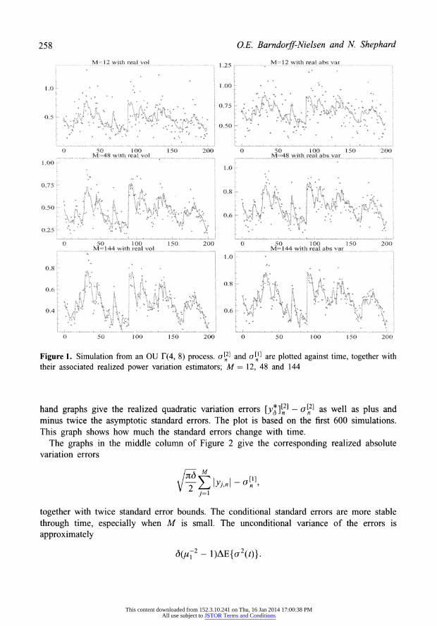
where z is a subordinator (cf. Examples 1 and 2 above). These models have been developed in this context by Barndorff-Nielsen and Shephard (2001). On the left in Figure 1 we have drawn curves to represent a simulated sample path of a[21 from an OU process where z(t) has a F(t4, 8) marginal distribution, A -log(0.99) and A= 1, along with the associated realized quadratic variation (depicted using crosses) computed using a variety of values of M. It is helpful to keep in mind that

1 1 1 E(u2(t)) = E(z(1)) - and var(a2(t)) - var(z(1)) - 2 2 32

The corresponding results for an]

and realized absolute variation are given on the right in Figure 1. We see that as M increases the precision of realized power variation increases, while Figure 1 shows that the variance of the realized power variation increases with the level of volatility. This is line with the prediction from the asymptotic theory, for the denominator increases with the level of volatility.

6.2.2. Quantile-quantile plots

To assess the finite-sample performance of the asymptotic distributions of the realized quadratic and absolute variation we have constructed some quantile-quantile (QQ) plots based upon the standardized errors (7) and (8). Our main focus will be on the absolute variation case, leaving the quadratic case to be covered in detail in a follow up paper by Barndorff-Nielsen and Shephard (2003). However, to start off with we give both cases, in order to enable an easy comparison.

Figure 2 gives QQ plots based on the simulation experiment reported in the previous subsection, with a sample size of 10000. Again we vary M over 12, 48 and 144. The left-




MN=48 wit rel vo M148 12with real abs var

01.00

0 0 M - 00 150 200 ) 50 00 oo :0 2oo

110

0077

00.50

0 0

0 50 100 150 200 0 50 10 O150 200 0.

0000

0 50 100 150 200 0 0 100 150 200

Figure 1. Simulation from an OU F(4, 8) process. ao2 and oa] are plotted against time, together with their associated realized power variation estimators; M= 12, 48 and 144

hand graphs give the realized quadratic variation errors [y-]n2] -an2

as well as plus and minus twice the asymptotic standard errors. The plot is based on the first 600 simulations. This graph shows how much the standard errors change with time.

The graphs in the middle column of Figure 2 give the corresponding realized absolute variation errors

12 yj, nl - Un

j= 1

together with twice standard error bounds. The conditional standard errors are more stable through time, especially when M is small. The unconditional variance of the errors is approximately

6(u12

- 1)AE{u2(t)}.




M 1 ...b ....th r.. ab v..

0 25( 500 0 250 500 -,2.5 00 25

050

0 0.205

(to

...... ....... ....5 0 2 0

500. 0 250 500 .. 5 0 0

5O

Ooc0 0.3 -2

M-4_25 M

-0.20 0

0(5(00o0) -25 0. 2-

Figure 2. Plots of the realized quadratic variation error and the realized absolute variation error plus twice their asymptotic standard errors; M= 12, 48 and 144. Corresponding QQ plots are on the right, based on the standardized realized quadratic variations and the realized absolute variations

The right-hand side of Figure 2 gives the associated QQ plots for the standardized residuals from the realized quadratic and absolute variation measures. These use all 10000 observations. The results are clear: in comparison with the asymptotic limit laws both random variables are too fat-tailed in small samples, with this problem reducing as M increases. The realized absolute variation version of the statistic has much better finite- sample behaviour, while the realized quadratic variation is quite poorly behaved.

6.2.3. Logarithmic transformation

The realized power variation [y*][r](t) is the sum of non-negative items and so is non- negative. It would seem sensible to transform this variable to the real line in order to improve its finite-sample performance. Hence we use the standard logarithmic transformation, that is, for a consistent estimator 0 of 0 we approximate log(0) by log(0) + (0 - 0)/0,




hence the asymptotic distribution of 0 - 0 can be used to deduce the asymptotic distribution of log(0) - log(0). For the general realized power variation this implies

%t

log[y7l6l-r/2[y*][r](t)] - log ar(s)ds o 60 N(0, 1). (27)

Pr 161-r/2

(r 2r)( ][2r](t)[y

-1r61-r/2[y r][(2)

Referring to the denominator, we should note that

t

,-rl 1-r[~[2r] a2r(s)ds -+> 1,

[/-I61-r/2[y*][r](t)]2 t 2 , r 6f o ar(s)d s

by Jensen's inequality. In the realized absolute variation case, (27) simplifies to

M t log{ V/(-6/2) 3

y.(t) } - log J(s)ds

j=l1 0 01- N(0, 1). (28) M M

6(7/2 - 1)( y(t))/{ |/2 • (t) }2 j=1 j=1

Using the same simulation set-up as employed in the previous subsection, we plot in Figure 3 the log version of the realized absolute variation error

log E yj,n| 109lOF[']l C2 j= I1

plus and minus twice the corresponding standard errors using (28). The standard errors have now stabilized, almost not moving with n. This is not surprising for t times

t

tv' Ju2(s)ds t-1 o a 2(s)ds

is empirically very close to one for small values of t, while for large t it converges to

E{u2(t)}

[E{or(t)}]2'

so long as the volatility process is ergodic and the moments exist. The corresponding QQ plots in Figure 3 have also improved, with the normality

approximation being accurate even for moderate values of M. This result carries over to wider simulations we have conducted.




12 th 1 abs

.. ... . ....... . M

.(,,).g irhe a l a

f, . ... ..... ........ .. ................. . . .. ... ..... 21

.................... .... 005

0 10o0 200 300 400 500 600 -3

2- 0 2

No4 ,o oi b ~ h ,) f c a .............

. .......... .... .. ..... ....... ....... .. .............. ... .....

. 0-2,5 2 ide e

0 1 o0 200 300 400 500 600 ..3 . 1 02 M 144i th w

0A

0.

2

0 100 200 300 400 500 60 AJO - 0 I 2 3

Figure 3. Plots of the log transform of the realized absolute variation. Left-hand plots are the errors plus and minus twice their asymptotic standard errors. Corresponding QQ plots are on the right, based on the standardized log realized absolute variations

Barndorff-Nielsen and Shephard (2003) have studied the effect of taking log transforms in the case of r = 2. That paper used simulation and some theory to show the beneficial effect of taking a log and comparing its effectiveness with other transformations.

7. Conclusions

This paper has introduced the idea of realized power variation, which generalizes the concept of realized volatility. The asymptotic analysis we provide, for 6 t 0, represents a significant extension of the usual quadratic variation result. Further, we provide a limiting distribution theory which considerably strengthens the consistency result and allows us to understand the variability of the difference between the realized power variation and the actual power volatility.




We have seen that when we take a log transformation of the realized power variation, the finite-sample performance of the asymptotic approximation to the distribution of this estimator improves and seems to be accurate even for moderate values of M.

Our motivation for the study reported in this paper came originally from mathematical finance and financial econometrics, where volatility is a key object of study. However, stochastic models in the form of a 'signal' a* plus a noise term e, where e is (conditionally) Gaussian with a variance that varies from 'site' to 'site', are ubiquitous in the natural and technical sciences, and we believe that results similar to those discussed here will be of interest for applications in a variety of other fields, for instance in turbulence and in spatial statistics (in this connection, see Guyon and Leon 1989).

Finally, the thesis of Becker (1998) consists of a comprehensive study of the limit behaviour as M

-- oc of processes of the type

y Imt)- UjM' /M - j= 1

X X M

where f is function of two variables and x denotes a Brownian semimartingale (of a certain kind; see below). The diffusion case is especially important. Extensions to general continuous or purely discontinuous semimartingales and even combination of the two are presented. The thesis is partly based on an earlier report by Jacod (1993; see also Delattre and Jacod (1997) and Florens-Zmirou (1993). Both x and f may be multidimensional, and generalizations to cases where not only the increment of x over the jth interval but also the whole trajectory over that interval occurs in the second argument of f are also considered.

We shall not attempt to indicate here the precise results and the accompanying regularity conditions of Becker's thesis in any detail, but we wish to underline that the setting of his study is extremely general. Of immediate interest in connection with the present paper are his results when x is a Brownian semimartingale. More specifically, Becker considers the case x where of the form

t it

x(t) - c(s)ds + o(s)dw(s),

where w is Brownian motion and c and a are predictible and subject to restrictions on their variational behaviour. He shows, in particular, that yM(t) converges, after suitable centring, to a stochastic process which is representable as a certain type of stochastic integral where the integration is with respect to a 'martingale-measure tangential to x'. A key point of our present work is that for the kind of functions f we consider (absolute powers), we are able to identify the limit behaviour as mixed Gaussian and, crucially for statistical applicability, from this to establish standard normal limit statements using random rescaling by observable scale factors.

Acknowledgements

This paper represents a revision of the paper 'Higher order variation and stochastic volatility models', which first appeared on 4 July 2001. It had the result that (25) converges




to zero when r = 2, 4, 6, ... The general asymptotic distribution result contained in (6)

was first discussed in public on 11 August 2001 at the Market Microstructure Conference, Centre for Analytical Finance, Denmark. Comments by Tim Bollerslev, Svend Erik Graversen, Matthias Winkel and the referees have been very helpful.

Ole E. Barndorff-Nielsen's work is supported by the Centre for Analytical Finance

(www.caf.dk), which is funded by the Danish Social Science Research Council, and by the Centre for Mathematical Physics and Stochastics (www.maphysto.dk), which is funded by the Danish National Research Foundation. Neil Shephard's research is supported by the UK Economic and Social Research Council through the grant 'Econometrics of trade-by-trade price dynamics', which is coded R00023839.

References

Andersen, T.G. and Bollerslev, T. (1997) Intraday periodicity and volatility persistence in financial markets. J Empir. Finance, 4, 115-158.

Andersen, T.G. and Bollerslev, T. (1998a) Answering the skeptics: yes, standard volatility models do provide accurate forecasts. Internat. Econom. Rev., 39, 885-905.

Andersen, T.G. and Bollerslev, T. (1998b) Deutsche mark-dollar volatility: intraday activity patterns, macroeconomic announcements, and longer run dependencies. J Finance, 53, 219-265.

Andersen, T.G., Bollerslev, T., Diebold, EX. and Ebens, H. (2001a) The distribution of realized stock return volatility. J Financial Econom., 61, 43-76.

Andersen, T.G., Bollerslev, T., Diebold, EX. and Labys, P. (2001b) The distribution of exchange rate volatility. J Amer Statist. Assoc., 96, 42-55.

Andreou, E. and Ghysels, E. (2002) Rolling-sampling volatility estimators: some new theoretical, simulation and empirical results. J Business Econom. Statist., 20, 363-376.

Areal, N.M.P.C. and Taylor, S.J. (2002) The realized volatility of FTSE-100 futures prices. J Futures Markets, 22, 627-648.

Bai, X., Russell, J.R. and Tiao, G.C. (2000) Beyond Merton's utopia: effects of non-normality and dependence on the precision of variance estimates using high-frequency financial data. Unpublished paper, Graduate School of Business, University of Chicago.

Barndorff-Nielsen, O.E. and Shephard, N. (2001) Non-Gaussian Ornstein-Uhlenbeck-based models and some of their uses in financial economics (with discussion). J Roy. Statist. Soc. Ser. B, 63, 167-241.

Barndorff-Nielsen, O.E. and Shephard, N. (2002) Econometric analysis of realized volatility and its use in estimating stochastic volatility models. J Roy. Statist. Soc. Ser. B, 64, 253-280.

Barndorff-Nielsen, O.E. and Shephard, N. (2003) How accurate is the asymptotic approximation to the distribution of realized volatility? In D. Andrews, J. Powell, PA. Ruud, and J.H. Stock (eds), Identification and Inference for Econometric Models. A Festschrifit in Honour of Thomas J Rothenberg, Econometric Society Monograph Series. Cambridge: Cambridge University Press. Forthcoming.

Becker, E. (1998) Theoremes limites pour des processus discretise's. Doctoral thesis, Universite Paris 6.

Bollerslev, T. and Forsberg, L. (2002) Bridging the gap between the distribution of realized ECU volatility and ARCH modelling of the Euro: The GARCH normal inverse Gaussian model. J Appl. Econometrics, 17, 535-548.




Bollerslev, T. and Zhou H. (2002) Estimating stochastic volatility diffusion using conditional moments of integrated volatility. J Econometrics, 109, 33-65.

Cao, C.Q. and Tsay, R.S. (1992) Nonlinear time-series analysis of stock volatilities. J Appl. Econometrics, 7, S165-S185.

Christensen, B.J. and Prabhala, N.R. (1998) The relation between implied and realized volatility. J Financial Econom., 37, 125-150.

Corsi, F., Zumbach, G., Miller, U. and Dacorogna, M. (2001) Consistent high-precision volatility from high-frequency data. Unpublished paper, Olsen and Associates, Zurich.

Dacorogna, M.M., Miller, U.A., Olsen, R.B. and Pictet, O.V (1998) Modelling short term volatility with GARCH and HARCH. In C. Dunis and B. Zhou (eds), Nonlinear Modelling of High Frequency Financial Time Series. Chichester: Wiley.

Davis, R.A. and Mikosch, T. (1998) The limit theory for the sample ACF of stationary process with heavy tails with applications to ARCH. Annals of Statistics, 26, 2049-2080.

Delattre, S. and Jacod, J. (1997) A central limit theorem for normalized functions of the increments of a diffusion process, in the presence of round-off errors. Bernoulli, 3, 1-28.

Ding, Z., Granger, C.W.J. and Engle, R.F. (1993) A long memory property of stock market returns and a new model. J Empir. Finance, 1, 83-106.

Florens-Zmirou, D. (1993) On estimating the diffusion coefficient from discrete observations. J Appl. Probab., 30, 790-804.

Galbraith, J.W. and Zinde-Walsh, V (2000) Properties of estimates of daily GARCH parameters based on intra-day observations. Unpublished paper, Economics Department, McGill University.

Ghysels, E., Harvey, A.C. and Renault, E. (1996) Stochastic volatility. In C.R. Rao and G.S. Maddala (eds), Statistical Methods in Finance, pp. 119-191. Amsterdam: North-Holland.

Granger, C.W.J. and Ding, Z. (1995) Some properties of absolute returns, an alternative measure of risk. Ann. Econom. Statist., 40, 67-91.

Granger, C.W.J. and Sin, C.-Y. (2002) Modelling the absolute returns of different stock indices: exploring the forecastability of an alternative measure of risk. J Forecasting. Forthcoming.

Guyon, X. and Leon, J. (1989) Convergence en loi des H-variations d'un processus gaussien stationnaire sur R. Ann. Inst. H. Poincare Probab. Statist., 25, 265-282.

Heston, S.L. (1993) A closed-form solution for options with stochastic volatility, with applications to bond and currency options. Rev. Financial Stud., 6, 327-343.

Hull, J. and White, A. (1987) The pricing of options on assets with stochastic volatilities. J Finance, 42, 281-300.

Jacod, J. (1993) Limit of random measures associated with the increments of a Brownian semimartingale. Preprint, Paris 6.

Jorion, P. (1995) Predicting volatility in the foreign exchange market. J. Finance, 50, 507-528.

Lyons, T. (1994) Differential equations driven by rough signals. I. An extension of an inequality by L.C. Young. Math. Res. Lett., 1, 451-464.

Maheswaran, S. and Sims, C.A. (1993) Empirical implications of arbitrage-free asset markets. In P.C.B. Phillips (ed.), Models, Methods and Applications of Econometrics. Cambridge, MA: Basil Blackwell.

Maheu, J.M. and McCurdy, T.H. (2002) Nonlinear features of realised FX volatility. Rev. Econom. Statist., 84, 668-681.

Meddahi, N. and Renault, E. (2002) Temporal aggregation of volatility models. J Econometrics. Forthcoming.

Mikosch, T. and Norvai'a, R. (2000) Stochastic integral equations without probability. Bernoulli, 6, 401-434.




Mikosch, T. and Starica, C. (2000) Limit theory for the sample autocorrelations and extremes of a GARCH(1, 1) process. Ann. Statist., 28, 1427-1451.

Nicolato, E. and Venardos, E. (2002) Option pricing in stochastic volatility models of the Ornstein- Uhlenbeck type. Math. Finance. Forthcoming.

Poterba, J. and Summers, L. (1986) The persistence of volatility and stock market fluctuations. Amer. Econom. Rev., 76, 1124-1141.

Renault, E. (1997) Econometric models of option pricing errors. In D.M. Kreps and K.F. Wallis (eds), Advances in Economics and Econometrics: Theory and Applications, pp. 223-78. Cambridge: Cambridge University Press.

Schwert, G.W. (1989) Why does stock market volatility change over time? I Finance, 44, 1115-1153. Shiryaev, AN. (1999) Essentials of Stochastic Finance: Facts, Models and Theory. Singapore: World

Scientific. Taylor, S.J. (1986) Modelling Financial Time Series. Chichester: Wiley. Taylor, S.J. and Xu, X. (1997) The incremental volatility information in one million foreign exchange

quotations. J Empir. Finance, 4, 317-340. West, K.D. and Cho, D. (1995) The predictive ability of several models for exchange rate volatility. J

Econometrics, 69, 367-391.

Received October 2001 and revised July 2002



International Statistical Institute (ISI) and Bernoulli...

Documents

Transcript of International Statistical Institute (ISI) and Bernoulli...