International Journal of Multiphase Flow 90 (2017) 102–117

Contents lists available at ScienceDirect

International Journal of Multiphase Flow

journal homepage: www.elsevier.com/locate/ijmulflow

Multiscale tow-phase flow modeling of sheet and cloud cavitation

Chao-Tsung Hsiao

∗, Jingsen Ma , Georges L. Chahine

Dynaflow, Inc., 10621-J Iron Bridge Road, Jessup, MD, USA

a r t i c l e i n f o

Article history:

Received 20 July 2016

Revised 20 October 2016

Accepted 25 December 2016

Available online 5 January 2017

a b s t r a c t

A multiscale two-phase flow model based on a coupled Eulerian/Lagrangian approach is applied to cap-

ture the sheet cavitation formation, development, unsteady breakup, and bubble cloud shedding on a

hydrofoil. No assumptions are needed on mass transfer. Instead natural free field nuclei and solid bound-

ary nucleation are modelled and enable capture of the sheet and cloud dynamics. The multiscale model

includes a micro-scale model for tracking the bubbles, a macro-scale model for describing large cavity dy-

namics, and a transition scheme to bridge the micro and macro scales. With this multiscale model small

nuclei are seen to grow into large bubbles, which eventually merge to form a large scale sheet cavity. A

reentrant jet forms under the sheet cavity, travels upstream, and breaks the cavity, resulting in the emis-

sion of high pressure peaks as the broken pockets shrink and collapse while travelling downstream. The

method is validated on a 2D NACA0015 foil and is shown to be in good agreement with published exper-

imental measurements in terms of sheet cavity lengths and shedding frequencies. Sensitivity assessment

of the model parameters and 3D effects on the predicted major cavity dynamics are also discussed.

© 2017 Elsevier Ltd. All rights reserved.

s

w

o

t

m

h

t

H

t

t

i

i

f

i

1

fl

1

d

m

c

b

o

f

1. Introduction

Various types of cavitation occur over a propeller blade. These

include traveling bubble cavitation, tip vortex cavitation, sheet cav-

itation, cloud cavitation, supercavitation, and combinations of the

above. Among these, the transition from sheet to cloud cavitation

is recognized as the most erosive and is quite difficult to accurately

model. The sheet cavity starts near the leading edge, effectuates

large amplitude length/volume oscillations, and breaks up periodi-

cally releasing clouds of bubbles and cavitating vortical structures,

which collapse violently generating high local pressures on the

blade. Accurate simulation and modeling of the physics involved

is challenging since the problems of sheet cavity dynamics, cloud

cavity dynamics, and sheet-to-cloud transition involve length and

time scales of many different orders of magnitude.

Experimental observations have indicated weak or little de-

pendence of the sheet cavity inception and dynamics on the nu-

clei distribution in the test facility, which has led many numer-

ical modelers to believe that sheet cavitation is not connected

with bubble dynamics. Actually, over the years, several researchers

(e.g. Kodama et al., 1981 ; Kuiper, 2010 ) have observed that the

presence of free field nuclei affected significantly the repeata-

bility of the experimental results. In experiments where nuclei

count was very low the value of the incipient cavitation number

∗ Corresponding author.

E-mail addresses: ctsung@dynaflow-inc.com (C.-T. Hsiao), jingsen@dynaflow-

inc.com (J. Ma), glchahine@dynaflow-inc.com (G.L. Chahine).

(

S

S

b

http://dx.doi.org/10.1016/j.ijmultiphaseflow.2016.12.007

0301-9322/© 2017 Elsevier Ltd. All rights reserved.

howed large scatter, whereas in water rich in nuclei the results

ere more repeatable and were not affected by further addition

f nuclei. One potential explanation to the above observations is

hat nucleation from the solid surface of the blades could play a

uch more important role than the free field nuclei, and this may

ave been overlooked in previous studies of sheet cavitation even

hough bubble nucleation has been extensively investigated (e.g.

arvey et al., 1944 ; Yount, 1979; Mørch, 2009 ).

Conventional numerical approaches for modeling sheet cavi-

ies cannot address travelling bubble cavitation or sheet cavita-

ion inception. Instead, they assume that the cavity already exits,

s filled with vapor at the liquid vapor pressure and thus arbitrar-

ly define as a liquid-cavity interface the liquid iso-pressure sur-

ace with the vapor pressure value. The flow solution in the liquid

s obtained using either a Navier–Stokes solver ( Deshpande et al.,

993 ; Chen and Heister, 1994 ; Hirschi et al., 1998 ) or a potential

ow solver using a boundary element method ( Kinnas and Fine,

993 ; Chahine and Hsiao, 20 0 0 ; Varghese et al., 20 05 ). Since the

eveloped sheet cavity is very unsteady and dynamic, numerical

ethods requiring a moving grid to resolve the flow field are ac-

urate but encounter numerical difficulties to describe folding or

reaking up interfaces. Other approaches have thus been devel-

ped to avoid using moving grids to track the liquid-gas inter-

ace. They are mainly in two categories: Volume of Fluid methods

VoF) ( Merkle et al., 1998 ; Kunz et al., 20 0 0 ; Yuan et al., 2001 ;

inghal et al., 2002 ) and Level-Set Methods (LSM) ( Kawamura and

akoda, 2003 ; Dabiri et al., 2007 , 2008, Kinzel et al., 2009 ). While

oth interface capturing methods solve the Navier–Stokes equa-

C.-T. Hsiao et al. / International Journal of Multiphase Flow 90 (2017) 102–117 103

t

c

f

m

p

u

u

l

a

r

t

a

z

G

t

b

o

r

(

i

o

q

l

a

2

c

c

m

v

s

a

c

b

C

S

c

(

g

a

m

2

b

H

a

m

b

t

c

m

b

C

h

t

s

c

w

w

t

s

p

t

a

e

j

i

o

v

n

E

b

2

m

p

a

p

c

t

t

f

C

b

c

2

s

n

ρ

w

m

T

p

ρ

w

t

ions using a fixed computational grid, the liquid/gas interface is

aptured differently. In the VoF method, an advection equation

or the volume fraction of the vapor is solved and the two-phase

edium density is computed knowing the volume fraction of each

hase. This method applies a mass transfer model between the liq-

id and the cavity to model liquid/vapor exchange at the interface

sing ‘calibration’ parameters to match experimental results. In the

evel set method, the interface location is determined by solving

n advection equation for the level set function with the interface

epresented by the zero level (or iso-surface) of the level-set func-

ion. In this method boundary conditions similar to those used in

n interface tracking scheme (e.g. a constant pressure value and

ero shear stress) can be imposed at the zero level set surface if a

host Fluid Method is used ( Fedkiw et al., 1999 ).

Interface capturing approaches have been successfully applied

o describe the dynamic evolution of a cavitation sheet and its

reakup but not to the dispersed bubble phase and to the res-

lution of the transition from sheet to bubbles since this would

equire an extremely fine spatial resolution relative to bubble size

Fedkiw et al., 1999 ; Osher and Fedkiw, 2001 ). Resolving sheet cav-

ty together with the microbubbles involves characteristic lengths

f different orders of magnitude and using the smallest scale re-

uires computational resources not currently available.

Instead of resolving all individual bubbles, continuum-based Eu-

erian approaches ( Biesheuvel and Van Wijngaarden, 1984 ; Zhang

nd Prosperetti, 1994a,b ; Druzhinin and Elghobashi, 1998, 1999,

001 ; Ma et al., 2011, 2012 ) assuming the bubbly phase to be a

ontinuum are typically used for bubbles much smaller than the

haracteristic lengths associated with the motion of the overall

ixture. In this case, the precise location and properties of indi-

idual bubbles are not directly apparent at the global mixture flow

cale. As a result, this approach is not able to address appropri-

tely the bubble dynamics and interactions which are important in

avitation and more so in cloud cavitation.

Approaches combining both continuum and discrete bub-

les have been proposed ( Chahine and Duraiswami, 1992 ;

hahine, 2009 ; Balachandar and Eaton, 2010 ; Raju et al., 2011 ;

hams et al., 2011 ; Hsiao et al., 2013 ). In these approaches the

arrier fluid is modeled using standard continuum fluid methods

Eulerian approach) and dispersed bubbles are tracked directly (La-

rangian approach). The interaction between the two phases is

chieved through a locally distributed force field imposed in the

omentum equation ( Ferrante and Elghobashi, 2004 ; Xu et al.,

002 ) or through the inclusion of local density variation due to

ubble motion and dynamics ( Chahine, 2009 ; Raju et al., 2011 ;

siao et al., 2013 ; Ma et al., 2015a ).

We have recently developed a multiscale method, which aims

t addressing all the various scales of the problem; notably a

acro-scale at the order of the blade length, a micro-scale for the

ubble nuclei, an intermediary scale for the bubble clouds, and

ransition and coupling procedures between these scales. To in-

lude sheet cavitation inception in the study, we use the same

odel and code that we have pioneered to study travelling bub-

le or tip vortex cavitation inception ( Chahine, 2004 ; Hsiao and

hahine, 2004 ; Hsiao and Chahine, 20 08 ; Chahine, 20 09 ) and en-

ance it to include a two-phase medium as well as large cavi-

ies. This starts from the precept that water always contains micro-

copic bubble nuclei and solid liquid interfaces do not have perfect

ontact and thus entrap nanoscopic or microscopic gas pockets,

hich are a source of nucleation (freeing of nuclei into the liquid)

hen appropriate local conditions occur. Cavitation inception of all

ypes is initiated through explosive growth of these nuclei. With

uch nucleation models, the multiscale two-phase flow model, as

resented in this paper, not only can simulate the sheet cavita-

ion accurately without the assumption of mass transfer, it can

lso allow us to simulate different nuclei conditions which may be

ncountered in different experimental applications. Another ma-

or advantage of the current multiscale two-phase flow model is

ts use of an Eulerian-Lagrangian coupled approach, which allows

ne to account for the unresolved phase. While most of the pre-

ious studies have investigated statistically averaged dynamics ig-

oring the slip velocity between the bubble and liquid phases, the

ulerian–Lagrangian approach is also able to include slip velocity

etween phases, which can be large and is essential for accuracy.

. Numerical model

The sketch in Fig. 1 presents an overview of the multiscale

odel developed in this study. This model aims at addressing the

hysics at the various scales involved in sheet and cloud cavitation:

• At the micro-scale, transport of nuclei and microbubbles, nucle-

ation from solid surfaces, and corresponding bubble dynamics

are considered. The model addresses dispersed pre-existing nu-

clei in the liquid, nuclei originating from solid boundaries, and

micro-bubbles resulting from disintegration of sheet and cloud

cavities or bubbles breaking up from vaporous/gaseous cavities.

At this scale, the model tracks the bubbles in a Lagrangian fash-

ion. • At the macro-scale, a two-phase continuum-based flow is

solved on an Eulerian grid. At this scale gas/liquid interfaces of

large bubbles, air pockets, and cavities are directly discretized

and resolved through tracking the gas-liquid interfaces with a

Level Set method. • Inter-scale transition schemes are used to bridge micro and

macro scales as bubbles grow or merge to form large cavi-

ties, or as bubbles shrink or break up from a large cavity. At

this scale, model transition between micro-scale and macro-

scale and vice-versa is realized by using information from both

the Discrete Singularity Model (DSM) and the Level Set method

(LSM).

To handle the interaction between the unresolved bubbles

nd the two-phase medium, a coupled Eulerian/Lagrangian two-

hase flow model is used. The Eulerian approach addresses the

ontinuum-based two-phase model while the Lagrangian approach

racks sub-grid bubble motion and dynamics. This method was ini-

ially developed to simulate directly cavitation inception and noise

or traveling and tip vortex cavitation ( Chahine, 2004 ; Hsiao and

hahine, 2004 ; Hsiao and Chahine, 2008 ), bubble dynamics in a

ubbly medium ( Raju et al., 2011 ; Ma et al., 2015a ), and bubble

loud dynamics ( Ma et al., 2015b ).

.1. Eulerian continuum-based two-phase model

The two-phase medium continuum model uses a viscous flow

olver to solve the Navier–Stokes equations and satisfy the conti-

uity and momentum equations:

∂ ρm

∂t + ∇ · ( ρm

u ) = 0 , (1)

m

D u Dt

= −∇ p + ∇

{τi j − 2

3 μm

( ∇ · u ) δi j

},

τi j = μm

(∂ u i ∂ x j

+

∂ u j ∂ x i

),

(2)

here the subscript m refers to the mixture properties. u is the

ixture velocity, p is the pressure, and δij is the Kronecker delta.

he mixture density, ρm

, and the mixture viscosity, μm

, can be ex-

ressed as functions of the void volume fraction α:

m

= ( 1 − α) ρl + αρg , μm

= ( 1 − α) μl + αμg , (3)

here the subscript l refers to the liquid and the subscript g refers

o the gas.

104 C.-T. Hsiao et al. / International Journal of Multiphase Flow 90 (2017) 102–117

Fig. 1. Overview of the various scales involved in the problem of cavitation on a foil and sketch of the modeling strategy.

d

v

o

t

u

a

o

l

b

t

2

s

c

(

ϕ

w

d

d

ϕ

s

w

e

i

f

n

e

w

S

i

p

o

The equivalent medium has a time and space dependent den-

sity since the void fraction α varies in both space and time. This

makes the overall flow field problem similar to a compressible flow

problem, but wave phenomena such as shocks emitted by collaps-

ing bubble will not be accurately predicted as the present approach

is not aiming for such flow details. In our approach, which cou-

ples the continuum medium with the discrete bubbles, the mix-

ture density is not an explicit function of the pressure through an

equation of state. Instead, tracking the bubbles and knowing their

concentration provides α and ρm

as functions of space and time.

This is achieved by using a Gaussian distribution scheme which

smoothly “spreads” each bubble’s volume over neighboring cells

within a selected radial distance while conserving the total bubble

volumes ( Ma et al., 2015a ). Specifically, in a fluid cell i , the void

fraction is computed using:

αi =

N i ∑

j=1

f i, j V

b j ∑ N cel l s

k f k, j V

cell k

, (4)

where V b j and V cell

k are the volumes of a bubble j and cell k re-

spectively, N i is the number of bubbles which are influencing cell

i . N cells is the total number of cells “influenced” by a bubble j. f i,j is the weight of the contribution of bubble j to cell i and is deter-

mined by the Gaussian distribution function. This scheme has been

found to significantly increase numerical stability and to enable the

handling of high-void bubbly flow simulations.

The system of equations is closed by an artificial compressibil-

ity method ( Chorin, 1967 ) in which a pseudo-time derivative of

the pressure multiplied by an artificial-compressibility factor, β , is

added to the continuity equation as

1

β

∂ p

∂τ+

∂ ρm

∂t + ∇ · ( ρm

u ) = 0 . (5)

As a consequence, a hyperbolic system of equations is formed

and can be solved using a time marching scheme. This method

can be marched in pseudo-time to reach a steady-state solution.

To obtain a time-dependent solution, a Newton iterative procedure

is performed at each physical time step in order to satisfy the con-

tinuity equation. It is noted that using the artificial compressibil-

ity method alters the speed of sound and thus enables to use the

scheme in the low Mach number regime such as the current prob-

lem for the flow over a hydrofoil.

The Navier–Stokes solver uses a finite volume formulation.

First-order Euler implicit differencing is applied to the time deriva-

tives. The spatial differencing of the convective terms uses the flux-

ifference splitting scheme based on Roe’s method ( Roe, 1981 ) and

an Leer’s MUSCL method ( van Leer, 1979 ) for obtaining the first-

rder and the third-order fluxes, respectively. A second-order cen-

ral differencing is used for the viscous terms which are simplified

sing the thin-layer approximation. The flux Jacobians required in

n implicit scheme are obtained numerically. The resulting system

f algebraic equations is solved using the Discretized Newton Re-

axation method ( Vanden and Whitfield, 1995 ) in which symmetric

lock Gauss–Seidel sub-iterations are performed before the solu-

ion is updated at each Newton iteration.

.2. Level-set approach

In order to enable the multiscale code to simulate large free

urface deformations such as folding and breakup in the sheet

avity problem, a Level-Set method using the Ghost Fluid Method

Fedkiw et al., 1999 ; Kang et al., 20 0 0 ) is used. A smooth function

( x,y,z,t ), whose zero level coincides with the liquid/gas interface

hen the level set is introduced, is defined in the whole physical

omain (i.e. in both liquid and gas phases) as the signed distance

( x,y,z ) from the interface:

( x, y, z, 0 ) = d ( x, y, z ) . (6)

This function is enforced to be a material surface at each time

tep using:

dϕ

dt =

∂ϕ

∂t + u ∇ϕ = 0 , (7)

here u is the velocity of interface. Integration of Eq. (7) does not

nsure that the thickness of the interface region remains constant

n space and time during the computations due to numerical dif-

usion and to distortion by the flow field. To avoid this problem, a

ew distance function is constructed by solving a “re-initialization

quation” in pseudo time iterations ( Sussman, 1998 ):

∂ϕ

∂τ= S ( ϕ 0 ) [ 1 − | ∇ϕ | ] , (8)

here τ is the pseudo time, ϕ0 is the initial distribution of ϕ, and

( ϕ0 ) is a sign function, which is zero at the interface.

Eqs. (7) and (8) are solved with a Ghost Fluid Method impos-

ng boundary conditions at the interface after identifying to which

hase a concerned cell belongs. Fig. 2 illustrates the identification

f the cells. When one of the following six inequalities is satisfied

C.-T. Hsiao et al. / International Journal of Multiphase Flow 90 (2017) 102–117 105

Fig. 2. Cell location identification in the computational domain.

f

ϕ

ϕ

ϕ

t

a

t

a

w

w

i

κ

i

t

t

t

c

l

t

E

a

t

n

w

d

v

d

e

2

i

g

d

(

2

m

p

2

c

t

ρ

w

t

b

t

p

t

W

t

m

w

g

t

T

t

t

f

2

t

s

t

R

w

g

T

z

a

c

n

l

b

f

ϕ

w

s

“

or two adjacent cells:

i, j,k ϕ i ±1 , j,k < 0 ,

i, j,k ϕ i, j±1 ,k < 0 ,

i, j,k ϕ i, j,k ±1 < 0 ,

(9)

he zero level-set interface is identified.

In this approach two ghost cells are used to impose the bound-

ry conditions at the interface cells without use of smoothing func-

ions. If the shear due to the air is neglected, the dynamic bound-

ry conditions (balance of normal stresses and zero shear) can be

ritten:

p =

n � τ � n

ρl

+

gz

ρl

+

γ κ

ρl

, n � τ � t = 0 , (10)

here τ is the stress tensor, g is the acceleration of gravity, and γs the surface tension.

=

∇ �∇ϕ

| ∇ϕ | (11)

s the surface curvature. n and t are the surface normal and tangen-

ial vectors, respectively.

Although the Ghost Fluid Method can help maintain a sharp in-

erface, additional computational cost is required for the cells in

he ignored phase, e.g. air. To further reduce the computational

ost we apply a single-phase level-set approach in which only the

iquid phase of the fluid is solved, while the cells belonging to

he gas phase are deactivated during the computations. To solve

q. (7) we use the velocity information from the gas cells which

re near the interface. To obtain this information, we assume that

he following condition across the interface applies:

�∇u = 0 , with n = ∇ϕ / |∇ϕ | , (12)

hich means there is no normal component of the velocity gra-

ient at the interface. With this assumption we can extend the

elocity from the liquid phase along the normal direction of the

istance function to the gas phase by solving the pseudo time it-

ration equation:

∂u

∂τ+ n �∇u = 0 . (13)

.3. Lagrangian discrete bubble model

The Lagrangian discrete bubble model, which enables tracking

nitially sub-grid nuclei in the flow, identifying when explosive

rowth (inception) and collapse (erosion) occur, is based on the

iscrete singularity model which uses a Surface Average Pressure

SAP) approach ( Hsiao et al., 20 03 ; Chahine, 20 04 ; Choi et al.,

004 ) to average fluid quantities along the bubble surface. This

odel has been shown to produce accurate results when com-

ared to full 3D two-way interaction computations ( Hsiao et al.,

003 ). The averaging scheme allows one to consider only a spheri-

al equivalent bubble and use a modified Rayleigh-Plesset equation

o describe the bubble dynamics,

l

(R ̈R +

3

2

˙ R

2 )

= p v + p g0

(R 0

R

)3 k

− p enc − 2 γ

R

− 4 μ ˙ R

R

+ ρl

| u s | 2 4

,

(14)

here the slip velocity, u s = u enc − u b , is the difference between

he encountered (SAP averaged) liquid velocity, u enc , and the bub-

le translation velocity, u b . R and R 0 are the bubble radii and time

and 0, p v is the liquid vapor pressure, p g0 is the initial bubble gas

ressure, k is the gas polytropic compression constant, and p enc is

he average SAP pressure “seen” by the bubble during its travel.

ith the SAP model, u enc and p enc are respectively the averages of

he liquid velocities and pressures over the bubble surface.

The bubble trajectory is obtained from the following bubble

otion equation:

d u b

dt =

(ρl

ρb

)[3

8 R

C D | u s | u s +

1

2

(d u enc

dt − d u b

dt

)

+

3 ̇

R

2 R

u s − ∇p

ρl

+

( ρb − ρl )

ρl

g +

3 C L 4 π

√

ν

R

u s × √ | |

]

, (15)

here ρb is the density of the bubble, C D is the drag coefficient

iven by an empirical equation, e.g. from Haberman and Mor-

on (1953) , C L is the lift coefficient and is the vorticity vector.

he first right hand side term is a drag force. The second and third

erms account for the added mass. The fourth term accounts for

he presence of a pressure gradient, while the fifth term accounts

or gravity and the sixth term is a lift force ( Saffman 1965 ).

.4. Transition model between micro- and macro-scale

The transition between micro- and macro-scale models includes

wo scenarios:

a. transition from collected coalescing microbubbles into relatively

large two-phase cavities,

b. transition from a large cavity into a set of micro-scale dispersed

bubbles.

In the first scenario a criterion based on bubble / cell relative

ize is set to “activate” bubbles for computation of a level set func-

ion:

≥ max ( R thr , m thr �L ) , (16)

here R thr is a threshold bubble radius, �L is the size of the local

rid which hosts the bubble, and m thr is a threshold grid factor.

herefore a bubble interface is activated and is represented by the

ero level set when the bubble radius exceeds a threshold value

nd becomes larger than a multiple of the local grid size.

At the beginning of the simulation where no cavity exists, all

ells have the same level set value, ϕLS 0 , fixed to be a very large

egative value. When bubbles are detected to satisfy Eq. (16) , the

evel set value of each cell in the computation domain is modified

ased on the distance from each cell center to the bubbles’ sur-

aces, using the following equation:

i = min ( ϕ LS0 , ϕ b, j ) ; j = 1 , N i , (17)

here ϕb, j is the local distance function computed based on the

urface of bubble j , and N i is the number of bubbles which are

activated” around cell i .

106 C.-T. Hsiao et al. / International Journal of Multiphase Flow 90 (2017) 102–117

f

d

t

l

N

t

c

d

s

p

t

w

t

3

3

N

v

t

w

a

g

s

d

3

g

f

d

a

s

b

r

b

c

o

f

a

b

a

T

t

5

s

p

1

t

2

(

c

l

t

v

This scheme allows multiple bubbles to merge together into a

large cavity, or isolated bubbles to coalesce with a previously de-

fined large cavity.

In the second scenario, we use the zero level-set to identify

the gas/liquid interface of the cavity. The volume of the cavity is

tracked at each time step to determine when the cavity collapse

occurs. As the cavity collapses, surface instabilities and cavity dis-

integration are accounted for using empirical criteria based on ex-

perimental observations such as described in Ma et al. (2011) and

Hsiao et al. (2013) . The model assumes that turbulence at the free

surface produces a rough gas/liquid interface, which consists of a

bubbly layer with microbubbles of size, a . These cavities will be

entrained into the liquid once the local downward liquid velocity

of this mixture layer, u n ( a /2), exceeds the mean downward veloc-

ity of the free surface, u n (0). An amount of micro-bubbles of the

same volume is initiated around the cavity to replace volume loss

between time steps. The procedure is similar to that used to simu-

late bubble entrainment in breaking waves. Micro-bubbles are en-

trained into the liquid once the local normal velocity pointing to-

wards the liquid exceeds the speed of the gas/liquid interface. This

leads to a simple expression for the location and rate of bubble

generation that is proportional to the liquid’s local turbulent ki-

netic energy times the gradient of the liquid velocity in the liquid

normal direction.

2.5. Nucleation model

The simulations presented below use free field nuclei as mea-

sured experimentally by many researchers such as Medwin (1977) ,

Billet (1985) , Franklin (1992) and Wu et al. (2010) . In our modeling

the bubbles are distributed randomly in the liquid following the

measured bubble size distribution, as more detailed in our previ-

ous work in Chahine (20 04, 20 09) and Hsiao et al. (2013) . Another

important source of nuclei for the present problem is nuclei peri-

odically released from the foil surface. Boundary nucleation is eas-

ily observed in conditions where gas diffusion (beer or champagne

glass) and/or boiling are dominant; bubbles grow out of distributed

fixed spots. This phenomenon has been studied extensively in the

past. Harvey et al. (1944) suggested that gas pockets, trapped in

hydrophobic conical cracks and crevices of solid surfaces, act as

cavitation nuclei. More recently Mørch (2009) investigated this ef-

fect in more depth and suggested that a skin model similar to that

proposed by Yount (1979) for dispersed nuclei can also be used to

describe the wall gas bubbles because solid surfaces submerged in

a liquid tend to absorb amphiphilic molecules (molecules having a

polar water-soluble group attached to a nonpolar water-insoluble

hydrocarbon chain) and capture nanoscopic air pockets. One can

expect that clusters of such molecules form weak spots, which are

the source for bubble nucleation from the solid surface when low

pressure conditions are achieved. Briggs (2004) , for instance, found

that scrupulous cleaning was decisive for obtaining a high tensile

strength of water, and that contamination of interfaces is a primary

factor in cavitation. Atchley and Prosperetti (1989) modeled nucle-

ation out of crevices with liquid pressure drop. They identified un-

stable motion of the liquid-solid-gas contact line in the crevice and

unstable growth of the nucleus volume due to loss of mechani-

cal stability (force balance). Specifically, they related the threshold

pressure to crevice aperture, surface tension, and gas concentration

etc.

Based on existing experimental observations and theoretical

studies, the present work uses a nucleation model with the fol-

lowing characteristics parameters, which all are physical properties

characteristic of the foil material and should be deduced from im-

proved future characterization of material surfaces:

• P : a nucleation pressure threshold,

thr

• N s: a number density of nucleation sites per unit area, • f n: a nucleation time emission rate, function of the local flow

conditions, • R 0 : initial nuclei size, function of the local surface conditions .

In this nucleation model, at each time step, nuclei are released

rom the foil boundary cell when the pressure at the cell center

rops below a threshold value, P thr . The cell of surface area �A ,

hen releases N nuclei during the time interval �t , obtained as fol-

ows:

= N s f n �t�A. (18)

Since the Lagrangian solver (bubble tracking) usually requires

ime steps much smaller than the Eulerian flow solver, the N nuclei

an be released randomly in space from the area �A and in time

uring the Eulerian time step, �t .

It is expected that the above parameters are also functions of

urface roughness, S, temperature, T , and other physico-chemical

arameters not explicitly considered here. In this study, we use

his simplified nucleation model to investigate whether it enables

ith the above described overall multiscale approach to recover

he main characteristics of sheet cavitation.

. Sheet cavitation on a 2D hydrofoil

.1. Case setup

We study first the development of a sheet cavity over a 2D

ACA0015 hydrofoil to study the sensitivity of the solution to the

alues of the parameters used in the numerical model. An H–H

ype grid is generated with 181 × 101 grid points in the stream

ise and normal direction, respectively. Only 2 grid points are used

long the span wise direction to enforce two-dimensionality. 101

rid points are used on each side of the hydrofoil surface and non-

lip wall boundary conditions are imposed there. The grid is sub-

ivided into 12 blocks for a computational domain which extends

.0 chord-length upstream and 5.0 chord-length downstream. The

rid also extends 2.0 chord-length vertically away from the foil sur-

ace where far-field boundary conditions are applied. The grid is

esigned to provide high clustering around the hydrofoil surface

s shown in Fig. 3 . In particular, the first grid above the hydrofoil

urface is located within y + < 1 in order to properly capture the

oundary layer. The unsteady viscous flow field is simulated di-

ectly using the Navier–Stokes equations without applying any tur-

ulence modeling. Grid resolution was determined following grid

onvergence studies in previous work.

In this section, the foil is considered for the angles of attack

f 8 ° and 10 °. The chord length is 0.12 m, and the incoming flow

rom far-field upstream has a mean velocity of 10 m/s, resulting in

Reynolds number of 1.2 × 10 6 . The nuclei are dispersed in the

ulk of the liquid and are also released from the surface of the foil

ccording to the solid surface nucleation model described above.

he field nuclei are here selected to have radii ranging from 20 μm

o 60 μm, and correspond to an average initial void fraction of

.5 × 10 −5 .

Nucleation from the solid wall is initiated when the local pres-

ure drops below a critical value, here selected to be the vapor

ressure. The initial size of the nuclei emitted is selected to be

0 μm and the number of bubbles is determined by Eq. (18) with

he number of nucleation sites per unit area selected to be N s =24 /c m

2 and the nucleation frequency selected to be f n = 22 kHz

these choices are further discussed later). The microbubbles be-

ome a cavity described by a Level Set surface when they grow

arger than the size of the local grid and exceed 350 μm ( ∼10

imes the median initial nuclei size). The effects of these selected

alues of the parameters on the solution are investigated below.

C.-T. Hsiao et al. / International Journal of Multiphase Flow 90 (2017) 102–117 107

Fig. 3. Zoomed-in view of the multi-block grid used in this study for the simulation of sheet cavitation on a NACA0015 hydrofoil.

Fig. 4. Importance of the inclusion of wall nucleation on the proper modeling of

the sheet cavity using the Eulerian–Lagrangian and level set methods. Field nu-

clei alone do not reach the wall or grow enough to fill the cavity. σ = 1.65, α = 8 °, U ∞ = 10 m/s, L = 0.12 m, N s = 224 cm

−2 , F n = 22 kHz.

v

i

i

t

o

c

a

t

i

t

v

p

i

g

T

d

3

c

N

Fig. 5. Time sequence of sheet cavitation formation and cloud shedding with pres-

sure contours. ( σ = 1.65, α = 8 °, U ∞ = 10 m/s, L = 0.12 m). The white dots are discrete

bubbles and the white lines are the zero level-set lines denoting the liquid-vapor

interface.

Comparison of the numerical results with experimental obser-

ations are very satisfactory only when wall nucleation is taken

nto account, as described in more detail in the next section. This

s illustrated in Fig. 4 , which clearly shows a major difference be-

ween time average cavity sizes when wall nucleation is included

r when it is ignored. Accounting for field nuclei only is unable to

apture the sheet length properly unless the void fraction is rel-

tively high (above 10 −3 ). This is very much in agreement with

he experimental observations. Including the wall nucleation alone

s capable of capturing the sheet length but is insufficient to cap-

ure properly the events behind the cavity closure such as the de-

elopment of cloud cavities and cavitating vortical structures. This

rovide important insight into the physics of sheet cavities, imply-

ng that sheet inception and dynamics is mostly controlled by the

rowth and dynamics of nucleated bubbles from the foil surface.

his physics is in addition slightly effected by the presence and

ynamics of free field nuclei.

.2. Dynamics of the sheet cavity

A time sequence of sheet cavity shape oscillation and cloud

avitation shedding for one cycle is shown in Fig. 5 for σ = 1.65.

ucleation initiates at the hydrofoil surface near the leading edge

108 C.-T. Hsiao et al. / International Journal of Multiphase Flow 90 (2017) 102–117

Fig. 6. Zoom views of the velocity field and pressure contours around the sheet

cavity (Top) and a zoom view of the red-boxed region of the streamlines in the

reverse re-entrant jet flow region (Bottom).

Fig. 7. Time histories of the pressures and stream wise velocities at x = 0.4 L at the

solid wall near the sheet cavity trailing edge. σ = 1.65.

3

3

p

e

t

e

o

i

c

t

N

c

s

f

i

w

u

b

f

d

f

w

l

t

t

e

t

s

c

t

a

l

F

b

p

3

s

where the pressure drops below the selected nucleation threshold,

p thr = p v . Initially, bubble nuclei from the bulk of the liquid being

convected downstream, as well as nuclei released from the solid

surface, grow, coalesce and form a discrete small cavity described

with a level set function. Later, free field nuclei have difficulty to

enter in the cavity just move downward, while wall nucleation

keeps feeding vapor and gas into the sheet cavity which grows to

become a fully developed sheet cavity.

At the back of the cavity a stagnation flow forms ( Shen and Di-

motakis, 1989 ) as shown in the zoomed view in Fig. 6 . The reverse

flow results in a re-entrant jet, which moves upstream under the

sheet cavity and ultimately contributes to breaking the cavity into

two. The shed cavity collapses as it travels downstream generat-

ing high pressures. At the same time a new sheet cavity forms and

expands, and the cycle repeats.

This periodic shedding phenomenon can be further quantified

by analyzing the time histories of the instantaneous pressures and

stream wise velocities in the flow. For example, Fig. 7 shows the

pressures and velocities monitored at the first grid point in the liq-

uid on the suction side of the solid surface at the location x = 0.4 L

downstream of the leading edge. This is at about the same location

as the maximal extent of the trailing edge of the fully developed

sheet cavity. This location alternatively experiences positive and

negative stream-wise velocities with magnitudes as high as the in-

coming flow, U ∞

. The time interval between consecutive negative

velocity maxima is repeatable and has a value close to 1.15 L / U ∞

.

The corresponding oscillation frequency is about 0.86 U ∞

/ L , which

matches very well with the experimentally measured shedding fre-

quency for the same cavitation number ( Berntsen et al., 2001 ).

Fig. 7 also shows that each cycle of flow velocity oscilla-

tions coincides with the alternation of peaks and minimum pres-

sure values with the same oscillation frequency. This illustrates a

strong correlation between reentrant jet initiation and the develop-

ment of pressure fluctuations during each cycle of the sheet cavi-

tation.

.3. Sensitivity study of model parameters

.3.1. Nucleation model parameters

Since we do not have actual measured values of the nucleation

arameter, which we hope will become accessible in the future, we

xamine here the effects of the selection of the numerical values of

hese parameters on the simulation results. The nucleation param-

ters f n and N s , which express the number density and frequency

f the nuclei emitted from the wall, as expressed by Eq. (18) , are

nvestigated.

The left column of Fig. 8 compares the time-averaged sheet

avity shapes for different assumed nucleation rates, f n , and for

he same value of the number of nucleation sites per unit area,

s = 224 cm

−2 . The right column of Fig. 8 , on the other hand,

ompares the averaged shapes for different assumed nucleation

ites per unit area, N s , for the same value of the nucleation rate,

n = 22 kHz. The same information is shown in quantitative form

n Fig. 9 . It is seen that the time-averaged cavity length increases

ith the nucleation rate when f n is small, but then remains almost

nchanged for values of f n larger than 22 kHz. A similar trend can

e seen when N s is increased for a constant nucleation frequency,

n .

The time-averaged cavity length increases with the number

ensity N s when N s is small, but then remains almost unchanged

or values of N s larger than 112 cm

−2 . These trends imply that

hen the nucleation rate and nucleation sites per unit area are

arger than some values, the cavity length reaches a saturation sta-

us and shows negligible dependency on those parameters. Since

hese two parameters are associated with the solid surface prop-

rties, the implication of the results is that surface treatment of

he lifting surface can significantly influence the development of

heet cavitation. Also, with common metallic surfaces with no spe-

ial treatment the number of available nuclei sites is large enough

o be in the saturation region. This picture should change with new

nd future materials with special surface treatment.

The same can be seen in Fig. 9 concerning the effect of the se-

ection of the radius, R 0 , of the bubbles nucleated from the wall.

or the whole range of radii tested between 10 μm and 100 μm,

oth the cavity length and the frequency of oscillations remain ap-

roximately the same.

.3.2. Transition model parameters

In the model for transition between micro scale and macro

cale, criteria are introduced to switch discrete singularity bub-

C.-T. Hsiao et al. / International Journal of Multiphase Flow 90 (2017) 102–117 109

Fig. 8. Effect of varying f n (left column) and N s (right column) on the time-averaged cavity shape for σ = 1.65.

Fig. 9. Effects of varying the wall nucleation parameters f n , N s and R 0 , on the normalized a) time-averaged cavity length, and b) cavity shedding frequency for σ = 1.65.

( f n,0 = 22 kHz, N s,0 = 224/cm

2 , R 0,0 = 50 μm).

b

l

r

t

F

d

w

t

r

c

l

R

d

s

b

n

3

a

b

i

c

a

t

c

l

s

b

s

s

i

les to non-spherical deformable cavities represented by the zero

evel set. In order to demonstrate the generality of these crite-

ia, a parametric study is conducted on the effects on the solu-

ion of the choice of the threshold values R thr and m thr in Eq. (16) .

ig. 10 compares the time-averaged sheet length and the shed-

ing frequency for different assumed threshold bubble radii, R thr ,

ith the same value of the mesh factor, m thr = 1.0. It is seen that

he time-averaged cavity length increases as the threshold bubble

adius increases when R thr is small, but then remains almost un-

hanged when R thr exceeds 200 μm. The same figure also shows

ittle dependency on the threshold grid factor, m thr , for a constant

thr = 350 μm. The same conclusions apply for the predicted shed-

ing frequency. This strongly indicates little dependency of the re-

ults on the switching criteria as long as the switching of the bub-

les to a cavity is not done too early, i.e. when the bubbles have

ot grown significantly.

e

.4. Validation against experimental measurements

In the following, the results of the present model are compared

gainst published experimental data for different cavitation num-

ers and angles of attack. To do so, the cavitation number is varied

n the computations by varying the far field pressure, p ∞

. Fig. 11

ompares the instantaneous pressures and stream wise velocities

t x = 0.4 L for σ = 1.65 and σ = 1.50. Similar periodic oscillations of

he local pressure and reversal of the jet velocity are seen in both

ases. However, for σ = 1.50 most of the time the stream wise ve-

ocity remains negative, but from time to time it is interrupted by

harp positive peaks. This is because, at this low cavitation num-

er, the cavity extends further downstream than x = 0.4 L . As a re-

ult, during most of the time this location is below the cavity and

ees the reentrant jet. The sharp peaks appear when the sheet cav-

ty breaks down due to the periodic shedding. This can be further

xplained by the pressure curves in Fig. 11 b. The pressure mostly

110 C.-T. Hsiao et al. / International Journal of Multiphase Flow 90 (2017) 102–117

Fig. 10. Effects of varying the threshold values, R thr and m thr , in the switching from singular bubbles to large cavities, on the normalized (a) time-averaged cavity length, and

(b) cavity shedding frequency σ = 1.65, R thr,0 = 350 μm, and m thr,0 = 1.

Fig. 11. Comparison for σ = 1.65 and σ = 1.50 of the time histories of (a) the stream wise velocity and (b) the instantaneous pressure monitored at x = 0.4 L on the NACA

0015 foil. α = 8 °, U ∞ = 10 m/s, L = 0.12 m.

Fig. 12. Comparison between the cases of σ = 1.65 and σ = 1.50 of the frequency

spectra of the temporal variations of the stream wise velocity (a) and of the pres-

sure (b) monitored at x = 0.4 L at the solid wall on the suction side.

Fig. 13. Comparison of the shedding frequencies of the sheet cavity on the

NACA0015 for different angles of attack, U ∞ = 10 m/s, L = 0.12 m with the experi-

mental results summarized in Berntsen et al. (2001 ).

(

o

i

w

a

r

stays at the vapor pressure, C p = −1 . 5 , with repeated peak pressure

increases at a nearly constant frequency. The observation point for

the σ = 1.65 case does not see vapor pressure but still observes the

repeated pressure peaks at a frequency slightly higher than that

for σ = 1.50. This is made apparent in Fig. 12 , which shows the

frequency spectrum of the signal through a Fast Fourier Transform

FFT) analysis of both the re-entrant jet velocity and the pressure

scillations.

Quantitative comparisons of these frequencies with the exper-

mental data, which measured cloud shedding frequencies for a

hole set of cavitation numbers between σ = 0.85 and σ = 1.80

nd for two different angle of attacks are displayed in Fig. 13 . The

esults are presented in terms of the non-dimensional shedding

C.-T. Hsiao et al. / International Journal of Multiphase Flow 90 (2017) 102–117 111

Fig. 14. Comparison of the time-averaged cavity shapes between σ = 1.65 and

σ = 1.50 for the NACA 0015 hydrofoil. α = 8 °, U ∞ = 10 m/s, L = 0.12 m.

Fig. 15. Comparison of the time-averaged cavity length on the NACA0015 for

α = 8 ° and 10 °, U ∞ = 10 m/s, L = 0.12 m with the experimental results summarized

in Berntsen et al. (2001 ).

f

t

t

m

i

p

t

a

i

t

a

i

c

4

m

i

o

4

t

t

c

t

d

a

b

w

b

i

i

c

r

b

p

s

F

t

i

o

a

2

4

4

f

c

a

(

i

i

1

d

a

a

a

i

o

t

4

a

a

α

w

t

g

l

s

i

e

c

H

r

p

g

i

requency, Lf sheet /U ∞

, versus the ratio of the cavitation number and

he angle of attack, σ /2 α. A very good agreement can be seen be-

ween the numerical predictions and the experimental measure-

ents in the simulated range.

In addition to the shedding frequency, the time-averaged cav-

ty lengths deduced from the unsteady simulations are also com-

ared to the experimental measurements. Fig. 14 illustrate the

ime-averaged cavity shape deduced for σ = 1.65 and σ = 1.50 by

veraging the solution from the unsteady simulations after exclud-

ng the initial transient period. Fig. 15 shows a comparison with

he results summarized in Berntsen et al. (2001) . The figure shows

very good agreement between numerical predictions and exper-

mental measurements for the time-averaged cavity length for all

avitation numbers considered and for the two angle of attacks.

. Application to 3D lifting surfaces

To test capability of the developed multiscale two-phase flow

odel for simulations of sheet and cloud cavitation on 3D lift-

ng surface we present 3D simulation cases with different levels

f complexity.

.1. 3D computation of the NACA0015 foil

3D computations on a hydrofoil having the same foil shape as

he 2D NACA0015 shown above, but with a span equal to one quar-

er of the chord length, are considered. The foil uses the same

omputational domain and grid resolution as for the 2D compu-

ation except that 20 grid points are now used in the span wise

irection which is bounded by two side walls. The same bound-

ry conditions as in previous sections are applied for the far field

oundaries and a slip boundary condition is imposed on both side

alls in the 3D simulation.

A time sequence of sheet cavity development, oscillations, and

ubble cloud shedding on the foil for σ = 1.65 and α = 8 ° is shown

n Figs. 16 and 17 . It is seen that the cloud shedding dynamics

s similar to that observed in the 2D computations, i.e. the sheet

avity starts near the leading edge and gradually evolves until a

eentrant jet breaks the cavity into parts and forms a detached

ubble cloud. However, the 3D computations exhibit a more com-

licated breakup, i.e. the cavity breakup location varies along the

pan wise direction due to the 3D nature of the unsteady flow.

ig. 18 shows the time-averaged cavity shape deduced by averaging

he solution from the 3D unsteady simulations after excluding the

nitial transient period. Average lengths and oscillation frequencies

f the cavity for two 3D computations at two cavitation numbers

re included in Figs. 13 and 15 and compare quite well with the

D results.

.2. 3D oscillating finite-span hydrofoil

.2.1. Case setup

In this section we consider an oscillating finite-span hydrofoil

or which experimental data is available from Boulon (1996) . This

oncerns an elliptic hydrofoil having a NACA16020 cross-section

nd a root chord length of L = 6 cm with an aspect ratio of 1.5

based on semi-span). In order to simulate the hydrofoil oscillat-

ng in an overall fixed fluid frame, a moving overset grid scheme

s applied to the neighborhood of the foil. As illustrated in Fig. 19 a

2-block grid is generated to encompass the finite-span foil in a

omain bounded by boundaries located at about one chord length

way from the foil surface. This 12-block grid is then overset over

fixed background grid which has domain boundaries located at

bout 5 times of chord length away from the foil surface as shown

n Fig. 20 . A total of 0.25 million grid points was generated for the

verset grids with a first grid spacing of 1 × 10 −4 chord length in

he normal direction to the foil surface.

.2.2. Single-phase flow computations

We present the case of the hydrofoil in a uniform flow field at

velocity of 3.33 m/s oscillating with a time-dependent angle of

ttack, α( t ), prescribed by the sinusoidal function:

(t) = α0 + �α sin (2 π f t) , (19)

here the initial angle of attack α0 is 10 °. The oscillations ampli-

ude is �α = 5 ° and the oscillations frequency is f = 23 Hz. The sin-

le phase flow field was first simulated until the solution reached

imit cycle oscillations. Fig. 21 shows the time histories of the pres-

ure coefficient monitored at three locations, x = 0.04 L (near lead-

ng edge) and x = 0.5 L (middle chord) and x = L (at the trailing

dge). It is seen that the pressure has reached a repeated limit

ycle oscillation at the leading edge and the mid chord locations.

owever, the pressure at the trailing edge location still shows ir-

egular vortex pairing occurring upstream.

Fig. 22 shows pressure contours and the iso-pressure surface

= p v for one oscillating cycle. It is seen that a low pressure re-

ion where the flow separation occurs starts to form near the lead-

ng edge as the angle of attack increases during the cycle. The

112 C.-T. Hsiao et al. / International Journal of Multiphase Flow 90 (2017) 102–117

Fig. 16. Time sequence of the 3D sheet cavity dynamics on a NACA0015 hydrofoil for σ = 1.65, α = 8 °, U ∞ = 10 m/s, L = 0.12 m.

Fig. 17. 2D projected side views of a time sequence of 3D simulations of an oscillating sheet cavity on a NAC0015 hydrofoil for σ = 1.65, α = 8 °, U ∞ = 10 m/s, L = 0.12 m.

Fig. 18. Time-averaged cavity shapes on the NACA 0015 hydrofoil from 3D simula-

tion for σ = 1.650 α = 8 °, U ∞ = 10 m/s, L = 0.12 m.

Fig. 19. Overset 12-block grid generated for a finite-span NACA16020 elliptic hy-

drofoil.

t

s

d

t

low pressure region extends downstream and reaches a maximum

length before the hydrofoil reaches the highest angle of attack. The

length of the low pressure region reduces but its height increases

as the hydrofoil reaches the maximum angle of attack. The low

pressure region starts to shrink as the angle of attack is decreased

from the highest value and the low pressure region reduced to the

smallest size when the angle of attack reaches the lowest value.

Strong well defined vortical regions are seen to propagate down-

stream form the leading edge.

4.2.3. Simulation of sheet and cloud cavitation

Two-phase simulation to capture sheet and cloud cavitation

was initiated once the single phase flow solution reached limit cy-

cle oscillation. Free nuclei were allowed to propagate in the liq-

uid, while nucleation was also activated at the foil boundary as in

he 2D study shown earlier. Fig. 23 shows a time sequence of the

heet cavitation evolving on the suction side of the finite-span hy-

rofoil for σ = 0.9 after the two-phase simulation was started at

he non-dimensional time T = 21.42. The unsteady two-phase sim-

C.-T. Hsiao et al. / International Journal of Multiphase Flow 90 (2017) 102–117 113

Fig. 20. Overset grids with a 12-block moving grid over a fixed background grid

used for the simulation of sheet cavitation and cloud shedding on an oscillating

hydrofoil.

Fig. 21. Time histories of the pressure coefficient monitored at three locations,

x = 0.04 L (near the leading edge) and x = 0.5 L (at middle chord) and x = L (at the

trailing edge).

u

2

c

n

s

fi

d

s

t

c

s

f

c

e

c

T

a

b

Fig. 22. A time sequence of the pressure contours and an isopressure surface

( p = p v ) during one oscillating cycle of the finite span NACA16020 elliptic hydrofoil

after the unsteady solution reached limit cycle oscillation.

c

(

c

t

i

l

t

l

t

a

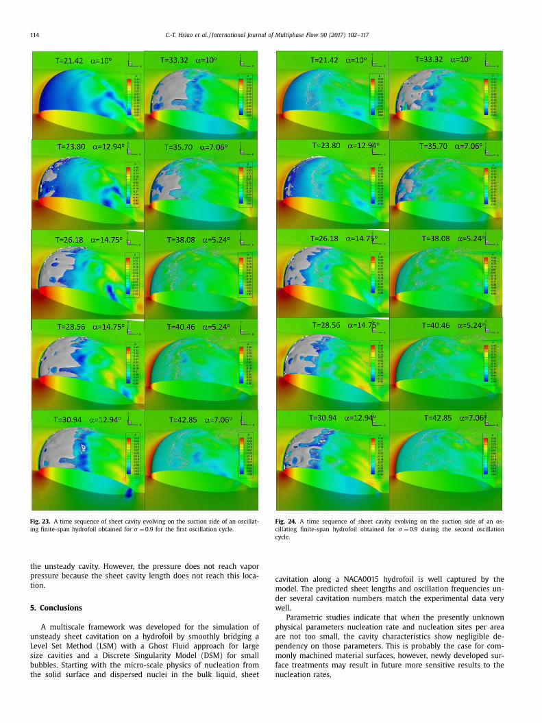
lation was continued up to the end of the third cycle. Figs. 24 and

5 show time sequences of the solutions for the second and third

ycles. The oscillatory behavior of the sheet cavity is observed to

ot change significantly between the second and the third cycle

ince numerical starting transition phase is completed during the

rst cycle.

A zoomed view of the root sheet cavity near the leading edge

uring the second cycle is shown in Fig. 26 . It is seen that the

heet cavity starts to form from the leading edge near the blade

ip. It then extends toward the root as the angle of attack in-

reases. However, unlike for the single phase flow solution, the

heet cavity does not reach its maximum extent before the hydro-

oil reaches the highest angle of attack. On the contrary, the sheet

avity continues to grow beyond the time the foil has the high-

st angle of attack. After reaching its maximum extent, the sheet

avity subsides without showing clear cloud shedding in this case.

his could be due to the corase grid resolution. Simulations with

much finer grid should be conducted in the future to clarify this

ehavior.

Fig. 27 shows a comparison of the time histories of the pressure

oefficient monitored at x = 0.04L (near leading edge) and x = 0.5L

middle chord) between the single-phase and the two-phase flow

omputations up to three cycles after the two-phase model was

urned on. The modifications of the pressure due to the sheet cav-

ty can be clearly seen at both locations. For the location near the

eading edge, the pressure at the hydrofoil surface becomes equal

o the vapor pressure ( C p = −0.9) once the sheet cavity reaches this

ocation. Pressure spikes are also observed as in the 2D computa-

ions due to the local breakup of the sheet cavity. For the location

t the mid-chord, the pressure is also changed by the presence of

114 C.-T. Hsiao et al. / International Journal of Multiphase Flow 90 (2017) 102–117

Fig. 23. A time sequence of sheet cavity evolving on the suction side of an oscillat-

ing finite-span hydrofoil obtained for σ = 0.9 for the first oscillation cycle.

Fig. 24. A time sequence of sheet cavity evolving on the suction side of an os-

cillating finite-span hydrofoil obtained for σ = 0.9 during the second oscillation

cycle.

c

m

d

w

p

a

p

m

f

n

the unsteady cavity. However, the pressure does not reach vapor

pressure because the sheet cavity length does not reach this loca-

tion.

5. Conclusions

A multiscale framework was developed for the simulation of

unsteady sheet cavitation on a hydrofoil by smoothly bridging a

Level Set Method (LSM) with a Ghost Fluid approach for large

size cavities and a Discrete Singularity Model (DSM) for small

bubbles. Starting with the micro-scale physics of nucleation from

the solid surface and dispersed nuclei in the bulk liquid, sheet

avitation along a NACA0015 hydrofoil is well captured by the

odel. The predicted sheet lengths and oscillation frequencies un-

er several cavitation numbers match the experimental data very

ell.

Parametric studies indicate that when the presently unknown

hysical parameters nucleation rate and nucleation sites per area

re not too small, the cavity characteristics show negligible de-

endency on those parameters. This is probably the case for com-

only machined material surfaces, however, newly developed sur-

ace treatments may result in future more sensitive results to the

ucleation rates.

C.-T. Hsiao et al. / International Journal of Multiphase Flow 90 (2017) 102–117 115

Fig. 25. A time sequence of sheet cavity evolving on the suction side of an oscillat-

ing finite-span hydrofoil obtained for σ = 0.9 for the third oscillation cycle.

t

l

f

s

p

T

w

Fig. 26. Zoomed view of the root sheet cavity near the leading edge obtained for

σ = 0.9.

c

fl

s

s

w

p

i

t

A

d

s

Sensitivity assessment of the threshold values of the switch cri-

eria between discreet microbubbles and large cavities also shows

ittle dependency on the parameters as long as the size criterion

or transforming a nuclei bubble into a large cavity is not too

mall.

The developed multiscale two-phase flow model was also ap-

lied to simulate sheet and cloud cavitation on 3D lifting surface.

hree-dimensional simulations for the 2D NACA0015 foil capture

ell sheet cavitation dynamics and cloud shedding with a more

omplicated breakup observed due to the 3D unsteadiness of the

ow.

Sheet cavitation on an oscillating finite-span hydrofoil was also

imulated using the developed model and a moving overset grid

cheme. Although the unsteady development of the sheet cavity

as also captured, the result do not show yet clear cloud shedding

robably due to inadequate grid resolution. This will be improved

n future effort s by refining the grids and conducting longer dura-

ion simulations.

cknowledgments

This work was supported by the Office of Naval Research un-

er contract N0 0 014-12-C-0382 monitored by Dr. Ki-Han Kim. This

upport is highly appreciated.

116 C.-T. Hsiao et al. / International Journal of Multiphase Flow 90 (2017) 102–117

Fig. 27. Comparison of time histories of the pressure coefficients monitored at: (a) x = 0.04 L (near the leading edge), and (b) x = 0.5 L (mid-chord) for single phase and

two-phase flow computations.

H

H

H

H

H

K

K

K

K

KK

M

M

M

M

M

O

R

R

S

References

Atchley, A .A . , Prosperetti, A. , 1989. The crevice model of bubble nucleation. J. Acoust.Soc. Am. 86 (3), 1065–1084 .

Balachandar, S. , Eaton, J.K. , 2010. Turbulent dispersed multiphase flow. Ann. Rev.Fluid Mech. 42, 111–133 .

Berntsen, G.S. , Kjeldsen, M. , Arndt, R.E. , 2001. Numerical modeling of sheet and tip

vortex cavitation with FLUENT 5. Fourth International Symposium on Cavitation.NTNU .

Biesheuvel, A. , van Wijngaarden, L. , 1984. Two-phase flow equations for a dilutedispersion of gas bubble in liquid. J. Fluid Mech. 148, 301–318 .

Billet, M.L. , June 1985. Cavitation nuclei measurements – a review. ASME Cavitationand Multiphase Flow Forum,” FED, 23 .

Briggs, L.J. , 2004. Limiting negative pressure of water. J. Appl. Phys. 21 (7), 721–722 .

Boulon, O. , 1996. Etude Expérimentale de la Cavitation de Tourbillon Marginal –Effets Instationnaires de Germes et de Confinement. Institut National Polytech-

nique de Grenoble . Chahine, G.L. , Duraiswami, R. , 1992. Dynamical interactions in a multi-bubble cloud.

J. Fluids Eng. 114 (4), 6 80–6 86 . Chahine, G.L. , Hsiao, C.-T. , 20 0 0. Modeling 3-D unsteady sheet cavities using a cou-

pled UnRANS-BEM code. In: Proceedings of the 23rd Symposium on Naval Hy-

drodynamics. Val De Reuil, France September 17-22 . Chahine, G.L. , 2004. Nuclei effects on cavitation inception and noise. Keynote pre-

sentation, 25th Symposium on Naval Hydrodynamics Aug. 8-13 . Chahine, G.L. , 2009. Numerical simulation of bubble flow interactions. J. Hydrodyn.

Ser. B 21 (3), 316–332 . Chen, Y. , Heister, D.D. , 1994. A numerical treatment for attached cavitation. J. Fluids

Eng. 116, 613–618 . Choi, J.-K. , Hsiao, C.-T. , Chahine, G.L. , 2004. Tip vortex cavitation inception study us-

ing the surface averaged pressure (SAP) model combined with a bubble splitting

model. 25th Symposium on Naval Hydrodynamics . Chorin, A.J. , 1967. A numerical method for solving incompressible viscous flow prob-

lems. J. Comput. Phys. 2, 12–26 . Dabiri, S. , Sirignano, W.A. , Joseph, D.D. , 2007. Cavitation in an orifice flow. Phys.

Fluids 19 . Dabiri, S. , Sirignano, W.A. , Joseph, D.D. , 2008. Two-dimensional and axisymmetric

viscous flow in apertures. J Fluid Mech 605, 1–18 .

Deshpande, M. , Feng, J. , Merkle, C.L. , 1993. Navier–Stokes analysis of 2D cavity flows.In: Cavitation Multiphase Flow FED, 153, pp. 149–155 .

Druzhinin, O.A. , Elghobashi, S. , 1998. Direct numerical simulations of bubble-ladenturbulent flows using the two-fluid formulation. Phys. Fluids 10, 685–697 .

Druzhinin, O.A. , Elghobashi, S. , 1999. A Lagrangian–Eulerian mapping solver fordirect numerical simulation of bubble-laden turbulent shear flows using the

two-fluid formulation. J. Comput. Phys. 154, 174–196 .

Druzhinin, O.A. , Elghobashi, S. , 2001. Direct numerical simulation of a three-dimen-sional spatially developing bubble-laden mixing layer with two-way coupling. J.

Fluid Mech. 429, 23–62 . Fedkiw, R.P. , Aslam, T. , Merriman, B. , Osher, S. , 1999. A non-oscillatory eulerian ap-

proach to interfaces in multimaterial flows (the ghost fluid method). J. Comput.Phys. 169, 463–502 .

Franklin, R.E. , 1992. A note on the radius distribution function for microbubbles

of gas in water. In: ASME Cavitation and Multiphase Flow Forum, FED, 135,pp. 77–85 .

Haberman, W.L. , Morton, R.K. , 1953. An Experimental Investigation of the Drag andShape of Air Bubble Rising in Various Liquids DTMB Report 802 .

Harvey, E.N. , et al. , 1944. Bubble formation in animals. II. gas nuclei and their dis-tribution in blood and tissues. J. Cell. Comp. Physiol. 24 (1), 23–34 .

irschi, R. , Dupont, P. , Avellan, F. , 1998. Partial sheet cavities prediction on a twistedelliptical platform hydrofoil using a fully 3-D approach. In: Proceedings 3rd in-

ternational Symposium on Cavitation, Vol. 1. Grenoble, France .

siao, C.-T. , Chahine, G. , 2004. Prediction of tip vortex cavitation inception usingcoupled spherical and nonspherical bubble models and Navier–Stokes computa-

tions. J. Mar. Sci. Technol. 8 (3), 99–108 . siao, C.-T. , Chahine, G. , 2008. Numerical study of cavitation inception due to vor-

tex/vortex interaction in a ducted propulsor. J. Ship Res. 52 (2), 114–123 . siao, C.-T. , Chahine, G.L. , Liu, H.-L. , 2003. Scaling effect on prediction of cavitation

inception in a line vortex flow. J. Fluids Eng. 125 (1), 53–60 .

siao, C.T. , Wu, X. , Ma, J. , Chahine, G.L. , 2013. Numerical and experimental study ofbubble entrainment due to a horizontal plunging jet. Int. Shipbuilding Prog. 60

(1), 435–469 . ang, M. , Fedkiw , Liu, L.D. , 20 0 0. A boundary condition capturing method for mul-

tiphase incompressible flow. J. Sci. Comp. 15, 323–360 . Kawamura, T. , Sakoda, M. , 2003. Comparison of bubble and sheet cavitation models

for simulation of cavitating flow over a hydrofoil. Fifth International Symposiumon Cavitation, November 1-4 .

innas, S.A. , Fine, N.E. , 1993. A numerical nonlinear analysis of the flow around two-

and three-dimensional partially cavitating hydrofoils. J. Fluid. Mech. 254 . inzel, M.P. , Lindau, J.W. , Kunz, R.F. , 2009. A level-set approach for large scale cavi-

tation. DoD High Performance Computing Modernization Program Users GroupConference June 15-18 .

odama, Y. , Take, N. , Tamiya, S. , Kato, H. , 1981. The effect of nuclei on the inceptionof bubble and sheet cavitation on axisymmetric bodies. J Fluids Eng 103 (4),

557–563 Dec 01 .

uiper, G. “Cavitation in Ship Propulsion,” TU Delft, Jan. 15, 2010. unz, R.F. , Boger, D.A. , Stinebring, D.R. , Chyczewski, T.S. , Lindau, J.W. , Gibeling, H.J. ,

20 0 0. A preconditioned navier-stokes method for two-phase flows with appli-cation to cavitation. Comput. Fluids 29, 849–875 .

a, J. , et al. , 2011. Two-fluid modeling of bubbly flows around surface ships using aphenomenological subgrid air entrainment model. Comput. Fluids 52, 50–57 .

a, J. , et al. , 2012. A two-way coupled polydispersed two-fluid model for the simu-

lation of air entrainment beneath a plunging liquid jet. ASME J. Fluids Eng. 134(10) .

a, J. , Hsiao, C.-T. , Chahine, G.L. , 2015a. Euler–Lagrange simulations of bubble clouddynamics near a wall. ASME J. Fluid Eng. 137 (4), 041301 .

Ma, J. , Hsiao, C.-T. , Chahine, G.L. , 2015b. Spherical bubble dynamics in a bubblymedium using an euler-lagrange model corresponding. Chem. Eng. 128, 64–81 .

edwin, H. , 1977. Counting bubbles acoustically: a review. Ultrasonics 15, 7–13 .

Merkle, C.L. , Feng, J. , Buelow, P.E.O. , 1998. Computational modeling of the dynam-ics of sheet cavitation. In: Proceedings of the 3rd International Symposium on

Cavitation, (CAV1998). Grenoble, France . ørch, K.A. , 2009. Cavitation nuclei: experiments and theory. J. Hydrodyn. Ser. B 21

(2), 176–189 . sher, S. , Fedkiw, R.P. , 2001. Level set methods, an overview and some recent re-

sults. J. Comput. Phys. 169, 463–502 .

aju, R. , Singh, S. , Hsiao, C.-S. , Chahine, G. , 2011. Study of pressure wave propagationin a two-phase bubbly mixture. Trans. ASME-I-J. Fluids Eng. 133 (12), 121302 .

oe, P.L. , 1981. Approximate riemann solvers, parameter vectors, and differenceschemes. J. Comput. Phys. 43, 357–372 .

affman, P.G. , 1965. The lift on a small sphere in a slow shear flow. J. Fluid Mech.22, 385–400 .

Singhal, N.H. , Athavale, A.K. , Li, M. , Jiang, Y. , 2002. Mathematical basis and validation

of the full cavitation model. J. Fluids Eng. 124, 1–8 . Shen, Y. , Dimotakis, P. , 1989. The influence of surface cavitation on hydrodynamic

forces. American Towing Tank Conference, 22nd .

C.-T. Hsiao et al. / International Journal of Multiphase Flow 90 (2017) 102–117 117

S

v

V

V

S

F

X

Y

Y

W

Z

Z

ussman, M. , Smereka, P. , Osher, S. , 1998. An improved level set approach for in-compressible two-phase flows. J. Comp., Phys. 148, 81–124 .

an Leer, B. , Woodward, P.R. , 1979. The MUSCL code for compressible flow: philos-ophy and results. In: Proc. of the TICOM Conf. Austin, TX .

anden, K.J. , Whitfield, D.L. , 1995. Direct and iterative algorithms for the three-di-mensional Euler equations. AIAA J. 33 (5), 851–858 .

arghese, A.N. , Uhlman, J.S. , Kirschner, I.N. , 2005. High speed bodies in partiallycavitating axisymmetric flow. J. Fluids Eng. 127, 41–54 .

hams, E. , Finn, J. , Apte, S. , 2011. A numerical scheme for Euler–Lagrange simula-

tion of bubbly flows in complex systems. Int. J. Numer. Methods Fluids 67 (12),1865–1898 .

errante, A. , Elghobashi, S. , 2004. On the physical mechanisms of drag reductionin a spatially developing turbulent boundary layer laden with microbubbles. J.

Fluid Mech. 503, 345–355 .

u, J. , Maxey, M.R. , Karniadakis, G.E. , 2002. Numerical simulation of turbulent dragreduction using micro-bubbles. J. Fluid Mech. 468, 271–281 .

ount, D.E. , 1979. Skins of varying permeability: a stabilization mechanism for gascavitation nuclei. J. Acoust. Soc. Am. 65 (6), 1429–1439 .

uan, W. , Sauer, J. , Schnerr, G.H. , 2001. Modeling and computation of unsteady cav-itation flows in injection nozzles. J. Mech. Ind. 2, 383–394 .

u, X. , Chahine, G.L. , 2010. Development of an acoustic instrument for bubble sizedistribution measurement. J. Hydrodyn. Ser. B 22 (5, Supplement 1), 330–336

Oct .

hang, D.Z. , Prosperetti, A. , 1994a. Averaged equations for inviscid dispersetwo-phase flow. J. Fluid Mech. 267, 185 .

hang, D.Z. , Prosperetti, A. , 1994b. Ensemble phase-averaged equations for bubblyflows. Phys. Fluids 6, 2956–2970 .