International Journal of Engineering (IJE) Volume (3) Issue (1)
Upload
cscjournalsCategory
view
4.091download
6

Editor in Chief Dr. Kouroush Jenab
International Journal of Engineering (IJE)
Book: 2009 Volume 3, Issue 2
Publishing Date: 31-04-2009
Proceedings
ISSN (Online): 1985-2312
This work is subjected to copyright. All rights are reserved whether the whole or
part of the material is concerned, specifically the rights of translation, reprinting,
re-use of illusions, recitation, broadcasting, reproduction on microfilms or in any
other way, and storage in data banks. Duplication of this publication of parts
thereof is permitted only under the provision of the copyright law 1965, in its
current version, and permission of use must always be obtained from CSC
Publishers. Violations are liable to prosecution under the copyright law.
IJE Journal is a part of CSC Publishers
http://www.cscjournals.org
©IJE Journal
Published in Malaysia
Typesetting: Camera-ready by author, data conversation by CSC Publishing
Services – CSC Journals, Malaysia
CSC Publishers

Table of Contents Volume 3, Issue 2, April 2009.
Pages
85 - 119
120 - 147
148 - 158
A Review onModeling of Hybrid Solid Oxide Fuel Cell Systems
Farshid Zabihian, Alan Fung.
An Overview of the Integration of Advanced Oxidation
Technologies And Other Processes For Water And Wastewater
Treatment
Masroor Mohajerani, Mehrab Mehrvar, Farhad Ein-Mozaffari.
Development of on Chip Devices for Life Science Applications
Stephanus Büttgenbach, Anne Balck, Stefanie Demming,
Claudia Lesche, Monika Michalzik, Alaaldeen.
159 - 173
174 - 184
Fuel and GHG Emission Reduction Potentials by Fuel Switching
and Technology Improvement in the Iranian Electricity Generation
Sector
Farshid Zabihian, Alan Fung.
Water Sloshing in Rectangular Tanks – An Experimental
Investigation & Numerical Simulation
Lyes Khezzar, Abdennour C Seibi, Afshin Goharzadeh.

185 - 200
Multi-dimentional upwind schemes for the Euler Equations on
unstructured grids
Mounir Aksas, Abdelmouman H. Benmachiche.
201 – 219
Availability Analysis of A Cattle Feed Plant Using Matrix Method
Deepika Garg, Kuldeep Kumar, Jai Singh.
International Journal of Engineering, (IJE) Volume (3) : Issue (2)

S. Büttgenbach, A. Balck, S. Demming, C. Lesche, M. Michalzik, A. T. Al-Halhouli
International Journal of Engineering 1
Development of on Chip Devices for Life Science Applications
S. Büttgenbach [email protected] Institute for Microtechnology Technische Universität Braunschweig Alte Salzdahlumer Str.203, 38126 Braunschweig, Germany A. Balck [email protected] Institute for Microtechnology Technische Universität Braunschweig Alte Salzdahlumer Str.203, 38126 Braunschweig, Germany S. Demming [email protected] Institute for Microtechnology Technische Universität Braunschweig Alte Salzdahlumer Str.203, 38126 Braunschweig, Germany C. Lesche [email protected] Institute for Microtechnology Technische Universität Braunschweig Alte Salzdahlumer Str.203, 38126 Braunschweig, Germany M. Michalzik Institute for Microtechnology Technische Universität Braunschweig Alte Salzdahlumer Str.203, 38126 Braunschweig, Germany A. T. Al-Halhouli [email protected] Institute for Microtechnology Technische Universität Braunschweig Alte Salzdahlumer Str.203, 38126 Braunschweig, Germany
Abstract
This work reports on diverse technologies implemented for fabricating microfluidic devices such as biomedical micro sensors, micro pumps, bioreactors and micro separators. UV depth lithography and soft lithography were applied in the fabrication processes using different materials, for example SU-8, polydimethylsiloxane (PDMS), silicon, glass and ceramics. Descriptions of the fabrication process of completed devices and their performance are provided. Experimental tests and results are presented where available. This work highlights the importance of down scaling in producing efficient devices suitable for life science applications using diverse materials that are compatible with chemical and biomedical applications. Keywords: Microfluidics, Biosensors, Bioreactors, UV depth lithography, soft lithography.

S. Büttgenbach, A. Balck, S. Demming, C. Lesche, M. Michalzik, A. T. Al-Halhouli
International Journal of Engineering 2
1. INTRODUCTION Microfluidics is an exciting field of science and engineering that enables very small-scale fluid control and analysis, and allows instrument manufacturers to develop smaller, cost-effective and powerful systems. It also offers potential benefits in chemistry, biology, and medicine through minimized sample volume, fast detection, usability for non specialized staff, temperature stability, reduced reagents consumption, decreased analysis time, etc [1]. This work presents the optimized process technologies used by the Institute for Microtechnology (IMT) research group for fabricating microfluidic devices (e.g. dispersion microelements, micro pumps, bioreactors, blood separator and Quartz crystal microbalance (QCM)). These devices are suitable for life science applications and can be integrated on chip.
2. SILICON BASED MICROFLUIDIC DEVICES Nanoparticles gain more and more in importance. A major process during handling of nanoparticles especially for the formulation of pharmaceutical, cosmetic and biotechnological products is the dispersion. While mixing the nanoparticles into a fluid, the nanoparticles agglomerate to each other. Dispersion describes the agglomerate breakup as well as the homogeneous distribution of particles in the surrounding fluid. The dispersion process within a micro-system offers the following two main advantages: generation of the high energy density required for dispersion of nano-sized particles, and use of extremely low volumes of reactants. Hence, micro-systems afford an excellent approach for pharmaceutical and biotechnological screening applications. To generate the high stress intensities, which are necessary to disperse agglomerates into primary particles, a new dispersion micro-element has been developed at IMT. The designed micro-elements (Fig.1) consist of a 20 mm long channel with 1 mm diameter inlet and outlet ports at both ends.
FIGURE 1: Function principle of the dispersion micro-element The central part of the micro-channels features different geometries varying from elementary angular and circular alternatives to more complex geometries with multiple streams (Fig. 2). Furthermore, diverse barrier structures are also included. In the different designs, the width of the micro channel varies from 76 µm to 1 mm. In addition to using the dispersion effect of the micro-elements, it is planned to compress the nanoparticle suspension with high pressure, comparable to macroscopic apparatus, through the micro-channels. Therefore a resilient material was needed, that is simultaneously able to be fabricated into a micro-channel with precise and rectangular walls. For these reasons silicon was chosen in combination with dry etching for the fabrication process.

S. Büttgenbach, A. Balck, S. Demming, C. Lesche, M. Michalzik, A. T. Al-Halhouli
International Journal of Engineering 3
FIGURE 2: Different micro-channel designs To realize both a leak-proof micro-channel and an unrestricted visibility of the dispersion process in the micro-element, glass was chosen as a coating material. The structuring of glass is a difficult and extensive process, which often entails producing material stresses in the treatment affected zone. In this case, where the inlet and outlet are under high pressure, micro-cracks are especially disadvantageous. To avoid this problem and to achieve a maximum stability in the dispersion micro-element, we used a technique of double-sided etching of silicon.
FIGURE 3: Batch fabrication process of the dispersion micro-element Standard UV photolithography is used to structure the aluminum layers, which are sputtered on both sides of a silicon wafer (Fig. 3a). After wet chemical etching in Al-etching solution, the photoresist layer is removed, whereby the aluminum structures remain (Fig. 3b). The desired micro-structures are now etched into the silicon base material. A deep reactive ion etching (DRIE) process, also known as Bosch process, has been used for this purpose. More details concerning the fabrication process are presented in [2]. The alternating process sequence from etching (with SF6) and passivation (with C4F8) allows extremely high aspect ratios and almost rectangular walls. First the channel geometry is etched from the top side to a depth of 200 µm into the silicon wafer (Fig. 3c). In a following etch step the wafer is flipped and the inlet and outlet are etched from the bottom side until they meet the channel bottom (Fig. 3d). After the aluminum masking layer is removed in a wet chemical etching step, the upper side is coated with a glass wafer in an
S. Büttgenbach, A. Balck, S. Demming, C. Lesche, M. Michalzik, A. T. Al-Halhouli
International Journal of Engineering 4
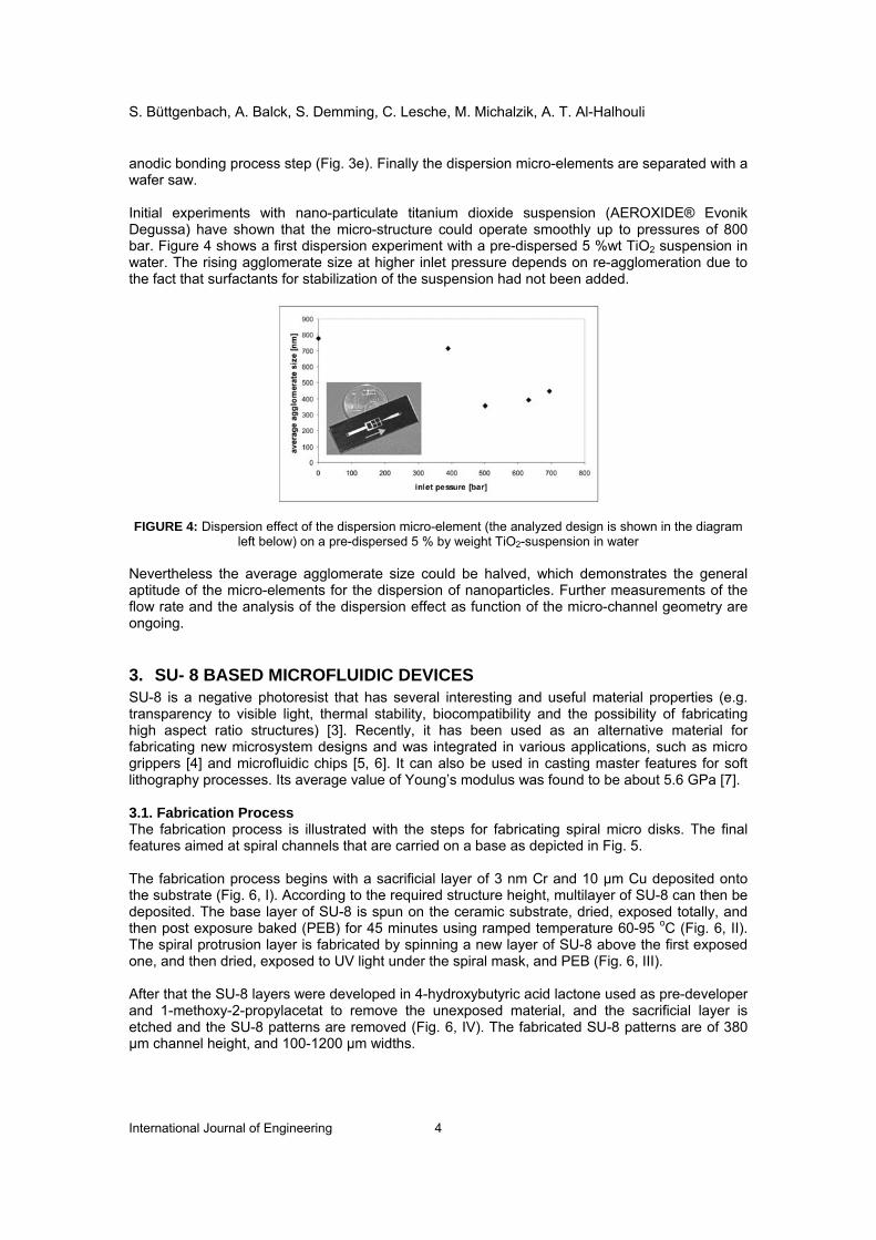
anodic bonding process step (Fig. 3e). Finally the dispersion micro-elements are separated with a wafer saw. Initial experiments with nano-particulate titanium dioxide suspension (AEROXIDE® Evonik Degussa) have shown that the micro-structure could operate smoothly up to pressures of 800 bar. Figure 4 shows a first dispersion experiment with a pre-dispersed 5 %wt TiO2 suspension in water. The rising agglomerate size at higher inlet pressure depends on re-agglomeration due to the fact that surfactants for stabilization of the suspension had not been added.
FIGURE 4: Dispersion effect of the dispersion micro-element (the analyzed design is shown in the diagram left below) on a pre-dispersed 5 % by weight TiO2-suspension in water
Nevertheless the average agglomerate size could be halved, which demonstrates the general aptitude of the micro-elements for the dispersion of nanoparticles. Further measurements of the flow rate and the analysis of the dispersion effect as function of the micro-channel geometry are ongoing.
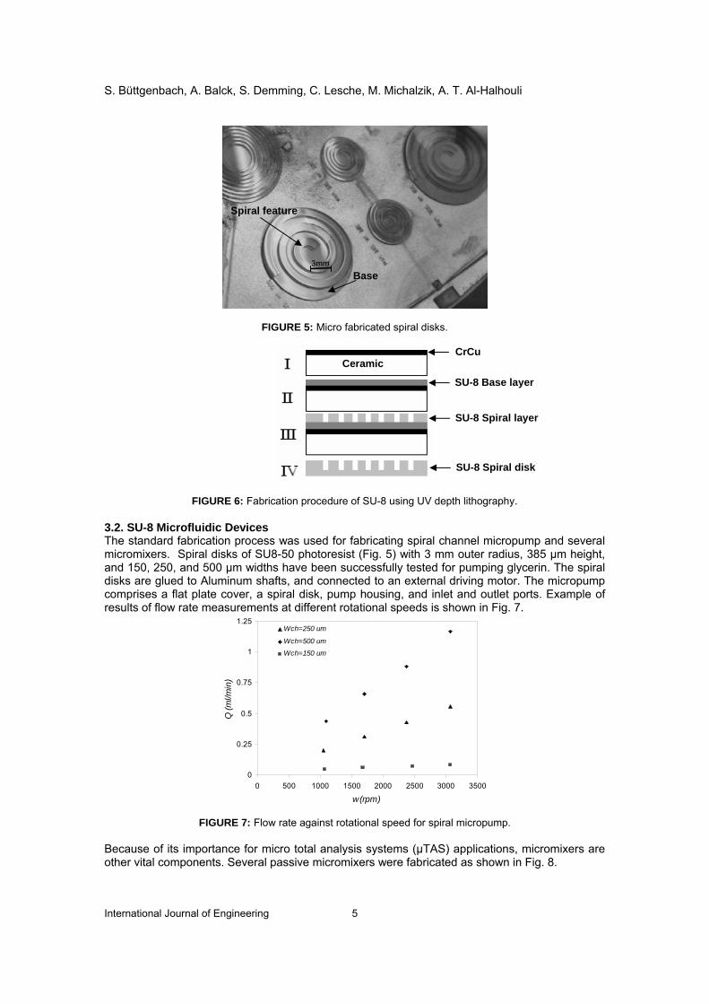
3. SU- 8 BASED MICROFLUIDIC DEVICES SU-8 is a negative photoresist that has several interesting and useful material properties (e.g. transparency to visible light, thermal stability, biocompatibility and the possibility of fabricating high aspect ratio structures) [3]. Recently, it has been used as an alternative material for fabricating new microsystem designs and was integrated in various applications, such as micro grippers [4] and microfluidic chips [5, 6]. It can also be used in casting master features for soft lithography processes. Its average value of Young’s modulus was found to be about 5.6 GPa [7]. 3.1. Fabrication Process The fabrication process is illustrated with the steps for fabricating spiral micro disks. The final features aimed at spiral channels that are carried on a base as depicted in Fig. 5. The fabrication process begins with a sacrificial layer of 3 nm Cr and 10 µm Cu deposited onto the substrate (Fig. 6, I). According to the required structure height, multilayer of SU-8 can then be deposited. The base layer of SU-8 is spun on the ceramic substrate, dried, exposed totally, and then post exposure baked (PEB) for 45 minutes using ramped temperature 60-95 oC (Fig. 6, II). The spiral protrusion layer is fabricated by spinning a new layer of SU-8 above the first exposed one, and then dried, exposed to UV light under the spiral mask, and PEB (Fig. 6, III). After that the SU-8 layers were developed in 4-hydroxybutyric acid lactone used as pre-developer and 1-methoxy-2-propylacetat to remove the unexposed material, and the sacrificial layer is etched and the SU-8 patterns are removed (Fig. 6, IV). The fabricated SU-8 patterns are of 380 µm channel height, and 100-1200 µm widths.
S. Büttgenbach, A. Balck, S. Demming, C. Lesche, M. Michalzik, A. T. Al-Halhouli
International Journal of Engineering 5
FIGURE 5: Micro fabricated spiral disks.
FIGURE 6: Fabrication procedure of SU-8 using UV depth lithography. 3.2. SU-8 Microfluidic Devices The standard fabrication process was used for fabricating spiral channel micropump and several micromixers. Spiral disks of SU8-50 photoresist (Fig. 5) with 3 mm outer radius, 385 µm height, and 150, 250, and 500 µm widths have been successfully tested for pumping glycerin. The spiral disks are glued to Aluminum shafts, and connected to an external driving motor. The micropump comprises a flat plate cover, a spiral disk, pump housing, and inlet and outlet ports. Example of results of flow rate measurements at different rotational speeds is shown in Fig. 7.
0
0.25
0.5
0.75
1
1.25
0 500 1000 1500 2000 2500 3000 3500
w (rpm)
Q (m
l/min
)
Wch=250 um
Wch=500 um
Wch=150 um
FIGURE 7: Flow rate against rotational speed for spiral micropump. Because of its importance for micro total analysis systems (µTAS) applications, micromixers are other vital components. Several passive micromixers were fabricated as shown in Fig. 8.
Base
Spiral feature
Ceramic CrCu
SU-8 Base layer
SU-8 Spiral layer
SU-8 Spiral disk
3mm
S. Büttgenbach, A. Balck, S. Demming, C. Lesche, M. Michalzik, A. T. Al-Halhouli
International Journal of Engineering 6
FIGURE 8: Micromixer [8].
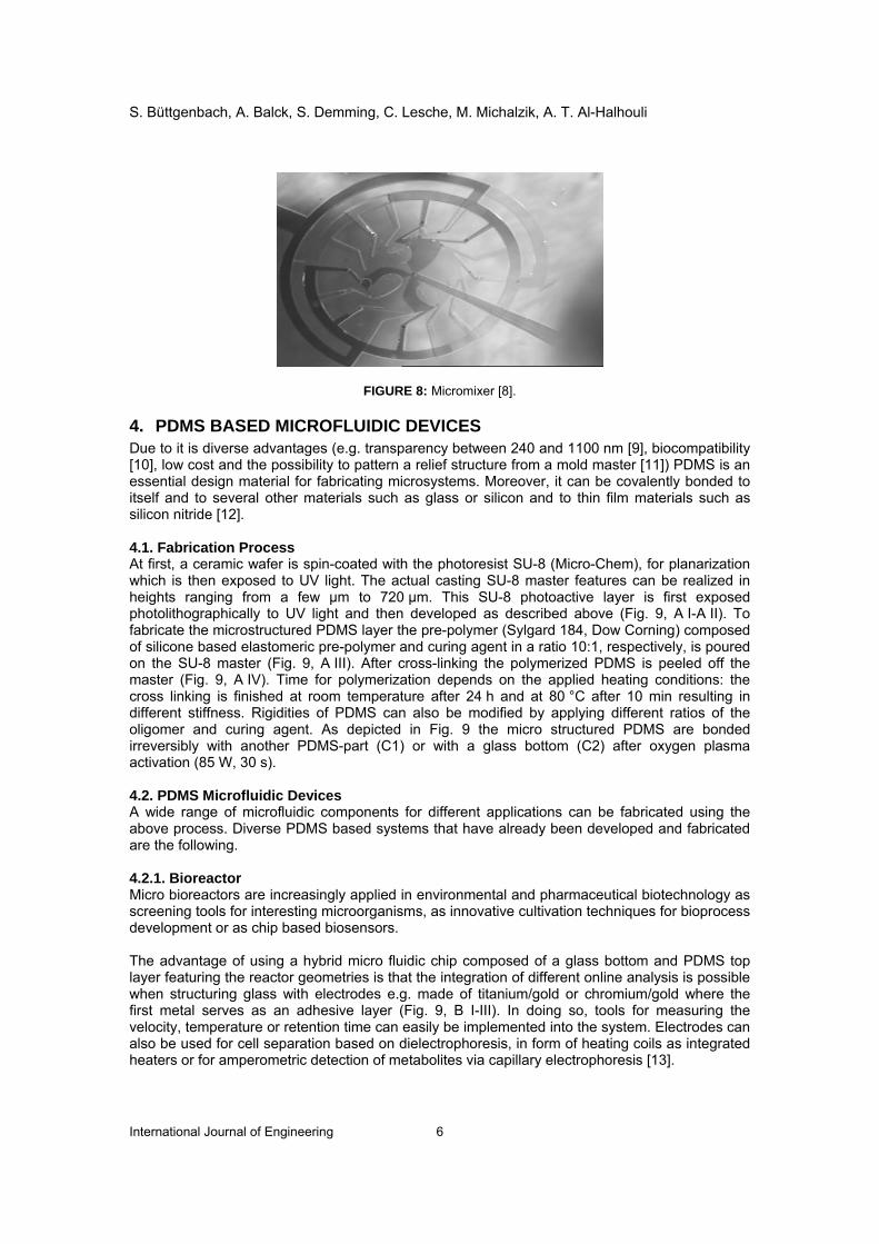
4. PDMS BASED MICROFLUIDIC DEVICES Due to it is diverse advantages (e.g. transparency between 240 and 1100 nm [9], biocompatibility [10], low cost and the possibility to pattern a relief structure from a mold master [11]) PDMS is an essential design material for fabricating microsystems. Moreover, it can be covalently bonded to itself and to several other materials such as glass or silicon and to thin film materials such as silicon nitride [12]. 4.1. Fabrication Process At first, a ceramic wafer is spin-coated with the photoresist SU-8 (Micro-Chem), for planarization which is then exposed to UV light. The actual casting SU-8 master features can be realized in heights ranging from a few µm to 720 μm. This SU-8 photoactive layer is first exposed photolithographically to UV light and then developed as described above (Fig. 9, A I-A II). To fabricate the microstructured PDMS layer the pre-polymer (Sylgard 184, Dow Corning) composed of silicone based elastomeric pre-polymer and curing agent in a ratio 10:1, respectively, is poured on the SU-8 master (Fig. 9, A III). After cross-linking the polymerized PDMS is peeled off the master (Fig. 9, A IV). Time for polymerization depends on the applied heating conditions: the cross linking is finished at room temperature after 24 h and at 80 °C after 10 min resulting in different stiffness. Rigidities of PDMS can also be modified by applying different ratios of the oligomer and curing agent. As depicted in Fig. 9 the micro structured PDMS are bonded irreversibly with another PDMS-part (C1) or with a glass bottom (C2) after oxygen plasma activation (85 W, 30 s). 4.2. PDMS Microfluidic Devices A wide range of microfluidic components for different applications can be fabricated using the above process. Diverse PDMS based systems that have already been developed and fabricated are the following. 4.2.1. Bioreactor Micro bioreactors are increasingly applied in environmental and pharmaceutical biotechnology as screening tools for interesting microorganisms, as innovative cultivation techniques for bioprocess development or as chip based biosensors. The advantage of using a hybrid micro fluidic chip composed of a glass bottom and PDMS top layer featuring the reactor geometries is that the integration of different online analysis is possible when structuring glass with electrodes e.g. made of titanium/gold or chromium/gold where the first metal serves as an adhesive layer (Fig. 9, B I-III). In doing so, tools for measuring the velocity, temperature or retention time can easily be implemented into the system. Electrodes can also be used for cell separation based on dielectrophoresis, in form of heating coils as integrated heaters or for amperometric detection of metabolites via capillary electrophoresis [13].
S. Büttgenbach, A. Balck, S. Demming, C. Lesche, M. Michalzik, A. T. Al-Halhouli
International Journal of Engineering 7
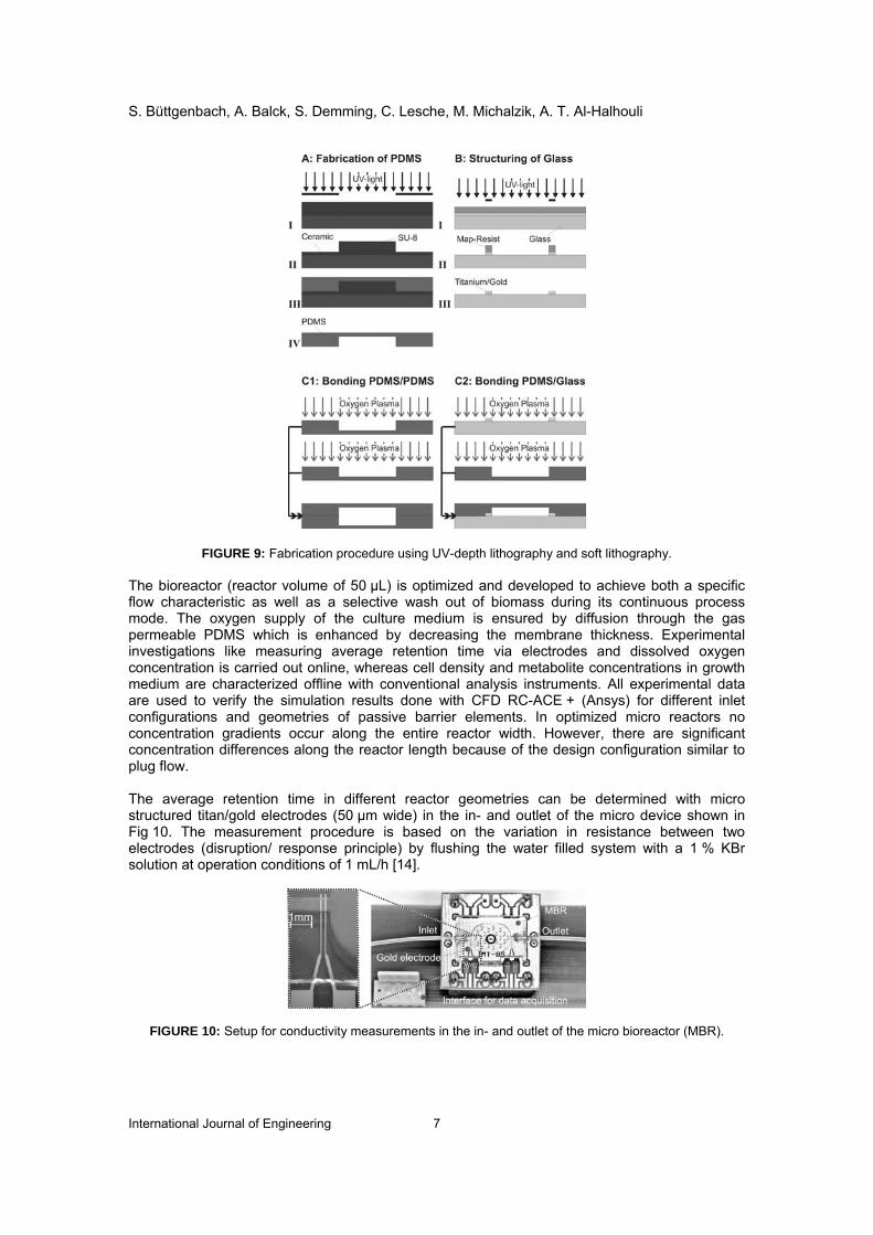
FIGURE 9: Fabrication procedure using UV-depth lithography and soft lithography. The bioreactor (reactor volume of 50 µL) is optimized and developed to achieve both a specific flow characteristic as well as a selective wash out of biomass during its continuous process mode. The oxygen supply of the culture medium is ensured by diffusion through the gas permeable PDMS which is enhanced by decreasing the membrane thickness. Experimental investigations like measuring average retention time via electrodes and dissolved oxygen concentration is carried out online, whereas cell density and metabolite concentrations in growth medium are characterized offline with conventional analysis instruments. All experimental data are used to verify the simulation results done with CFD RC-ACE + (Ansys) for different inlet configurations and geometries of passive barrier elements. In optimized micro reactors no concentration gradients occur along the entire reactor width. However, there are significant concentration differences along the reactor length because of the design configuration similar to plug flow. The average retention time in different reactor geometries can be determined with micro structured titan/gold electrodes (50 µm wide) in the in- and outlet of the micro device shown in Fig 10. The measurement procedure is based on the variation in resistance between two electrodes (disruption/ response principle) by flushing the water filled system with a 1 % KBr solution at operation conditions of 1 mL/h [14].
FIGURE 10: Setup for conductivity measurements in the in- and outlet of the micro bioreactor (MBR).
S. Büttgenbach, A. Balck, S. Demming, C. Lesche, M. Michalzik, A. T. Al-Halhouli
International Journal of Engineering 8
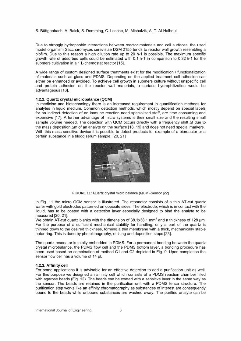
Due to strongly hydrophobic interactions between reactor materials and cell surfaces, the used model organism Saccharomyces cerevisiae DSM 2155 tends to reactor wall growth resembling a biofilm. Due to this reason a high dilution rate up to 20 h-1 is possible. The maximum specific growth rate of adsorbed cells could be estimated with 0.1 h-1 in comparison to 0.32 h-1 for the submers cultivation in a 1 L-chemostat reactor [15]. A wide range of custom designed surface treatments exist for the modification / functionalization of materials such as glass and PDMS. Depending on the applied treatment cell adhesion can either be enhanced or avoided. To achieve cell growth in submers culture without unspecific cell and protein adhesion on the reactor wall materials, a surface hydrophilization would be advantageous [16]. 4.2.2. Quartz crystal microbalance (QCM) In medicine and biotechnology there is an increased requirement in quantification methods for analytes in liquid medium. Common detection methods, which mostly depend on special labels for an indirect detection of an immune reaction need specialized staff, are time consuming and expensive [17]. A further advantage of micro systems is their small size and the resulting small sample volume needed. The detection with QCM occurs directly with a frequency shift Δf due to the mass deposition Δm of an analyte on the surface [18, 19] and does not need special markers. With this mass sensitive device it is possible to detect products for example of a bioreactor or a certain substance in a blood serum sample. [20, 21]
FIGURE 11: Quartz crystal micro balance (QCM)-Sensor [22] In Fig. 11 the micro QCM sensor is illustrated. The resonator consists of a thin AT-cut quartz wafer with gold electrodes patterned on opposite sides. The electrode, which is in contact with the liquid, has to be coated with a detection layer especially designed to bind the analyte to be measured [20, 21]. We obtain AT-cut quartz blanks with the dimension of 38.1x38.1 mm2 and a thickness of 128 µm. For the purpose of a sufficient mechanical stability for handling, only a part of the quartz is thinned down to the desired thickness, forming a thin membrane with a thick, mechanically stable outer ring. This is done by photolithography, etching and deposition steps [23]. The quartz resonator is totally embedded in PDMS. For a permanent bonding between the quartz crystal microbalance, the PDMS flow cell and the PDMS bottom layer, a bonding procedure has been used based on combination of method C1 and C2 depicted in Fig. 9. Upon completion the sensor flow cell has a volume of 14 µL. 4.2.3. Affinity cell For some applications it is advisable for an effective detection to add a purification unit as well. For this purpose we designed an affinity cell which consists of a PDMS reaction chamber filled with agarose beads (Fig. 12). The beads can be coated with a sensitive layer in the same way as the sensor. The beads are retained in the purification unit with a PDMS fence structure. The purification step works like an affinity chromatography as substances of interest are consequently bound to the beads while unbound substances are washed away. The purified analyte can be

S. Büttgenbach, A. Balck, S. Demming, C. Lesche, M. Michalzik, A. T. Al-Halhouli
International Journal of Engineering 9
subsequently detected with the quartz resonator with less interfering interactions from impurities [17].
FIGURE 12: Affinity cell [17] 4.2.4. Blood separation system It is important for the detection of serum proteins and to prevent the microstructure from blocking, that the blood serum is free of blood cells. To guarantee this, special structures have been developed and realized in PDMS as described in [24]. 4.2.5. Hydro-Gel Actuated Microvalve To handle different fluids needed for pre-purification and detection, special valves have to be used. In general blood proteins and biomolecules are very temperature sensitive so that the used valves may not warm during operation process. To guarantee this, valves with a pH sensitive hydrogel actuator were fabricated. The valve is composed of 5 PDMS layers as can be seen in Fig. 13. Layer 1 and 3 feature fluidic channels with height and width of 200 μm which are connected by a 200 µm hole in layer 2. This hole can be blocked by the expanding hydrogel pressing the 40 μm thick membrane (layer 4) down. The circular chamber for the hydrogel actuator has a diameter of 1500 μm. The hydrogel consists of the monomer 2-hydroxyethyl methacrylate (Sigma-Aldrich) and the copolymer acrylic acid (Sigma-Aldrich) in a 4:1 molar ratio. Ethylene glycol dimethacrylate (1 wt%, Sigma-Aldrich) was added as a crosslinker and Irgacure 651 (3 wt%, Sigma-Aldrich) as photoinitiator. Irgacure 651 is the registered name of 2,2-dimethoxy-2-phenyl acetophenone (Ciba Speciality Chemicals). A 5 mW UV-source with a wavelength of 366 nm was used for the exposure of the hydrogel through a mask in the microfluidic system.
FIGURE 13: Schematic and Picture of PDMS valve [24, 25]

S. Büttgenbach, A. Balck, S. Demming, C. Lesche, M. Michalzik, A. T. Al-Halhouli
International Journal of Engineering 10
To open and close the micro valve, pH 1 and pH 13 standard solutions have to be pumped through the hydrogel chamber, respectively. In Figure 13 a dye was injected into the fluid network to demonstrate function of the valve. [25, 26]
5. CONSLUSION The possibility of implementing available fabrication technologies at IMT for fabricating microfluidic devices using different materials has been described. Optimized processes showed high capability in handling several microfluidic applications under diverse conditions. This work highlights the advantages of micro technologies in biomedical applications.
ACKNOWLEDGEMENT This work has been supported in part by the Deutsche Forschungsgemeinschaft (DFG).
6. REFERENCES
1. V. Srinivasan, V. Pamula, R. Fair. “An Integrated digital microfluidic lab-on-a-chip for clinical diagnostics on human physiological fluids”. Lab on a Chip, 4:310-315, 2004.
2. F. Laermer, A. Urban. “Challenges, developments and applications of silicon deep reactive ion etching”. Microelectron. Eng. 67-68, 349-355, 2003.
3. H. Khoo, K. Liu, F. Tseng. “Mechanical strength and interfacial failure analysis of cantilevered SU-8 microposts”, J. Micromech. Microeng. 13:82-831, 2003.
4. B. Hoxhold, M. Kirchhoff, S. Bütefisch, S. Büttgenbach. “SMA Driven Micro Grippers Combining Piezo-Resistive Gripping Force Sensors with Epon SU-8 Mechanics”. XX Eurosensors 2006, Göteborg, 2006.
5. H. Sato, H. Matsumura, S. Keino, S. Shoji. “An all SU-8 microfluidic chip with built-in 3D fine microstructures”. J. Micromech. Microeng. 16:2318-2322, 2006.
6. J. Ribeiro, G. Minas, P. Turmezei, R. Wolffenbuttel, J. Correia. “A SU-8 fluidic microsystem for biological fluids analysis”. Sensors and Actuators A, 123-124:77-81, 2005.
7. A. Al-Halhouli, I. Kampen, T. Krah, S. Büttgenbach. “Nanoindentation testing of SU-8 photoresist mechanical properties”. Microelectronic Engineering, 85:942-944, 2008.
8. M. Feldmann, A. Waldschik, S. Büttgenbach. “A novel fabrication process for 3D-multilayer micro mixers”. Proc. 8th Int. Conf. on Miniaturized Systems for Chemistry and Life Sciences. Malmö, 2004.
9. S. Charati, S. Stern. “Diffusion of gases in silicone polymers: molecular dynamics simulations”. Macromolecules, 31:5529-5535, 1998.
10. W-J. Chang, D. Akin, M. Sedlak, M. R. Ladisch, R. Bashir. “Poly(dimethylsiloxane) (PDMS) and silicon hybrid biochip for bacterial culture”. Biomedical Microdevices, 5:281-290, 2003.
11. S. H. de Kock, J. C. du Preez, S. G. Kilian. “Anomalies in the growth kinetics of Saccharomyces cerevisiae strains in aerobic chemostat cultures”. Journal of Industrial Microbiology and Biotechnology, 24:231-236, 2000.
12. M. Feldmann, S. Demming, C. Lesche, S. Büttgenbach. “Novel Electromagnetic micropump”. Proceedings of SPIE, 2007.
13. R. Wilke, S. Büttgenbach. “A micromachined capillary electrophoresis chip with fully integrated electrodes for separation and electrochemical detection”. Biosensors and Bioelectronics, 19:149-153, 2003.

S. Büttgenbach, A. Balck, S. Demming, C. Lesche, M. Michalzik, A. T. Al-Halhouli
International Journal of Engineering 11
14. S. Demming, A. Jansen, E. Franco-Lara, R. Krull, S. Büttgenbach. “Mikroreaktorsystem als Screening-instrument für biologische Prozesse“. Proceedings of MicroSystemTechnology Congress, Dresden, 2007.
15. A. Edlich, S. Demming, M. Vogl, S. Büttgenbach, E. Franco-Lara, R. Krull. “Microfluidic Screening Reactor for Estimation of Biological Reaction Kinetics”. Proceedings of 1st European Congress on Microfluidics, Bologna, 2008.
16. J. M. Gancedo. “Control of pseudohyphae formation in Saccharomyces cerevisiae”. FEMS Microbiology Reviews, 25:107-123, 2001.
17. M. Michalzik, A. Balck, S. Büttgenbach, L. Al-Halabi, M. Hust, S: Dübel. “Microsensor System for Biochemical and Medical Analysis”, Proc. XX Eurosensors, Göteborg, 2006.
18. G. Sauerbrey. “Verwendung von Schwingquarzen zur Wägung dünner Schichten und zur Mikrowägung“. Zeitschrift für Physik A, 155:1546-1551, 1959.
19. C. K. O'Sullivan, G. Guilbault. “Commercial quartz crystal microbalances - theory and applications”. Biosensors and Bioelectronics, 14:663-670, 1999.
20. A. Balck, M. Michalzik, M. Wolff, U. Reichl, S. Büttgenbach. “Influenza virus detection in vaccine production with a quartz crystal microbalance”. Proceedings of Biosensors 2008, Shanghai, 2008.
21. M. Michalzik, L. Al-Halabi, A. Balck, M. Hust, S: Dübel, S. Büttgenbach. “A mass sensitivemicrofluidic immunosensor for CRP-detection using functional monolayers”. Proceedings of Biosensors 2008, Shanghai, 2008a.
22. M. Michalzik, A. Balck, L. Al-Halabi, M. Hust, S: Dübel, S. Büttgenbach. “Massensensitives Sensor-Fließsystem zur CRP-Diagnostik”. Proceedings of. Mikrosystemtechnikkongress, Dresden, 2007.
23. J. Rabe, S. Büttgenbach, B. Zimmermann, P. Hauptmann. Proceedings of IEEE/EIA International Frequency Control Symposium 2000.
24. A. Balck, A. T. Al-Halhouli, S. Büttgenbach. “Separation of blood cells in Y- microchannels”. ICTEA09, Abu Dhabi, 2009.
25. M. Michalzik, A. Balck, C. Ayala, N. Lucas, S. Demming, A. Phataralaoha, S. Büttgenbach. “A Hydrogel-Actuated Microvalve for Medical and Biochemical Sensing”. Actuator 08, Bremen, 2008b.
26. V. C. Ayala, M. Michalzik, S. Harling, H. Menzel, F. A. Guarnieri, S. Büttgenbach. “Design, Construction and Testing of a Monolithic pH-Sensitive Hydrogel-Valve for Biochemical and Medical Application”. Journal of Physics, Conference Series 90, 2007.

Farshid Zabihian, Alan Fung
International Journal of Engineering (IJE), Volume (3) : Issue (2) 85
A Review on Modeling of Hybrid Solid Oxide Fuel Cell Systems
Farshid Zabihian [email protected] Department of Mechanical and Industrial Engineering Ryerson University Toronto, M5B 2K3, Canada
Alan Fung [email protected] Department of Mechanical and Industrial Engineering Ryerson University Toronto, M5B 2K3, Canada
ABSTRACT
Over the past 2 decades, there has been tremendous progress on numerical and computational tools for fuel cells and energy systems based on them. The purpose of this work is to summarize the current status of hybrid solid oxide fuel cell (SOFC) cycles and identify areas that require further studies. In this review paper, a comprehensive literature survey on different types of SOFC hybrid systems modeling is presented. The paper has three parts. First, it describes the importance of the fuel cells modeling especially in SOFC hybrid cycles. Key features of the fuel cell models are highlighted and model selection criteria are explained. In the second part, the models in the open literature are categorized and discussed. It includes discussion on a detail example of SOFC-gas turbine cycle model, description of early models, models with different objectives such as parametric analysis, comparison of configurations, exergy analysis, optimization, non-stationary power generation applications, transient and off-design analysis, thermoeconomic analysis and so on. Finally, in the last section, key features of selected models are summarized and suggestions for areas that require further studies are presented. In this paper, a hybrid cycle can be any combination of SOFC and gas turbine, steam turbine, coal integrated gasification, and application in combined heat and power cycle. Keywords: Solid Oxide Fuel Cells, SOFC, Hybrid Energy Systems, Steady State and Dynamic Modeling.
1. INTRODUCTION
We owe our sophisticated society and current standard of living to energy infrastructure development and its consequences in the last century. But, global climate change and natural resources pollution cause significant worldwide concerns about current trend in energy systems development. According to the World Energy Outlook published by the International Energy Agency (IEA) [1], the world’s total electricity consumption would be doubled between 2003 and 2030. This report predicted that the share of fossil fuels as energy supplies for electricity generation will remain constant at nearly 65%. Power generation is responsible for half of the increase in global greenhouse gas emissions over the projection period. As a result of all these problems, sustainability considerations should be involved in all major energy development plans

Farshid Zabihian, Alan Fung
International Journal of Engineering (IJE), Volume (3) : Issue (2) 86
all over the world. There are various definitions for sustainability. Probably the simplest one is that sustainable activities are the activities that help existing generation to meet their needs without destroying the ability of future generations to meet theirs [2]. Fuel cells are very interesting alternative for conventional power generation technologies because of their high efficiency and very low environmental effects. In conventional power generation systems, fuel should be combusted to generate heat and then heat should be converted to mechanical energy, before it can be used to produce electrical energy. The maximum efficiency that a thermal engine can achieve is when it operates at Carnot cycle. The efficiency of this cycle is related to the ratio of the heat source and sink absolute temperature. However, fuel cells operation is based on electrochemical reactions and not fuel combustion; therefore, their efficiency is not limited by the thermodynamics laws and Carnot cycle. Instead, their efficiency is limited by the ratio of released Gibbs free energy to the inlet fuel heating value. It is interesting to note that this maximum efficiency is equal to the Carnot efficiency calculated at the temperature at which the combustion is reversible [3]. Furthermore, since there is no combustion, none of the pollutants, commonly produced by fuel combustors, is emitted. In this review paper, a comprehensive literature survey on different types of SOFC hybrid systems modeling is presented. It begins with a general discussion on roles of fuel cell and SOFC hybrid systems modeling and importance of review papers in this field. Then, key features of the fuel cell models are highlighted and model selection criteria are explained. In the second part, the models in the open literature are categorized and discussed based on selected criteria. Finally, in the last section, key features of selected models are summarized and suggestions for areas that require further studies are presented.
2. FUEL CELL MODELING
Simulation and mathematical models are certainly helpful for development of various power generation technologies; however, they are probably more important for fuel cell development. This is due to complexity of fuel cells and systems based on them, and the difficulty in experimentally characterizing their internal operation. This complexity can be explained based on the fact that within the fuel cell, tightly coupled electrochemical reactions, electrical conduction, ionic conduction, and heat transfer take place simultaneously. That is why a comprehensive study of fuel cells needs a multidisciplinary approach. Modeling can help to understand what is really happening within the fuel cells [4]. Understanding the internal physics and chemistry of fuel cells are often difficult. This is because of great number of physical and chemical processes in the fuel cells, difficulty in independent controlling of the fuel cells parameters, and access limitations to inside of the fuel cells [5]. In addition, fuel cells simulation can help to focus experimental researches and to improve accuracy of interpolations and extrapolations of the results. Furthermore, mathematical models can serve as valuable tools to design and optimize fuel cell systems. On the other hand, dynamic models can be used to design and test fuel cell systems’ control algorithms. Finally, models can be developed to evaluate whether characteristics of specific type of fuel cell can meet the requirements of an application and its cost-effectiveness [4]. Due to its importance, in the past 2 decades there has been tremendous progress on numerical and computational tools for fuel cells and energy systems based on them, and virtually unlimited number of papers has been published on fuel cells modeling and simulation. With this large amount of literature, it is very difficult to keep track of the developments in the field. This problem can be intensified for new researchers as they can be easily overwhelmed by this sheer volume of resources. As such, review papers can be very useful. That is why there have been many review papers on modeling of different types of fuel cells especially for modeling and simulation of Proton Exchange Membrane Fuel Cells (PEMFC) [6, 7, 8, 9, 10, 11], Solid Oxide Fuel Cells
Farshid Zabihian, Alan Fung
International Journal of Engineering (IJE), Volume (3) : Issue (2) 87
(SOFC) [10, 11, 12, 13, 14] and to a lesser extent, Molten Carbonate Fuel Cells (MCFC) [15]. In addition, review papers can be helpful to summarize the current status of global research efforts so that unresolved problems can be identified and addressed in future works.
3. SOFC HYBRID CYCLES
Among different types of fuel cells, high temperature fuel cells, namely, SOFC and MCFC, are very interesting. Because of high operating temperature, their application can lead to some advantages, such as:
ability to incorporate bottoming cycles to generate further power from high temperature exhaust stream,
ability to reform hydrocarbons which results in fuel flexibility,
capability to consume CO as fuel,
no need for noble metal, such as platinum, as electro-catalysts, And in case of SOFC:
high oxide-ion conductivity,
high energy conversion efficiency due to high rate of reaction kinetics
solid electrolyte and existence of only solid and gas phases result in: simplicity in concept, ability to be casted into various shapes (that is why wide range of cell and stack
geometries have been proposed for SOFC), accurate and appropriate design of the three-phase boundary, no electrolyte management constraints.
In a fuel cell hybrid cycle both SOFC and MCFC can be utilized in fuel cell part, but the focus of this paper is only on SOFC hybrid cycles. An excellent historical and technical review of SOFCs can be found in [16], and also in [17, 18, 19, 20]. Moreover, Dokiya [21] studied materials and fabrication technologies deployed for manufacturing of different cell components, investigated the performance of the fuel cells manufactured using these materials, and reviewed efforts to reduce fuel cell costs. As mentioned, high temperature of fuel cell product provides very good opportunity for hybrid high temperature fuel cell systems especially for distributed generation (DG). Rajashekara [22] classified the hybrid fuel-cell systems as Type-1 and Type-2 systems. They are mainly suited for combined cycles power generation and backup or peak shaving power systems, respectively. An example of Type–1 hybrid systems is hybrid fuel cell and GT cycle, where high temperature of fuel cell off-gas is used in GT to increase the efficiency of combined system. Another example of this type of combined cycle is designs that combine different fuel cell technologies. Examples of Type–2 hybrid systems are designs that combine a fuel cell with wind or solar power generation systems which integrate the operating characteristics of the individual units, such as their availability of power.
By definition, proposed by Winkler et al. [23], any combination of a fuel cell and a heat engine
can be considered as fuel cell hybrid system. In these combinations, the heat energy of the fuel cell off-gas is used to generate further electricity in the heat engine. Here, we extend this definition to include combined heat and power systems to make this review paper extensive and exhaustive. Therefore, in this paper, a hybrid cycle can be any combination of SOFC and gas turbine (GT), steam and gas turbine combined cycle (CC), steam turbine, coal integrated gasification (IG), and integrated gasification combined cycle (IGCC) and application in combined heat and power (CHP) cycle.

Farshid Zabihian, Alan Fung
International Journal of Engineering (IJE), Volume (3) : Issue (2) 88
In Type–1 hybrid systems, if the fuel cell is operated at atmospheric pressure, the exhaust gases can be passed through series of heat exchangers to generate either hot water and low-pressure steam for industrial applications [24] or high-pressure steam for a Rankine power plant. The latter scheme was proposed as early as 1990 [25]. The fuel cell may also operate at high pressure. In this case, the pressurized hot combustion gases exiting combustor at the bottom of SOFC can be used to drive a gas turbine with or without a bottoming steam cycle. This scheme was proposed in 1991 [26]. Among the various hybrid schemes proposed for pressurized fuel cells, probably SOFC-GT hybrid cycles are the most popular systems being studied theoretically and the only one being studied experimentally. There are two main designs to combine SOFC and GT. The difference between these designs is how they extract heat from fuel cell exhaust. In the first design, fuel cell off-gas directly passes through GT. That means the gas turbine combustor is replaced by the fuel cell stack. But in the second scheme, the fuel cell off-gas passes through high temperature recuperator which, in fact, replaces the combustor of the gas turbine cycle [27]. From operational point of view, these designs are distinguished by the operating pressure of the fuel cell. Their operating pressure is equal to operating pressure of the gas turbine and slightly above atmospheric pressure, respectively. It should be mentioned that in all cases a steam cycle [28] and CHP plants can be integrated to the hybrid system to recover more energy from exhaust. So far, to the authors’ best knowledge, there have been three proof-of-concept and demonstration SOFC-GT power plants installed in the world. Siemens claimed that it successfully demonstrated its pressurised SOFC-GT hybrid system and has two units; a 220 kW at the University of California, Irvine and a 300 kW unit in Pittsburgh [29, 30]. Also, in 2006 Mitsubishi Heavy Industries, Ltd. (MHI, Japan) claimed that it succeeded in verification testing of a 75 kW SOFC-MGT hybrid cycle [31]. As mentioned, although both SOFC and MCFC can be used in hybrid cycle, due to the cell reactions and the molten nature of the electrolyte and lower efficiency of MCFC [32] vast majority of research in this field are in SOFC hybrid cycles. There are some steady state [33, 34, 35, 36] and dynamic [37] modeling on the hybrid MCFC-GT cycles. However, the number of papers and diversity of such are not comparable with papers on SOFC hybrid cycle modeling. The complex nature of interaction between the already complicated fuel cell and bottoming cycle make simulation and modeling an essential tool for researchers in this field. In the next section the ways to categorize SOFC hybrid cycles will be discussed.
4. SOFC HYBRID SYSTEMS MODELING CATEGORIZATION
Haraldsson and Wipke [7] summarized the key features of the fuel cells models as follows:
modeling approach (theoretical, semi-empirical)
model state (steady state, transient)
system boundary (atomic/molecular, cell, stack, and system)
spatial dimension (zero to three dimensions)
complexity/details (electrochemical, thermodynamic, fluid dynamic relationships)
speed, accuracy, and flexibility
source code (open, proprietary)
graphical representation of model
library of models, components, and thermodynamic properties
validation

Farshid Zabihian, Alan Fung
International Journal of Engineering (IJE), Volume (3) : Issue (2) 89
Although they provided this for PEMFC, it could be equally applied for SOFC modeling. They described the approach of a model as being either theoretical (mechanistic) or semi-empirical. The mechanistic models are based upon electrochemical, thermodynamic, and fluid dynamic relationships, whereas, the semi-empirical models use experimental data to predict system behaviors. The state of the model, either steady state or transient, shows whether the model can simulate system only at single operating condition or it can be used in dynamic conditions, including start-up, shut-down and load changes, too. Spatial dimension of a model can be zero to three dimensions. Zero-dimension models only consider current-voltage (I-V) curves whereas mechanistic approaches that address governing laws including mass, momentum, and energy balances, and the electrochemical reactions need the explicit treatment of geometry [38]. This will be explained in detail later on. It is noteworthy that the novel central part of the hybrid system is SOFC, so the categorization is mainly based on this component, although well established bottoming cycle can be considered as well. Singhal and Kendall [16] categorized the resolution of SOFC models in four levels: atomic/molecular, cell, stack, and system. As Singhal and Kendall pointed out, “the appropriate level of modeling resolution and approach depended upon the objectives of the modeling exercise”. For instance, recommended approach for IEA Annex 42, model specifications for a fuel cell cogeneration device, was system level approach. Because the Annex 42 cogeneration models included the models of associated plant components, such as hot-water storage, peak-load boilers and heaters, pumps, fans, and heat exchangers. In addition, the systems models should be able to couple to the building models. These models simulate the building to predict its thermal and electrical demands [38]. On the other hand, the models can be categorized based on their SOFC type rather than modeling approach. For instance,
Fuel cell type :
Planar
Tubular
Monolithic (MSOFC)
Integrated Planar (IP-SOFC) Cell and stack design (anode-, cathode-, electrolyte-supported and co-, cross-, and
counter- flow types) Temperature level:
Low temperature (LT-SOFC, 500–650 ̊ C)
Intermediate temperature (IT-SOFC, 650–800 ̊ C)
High temperature (HT-SOFC, 800–1000 ̊ C) Fuel reforming type
External steam reforming
Internal steam reforming
Partial oxidation (POX) Anode recirculation Fuel type
They can even be categorized by the cycles that used to form hybrid system with SOFC, such as GT, CC, IGCC, and CHP. Alternatively, purpose of the modeling like parametric sensitivity analysis, optimization, exergy analysis, economical analysis, configuration analysis, feasibility studies, partial load and transient conditions analysis can be considered for categorizing SOFC
Farshid Zabihian, Alan Fung
International Journal of Engineering (IJE), Volume (3) : Issue (2) 90
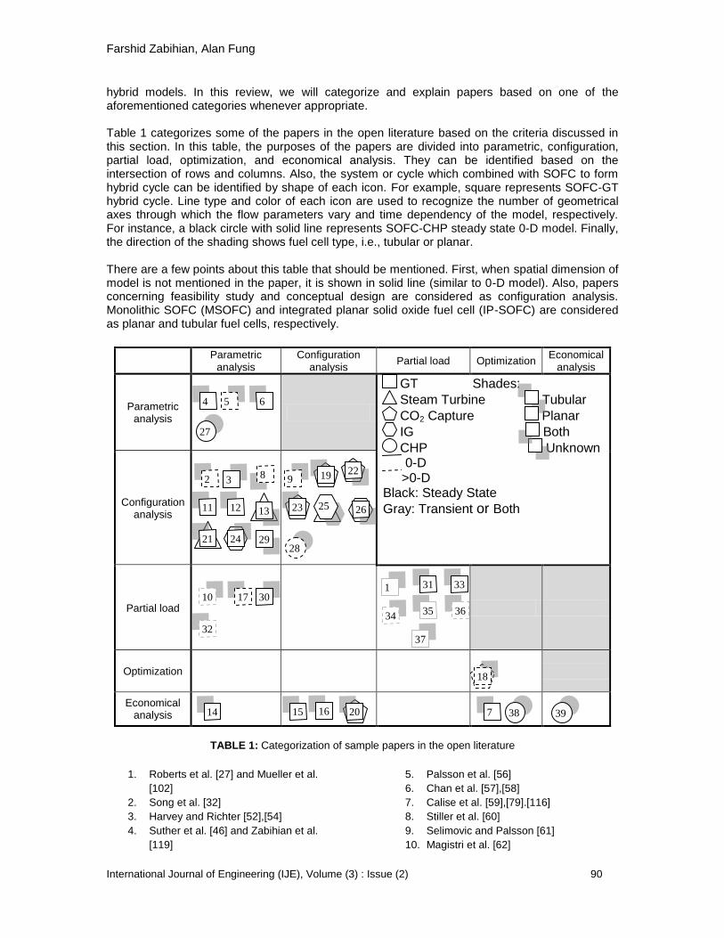
hybrid models. In this review, we will categorize and explain papers based on one of the aforementioned categories whenever appropriate. Table 1 categorizes some of the papers in the open literature based on the criteria discussed in this section. In this table, the purposes of the papers are divided into parametric, configuration, partial load, optimization, and economical analysis. They can be identified based on the intersection of rows and columns. Also, the system or cycle which combined with SOFC to form hybrid cycle can be identified by shape of each icon. For example, square represents SOFC-GT hybrid cycle. Line type and color of each icon are used to recognize the number of geometrical axes through which the flow parameters vary and time dependency of the model, respectively. For instance, a black circle with solid line represents SOFC-CHP steady state 0-D model. Finally, the direction of the shading shows fuel cell type, i.e., tubular or planar. There are a few points about this table that should be mentioned. First, when spatial dimension of model is not mentioned in the paper, it is shown in solid line (similar to 0-D model). Also, papers concerning feasibility study and conceptual design are considered as configuration analysis. Monolithic SOFC (MSOFC) and integrated planar solid oxide fuel cell (IP-SOFC) are considered as planar and tubular fuel cells, respectively.
Parametric
analysis Configuration
analysis Partial load Optimization Economical
analysis
Parametric analysis
GT Shades: Steam Turbine Tubular CO2 Capture Planar IG Both CHP Unknown 0-D >0-D
Black: Steady State Gray: Transient or Both
Configuration analysis
Partial load
Optimization
Economical analysis
TABLE 1: Categorization of sample papers in the open literature
1. Roberts et al. [27] and Mueller et al.
[102]
2. Song et al. [32]
3. Harvey and Richter [52],[54]
4. Suther et al. [46] and Zabihian et al.
[119]
5. Palsson et al. [56]
6. Chan et al. [57],[58]
7. Calise et al. [59],[79].[116]
8. Stiller et al. [60]
9. Selimovic and Palsson [61]
10. Magistri et al. [62]
1
7
10
15
16
17
14
31
33
32
30
37
35 36
34
18
20
39 38
27
2 3
4 5 6
8
9
11
12
13
19
21
23
22
24
25 26
28 29

Farshid Zabihian, Alan Fung
International Journal of Engineering (IJE), Volume (3) : Issue (2) 91
11. Granovskii et al. [63],[77],[80]
12. Pangalis et al. [65] and Cunnel et al. [66]
13. Kuchonthara et al. [67],[69]
14. Tanaka et al [68]
15. Lundbergm et al. [70]
16. Rao and Samuelsen [72]
17. Song et al. [73]
18. Möller et al. [75]
19. Riensche et al. [81]
20. Franzoni et al. [83]
21. Massardo et al. [84]
22. Inui et al. [85]
23. Campanari and Chiesa [86]
24. Lobachyov and Richter [88]
25. Kivisaari et al. [89]
26. Kuchonthara et al. [90]
27. Van Herle et al. [93]
28. Braun et al. [97]
29. Winkler and Lorenz [98]
30. Steffen et al. [99] and Freeh et al. [100]
31. Costamagna et al. [101]
32. Stiller et al. [104],[105],[110]
33. Chan et al. [107]
34. Zhang et al. [108]
35. Zhu and Tomsovic [109]
36. Kemm et al. [111]
37. Lin and Hong [112]
38. Riensche et al. [113],[114]
39. Fontell et al. [115]
5. MODELING STEPS
Before starting modeling of a hybrid system, it is very important to define what the purpose of desired model is and then to determine the key features of the model. The best modeling approach and the characteristics of the model depend on the application. Although this is a vital step, there is high tendency to be oversight. After finalizing these criteria, details of the model can be identified [7]. Similar to modeling of other thermal systems, the first step in the modeling of a SOFC hybrid system is to understand the system and translate it into mathematical equations and statements. The common steps for model development are as follows:
specifying a control volume around desired system,
writing general laws (including conservation of mass, energy, and momentum; second law of thermodynamics; charge balance; and so on),
specifying boundary and initial conditions,
solving governing equations by considering boundary and initial conditions (analytical or numerical solution),
validating the model. Although fuel cell simulation is a three dimensional and time dependent problem, by proper assumptions it can be simplified to a steady state, 2-D, 1-D, or 0-D problem for different applications and objectives [12]. As it will be shown later on, most of the SOFC hybrid system simulations in the open literature are 0-D models. In this type of modeling, series of mathematical formulations are utilized to define output variables based on input ones. In this approach, fuel cell is treated as a dimensionless box and that is why some authors referred it as box modeling. Despite the large numbers of assumptions and simplifications in this method, it is useful to analyze the effects of various operational parameters on the cycles overall performance, perform sensitivity analysis, and compare different configurations. When the objective of modeling is to investigate the inner working of SOFC, 0-D approach is not appropriate. However, for hybrid SOFC system simulation, where emphasize is placed on interaction of fuel cell and rest of the system and how fuel cell can affect the overall performance of the system, this approach can be suitable. In this level of system modeling, there are variety of assumptions and simplifications. For instance, Winkler et al. [23] developed a hybrid fuel cell cycle and assumed that the fuel cell was

Farshid Zabihian, Alan Fung
International Journal of Engineering (IJE), Volume (3) : Issue (2) 92
operated reversibly, representing any fuel cell type, and the heat engine was a Carnot cycle, representing any heat engine. Different software and programming languages have been used in hybrid SOFC systems simulation. Since there is no commercially available model for SOFC stack, all modelers should prepare their own model with appropriate details and assumptions. Therefore, from this point of view, what differentiates models is how they simulate the other components of the system. Generally, they can be divided into two categories. In the first approach, whole models can be developed in programming languages such as Fortran or high level software such as MATLAB/Simulink
® platform to solve governing equations of the system. In the second approach,
the modelers can take advantage of commercial software such as Aspen Plus® to model
conventional components of the cycle. These approaches will be discussed in detail later on. Due to the nature of numerical modeling, its results should be used carefully. In every modeling, the physical realities of the system should be translated into mathematical equations and solution of these equations is used to express behavior of the system. In case of fuel cells, the physical realities are extremely complex and some of which are completely unknown. Therefore, in order to extract these governing equations, high level of assumptions and simplifications should be considered which in turn introduce inaccuracy to the final results. This means fuel cell models are a “simplified representation of real physics” and even with appropriate validation accuracy of their results cannot be guaranteed [14]. For instance, one should be aware of the possible problems that can arise when local equations are considered as global. Bove et al. [39] highlighted such problem in their paper. They described the main problem of using 0-D approach for modeling was the negligence of variation in the fuel, air, and exhaust gas compositions through the fuel cell. As a consequence of this problem, when the inlet, outlet or an average value of the gas composition was used in the modeling, different results could be obtained. In particular, it was shown that it was impossible to evaluate effects of fuel utilization variation through the fuel cell when inlet gas composition was considered. On the other hand, considering output streams composition could result in underestimating cell voltage and power output. However, Magistri et al. [40] studied simplified versus detailed SOFC models and how this affected the predictions of the design-point performance of the hybrid systems. They emphasized the usefulness of the simplified model for hybrid system design and off-design analysis and detailed model for complete description of the SOFC internal behavior. More discussion and examples on this issue can be found in section “2-Dimentional models”. Judkoff and Neymark [41] classified the sources of simulation errors into three groups (these were provided for building simulation programs, but they were equally applicable to SOFC hybrid systems simulation):
Errors introduced due to assumptions and simplifications,
Errors or inaccuracies in solving mathematical equations,
Coding errors. They also proposed a pragmatic, three-step approach to identify these errors. In the first approach, comparative testing, the results of the model should be compared with the results of other models for the same problem with the similar initial and boundary conditions. If the results of the models match with acceptable error, it means the implementations are acceptable. However, this does not guarantee the correctness of the results because they all can be incorrect. In the second approach, analytical validation, the results of the model for a simple case are compared with the results of available analytical solution. Finally, in empirical validation the results of the simulation are compared with real data from the actual system under laboratory or field conditions.
Farshid Zabihian, Alan Fung
International Journal of Engineering (IJE), Volume (3) : Issue (2) 93
Finally, the validation of a model is important because a model must be validated to be a credible tool. Appropriate data are needed for validation. With limited resources, this can be difficult because most data cannot be found in the open literature. Although performance data from an entire hybrid power generation systems are usually proprietary and are not available in the literature, this information from single system is easier to find. Therefore, a way to resolve the problem of limited performance data is to develop and validate well defined sub-system models, and then integrate them to have a complete model of a large hybrid power generation system. Although SOFC is considered as the heart of these hybrid cycles, its detailed mathematical modeling and simulation methodology is not included in this review. The focus here is on the evaluation of overall system performance and not its components performance. One can refer to references [10, 11, 12, 13, 14] for review papers on SOFC modeling. In addition, some good examples of such simulations can be found in [42, 43] for steady state and [44, 45] for transient and dynamic modeling.
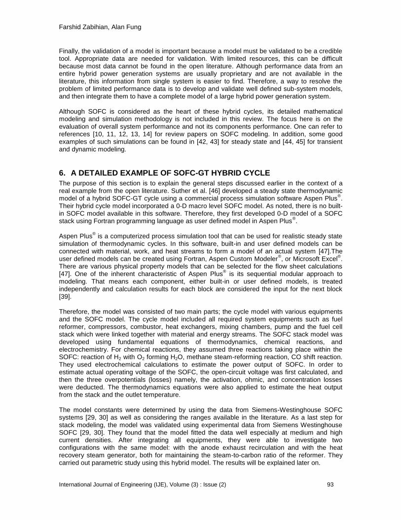
6. A DETAILED EXAMPLE OF SOFC-GT HYBRID CYCLE
The purpose of this section is to explain the general steps discussed earlier in the context of a real example from the open literature. Suther et al. [46] developed a steady state thermodynamic model of a hybrid SOFC-GT cycle using a commercial process simulation software Aspen Plus
®.
Their hybrid cycle model incorporated a 0-D macro level SOFC model. As noted, there is no built-in SOFC model available in this software. Therefore, they first developed 0-D model of a SOFC stack using Fortran programming language as user defined model in Aspen Plus
®.
Aspen Plus
® is a computerized process simulation tool that can be used for realistic steady state
simulation of thermodynamic cycles. In this software, built-in and user defined models can be connected with material, work, and heat streams to form a model of an actual system [47].The user defined models can be created using Fortran, Aspen Custom Modeler
®, or Microsoft Excel
®.
There are various physical property models that can be selected for the flow sheet calculations [47]. One of the inherent characteristic of Aspen Plus
® is its sequential modular approach to
modeling. That means each component, either built-in or user defined models, is treated independently and calculation results for each block are considered the input for the next block [39]. Therefore, the model was consisted of two main parts; the cycle model with various equipments and the SOFC model. The cycle model included all required system equipments such as fuel reformer, compressors, combustor, heat exchangers, mixing chambers, pump and the fuel cell stack which were linked together with material and energy streams. The SOFC stack model was developed using fundamental equations of thermodynamics, chemical reactions, and electrochemistry. For chemical reactions, they assumed three reactions taking place within the SOFC: reaction of H2 with O2 forming H2O, methane steam-reforming reaction, CO shift reaction. They used electrochemical calculations to estimate the power output of SOFC. In order to estimate actual operating voltage of the SOFC, the open-circuit voltage was first calculated, and then the three overpotentials (losses) namely, the activation, ohmic, and concentration losses were deducted. The thermodynamics equations were also applied to estimate the heat output from the stack and the outlet temperature. The model constants were determined by using the data from Siemens-Westinghouse SOFC systems [29, 30] as well as considering the ranges available in the literature. As a last step for stack modeling, the model was validated using experimental data from Siemens Westinghouse SOFC [29, 30]. They found that the model fitted the data well especially at medium and high current densities. After integrating all equipments, they were able to investigate two configurations with the same model: with the anode exhaust recirculation and with the heat recovery steam generator, both for maintaining the steam-to-carbon ratio of the reformer. They carried out parametric study using this hybrid model. The results will be explained later on.
Farshid Zabihian, Alan Fung
International Journal of Engineering (IJE), Volume (3) : Issue (2) 94
Next section will highlight very early modeling experience on SOFC hybrid cycles in the open literature.
7. EARLY MODELS
The SOFC development has started in the late 1950s, the longest continuous development period among various types of fuel cells [4]. However, it was not until the mid 1980s that results of first simple SOFC models were published in the open literature. For SOFC hybrid cycle, the first papers were being published in early 1990s. Dunbar and Gaggioli have been considered as pioneers in the field of SOFC modeling and their integration with Rankine cycle. They published their first paper on the results of mathematical modeling of the performance of solid electrolyte fuel cells as early as 1988 [48]. In 1990 [25], they proposed integrating SOFC units into a conventional Rankine steam cycle power plant. That study revealed significant efficiency increase, up to 62%, compared to the maximum conventional plant efficiency of about 42% in those days [25]. They found that the main reason for this efficiency improvement was higher exergetic efficiency of SOFC as contrasted with the combustion process in conventional fossil fuel fired power plants [49]. They also investigated [50] the exergetic effects of the major plant components as a function of fuel cell unit size. The results showed that specific fuel consumption might be reduced by as much as 32% in hybrid cycle. Harvey and Richter, who proposed a hybrid thermodynamic cycle combining a gas turbine and a fuel cell, are the pioneers in this area. Harvey et al. [51] first proposed the idea in 1993 by conducting one of the earliest modeling works in SOFC-GT hybrid cycle. They developed a model [52] to simulate monolithic SOFC (MSOFC) combined with intercooled GT in Aspen Plus
® and a
fuel cell simulator developed by Argonne National Laboratory [53]. They found that for a power
plant with net electricity generation of 100 MW, about 61 MW were produced by the SOFC with
the thermal efficiency of 77.7% (lower heating value, LHV). In addition their second law analysis noted the large exergy destruction in SOFC, combustor, and air mixer. They concluded that internal reforming could improve both system efficiency and its simplicity. In their following paper [54], they improved the model by incorporating internal reformer to the cycle and taking into account all major cycle overpotentials. This time the cycle efficiency was 68%. Moreover, they noted that the system efficiency increased with cycle pressure. They determined that maximum efficiency could be achieved at system operating pressure equal to 15 bar while satisfying the system constraints. They also compared efficiency of cycle with internal and external reforming and surprisingly found that their efficiencies were almost identical. The thermodynamics second law analysis showed that exergy destructions in internal reforming cycle were marginally higher than those of external reforming cycle (275 versus 273 MJ/s). For the successful integration of the SOFCs with other power generating technologies such as gas turbines, models that can accurately address steady state and dynamic behavior of systems with different configurations, optimization, fluctuating power demands and techno-economic evaluation are required. In the next sections, models that addressed these objectives will be discussed.
8. PARAMETRIC STUDIES
One of the primary aims of any system simulation is to evaluate the effects of various parameters on system performance. By doing so, the most influential parameters can be identified. In turn, these parameters should be considered for system optimization within system constraints.

Farshid Zabihian, Alan Fung
International Journal of Engineering (IJE), Volume (3) : Issue (2) 95
The curves in Figure 1 are presented to quickly summarize the results of these parametric studies in the literature. For instance, if a performance parameter is linearly increasing, Curve 2 will be referred to describe the trend [55].
FIGURE 1: Performance parameter symbolic curves [55].
The first study to be reviewed in this section is presented by Suther et al. [46]. The model has already been explained in “A detailed example of SOFC-GT hybrid cycle” section. They studied the effects of system pressure, SOFC operating temperature, turbine inlet temperature (TIT), steam-to-carbon ratio (SCR), SOFC fuel utilization factor, and GT isentropic efficiency on the specific work output and efficiency of two generic hybrid cycles with and without anode off-gas recirculation. They chose specific work output (actual work divided by air mass flow rate) and cycle efficiency as two main performance parameters. The high specific work output was preferred because it meant lower air flow rate was required for the same system power output, which translated into smaller equipments. They found cycle specific work and thermal efficiency with respect to system parameters to follow curves in Figure 1 as follows:
Specific work and efficiency with respect to system pressure followed Curve 4 and Curve 5 for system with anode off-gas recirculation and Curve 4 and Curve 2 for system without anode off-gas recirculation, respectively.
Specific work and efficiency with respect to SOFC operating temperature followed Curve 3 and Curve 2, respectively, for both systems with and without anode off-gas recirculation.
Specific work and efficiency with respect to TIT followed Curve 2 and Curve 3, respectively, for both configurations.
Specific work and efficiency with respect to SOFC current density followed Curve 3 for both configurations.
Specific work and efficiency with respect to SCR followed Curve 2 and Curve 3, respectively, for both configurations.
Specific work and efficiency with respect to SOFC fuel utilization factor followed Curve 5 and Curve 2 or 3 (depending on GT isentropic efficiency), respectively, for both configurations.
The results showed that the cycle efficiencies with and without anode off-gas recirculation were very close with variation in many of the system parameters. Palsson et al. [56] developed a steady state model for a combined SOFC-GT system featuring external pre-reforming and recirculation of anode gases in Apsen Plus
® by using their SOFC

Farshid Zabihian, Alan Fung
International Journal of Engineering (IJE), Volume (3) : Issue (2) 96
model as a user defined unit and other components modeled as standard unit operation models. In order to model SOFC, they used 2-D model of planar electrolyte-supported SOFC. The finite volume method was used to discretize cell geometry by considering resistance and activation polarisation. Their system size was 500 kW because they believed this was proper size for demonstration and market entry purposes. It should be noted that they added primary fuel to increase TIT but they maintained fuel flow to the system constant. Furthermore, in order to provide heat for district heating system, they added a cooler to cycle exhaust stream. This simple cooler limited the exhaust temperature to a specific value (80 ºC). They studied various system parameters, including the electrical efficiency, specific work, TIT, and SOFC temperature with respect to the pressure ratio. Their sensitivity studies revealed that these parameters varied according to Curve 6, Curve 4, Curve 2, and Curve 1, respectively. Moreover, the electrical efficiency and SOFC temperature varied with respect to the cycle inlet air flow rate according to Curve 3 and Curve 2, respectively. They found that increasing TIT did not improve system efficiency and specific work. Because in order to increase TIT, more fuel should be combusted at GT combustion chamber, thus less fuel remained to be consumed in SOFC unit. Their analysis showed that system operating pressure had great impact on hybrid system performance. At lower pressure ratios (PRs), the efficiency increased slightly to an optimum point and then sharply decreased for higher PRs. A maximum efficiency of 65% could be achieved at a pressure ratio of 2. At this point the GT output was almost zero; therefore, this efficiency was equal to SOFC efficiency. The slight improvement in system efficiency stemmed in increased efficiency of SOFC. At higher PRs, more power output from the gas turbine and less from the SOFC decreased system overall efficiency. In addition, they pointed out that cell voltage had no impact on system performance. Similarly, they investigated the performance improvement of the system when the intercooling of air compressor and gas turbine reheat were added and found that their application would not be worthwhile because of their relatively small impact, particularly for the reheat case. The discrepancy between the results of Suther et al. [46] and Palsson et al. [56] is due to the different control strategies of the two systems. In the former, the fuel flow was kept constant when varying the system operating pressure. But in latter, as mentioned earlier in this section, although the total fuel flow rate was held constant, part of this fuel fed to the gas turbine combustor to sustain the turbine exhaust temperature in specified range. Therefore, in the case of Palsson et al. [56], at high system operating pressures more fuel combusted in the GT combustor resulting in more work to be generated in GT at lower efficiency, which in turn lowered cycle overall efficiency. Chan et al. [57, 58] developed a model of simple SOFC-GT-CHP power system and performed the first law of thermodynamics energy analysis on the model. Their model achieved electrical and total efficiencies of over 62% and 83%, respectively. Then, they investigated the effects of system operating pressure and fuel flow rate on the system overall performance. They showed that system efficiency with respect to pressure and fuel flow rate followed Curve 2 and 3, respectively. Their results and Palsson et al. [56] results do not show the same trend. The reason is similar to what was explained in previous paragraph. Calise et al. [59] investigated the impacts of current density, system operating pressure, fuel-to-oxygen ratio, water-to-methane ratio, and fuel utilization factor on the electrical efficiency of a hybrid SOFC-GT system and found the electrical efficiency to follow Curve 3, Curve 4, Curve 4, Curve 1, and Curve 2, respectively, when varying these parameters. They also showed that increasing the fuel utilization factor of SOFC could slightly improve cycle performance. In contrast with the fuel utilization factor, the effect of SCR was not favorable. It was stated that this was as a results of more energy being used to generate steam in heat recovery steam generator and less energy for power generation. These results are in agreement with Suther et al. [46] results.
Farshid Zabihian, Alan Fung
International Journal of Engineering (IJE), Volume (3) : Issue (2) 97
9. 2-DIMENSIONAL MODELS
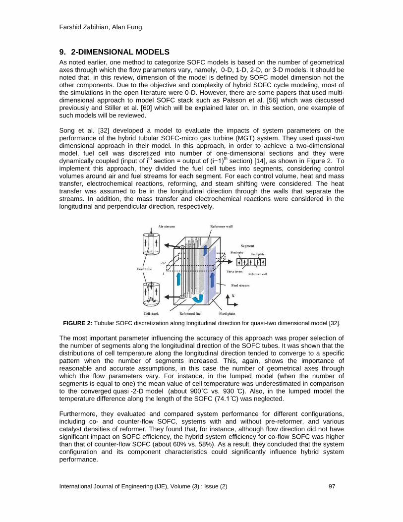
As noted earlier, one method to categorize SOFC models is based on the number of geometrical axes through which the flow parameters vary, namely, 0-D, 1-D, 2-D, or 3-D models. It should be noted that, in this review, dimension of the model is defined by SOFC model dimension not the other components. Due to the objective and complexity of hybrid SOFC cycle modeling, most of the simulations in the open literature were 0-D. However, there are some papers that used multi-dimensional approach to model SOFC stack such as Palsson et al. [56] which was discussed previously and Stiller et al. [60] which will be explained later on. In this section, one example of such models will be reviewed. Song et al. [32] developed a model to evaluate the impacts of system parameters on the performance of the hybrid tubular SOFC-micro gas turbine (MGT) system. They used quasi-two dimensional approach in their model. In this approach, in order to achieve a two-dimensional model, fuel cell was discretized into number of one-dimensional sections and they were dynamically coupled (input of i
th section = output of (i−1)
th section) [14], as shown in Figure 2. To
implement this approach, they divided the fuel cell tubes into segments, considering control volumes around air and fuel streams for each segment. For each control volume, heat and mass transfer, electrochemical reactions, reforming, and steam shifting were considered. The heat transfer was assumed to be in the longitudinal direction through the walls that separate the streams. In addition, the mass transfer and electrochemical reactions were considered in the longitudinal and perpendicular direction, respectively.
FIGURE 2: Tubular SOFC discretization along longitudinal direction for quasi-two dimensional model [32].
The most important parameter influencing the accuracy of this approach was proper selection of the number of segments along the longitudinal direction of the SOFC tubes. It was shown that the distributions of cell temperature along the longitudinal direction tended to converge to a specific pattern when the number of segments increased. This, again, shows the importance of reasonable and accurate assumptions, in this case the number of geometrical axes through which the flow parameters vary. For instance, in the lumped model (when the number of segments is equal to one) the mean value of cell temperature was underestimated in comparison to the converged quasi -2-D model (about 900 ̊C vs. 930 ̊C). Also, in the lumped model the temperature difference along the length of the SOFC (74.1 ̊C) was neglected. Furthermore, they evaluated and compared system performance for different configurations, including co- and counter-flow SOFC, systems with and without pre-reformer, and various catalyst densities of reformer. They found that, for instance, although flow direction did not have significant impact on SOFC efficiency, the hybrid system efficiency for co-flow SOFC was higher than that of counter-flow SOFC (about 60% vs. 58%). As a result, they concluded that the system configuration and its component characteristics could significantly influence hybrid system performance.

Farshid Zabihian, Alan Fung
International Journal of Engineering (IJE), Volume (3) : Issue (2) 98
10. MODELS FOR COMPARISON OF CONFIGURATIONS
As stated, an important objective of hybrid SOFC systems modeling is to predict system performance for different configurations. There have been huge number of proposed hybrid SOFC systems in the open literature that combined SOFC stacks with heat exchangers, compressors, GTs, pre-reformers, mixers, heat recovery steam generators (HRSGs), CO2 capture, combustors and so on (such as Campanari et al. [28]). However, there have been no universally accepted configuration(s) yet and scientists are still trying to propose innovative cycles for the SOFC hybrid systems. In this section, various configurations proposed in the open literature for stack and equipments will be reviewed. Stiller et al. [60] developed 2-D planar and 1-D tubular SOFC models to simulate SOFC-GT hybrid cycle. They investigated effects of different parameters such as pressure ratio, air inlet temperature and so on to compare performance of two cycles. It was shown that hybrid systems could achieve efficiencies above 65% with both planar and tubular SOFC. The main difference between the planar and the tubular SOFC cycles was the internal pre-heating of the air in the tubular system which allowed a lower air inlet temperature to the stack. This reduced the amount of required high temperature heating in the pre-heating. This effect was compensated by lower efficiency of the tubular fuel cell stack, due to its higher ohmic loss. Selimovic and Palsson [61] investigated the effect of networked SOFC stacks, i.e., using two smaller stacks in series (in terms of fuel and air flow) instead of conventional one stage stack. They used same model as [56], with minor modifications. They showed that for a stand-alone SOFC, fuelled by hydrogen or 30% pre-reformed methane, dividing the single stage stack into two smaller stacks in series (staged stacks) increased the power output by 2.7% and 0.6%, respectively. The reason stemmed in increased uniformity of current density in staged system. Then, they examined SOFC-GT hybrid cycle fuelled by natural gas (NG) for two options, both the air and fuel stream in series (network A) or only the fuel stream in series and air stream divided (network B). The results signified that there was 4.7% points performance improvement in network A, whereas efficiency was reduced by 1.5% points for network B. They concluded that for relatively small stacks, networked stacks could reduce cooling demand of the cells, so they were preferred. Magistri et al. [62] developed a model to investigate the performance of a hybrid system consisting of integrated planar SOFC (IP-SOFC), GT, and district heating. They found that overall efficiency of atmospheric hybrid system was 10% lower than that of pressurized system. In 2007, Granovskii et al. [63] presented results of their simulation of combined SOFC–GT system for two possible configurations to provide required steam-to-methane ratio (in all cases higher than 2 [64]), cycle with anode exhaust recirculation and cycle with HRSG for steam generation. They also added a Rankine steam cycle at the bottom of GT for the configuration with anode exhaust recirculation. They preformed energy and exergy analysis on the models and determined that the suitability of these schemes depended on the application of the power generation system. For example, although configuration with anode off-gas recycle had higher exergy and energy efficiencies, the other scheme was associated with a higher power generation capacity. Pangalis et al. [65] and Cunnel et al. [66] modeled and compared six different configurations of hybrid SOFC-GT systems by considering variety of features in each system, including combustion chamber, recuperator, intercooler, and reheat SOFC stack. They showed that both thermal efficiency and net specific power versus compression ratio for most of the configurations followed Curve 4. They found that the optimal configuration in terms of efficiency could be achieved when GT with intercooler and recuperator were integrated to primary SOFC (ahead of the combustor) and reheat SOFC (between high- and low- pressure GT) with efficiency of 76%. Also, they showed that in configuration with intercooler and recuperator integrated to primary SOFC, the net specific power was maximized. Again, they concluded that the most important
Farshid Zabihian, Alan Fung
International Journal of Engineering (IJE), Volume (3) : Issue (2) 99
factor for selecting hybrid SOFC system configuration was the application of power plant. For example, recuperated GT with SOFC ahead of combustor with thermal efficiency of 64% at relatively low pressure ratio of 14 and the specific power of 520 kW/kg was probably the most suitable configuration for small and medium scale power generation. Kuchonthara et al. [67] developed their hybrid SOFC model by writing a Fortran code for SOFC and running it in Aspen Plus
®. They conducted a parametric analysis on two hybrid SOFC system
configurations: hybrid SOFC-GT with heat recuperation (HR) system and hybrid SOFC-GT with heat and steam recuperation (HSR) system. In the former, heat from the GT exhaust was recovered by an air preheating system whereas, in latter, an air preheating system and a HRSG were used for this purpose. In HSR system, in order to increase net mass flow and power output of GT, the generated steam was directly injected into the combustor. They found that GT power output and system overall thermal efficiency were higher in HSR configuration, due to higher energy recuperation rate in this configuration. Also, they illustrated that higher pressure ratios increased the synergetic effect of steam recuperation. Furthermore, their parametric analysis showed that the SOFC work, GT work, TIT, and thermal efficiency with respect to the SOFC fuel utilization factor varied according to Curve 2, Curve 3, Curve 3, and Curve 4, respectively. Also, the cycle specific work and thermal efficiency with respect to the TIT followed Curve 5 and Curve 6, respectively. They evaluated the overall efficiency of the cycle against TIT for different pressure ratios (PRs). They found that, at low TITs, the thermal efficiency decreased when pressure ratio increased. This was due to lower fuel utilization factor in SOFC for higher PRs. In contrast, higher PRs led to thermal efficiency improvement at high TITs due to larger GT power output. It seemed that their results completed previous studies [46, 56, 68] on the effect of TIT on cycle’s overall performance. As a result, they suggested that optimal system (both high power output and high efficiency simultaneously) could be achieved when system operated at high TIT with an optimal pressure ratio. Similarly, they published another paper [69] to evaluate performance of hybrid systems when SOFC cycle integrated with various enhanced gas turbine cycles namely, steam injected gas turbine (STIG) cycle (including additional air preheating), GT-steam turbine (ST) combined cycle, and humid air turbine (HAT). They assessed effects of operating conditions, such as TIT and PR, on the overall efficiency and specific work output of the system. They concluded that SOFC–HAT system, operating at high TIT and PR, not only could significantly improve system performance, but also could lessen the problem of water supply by reducing water consumption. One of the challenges in SOFC hybrid systems development is to find a gas turbine that matches the requirements of hybrid cycle. Lundbergm et al. [70] studied the possibility of 20 MW-class hybrid system that integrated a pressurized SOFC with a Mercury 50 gas turbine. The Mercury 50 was chosen due to its unique characteristics, including high thermal efficiency, power rating, modular design, reliability, and low cost of maintenance. They determined the optimal size of pressurized SOFC (PSOFC) in a hybrid system with a single Mercury 50 gas turbine using the cost of electricity (COE) as the optimizing parameter. Minimum COE was achieved when four PSOFC modules and one Mercury 50 gas turbine were integrated to generate approximately 12.5 MW at an efficiency of nearly 60% (Net AC/LHV). They also explained the required modification on commercially available GTs. Furthermore, they studied different bottoming cycle options (combined cycle power plant and ammonia-water cycle) to utilize thermal energy at GT exhaust. On the other hand, most of the works performed on the modeling of hybrid SOFC and GT concentrated on the fuel cell operation using the performance characteristics of existing GTs. However, different operating conditions of GT (i.e., the increased pressure losses) in hybrid cycle shifts the operating point of compressor and GT to an off-design areas. Sieros and Papailiou [71] examined the optimal fitting of a small GT in a hybrid SOFC-GT for both design-point and part-load operation conditions. They proposed variable geometry components, namely variable nozzle turbine and variable diffuser compressor to avoid compressor surge and increase part-load

Farshid Zabihian, Alan Fung
International Journal of Engineering (IJE), Volume (3) : Issue (2) 100
efficiency. They concluded that further work should be performed for the detailed design of these devices. Rao and Samuelsen [72] introduced SOFC cycle coupled with intercooled-reheat GT as reference power generation system for their thermodynamic modeling. Then, they formed their alternative cases by incorporating HAT system to their reference case and also replacing reheater with second SOFC (dual SOFC-HAT). They found that efficiency of the reference case and its alternatives were 66%, 69%, and 76%, respectively. In addition, they showed that the second scenario could achieve lowest cost of electricity (COE). Song et al. continued their previously explained work [32] in another research [73]. They extended their model to find optimal matching between a commercially available GT (Mercury 50) and a SOFC unit. The parameters to be matched were included: operating temperature, pressure and operating strategies and maximum allowable cell temperature as a limiting parameter. Based on the selected condition, the total system power at design-point condition was 11.5 MW at a system efficiency of about 59%. In comparison to the power ratio of SOFC and GT in kW-class cases described in Veyo et al. [30], the power ratio of this system was very low. Their results agreed with results found by Lundbergm et al. [70].
11. OPTIMIZATION
A quick survey of the literature in the modeling of hybrid SOFC systems shows that little has been done for optimization of these systems. In most of those few works, such as [74], sensitivity analysis of various parameters was preformed to develop an optimal SOFC hybrid power generation system. However, due to the large number of parameters involved and complex nature of their interrelation and correlation, suitability of this optimization method is controversial. In optimization of a typical SOFC hybrid cycle 5 to 10 (or even more) [75] independent variable should be considered, depending on how complex the system and model are. Therefore, it is vital to seek for methods that can optimize these non-linear multi-dimensional systems [75]. In a considerable development in the optimization of SOFC-GT systems, Möller et al. [75] deployed genetic algorithm (GA) to optimize SOFC-GT configuration with and without a CO2 separation plant. In order to model the SOFC stack, they used the same model as in [56]. In their optimization, the electrical efficiency was selected as the objective function. Also, the air flow, fuel flow, cell voltage in the stack, air temperature at the stack inlet, reformer duty, and pressure ratio were selected as decision parameters. The optimization procedure resulted in a SOFC-GT system with above 60% efficiency when equipped with CO2 capture. The results showed that the system efficiency was greatly influenced by SOFC temperature. Furthermore, a low air flow and no or little supplementary fuel could improve the system efficiency.
12. EXERGY ANALYSIS
According to Dincer and Rosen [76] exergy analysis is a method that can be applied to design, improve, and analyze the energy systems. This technique considers the second law of thermodynamic as well as the conservation of mass and energy, simultaneously. Granovskii et al. [77] evaluated the importance of exergy analysis in applying the “principles of industrial ecology” for integrating different technologies. For instance, they preformed exergy analysis on a SOFC-GT hybrid system and found that the depletion number of standalone SOFC and GT were much higher than that of hybrid system. This confirmed that the SOFC-GT hybrid system was more environmentally friendly. The depletion number, proposed by Connelly and Koshland [78], is a concept to describe the efficiency of fossil fuel consumption according to exergy analysis and is defined based on how exergy destruction within a system is related to total exergy input.
Farshid Zabihian, Alan Fung
International Journal of Engineering (IJE), Volume (3) : Issue (2) 101
Calise et al. in previously mentioned paper (in parametric studies section) [59] and their other paper [79] (with a few changes in system configuration) preformed the second law of thermodynamics analysis on a gas turbine cycle integrated with SOFC. Their exergy analysis illustrated that the SOFC stack and the catalytic burner were responsible for most of exergy destruction, respectively, when the hybrid system operated at design-point. This high rate of exergy destruction stemmed in inefficiencies of chemical reactions occurring in those equipments. Despite the high efficiency of SOFC, fuel cell stacks are the greatest source of exergy losses due to the number of chemical and electrochemical reactions, such as steam reforming and electrochemical oxidation, taking place simultaneously. Similarly the catalytic burner, where anode off-gas stream was combusted, demonstrated a significant exergy destruction rate. On the other hand, exergy destruction rate of turbomachineries were not remarkable because of their high isentropic efficiencies and low energy flows. They also preformed exergy analysis on partial load operation and found that although exergy destruction generally increased, its rate depended on the selected control scheme. Finally, they concluded that in hybrid energy systems design, particular emphasizes should be placed on component with highest exergy losses, i.e. SOFC stacks. In their other paper, Granovskii et al. [80] presented exergetic performance analysis of a SOFC-GT hybrid cycle. They found that the SOFC stack and the combustion chamber were the components with highest rate of exergy destruction, respectively, similar to results of Calise et al. But in their model the difference in exergy losses of SOFC stack and combustion chamber was less than 5%.
13. CO2 CAPTURE
Although SOFC hybrid power plants are considered to be the cleanest technology to generate electricity from fossil fuels (due to their high efficiency and minimal fuel combustion), still there is considerable amount of CO2 in their exhaust. Therefore, integrating CO2 separation technologies to SOFC hybrid plants is an active field of research. In this section, some of the models for such plants will be discussed. In 1999 Riensche et al. [81] developed a model to simulate a near zero CO2 emission hybrid SOFC-GT power plant. Their adiabatic tubular air electrode supported fuel cell model was based on one of the earliest planar SOFC model [82]. There are two approaches to separate CO2 in the exhaust stream of power plants. In one of these approaches, the spent fuel is combusted with pure oxygen, instead of air, to avoid introducing nitrogen to the plant’s off-gas stream. In their proposed model, they made use of one of the unique characteristics of SOFC cycle that other technologies cannot easily compete. They modeled a bank of oxygen ion conducting tubes (very similar to SOFC tubes) and passed the unused fuel over them. They found that system operation was optimal when the system was pressurized. It was concluded that a gross electric efficiency of about 50% to 60% for the tubular SOFC and 60% to 70% for the SOFC-GT combination were achievable in this configuration. Franzoni et al. [83] developed a model to simulate 1.5 MW SOFC-GT hybrid system based on the model explained in [84]. They compared performance of the hybrid plant when it was integrated with two CO2 capture technologies, namely fuel treatment and then separation of CO2 in exhaust by chemical absorption and combustion of spent fuel with pure oxygen. In the former approach, they observed 17% efficiency penalty, from 62% to 45% with 0.15 kgCO2/kWh of CO2 in exhaust. In second approach, the system was equipped with an air separation unit to provide oxygen for GT combustor. The efficiency loss in this case was much lower at 3.6% with near-zero CO2. The thermoeconomic analysis showed that the cost of second plant was significantly lower. With the same method, Inui et al. [85] used second approach (pure oxygen as the oxidant gas in GT combustion chamber) for CO2 capture. They found that the efficiency of cycle could reach as
Farshid Zabihian, Alan Fung
International Journal of Engineering (IJE), Volume (3) : Issue (2) 102
high as 71% (LHV) indicating that the proposed system could satisfy both expectations of high efficiency and ultra clean power generation. Campanari and Chiesa [86] compared performance of SOFC-GT cycle with two configurations for CO2 capture process. In the first scheme, steam and CO2 in the anode exhaust was separated by condensation and chemical absorption, respectively. Then, 30% of remaining fuel combusted in GT combustor and the rest was recycled to anode to be consumed in SOFC. In second scheme, CO in anode exhaust was converted to H2 in shift reactor. Then, existing CO2 was chemically absorbed, and hydrogen rich gas combusted in GT combustion chamber. The SOFC model for this plant was explained in [87]. The results showed that both plants exceed 71% (LHV) efficiency and removed 90% of CO2 in exhaust stream. Although utilization of the shift reactor increased complexity of second scheme, it took advantage of more desirable GT to SOFC power output ratio (0.29 vs. 0.20), a lower consumption of the auxiliaries (5.5% vs. 8.2% of the net output), and better potential to increase CO2 sequestration.
14. FUEL FLEXIBILITY
So far, in all models either natural gas or hydrogen has been considered as fuel. However, SOFC hybrid systems enjoy the advantage of being able to utilize other fuel sources. In this section, some models that use coal and biogas as fuel will be discussed. In one of the earliest works in this field, Lobachyov and Richter [88] presented results of their theoretical study on the system that incorporated a coal gasification process into hybrid SOFC-GT cycle, which the latter was proposed by Harvey and Richter [52]. They suggested recycling of part of the hot cathode off-gas to provide the heat required for gasification. They preformed energetic and exergetic analysis on the model. They found that the cycle could achieve up to 60% efficiency (energetic). Exergy analysis revealed that the gasifier, SOFC, and steam generator were responsible for most of exergy destruction. In addition, the integration of a two-stage GT with reheater and steam turbine at the bottom of GT resulted in 0.5% and 3.2% improvement in the system overall efficiency, respectively. Kivisaari et al. [89] preformed a feasibility study for integration of a high temperature fuel cell (either MCFC or SOFC), a gas production unit based on coal gasification and an existing networks of heat distribution among residential users (CHP plant). They considered a thermal input of 50 MW with and without anode off-gas recirculation for SOFC. They employed a one-point model to reduce calculation times and model complexity. They found that the introduction of the anode off-gas recirculation resulted in 12% increase of the power output from the SOFC because of the almost 10% increase in overall fuel utilization. These values, however, could not be trusted because their one-point model did not consider reduction in the concentration of the reacting streams. They observed that the final system, which was a combination of a gasifier, a standard low temperature gas cleanup and SOFC, could achieve an electrical and overall efficiency of about 47% and 85%, respectively. Another study on combination of coal gasification and fuel cell for power generation was presented by Kuchonthara et al. [90]. They considered the integrated power generation cycle combining with thermochemical recuperation, brown coal gasification and a SOFC. In order to model SOFC they used the same model as in [67, 69]. Their simulation indicated that the cycle efficiency could be increased from 39.5% (higher heating value, HHV) without the SOFC to about 45% with the SOFC. Rao et al. [91] performed thermoeconomic analysis of integrated gasification fuel cell (IGFC) plant and compared it with an integrated gasification combined cycle (IGCC). They showed that the cost of electricity of IGFC plant was compatible with that of the IGCC plant (based on $400/kW installation cost for SOFC stack).

Farshid Zabihian, Alan Fung
International Journal of Engineering (IJE), Volume (3) : Issue (2) 103
Sucipta et al. [92] used similar model as Song et al.’s [32] and added different biomass gasification processes, namely, air-, oxygen- and steam-blown, to analyze the effect of biomass fuel composition on SOFC-GT performance. They found that efficiencies level for all three cases were reasonably high (although lower than the reference case fueled with pure methane) and concluded that the biomass fueled SOFC–MGT hybrid system was suitable alternative for conventional power plants. They pointed out that air- and steam-blown biomass fuel had the lowest and highest efficiency, respectively, for both SOFC module and for the entire hybrid system. Van Herle et al. [93] performed the energy balance analysis on an existing biogas production unit, equipped with a 1 kW SOFC demonstrational stack as a small CHP system. The fact that they used some real data for their model and, to some extent, compared the results with measurement from the site made this paper among a few exceptions in this respect. They achieved almost 34% and 58% electrical and cogeneration thermal efficiency, respectively. The results were validated by the natural gas fueled Sulzer Hexis 1 kW systems with an electrical efficiency of 35% (direct current (DC), LHV) [94].They also compared two reformer technologies, i.e., steam reforming and partial oxidation reforming with air (POX). They also investigated the impacts of water addition for steam reforming process and observed that cogeneration thermal efficiency significantly decreased with water addition. This was due to the fact that there was no condensation in the exhaust to recover the evaporation heat consumed at the inlet. They assessed electrical and total efficiency of the system as a function of operating parameters such as CO2 fraction in the biogas feed, reforming conditions, air excess rate, SOFC stack temperature (followed Curve 4 and 5, respectively), and pressure (followed Curve 3 and 2, respectively). They showed the variation in electrical efficiency, when varying the CO2 fraction in the biogas feed between extreme composition limits. Probably unexpectedly, they stated that efficiency increased when more methane was replaced by carbon-dioxide. In other words, the system performance improved when fueled with poorer biogas (richer in CO2). They explained that higher methane content in inlet biogas fuel resulted in higher input LHV, which led to higher current, thus to higher ohmic overpotential and lower SOFC operating voltage. They also indicated that electrical efficiency reduced when system was pressurized. Clearly, this was in contrast with other studies such as Suther et al. [46] and Chan et al. [57]. The reason could be explained based on the fact that their model did not consider two positive impacts of higher system operating pressure: more work output when high pressure hot exhaust passed through GT and improved mass transfer which led to lower electrode overpotentials. Whereas, more compression work to pressurize inlets streams reduced net work output.
15. DIFFERENT APPLICATIONS (NON-STATIONARY ELECTRICTY GENERATION)
Stationary power generation plants are not the only application of SOFC hybrid cycles. The residential CHP, mobile application, and auxiliary power unit for vehicles and aircrafts are considered as potential applications of SOFC hybrid cycles. In this section a few simulations that addressed these applications will be presented. Nowadays, distributed generation (DG) of combined heat and power (CHP) cycles are gaining increasing attentions. This is due to the deregulation of the electricity market and widespread residential utilization of natural gas as a primary energy source. Although some authors proposed application of PEMFC for CHP application [95, 96], SOFC hybrid cycles are the most promising candidates in this field. Braun et al. [97] developed a model to evaluate the energetic and exergetic performance of various configurations of residential-scale SOFC-CHP hybrid system, including hydrogen- and methane-fueled systems with external and internal catalytic steam reforming, and cathode and

Farshid Zabihian, Alan Fung
International Journal of Engineering (IJE), Volume (3) : Issue (2) 104
anode off-gas recirculation. They investigated the parameters influencing suitability of this system to match residential demands and found that one of the most important parameters was the thermal-to-electrical load ratio (TER) of residential unit. TER defined as the ratio of the thermal energy demand of the home to its base electrical load. Their results indicated that the optimal system included cathode and anode off-gas recirculation and internal reforming of methane. The electrical and combined heat and power efficiencies of this system were 40% and 79% (HHV), respectively. In 2002, Winkler and Lorenz [98] investigated the potential utilization of SOFC-GT in mobile application. They first proposed a reheat SOFC-GT with the efficiency of more than 70%. They also showed that by incorporating a bottoming steam cycle to a reheat SOFC-GT hybrid system, the electrical efficiency of more than 80% could be possible. They illustrated that the electrical efficiency with respect to the SOFC pressure followed Curve 4. Their results well agreed with results of Yi et al. [74] and Suther et al. [46]. Finally, they investigated possibility of deployment of SOFC-GT in a mid-size car with capacity of 75 kW and efficiency of 55%. They concluded that the results of their modeling proved the feasibility of utilization of the SOFC–GT hybrid system in unconventional applications which required further and more detailed investigations. Steffen et al. [99] developed a model of SOFC-GT cycle to provide auxiliary power for a 300 passengers commercial transport aircraft in 2015. They stated that 440 kW was an adequate unit size for this application. Unlike the ground stationary power plants, in aerospace systems, power density (power/volume) and system specific power (power/mass) were the most important parameters to consider. Another remarkable difference in this application was fuel source which was jet fuel. This led to using catalytic partial oxidation (CPOX) for fuel reforming process. Their proposed system resulted in efficiency of about 63% (LHV) which was significantly higher than the efficiency of conventional systems at about 42%. However, the proposed system was much heavier (1396 kg versus 331 kg) mainly because of the metallic interconnect mass in fuel cell stack. They suggested that by applying some innovative techniques (e.g. corrugated flow channels) the system’s mass could considerably be reduced. They completed this study in another paper [100] by considering system partial load operation. In this case, system total mass increased considerably to 1912 kg.
16. TRANSIENT AND OFF-DESIGN CONDITION MODELING
In every energy system, dynamic and part-load behavior and load following characteristic are critical factors to consider. This is especially important for SOFC hybrid systems since they have been considered as forerunner technology in the market of distributed and residential power supply and mobile applications. Since these types of power stations operate in isolated condition, their load demand following characteristic is extremely important. Thus, part-load performance, operational stability and safety are key issues that should be addressed for SOFC based energy systems before they can be commercialized. The main objective of these studies is to design a control strategy that can maintain SOFC and GT inlet temperatures during load changes [27]. These aspects of SOFC hybrid system have been studied extensively in the literature. In this section some of these papers will be reviewed. Costamagna et al. [101] evaluated design and off-design performance of SOFC and MGT hybrid system. For design-point operation, they found the overall efficiency to be higher than 60% and MGT-to-SOFC work output ratio to be 0.19. In off-design operation, they considered two control strategies: constant and variable turbine rotational speed. In former scheme, the load was controlled by varying the overall fuel flow which resulted in the reduced system efficiency (from efficiency of 61% to 56% at 70% of the power at design-point). The latter involved variation of the MGT rotational speed. However, operation mode of conventional large size GT plants generally did not provide such opportunity. The rotational speed of these plants was dictated by alternate current frequency required by the end user or

Farshid Zabihian, Alan Fung
International Journal of Engineering (IJE), Volume (3) : Issue (2) 105
electrical grid. Since typical plants were not equipped to an inverter, their rotational speed was fixed and could not be used as control parameter. On the contrary, an inverter was one of the essential components for hybrid SOFC-GT systems to convert electricity generated by SOFC to alternating current (AC) required by electrical grid. Thus, in these hybrid systems, it was possible to operate GT at variable rotational speed (variable frequency). In variable MGT rotational speed control mode, they found that it was possible to obtain very high overall efficiency (always higher than 50%) even at very low part-load conditions (up to 30% of nominal power). It was interesting that the power ratio of MGT and SOFC dropped for variable rotational speed control and increased for constant speed in comparison to the design-point. They concluded that the hybrid system controlled by variable rotational speed strategy operated with higher efficiency and flexibility. In addition, this scheme could control the tubular SOFC stack temperature more accurately. Roberts et al. [27] again investigated two control strategies for an atmospheric SOFC-GT hybrid system, variable versus fixed speed gas turbine operation. In the case of constant GT speed, in order to maintain the SOFC stack operating temperature, they considered two mechanisms, cathode exhaust bypass or additional combustor. They found that none of these strategies were satisfactory because former resulted in very high oxygen utilization in the cathode and low recuperator temperature and the latter significantly reduced system efficiency. In contrary, the variable rotational speed gas turbine control design satisfied all operational constraints, including high efficiency and sufficient control of the SOFC stack temperature. In their next paper [102], they further expanded their work by limiting the gas turbine’s minimum operating speed to 65,000 rpm and adding auxiliary combustor to the system. The combustor was used to protect the SOFC from excessive cooling by combusting extra fuel to maintain the cathode inlet temperature, when the GT minimum rotational speed was reached. By applying this control strategy, hybrid system efficiency higher than 60% could be achieved. However, excessive burning of supplementary fuel in auxiliary combustor, particularly at partial load conditions, considerably reduced the system efficiency. Then, they evaluated the dynamic behavior of the hybrid cycle power output when the system was controlled by designed control strategy. They concluded that this strategy was “stable, safe, and robust” over wide range of power output. Similarly, Kimijima and Kasagi [103] pointed out that variable rotational speed operation strategy was superior to the constant rotational speed operation strategy for 30 kW SOFC-MGT cycle. Magistri et al. [62], in their previously explained paper (in “Models for comparison of configurations” section), investigated off-design behavior of the hybrid cycle for three system sizes, namely 250 kW, 2 MW, and 20 MW with over 60% to 65% efficiencies at design-point and always over 55% at part-load conditions. They also evaluated fixed and variable gas turbine rotational speed as off-design control strategies. They stated that varying the rotational speed of the gas turbine could be considered as an appropriate control strategy for small and medium size systems. However, for large hybrid systems, it was not possible to apply this strategy. In this case, they suggested bypassing SOFC to maintain stacks operating temperature in an acceptable range. Moreover, they estimated the influence of ambient conditions on cycle performance and noted that due to their significant impact on the system performance, they should be taken into account in system design and operation. Finally, they studied the transient behavior of the system as a result of a fuel step reduction. They concluded that it took about 300 seconds for the SOFC and the heat exchanger to adapt to transient conditions due to their high thermal inertia. Stiller et al. [104, 105] developed a model to investigate steady state and transient condition for a SOFC and GT hybrid cycle. They used different approaches for modeling of various components, for instance, gas flows were modeled by 1-D scheme, whereas solid structures and recuperator heat exchanger were treated as 2-D components in axial and radial direction, and finally, the
Farshid Zabihian, Alan Fung
International Journal of Engineering (IJE), Volume (3) : Issue (2) 106
burner was simulated non-dimensionally. For off-design steady state operation, fuel and air flow rate (controlled by a flow control valve and GT shaft speed variation, respectively) were used as controlling parameters. They illustrated the steady state off-design behavior of the hybrid system by providing performance map of different parameters, such as net power, net electricity, pressure, and SCR, as a function of fuel flow and air flow relative to their design values. They showed that at high fuel flow and low air flow, there was no steady state condition (unstable regimes) and at high air flow and low fuel flow, SOFC temperature was lower than acceptable range. In the next step, based on these findings, they designed a multi-loop feedback control scheme for the hybrid cycle with the following objectives: safe and long lifetime operation, high efficiency, fast load following, and “governing external influences”. They controlled the system power output by adjusting the SOFC current, fuel utilization, air flow, and the SOFC stacks temperature. They investigated how the system responded to variation in several system parameters, such as load changes, load curve following, ambient air condition changes and system malfunction and degradation. They concluded that by using this control scheme, the system safe and stable operation was guaranteed during all tests. In addition, the system was able to follow small and large load changes in time scale of below 1 and 10-60 seconds, respectively. Song et al. [73] in previously explained work (in “2-Dimentional models” section) analyzed impacts of the system operating characteristics at part-load conditions on the hybrid system performance. They found that when supplied fuel reduction was utilized as the only load control parameter, efficiency drop in both SOFC (due to the decrease of cell temperature) and GT (due to the decrease in TIT) were unacceptable. Therefore, they suggested simultaneous reduction of supplied air and fuel in order to maintain the SOFC stacks temperature and the TIT as close to the design-point conditions as possible as the best control strategy. The air flow rate could be adjusted by manipulating the angles of the inlet guide vanes (IGVs) located in front of the compressor inlet. The results of this simulation revealed that the performance characteristics of MW-class systems in this study were very close to those of the multi-kW systems with a variable rotating speed of the gas turbine proposed by Campanari [106]. Calise et al. [79] deployed the same approach to test partialization strategies. Similarly, they found that the best partialization strategy could be achieved by maintaining the air to fuel ratio. However, the technique did not demonstrate high flexibility of operating range. By applying this scheme, the plant net electrical power output could be reduced to a minimum of 80% of its rated value. Further reduction in load led the air compressor to approach its surge line. They stated that in such limited range of load change, none of strategies resulted in considerable efficiency penalty. They suggested that using fuel flow rate as load control parameter could result in a better behavior of the off-design operation of the system, provided that the turbomachineries design was optimized. Chan et al. [107] proposed a strategy for system start-up, part-load and full-load operational control (based on the model developed in [57, 58]). In their control scheme, in order to reduce system electrical load, part of the fuel was directly injected into GT combustor (bypassing SOFC stacks). Although this scheme was safe and simple, it reduced the system total efficiency. Tanaka et al. [68] developed a model to perform technical and economical sensitivity analysis on a SOFC-GT combined cycle. They studied system performance as well as cost and energy pay-back times (CPT and EPT). In their model, additional combustion in GT combustor, similar to [56], was considered for anode off-gas stream. But, unlike [56], the SOFC to GT power output ratio was controlled by supplementary fuel flow rate. They illustrated electrical efficiency and TIT versus this ratio for different values of operating pressure, temperature, SCR, fuel and air utilization ratios, and load following characteristic (partial load performance). Their finding for latter was interesting. SOFC cycle could operate in part load condition to provide lower power demands without reducing its electrical efficiency below the nominal value. However, in hybrid SOFC-GT system total efficiency dropped. This was due to the compressor constant rotational

Farshid Zabihian, Alan Fung
International Journal of Engineering (IJE), Volume (3) : Issue (2) 107
speed, which meant more air should be compressed than really required resulting in higher compression work and lower TIT. Nevertheless, they concluded that system load following capability was higher than conventional power plants. Moreover, they mentioned similar results as [56] for the influence of TIT on overall efficiency. Therefore, generally speaking, based on the aforementioned studies we can conclude that a variable rotational speed gas turbine control strategy increases the efficiency and the range of operation of both pressurized and atmospheric SOFC-GT hybrid systems. Zhang et al. [108] developed a dynamic model to simulate a simple SOFC-GT hybrid cycle. Their model required to define a disturbance variable and then to evaluate the responses of the system vital parameters to this disturbance. They chose current density of SOFC as disturbance and the SOFC air inlet temperature, SOFC outlet temperature, TIT, the output voltage, and the gas species molar fractions at the outlet of SOFC as system parameters. They found that response of the SOFC outlet temperature was positively related to the disturbance. But SOFC air inlet temperature and TIT were reversely proportional to current density. They also compared the response time constant of some system parameters and pointed out that this time for temperature was much higher than that of species molar fraction. They concluded that their model was able to follow the disturbance accurately. Zhu and Tomsovic [109] developed a slow dynamic model of SOFC-MGT system to analyze the load-following performance of the system. They showed that the system could follow total load increase of 5% of the base load with rate of about 10 kW/s. They concluded that the system’s load-following capability was suitable for application in distributed generation (DG) sector. Another important issue in this type of modeling is protection of the SOFC-GT hybrid system and its components from critical incidents such as anode oxygen exposure, excessive cell temperature gradients and carbon deposition during severe load changes, shut-down or start-up. The simulations that addressed these conditions might be able to provide information for the development of control strategies for operation of the systems in these situations. A few published papers investigated hybrid system behavior in shut-down and start-up trips [110, 111, 112]. They concluded that SOFC stacks sensitivity to thermal stresses resulted in their slow characteristics which limited optimal time required for start-up and shut-down [111]. The start-up time varied from 1.3 [112] to 5.5 hours [110] for different configurations and control strategies.
17. THERMOECONOMIC STUDIES
Riensche et al. [113, 114] developed a model for 200 kW SOFC-CHP plant and conducted a technical and economical sensitivity analysis on the effects of system parameters on efficiency and COE. They assumed a lifetime of 10 years (40,000 hours) for the system. They found that net COE could be reduced by nearly 50%, when external reforming was replaced by internal reforming. Also, the electrical efficiency could be increased up to 50% at fuel utilization factor of about 95%. But for optimal COE, the fuel utilization factor should be set to 65%. They also studied the effects of different plant configurations. They found that with anode off-gas recirculation, stack one pass fuel utilization factor could be reduced to about 60%, while plant’s net fuel utilization factor remained fixed at 80%, which resulted in 25% reduction in the cell area. In addition, steam concentration in the system exhaust stream was lower, thus the unrecoverable latent heat was lower and afterburner temperature was higher. Both effects resulted in higher total system efficiency. Fontell et al. [115] performed a conceptual study of a 250 kW planar SOFC plant for CHP application. They set some performance targets for their design. They were able to meet some of these targets. For instance, their design exceeded the aimed electrical and total efficiency (LHV) of 47% and 80% by achieving about 56% and 85% efficiencies, respectively. However, their system’s specific mass, about 49 kg/kW, could not satisfy desired specific mass of 15–20 kg/kW.
Farshid Zabihian, Alan Fung
International Journal of Engineering (IJE), Volume (3) : Issue (2) 108
Finally, they conducted an economical analysis assuming stack lifetime of 40,000 hours (similar to [113, 114]) and system lifetime of 20 years (similar to [68]). Also, the degradation rate (percentage decline of the cell voltage per 1000 hours) was considered 0.25%/1000h. They listed cost of major components based on total cost as follows: stacks (31%), power electronics (15%), control system (17%), and labor and overheads (15%). Tanaka et al. [68], in previously explained paper (in “Transient and off-design condition modeling” section), conducted economical analysis to investigate the effect of system parameters on CPT and EPT. Unlike [113, 114], in their model total plant life was assumed to be 20 years and fuel cells and catalyst were replaced every 5 years. They concluded that although the unit initial capital costs were higher than that of a large-scale conventional coal power plant, it was still a competitive alternative technology. Calise et al. [116] added thermoeconomic evaluations to their previously explained model [59] and used genetic algorithm (GA) for optimization purpose. The model included 19 fixed parameters and 48 synthesis and design decision variables. The system initial investment was selected as optimization objective. The result showed that the optimized plant investment was 45% lower than reference case. However, the system was suffered efficiency loss, from 67.9% to 67.5%. Some system parameters, such as turbomachinery syntheses and designs as well as SOFC geometric parameters, were remarkably adjusted by optimization process. For instance, the number, diameter, and length of the tubes in cell stacks were decreased, resulted in dramatic reduction of the cell’s active area.
18. COMBINATION OF MODELING AND EXPERIMENTAL WORK
Lai et al. [117] introduced a new method to evaluate the performance of SOFC and GT hybrid cycle under various operational conditions without using actual SOFC. They stated that the cost of SOFC experimental equipments were still too high for university researchers. Therefore, the authors designed a SOFC-GT system by replacing SOFC by a traditional furnace to simulate fuel cell off-gas condition. Also, in order to simulate a real hybrid SOFC-GT plant, their system was equipped with another burner (to allow additional hydrogen injection for complete combustion of spent gas from SOFC), a turbocharger and a water injection system. Their system proved that such system could simulate real SOFC-GT behaviors with reasonable approximation. They found that, for example, no particular device was required to combust residual fuel for high temperature SOFC (800–1000 ◦C). But for a mid and low temperature SOFC (500–800 ◦C), some devices
were required to provide better mixing and holding the flame. With similar approach, Tucker et al. [118] used the Hybrid Performance (Hyper) hardware simulation facility at the National Energy Technology Laboratory (NETL), U.S. Department of Energy to evaluate possibility of using air flow as process control variable in the SOFC-GT hybrid system. The Hyper facility was able to simulate SOFC-GT system with electricity generation capacity of 300 kW to 900 kW by its hardware and software simulator. The hardware portion consisted of a natural gas burner, a modified GT, an off-gas recuperator, several tanks representing the volumes and flow impedances of real components, and required piping. The purpose of real time fuel cell simulator was to control the burner to resemble the thermal output and temperature of SOFC. Their objective was to test feasibility of using compressor bleed air and cold air by-pass as system control variables through air flow management.
19. DISCUSSION
In order to have a clear idea about the current status of SOFC hybrid systems modeling in the open literature, the summarized characteristics of some selected models are presented in Table 2. In this table, characteristics such as the purpose of the papers (parametric, configuration, partial load, and economical analysis and optimization), the system or cycle which combined with SOFC to form hybrid cycle, fuel type, fuel cell type (tubular or planar, fuel and air flow direction,

Farshid Zabihian, Alan Fung
International Journal of Engineering (IJE), Volume (3) : Issue (2) 109
temperature level), reformer type (taking into the account of anode recirculation), plant capacity, number of geometrical axes through which the flow parameters vary, time dependency of the model, simulation software, and model validation are considered. Some keys about this table should be mentioned. First of all, when several papers used the same model for different analyses, they are considered as one entry. When none of the boxes is marked, it means that there was no information about that specific parameter in the paper(s). For anode recirculation, Y/N means both cycles (with and without anode recirculation) were investigated. But for validation of the model with experiments, Y/N means the model was partially validated. Most likely this indicates that SOFC model was validated but whole cycle was not. Also, the feasibility studies and conceptual design papers are considered as configuration analysis. This table shows that many models concentrate on studying the effect of various parameters on system performance as well as examining and comparing different configurations. Also, majority of the models have been on internal reforming SOFC-GT systems fueled by methane or natural gas with vast range of plant capacity from a few hundred kilowatts to multi-hundred megawatts. In terms of SOFC stack, majority of the models were based on high temperature tubular SOFC both with and without anode recirculation. It is possible to find 1-D and 2-D modeling approaches in literature. However, it should be noted that even though authors called their model as 1-D or 2-D, some components such as gas turbine or heat exchangers might be modeled as 0-D. Many models were steady state and they were not fully validated against experimental data. A few of them were partially validated by validating the SOFC part. And finally, many modelers used Aspen Plus
® as the simulation software.
Some key findings of this review paper to identify areas that require further studies may be summarized as follows:
1. Most of the studies used well established tubular type SOFC. However, recently, planar type has proved to have more potential for cost reduction. Therefore, future studies should be focused on this type of SOFC, especially low temperature (LT) type.
2. 0-D modeling approach for hybrid systems simulation has been well developed. But further investigation is required to assess the influence of this approach. In other words, the question of how realistic it is to assume SOFC as a box should be investigated. In order to do this, an extensive study to compare 0-D and higher dimensional approach for the same system is required.
3. As Table 2 shows, most of the models were not validated. More demonstration sites and experimental studies are crucial in this respect so that researchers will be able to validate their model according to the results of these experimental works.
4. As mentioned, most of the models emphasized on parametric and configurations analysis. The next logical step is to use different optimization methods to optimize the hybrid system with the objective of system efficiency and cost.
5. Although numerous configurations have been proposed for hybrid systems in literature, well established and accepted configuration is still lacking. Existing proposed configurations should be compared with similar specifications and assumptions so that selection of best configuration for different conditions and applications can be done.
6. Dynamic models are extremely important to study system performance and establish suitable control strategy in transient conditions such as start up, shut down, and severe load changes. Thus, further investigations are required in this area.
7. More studies are needed on the indirect internal reformer to evaluate its effect on system overall performance.
8. Hybrid SOFC with integrated gasification combined cycle is considered as the ultimate SOFC based power generation cycle and its different aspects should be studied in detail.
9. Effect of fuel composition changes on system design and operation of existing system should be investigated.

Farshid Zabihian, Alan Fung
International Journal of Engineering (IJE), Volume (3) : Issue (2) 110
20. CONCLUSION Solid oxide fuel cells and energy systems based on them have been receiving more attention these days. Modeling plays an important role in the development of fuel cells especially in hybrid SOFC systems. In this paper, the state-of-the-knowledge of modeling of SOFC hybrid cycles is reviewed. First, it presents key fuel cell model features and their classification to facilitate matching modelers’ requirements with selected modeling approach. Also, essential steps to develop a model are presented. In addition, potential problems that may arise with inappropriate assumptions such as 0-D modeling for specific application are discussed. In the next section, a comprehensive literature survey on different types of SOFC hybrid systems modeling is presented. These models are categorized based on the classification scheme discussed earlier. In this paper, a hybrid cycle could be any combination of SOFC and gas turbine, steam turbine, coal integrated gasification, and application in combined heat and power cycle. In order to make this review comprehensive, wide range of models are considered, including but not limited to, design and off-design, steady state and dynamic, and multi-dimensional models. Also, systems with various applications, fuel types, and configurations are considered. Moreover, models with different objectives such as parametric, exergetic, and thermoeconomic analysis as well as optimization are reviewed. This review shows that in spite of tremendous improvements in the modeling of SOFC hybrid systems, there are areas that need further studies. They include planar SOFC, transient and off-design condition, and coal and biogas fed hybrid cycle modeling and model validation.
21. ACKNOWLEDGEMENT
The authors gratefully acknowledge the funding support from the Natural Science and Engineering Research Council (NSERC) of Canada through Alan Fung’s Discovery Grant (DG).

Farshid Zabihian, Alan Fung
International Journal of Engineering (IJE), Volume (3) : Issue (2) 111
1 2 3 4 5 6 7 8 9 10 11 12 13 14 15 16 17 18 19 20 21 22 23 24 25 26 27 28 29 30 31 32 33 34 35 36 37 38 39
Purpose of paper
Parameter analysis
× × × × × ×
(Ex) × ×
× (Ex)
× × × × × ×
(Ex) × × × ×
Configuration analysis
× × × × × × × × × ×
(Ex) × × × × × × × × × ×
Partial load × × × × × × × × × × × × ×
Optimization × × ×
Economical analysis
× × × × × × ×
Hybrid cycle
GT HR × × × × × × × × × × × × × × × × × × × × × × × × × × × × × × × × × ×
SHR × × × × × × × × × × × × × × ×
Steam turbine × × × ×
CHP × × × × × × × × × ×
IG × × ×
CO2 capture × × × × ×
Fuel type
Hydrogen × × ×
Methane/ NG × × × × × × × × × × × × × × × × × × × × × × × × × × × × × × × ×
Coal × × ×
Biogas/others × ×
FC type
Tubular × M × × × × I × × × × × × × × × × M × × × × I
Planar
E × × × × × × ×
A × × × × ×
C
FC type (tempe rature)
LT × ×
IT × × × × ×
HT × × × × × × × × × × × × × × × × × × × × × × × × × × × × × × × × ×
Flow configuration
Co-flow × × × × × × × × × × × × × × × × × × × × ×
Counter-flow × ×
Cross-flow × × × × × × × × ×
Reforming type
Internal × × × × × × × × × × × × × × × × × × × × × × × × × × × × × × × × ×
External × × × × × × × × ×
Anode recirculation N Y N Y/N Y N Y/N N N Y Y/N Y Y Y N Y N Y Y N Y/N N Y/N N Y Y N N Y N Y/N Y
Plant Capacity (MW) 0.25 0.22 100 0.5 1.3 1.5 0.3 2 20 11 15 1.5 640 70 50 0.0015 0.44 0.3 1.3 19 0.55 0.25 0.2 0.25
Model Dimension
0-D × × × × × × × × × × × × × ×
>0-D × × × × × × × × × × ×
Dependency to time
Steady-state × × × × × × × × × × × × × × × × × × × × × × × × × × × × × × × × × × × ×
Transient × × × × × × ×
Validation with experiments N N N Y/N N N N Y/N N Y/N N Y/N N N N N N N Y/N N N N Y N N N Y N N N N N N N N N N N N
Simulation software M AP AP AP M M PR AP AP IP PR T T AP AP AP AP V AP M g M ACM M PR AP
TABLE 2: Summarized characteristics of some selected models in the open literature

Farshid Zabihian, Alan Fung
International Journal of Engineering (IJE), Volume (3) : Issue (2) 112
Abbreviation:
GT+HR: Gas Turbine + Heat Recuperation
GT+SHR: Gas Turbine + Heat Recuperation +
Steam Recuperation
Ex: Exergy analysis
NG: Natural Gas
E: Electrolyte Supported SOFC
A: Anode Supported SOFC
C: Cathode Supported SOFC
M: Monolithic SOFC (MSOFC)
I: Integrated Planar SOFC (IP-SOFC) AP: Aspen Plus
®
M: MATLAB/Simulink®
PR: PRO/II IP: IPSEpro™ T: Thermo Economic Modular Program (TEMP) V: VALI™ g: gPROMS ACM: Aspen Custom Modeler
®
Selected papers:
1. Roberts et al. [27] and Mueller et al.
[102]
2. Song et al. [32]
3. Harvey and Richter [52],[54]
4. Suther et al. [46] and Zabihian et al.
[119]
5. Palsson et al. [56]
6. Chan et al. [57],[58]
7. Calise et al. [59],[79].[116]
8. Stiller et al. [60]
9. Selimovic and Palsson [61]
10. Magistri et al. [62]
11. Granovskii et al. [63],[77],[80]
12. Pangalis et al. [65] and Cunnel et al. [66]
13. Kuchonthara et al. [67],[69]
14. Tanaka et al [68]
15. Lundbergm et al. [70]
16. Rao and Samuelsen [72]
17. Song et al. [73]
18. Möller et al. [75]
19. Riensche et al. [81]
20. Franzoni et al. [83]
21. Massardo et al. [84]
22. Inui et al. [85]
23. Campanari and Chiesa [86]
24. Lobachyov and Richter [88]
25. Kivisaari et al. [89]
26. Kuchonthara et al. [90]
27. Van Herle et al. [93]
28. Braun et al. [97]
29. Winkler and Lorenz [98]
30. Steffen et al. [99] and Freeh et al. [100]
31. Costamagna et al. [101]
32. Stiller et al. [104],[105],[110]
33. Chan et al. [107]
34. Zhang et al. [108]
35. Zhu and Tomsovic [109]
36. Kemm et al. [111]
37. Lin and Hong [112]
38. Riensche et al. [113],[114]
39. Fontell et al. [115]
22. REFERENCES
1. International Energy Agency. “World Energy Outlook 2006”. pp. 71-78 (2006).
2. N. Lior. “Energy resources and use: The present situation and possible paths to the future”. In
Proceedings of 7th International Congress of Chemical and Process Engineering. Prague, Czech
Republic, 2006.
3. A. J. Appleby, F.R. Foulkes. “Fuel cell handbook”, Van Nostrand Reinhold, (1988).
4. “Fuel cell handbook”, EG&G Technical Services, Inc., (2004).
5. R. Bove, S. Ubertini. “Modeling solid oxide fuel cell operation: Approaches, techniques and results”.
Journal of Power Sources, 159: 543-559, 2006.
6. A. Biyikoglu. “Review of proton exchange membrane fuel cell models”. International Journal of
Hydrogen Energy, 30: 1181-1212, 2005.
7. K. Haraldsson, K. Wipke. “Evaluating PEM fuel cell system models”. Journal of Power Sources, 126:
88-97, 2004.

Farshid Zabihian, Alan Fung
International Journal of Engineering (IJE), Volume (3) : Issue (2) 113
8. J. R. Sousa, E. R. Gonzalez. “Mathematical modeling of polymer electrolyte fuel cells”. Journal of Power
Sources, 147: 32-45, 2005.
9. W. Q. Tao, C. H. Min, X. L. Liu, Y. L. He, B. H. Yin, W. Jiang. “Parameter sensitivity examination and
discussion of PEM fuel cell simulation model validation. Part I. Current status of modeling research
and model development”. Journal of Power Sources, 160: 359-373, 2006.
10. J. B. Young. “Thermofluid modeling of fuel cells”. Annual Review of Fluid Mechanics, 39: 193-215,
2007.
11. C. Y. Wang. “Fundamental models for fuel cell engineering”. Chemical Reviews, 104: 4727-4765,
2004.
12. C. O. Colpan, I. Dincer, F. Hamdullahpur. “A review on macro-elevel modeling of planar solid oxide
fuel cells”. International Journal of Energy Research, 32: 336-355, 2008.
13. S. Kakac, A. Pramuanjaroenkij, X. Y. Zhou. “A review of numerical modeling of solid oxide fuel cells”.
International Journal of Hydrogen Energy, 32: 761-786, 2007.
14. R. Bove, S. Ubertini. “Modeling solid oxide fuel cell operation: Approaches, techniques and results”.
Journal of Power Sources, 159: 543-559, 2006.
15. B. S. Baker. “Molten carbonate fuel cell technology - the past decade”. The Electrochemical Society
Proceedings, 84-13: 2-19, 1984.
16. S. C. Singhal, K. Kendall. “High temperature solid oxide fuel cell, fundumental, design and
applications”, Elsevier, (2006).
17. S. C. Singhal. “Solid oxide fuel cells for stationary, mobile, and military applications”. Solid State
Ionics, 152-153: 405-410, 2002.
18. M. C. Williams, J. P. Strakey, W. A. Surdoval, L. C. Wilson. “Solid oxide fuel cell technology
development in the U.S.”. Solid State Ionics, 177: 2039-2044, 2006.
19. S. C. Singhal. “Advances in solid oxide fuel cell technology”. Solid State Ionics, 135: 305-313, 2000.
20. S. C. Singhal. “Science and technology of solid oxide fuel cells”. MRS Bulletin, 25: 16-21, 2000.
21. M. Dokiya. “SOFC system and technology”. Solid State Ion,152-153: 383–392, 2002.
22. K. Rajashekara. “Hybrid fuel-cell strategies for clean power generation”. IEEE Transactions on
Industry Applications, 41: 682-689, 2005.
23. W. Winkler, P. Nehter, M. C. Williams, D. Tucker, R. Gemmen. “General fuel cell hybrid synergies
and hybrid system testing status”. Journal of Power Sources, 159: 656-666, 2006.
24. E. Riensche, H. Fedders. “Parameter study on SOFC plant operation for combined heat and power
generation”. In Proceedings of SOFC Int. Symp. Honolulu, 1993.
25. W. R. Dunbar, N. Lior, R. Gaggioli. “Exergetic advantages of topping rankine power cycles with fuel
cell units”. American Society of Mechanical Engineers, Advanced Energy Systems Division (AES), 21:
63-68, 1990.
26. W. Donitz, E. Erdle, W. Schafer, R. Schamm, R. Spah. “Status of SOFC development at dornier”. In
Proceeding of 2nd int. on SOFCs. Athens, Greece, 1991.

Farshid Zabihian, Alan Fung
International Journal of Engineering (IJE), Volume (3) : Issue (2) 114
27. R. Roberts, J. Brouwer, F. Jabbari, T. Junker, H. Ghezel-Ayagh. “Control design of an atmospheric
solid oxide fuel cell/gas turbine hybrid system: Variable versus fixed speed gas turbine operation”.
Journal of Power Sources, 161: 484-491, 2006.
28. S. Campanari, E. Macchi. “Thermodynamic analysis of advanced power cycles based upon solid oxide
fuel cells, gas turbines and rankine bottoming cycles”. In Proceedings of International Gas Turbine &
Aeroengine Congress. Stockholm, Sweden, 1998.
29. S. E. Veyo, L. A. Shockling, J. T. Dederer, J. E. Gillett, W. L. Lundberg. “Tubular solid oxide fuel
cell/gas turbine hybrid cycle power systems: Status”. Journal of Engineering for Gas Turbines and
Power, 124: 845-849, 2002.
30. S. E. Veyo, S. D. Vora, K. P. Litzinger, W. L. Lundberg. “Status of pressurized SOFC/GAS turbine
power system development at Siemens Westinghouse”. In Proceedings of the ASME Turbo Expo.
Amsterdam, Netherlands, 2002.
31. http://www.mhi.co.jp/en/news/sec1/200608041128.html (May 1,2008).
32. T. W. Song, J. L. Sohn, J. H. Kim, T. S. Kim, S. T. Ro, K. Suzuki. “Performance analysis of a tubular
solid oxide fuel cell/micro gas turbine hybrid power system based on a quasi-two dimensional model”.
Journal of Power Sources, 142: 30-42, 2005.
33. A. F. Massardo, B. Bosio. “Assessment of molten carbonate fuel cell models and integration with gas
and steam cycles”. Journal of Engineering for Gas Turbines and Power, 124: 103-109, 2002.
34. P. Lunghi, S. Ubertini. “ Efficiency upgrading of an ambient pressure molten carbonate fuel cell plant
through the introduction of an indirect heated gas turbine”. Journal of Engineering for Gas Turbines
and Power, 124: 858-866, 2002.
35. K. S. Oh, T. S. Kim. “Performance analysis on various system layouts for the combination of an
ambient pressure molten carbonate fuel cell and a gas turbine”. Journal of Power Sources, 158: 455-
463, 2006.
36. P. Iora, S. Campanari. “ Development of a three-dimensional molten carbonate fuel cell model and
application hybrid cycle simulations”. Journal of Fuel Cell Science and Technology, 4: 501-510, 2007.
37. H. Ghezel-Ayagh, M. D. Lukas, S. T. Junker. “Dynamic modeling and simulation of a hybrid fuel
cell/gas turbine power plant for control system development”. Fuel Cell Science, Engineering and
Technology, 2004:325-329, 2004.
38. I. B. Morrison, A. Weber, F. Mare´chal, B. Griffith. “Model specifications for a fuel cell cogeneration
device”. IEA / ECBCS Annex 42 working document, 2004.
39. R. Bovea, P. Lunghia, N. M. Sammes. “SOFC mathematic model for systems simulations. Part one:
from a micro-detailed to macro-black-box model”. International Journal of Hydrogen Energy, 30: 181-
187, 2005.
40. L. Magistri, R. Bozzo, P. Costamagna, A. F. Massardo. “Simplified versus detailed solid oxide fuel cell
reactor models and influence on the simulation of the design point performance of hybrid systems”.
Journal of Engineering for Gas Turbines and Power, 126: 516-523, 2004.
41. R. D. Judkoff, J. S. Neymark. “Procedure for testing the ability of whole building energy simulation
programs to thermally model the building fabric”. Journal of Solar Energy Engineering, 117: 7-15,
1995.

Farshid Zabihian, Alan Fung
International Journal of Engineering (IJE), Volume (3) : Issue (2) 115
42. H. Yakabe, T. Ogiwara, M. Hishinuma, I. Yasuda., “3-D model calculation for planar SOFC”. Journal
of Power Sources, 102: 144- 154, 2001.
43. L. Petruzzi, S. Cocchi, F. Fineschi. “A global thermo-electrochemical model for SOFC systems design
and engineering”. Journal of Power Sources, 118: 96-107, 2003.
44. J. Padulle´s, G. W. Ault, J. R. McDonald. “An integrated SOFC plant dynamic model for power
systems simulation”. Journal of Power Sources, 86: 495-500, 2000.
45. E. Achenbach. “Three dimensional and time dependent simulation of a planar solid oxide fuel cell
stack”. Journal of Power Sources, 49: 333–348, 1994.
46. T. Suther, A. Fung, M. Koksal. “Effects of operating and design parameters on the performance of a
solid oxide fuel cell-gas turbine system”. International Journal of Energy Research, 2008 (in press).
47. Aspentech. Aspen Plus® user guide. www.aspentech.com (May 2,2008).
48. W. R. Dunbar, R. A. Gaggioli. “Computer simulation of solid electrolyte fuel cells”. In Proceedings of
the 23rd Intersociety Energy Conversion Engineering Conference. Denver, USA, 1988.
49. W. R. Dunbar, N. Lior, R. Gaggioli. “Combining fuel cells with fuel-fired power plants for improved
exergy efficiency”. Energy (Oxford), 16: 1259-1274, 1991.
50. W. R. Dunbar, N. Lior, R. Gaggioli. “Effect of the fuel-cell unit size on the efficiency of a fuel-cell-
topped Rankine power cycle”. Journal of Energy Resources Technology, 115: 105-107, 1993.
51. S. P. Harvey, H. J. Richter. “Improved gas turbine power plant efficiency by use of recycled exhaust
gases and fuel cell technology”. American Society of Mechanical Engineers, Advanced Energy Systems
Division (AES), 30: 199-207, 1993.
52. S. P. Harvey, H. J. Richter. “Gas turbine cycles with solid oxide fuel cells. Part II: A detailed study of a
gas turbine cycle with an integrated internal reforming solid oxide fuel cell”. Journal of Energy
Resources Technology, 116: 312-318, 1994.
53. S. Ahmed, C. McPheeters, R. Kumar. “Thermal-hydraulic model of a monolithic solid oxide fuel cell”.
Journal of the Electrochemical Society, 138: 2712-2718, 1991.
54. S. P. Harvey, H. J. Richter. “Gas turbine cycles with solid oxide fuel cells. Part I: Improved gas turbine
power plant efficiency by use of recycled exhaust gases and fuel cell technology”. Journal of Energy
Resources Technology, 116: 305-311, 1994.
55. T. Suther. “Simulation of a Solid Oxide fuel cell-gas turbine system using Aspen plus®
”. MASc. Thesis.
Dalhousie University, 2006.
56. J. Palsson, A. Selimovic, L. Sjunnesson. “Combined solid oxide fuel cell and gas turbine systems for
efficient power and heat generation”. Journal of Power Sources, 86: 442-448, 2000.
57. S. H. Chan, H. K. Ho, Y. Tian. “Modelling of simple hybrid solid oxide fuel cell and gas turbine power
plant”. Journal of Power Sources, 109: 111-120, 2002.
58. S. H. Chan, H. K. Ho, Y. Tian. “Multi-level modeling of SOFC–gas turbine hybrid system”. Journal of
Power Sources, 109: 111-120, 2002.

Farshid Zabihian, Alan Fung
International Journal of Engineering (IJE), Volume (3) : Issue (2) 116
59. F. Calise, M. Dentice d’Accadia, A. Palombo, L. Vanoli. “Simulation and exergy analysis of a hybrid
Solid Oxide Fuel Cell (SOFC)–Gas Turbine System”. Energy, 31: 3278-3299, 2006.
60. C. Stiller, B. Thorud, S. Seljeb, O. Mathisen, H. Karoliussen, O. Bolland. “Finite-volume modeling and
hybrid-cycle performance of planar and tubular solid oxide fuel cells”. Journal of Power Sources, 141:
227-240, 2005.
61. A. Selimovic, J. Palsson. “Networked solid oxide fuel cell stacks combined with a gas turbine cycle”.
Journal of Power Sources, 106: 76-82, 2002.
62. L. Magistri, A. Traverso, F. Cerutti, M. Bozzolo, P. Costamagna, A. F. Massardo. “Modelling of
pressurised hybrid systems based on integrated planar solid oxide fuel cell (IP-SOFC) technology”.
Fuel Cells, 5: 80-96, 2005.
63. M. Granovskii, I. Dincer, M. A. Rosen. “Performance comparison of two combined SOFC–gas turbine
systems”. Journal of Power Sources, 165: 307-314, 2007.
64. T. Hengyong, U. Stimming. “Advances, aging mechanisms and lifetime in solid-oxide fuel cells”.
Journal of Power Sources, 127: 284-293, 2004.
65. M. G. Pangalis, R. F. Martinez-Botas, P. Brandon. “Integration of solid oxide fuel cells into gas turbine
power generation cycles. Part 1: fuel cell thermodynamic modelling”. Journal of Power and Energy,
216: 129-144, 2002.
66. C. Cunnel, M. G. Pangalis, R. F. Martinez-Botas. “Integration of solid oxide fuel cells into gas turbine
power generation cycles. Part 2: hybrid model for various integration schemes”. Proceedings of the
Institution of Mechanical Engineers, Part A: Journal of Power and Energy, 216: 145-154, 2002.
67. P. Kuchonthara, S. Bhattacharya, A. Tsutsumi. “Energy recuperation in solid oxide fuel cell (SOFC)
and gas turbine (GT) combined system”. Journal of Power Sources, 117: 7-13, 2003.
68. K. Tanaka, C. Wen, K. Yamada. “Design and evaluation of combined cycle system with solid oxide fuel
cell and gas turbine”. Fuel, 79: 1493-1507, 2000.
69. P. Kuchonthara, S. Bhattacharya, A. Tsutsumi. “Combinations of solid oxide fuel cell and several
enhanced gas turbine cycles”. Journal of Power Sources, 124: 65-75, 2003.
70. W. L. Lundbergm, S. E. Veyo, M. D. Moeckel. “A high-efficiency solid oxide fuel cell hybrid power
system using the Mercury 50 advanced turbine systems gas turbine”. Journal of Engineering for Gas
Turbines and Power, 125: 51-58, 2003.
71. G. Sieros, K. D. Papailiou. “Gas turbine components optimised for use in hybrid SOFC-GT systems”. In
Proceedings of 7th European conference on turbomachinery fluid dynamics and thermodynamics.
Athens, Greece, 2007.
72. A. D. Rao, G. S. Samuelsen. “A thermodynamic analysis of tubular solid oxide fuel cell based hybrid
systems”. Journal of Engineering for Gas Turbines and Power, 125: 59-66, 2003.
73. T. W. Song, J. L. Sohn, T. S. Kim, S. T. Ro. “Performance characteristics of a MW-class SOFC/GT
hybrid system based on a commercially available gas turbine”. Journal of Power Sources, 158: 361-
367, 2006.
74. Y. Yi, A. D. Rao, J. Brouwer, G. S. Samuelsen. “Analysis and optimization of a solid oxide fuel cell and
intercooled gas turbine (SOFC-ICGT) hybrid cycle”. Journal of Power Sources, 132: 77-85, 2004.

Farshid Zabihian, Alan Fung
International Journal of Engineering (IJE), Volume (3) : Issue (2) 117
75. B. F. Möller, J. Arriagada, M. Assadi, I. Potts. “Optimisation of an SOFC/GT system with CO2-
capture”. Journal of Power Sources, 131: 320-326, 2004.
76. I. Dincer, M. A. Rosen. “Exergy as a driver for achieving sustainability”. International Journal of
Green Energy, 1: 1–19, 2004.
77. M. Granovskii, I. Dincer, M. A. Rosen. “Exergy and industrial ecology: an application to an integrated
energy system”. International Journal Exergy, 5: 52–63, 2008.
78. L. Connelly, C. P. Koshland. “Exergy and industrial ecology, Part 2: a non-dimensional analysis of
means to reduce resource depletion”. International Journal Exergy, 1: 234–255, 2001.
79. F. Calise, A. Palombo, L.Vanoli. “Design and partial load exergy analysis of hybrid SOFC–GT power
plant”. Journal of Power Sources, 158: 225-244, 2006.
80. M. Granovskii, I. Dincer, M. A. Rosen. “Exergetic performance analysis of a gas turbine cycle
integrated with solid oxide fuel cells”. In Proceedings of the Energy Sustainability Conference. Long
Beach, United States, 2007.
81. E. Riensche, E. Achenbach, D. Froning, M. R. Haines, W. K. Heidug, A. Lokurlu, S. von Andrian.
“Clean combined-cycle SOFC power plant — cell modelling and process analysis”. Journal of Power
Sources, 86: 404-410, 2000.
82. E. Achenbach. “Three-dimensional and time-dependent simulation of a planar solid oxide fuel cell
stack”. Journal of Power Sources, 49: 333-348, 1994.
83. A. Franzoni, L. Magistri, A. Traverso, A. F. Massardo. “Thermoeconomic analysis of pressurized
hybrid SOFC systems with CO2 separation”. Energy, 33: 311-320, 2008.
84. A. F. Massardo, F. Lubelli. “Internal reforming solid oxide fuel cell- gas turbine combined cycles
(IRSOFC-GT): Part A- Cell model and cycle thermodynamic analysis”. Journal of Engineering for Gas
Turbines and Power, 122: 27-35, 2000.
85. Y. Inui, S. Yanagisawa, T. Ishida. “Proposal of high performance SOFC combined power generation
system with carbon dioxide recovery”. Energy Conversion and Management, 44: 597-609, 2003.
86. S. Campanari, P. Chiesa. “Potential of solid oxide fuel cells (SOFC) based cycles in low-CO2 emission
power generation”. In Proceedings of the 6th International Conference on Greenhouse Gas Control
Technologies. Kyoto, Japan, 2002.
87. S. Campanari. “Thermodynamic model and parametric analysis of a tubular SOFC module”. Journal of
Power Sources, 92: 26-34, 2001.
88. K. Lobachyov, H. J. Richter. “Combined cycle gas turbine power plant with coal gasification and solid
oxide fuel cell”. Journal of Energy Resources Technology, 118: 285-292, 1996.
89. T. Kivisaari, P. Björnbom, C. Sylwan, B. Jacquinot, D. Jansen, A. de Groot. “The feasibility of a coal
gasifier combined with a high-temperature fuel cell”. Chemical Engineering Journal, 100: 167-180,
2004.
90. P. Kuchonthara, S. Bhattacharya, A. Tsutsumi. “Combination of thermochemical recuperative coal
gasification cycle and fuel cell for power generation”. Fuel, 84: 1019-1021, 2005.

Farshid Zabihian, Alan Fung
International Journal of Engineering (IJE), Volume (3) : Issue (2) 118
91. A. D. Rao, A. Verma, G. S. Samuelsen. “Engineering and economic analyses of a coal-fueled solid
oxide fuel cell hybrid power plant”. In Proceedings of the ASME Turbo Expo. Reno-Tahoe, United
States 2005.
92. M. Sucipta, S. Kimijima, K. Suzuki. “Performance analysis of the SOFC–MGT hybrid system with
gasified biomass fuel”. Journal of Power Sources, 174: 124-135, 2007.
93. J. Van Herle, F. Mare´chal, S. Leuenberger, D. Favrat. “Energy balance model of a SOFC cogenerator
operated with biogas”. Journal of Power Sources, 118: 375-383, 2003.
94. H. Raak, R. Diethelm, S. Riggenbach. “The Sulzer Hexis story: from demonstrators to commercial
products”. In Proceedings of the Fuel Cell World. Lucerne, Switzerland, 2002.
95. M. W. Ellis, M. Burak Gunes. “Evaluation of energy, environmental, and economic characteristics of
fuel cell combined heat and power systems for residential applications”. Journal of Energy Resources
Technology, 125: 208-220, 2003.
96. S. Obara, K. Kudo. “Study of a small-scale fuel cell cogeneration system with methanol steam
reforming considering partial load and load fluctuation”. Journal of Energy Resources Technology,
127: 265-271, 2005.
97. R. J. Braun, S. A. Klein, D. T. Reindl. “Evaluation of system configurations for solid oxide fuel cell-
based micro-combined heat and power generators in residential applications”. Journal of Power
Sources, 158: 1290-1305, 2006.
98. W. Winkler, H. Lorenz. “The design of stationary and mobile solid oxide fuel cell-gas turbine systems”.
Journal of Power Sources, 105: 222-227, 2002.
99. Jr. C. J. Steffen, J. E. Freeh, L. M. Larosiliere. “Solid oxide fuel cell/gas turbine hybrid cycle
technology for auxiliary aerospace power”. In Proceedings of the ASME Turbo Expo. Reno-Tahoe,
United States, 2005.
100. J. E. Freeh, Jr. C. J. Steffen, L. M. Larosiliere. “Off-design performance analysis of a solid-oxide fuel
cell/gas turbine hybrid for auxiliary aerospace power”. In Proceedings of the 3rd International
Conference on Fuel Cell Science. Ypsilanti, United States, 2005.
101. P. Costamagna, L. Magistri, A. F. Massardo. “Design and part-load performance of a hybrid system
based on a solid oxide fuel cell reactor and a micro gas turbine”. Journal of Power Sources, 96: 352-
368, 2001.
102. F. Mueller, F. Jabbari, J. Brouwer, R. Roberts, T. Junker, H. Ghezel-Ayagh. “Control design for a
bottoming solid oxide fuel cell gas turbine hybrid system”. Journal of Fuel Cell Science and
Technology, 4: 221-230, 2007.
103. S. Kimijima, N. Kasagi. “Performance evaluation of gas turbine-fuel cell hybrid micro generation
system”. In Proceedings of the ASME TURBO Expo. Amsterdam, Netherlands, 2002.
104. C. Stiller, B. Thorud, O. Bolland, R. Kandepu, L. Imsland. “Control strategy for a solid oxide fuel cell
and gas turbine hybrid system”. Journal of Power Sources, 158: 303-315, 2006.
105. C. Stiller, B. Thorud, O. Bolland. “Safe dynamic operation of a simple SOFC/GT hybrid system”.
Journal of Engineering for Gas Turbines and Power, 128: 551-559, 2006.
106. S. Campanari. “Full load and part-load performance prediction for integrated SOFC microturbine
systems”. Journal of Engineering for Gas Turbines and Power, 122: 239–246, 2000.

Farshid Zabihian, Alan Fung
International Journal of Engineering (IJE), Volume (3) : Issue (2) 119
107. S. H. Chan, H. K. Ho, Y. Tian “Modelling for part-load operation of solid oxide fuel cell-gas turbine
hybrid power plant”. Journal of Power Sources, 114: 213-227, 2003.
108. X. Zhang, J. Li, G. Li, Z. Feng. “Dynamic modeling of a hybrid system of the solid oxide fuel cell and
recuperative gas turbine”. Journal of Power Sources, 163: 523-531, 2006.
109. Y. Zhu, K. Tomsovic. “Development of models for analyzing the load-following performance of
microturbines and fuel cells”. Electric Power Systems Research, 62: 1-11, 2002.
110. C. Stiller, B. Thorud, O. Bolland. “Shutdown and startup of a SOFC/GT hybrid system”. In
Proceedings of 4th International ASME Conference on Fuel Cell Science. Irvine, United States, 2006.
111. M. Kemm, A. Hildebrandt, M. Assadi. “Operation and performance limitations for solid oxide fuel
cells and gas turbines in a hybrid system”. In Proceedings of the ASME Turbo Expo. Vienna, Austria ,
2004.
112. P. H. Lin, C. W. Hong. “On the start-up transient simulation of a turbo fuel cell system”. Journal of
Power Sources, 160: 1230-1241, 2006.
113. E. Riensche, U. Stimming, G. Unverzagt. “Optimization of a 200 kW SOFC cogeneration power plant
Part I: Variation of process parameters”. Journal of Power Sources, 73: 251-256, 1998.
114. E. Riensche, J. Meusinger, U. Stimming, G. Unverzagt. “Optimization of a 200 kW SOFC
cogeneration power plant Part II: Variation of the flowsheet”. Journal of Power Sources, 71: 306-314,
1998.
115. E. Fontell, T. Kivisaari, N. Christiansen, J. B. Hansen, J. Pålsson. “Conceptual study of a 250kW
planar SOFC system for CHP application”. Journal of Power Sources, 131: 49-56, 2004.
116. F. Calise, M. Dentice d’ Accadia, L. Vanoli, M. R. von Spakovsky. “Full load synthesis/design
optimization of a hybrid SOFC–GT power plant”. Energy, 32: 446-458, 2007.
117. W. H. Lai, C. A. Hsiao, C. H. Lee, Y. P. Chyou, Y. C. Tsai. “Experimental simulation on the
integration of solid oxide fuel cell and micro-turbine generation system”. Journal of Power Sources,
171: 130-139, 2007.
118. D. Tucker, L . Lawson, R. Gemmen. “Characterization of air flow management and control in a fuel
cell turbine hybrid power system using hardware simulation”. In Proceedings of the ASME Power
Conference. Chicago, United States, 2005.
119. F. Zabihian, A. Fung, M. Koksal, S. Malek, M. Elhebshi. “Sensitivity analysis of a SOFC-GT based
power cycle”. In Proceedings of the 6th ASME Fuel Cell Conference. Denver, United States, 2008.

M. Mohajerani, M. Mehrvar & F. Ein-Mozaffari
International Journal of Engineering (IJE) Volume (3) : Issue (2) 120
AN OVERVIEW OF THE INTEGRATION OF ADVANCED OXIDATION TECHNOLOGIES AND OTHER PROCESSES FOR WATER AND
WASTEWATER TREATMENT
Masroor Mohajerani [email protected]
Department of Chemical Engineering
Ryerson University
350 Victoria Street, Toronto, Ontario, Canada M5B 2K3
Mehrab Mehrvar [email protected]
Department of Chemical Engineering
Ryerson University
350 Victoria Street, Toronto, Ontario, Canada M5B 2K3
Farhad Ein-Mozaffari [email protected]
Department of Chemical Engineering
Ryerson University
350 Victoria Street, Toronto, Ontario, Canada M5B 2K3
ABSTRACT
Integration of advanced oxidation technologies and other traditional wastewater treatment processes has been proven to be more effective for treating polluted sources of drinking water and industrial wastewater economically. The way of selecting the methods depends on the characteristics of the waste stream, environmental regulations, and cost. Reviewing the experimental works on this area and discussing their effectiveness as well as modeling would be helpful for deciding whether the integrated processes is effective to fulfill the annually restricted legislations with lower investment. Therefore, optimization of each process should be done based on different aspects such as operation time, operating cost, and energy consumption. In this review, recent achievements, developments and trends (2003-2009) on the integration of advanced oxidation technologies and other remediation methods have been studied.
Keywords: Advanced oxidation technologies, Biological processes, Physical methods, Integration of Processes,
Optimization

M. Mohajerani, M. Mehrvar & F. Ein-Mozaffari
International Journal of Engineering (IJE) Volume (3) : Issue (2) 121
1. INTRODUCTION
In recent decades, very severe regulations have forced researchers to develop and evolve novel technologies to accomplish higher mineralization rate with lower amount of detectable contaminants. Different physical, chemical, and biological treatment processes have been employed to treat various municipal and industrial wastewaters such as chemical [1-2], biological, food [3], pharmaceutical [4-5], pulp and paper [6], dye processing and textile [7-10], and landfill leachate [11] effluents. These processes are also being used for oxidizing, removing, and mineralizing various surface and ground waters. The waste streams contain a wide range of compounds with different concentrations. Based on the concentrations and the type of contaminants exist in the wastewater, various treatment methods have been developed to release an environmentally friendly effluent. Pollutants can be classified in several categories. Decision making can be based on whether the chemicals are organic or inorganic and they can be branched out based on chemical structure, solubility, biodegradability, volatility, toxicity, polarity, oxidation potential, adsorbability, electrical charge, and the nature of daughter compounds. Studies on the wastewater treatment area have been conducted in two main groups: treatment of single and multi-component solutions. Although results obtained by single component solutions are more helpful for predicting the behavior of such solutions, wastewater streams containing a single compound are very rare and the results cannot be applicable to actual wastes. On the other hand, studies on multi-component solutions are useful to employ for real wastewater streams in larger scale. In investigating multi-component systems, some problems such as daughter compounds’ formation during oxidization, inter-reaction between existing compounds besides difficulty of modeling and simulation of such systems make experimentation very complicated.
Some researchers prefer to study the actual effluent from various industries but others prefer to investigate synthetic wastewater behavior. Both have their own advantages and drawbacks. Synthetic wastewater is helpful in a way one can measure intermediates during the degradation and mineralization. Moreover, these kinds of experiments can be extended for a range of different concentrations for each compound. On the other hand, actual waste solution from a specific source is beneficial to solve the problem of a real case. As explained earlier, choosing the best method of remediation depends on the characteristics and concentrations of different compounds in a wastewater. For example, physical treatment processes are very effective to separate volatile organic compounds (VOCs) using a gas stripper column. For real effluents, sometimes employing different techniques is more beneficial to separate, degrade, and mineralize various components of different behavior. In the case of municipal and industrial wastewater treatment plant, different processes such as physical, chemical, and biological are being used to increase the efficiency. Deciding about the selection of treatment methods is also influenced by the intermediates produced during oxidization (the product of previous process). The entity of the chemicals after each chemical processes are normally changed due to chemical reactions occurred. Therefore, the selection, design, and operation of such processes and their post-treatment methods should be carefully carried out. The responsibility of chemical treatment techniques has the governing role in facilitating the remediation. Chemical processes can change the characteristics of chemicals such as toxicity and biodegradability. Therefore, suitable techniques should be opted for further cleaning of the new product.
Among chemical technologies, a novel method that has been growing in recent decades is the advanced oxidation processes (AOPs) which are very potent in oxidization, decolorization, mineralization, and degradation of organic pollutants. Due to high oxidation rate of the chemical reactions caused by AOPs, the behavior of chemicals is significantly changed after the treatment. The degradation makes organic chemicals smaller and biodegradable. AOPs for wastewater treatment are not an economical process due to their high operating cost, thus; it is suggested to integrate these technologies with other post-treatment methods such as biological processes. The integration of advanced oxidation technologies and biological processes has been reviewed by Scott and Ollis (1995) [12], Tabrizi and Mehrvar (2004) [13], and Mantzavinos and Psillakis (2004) [14]. The aim of this study is to review and analyze recent studies on

M. Mohajerani, M. Mehrvar & F. Ein-Mozaffari
International Journal of Engineering (IJE) Volume (3) : Issue (2) 122
the integration of AOPs and other conventional techniques for the treatment of water and wastewater during the period of 2003 to 2009.
2. ADVANCED OXIDATION PROCESSES
In the past two decades, advanced oxidation processes (AOPs) have been proven to be powerful and efficient treatment methods for degrading recalcitrant materials or mineralizing stable, inhibitory, or toxic contaminants [15]. These technologies could be applied for contaminated groundwater, surface water, and wastewaters containing recalcitrant, inhibitory, and toxic compounds with low biodegradability as well as for the purification and disinfection of drinking water. Advanced oxidation processes are those groups of technologies that lead to hydroxyl radical (.OH) generation as the primary oxidant (second highest powerful oxidant after the fluorine). These radicals are produced by means of oxidizing agent such as H2O2 and O3, ultraviolet irradiation, ultrasound, and homogeneous or heterogeneous catalysts. Investigators are trying to find better methods for .OH production. Hydroxyl radicals are non-selective in nature and they can react without any other additives with a wide range of contaminants whose rate constants are usually in the order of 106 to 109 mol.L
-1.s
-1 [16-17]. These hydroxyl radicals attack organic molecules by either abstracting a hydrogen atom or adding hydrogen atom to the double bonds. It makes new oxidized intermediates with lower molecular weight or carbon dioxide and water in case of complete mineralization. A full understanding of the kinetics and mechanisms of all the chemical and photochemical reactions involved under the condition of use are necessary, by which, based on the well understood mechanisms, optimal conditions could be obtained.
The most eye-catching drawback of advanced oxidation technologies is their operating cost compared to other conventional physicochemical or biological treatments. Therefore, AOPs cannot achieve complete mineralization due to this restriction. One of the most reasonable solutions to this problem is coupling AOPs with other treatment methods. Advanced oxidation processes often are employed as a pre-treatment method in an integrated system. AOPs are also able to enhance the biodegradability of contaminants through converting recalcitrant contaminants into smaller and consequently more biodegradable intermediates. This integration is justified commercially when intermediates are easily degradable in the next process. There are some review papers on the integration of chemical and biological treatment processes [12-13, 17]. In this study, recent achievements and developments on the integrations of AOPs and other treatment methods during the period of 2003-2009 are provided. Table 1 shows the main results along with the operating conditions obtained by the recent studies. The selection of the method, the equipment, the operating conditions, and the sequence of the processes are better obtainable based on the recent achievements.
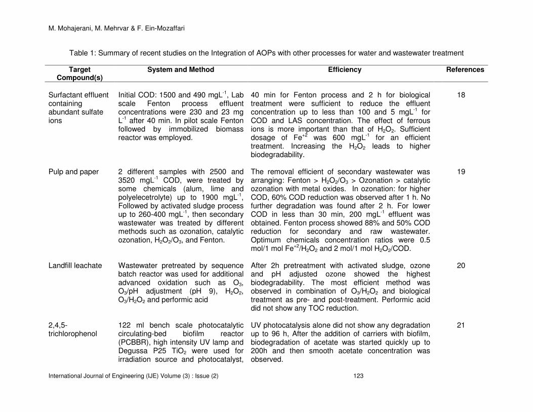
M. Mohajerani, M. Mehrvar & F. Ein-Mozaffari
International Journal of Engineering (IJE) Volume (3) : Issue (2) 123
Table 1: Summary of recent studies on the Integration of AOPs with other processes for water and wastewater treatment
Target Compound(s)
System and Method Efficiency References
Surfactant effluent containing abundant sulfate ions
Initial COD: 1500 and 490 mgL-1, Lab scale Fenton process effluent concentrations were 230 and 23 mg L-1 after 40 min. In pilot scale Fenton followed by immobilized biomass reactor was employed.
40 min for Fenton process and 2 h for biological treatment were sufficient to reduce the effluent concentration up to less than 100 and 5 mgL-1 for COD and LAS concentration. The effect of ferrous ions is more important than that of H2O2. Sufficient dosage of Fe+2 was 600 mgL-1 for an efficient treatment. Increasing the H2O2 leads to higher biodegradability.
18
Pulp and paper 2 different samples with 2500 and 3520 mgL-1 COD, were treated by some chemicals (alum, lime and polyelecetrolyte) up to 1900 mgL-1, Followed by activated sludge process up to 260-400 mgL-1, then secondary wastewater was treated by different methods such as ozonation, catalytic ozonation, H2O2/O3, and Fenton.
The removal efficient of secondary wastewater was arranging: Fenton > H2O2/O3 > Ozonation > catalytic ozonation with metal oxides. In ozonation: for higher COD, 60% COD reduction was observed after 1 h. No further degradation was found after 2 h. For lower COD in less than 30 min, 200 mgL-1 effluent was obtained. Fenton process showed 88% and 50% COD reduction for secondary and raw wastewater. Optimum chemicals concentration ratios were 0.5 mol/1 mol Fe+2/H2O2 and 2 mol/1 mol H2O2/COD.
19
Landfill leachate Wastewater pretreated by sequence batch reactor was used for additional advanced oxidation such as O3, O3/pH adjustment (pH 9), H2O2, O3/H2O2 and performic acid
After 2h pretreatment with activated sludge, ozone and pH adjusted ozone showed the highest biodegradability. The most efficient method was observed in combination of O3/H2O2 and biological treatment as pre- and post-treatment. Performic acid did not show any TOC reduction.
20
2,4,5-trichlorophenol
122 ml bench scale photocatalytic circulating-bed biofilm reactor (PCBBR), high intensity UV lamp and Degussa P25 TiO2 were used for irradiation source and photocatalyst,
UV photocatalysis alone did not show any degradation up to 96 h, After the addition of carriers with biofilm, biodegradation of acetate was started quickly up to 200h and then smooth acetate concentration was observed.
21

M. Mohajerani, M. Mehrvar & F. Ein-Mozaffari
International Journal of Engineering (IJE) Volume (3) : Issue (2) 124
respectively Hydroxyl-benzene
Photo-Fenton process in a 8 L 6-lamp CPC solar continuous photoreactor for treating raw river water and pretreated with slow sand filtration river water
Photolysis (with H2O2 and without Fe+3) showed 57% and 65% TOC reduction before and after SFF. Fe+3
concentration even as low as 1 mgL-1 depicted treatment improvement drastically. The presence of H2O2 under sunlight resulted in 50% mineralization.
22
Cibacron Red FN- R
A two stage aerobic-anaerobic method followed by photo-Fenton and ozonation processes was employed. The initial concentration of wastewater samples were 250, 1250, 3135 mgL-1.
Aerobic treatment showed less than 9% biodegradation after 28 days. The photo-Fenton process conducted with different ratios of Fe+3/H2O2, 10/250, 20/500, and 100/2500 mgl-1/mgl-1. DOC reduction was increased with increasing of Fe+3 and H2O2. After 30 min, DOC was reached a plateau and no further DOC removal was observed. Ozonation was carried out with different pH (3, 7, 10, and 10.5). pH 10.5 showed the best results (83% mineralization in 150 min). Neutral and acidic ozonation showed 48% degradation.
23
Phenol Hydrodynamic cavitation combined with advanced Fenton was employed for treating phenolic wastewater (2.5 mM).Hydrodynamic cavitation was generated by a liquid whistle reactor (LWR).
Results showed that both hydrodynamic cavitation and advanced Fenton have greater efficiency for lower phenol concentration. Continuous leaching resulted in higher concentration of iron ions with longer residence time. Increasing H2O2 dose in the range of 500-2000 mg/L led to greater TOC removal. In hydrodynamic cavitation, applied pressure had positive effect on TOC reduction. The closer distance between orifice and catalyst bed also performed better TOC removal.
24
Nonylphenol (NP) Sonochemical reactor equipped with 300kHz ultrasound transducer and cooling system, combined with biosoprtion of fungal cultures was used for treating different
US-Fenton process showed better degradation rate in case of lower initial contaminant concentration. Lowest initial concentration performed the complete mineralization. On the other hand, US only and Fenton only were ineffective after 1-2 h. Biosorption showed
25

M. Mohajerani, M. Mehrvar & F. Ein-Mozaffari
International Journal of Engineering (IJE) Volume (3) : Issue (2) 125
concentrations (100, 500, and 1000 ppm) of polluted water.
around 39 and 60% removal after 4 and 7 days. Initial concentration did not affect the removal percentage. In combined method 74 and 88% NP removal were observed after 1h US/Fenton and subsequent 4 and 7 days biosorption, respectively.
Methomyl, Dimethoate, Oxamyl, Cymoxanil, Pyrimethanil
50 mgL-1 concentration of each compound was used to be treated in combined AOP/biological method. AOPs were TiO2 photocatalysis and photo-Fenton. 35 L solar pilot plant equipped with 3 CPCs for TiO2 photocatalysis and 75 L solar pilot plant using 4 CPCs were employed for AOP stage. A 35 L aerobic immobilized biomass reactor (IBR) was used for biological treatment.
90% DOC removal was observed in 1197 and 512 min in case of case of TiO2 photocatalysis and photo-Fenton. Shorter irradiation time with two different iron concentrations (20 and 55 mgL-1) resulted in 50 and 72% DOC reduction. Photo-Fenton process showed greater pesticide degradation (more than twice) than the TiO2 photocatalysis. Pretreatment by photo-Fenton process decreased toxicity from 90 to 47%. Biodegradability tests showed 70% biodegradability is obtained after 12 days. Combined batch method showed 85% efficiency (23% AOP, 62% biological treatment). Combined batch AOP and continuous biological treatment showed more than 90% removal.
26
Procion blue A 130 ml plate and frame electrochemical flow cell and immobilized photocatalytic UV reactor were employed for degradation of 50 mg/L procion blue solution
Photo-electrochemical and photocatalytic electrochemical methods showed 98% dye degradation within 7 h. After 4 h different combined method showed more than 90% color removal. COD removal was proportional to applied current. The optimum TiO2 concentration was 40 mgL-1. Acidic condition performed greater degradation.
27-28
Reactive black 5 (RB5), Reactive blue 13 (RB13), Acid orange 7 (AO7)
Fenton processes followed by aerobic biological treatment (sequential batch reactors) were used for 50 mg/L dye solution. Different factors such as pH, H2O2 and Fe+2 were optimized.
pH 3 showed the highest decolorization for all dyes (more than 99%), Decolorization was increased at higher H2O2 concentration up to an optimal dose(50 mgL-1). optimal Fe+2 dose was found to be 15 mgL-1. 82, 89, and 84% COD removal was observed for RB5, RB13, and AO7, respectively.
29
Pharmaceutical The combination of solar AOP Industrial effluent containing α-methylphenylglycine 30
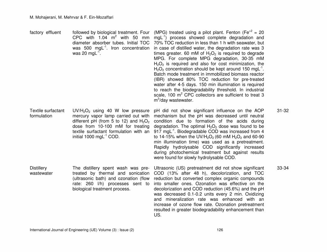
M. Mohajerani, M. Mehrvar & F. Ein-Mozaffari
International Journal of Engineering (IJE) Volume (3) : Issue (2) 126
factory effluent followed by biological treatment. Four CPC with 1.04 m2 with 50 mm diameter absorber tubes. Initial TOC was 500 mgL-1. Iron concentration was 20 mgL-1.
(MPG) treated using a pilot plant. Fenton (Fe+2 = 20 mgL-1) process showed complete degradation and 70% TOC reduction in less than 1 h with seawater, but in case of distilled water, the degradation rate was 3 times greater. 60 mM of H2O2 is required to degrade MPG. For complete MPG degradation, 30-35 mM H2O2 is required and also for cost minimization, the H2O2 concentration should be kept around 150 mgL-1. Batch mode treatment in immobilized biomass reactor (IBR) showed 80% TOC reduction for pre-treated water after 4-5 days. 150 min illumination is required to reach the biodegradability threshold. In industrial scale, 100 m2 CPC collectors are sufficient to treat 3 m3/day wastewater.
Textile surfactant formulation
UV/H2O2 using 40 W low pressure mercury vapor lamp carried out with different pH (from 5 to 12) and H2O2 dose from 10-100 mM for treating textile surfactant formulation with an initial 1000 mgL-1 COD.
pH did not show significant influence on the AOP mechanism but the pH was decreased until neutral condition due to formation of the acids during degradation. The optimal H2O2 dose was found to be 917 mgL-1. Biodegradable COD was increased from 4 to 14-15% when the UV/H2O2 (60 mM H2O2 and 60-90 min illumination time) was used as a pretreatment. Rapidly hydrolysable COD significantly increased during photochemical treatment but against results were found for slowly hydrolysable COD.
31-32
Distillery wastewater
The distillery spent wash was pre-treated by thermal and sonication (ultrasonic bath) and ozonation (flow rate: 260 l/h) processes sent to biological treatment process.
Ultrasonic (US) pretreatment did not show significant COD (13% after 48 h), decolorization, and TOC reduction but converted complex organic compounds into smaller ones. Ozonation was effective on the decolorization and COD reduction (45.6%) and the pH was decreased 0.1-0.2 units every 2 min. Oxidizing and mineralization rate was enhanced with an increase of ozone flow rate. Ozonation pretreatment resulted in greater biodegradability enhancement than US.
33-34
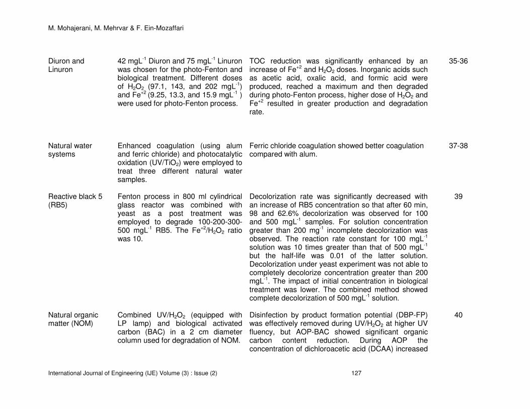
M. Mohajerani, M. Mehrvar & F. Ein-Mozaffari
International Journal of Engineering (IJE) Volume (3) : Issue (2) 127
Diuron and Linuron
42 mgL-1 Diuron and 75 mgL-1 Linuron was chosen for the photo-Fenton and biological treatment. Different doses of H2O2 (97.1, 143, and 202 mgL-1) and Fe+2 (9.25, 13.3, and 15.9 mgL-1 ) were used for photo-Fenton process.
TOC reduction was significantly enhanced by an increase of Fe+2 and H2O2 doses. Inorganic acids such as acetic acid, oxalic acid, and formic acid were produced, reached a maximum and then degraded during photo-Fenton process, higher dose of H2O2 and Fe+2 resulted in greater production and degradation rate.
35-36
Natural water systems
Enhanced coagulation (using alum and ferric chloride) and photocatalytic oxidation (UV/TiO2) were employed to treat three different natural water samples.
Ferric chloride coagulation showed better coagulation compared with alum.
37-38
Reactive black 5 (RB5)
Fenton process in 800 ml cylindrical glass reactor was combined with yeast as a post treatment was employed to degrade 100-200-300-500 mgL-1 RB5. The Fe+2/H2O2 ratio was 10.
Decolorization rate was significantly decreased with an increase of RB5 concentration so that after 60 min, 98 and 62.6% decolorization was observed for 100 and 500 mgL-1 samples. For solution concentration greater than 200 mg-1 incomplete decolorization was observed. The reaction rate constant for 100 mgL-1 solution was 10 times greater than that of 500 mgL-1
but the half-life was 0.01 of the latter solution. Decolorization under yeast experiment was not able to completely decolorize concentration greater than 200 mgL-1. The impact of initial concentration in biological treatment was lower. The combined method showed complete decolorization of 500 mgL-1 solution.
39
Natural organic matter (NOM)
Combined UV/H2O2 (equipped with LP lamp) and biological activated carbon (BAC) in a 2 cm diameter column used for degradation of NOM.
Disinfection by product formation potential (DBP-FP) was effectively removed during UV/H2O2 at higher UV fluency, but AOP-BAC showed significant organic carbon content reduction. During AOP the concentration of dichloroacetic acid (DCAA) increased
40
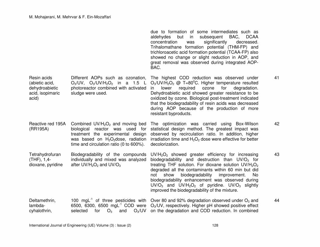
M. Mohajerani, M. Mehrvar & F. Ein-Mozaffari
International Journal of Engineering (IJE) Volume (3) : Issue (2) 128
due to formation of some intermediates such as aldehydes but in subsequent BAC, DCAA concentration was significantly decreased. Trihalomathane formation potential (THM-FP) and trichloroacetic acid formation potential (TCAA-FP) also showed no change or slight reduction in AOP, and great removal was observed during integrated AOP-BAC.
Resin acids (abietic acid, dehydroabietic acid, isopimaric acid)
Different AOPs such as ozonation, O3/UV, O3/UV/H2O2 in a 1.5 L photoreactor combined with activated sludge were used.
The highest COD reduction was observed under O3/UV/H2O2 @ T=800C. Higher temperature resulted in lower required ozone for degradation. Dehydroabietic acid showed greater resistance to be oxidized by ozone. Biological post-treatment indicated that the biodegradability of resin acids was decreased during AOP because of the production of more resistant byproducts.
41
Reactive red 195A (RR195A)
Combined UV/H2O2 and moving bed biological reactor was used for treatment the experimental design was based on H2O2dose, radiation time and circulation ratio (0 to 600%).
The optimization was carried using Box-Wilson statistical design method. The greatest impact was observed by recirculation ratio. In addition, higher irradiation time and H2O2 dose were effective for better decolorization.
42
Tetrahydrofuran (THF), 1,4-dioxane, pyridine
Biodegradability of the compounds individually and mixed was analyzed after UV/H2O2 and UV/O3
UV/H2O2 showed greater efficiency for increasing biodegradability and destruction than UV/O3 for treating THF solution. For dioxane solution UV/H2O2 degraded all the contaminants within 60 min but did not show biodegradability improvement. No biodegradability enhancement was observed during UV/O3 and UV/H2O2 of pyridine. UV/O3 slightly improved the biodegradability of the mixture.
43
Deltamethrin, lambda-cyhalothrin,
100 mgL-1 of three pesticides with 6500, 6300, 6500 mgL-1 COD were selected for O3 and O3/UV
Over 80 and 92% degradation observed under O3 and O3/UV, respectively. Higher pH showed positive effect on the degradation and COD reduction. In combined
44

M. Mohajerani, M. Mehrvar & F. Ein-Mozaffari
International Journal of Engineering (IJE) Volume (3) : Issue (2) 129
triadimenol degradation alone and combined with biological treatment.
process, O3/UV pre-treated solution showed higher degradation rate as compared to O3 pretreated, aerated, and raw solutions. Temperature was effective for enhancing the biodegradation.
Pulp and paper effluent
Combined AOP (photocatalysis or ozonation) and biological process was assisted for treating Kraft E1and black liquor effluent. TOC of these effluents were 934 and 128750 mgL-1.
Suspended photocatalysis showed a better decolorization for Kraft E1 with respect to ozonation (54 versus 27%). On the other hand, decolorization of black liquor effluent was more desirable with ozonation (14 versus 5%) due to the darkness of the solution. Photocatalysis showed 45% improvement for mineralization of Kraft E1, but ozonation enhanced 37% mineralization in combined method.
45
Green table olive processing wastewater
Lab scale and pilot scale of biological treatment followed by electrochemical reactor in the presence and absence of H2O2 was studied.
Inoculums’ size performed positive effect on COD removal so that 104 and 106 conidialml-1 showed 71.5 and 85.5% COD reduction. pH decreased faster for the high inoculum concentration. Most of the contaminants were degraded completely during biological treatment. Pre-treated solution was sent to electrolytic reactor with various H2O2dose (0, 2.5, and 5 v%). Results showed that the degradation was increased in the presence of H2O2. In pilot plant, 98% COD reduction was obtained during combined processes.
46
Dissolved organic matter (DOM) in drinking water
Single stage and multistage ozonation-biological and AOP-biological treatment were used for oxidizing DOC of the reservoir water and secondary effluent of the municipal wastewater when the DOC concentration was 20 mgL-1.
AOP-biological showed better mineralization rather than ozonation-biological. Further mineralization was achieved in multi-stage process, because in each biological stage, BDOC portion of the effluent was removed because this fraction can act as radical scavenger. Single stage and Multistage ozonation-biological did not perform significant oxidization for residence time greater than 15 min.
47
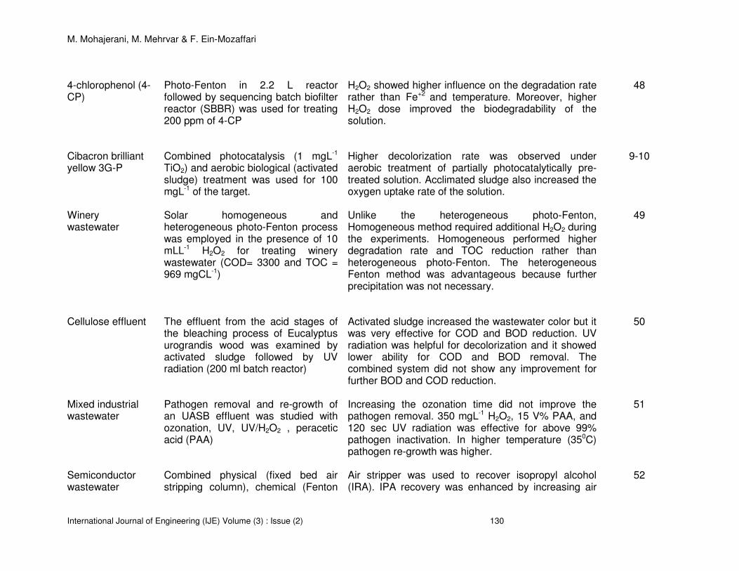
M. Mohajerani, M. Mehrvar & F. Ein-Mozaffari
International Journal of Engineering (IJE) Volume (3) : Issue (2) 130
4-chlorophenol (4-CP)
Photo-Fenton in 2.2 L reactor followed by sequencing batch biofilter reactor (SBBR) was used for treating 200 ppm of 4-CP
H2O2 showed higher influence on the degradation rate rather than Fe+2
and temperature. Moreover, higher H2O2 dose improved the biodegradability of the solution.
48
Cibacron brilliant yellow 3G-P
Combined photocatalysis (1 mgL-1 TiO2) and aerobic biological (activated sludge) treatment was used for 100 mgL-1 of the target.
Higher decolorization rate was observed under aerobic treatment of partially photocatalytically pre-treated solution. Acclimated sludge also increased the oxygen uptake rate of the solution.
9-10
Winery wastewater
Solar homogeneous and heterogeneous photo-Fenton process was employed in the presence of 10 mLL-1 H2O2 for treating winery wastewater (COD= 3300 and TOC = 969 mgCL-1)
Unlike the heterogeneous photo-Fenton, Homogeneous method required additional H2O2 during the experiments. Homogeneous performed higher degradation rate and TOC reduction rather than heterogeneous photo-Fenton. The heterogeneous Fenton method was advantageous because further precipitation was not necessary.
49
Cellulose effluent
The effluent from the acid stages of the bleaching process of Eucalyptus urograndis wood was examined by activated sludge followed by UV radiation (200 ml batch reactor)
Activated sludge increased the wastewater color but it was very effective for COD and BOD reduction. UV radiation was helpful for decolorization and it showed lower ability for COD and BOD removal. The combined system did not show any improvement for further BOD and COD reduction.
50
Mixed industrial wastewater
Pathogen removal and re-growth of an UASB effluent was studied with ozonation, UV, UV/H2O2 , peracetic acid (PAA)
Increasing the ozonation time did not improve the pathogen removal. 350 mgL-1 H2O2, 15 V% PAA, and 120 sec UV radiation was effective for above 99% pathogen inactivation. In higher temperature (350C) pathogen re-growth was higher.
51
Semiconductor wastewater
Combined physical (fixed bed air stripping column), chemical (Fenton
Air stripper was used to recover isopropyl alcohol (IRA). IPA recovery was enhanced by increasing air
52

M. Mohajerani, M. Mehrvar & F. Ein-Mozaffari
International Journal of Engineering (IJE) Volume (3) : Issue (2) 131
process), and biological (sequencing batch reactor (SBR)) was employed for treating a semiconductor wastewater and recover isopropyl alcohol.
flow rate, temperature and separation time. Fenton was very effective at pH between 2 and 5. Lower FeSO4 dose (lower than 5 mgL-1) showed greatest COD reduction. The removal rate was also increased under higher H2O2 flow rate up to 1 ml/min. Temperature was also beneficial for better Fenton efficiency. SBR with 12 cycles performed well to reduce COD from 600 to 100 mgL-1.
2,4-dichlorophenol (2,4-DCP)
100 ppm 2,4-DCP was treated in combined ozonation and biological treatment (activated sludge and acclimated biomass with phenol)
Ozonation improved the biodegradability of the solution from 0 to 0.25 and 0.48 for BOD5/COD and BOD21/COD. Activated sludge (non-acclimated with phenol) showed better removal rate than that of acclimated to phenol.
53
Linear alkylbenzene sulfonate (LAS)
76.6 L Pilot plant cylindrical photoreactor (UV/H2O2) for 12, 25, 50, 100 mgL-1 LAS
Biodegradability was increased during LAS photocatalysis especially for lower concentration of LAS. Over 90% of LAS was removed and biodegradability increased up to 0.4 during 90 min. Solution BOD was increased with photocatalysis residence time.
54
Methyl tert-butyl ether (MTBE)
3 L batch glass photoreactor equipped with 2 different UV lamps with wavelengths 365 and 254 nm employed for UV/H2O2 and UV/TiO2 followed by biodegradation using SBR
Over 90% MTBE removal achieved by UV/H2O2 within 1 h. Optimal H2O2 dose was 14 times greater than MTBE dose. UV-254 was more effective than UV-365 for both UV/H2O2 and UV/TiO2 in degrading MTBE. UV/H2O2 and UV/TiO2 were not effective for enhancing the biodegradability of solution.
55
Wool scouring effluent
Flocculation followed by aerobic biological treatment is being used to treat and UV/H2O2 was used as a post-treatment process. Biological treatment was also used as a post-treatment process.
BOD5 was increased during UV/H2O2 from <10 to 86 mgL-1. COD and TOC were removed by 75 and 85%, respectively. Decolorization was complete in less than 30 min. pH variation was ineffective on COD and TOC reduction. Higher COD removal was achieved in integrated AOP and Biological post-treatment.
56
M. Mohajerani, M. Mehrvar & F. Ein-Mozaffari
International Journal of Engineering (IJE) Volume (3) : Issue (2) 132
Oily wastewater from the lubricant unit
UV/H2O2 followed by biological (Pseudomonas putida DSM 437) treatment used to treat oily wastewater containing ethylene glycol, phenol, p-cresol, o-cresol. Direct biological results were compared to integrated system
Biodegradation alone showed 60% COD reduction. Fe+3/UV/H2O2 improved COD reduction rather than UV/H2O2 from 5 to 30% within 10 min. Integrated photolysis and biological showed greater organics removal relative to direct biodegradation. For example ethylene glycol was 100% removed from the solution. COD removal was increased from 60 to 72% by integrated process.
57
M. Mohajerani, M. Mehrvar & F. Ein-Mozaffari
International Journal of Engineering (IJE) Volume (3) : Issue (2) 133
3. PHYSICAL PROCESSES
Physical processes are widely used in the water and wastewater treatment plants. These physical techniques are based on the separation of one or more compounds from the waste stream. Because of the separation, the pollutant is transferred from one phase to another. Therefore, further treatment is required for the degradation of the contaminants in the second phase. Physical methods are employed mainly to separate large settleable and floating matter, clarify turbid solutions, recover and recycle valuable substances utilized in the main processes and separating inorganic materials. The conventional and advanced physical techniques include filtration, adsorption, gas stripping, and others. Physical treatment methods can be used before or after the advanced oxidation processes depending on the influent nature and its concentration as well as the AOPs operation conditions. Using physical techniques in wastewater treatment before and after the AOPs can be selected based on the consideration of various aspects of applications provided as follow: It is believed that the insoluble compounds and solid matter should be removed before any chemical or biochemical treatment because these materials may damage the equipment, increase the size of the equipment, results in a greater cost, and reduce the process efficiency.
For AOPs utilizing an irradiation source such as UV lamps (UV/H2O2, UV/O3, UV/TiO2, photo-Fenton and others), turbid solutions reduce the efficiency of the system. Turbidity decreases the local volumetric rate of energy absorption (LVREA) in the photoreactor, thus, the attenuation coefficient inside the reactor increases and it leads to smaller photochemically effective radiation field. Therefore, it is required to reduce the turbidity of the solutions by means of physical methods. The presence of some compounds in the solution that can adsorb on the surface of the catalyst results in deactivation of the catalyst due to the occupation of active sites. The lower amount of valent sites decreases the mass transfer between the catalyst and the species exist in the reactor, therefore, it reduces the number of hydroxyl radicals generated in the system. Some substances can also increase the agglomeration and aggregation of the catalyst powders in the system and reduce the mass transfer rate and system efficiency.
Free radical scavengers such as carbonate and bicarbonate ions reduce the number of hydroxyl radicals and system efficiency. Furthermore, these ions increase the attenuation coefficient and reduce the irradiation field. Physical and chemical methods can be employed for reducing such ions. Inorganic compounds such as heavy metals along with some chemicals may be detrimental to the AOPs and other subsequent processes. Therefore, they should be removed before AOPs. These substances are generally removed by adsorption, biosorption, and partition [58] methods such as granular activated carbon (GAC) column [59], biological activated carbon (BAC) column [60], unmodified clays (kaolinite and smectite) organoclays modified with short and long chain organic cations [61], or natural and modified zeolite [62].
It is beneficial to remove some compounds that have relatively lower oxidation potential than other compounds in the wastewater solutions by low cost physical methods. The separation of such compounds can help to keep the concentration of hydroxyl radicals high enough. The separation of volatile organic compounds is also helpful before ultrasonic AOPs. The oxidation of volatile organic compounds by acoustic cavitation is usually conducted by combustive reactions due to their extremely high temperature and pressure. If these compounds are removed before advanced oxidation processes, a lower power and ultrasonic intensity are required to oxidize the wastewater.
As mentioned earlier, AOPs change the characteristics and entity of the chemicals during the process, therefore, sometimes it is beneficial to use physical post-treatment. For example, the effluent of the AOPs may be adsorbed better by GAC. The most important issues in designing integrated processes such as fixed and operating costs should not be disregarded in order to achieve the desirable concentration limit of compounds.
4. BIOLOGICAL TREATMENT
Biological treatment methods are very common in wastewater treatment plants. These processes are useful for treating biodegradable waste streams. The use of biological treatment is attractive due to its low

M. Mohajerani, M. Mehrvar & F. Ein-Mozaffari
International Journal of Engineering (IJE) Volume (3) : Issue (2) 134
operating cost but the residence time is very high relative to that of other processes. On the other hand, the removal rate of advanced oxidation processes is relatively high while the operating cost is relatively expensive due to the use of reagents and irradiation sources. Capital and operating costs of biological treatment methods are 5-20 and 3-10 times cheaper than those of chemical methods, respectively [56-63]. Based on the cheaper construction and their operating cost, it is desirable to maximize the residence time and the removal rates of contaminants in biological processes. Biological treatment techniques are classified into two main groups: aerobic and anaerobic. Aerobic processes could be carried out by suspended (activated sludge), attached (biofilm reactor, trickling filter, and rotating disk contactor) or combined (moving bed biofilm reactor) depending on the operating conditions and wastewater characteristics. Wastewater can also be treated by anaerobic processes such as up-flow anaerobic sludge blanket (UASB), anaerobic fluidized bed reactor (AFBR), expanded granular sludge bed (EGSB), and anaerobic baffled reactor (ABR). Anaerobic techniques are usually employed for treating a concentrated municipal and industrial wastewater.
Depending on the type of wastewater, the nature of compounds and their concentrations, the integration of AOPs and biological processes could be designed in different configurations as follows: Wastewater solutions containing compounds which are toxic and inhibitory to biomass are necessary to be pre-treated by advanced oxidation processes. The AOPs reduce the toxicity of the wastewater. AOPs are also beneficial to pre-treat the wastewater containing bio-recalcitrant substances. This kind of wastewater is not biodegradable enough to be treated by biological processes. If the ratio of the BOD/COD of a wastewater is lower than 0.4, it is categorized as non-biodegradable or low in biodegradability [10,13]. Most AOPs enhance the biodegradability of the wastewater usually by decreasing the COD load. A class of waste solutions and wastewater streams is categorized as a biodegradable wastes with small amounts of recalcitrant compounds. This group contains a wide range of domestic and industrial effluents because none of the effluents after preliminary physical treatment is totally biodegradable. For this type of wastewater, AOPs could be applied as a pre-treatment or post-treatment stage depending on the concentrations of the compounds.
A wastewater with high COD or TOC is usually treated in an anaerobic process for decreasing the organic load of the effluent. AOPs are useful to be employed as a post-treatment of anaerobically treated effluent to further destroy the residual compounds dissolved in the wastewater. For a wastewater with a high organic loading that is not highly biodegradable, it is useful to apply integrated processes such as anaerobic process, AOP, and another aerobic process in sequence. In the first stage (anaerobic process), a large portion of COD is removed from the effluent. Then in AOP, non-biodegradable residuals are decomposed to smaller and more biodegradable molecules which are suitable for aerobic treatment in the final stage. The effluents with high biodegradable organic loading could be treated by integrated anaerobic-aerobic-AOP processes. The first two stages are employed to reduce the COD, BOD, and TOC and further polishing. Using the last stage is also effective for post-treatment of residuals. Multi-stage integrated AOP-biological treatment is also advantageous for a class of wastewater solutions (bio-recalcitrant and inhibitory streams) for decreasing operating cost of the treatment but it requires a relatively higher capital cost. Instead of using multi-stage integrated AOP-biological systems, recycling is another alternative for higher removal rate of contaminants. Recycling is helpful to keep the fixed cost lower than that of multi-stage processes. The circulation ratio is an important factor to determine the efficiency of the integrated AOP-biological method. The optimization of circulation ratio is beneficial to maximize the system efficiency and minimize the operating cost.
5. BIODEGRADABILITY
In the integration of advanced oxidation technologies and biological processes, the main responsibility of advanced oxidation processes is to enhance the biodegradability of the wastewater not the complete oxidation, mineralization, and COD or TOC reduction because COD and TOC can be reduced during low cost biological method. Therefore, it is desirable to increase the biodegradability of wastewater in the AOP stage as much as possible. The biodegradability of a solution can be evaluated as follows:
- BOD enhancement

M. Mohajerani, M. Mehrvar & F. Ein-Mozaffari
International Journal of Engineering (IJE) Volume (3) : Issue (2) 135
- BOD/COD enhancement
- BOD/TOC enhancement
Most of studies have emphasized on the enhancement of BOD/COD relative to the others. It is important to note that sometimes BOD/COD enhancement is due to only COD reduction and it may not result in a higher biodegradability. Although the COD of the solution is decreased, AOP may decompose the complex and toxic compounds and produce a relatively more toxic daughter compounds with lower BOD than that of the parent compounds. Therefore, the biodegradability is increased in the case of both COD or TOC reduction and BOD enhancement.
6. INTEGRATION OR COMBINATION?
In recent years, different studies have tried to increase the efficiency of AOPs by using various methods such as integrated (sequential) and combined (simultaneous) processes. As explained earlier, the main purpose of integrating different treatment methods is to enhance the process efficiency as well as to reduce the operating cost. On the other hand, a combined process is used for intensification of the process. Neelavannan et al. (2007) [27-28] showed that combined photocatalytic and electrochemical processes performed a better procion blue dye degradation rate as compared to that of integrated processes. The main parameter in combined processes to evaluate the effectiveness of the system is the synergetic effect. Synergetic effect is a parameter that shows the enhancement of organic compounds’ degradation under combined method relative to the linear combination (sequential) method. The synergetic effect could be estimated as follow [17]:
constant rate methods individual ofsummation Linear
constant ratereaction Combinedeffect Synergetic = (1)
The existence of two or more advanced oxidation processes often results in a greater degradation rate due to several factors that are explained in details in the next sections. The design, construction, operation, and maintenance of combined (simultaneous) advanced oxidation processes is more difficult than those of the individual methods, but by combining various technologies, lower capital and operating costs are achievable. It is obvious that the purpose of combination of advanced oxidation processes is to enhance the degradation rate that is not achievable by a single process alone under the same condition. Several factors are required to be considered simultaneously in combined advanced oxidation technologies. These factors are as follows:
Method: The strength of different combined methods is useful to decide whether this hybrid system is beneficial. For those methods employed to degrade organic compounds or to enhance the biodegradability, the combined method which has the greatest removal rate would be the best choice. On the other hand, if the goal of the treatment is mineralization, it is better to select the combined system that has the highest TOC reduction rate.
Residence time: The product of the synergetic effect and residence time is equal to the summation of individual processes’ residence times.
Cost: Fixed and operating costs of hybrid methods are less than those of the summation of different individual process. By increasing the synergetic effect, these costs can be even less. Synergetic effects of less than one are almost always not practical due to the lower degradation rate and higher maintenance cost. It is also not economical to combine different methods with the synergetic effect slightly greater than one when the contribution of a method is lower in the degradation of organic compounds and synergetic effect.
Energy: In combining different single processes, the amount of energy or power required for the degradation should be considered. Methods employing UV, ultrasonic irradiation, ozone generation, gas sparging, and mechanical mixing consume a higher amount of energy relative to others, but they enhance the degradation rate.

M. Mohajerani, M. Mehrvar & F. Ein-Mozaffari
International Journal of Engineering (IJE) Volume (3) : Issue (2) 136
There are many studies in combining different AOPs such as combined photocatalysis and ultrasound [64-71], ozonation and ultrasound [72-74], photo-Fenton processes [75-77], and combined Fenton, photo-Fenton, and ultrasound [78-85]. Combining an advanced oxidation technology and biological process is very rare because hydroxyl radicals’ formation during the AOPs may be inhibitory to biomass. Moreover, the presence of H2O2 is also poisonous to microorganisms. Therefore, it is better to use the combined system in the AOP part to enhancing the oxidation and biodegradability in less time. In studying the behavior of the integration of combined AOPs and biological treatment processes, it is better to define a new parameter to depict the biodegradability enhancement due to the combination of different methods.
processes individualby t enhancemenbility biodegrada Total
process combinedby t enhancemenbility Biodegrada t enhancemenbility biodegrada Synergetic = (2)
This equation shows the amount of additional BOD produced by combined process. This equation is useful in evaluating the integrated AOP-biological process efficiency as the biodegradability enhancement is necessary to be achieved.
7. KINETICS AND MODELING OF INTEGRATED PROCESSES
AOPs have their own kinetics and mechanisms for oxidizing organic compounds depending on irradiation source characteristics and the type and the dose of reagents functioning in the reactor. Different studies carried out for modeling AOPs such as UV/H2O2 [5, 86], photocatalysis [87], and Fenton [88-89]. A few studies were carried out for modeling of integration processes [86, 90-91].
7.1 BIOLOGICAL MODELING
Usually biological reactions are modeled by Monod [90, 92-95], Haldane [90], two-step Haldane [90], Contois [96-97], and Grau [98]. The Monod equation has been found as an acceptable and powerful mathematical expression fitted to experimental data described as follows [90]:
CODK
COD
COD += maxµµ (3)
where µ and µmax are the specific and maximum specific growth rates of microorganisms, KCOD is the half saturation constant, and COD is standing for any limiting organic source (COD concentration), respectively. In case of KCOD << COD that is applicable to no inhibition, Monod equation can be simplified as follows [90, 94]:
( )
maxmax
1µµµ ≅
+==
CODK
COD
dt
VSSd
Vss COD
(4)
Cell yield coefficient can be defined based on the COD consumption and volatile suspended solids (VSS) production during aerobic biochemical degradation and it can be defined as follows [90]:
CODCOD
VSSVSSY CODVSS
−
−=
0
0/ (5)
where VSSo and VSS are the initial and final volatile suspended solids in the bioreactor, and CODo– COD is the organic consumption during the biological treatment. Rivas et al., (2003) [91] also employed Equation (5) based on the utilization of biodegradable COD fraction.
Monod expression can be employed for modeling as follows:
[ ][ ] [ ]
[ ][ ] [ ][ ] [ ]
−
−
+==−
0
0max
/
.1
VSSVSS
CODCOD
CODK
COD
Ydt
CODd
VSS CODCODVSS
µµ (6)

M. Mohajerani, M. Mehrvar & F. Ein-Mozaffari
International Journal of Engineering (IJE) Volume (3) : Issue (2) 137
[ ] [ ][ ][ ] [ ]
[ ][ ][ ] [ ]( )0
max
0
0max
)( VSSVSSK
CODVSS
VSSVSSK
CODVSS
dt
CODd
CODCOD −−
−=−
µµ (7)
If A = [ ][ ][ ] [ ] )( 0
0max
VSSVSSK
CODVSS
COD −
µ , B =
[ ][ ] [ ]( )0
max
VSSVSSK
VSS
COD −
µ, and KCOD << [COD], after integration of the
equation, following equation can be achieved:
[ ][ ]
BtCODBA
CODBA=
+
+
0
ln (8)
A plot of the left hand side of Equation (8) versus t should give a straight line to find the parameters of interest.
7.2 MODELING OF ADVANCED OXIDATION TECHNOLOGIES
Modeling of the AOPs is carried out based on the summation of degradation rates in different methods such as direct photolysis, direct ultrasonolysis, direct ozonolysis, the degradation due to hydroxyl radicals attack, and the degradation due to the synergetic effect. A typical kinetics of US/UV/H2O2 and US/UV reaction can be written based on the degradation rate of individual processes and the impact of the synergetic effect as follows [73, 83, 86]:
[ ] [ ] [ ]isynergy
CL
i
ii
C
CiOHipyri CKe
CICKCK
dt
dCi
iii −
−
++=−∑−
∑
ε
ε
εφ
303.2
0 1.... (9)
where , , , and are quantum yield, light intensity, molar absorptivity, and the compounds’ concentration. Kpyr and K.OH are the constant of pyrolytic decomposition rate of organic compounds and the constant of the rate of reaction between organics and hydroxyl radicals, respectively. is the
synergetic effect constant representing the degradation rate enhancement due to combined treatment methods. In the combined UV/US/H2O2 processes, organic compounds are oxidized through direct photolysis, combustion or pyrolysis, free radical attack, and the synergetic effect predicted by combined system. If the completely mixed solution is assumed, the degradation of contaminants is due to the location of UV lamps, ultrasonic transducer, and the physical and geometrical characteristics of the reactor. The location of the ultraviolet lamps and ultrasonic irradiation is also very critical for determining the synergetic effect. The highest synergetic effect is predicted when the UV lamps bounded with ultrasonic irradiation field. In other words, maximum local volumetric rate of energy absorption (LVREA) and ultrasonic field overlap can produce a highest synergetic effect. Therefore, for designing an AOP system, the location of internal equipment employing for irradiation should be carefully selected to maximize the synergetic effect of the process.
The experiments for the advanced oxidation processes are usually conducted by optimizing the operating conditions and photoreactor characteristics since the efficiency of the AOPs is affected by various variables such as the concentration of initial compounds, residence time, H2O2 dose, photocatalyst concentration, temperature, and pH. Therefore, it is necessary to employ the optimal condition. Recently, the experiments are conducted to analyze the effects of different parameters on the process effectiveness. Experimental design is also useful in order to avoid one-factor-at-a-time approach, where one variable was changed while keeping the others constant. Experimental design also helps to find the complex interaction between independent variables. Among these interactions, synergetic effect leads to the generation of higher hydroxyl radicals and it requires to be carefully optimized.
8. OPTIMIZATION OF THE INTEGRATED PROCESSES

M. Mohajerani, M. Mehrvar & F. Ein-Mozaffari
International Journal of Engineering (IJE) Volume (3) : Issue (2) 138
Integrated processes are optimized to enhance the mineralization efficiency. Process optimization can be based on the residence time, the energy consumption, and the total cost. The optimization of each parameter depends on the environmental regulation, the process location, and characteristics of individual processes.
8.1 Residence time
The minimization of the total residence time of all processes involved in integrated system is the objective function of the optimization. The constraints are also the limits of residence times of individual processes including the mass balance of each component in every process. Therefore, the objective function of integrated processes based on the total residence time is as follows [12]:
Minimize: BCPF θθθ ++= (10)
where Pθ , Cθ , and Bθ (h) are physical, chemical, and biological residence times, respectively. F (h) is
the total residence time of the system. The constraints are usually defined such that θp and θb should be positive where Cθ should be greater than a value so that a reasonable biodegradability is achieved.
8.2 Fixed cost
The fixed or capital cost of AOPs is relatively higher as compared to other treatment methods. Hirvonen et al. (1998) [99] provided the capital and operating cost of UV/H2O2 (AOPs) and activated carbon. Estimated fixed costs of different treatment methods based on the depreciation period (40 years) are provided as follow [99]:
Photoreactors:
( )
×
××
×+=
L
m
VFC
C
C
C1000
1
3652440
500,140000,85 3
θ
(11)
where FCC ($/L) is a typical UV/H2O2 fixed cost, and VC (m3) is the volume of the photoreactor. (h) is the residence time of the wastewater in the photoreactor. The fixed cost for a UV/H2O2 process is usually $58,000 plus the cost of UV lamp which is $15,000 per year. The maximum allowable useful life estimate under U.S.A. income tax regulations is 40 years which can be considered as depreciation time.
Activated carbon:
( )
×
××
=L
m
VFC
P
P
P1000
1
3652440
000,58 3
θ
(12)
where FCp ($/L) represents the fixed cost of a typical activated carbon column and Vp (m3) is the volume
of the column. $58,000 is the capital cost for a typical activated carbon column.
Biological reactor:
( )
( )
××
+
×××
=
B
B
B
B
BV
V
FC
θ
θ
3652440
403,368365244072
(13)
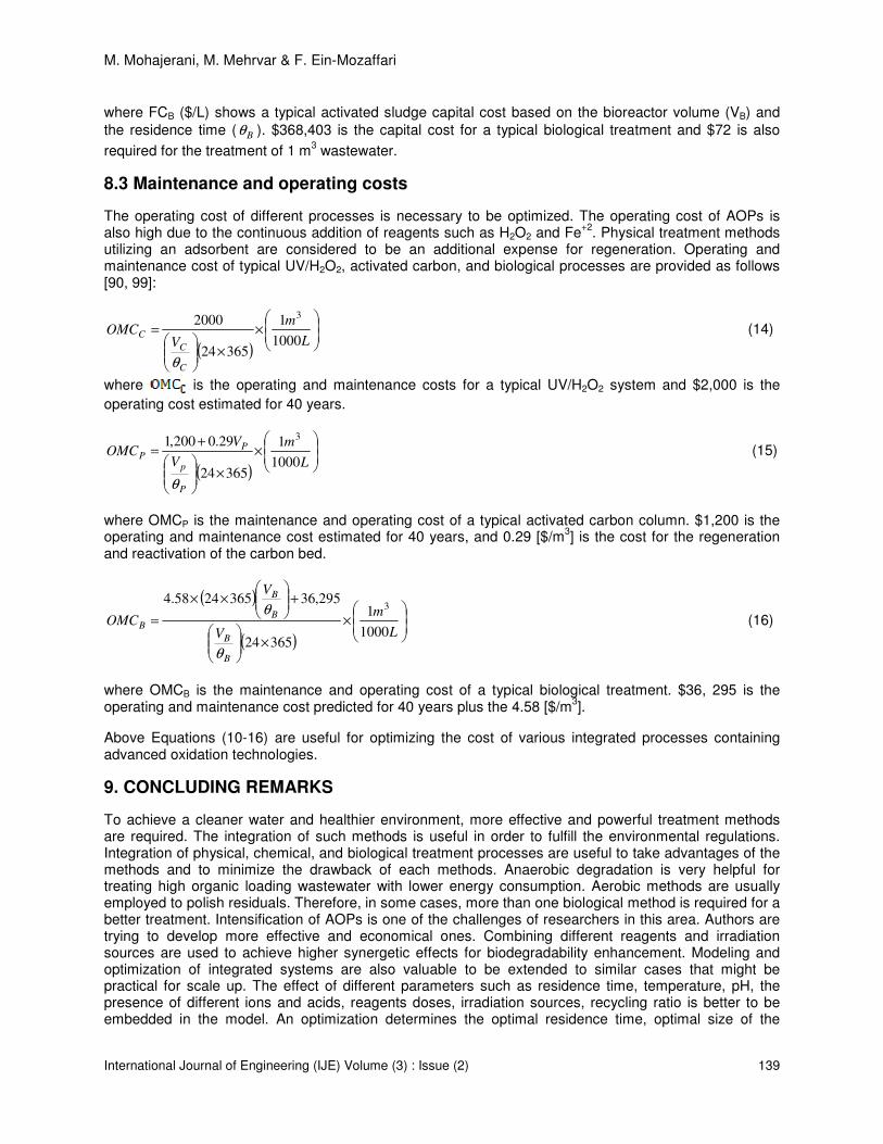
M. Mohajerani, M. Mehrvar & F. Ein-Mozaffari
International Journal of Engineering (IJE) Volume (3) : Issue (2) 139
where FCB ($/L) shows a typical activated sludge capital cost based on the bioreactor volume (VB) and the residence time ( Bθ ). $368,403 is the capital cost for a typical biological treatment and $72 is also
required for the treatment of 1 m3 wastewater.
8.3 Maintenance and operating costs
The operating cost of different processes is necessary to be optimized. The operating cost of AOPs is also high due to the continuous addition of reagents such as H2O2 and Fe+2. Physical treatment methods utilizing an adsorbent are considered to be an additional expense for regeneration. Operating and maintenance cost of typical UV/H2O2, activated carbon, and biological processes are provided as follows [90, 99]:
( )
×
×
=
L
m
VOMC
C
C
C1000
1
36524
2000 3
θ
(14)
where is the operating and maintenance costs for a typical UV/H2O2 system and $2,000 is the operating cost estimated for 40 years.
( )
×
×
+=
L
m
V
VOMC
P
p
PP
1000
1
36524
29.0200,1 3
θ
(15)
where OMCP is the maintenance and operating cost of a typical activated carbon column. $1,200 is the operating and maintenance cost estimated for 40 years, and 0.29 [$/m3] is the cost for the regeneration and reactivation of the carbon bed.
( )
( )
×
×
+
××
=L
m
V
V
OMC
B
B
B
B
B1000
1
36524
295,363652458.43
θ
θ (16)
where OMCB is the maintenance and operating cost of a typical biological treatment. $36, 295 is the operating and maintenance cost predicted for 40 years plus the 4.58 [$/m3].
Above Equations (10-16) are useful for optimizing the cost of various integrated processes containing advanced oxidation technologies.
9. CONCLUDING REMARKS
To achieve a cleaner water and healthier environment, more effective and powerful treatment methods are required. The integration of such methods is useful in order to fulfill the environmental regulations. Integration of physical, chemical, and biological treatment processes are useful to take advantages of the methods and to minimize the drawback of each methods. Anaerobic degradation is very helpful for treating high organic loading wastewater with lower energy consumption. Aerobic methods are usually employed to polish residuals. Therefore, in some cases, more than one biological method is required for a better treatment. Intensification of AOPs is one of the challenges of researchers in this area. Authors are trying to develop more effective and economical ones. Combining different reagents and irradiation sources are used to achieve higher synergetic effects for biodegradability enhancement. Modeling and optimization of integrated systems are also valuable to be extended to similar cases that might be practical for scale up. The effect of different parameters such as residence time, temperature, pH, the presence of different ions and acids, reagents doses, irradiation sources, recycling ratio is better to be embedded in the model. An optimization determines the optimal residence time, optimal size of the

M. Mohajerani, M. Mehrvar & F. Ein-Mozaffari
International Journal of Engineering (IJE) Volume (3) : Issue (2) 140
equipment, optimal reagents doses, optimal operating condition such as oxygen concentration in the bioreactor, and optimal biodegradability achieved after advanced oxidation process.
ACKNOWLEDGEMENT
The financial support of Natural Sciences and Engineering Research Council of Canada (NSERC) and Ryerson University is greatly appreciated.
REFERENCES
1. P.R. Gogate and A.B. Pandit. “A review of imperative technologies for wastewater treatment II: Hybrid methods”. Advances in Environmental Research, 8 (3-4): 553-597, 2004
2. P.R. Gogate and A.B. Pandit. “A review of imperative technologies for wastewater treatment I: Oxidation technologies at ambient conditions”. Advances in Environmental Research, 8 (3-4): 501-551, 2004
3. P. Paraskeva and E. Diamadopoulos. “Technologies for olive mill wastewater (OMW) treatment: A review”. J. Chem. Technol. Biot., 81 (9):1475-1485, 2006
4. S. Esplugas, D.M. Bila, L.G.T. Krause, and M. Dezotti “Ozonation and advanced oxidation technologies to remove endocrine disrupting chemicals (EDCs) and pharmaceuticals and personal care products (PPCPs) in water effluents”. J. Hazard. Mater., 149 (3): 631-642, 2007
5. M.B. Johnson and M. Mehrvar. “Aqueous metronidazole degradation by UV/H2O2 process in single- and multi-lamp tubular photoreactors: Kinetics and reactor design”. Ind. Eng. Chem. Res., 47 (17): 6525-6537, 2008
6. H.K. Moo-Young. “Pulp and paper effluent management”. Water Environ. Res., 79 (10): 1733-1741, 2007
7. G. Crini. “Non-conventional low-cost adsorbents for dye removal: A review”. Bioresour. Technol., 97 (9): 1061-1085, 2006
8. P.C. Vandevivere, R. Bianchi and W. Verstraete. “Treatment and reuse of wastewater from the textile wet-processing industry: Review of emerging technologies”. J. Chem. Technol. Biot., 72 (4): 289-302, 1998
9. T. Aye, W.A. Anderson, and M. Mehrvar. “Photocatalytic treatment of cibacron brilliant yellow 3G-P (reactive yellow 2 textile dye)”. J. Environ. Sci. Heal. A, 38 (9): 1903-1914, 2003
10. T. Aye, M. Mehrvar, and W.A. Anderson. “Effects of photocatalysis on the biodegradability of Cibacron Brilliant Yellow 3G-P (Reactive Yellow 2)”. J. Environ. Sci. Heal. A, 39 (1): 113-126, 2004
11. S. Renou, J.G. Givaudan, S. Poulain, F. Dirassouyan, and P. Moulin. “Landfill leachate treatment: Review and opportunity”. J. Hazard. Mater., 150 (3): 468-493, 2008
12. J.P. Scott and D.F. Ollis. “Integration of chemical and biological oxidation processes for water treatment: review and recommendations”. Environ. Prog., 14 (2): 88-103, 1995
13. G.B. Tabrizi and M. Mehrvar. “Integration of advanced oxidation technologies and biological processes: Recent developments, trends, and advances”. J. Environ. Sci. Heal. A, 39 (11-12): 3029-3081, 2004
14. D. Mantzavinos and E. Psillakis. “Enhancement of biodegradability of industrial wastewaters by chemical oxidation pre-treatment”. J. Chem. Technol. Biot., 79 (5): 431-454, 2004

M. Mohajerani, M. Mehrvar & F. Ein-Mozaffari
International Journal of Engineering (IJE) Volume (3) : Issue (2) 141
15. O. Legrini, E. Oliveros, and A.M. Braun. “Photochemical processes for water treatment”. Chem. Rev., 93 (2): 671-698, 1993
16. B.R. Ball, K.V. Brix, M.S. Brancato, M.P. Allison and S.M. Vail. “Whole effluent toxicity reduction by ozone”, Environ. Prog., 16 (2): 121–124, 1997
17. J.-W. Kang and M. R. Hoffmann. “Kinetics and mechanism of the sonolytic destruction of methyl tert-butyl ether by ultrasonic irradiation in the presence of ozone”. Environ. Sci. Technol., 32 (20): 3194-3199, 1998
18. X.-J. Wang, Y. Song, and J.-S. Mai, “Combined Fenton oxidation and aerobic biological processes for treating a surfactant wastewater containing abundant sulfate”. J. Hazard. Mater., 160 (2-3): 344-348, 2008
19. O. Tünay, E. Erdeml, I. Kabdaşli, and T. Ölmez, “Advanced treatment by chemical oxidation of pulp and paper effluent from a plant manufacturing hardboard from waste paper”. Environ. Technol., 29 (10): 1045-1051, 2008
20. M. Hagman, E. Heander and J.L.C. Jansen. “Advanced oxidation of refractory organics in leachate- potential methods and evaluation of biodegradability of the remaining substrate”. Environ. Technol., 29 (9): 941-946, 2008
21. M.D. Marsolek, C.I. Torres, M. Hausner, and B.E. Rittmann. “Intimate coupling of photocatalysis and biodegradation in a photocatalytic circulating-bed biofilm reactor”. Biotechnol. Bioeng., 101 (1): 83-92, 2008
22. A. Moncayo-Lasso, C. Pulgarin, and N. Benítez. “Degradation of DBPs’ precursors in river water before and after slow sand filtration by photo-Fenton process at pH 5 in a solar CPC reactor”. Water Res., 42 (15): 4125-4132, 2008
23. J. García-Montaño, X. Domènesh, J.A. García-Hortal, F. Torrades, and J. Peral. “The testing of several biological and chemical coupled treatments for Cibacron Red FN-R azo dye removal”. J. Hazard. Mater., 154 (1-3): 484-490, 2008
24. A.G. Chakinala, D.H. Bremner, P.R. Gogate, K.-C. Namkung, and A.E. Burgess, “Multivariate analysis of phenol mineralisation by combined hydrodynamic cavitation and heterogeneous advanced Fenton processing”. Appl. Catal. B-Environ., 78 (1-2): 11-18, 2008
25. G. Cravotto, S. Di Carlo, A. Binello, S. Mantegna, M. Girlanda, and A. Lazzari. “Integrated sonochemical and microbial treatment for decontamination of nonylphenol-polluted water”. Water Air Soil Poll., 187 (1-4): 353-359, 2008
26. I. Oller, , S. Malato, J.A Sánchez-Pérez, M.I. Maldonado, and R. Gassó, “Detoxification of wastewater containing five common pesticides by solar AOPs-biological coupled system”. Catal. Today, 129 (1-2 SPEC. ISS.): 69-78, 2007
27. M.G. Neelavannan, M. Revathi, and C. Ahmed Basha. “Photocatalytic and electrochemical combined treatment of textile wash water”. J. Hazard. Mater., 149 (2): 371-378, 2007
28. M.G. Neelavannan and C. Ahmed Basha. “Electrochemical-assisted photocatalytic degradation of textile washwater”. Sep. Purif. Technol., 61 (2): 168-174, 2008
29. B. Lodha and S. Chaudhari. “Optimization of Fenton-biological treatment scheme for the treatment of aqueous dye solutions”. J. Hazard. Mater., 148 (1-2): 459-466, 2007
30. S. Malato, J. Blanco, M.I. Maldonado, I. Oller, W. Gernjak, and L. Pérez-Estrada. “Coupling solar photo-Fenton and biotreatment at industrial scale: Main results of a demonstration plant”. J. Hazard. Mater., 146 (3): 440-446, 2007

M. Mohajerani, M. Mehrvar & F. Ein-Mozaffari
International Journal of Engineering (IJE) Volume (3) : Issue (2) 142
31. I. Arslan-Alaton and S. Dogruel. “Pre-treatment of penicillin formulation effluent by advanced oxidation processes”. J. Hazard. Mater., 112 (1-2): 105-113, 2004
32. I. Arslan-Alaton, S. Dogruel, E. Baykal, and G. Gerone. “Combined chemical and biological oxidation of penicillin formulation effluent”. J. Environ. Manage., 73 (2): 155-163, 2004
33. P.C. Sangave, P.R. Gogate, and A.B. Pandit, “Combination of ozonation with conventional aerobic oxidation for distillery wastewater treatment”. Chemosphere, 68 (1): 32-41, 2007
34. P.C. Sangave, P.R. Gogate, and A.B. Pandit. “Ultrasound and ozone assisted biological degradation of thermally pretreated and anaerobically pretreated distillery wastewater”. Chemosphere, 68 (1): 42-50, 2007
35. M. José-Farré, J. García-Montaño, N. Ruiz, , I. Muñoz, X. Domènech, and J. Peral. “Life cycle assessment of the removal of Diuron and Linuron herbicides from water using three environmentally friendly technologies”. Environ. Technol., 28 (7): 819-830, 2007
36. M. José-Farré, S. Brosillon, X. Domènech, and J. Peral. “Evaluation of the intermediates generated during the degradation of Diuron and Linuron herbicides by the photo-Fenton reaction”. J. Photoch. Photobio. A., 189 (2-3): 364-373, 2007
37. C.S. Uyguner, S.A. Suphandag, A. Kerc, and M. Bekbolet. “Evaluation of adsorption and coagulation characteristics of humic acids preceded by alternative advanced oxidation techniques”. Desalination, 210 (1-3): 183-193, 2007
38. C.S. Uyguner, M. Bekbolet, and H. Selcuk “A comparative approach to the application of a physico-chemical and advanced oxidation combined system to natural water samples”. Sep. Sci. Technol., 42 (7): 1405-1419, 2007
39. M.S. Lucas, A.A. Dias, A. Sampaio, C. Amaral, and J. Peres. “Degradation of a textile reactive azo dye by a combined chemical-biological process: Fenton’s reagent-yeast”. Water Res., 41 (5): 1103-1109, 2007
40. R. Toor, and M. Mohseni, “UV-H2O2 based AOP and its integration with biological activated carbon treatment for DBP reduction in drinking water”. Chemosphere, 66 (11): 2087-2095, 2007
41. S. Ledakowicz, M. Michniewicz, A. Jagiella, J. Stufka-Olczyk, and M. Martynelis, “Elimination of resin acids by advanced oxidation processes and their impact on subsequent biodegradation”. Water. Res., 40 (18): 3439-3446, 2006
42. G. Sudarjanto, B. Keller-Lehmann, and J. Keller. “Optimization of integrated chemical-biological degradation of a reactive azo dye using response surface methodology”. J. Hazard. Mater., 138 (1): 160-168, 2006
43. H.L. Quen and C.B. Raj. “Evaluation of UV/O3 and UV/H2O2 processes for nonbiodegradable compounds: Implications for integration with biological processes for effluent treatment”. Chem. Eng. Commun., 193 (10): 1263-1276, 2006
44. W.K. Lafi and Z. Al-Qodah. “Combined advanced oxidation and biological treatment processes for the removal of pesticides from aqueous solutions”. J. Hazard. Mater., 137 (1): 489-497, 2006
45. S.G. Moraes, N. Durán, and R.S. Freire. “Remediation of Kraft E1 and black liquor effluents by biological and chemical processes”. Environ. Chem. Lett., 4 (2): 87-91, 2006
46. A. Kyriacou, K.E. Lasaridi, M. Kotsou, C. Balis, and G. Pilidis. “Combined bioremediation and advanced oxidation of green table olive processing wastewater”. Process Biochem., 40 (3-4): 1401-1408, 2005

M. Mohajerani, M. Mehrvar & F. Ein-Mozaffari
International Journal of Engineering (IJE) Volume (3) : Issue (2) 143
47. Fahmi, W. Nishijima, and M. Okada. “Improvement of DOC removal by multi-stage AOP-biological treatment”. Chemosphere, 50 (8): 1043-1048, 2003
48. J. Bacardit, V. García-Molina, B. Bayarri, J. Giménez, E. Chamarro, C. Sans, and S. Esplugas. “Coupled photochemical-biological system to treat biorecalcitrant wastewater”. Water Sci. Technol., 55 (12): 95-100, 2007
49. R. Mosteo, M.P. Ormad, and J.L. Ovelleiro. “Photo-Fenton processes assisted by solar light used as preliminary step to biological treatment applied to winery wastewaters”. Water Sci. Technol., 56 (2): 89-94, 2007
50. F.T. Silva, L.R. Mattos, and T.C.B. Paiva. “Treatment of an ECF effluent by combined use of activated sludge and advanced oxidation process”. Water Sci. Technol., 55 (6): 151-156, 2007
51. A. Yasar, N. Ahmad, H. Latif, and A.A.A. Khan. “Pathogen re-growth in UASB effluent disinfected by UV, O3, H2O2, and advanced oxidation processes”. Ozone-Sci. Eng., 29 (6): 485-492, 2007
52. S.H. Lin and C.D. Kiang. “Combined physical, chemical and biological treatments of wastewater containing organics from a semiconductor plant”. J. Hazard. Mater., 97 (1-3): 159-171, 2003
53. S. Contreras, M. Rodríguez, F. Al Momani, C. Sans, and S. Esplugas. “Contribution of the ozonation pre-treatment to the biodegradation of aqueous solutions of 2,4-dichlorophenol”. Water Res., 37 (13): 3164-3171, 2003
54. M. Mehrvar, G.B. Tabrizi, and N. Abdel-Jabbar. “Effects of pilot-plant photochemical pre-treatment (UV/H2O2) on the biodegradability of aqueous linear alkylbenzene sulfonate (LAS)”. Int. J. Photoenergy., 7 (4): 169-174, 2005
55. A. Asadi and M. Mehrvar. “Degradation of aqueous methyl tert-butyl ether by photochemical, biological, and their combined processes”. Int. J. Photoenergy., art. No. 19790, 2006
56. Poole, A.J. “Treatment of biorefractory organic compounds in wool scour effluent by hydroxyl radical oxidation”. Water. Res., 38 (14-15): 3458-3464, 2004
57. D. Mamma, S. Gerontas, C.J. Philippopoulos, P. Christakopoulos, B.J. Macris, and D. Kekos. “Combined photo-assisted and biological treatment of industrial oily wastewater”. J. Environ. Sci. Heal. A, 39 (3): 729-740, 2004
58., D. Mohan and Jr., C.U. Pittman. “Arsenic removal from water/wastewater using adsorbents- A critical review”. J. Hazard. Mater., 142 (1-2): 1-53, 2007
59. G.M. Walker and L.R. Weatherley. “Adsorption of acid dyes on to granular activated carbon in fixed beds”. Water Res., 31 (8): 2093-2101, 1997
60. C.Y. Yin, M.K. Aroua, and W.M.A.W. Daud. “Review of modifications of activated carbon for enhancing contaminant uptakes from aqueous solutions”. Sep. Purif. Technol., 52 (3): 403-415, 2007
61. Z. Bouberka, S. Kacha, M. Kameche, S. Elmaleh, and Z. Derriche. “Sorption study of an acid dye from an aqueous solutions using modified clays”. J. Hazard. Mater., 119 (1-3): 117-124, 2005
62. U. Wingenfelder, B. Nowack, G. Furrer, and R. Schulin. “Adsorption of Pb and Cd by amine-modified zeolite”. Water Res., 39 (14): 3287-3297, 2005
63. A. Marco, S. Esplugas, and G. Saum. “How and why combine chemical and biological processes for wastewater treatment”. Water Sci. Technol., 35 (4): 321-327, 1997
64. L. Davydov, E.P. Reddy, P. France, and P.G. Smirniotis. “Sonophotocatalytic destruction of organic contaminants in aqueous systems on TiO2 powders”. Appl. Catal. B-Environ., 32 (1-2): 95-105, 2001

M. Mohajerani, M. Mehrvar & F. Ein-Mozaffari
International Journal of Engineering (IJE) Volume (3) : Issue (2) 144
65. V. Ragaini, E. Selli, C. Letizia Bianchi, and C. Pirola. “Sono-photocatalytic degradation of 2-chlorophenol in water: Kinetic and energetic comparison with other techniques”. Ultrason. Sonochem., 8 (3): 251-258, 2001
66. Y.-C. Chen, A.V. Vorontsov, and P.G. Smirniotis, “Enhanced photocatalytic degradation of dimethyl methylphosphonate in the presence of low-frequency ultrasound”. Photoch. Photobio. Sci., 2 (6): 694-698, 2003
67. M. Bertelli and E. Selli. “Kinetic analysis on the combined use of photocatalysis, H2O2 photolysis, and sonolysis in the degradation of methyl tert-butyl ether”. Appl. Catal., B-Environ, 52 (3): 205-212, 2004
68. A. Nakajima, M. Tanaka, Y. Kameshima, and K. Okada. “Sonophotocatalytic destruction of 1,4-dioxane in aqueous systems by HF-treated TiO2 powder”. J. Photochem. Photobiol. A, 167 (2-3): 75-79, 2004
69. J. Yano, J.-I. Matsuura, H. Ohura, and S. Yamasaki. “Complete mineralization of propyzamide in aqueous solution containing TiO2 particles and H2O2 by the simultaneous irradiation of light and ultrasonic waves”. Ultrason. Sonochem., 12 (3): 197-203, 2005
70. A.M.T. Silva, E. Nouli, A.C. Carmo-Apolinário, N.P. Xekoukoulotakis, and D. Mantzavinos. “Sonophotocatalytic/H2O2 degradation of phenolic compounds in agro-industrial effluents”. Catal. Today, 124 (3-4): 232-239, 2007
71. A.M.T. Silva, E. Nouli, N.P. Xekoukoulotakis, and D. Mantzavinos. “Effect of key operating parameters on phenols degradation during H2O2-assisted TiO2 photocatalytic treatment of simulated and actual olive mill wastewaters”. Appl. Catal. B-Environ., 73 (1-2): 11-22, 2007
72. A. d. O. Martins, V.M. Canalli, C.M.N. Azevedo, and M. Pires. “Degradation of pararosaniline (C.I. Basic Red 9 monohydrochloride) dye by ozonation and sonolysis”. Dyes Pigm., 68 (2-3): 227-234, 2006
73. R. Kidak and N.H. Ince. “Catalysis of advanced oxidation reactions by ultrasound: A case study with phenol”. J. Hazard. Mater., 146 (3): 630-635, 2007
74. Y.-N. Liu, D. Jin, X.-P. Lu, and P.-F. Han. “Study on degradation of dimethoate solution in ultrasonic airlift loop reactor”. Ultrason. Sonochem., 15 (5): 755-760, 2008
75. E.C. Catalkaya and F. Kargi. “Advanced Oxidation of diuron by photo-Fenton treatment as a function of operating parameters”. J. Environ. Eng., 134 (12): 1006-1013, 2008
76. M. Tokumura, H.T. Znad, and Y. Kawase. “Effect of solar light dose on decolorization kinetics”. Water Res., 42 (18): 4665-4673, 2008
77. C. Zaror, C. Segura, H. Mansilla, M.A. Mondaca, and P. González. “Effect of temperature on Imidacloprid oxidation by homogeneous photo-Fenton processes”. Water Sci. Technol., 58 (1): 259-265, 2008
78. B. Yim, Y. Yoo, and Y. Maeda. “Sonolysis of alkylphenols in aqueous solution with Fe(II) and Fe(III)”. Chemosphere, 50 (8): 1015-1023, 2003
79. B. Neppolian, J.-S. Park, and H. Choi. “Effect of Fenton-like oxidation on enhanced oxidative degradation of para-chlorobenzoic acid by ultrasonic irradiation”. Ultrason. Sonochem., 11 (5): 273-279, 2004
80. Z. Guo and R. Feng. “Ultrasonic irradiation-induced degradation of low-concentration bisphenol A in aqueous solution”. J. Hazard. Mater. 2008 (In press)
81. H. Shemer and N. Narkis. “Trihalomethanes aqueous solutions sono-oxidation”. Water Res., 39 (12): 2704-2710, 2005

M. Mohajerani, M. Mehrvar & F. Ein-Mozaffari
International Journal of Engineering (IJE) Volume (3) : Issue (2) 145
82. R.A. Torres, F. Abdelmalek, E. Combet, C. Pétrier, and C. Pulgarin. “A comparative study of ultrasonic cavitation and Fenton’s reagent for bisphenol A degradation in deionised and natural waters”. J. Hazard. Mater., 146 (3): 546-551, 2007
83. H. Zhang, Y. Zhang, and D. Zhang. “Decolorisation and mineralisation of CI Reactive Black 8 by the Fenton and Ultrasound/Fenton methods”. Color. Technol., 123 (2): 101-105, 2007
84. X. Wang, Z. Yao, J. Wang, W. Guo, and G. Li. “Degradation of reactive brilliant red in aqueous solution by ultrasonic cavitation”. Ultrason. Sonochem., 15 (1): 43-48, 2008
85. J.-H. Sun, S.-P. Sun, J.-Y. Sun, R.-X. Sun, L.-P. Qiao, H.-Q. Guo, and M.-H. Fan. “Degradation of azo dye Acid black 1 using low concentration iron of Fenton process facilitated by ultrasonic irradiation”. Ultrason. Sonochem., 14 (6): 761-766, 2007
86. M. Edalatmanesh, R. Dhib, and M. Mehrvar. “Kinetic modeling of aqueous phenol degradation by UV/H2O2 process”. Int. J. Chem. Kinet., 40 (1): 34-43, 2008
87. M.L. Satuf, R.J. Brandi, A.E. Cassano, and O.M. Alfano, “Photocatalytic degradation of 4-chlorophenol: A kinetic study”. Appl. Catal. B-Environ., 82 (1-2): 37-49, 2008
88. C.K. Duesterberg and T.D. Waite. “Kinetic modeling of the oxidation of p-hydroxybenzoic acid by Fenton’s reagent: Implications of the role of quinones in the redox cycling of iron”. Environ. Sci. Technol., 41 (11): 4103-4110, 2007
89. N.A. Ananzeh, J.A. Bergendahl, and R.W. Thompson. “Kinetic model for the degradation of MTBE by Fenton’s oxidation”. Environ. Chem., 3 (1): 40-47, 2006
90. M. Edalatmanesh, M. Mehrvar, and R. Dhib. “Optimization of phenol degradation in a combined photochemical-biological wastewater treatment system”. Chem. Eng. Res. Des., 86 (11): 1243-1252, 2008
91. F.J. Rivas, F.J. Beltrán, O. Gimeno, and P. Alvarez. “Treatment of brines by combined Fenton’s reagent-aerobic biodegradation II. Process modeling”. J. Hazard. Mater., 96 (2-3): 259-276, 2003
92. J.H. Sebastian, A.S. Weber, and J.N. Jensen. “Sequential chemical/biological oxidation of chlorendic acid”. Water Res., 30 (8): 1833-1843, 1996
93. S. Ledakowicz and M. Solecka. “Influence of ozone and advanced oxidation processes on biological treatment of textile wastewater”. Ozone-Sci. Eng., 23 (4): 327-332, 2001
94. F.J. Beltrán, J.F. García-Araya, and P. Alvarez. “Impact of chemical oxidation on biological treatment of a primary municipal wastewater. 1. Effects on COD and biodegradability”. Ozone-Sci. Eng.,19 (6): 495-512, 1997
95. F.J. Beltrán, J.F. García-Araya, and P. Alvarez. “Impact of chemical oxidation on biological treatment of a primary municipal wastewater. 2. Effects of ozonation on kinetics of biological oxidation”. Ozone-Sci. Eng., 19 (6): 513-526, 1997
96. J. Beltrán-Heredia, J. Torregrosa, J. García, J.R. Domínguez, and J.C. Tierno. “Degradation of olive mill wastewater by the combination of Fenton’s reagent and ozonation processes with an aerobic biological treatment”. Water Sci. Technol., 44 (5): 103-108, 2001
97. F.J. Beltrán, J.F. Garcia-Araya and P.M. Alvarez. “Wine distillery wastewater degradation. 2. Improvement of aerobic biodegradation by means of an integrated chemical (ozone)-biological treatment”. J. Agric. Food. Chem., 47 (9): 3919-3924, 1999

M. Mohajerani, M. Mehrvar & F. Ein-Mozaffari
International Journal of Engineering (IJE) Volume (3) : Issue (2) 146
98. F.J. Benitez, J. Beltrán-Heredia, J. Torregrosa, and J.L. Acero. “Treatment of olive mill wastewater by ozonation, aerobic degradation and the combination of both treatments”. J. Chem. Technol. Biot., 74 (7): 639-646, 1999
99. A. Hirvonen, T. Tuhkanen, M. Ettala, S. Korhonen, and P. Kalliokoski. “Evaluation of a field scale UV/H2O2 oxidation system for purification of groundwater contaminated with PCE”. Eviron. Technol., 19 (8): 821-828, 1998

Farshid Zabihian, Alan Fung
International Journal of Engineering (IJE), Volume (3) : Issue (2) 159
Fuel and GHG Emission Reduction Potentials by Fuel Switching
and Technology Improvement in the Iranian Electricity
Generation Sector
Farshid Zabihian [email protected] Department of Mechanical and Industrial Engineering Ryerson University Toronto, M5B 2K3, Canada
Alan Fung [email protected] Department of Mechanical and Industrial Engineering Ryerson University Toronto, M5B 2K3, Canada
ABSTRACT
In this paper, methodology to estimate GHG emissions of electricity generation sector was first explained. Then different scenarios to reduce GHG emissions by fuel switching and adoption of advanced power generation systems (based solely on fossil fuels) were evaluated. The GHG calculation results for the Iranian power plants showed that in 2005 average GHG intensity for all thermal power plants was 610 gCO2eq/kWh. However, the average GHG intensity in electricity generation sector between 1995 and 2005 experienced a 13% reduction. The results demonstrated that there were great potentials for GHG emission reduction in this industry. These potentials were evaluated by introducing six different scenarios. In the first scenario, existing power stations’ fuel was switched to natural gas. Existing power plants were replaced by natural gas combined cycle (NGCC), solid oxide fuel cell (SOFC), and hybrid SOFC plants in scenario numbers 2 to 4, respectively. In the last two scenarios, CO2 capture systems were installed in the existing power plants and the second scenario, respectively. Keywords: Greenhouse gases, GHG emission reduction potentials, Electricity generation sector, Iran,
Fuel switching, NGCC, SOFC, Hybrid cycles, CO2 capture.
1. INTRODUCTION
Although natural emission of greenhouse gases (GHGs) is essential to maintain life on earth, many human activities emit additional GHGs to the atmosphere. It has been shown that there is a direct link between increasing concentration of GHGs in the atmosphere and the global climate deterioration [1, 2].

Farshid Zabihian, Alan Fung
International Journal of Engineering (IJE), Volume (3) : Issue (2) 160
In 1992, countries and governments around the world met in Rio de Janeiro to address the climate change challenge by taking action to reduce GHGs. As a result, the United Nations Conference on Environment and Development (UNCED) prepared an international environmental treaty known as United Nations Framework Convention on Climate Change (UNFCCC or FCCC). Again, in 1997, more than 160 countries met in Kyoto, Japan, to find a practical procedure to reduce GHG emissions. They agreed to reduce GHG emissions according to the Kyoto Protocol that set out targets and options available to achieve those targets [3]. The objective of Kyoto Protocol is the "stabilization of greenhouse gas concentrations in the atmosphere at a level that would prevent dangerous anthropogenic interference with the climate system" [3]. In this Protocol, countries are divided into two categories: Annex I Parties and Non-Annex I Parties. Annex I countries are committed to decrease their GHG emissions to the target levels below their GHG emissions levels in 1990. For instance, Canada's target is to reduce its GHG emissions to 6 percent below 1990 GHG emissions level by the period between 2008 and 2012. The reduction percentages are varied from 8% for the European Union and some other countries to 7% for the USA, 6% for Japan, 0% for Russia, and allowed increases of 8% for Australia and 10% for Iceland [4]. The Annex I parties are mostly developed countries and contribute most of the GHG emissions in the world. Also, the Annex I Parties are required to submit an annual national greenhouse gases inventory report according to UNFCCC reporting guidelines. A GHG inventory report is an annual national accounting of GHG emissions and removals in each country. The Kyoto Protocol became formally binding on February 16, 2005, after it was ratified by more than 55 countries, covering more than 55 percent of the GHG emissions addressed by the Protocol. As of May 13, 2008, the total percentage of Annex I Parties GHG emissions was 63.7% and 181 countries and 1 regional economic integration organization (European Union) approved the Protocol [5]. Since most of the developing countries, including Iran, are among Non-Annex I Parties, they are not required to submit annual GHGs inventory report and they have no GHG emission reduction obligations. However, it is necessary to prepare such a report, at least unofficially, to anticipate future reduction obligation. That is why in the first part of this paper, methodology to prepare GHGs inventory report for electricity generation sector is briefly explained and the method is implemented to estimate GHG emissions in Iranian electricity generation industry. According to the Kyoto Protocol, developing countries can join Annex I Parties as soon as they believe they are sufficiently developed. Therefore, eventually all countries will be required to submit such report and accept GHG emission reduction obligations. Thus, it is essential for these countries to be ready for that time and reduce their GHG emissions. Also, more importantly, the global climate change is a worldwide phenomenon so all countries in the world should be involved to face this challenge. Moreover, this report can be used as an indication of performance of the electricity generation sector in terms of their environmental impacts. This approach will lead to a more sustainable society which means enough resources for everybody at anytime. Furthermore, meeting reduction target could have financial benefits for developing countries due to "flexible mechanisms" in the Kyoto Protocol. These mechanisms are developed to permit Annex I countries to buy GHG emission reductions from elsewhere. This means Non-Annex I countries have no GHG emissions limitation. However, they can implement GHG emission reduction project (which is called a GHG Project) and receive Carbon Credit for the project. Then, Annex I countries can purchase credit to meet their GHG reduction obligations. The purpose of these mechanisms is to encourage Non-Annex I parties to reduce their emissions since it is now economically viable [4]. Therefore, for Non-Annex I countries reducing GHG emissions are beneficial both environmentally and economically.

Farshid Zabihian, Alan Fung
International Journal of Engineering (IJE), Volume (3) : Issue (2) 161
The objectives of this paper are to evaluate the current status of GHG emissions in fossil fuel-fired electricity generation industry and then to introduce and evaluate several scenarios to reduce these emissions from fossil fuel-fired power generation. In order to achieve these objectives, first, methodology to estimate GHG emissions to prepare annual greenhouse gases inventory report using UNFCCC reporting guidelines and Iran as an example will be explained. Then, different scenarios to reduce GHG emissions by fuel switching and adoption of advanced power generation systems will be evaluated.
2. CAUSES OF THE GREENHOUSE EFFECT
The earth absorbs energy from the sun and emits energy in the form of radiation. Since the earth temperature is much lower than the sun temperature, its radiation has much longer wavelengths. Greenhouse gases in the atmosphere, such as carbon dioxide (CO2), methane (CH4), and nitrogen oxide (N2O), are transparent for short wave radiant energy but they absorb some of longer wavelengths before they are lost to the space. This phenomenon results in increase in the atmospheric temperature which in turn causes atmosphere to emit long wave radiation both upward and downward to space and surface, respectively. The downward part of this radiation is the greenhouse effect. Although the detailed causes of global warming is unknown and is, in fact, an active field of research, the scientific consensus considers increase in atmospheric GHG level as the primary cause of the recent global warming. One of the reports of the Intergovernmental Panel on Climate Change (IPCC Working Group I) concluded that [6]: “our ability to quantify the human influence on global climate is currently limited because the expected signal is still emerging from the noise of natural variability, and because there are uncertainties in key factors. These include the magnitudes and patterns of long-term variability and the time-evolving pattern of forcing by, and response to, changes in concentrations of greenhouse gases and aerosols, and land surface changes. Nevertheless, the balance of evidence suggests that there is a discernable human influence on global climate”. The major natural greenhouse gases are water vapor, carbon dioxide, methane, ozone, nitrous oxide, sulfur hexafluoride, hydrofluorocarbons, perfluorocarbons and chlorofluorocarbons. It should be noted that since the influences of the various gases are not additive, it is not possible to state that how these gases contribute to the greenhouse effect. Carbon dioxide, methane, nitrous oxide and three groups of fluorinated gases are the subject of the Kyoto Protocol.
3. CURRENT STATUS OF GHG EMISSIONS IN POWER GENERATION INDUSTRY
In this section, current and expected future status of electricity generation sector and its contribution to GHG emissions in the world and Iran will be investigated. According to the World Energy Outlook published by the International Energy Agency (IEA), the world’s total net electricity consumption will increase dramatically in near future. The world electricity generation was 14,781 billion kWh in 2003 and will increase to 21,699 and 30,116 billion kWh in 2015 and 2030, respectively, which means a 2.7% average annual increase rate [7]. The same report predicted that the share of fossil fuels as energy supplies for electricity generation would remain constant at nearly 65%. Also, GHG emissions from energy industry will increase by 55% between 2004 and 2030. During this period, coal and oil are leading contributor to global energy-related CO2 emission, respectively [7]. Figure 1 shows CO2 emission of large point sources by industry. As the chart illustrates, power production industry is responsible for 54% of the industrial CO2 emissions [8, 9].
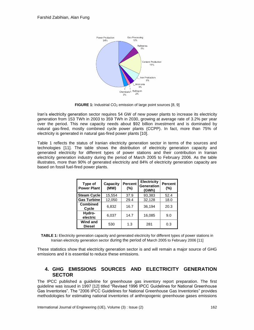
Farshid Zabihian, Alan Fung
International Journal of Engineering (IJE), Volume (3) : Issue (2) 162
FIGURE 1: Industrial CO2 emission of large point sources [8, 9]
Iran’s electricity generation sector requires 54 GW of new power plants to increase its electricity generation from 153 TWh in 2003 to 359 TWh in 2030, growing at average rate of 3.2% per year over the period. This new capacity needs about $92 billion investment and is dominated by natural gas-fired, mostly combined cycle power plants (CCPP). In fact, more than 75% of electricity is generated in natural gas-fired power plants [10]. Table 1 reflects the status of Iranian electricity generation sector in terms of the sources and technologies [11]. The table shows the distribution of electricity generation capacity and generated electricity for different types of power stations and their contribution in Iranian electricity generation industry during the period of March 2005 to February 2006. As the table illustrates, more than 90% of generated electricity and 84% of electricity generation capacity are based on fossil fuel-fired power plants.
Type of Power Plant
Capacity (MW)
Percent (%)
Electricity Generation
(GWh)
Percent (%)
Steam Cycle 15,554 37.9 93,383 52.4
Gas Turbine 12,050 29.4 32,128 18.0
Combined Cycle
6,832 16.7 36,194 20.3
Hydro-electric
6,037 14.7 16,085 9.0
Wind and Diesel
530 1.3 281 0.3
TABLE 1: Electricity generation capacity and generated electricity for different types of power stations in
Iranian electricity generation sector during the period of March 2005 to February 2006 [11]
These statistics show that electricity generation sector is and will remain a major source of GHG emissions and it is essential to reduce these emissions.
4. GHG EMISSIONS SOURCES AND ELECTRICITY GENERATION SECTOR
The IPCC published a guideline for greenhouse gas inventory report preparation. The first guideline was issued in 1997 [12] titled “Revised 1996 IPCC Guidelines for National Greenhouse Gas Inventories”. The “2006 IPCC Guidelines for National Greenhouse Gas Inventories” provides methodologies for estimating national inventories of anthropogenic greenhouse gases emissions

Farshid Zabihian, Alan Fung
International Journal of Engineering (IJE), Volume (3) : Issue (2) 163
and removals by GHG sources and sinks. This guideline categorized GHG production sources into 5 categories [13]: energy; industrial processes and product use; agriculture, forestry and other land use; waste; and others. Based on the 2006 IPCC Guidelines, electricity generation sector is considered to be in category 1-A-1-a-i. The definition of these categories is as follows [13]: 1- Energy: Comprises emissions from combustion and fugitive releases of fuels for energy uses. All GHG emissions from the non-energy consumption of fuels are commonly included under Industrial Processes and Product Use. 1 A - Fuel Combustion Activities: GHG emissions from the intentional oxidation of fuels within a device to generate either heat or mechanical work. 1 A 1 - Energy Industries: Sum of emissions from fuels consumption for power generation industries. 1 A 1 a - Main Activity, Electricity and Heat Production: All emissions from electricity generation, combined heat and power generation, and heat plants that their products are supplied the public. These plants can be in public or private ownership and include on-site use of fuel. 1 A 1 a i – Electricity Generation: GHG emissions from all fuel combustion to generate electricity excluding those from combined heat and power plants.
5. DIFFERENT METHODOLOGIES TO ESTIMATE GHG EMISSIONS
In this section different methods to estimate GHG emissions will be investigated and the estimation for Iranian electricity generation sector will be presented as a case study. In this paper the “2006 IPCC Guidelines for National Greenhouse Gas Inventories” [13] will be used for estimating GHG emissions for Category 1-A-1-a-i. Generally, emission of each GHG is estimated by multiplying fuel consumption by the corresponding emission factor. There are three tiers presented in the 2006 IPCC Guidelines for estimating emissions from fossil fuel combustion for electricity generation. In these tiers fuel consumption and emission factors are considered as follows [13]: Tier 1: fuel consumption from national energy statistics and default emission factors; Tier 2: fuel consumption from national energy statistics and country-specific emission factors; Tier 3: fuel consumption from national energy statistics for different electricity generation technol-ogies and technology-specific emission factors. All tiers use the fuel consumption as the activity data. Thus, this parameter will be defined and then the tiers will be explained. Activity data To estimate GHG emissions from stationary power generation, the activity data are typically the fuel consumption to generate electricity. As it will be elaborated later in this section, these data are sufficient for Tier 1 analysis. In higher tier approaches, additional data are required on fuel characteristics and the power generation technologies. In most of national energy statistics used for GHG emissions estimation, fuels consumption is specified in physical units, such as in tonnes or cubic meters. But in above mentioned tiers, the energy content of consumed fuels is required to estimate GHG emissions. Therefore, the mass or volume units of fuel consumption should be first converted. The fuels energy content can be expressed by two definitions:
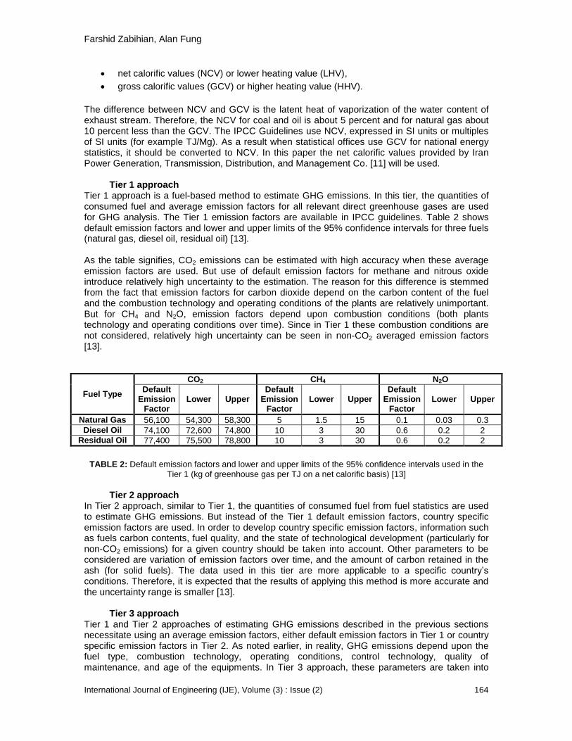
Farshid Zabihian, Alan Fung
International Journal of Engineering (IJE), Volume (3) : Issue (2) 164
net calorific values (NCV) or lower heating value (LHV),
gross calorific values (GCV) or higher heating value (HHV).
The difference between NCV and GCV is the latent heat of vaporization of the water content of exhaust stream. Therefore, the NCV for coal and oil is about 5 percent and for natural gas about 10 percent less than the GCV. The IPCC Guidelines use NCV, expressed in SI units or multiples of SI units (for example TJ/Mg). As a result when statistical offices use GCV for national energy statistics, it should be converted to NCV. In this paper the net calorific values provided by Iran Power Generation, Transmission, Distribution, and Management Co. [11] will be used. Tier 1 approach Tier 1 approach is a fuel-based method to estimate GHG emissions. In this tier, the quantities of consumed fuel and average emission factors for all relevant direct greenhouse gases are used for GHG analysis. The Tier 1 emission factors are available in IPCC guidelines. Table 2 shows default emission factors and lower and upper limits of the 95% confidence intervals for three fuels (natural gas, diesel oil, residual oil) [13]. As the table signifies, CO2 emissions can be estimated with high accuracy when these average emission factors are used. But use of default emission factors for methane and nitrous oxide introduce relatively high uncertainty to the estimation. The reason for this difference is stemmed from the fact that emission factors for carbon dioxide depend on the carbon content of the fuel and the combustion technology and operating conditions of the plants are relatively unimportant. But for CH4 and N2O, emission factors depend upon combustion conditions (both plants technology and operating conditions over time). Since in Tier 1 these combustion conditions are not considered, relatively high uncertainty can be seen in non-CO2 averaged emission factors [13].
Fuel Type
CO2 CH4 N2O
Default Emission
Factor Lower Upper
Default Emission
Factor Lower Upper
Default Emission
Factor Lower Upper
Natural Gas 56,100 54,300 58,300 5 1.5 15 0.1 0.03 0.3
Diesel Oil 74,100 72,600 74,800 10 3 30 0.6 0.2 2
Residual Oil 77,400 75,500 78,800 10 3 30 0.6 0.2 2
TABLE 2: Default emission factors and lower and upper limits of the 95% confidence intervals used in the
Tier 1 (kg of greenhouse gas per TJ on a net calorific basis) [13]
Tier 2 approach In Tier 2 approach, similar to Tier 1, the quantities of consumed fuel from fuel statistics are used to estimate GHG emissions. But instead of the Tier 1 default emission factors, country specific emission factors are used. In order to develop country specific emission factors, information such as fuels carbon contents, fuel quality, and the state of technological development (particularly for non-CO2 emissions) for a given country should be taken into account. Other parameters to be considered are variation of emission factors over time, and the amount of carbon retained in the ash (for solid fuels). The data used in this tier are more applicable to a specific country’s conditions. Therefore, it is expected that the results of applying this method is more accurate and the uncertainty range is smaller [13]. Tier 3 approach Tier 1 and Tier 2 approaches of estimating GHG emissions described in the previous sections necessitate using an average emission factors, either default emission factors in Tier 1 or country specific emission factors in Tier 2. As noted earlier, in reality, GHG emissions depend upon the fuel type, combustion technology, operating conditions, control technology, quality of maintenance, and age of the equipments. In Tier 3 approach, these parameters are taken into
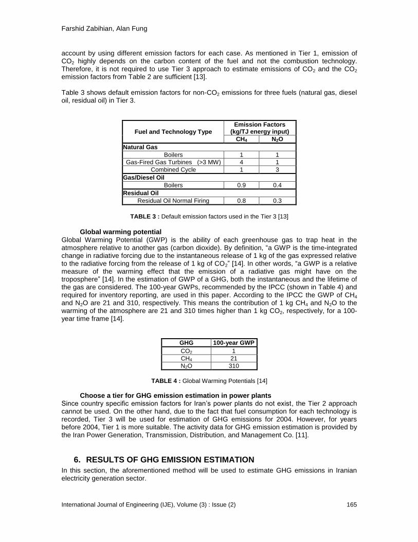
Farshid Zabihian, Alan Fung
International Journal of Engineering (IJE), Volume (3) : Issue (2) 165
account by using different emission factors for each case. As mentioned in Tier 1, emission of CO2 highly depends on the carbon content of the fuel and not the combustion technology. Therefore, it is not required to use Tier 3 approach to estimate emissions of CO2 and the CO2 emission factors from Table 2 are sufficient [13]. Table 3 shows default emission factors for non-CO2 emissions for three fuels (natural gas, diesel oil, residual oil) in Tier 3.
Fuel and Technology Type
Emission Factors (kg/TJ energy input)
CH4 N2O
Natural Gas
Boilers 1 1
Gas-Fired Gas Turbines (>3 MW) 4 1
Combined Cycle 1 3
Gas/Diesel Oil
Boilers 0.9 0.4
Residual Oil
Residual Oil Normal Firing 0.8 0.3
TABLE 3 : Default emission factors used in the Tier 3 [13]
Global warming potential Global Warming Potential (GWP) is the ability of each greenhouse gas to trap heat in the atmosphere relative to another gas (carbon dioxide). By definition, “a GWP is the time-integrated change in radiative forcing due to the instantaneous release of 1 kg of the gas expressed relative to the radiative forcing from the release of 1 kg of CO2” [14]. In other words, “a GWP is a relative measure of the warming effect that the emission of a radiative gas might have on the troposphere” [14]. In the estimation of GWP of a GHG, both the instantaneous and the lifetime of the gas are considered. The 100-year GWPs, recommended by the IPCC (shown in Table 4) and required for inventory reporting, are used in this paper. According to the IPCC the GWP of CH4 and N2O are 21 and 310, respectively. This means the contribution of 1 kg CH4 and N2O to the warming of the atmosphere are 21 and 310 times higher than 1 kg CO2, respectively, for a 100-year time frame [14].
GHG 100-year GWP
CO2 1
CH4 21
N2O 310
TABLE 4 : Global Warming Potentials [14]
Choose a tier for GHG emission estimation in power plants Since country specific emission factors for Iran’s power plants do not exist, the Tier 2 approach cannot be used. On the other hand, due to the fact that fuel consumption for each technology is recorded, Tier 3 will be used for estimation of GHG emissions for 2004. However, for years before 2004, Tier 1 is more suitable. The activity data for GHG emission estimation is provided by the Iran Power Generation, Transmission, Distribution, and Management Co. [11].
6. RESULTS OF GHG EMISSION ESTIMATION
In this section, the aforementioned method will be used to estimate GHG emissions in Iranian electricity generation sector.

Farshid Zabihian, Alan Fung
International Journal of Engineering (IJE), Volume (3) : Issue (2) 166
Table 5 shows the calculation results (electricity generation, fuel consumption, GHG emissions and GHG intensity) for electricity generation by fossil fuel-fired thermal power stations in Iran for the period of March 2005 to February 2006. In this table, greenhouse gas intensity is the ratio of greenhouse gas emissions to generated electricity. This parameter is used to evaluate the performance of electricity generation sector in terms of GHG emissions. Tier 3 approach has been used for this table with default emission factors from Table 2 and Table 3. As shown in the table, the greenhouse gas intensity for steam power plants, gas turbines and combined cycle power plants are 617, 773, and 462 gCO2eq/kWh, respectively with the overall intensity of 610 gCO2eq/kWh for all thermal power plants. It can be seen that combined cycle power plants emit 25% and 40% less GHG compared to steam power plants and gas turbines, respectively. This result is expected because combined cycle power plants have higher efficiency. In this case, the efficiency of steam power plants, gas turbines and combined cycle power plants are 36.5%, 27.8%, and 45.5%, respectively, during the same period. This means 25% and 64% higher efficiency for combined cycles in comparison to steam power plants and gas turbines, respectively.
Power Plant Type
Electricity Generation
(GWh)
Fuel Consumption GHG Emissions (kt/year) GHG Intensity (gCO2eq/
kWh) NG (10
6 m
3)
Diesel (10
6 lit)
Residual Oil(10
6 lit)
NG Diesel Residual
Oil
Steam Cycle 89,574 17,211 43 6,329 35,074 123 20,104 617
Gas Turbine 29,023 8,444 1,819 0 17,227 5,220 0 773
Combined Cycle
36,194 7,204 660 0 14,841 1,894 0 462
Total/Ave 154,791 32,859 2,522 6,329 67,143 7,237 20,104 610
TABLE 5 : GHG emissions in Iran's thermal power plants from March 2005 to February 2006
Regarding average GHG intensity, it should be mentioned that the value shown in Table 5, 610 gCO2eq/kWh, is just for thermal power plants. If whole electricity generation is considered (including hydro-electric power plants) this intensity will be reduced to 570 gCO2eq/kWh. Table 6 shows the GHG emissions and intensity of Iran's electricity generation sector from 1995 to 2005. According to this table, the average GHG intensity was reduced by 13% in this period. One of the reasons for this GHG emission reduction in Iranian electricity generation sector was that in recent years many combined cycle power plants were installed in the country. In fact, in 1999 there was no electricity generation using combined cycles, but in 2005, 20% of total electricity was generated by using these power plants. Moreover, fuel switching from diesel and residual oil to natural gas is another factor for the reduced GHG emissions.
Year
Electricity Generation (GWh)
GHG Emissions (kt)
GHG Intensity (gCO2eq/ kWh)
Thermal Total Thermal Total
2005 157,181 173,547 98,991 630 570
2004 149,103 160,029 90,958 610 568
2003 135,574 146,988 79,631 587 542
2002 126,740 135,177 78,844 622 583
2001 118,890 124,306 75,099 632 604
2000 111,697 115,708 70,863 634 612
1999 101,845 105,187 65,137 640 619
1998 90,474 97,862 57,222 632 585
1997 84,926 92,310 57,470 677 623
1996 77,839 85,825 53,959 693 629
1995 72,046 80,044 52,299 726 653
TABLE 6: GHG emissions and intensity of Iran's electricity generation sector from 1995 to 2005

Farshid Zabihian, Alan Fung
International Journal of Engineering (IJE), Volume (3) : Issue (2) 167
So far the results demonstrated that Iran’s electricity generation sector did a reasonably good job in reducing the GHG intensity in the past 10 years. However, the detailed calculation proved that still there are power plants with extremely high GHG intensity. The detailed estimation of GHG for all Iran’s major power plants (with annual electricity generation of more than 100,000 MWh in 2005) has been preformed [15]. The results showed that the GHG intensity for steam power plants was ranging from 515 to 1125 gCO2eq/kWh. The range for gas turbines and combined cycles were 584-1346 and 428-513 gCO2eq/kWh, respectively [16]. This indicated that there are great potentials for further GHG intensity reduction in the sector [17]. In the remainder of this paper some of these potentials will be discussed.
7. GHG EMISSION REDUCTION SCENARIOS
As mentioned, the electricity production industry has been responsible for a considerable portion of total GHG emissions. Therefore, in the remainder of this paper, GHG emission reduction potentials under different scenarios will be investigated. These scenarios are based on fuel switching and the adoption of advanced power generation systems (based solely on fossil fuels) in electricity generation. Despite the problems associated with fossil fuel-fired power plants, fossil fuels are available on a mid and long-term basis and their continued large-scale and widespread applications in power generation industry are essential in order to maintain current economic growth in the world. The IEA has commented that “numerous technology solutions offer substantial CO2 reduction potentials, including renewable energies, higher efficiency power generation, fossil-fuel use with CO2 capture and storage, nuclear fission, fusion energy, hydrogen, biofuels, fuel cells and efficient energy end use. No single technology can meet this challenge by itself. Different regions and countries will require different combinations of technologies to best serve their needs and best exploit their indigenous resources. The energy systems of tomorrow will rely on a mix of different advanced, clean, efficient technologies for energy supply and use” [18]. Thus, both fossil and non-fossil forms of energy will be needed in the foreseeable future to meet global energy demands. It is, therefore, important that alternative technologies are commercialized to permit the consumption of fossil fuels with significantly reduced GHG emissions and other pollutants.
Based on this, different scenarios to reduce GHG emissions are defined as follows: Scenario number 1: In this scenario, GHG emission reduction potentials by fuel switching will be investigated. Based on this scenario, all power plants will use natural gas as primary fuel instead of their original fuel. But technology of power stations will remain unchanged. Scenario number 2: In the second scenario, there will be fuel switching as well as technology changes. In this scenario, all power stations will be replaced by natural gas combined cycle (NGCC). The size of the alternative NGCC power plant is 505 MW. The plant configuration consists of two gas turbines, a heat recovery steam generator, and a condensing reheat steam turbine. In this work the efficiency of the power plant is considered to be 49% (based on HHV) [19]. Scenario numbers 3 and 4: In order to implement these scenarios all existing power stations will be replaced by solid oxide fuel cell (SOFC) for the third scenario and hybrid SOFC power plants for the fourth scenario. In both cases power plants will be fueled by natural gas. Fuel cells operation is based on direct and continuous conversion of fuel chemical energy into electrical energy in electrochemical process. Because of this direct energy conversion, their efficiencies are usually higher than conventional electricity generation technologies. Fuel cells can be classified by their operating temperature and electrolyte compositions, which dictate their suitability for different applications. Solid oxide fuel cells have high operating
Farshid Zabihian, Alan Fung
International Journal of Engineering (IJE), Volume (3) : Issue (2) 168
temperature (between 600 °C-1000 °C) which makes them especially suited for stationary power generation. SOFCs can use natural gas, syngas from coal, and various biofuels directly due to this high operating temperature, which allow for internal reforming of these fuels within the cells. The SOFC operating temperature is also high enough to allow for integration with gas turbines and/or other bottoming cycles in hybrid power plants. A hybrid SOFC cycle could be any combination of SOFC and gas turbine, steam turbine or combined cycle. There are numerous demonstrational and semi-commercial units of SOFCs installed around the world with different sizes and configurations [20, 21, 22, 23]. But so far, to the authors’ best knowledge, there have been three proof-of-concept SOFC hybrid power plants installed in the world. Siemens claims that it has been successfully demonstrated its pressurized SOFC and gas turbine hybrid system and has two units; a 220 kW at the University of California, Irvine, and a 300 kW unit in Pittsburgh [24, 25]. Also, in 2006 Mitsubishi Heavy Industries, Ltd. (MHI), Japan, claimed that it succeeded in verification testing of a 75 kW SOFC and micro GT hybrid cycle [26]. As mentioned, these two technologies are in development phase and there is no commercial product in the market yet. Therefore, there are no universally accepted configurations for them. For SOFC power generation units, efficiency of 50% to 60% has been reported [27, 28, 29, 30]. In the case of the SOFC hybrid cycle, the efficiency is higher and its range is wider, from 57% to 75% [31, 32, 33, 34, 35, 36]. For this paper the average efficiencies of 55% for the third scenario and 65% for the fourth scenario are considered. Scenario numbers 5 and 6: CO2 capture and storage (CCS) systems are technologies that can be used to reduce CO2 emission by different industries where combustion is part of the process. A major problem of CCS utilization is their high efficiency penalty in power plants. For different types of power plants fueled by oil, natural gas, and coal there are three main techniques that can be applied [37, 38]:
CO2 capture after combustion (post-combustion);
CO2 capture after concentration of flue gas by using pure oxygen in boilers and furnaces
(oxyfuel power plants); and
CO2 capture before combustion (pre-combustion).
The first method is consisted of treating exhaust gases (most likely by chemical absorption) in order to remove, liquefy and store carbon dioxide. This technology is currently expensive and involves significant efficiency penalty. The oxyfuel process increases the CO2 concentration in the plant’s off-gas by combusting fuel with pure oxygen instead of air. In the last method, fuel is first gasified and then CO2 is removed from hydrogen rich fuel. The product of this process is almost pure hydrogen which can be used as a fuel in power plants. In the fifth scenario, CCS is installed in the existing power plants with current technologies. For the last scenario, all existing power plants will be replaced by NGCC plants equipped with CO2 capture system. The CCS system in these scenarios is capable of removing 90% of CO2 from flue gas. But because of consumption of more fuel to compensate plants efficiency reduction, overall, 87% of CO2 can be captured. The output penalty of 10% is considered for both scenarios.
8. GHG EMISSION REDUCTION POTENTIALS IN IRAN
Table 7 shows the energy of consumed fuel, electricity generation, GHG emissions and intensity for existing power plants and six reference scenarios and reduction potentials in each scenario in Iran’s electricity generation sector for the period of March 2005 to February 2006. Again, the focus of this paper is on GHG emission reduction on fossil fuel-fired thermal power plants and other power generation technologies are not considered.
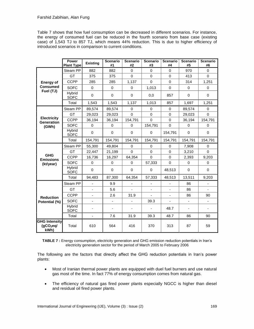
Farshid Zabihian, Alan Fung
International Journal of Engineering (IJE), Volume (3) : Issue (2) 169
Table 7 shows that how fuel consumption can be decreased in different scenarios. For instance, the energy of consumed fuel can be reduced in the fourth scenario from base case (existing case) of 1,543 TJ to 857 TJ, which means 44% reduction. This is due to higher efficiency of introduced scenarios in comparison to current conditions.
Power
Plant Type Existing
Scenario #1
Scenario #2
Scenario #3
Scenario #4
Scenario #5
Scenario #6
Energy of Consumed Fuel (TJ)
Steam PP 882 882 0 0 0 970 0
GT 375 375 0 0 0 413 0
CCPP 285 285 1,137 0 0 314 1,251
SOFC 0 0 0 1,013 0 0 0
Hybrid SOFC
0 0 0 0,0 857 0 0
Total 1,543 1,543 1,137 1,013 857 1,697 1,251
Electricity Generation
(GWh)
Steam PP 89,574 89,574 0 0 0 89,574 0
GT 29,023 29,023 0 0 0 29,023 0
CCPP 36,194 36,194 154,791 0 0 36,194 154,791
SOFC 0 0 0 154,791 0 0 0
Hybrid SOFC
0 0 0 0 154,791 0 0
Total 154,791 154,791 154,791 154,791 154,791 154,791 154,791
GHG Emissions
(kt/year)
Steam PP 55,300 49,804 0 0 0 7,908 0
GT 22,447 21,199 0 0 0 3,210 0
CCPP 16,736 16,297 64,354 0 0 2,393 9,203
SOFC 0 0 0 57,333 0 0 0
Hybrid SOFC
0 0 0 0 48,513 0 0
Total 94,483 87,300 64,354 57,333 48,513 13,511 9,203
Reduction Potential (%)
Steam PP - 9.9 - - - 86 -
GT - 5.6 - - - 86 -
CCPP - 2.6 31.9 - - 86 90
SOFC - - - 39.3 - - -
Hybrid SOFC
- - - - 48.7 - -
Total - 7.6 31.9 39.3 48.7 86 90
GHG Intensity (gCO2eq/
kWh) Total 610 564 416 370 313 87 59
TABLE 7 : Energy consumption, electricity generation and GHG emission reduction potentials in Iran’s
electricity generation sector for the period of March 2005 to February 2006
The following are the factors that directly affect the GHG reduction potentials in Iran’s power plants:
Most of Iranian thermal power plants are equipped with duel fuel burners and use natural gas most of the time. In fact 77% of energy consumption comes from natural gas.
The efficiency of natural gas fired power plants especially NGCC is higher than diesel and residual oil fired power plants.
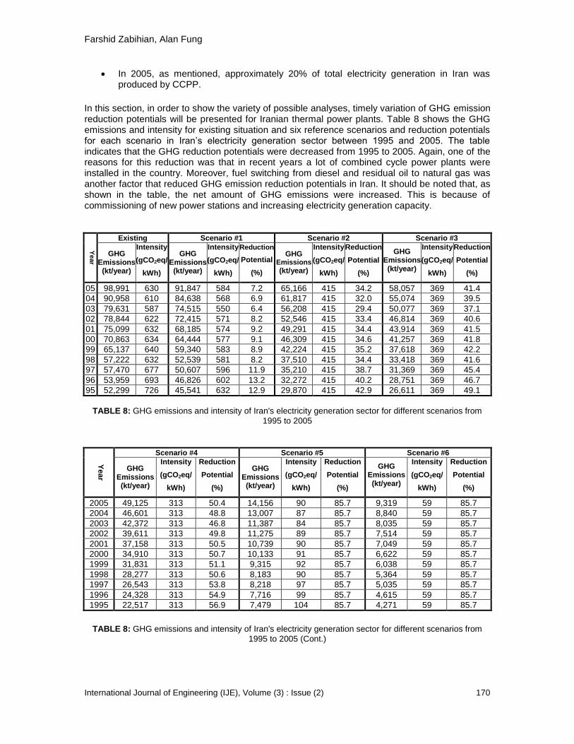
Farshid Zabihian, Alan Fung
International Journal of Engineering (IJE), Volume (3) : Issue (2) 170
In 2005, as mentioned, approximately 20% of total electricity generation in Iran was produced by CCPP.
In this section, in order to show the variety of possible analyses, timely variation of GHG emission reduction potentials will be presented for Iranian thermal power plants. Table 8 shows the GHG emissions and intensity for existing situation and six reference scenarios and reduction potentials for each scenario in Iran’s electricity generation sector between 1995 and 2005. The table indicates that the GHG reduction potentials were decreased from 1995 to 2005. Again, one of the reasons for this reduction was that in recent years a lot of combined cycle power plants were installed in the country. Moreover, fuel switching from diesel and residual oil to natural gas was another factor that reduced GHG emission reduction potentials in Iran. It should be noted that, as shown in the table, the net amount of GHG emissions were increased. This is because of commissioning of new power stations and increasing electricity generation capacity.
Year
Existing Scenario #1 Scenario #2 Scenario #3
GHG Emissions (kt/year)
Intensity
(gCO2eq/
kWh)
GHG Emissions (kt/year)
Intensity
(gCO2eq/
kWh)
Reduction
Potential
(%)
GHG Emissions
(kt/year)
Intensity
(gCO2eq/
kWh)
Reduction
Potential
(%)
GHG Emissions (kt/year)
Intensity
(gCO2eq/
kWh)
Reduction
Potential
(%)
05 98,991 630 91,847 584 7.2 65,166 415 34.2 58,057 369 41.4
04 90,958 610 84,638 568 6.9 61,817 415 32.0 55,074 369 39.5
03 79,631 587 74,515 550 6.4 56,208 415 29.4 50,077 369 37.1
02 78,844 622 72,415 571 8.2 52,546 415 33.4 46,814 369 40.6
01 75,099 632 68,185 574 9.2 49,291 415 34.4 43,914 369 41.5
00 70,863 634 64,444 577 9.1 46,309 415 34.6 41,257 369 41.8
99 65,137 640 59,340 583 8.9 42,224 415 35.2 37,618 369 42.2
98 57,222 632 52,539 581 8.2 37,510 415 34.4 33,418 369 41.6
97 57,470 677 50,607 596 11.9 35,210 415 38.7 31,369 369 45.4
96 53,959 693 46,826 602 13.2 32,272 415 40.2 28,751 369 46.7
95 52,299 726 45,541 632 12.9 29,870 415 42.9 26,611 369 49.1
TABLE 8: GHG emissions and intensity of Iran's electricity generation sector for different scenarios from
1995 to 2005
Year
Scenario #4 Scenario #5 Scenario #6
GHG Emissions (kt/year)
Intensity
(gCO2eq/
kWh)
Reduction
Potential
(%)
GHG Emissions (kt/year)
Intensity
(gCO2eq/
kWh)
Reduction
Potential
(%)
GHG Emissions (kt/year)
Intensity
(gCO2eq/
kWh)
Reduction
Potential
(%)
2005 49,125 313 50.4 14,156 90 85.7 9,319 59 85.7
2004 46,601 313 48.8 13,007 87 85.7 8,840 59 85.7
2003 42,372 313 46.8 11,387 84 85.7 8,035 59 85.7
2002 39,611 313 49.8 11,275 89 85.7 7,514 59 85.7
2001 37,158 313 50.5 10,739 90 85.7 7,049 59 85.7
2000 34,910 313 50.7 10,133 91 85.7 6,622 59 85.7
1999 31,831 313 51.1 9,315 92 85.7 6,038 59 85.7
1998 28,277 313 50.6 8,183 90 85.7 5,364 59 85.7
1997 26,543 313 53.8 8,218 97 85.7 5,035 59 85.7
1996 24,328 313 54.9 7,716 99 85.7 4,615 59 85.7
1995 22,517 313 56.9 7,479 104 85.7 4,271 59 85.7
TABLE 8: GHG emissions and intensity of Iran's electricity generation sector for different scenarios from
1995 to 2005 (Cont.)

Farshid Zabihian, Alan Fung
International Journal of Engineering (IJE), Volume (3) : Issue (2) 171
9. CONCLUSION
The first part of this paper showed the importance of preparation of GHG inventory report for electricity generation sector. The results demonstrated that Iran’s electricity generation sector did a reasonably good job in reducing the GHG intensity in the past 10 years, with 13% overall reduction. However, the detailed calculation pointed out that still there are power plants with extremely high GHG emission intensity. This indicated that there are great potentials for further GHG emission reduction in the sector. In the remainder of the paper, the GHG emission reduction potentials were investigated through six scenarios. The results illustrated that there are considerable GHG emission reduction potentials in Iranian electricity generation sector. Implementation of the scenarios can help the country in sustainable development. Moreover, it could be economically beneficial due to the possibility of selling Carbon Credit to Annex I parties of the Kyoto Protocol.
10. ACKNOWLEDGEMENTS
The authors gratefully acknowledge the financial support provided by the Natural Sciences and Engineering Research Council of Canada (NSERC) through the Discovery Grants (DG).
11. REFERENCE
1. IPCC. “Climate Change 2007: Synthesis Report, An Assessment of the Intergovernmental Panel on
Climate Change”. 2007.
2. IPCC. “Third Assessment Report:Climate Change”. Working Group I of the IPCC, 2001.
3. UNFCC. “Article 2, The United Nations Framework Convention on Climate Change”. 2005.
4. UNFCC. “Kyoto Protocol to the United Nations Framework Convention on Climate Change
(UNFCCC)”. 1997.
5. http://unfccc.int/kyoto_protocol/background/status_of_ratification/items/2613.php (May 10, 2009).
6. IPCC. “Third Assessment Report:Climate Change”. Working Group I of the IPCC”, 2001.
7. International Energy Agency, “World Energy Outlook”. 2006.
8. J. Gale. “Overview of Sources, Potential, Transport and Geographical Distribution of Storage
Possibilities”. IPCC Workshop on Carbon Capture and Storage, Regina, Canada, 2002.
9. N. Bauer. “Carbon Capturing and Sequestration An Option to Buy Time?”. Doctor Rerum Politicarum,
University Potsdam Faculty of Economics and Social Sciences, 2005.
10. International Energy Agency, “World Energy Outlook 2005: Middle East and North Africa insights”.
2005.
11. Iran Power Generation, Transmission, Distribution, Management Co. “Detailed Statistic of Iran’s
electricity industry (2005 and 06)”. Second Volume: Electricity Generatoin Sector, 2007.

Farshid Zabihian, Alan Fung
International Journal of Engineering (IJE), Volume (3) : Issue (2) 172
12. J. T. Houghton, L. G. Meira Filho, B. Lim, K. Tréanton, I. Mamaty, Y. Bonduki, D. J. Griggs, B. A.
Callander, Intergovernmental Panel on Climate Change (IPCC). “Revised 1996 IPCC Guidelines for
National Greenhouse Inventories”. IPCC/OECD/IEA, Paris, France, 1997.
13. H. S. Eggleston, L. Buendia, K. Miwa, T. Ngara, K. Tanabe. The Intergovernmental Panel on Climate
Change (IPCC), “IPCC Guidelines for National Greenhouse Gas Inventories (2006). The National
Greenhouse Gas Inventories Programme”. IGES, Japan, Volume 2, Energy, 2006.
14. Environment Canada. “Canada’s Greenhouse Gas Inventory 1990–2004”. Greenhouse Gas Division
Environment Canada, 2006.
15. F. Zabihian, A. Fung. “Estimation of Greenhouse Gas Emissions in Iran’s Electricity Generation
Sector”. In Proceedings of the 22nd International Power Systems Conference, Tehran, Iran, 2007.
16. F. Zabihian, A. Fung. “Greenhouse Gas Emissions Calculation Methodology in Thermal Power Plants
- Case Study of Iran and Comparison with Canada”. In Proceedings of the ASME Power conference
2008, Florida, USA, 2008.
17. F. Zabihian, A. Fung. “Thermal Power Plants Greenhouse Gas Emissions”. In Proceedings of the Fuel,
Energy and Environmental Congress, Tehran, Iran, 2008.
18. IEA. “Energy Technology: Facing the Climate Challenge”. IEA Governing Board, 2003.
19. P. L. Spath, M. K. Mann. “Life Cycle Assessment of a Natural Gas Combined- Cycle Power Generation
System”. National Renewable Energy Laboratory (NREL), Department of Energy Laboratory, U.S.,
2000.
20. S. C. Singhal, K. Kendall. “High temperature solid oxide fuel cell, fundumental, design and
applications”. 2006.
21. S. C. Singhal. “Solid oxide fuel cells for stationary, mobile, and military applications”. Solid State
Ionics; 152-153:405-410, 2002.
22. “Fuel cell handbook”, EG&G Technical Services, Inc., (2004).
23. M. C. Williams, J. P. Strakey, W. A. Surdoval, L. C. Wilson. “Solid oxide fuel cell technology
development in the U.S.”. Solid State Ionics, 177:2039-2044, 2006.
24. S. E. Veyo, L. A. Shockling, J. T. Dederer, J. E. Gillett, W. L. Lundberg. “Tubular solid oxide fuel
cell/gas turbine hybrid cycle power systems: Status”. Journal of Engineering for Gas Turbines and
Power, 124:845-849, 2002.
25. S. E. Veyo, S. D. Vora, K. P. Litzinger, W. L. Lundberg. “Status of pressurized SOFC/GAS turbine
power system development at Siemens Westinghouse”. Proceedings of the ASME Turbo Expo,
Amsterdam, Netherlands, 2002.
26. http://www.mhi.co.jp/en/news/sec1/200608041128.html (May 10, 2009).
27. L. Petruzzi, S. Cocchi, F. Fineschi. “A global thermo-electrochemical model for SOFC systems design
and engineering”. Journal of Power Sources, 118:96-107, 2003.

Farshid Zabihian, Alan Fung
International Journal of Engineering (IJE), Volume (3) : Issue (2) 173
28. T. Shimada, T. Kato, Y. Tanaka. “Numerical analysis of thermal behavior of small solid oxide fuel cell
systems”. Journal of Fuel Cell Science and Technology, 4:299-307, 2007.
29. S. Campanari. “Carbon dioxide separation from high temperature fuel cell power plants”. Journal of
Power Sources, 112:273-289, 2002.
30. S. Campanari. “Thermodynamic model and parametric analysis of a tubular SOFC module”. Journal of
Power Sources, 92:26-34, 2001.
31. F. Calise, M. Dentice d’Accadia, A. Palombo, L. Vanoli. “Simulation and exergy analysis of a hybrid
Solid Oxide Fuel Cell (SOFC)–Gas Turbine System”. Energy, 31:3278-3299, 2006.
32. S. Campanari. “Carbon dioxide separation from high temperature fuel cell power plants”. Journal of
Power Sources, 112:273-289, 2002.
33. S. H. Chan. “Modeling of simple hybrid solid oxide fuel cell and gas turbine power plant”. Journal of
Power Sources, 109:111-120, 2002.
34. P. Kuchonthara, S. Bhattacharya, A. Tsutsumi. “Energy recuperation in solid oxide fuel cell (SOFC)
and gas turbine (GT) combined system”. Journal of Power Sources, 117:7-13, 2003.
35. J. Palsson, A. Selimovic, L. Sjunnesson. “Combined solid oxide fuel cell and gas turbine systems for
efficient power and heat generation”. Journal of Power Sources, 86:442-448, 2000.
36. T. W. Song, J. L. Sohn, J. H. Kim, T. S. Kim, S. T. Ro, K. Suzuki. “Performance analysis of a tubular
solid oxide fuel cell/micro gas turbine hybrid power system based on a quasi-two dimensional model”.
Journal of Power Sources, 142:30-42, 2005.
37. K. Riahi, E. S. Rubin, L. Schrattenholzer. “Prospects for carbon capture and sequestration
technologies assuming their technological learning”. In Proceedings of the 6th International
Greenhouse Gas Control Technologies, Kyoto, Japan, 2003.
38. B. Metz, O. Davidson, H. C. de Coninck, M. Loos, L. A. Meyer. “IPCC Special Report on Carbon
Dioxide Capture and Storage”. Working Group III of the Intergovernmental Panel on Climate Change.
Cambridge University Press, UK, 2005.

L. Khezzar, A. C. Seibi & A. Goharzadeh
International Journal of Engineering (IJE), Volume (3) : Issue (2) 174
Water Sloshing in Rectangular Tanks – An Experimental Investigation & Numerical Simulation
Lyes Khezzar [email protected] Mechanical Engineering Petroleum Institute, P.O. Box 2533 Abu Dhabi, UAE
Abdennour Seibi [email protected] Mechanical Engineering Petroleum Institute, P.O. Box 2533 Abu Dhabi, UAE
Afshin Goharzadeh [email protected] Mechanical Engineering Petroleum Institute, P.O. Box 2533 Abu Dhabi, UAE
ABSTRACT
This paper presents the steps involved in designing a test rig to study water sloshing phenomenon in a 560 x 160 x 185 mm PVC rectangular container subjected to sudden (impulsive) impact. The design encompasses the construction of the testing facility and the development of a proper data acquisition system capable of capturing the behavior of pre- and post impact water motion inside the tank. Fluid motion was recorded using a video camera for flow visualization purpose. Two water levels of 50 and 75% full as well as two driving weights of 2.5 and 4.5 kg were used. The experimental study was supplemented by a computational fluid dynamics study to mimic the fluid motion inside the tank. Examination of CFD capability to predict the behavior of the free surface of the fluid during the container initial motion and after impact is the focus of this paper. The flow fields, obtained using the numerical code, are in reasonable agreement with those from experiments. Both experimental and numerical results indicated the presence of a single traveling wave before impact, contrary to what was observed in previous studies. Keywords: water sloshing, computational fluid dynamics, flow visualization.
1. INTRODUCTION
The problem of water sloshing in closed containers has been the subject of many studies over the past few decades. This phenomenon can be described as a free surface movement of the contained fluid due to sudden loads. Olsen [1] classified the free surface fluid motion in three different slosh modes consisting of i) lateral sloshing, ii) vertical sloshing, and iii) rotational sloshing (Swirling). Sloshing is a phenomenon that can be found in a wide variety of industrial

L. Khezzar, A. C. Seibi & A. Goharzadeh
International Journal of Engineering (IJE), Volume (3) : Issue (2) 175
applications such as Liquefied Natural Gas (LNG) carriers and their new design, rockets and airplanes fuel reservoirs and road tankers.
The design of this equipment requires detailed understanding of liquid motion during sloshing. Sloshing can be the result of external forces due to acceleration/deceleration of the containment body. Of particular concern is the pressure distribution on the wall of the container reservoir and its local temporal peaks that can reach as in road tankers twice the rigid load value. In road tankers, the free liquid surface may experience large excursions for even very small motions of the container leading to stability problems. Several studies were conducted on sloshing of fluids and the extensive review by Ibrahim et al. [2] and Ibrahim [3] provide a thorough review of the subject liquid sloshing dynamics. Initial work started in the early 1960’s with the study of the influence of liquid propellant sloshing on the flight performance of jet propelled vehicles. Chwang & Wang [4] applied nonlinear theory to calculate the pressure force in accelerating rectangular and circular container. It was found that during the initial stage of the impulsive motion, no traveling free-surface waves are present and the fluid simply piles up on one side of the container. Moreover, Popov et al. [5, 6] studied the effect of acceleration and curvature on the fluid motion in rectangular containers and observed that the dynamic coefficient is influenced by the aspect ratio of fluid height to length. The study revealed that maximum sloshing occurs in square containers with 30 – 60% fluid level and that maximum forces occur at a fluid level ranging between 75 – 93%. A similar study conducted by Ye and Birk [7] investigated the pressure variation at the walls of a horizontal cylindrical vessel during and after impact where fluid sloshing takes place at fluid levels less than 95% full. The study revealed that the pressure in the tank increases as the fluid level inside the tank increases. Faltinsen et al. [8] studied the transient loads on sloshing tanks and observed five distinct transient phases with different amplitudes. Chen and Chiang [9] conducted a simulation study on a simple two-dimensional rectangular tank with rigid walls subjected to horizontal and vertical accelerations using an inviscid and incompressible fluid to examine the nonlinear behavior of fluid motion. The study revealed that the fundamental frequency of the flow is strictly dependent on tank width and fluid depth. The effect of fluid viscosity was studied by Faltinsen and Rognebakke [10] and revealed that viscosity becomes prominent in small amplitude excitations and high fluid levels. Moreover, Bass et al. [11] found that viscosity has a minor effect on sloshing with large excitation amplitudes.
The traditional approaches that have been used to assess sloshing loads include linear and nonlinear potential flow theory, direct experimentation on scaled models and more recently the use of Computational Fluid Dynamics (CFD) investigated by Godderidge et al. [12, 13]. The results showed that the sloshing natural frequency and the inertia of the system are affected by the fluid level. Potential flow theory has some limitations and cannot model fluid fragmentation or merging. CFD is thus increasingly being considered as a viable tool for the study of such flows and is currently being tested and validated as a design method as described by Celebi and Akyildiz [14], Kassisnos and Prusa [15] and Ibrahim [2]. A comparative study, conducted by Cariou and Casella [16], has established that non-impulsive phenomena are correctly simulated but impacts and pressure peaks are still far more difficult to assess and need improvement. The present work focuses on the liquid flow dynamics inside a model accelerating rectangular container subjected to a sudden (impulsive) impact. The container is meant to represent a road tanker in motion and suddenly colliding with another object resulting in an impact and sloshing of the fluid inside it. The study involves experimental flow visualization and CFD modeling based on a two-dimensional geometry using a commercial CFD package. The next two sections contain the experimental set up, measuring, image processing, and computational techniques. These are followed by a result and discussion section and a conclusion.
2. EXPERIMENTAL STUDY

L. Khezzar, A. C. Seibi & A. Goharzadeh
International Journal of Engineering (IJE), Volume (3) : Issue (2) 176
The experimental study aims at capturing the fluid motion before and after impact through visualization. Figure 1 shows a solid model and the actual experimental set up with proper data acquisition system. The test rig consists of an acrylic rectangular tank installed with proper instrumentation for data collection before and after impact. Measurements related to the tank displacement using proximity sensors (Omron E2A-M12) from which the tank speed and acceleration are determined as well as water sloshing behavior through visualization were recorded. Due to the high accuracy of the proximity sensor, the experimental error on time and space measurements are estimated to be less than 1%. Tank motion was recorded at i) the beginning of the accelerated motion, ii) while moving, and iii) after impact using a digital camera of 7.2 Mega pixels, which can capture up to 30 frames per second, and two Light Emitting Diodes (LEDs). The two LEDs were used as a trigger indicator of the release of the tank at the beginning of the experiment and tank impact when it hits the backstop at the end of the motion. Adjustable obstacles (bars) were aligned on the side of the track path where the first 14 bars have a center-to-center distance of 20 mm and the other 8 bars have a center-to-center distance of 50 mm (see Figure 1). Two magnets were installed on the impact wall in order to stop bouncing of the tank after it hits the stopper. A data acquisition system using an interface card (NI PCI-6221) was designed to record the feedback signals from all the sensors used for measurement.
a) Solid model of experimental set-up
b) Actual experimental set-up
FIGURE 1: Experimental setup and data acquisition system
2.1 Testing Procedure
The experimental set up, shown in Figure 1, consists of a rectangular Perspex container (175x175x550 mm) filled with water, the working fluid, and seated on a trolley that runs
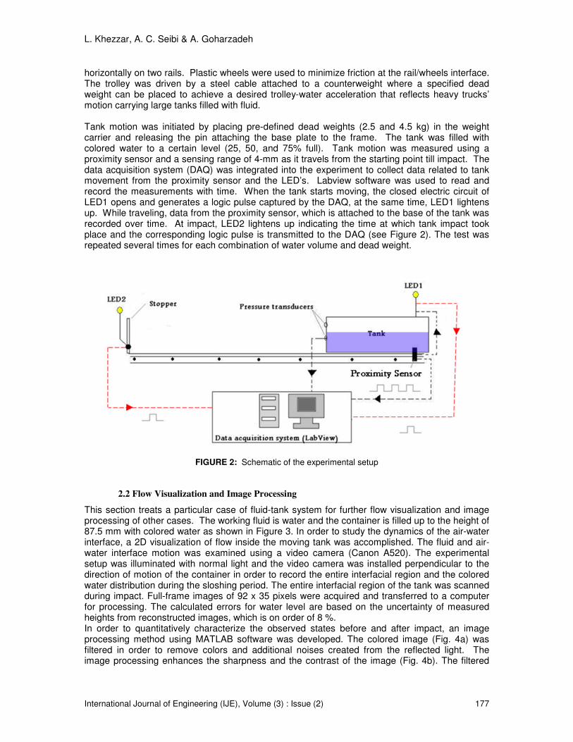
L. Khezzar, A. C. Seibi & A. Goharzadeh
International Journal of Engineering (IJE), Volume (3) : Issue (2) 177
horizontally on two rails. Plastic wheels were used to minimize friction at the rail/wheels interface. The trolley was driven by a steel cable attached to a counterweight where a specified dead weight can be placed to achieve a desired trolley-water acceleration that reflects heavy trucks’ motion carrying large tanks filled with fluid. Tank motion was initiated by placing pre-defined dead weights (2.5 and 4.5 kg) in the weight carrier and releasing the pin attaching the base plate to the frame. The tank was filled with colored water to a certain level (25, 50, and 75% full). Tank motion was measured using a proximity sensor and a sensing range of 4-mm as it travels from the starting point till impact. The data acquisition system (DAQ) was integrated into the experiment to collect data related to tank movement from the proximity sensor and the LED’s. Labview software was used to read and record the measurements with time. When the tank starts moving, the closed electric circuit of LED1 opens and generates a logic pulse captured by the DAQ, at the same time, LED1 lightens up. While traveling, data from the proximity sensor, which is attached to the base of the tank was recorded over time. At impact, LED2 lightens up indicating the time at which tank impact took place and the corresponding logic pulse is transmitted to the DAQ (see Figure 2). The test was repeated several times for each combination of water volume and dead weight.
FIGURE 2: Schematic of the experimental setup
2.2 Flow Visualization and Image Processing
This section treats a particular case of fluid-tank system for further flow visualization and image processing of other cases. The working fluid is water and the container is filled up to the height of 87.5 mm with colored water as shown in Figure 3. In order to study the dynamics of the air-water interface, a 2D visualization of flow inside the moving tank was accomplished. The fluid and air-water interface motion was examined using a video camera (Canon A520). The experimental setup was illuminated with normal light and the video camera was installed perpendicular to the direction of motion of the container in order to record the entire interfacial region and the colored water distribution during the sloshing period. The entire interfacial region of the tank was scanned during impact. Full-frame images of 92 x 35 pixels were acquired and transferred to a computer for processing. The calculated errors for water level are based on the uncertainty of measured heights from reconstructed images, which is on order of 8 %. In order to quantitatively characterize the observed states before and after impact, an image processing method using MATLAB software was developed. The colored image (Fig. 4a) was filtered in order to remove colors and additional noises created from the reflected light. The image processing enhances the sharpness and the contrast of the image (Fig. 4b). The filtered
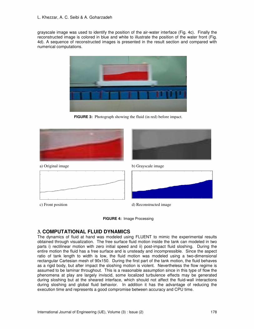
L. Khezzar, A. C. Seibi & A. Goharzadeh
International Journal of Engineering (IJE), Volume (3) : Issue (2) 178
grayscale image was used to identify the position of the air-water interface (Fig. 4c). Finally the reconstructed image is colored in blue and white to illustrate the position of the water front (Fig. 4d). A sequence of reconstructed images is presented in the result section and compared with numerical computations.
FIGURE 3: Photograph showing the fluid (in red) before impact.
a) Original image b) Grayscale image
c) Front position d) Reconstructed image
FIGURE 4: Image Processing
3. COMPUTATIONAL FLUID DYNAMICS The dynamics of fluid at hand was modeled using FLUENT to mimic the experimental results obtained through visualization. The free surface fluid motion inside the tank can modeled in two parts i) rectilinear motion with zero initial speed and ii) post-impact fluid sloshing. During the entire motion the fluid has a free surface and is unsteady and incompressible. Since the aspect ratio of tank length to width is low, the fluid motion was modeled using a two-dimensional rectangular Cartesian mesh of 90x150. During the first part of the tank motion, the fluid behaves as a rigid body, but after impact the sloshing motion is violent. Nevertheless the flow regime is assumed to be laminar throughout. This is a reasonable assumption since in this type of flow the phenomena at play are largely inviscid, some localized turbulence effects may be generated during sloshing but at the sheared interface, which should not affect the fluid-wall interactions during sloshing and global fluid behavior. In addition it has the advantage of reducing the execution time and represents a good compromise between accuracy and CPU time.

L. Khezzar, A. C. Seibi & A. Goharzadeh
International Journal of Engineering (IJE), Volume (3) : Issue (2) 179
The flow is considered incompressible, laminar and unsteady. The modeling of this type of
motion which includes a moving frame denoted by 0ix
attached to the tank relative to an inertial frame, was done using the body force approach described by Godderidge et al [13] and Kassinos and Prusa [15]. The effects of the linear acceleration of the tank on the fluid particles inside it were introduced into the governing equations as body forces:
0i i ig g r= − &&&&&&&& (1)
The relationship between the moving coordinate system and inertial frame is given by:
oi i ix x r= − (2)
The conservation equations of momentum and mass within the moving frame of reference are thus written
as:
2
0 0 00 0
0 0 0
1n n n
i ij n
i n i oj
u u upu g
t x x x x
µδ
ρ ρ
∂ ∂ ∂∂+ = − + +
∂ ∂ ∂ ∂ ∂ (3)
0
0
0i
i
u
x
∂=
∂
Where p is the pressure, µ
is the fluid viscosity, 0iu
is the velocity vector, 0ig
is the total net
body force, ig is the body force within the moving frame and i
r&&&&&&&&is the inertia force resulting from
the motion of the tank. The acceleration ir&&&&&&&&
was calculated from the measured motion of the tank.
The vector ir
denotes the position of the moving frame attached to the tank with respect to the inertial frame of reference. The solution will therefore consist of solving the equations relative to the inertial frame with modified body forces that result from the acceleration of the tank. For this particular case two body forces were taken into account, the gravity in the vertical direction and a horizontal one due to the acceleration of the tank. The horizontal body-force was set to zero for the periods at and after impact. In addition, the absolute velocity of the fluid was modified at impact and set to:
0i i iu u r= + &&&& (4)
Where oiu denotes the fluid velocity field relative to the moving frame calculated before impact
and ir&&&&
is the velocity of the tank at impact. This change is an instantaneous jump and leads to the
strong nonlinear features of the slow behavior after impact. The velocity ir&&&&
was calculated from the measured motion of the tank. The integration time is for 4 seconds and the time step was chosen constant and equal to 0.01 second. This type of flow involves two fluids air and water and a shared interface or free surface. The Volume of Fluid Method (VOF) of Hirt and Nichols [18] is used to track the variation of the interface by solving the continuity or advection equation for the volume fraction of the secondary phase given by:
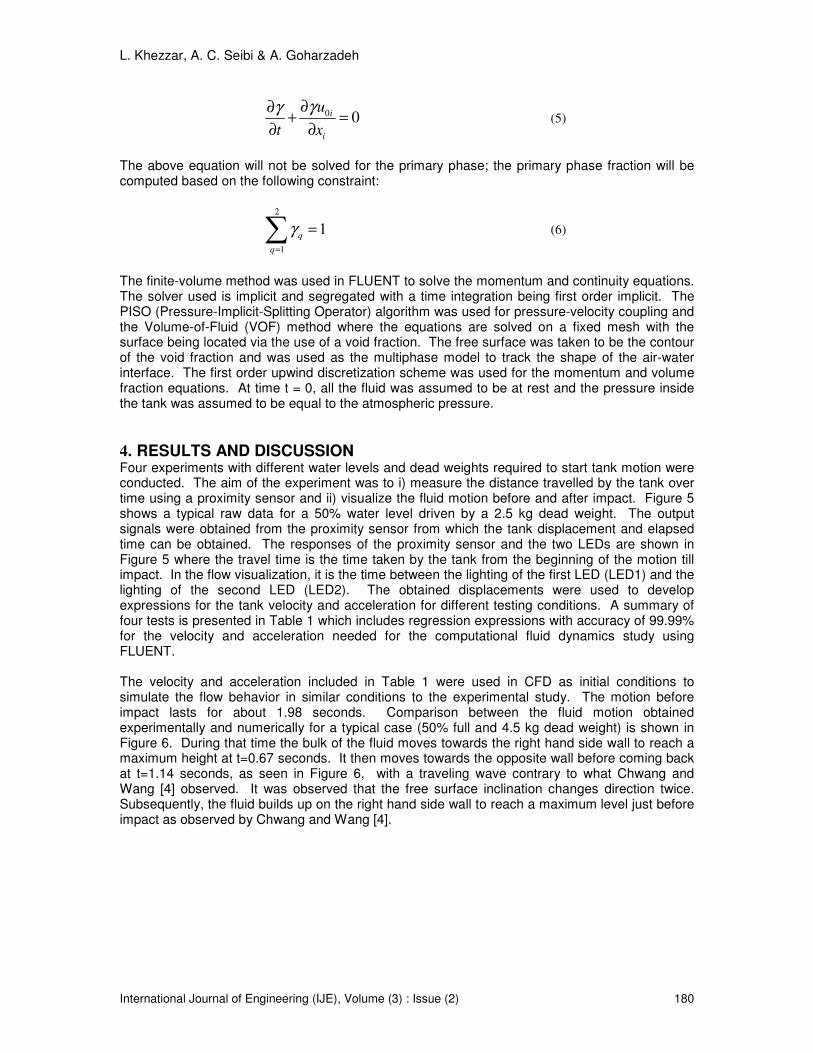
L. Khezzar, A. C. Seibi & A. Goharzadeh
International Journal of Engineering (IJE), Volume (3) : Issue (2) 180
0 0i
i
u
t x
γγ ∂∂+ =
∂ ∂ (5)
The above equation will not be solved for the primary phase; the primary phase fraction will be computed based on the following constraint:
2
1
1q
q
γ=
=∑ (6)
The finite-volume method was used in FLUENT to solve the momentum and continuity equations. The solver used is implicit and segregated with a time integration being first order implicit. The PISO (Pressure-Implicit-Splitting Operator) algorithm was used for pressure-velocity coupling and the Volume-of-Fluid (VOF) method where the equations are solved on a fixed mesh with the surface being located via the use of a void fraction. The free surface was taken to be the contour of the void fraction and was used as the multiphase model to track the shape of the air-water interface. The first order upwind discretization scheme was used for the momentum and volume fraction equations. At time t = 0, all the fluid was assumed to be at rest and the pressure inside the tank was assumed to be equal to the atmospheric pressure.
4. RESULTS AND DISCUSSION Four experiments with different water levels and dead weights required to start tank motion were conducted. The aim of the experiment was to i) measure the distance travelled by the tank over time using a proximity sensor and ii) visualize the fluid motion before and after impact. Figure 5 shows a typical raw data for a 50% water level driven by a 2.5 kg dead weight. The output signals were obtained from the proximity sensor from which the tank displacement and elapsed time can be obtained. The responses of the proximity sensor and the two LEDs are shown in Figure 5 where the travel time is the time taken by the tank from the beginning of the motion till impact. In the flow visualization, it is the time between the lighting of the first LED (LED1) and the lighting of the second LED (LED2). The obtained displacements were used to develop expressions for the tank velocity and acceleration for different testing conditions. A summary of four tests is presented in Table 1 which includes regression expressions with accuracy of 99.99% for the velocity and acceleration needed for the computational fluid dynamics study using FLUENT. The velocity and acceleration included in Table 1 were used in CFD as initial conditions to simulate the flow behavior in similar conditions to the experimental study. The motion before impact lasts for about 1.98 seconds. Comparison between the fluid motion obtained experimentally and numerically for a typical case (50% full and 4.5 kg dead weight) is shown in Figure 6. During that time the bulk of the fluid moves towards the right hand side wall to reach a maximum height at t=0.67 seconds. It then moves towards the opposite wall before coming back at t=1.14 seconds, as seen in Figure 6, with a traveling wave contrary to what Chwang and Wang [4] observed. It was observed that the free surface inclination changes direction twice. Subsequently, the fluid builds up on the right hand side wall to reach a maximum level just before impact as observed by Chwang and Wang [4].

L. Khezzar, A. C. Seibi & A. Goharzadeh
International Journal of Engineering (IJE), Volume (3) : Issue (2) 181
FIGURE 5: Pulse curves for 50% full water level and 2.5 kg dead weight.
Characteristics/case Case 1 Case 2 Case 3 Case 4
Water level (%) 50 50 75 75
Mass used (kg) 2.5 4.5 2.5 4.5
Displacement (m) x(t) = 0.218t1.85
x(t) = 0.407t1.89
x(t) = 0.180t1.84
x(t) = 0.352t1.90
Velocity (m/s) v(t) = 0.0.403t0.85
v(t) = 0.768t0.89
v(t) = 0.33t0.84
v(t) = 0.670t0.90
Acceleration (m/s2) a(t) = 0.34t
-0.15 a(t) = 0.68t
-0.11 a(t) = 0.277t
-0.16 a(t) = 0.605t
-0.10
Travel time tr (sec) 2.82 1.98 3.14 2.12
Terminal velocity
v(tr) (m/s)
0.969 1.41 0.864 1.32
TABLE 1: Cases considered in the experiment with their corresponding results
The experimental profiles compare well with the CFD results; both show the build up against the right, left then right – wall again of the fluid. At impact the fluid exhibits a violent sudden motion forward moving along the opposite vertical wall, around the top left corner and along the ceiling at t=2.17 seconds. At t=2.44 seconds the fluid accumulates in the left half of the container with large surface excursions of fluid and a displaced center of mass, before moving back to the right hand side with subsequent oscillations left-right. The CFD results show some discrepancies with the experimental photographs but the agreement is qualitatively encouraging knowing that the CFD model is two-dimensional and based on laminar flow. The CFD calculations show air entrapped within the bulk of the fluid. The experimental results do not show this entrapment and may due to slow speed of the camera used. The fluid height on the right tank wall was traced experimentally and numerically during the pre- and post impact. Comparison between the simulation and experimental results showed a good agreement. The measured points are nearly similar to the simulated ones especially before impact. However, both results showed some discrepancies after impact due to minor bouncing of the tank (see Figure 7).
Experimental Results Numerical Results
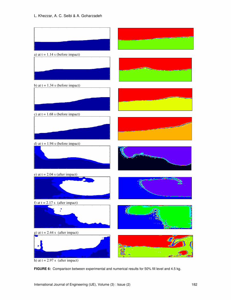
L. Khezzar, A. C. Seibi & A. Goharzadeh
International Journal of Engineering (IJE), Volume (3) : Issue (2) 182
a) at t = 1.14 s (before impact)
b) at t = 1.34 s (before impact)
c) at t = 1.68 s (before impact)
d) at t = 1.94 s (before impact)
e) at t = 2.04 s (after impact)
f) at t = 2.17 s (after impact)
g) at t = 2.44 s (after impact)
h) at t = 2.97 s (after impact)
FIGURE 6: Comparison between experimental and numerical results for 50% fill level and 4.5 kg.

L. Khezzar, A. C. Seibi & A. Goharzadeh
International Journal of Engineering (IJE), Volume (3) : Issue (2) 183
FIGURE 7: Right-side water level measurement for 50% fill level and 4.5 kg
5. CONCLUSIONS The water sloshing phenomenon in a rectangular tank under sudden impact was investigated experimentally and numerically. Design of the testing rig and selection of proper sensors as well as data acquisition system was performed. Flow visualization of simulation and experimental results showed a good agreement. The water level for both simulated and experimental results compared well during motion and showed a minor discrepancy after impact which may be due to tank bouncing. Contrary to previous studies, both experimental and numerical results indicated the presence of a single traveling wave before the impact. Future study related to pressure measurements at the tank wall will be conducted for structural analysis purposes.
6. ACKNOWLEDGEMENT Authors would like to acknowledge the support of our technicians Mr. Shrinivas Bojanampati and the late Mr. Allan Partridge for their help with the experimental set up.
7. REFERENCES
1. H. Olsen. “What is sloshing?” Seminar on Liquid Sloshing. Det Norske Veritas,1976.
2. R.A. Ibrahim, V.N. Pilipchuck, and T. Ikeda. “Recent Advances In Liquid Sloshing Dynamics”
Applied Mechanics Reviews, Vol. 54, No. 2, pp. 133-199, 2001.
3. R.A. Ibrahim. “Liquid Sloshing Dynamics” Cambridge University Press, New York, 2005.
4. A.T. Chwang, and K.H. Wang. “Nonlinear Impulsive Force on an Accelerating Container” J. of Fluids
Eng., Vol. 106, pp. 233-240, 1984.
5. G. Popov, S. Sankar, T.S. Sankar, and G.H. Vatitas. ''Liquid Sloshing In Rectangular Road
Containers”, Computers Fluids, Vol. 21, No. 4, pp. 551-569, 1992.
6. G. Popov, S. Sankar, T.S. Sankar, and G.H. Vatitas. ''Dynamics of liquid sloshing in horizontal
cylindrical road containers,'' Journal of Mechanical Engineering Science, Vol. 207, 1993.

L. Khezzar, A. C. Seibi & A. Goharzadeh
International Journal of Engineering (IJE), Volume (3) : Issue (2) 184
7. Z. Ye, and A.M. Birk. ''Fluid Pressures in Partially Liquid-Filled Horizontal Cylindrical Vessels
Undergoing Impact Acceleration,'' Journal of Pressure Vessel Technology, Vol. 116 No. 4, pp. 449-
459, November 1994.
8. O. Faltinsen, O. Rognebakke, N. Alexander, and A.N. Timokha. “Resonant three dimensional
nonlinear sloshing in a square-base basin, part 2. effect of higher modes”, Journal of Fluid Mechanics,
Vol. 523, pp. 199–218, 2005.
9. B.F Chen, and H.W. Chiang. “Complete 2D and Fully Nonlinear Analysis of ideal fluid in tanks”,
Journal of Engineering Mechanics, pp. 70-78, 1999.
10. O.M. Faltinsen, and O.F. Rognebakke. “Sloshing”, In NAV2000: International Conference on Ship
and Ship Research, Venice, 2000.
11. R.L. Bass, J.E.B. Bowles, R.W. Trundell, J. Navickas, J.C. Peck, N. Yoshimura, S. Endo, and B.F.M.
Pots. “Modeling criteria for scaled LNG sloshing experiments”, Transactions of the American Society
of Mechanical Engineers, Vol. 107, pp. 272–280, 1985.
12. B. Godderidge, M. Tan, S. Turnock, and C. Earl. “A Verification and Validation Study of the
Application of Computational Fluid Dynamics to the Modelling of lateral Sloshing” Ship Science
Report No 140, Fluid Structure Interaction Research Group, University of Southampton, August 2006.
13. M.S. Celebi, and H. Akyildiz. “Nonlinear Modeling of Liquid Sloshing in a Moving Rectangular
Tank”, Ocean Engineering, Vol. 29, pp. 1527-1553, 2001.
14. A.C. Kassinos, and J. Prusa. “A Numerical Model for 3-D Viscous Sloshing in Moving Containers”
ASME- Publications FED, Vol. 103, pp. 15-86, 1990.
15. A. Cariou, and G. Casella. “Liquid Sloshing in Ship Tanks: a Comparative Study of Numerical
Simulation”, Marine Structures, Vol. 12, pp. 183-198, 1999.
16. C.W. Hirt, and B.D. Nichols. “VOF method for the dynamics of free boundaries” Journal of
Computational Physics, Vol. 39, pp. 201-225, 1981.

Mounir Aksas & Abdelmouman H. Benmachiche
International Journal of Engineering (IJE) Volume (3) : Issue (2) 185
Multi-dimentional upwind schemes for the Euler Equations on unstructured grids
Mounir Aksas [email protected] LPEA, Department of Physics, Faculty of Sciences University of Batna 05000 Batna, Algeria
Abdelmouman H. Benmachiche [email protected] Department of Mechanics, Faculty of Engineering University of Biskra 07000 Biskra, Algeria
ABSTRACT
In the last few years, upwind methods have become very popular in the modeling of advection dominated flows and in particular those which contain strong discontinuities. For more than a decade, these methods have been used successfully to solve numerically the one-dimensional Euler equations. Fluctuation distribution has been recently introduced as an alternative to conventional upwinding. In contrast to standard upwinding the fluctuation distribution approach extends naturally to multidimensional flow without requiring any splitting along coordinate directions. The technique uses a narrow-stencil, local, piecewise linear reconstruction of the flow field solution. The flow field is updated in time by propagating a subset of eigenmodes of the convective operator. Different choices of the eigenmode subset lead to different fluctuation distribution schemes. In this paper, schemes for approximating steady solution to the two dimensional of the inviscid fluid equations on unstructured triangular grids are presented, also an analysis of fluctuation splitting schemes applied to scalar advection equations has been performed. Wave models based on Roe’s simple wave decomposition have been further developed and tested, providing an exact solution to the linearized equations, and decomposes the flux difference at the interface into a set of simple waves, all aligned with the grid face. In this work, the presented model of fluctuation splitting N combined with Roe wave models implemented in our own Code written in C++ reached the stage where they can be used reliably to achieve maximal computational efficiency to practical steady state problems in aerodynamics (Supersonic oblique shock reflection, Flow in a channel with a Bump, Symmetric Constricted channel flows, flow around NACA 0012 aerofoil, flows in a turbine-blade cascade VKI LS-59 ). Keywords: CFD, upwind, fluctuation, Euler equation, Roe, unstructured triangular meshes.

Mounir Aksas & Abdelmouman H. Benmachiche
International Journal of Engineering (IJE) Volume (3) : Issue (2) 186
1. INTRODUCTION
The equations describing inviscid and non-heat conducting flow are the Euler equations, form a hyperbolic system of conservation laws for mass, momentum and energy, in which information travels along particular directions called characteristics. The development of numerical methods for solving the multidimensional Euler equations with improved shock-capturing properties has been a very important research topic in CFD. Over the past decade, there has been a considerable interest in developing multidimensional upwind methods for the Euler equations, in the goal to remove the limitations of classical upwind methods based on one dimensional Riemann problem. The difference between this and most other finite volume methods used to solve systems of conservation laws is that it involves the decomposition of the governing equations into simple components, each of which is treated individually in a genuinely multidimensional manner [12]. This avoids the misinterpretation of certain flow features, which is inherent in many of the traditional techniques used to extend upwind finite volume schemes to higher dimensions, whilst retaining the shock capturing capabilities that have made upwinding so effective in one dimension [11]. Actually multidimensional upwinding methods developed by Sidilkover, initially based on structured finite-volume grids but extended to unstructured cell-vertex grids, have been unified with the fluctuation splitting schemes [9,12]. The formulation of Sidilkover utilizes symmetric limiting functions, for which any existing one dimensional limiting method can be substituted, given that an elegant framework which surround a large variety of schemes [10]. In this work we decompose the Euler system into a set of six simple wave equations [7,8]. The resulting scalar equations are solved using one of the newly developed multidimensional fluctuation splitting schemes, which distribute the residual in an upwind fashion over a compact cell-vertex stencil [5]. The schema originally proposed by Roe [7] and further developed in [14], provided a very robust method for solving the Euler equations when combined with the fluctuation splitting N scheme.
2. METHODOLOGY
2.1 Governing Equations The continuity, momentum and energy equations, governing the unsteady two-dimensional flow of an inviscid fluid (called the Euler equations) are written in conservative form in a cartesian coordinate system as follows:
0U F G
t x y
∂ ∂ ∂+ + =
∂ ∂ ∂ (1)
where U is a state vector of dependent variables and F and G are the flux vectors in the x and y directions, and are given by:
2
2
u v
uvu u pU , F , G
v uv v p
E u H v H
ρ ρρ
ρρ ρ
ρ ρ ρ
ρ ρ ρ
+ = = = +
(2)
Assuming that the fluid is an ideal gas thermally and calorically and, given the definition of total enthalpy H.
H E p ρ= + (3)
The pressure p can then be written as :
( ) ( )2 211
2p E u vγ ρ
= − − +
(4)

Mounir Aksas & Abdelmouman H. Benmachiche
International Journal of Engineering (IJE) Volume (3) : Issue (2) 187
where γ is the ratio of specific heats.
2.2 Fluctuation distribution scheme Perhaps the most-widely used numerical method to solve the above system is the finite-volume technique coupled with a time-advancement scheme that is based upon some known, physical solution. For 1D flow the solution to the Riemann problem is widely used. The solution is used an "upwind" manner in which flow field information is propagated in a physically meaningful direction. For multidimensional flow there is no readily available solution to the Riemann problem of constant flow field variables on each computational cell. In the absence of a “multidimensional Riemann solver” [8] the 1D Riemann problem solution is often applied independently on each spatial dimension, a procedure widely known as splitting. Splitting however, has no physical justification. Roe proposed some time ago [8], [9] to move away from the piecewise constant representation implicit in the Riemann problem in looking for a means by which to include true, physical multidimensional effects in a flow solver. Roe suggested a piecewise linear representation of the flow field. The natural domain discretization is in this case into triangles for 2D. The quasi-linear form of the Euler equations is:
U U Ut x y tU A U B U U F . U 0
→
+ + = + ∇ = (5)
Over a computational cell (i.e. a triangle) the gradient is constant in the piecewise linear
approximation. It may be expanded in a basis formed by eigenmodes kr of the Jacobian
F
U→
projected along some direction kµ→
, i.e. of the matrix F ,
U
kµ→ →
,
k kk
k
U rα µ→
∇ =∑ur
(6)
Integration of (5) over a triangle T leads to :
F . .
.
U
t k k k
kT T
Tk k k
kT
U ds r ds
r ds
α µ
α λ
→ → = −
= − = −Φ
∑∫∫ ∫∫
∑∫∫ (7)
where kλ are the eignvalues from F . . .
U
k k k kr rµ λ→ →
=
.
FIGURE 1: The median dual cell around a grid node, i. "T" is a typical triangle contains nodes i, j, k.
The quantity TΦ is referred as the fluctuation in cell T. In general ,k krλ depend on U which is
modified during a time step. We may however consider a constant value (denoted by an overbar)
for ,k krλ over the cell T over a time step.
D i
T
k
j

Mounir Aksas & Abdelmouman H. Benmachiche
International Journal of Engineering (IJE) Volume (3) : Issue (2) 188
. .Tk kk kt k T k
k kT T
U ds r ds A rα λ α λΦ = ≅ =∑ ∑∫∫ ∫∫ (8)
With TA the area of cell T. the appropriate constant values . kk rλ are derived by requiring discrete
conservation
( ) ( ) ( )( )x y
T T
F G ds A U U B U U ds+ = +∫∫ ∫∫ (9)
A condition which leads to choice ( )U U Z= with Z the arithmetic average of the Roe parameter
vector at each node of the triangle (details are available in [1] for example).
( )1 2 3 3Z Z Z Z= + + (10)
[ ]1 3, 1,2,3T
i i i i iZ u v H iρ= = (11)
The flow field values at a given node i may be updated in time by assembling contributions from
all of the triangles sharing the node iT . Integration of (5) over the median dual cell control volume
D (fig.1) gives
i i
i
T Tt t
i iD T
U ds U ds β= = − Φ∑ ∑∫∫ ∫∫ (12)
The coefficients iTβ determine how much of the fluctuation from cell Ti is sent to node i and are
chosen so as to implement upwinding. Usually this is done separately for each eigenmode so we
also attach a k index to the distribution coefficients, iT
kβ . From the above we may construct the
first order time integration scheme:
( ) ( ) i
i
Tkki i T kk
i kD
tU t t U t A r
Aβ α λ
∆+ ∆ = −
∑ ∑ (13)
With DA the area of the median dual cell control volume. Higher order time advancement is
possible but we shall be mainly concerned with using time integration as means to compute a final steady state, usually employing local time stepping, so (13) is sufficient.
Each member of the class of numerical schemes defined by (13) is defined by:
1- A choice of the eigenmodes used in the expansion of the cell gradients (6). This is called the wave model.
2- A choice of the coefficients iT
kβ . This is called the distribution scheme.
Fluctuation distribution schemes have a number of attractive theoretical and practical properties:
The wave model may determine the directions kµ→
dynamically during a computation. This is in
contrast to many conventional schemes in which the directions along which the Jacobian UF→
is projected are fixed usually they are the normals to the cell edges. Use of the cell normals leads to a grid dependence of the solution and a misinterpretation of gradients which are not aligned with
the cell edge normals [8]. Dynamic computation of the directions kµ→
significantly reduces grid
dependence.

Mounir Aksas & Abdelmouman H. Benmachiche
International Journal of Engineering (IJE) Volume (3) : Issue (2) 189
The computational stencil is narrow, limited to one cell. This is very advantageous in parallelization of the code and also eliminates the need for memory space for storing node adjacency information.
The above presentation employed the conservation variable U as typically used in a computer code. For the purposes of theoretical analysis it is more convenient to use the primitive variables
[ ]T
V u v pρ= due the simpler form of the Jacobian V V VF A i B j→
= +r r
and eigenvectors.
2 2
0 0 0 1 0
0 0 1 0 0 0,
0 0 0 0 0 1
0 0 0 0
V V
u v
u vA B
u v
c u c v
ρ ρ
ρ
ρ
ρ ρ
= =
(14)
2
0
cos sin 0, ,
0sin cos
00
a s
a s e
a s
c cr r r
c c
c
ρ ρ
θ θ
θ θ
ρ
±
± − = = = ±
(15)
The above eigenvectors correspond to the acoustic, shear and entropy modes respectively, and
are associated with the eigenvalues: ,aa V cλ µ± = ⋅ ±
ur ur ,
ss Vλ µ= ⋅ur ur ee Vλ µ= ⋅
ur ur.
3. METHODS
3.1. The original Roe wave models
For any given triangle T the gradient V∇ur
has 8 components in 2D. There are therefore "8"
degrees of freedom in choosing a wave model. These may be any combination of wave strengths
kα and wave orientations ( )kkµ θ→
. The first wave models proposed by Roe (for a complete
presentation, see [11]) used six eignenmodes: 4 acoustic oriented along directions ,aθ 2aθ π+ ,
,aθ π+ 3 2aθ π+ , 1 entropy wave oriented along eθ and 1 shear wave oriented along sθ . The
angles eθ , sθ are determined dynamically for each cell at each time step. The non-linear system
(6) admits an exact analytic solution [11].
( ) ( )
y 21
2 22 2
x yx 2
e
tan
y
e
x x y
p
c
p p c p c
c
ρρ
θρ ρ ρ ρ
ρρ
α
−
−
=− + − −
=
(16)
( )sx yv u cα = − , 1
cos(2 )1tan
2 sin(2 )
s sx ya
s sx y
v u c
u v c
α θθ
α θ
−+ −
=− +
(17)
( )
( )
1 2
1 2 2cos sin
a ax y
a a a ax y
u v c R
p p c
α α
α α θ θ ρ
+ = + +
− = +
(18)
( )
( )
3 4
3 4 2cos sin
a ax y
a a a ay x
u v c R
p p c
α α
α α θ θ ρ
+ = + −
− = −
(19)

Mounir Aksas & Abdelmouman H. Benmachiche
International Journal of Engineering (IJE) Volume (3) : Issue (2) 190
Where: ( ) ( )
2 2
cos2 sin2x y x ys s s s
v u u vR
c cα θ α θ
+ + = − + +
(20)
The angle sθ has to be imposed. Different choices determine different variants of the original
Roe six-wave models:
i) Wave Model B proposed by Roe [7]: sθ is chosen perpendicular to the flow direction. In this
model, the shear does not provide a contribution to the cell fluctuation.
ii) Wave Model C of De Palma et al. [14]: sθ is chosen aligned along the pressure gradient. This
model has problems in recognizing isolated shear layers through which pressure is constant. iii) Wave Model D of Roe [13]: It is based on the strain-rate axes and couples the shear and acoustic wave fronts in the following form,
( )4sgns a
x yv uθ θ π −= + (21)
This model produces acoustic waves aligned with the principal strain-rate tensor.
3.2. Linear distribution schemes
The choice of a wave model determines the kα coefficients in (13), i.e. the fluctuation. In order to
completely define the numerical scheme one must also specify how the cell fluctuation is distributed to the nodes. In the distribution stage upwinding is applied to each wave mode. There
exist two classes of relative position of the wave vector kµur
with respect to triangle: either there is
only one downstream node in which case the wave mode is said to be single-target or there are two downstream nodes in which case the wave mode is said to be two-target. In the single-target case the entire fluctuation is sent to the downstream nodes. In the two-target case the fluctuation must be somehow apportioned between the two downstream nodes. There are many distribution schemes available (see [7] for an extensive presentation) differing only in how they treat the two-target case. A general classification which is important in establishing numerical accuracy is with respect to the dependence of the scheme coefficients upon the field values. Equation (13) may
be formally rewritten as ( )i j jjU t t a U+ ∆ =∑ , if the coefficients ja do not depend on the nodal
values the scheme is said to be linear. If we have ( )ja a U=j the scheme is non-linear. We shall
consider just two of the most widely used linear schemes. We shall assume node 1 is upstream and nodes 2 and 3 are downstream. See figure 2. 3.2.1. The N scheme Uses a distribution based upon decomposing the wave vector along the cell edges:
,2 ,3k k kµ µ µ→ → →
= + (22)
This lead to the distribution coefficients:
2 3,2 ,3,k k k kβ µ µ β µ µ→ → → →
= ⋅ = ⋅ (23)

Mounir Aksas & Abdelmouman H. Benmachiche
International Journal of Engineering (IJE) Volume (3) : Issue (2) 191
FIGURE 2: The geometric interpretation of the N scheme
3.2.2. The LDA scheme Uses a distribution based upon the areas delimited by the wave vector
2 2 3 3,T TA A A Aβ β= = (24)
FIGURE 3: The geometric interpretation of the LDA scheme
3.3. Non-linear distribution schemes The above linear distribution schemes are first order accurate in space which is not sufficient for practical work. Sidilkover [9] showed how to obtain second order accuracy by using limiter functions. Limiters are applied only in the two-target case. The general form of a limited fluctuation distribution is :
( ) ( )2,lim 2 2 3 3,lim 3 2 3,L LΦ = Φ − Φ − Φ Φ = Φ − Φ − Φ (25)
With the limiter function satisfying the properties of (1) linearity preservation L(a, a) = a and (2) symmetry L(a, b) = L(b, a). Common limiter functions are:
- MinMod: ( ) ( )( )0L a, sgn( a )max , , b = b min a sgn a (26)
- Harmonique: ( ) ( )( )1 2
12
abL a, sgn ab
a b= +
+ b (27)
3k ,µur
1
3
2
2k ,µur
kµ
ur
3
1
2
kµur
4

Mounir Aksas & Abdelmouman H. Benmachiche
International Journal of Engineering (IJE) Volume (3) : Issue (2) 192
- Superbee: ( ) ( )1 2
1 1 22
a aL a, b sgn( ab ) b max min , , min ,
b b
= +
(28)
4. Computational examples and Results
The test cases presented in this paper have been chosen specifically to show the performance of our Code in capturing oblique shock. All cases analyzed were run on unstructured triangular grids type Delaunay-Voronoï, the generator of mesh is called Emc2 developed at the Laboratory Jacques-Louis Lions, University of Pierre et Marie Curie in Paris. For all the aerodynamic test cases presented in this paper the flow is from left to right and is initially set to take the freestream values throughout the domain.
For all illustrations, we show the iso-Mach lines of the steady state solutions using Roe’s Model “D” with the minmod limiter. The five test cases studied are: 4.1. Supersonic Oblique Shock Reflection
The first test case is designed to exhibit the shock capturing capabilities of the scheme in supersonic flow.
The domain defined by (x, y) ∈ [0,4] × [0,1]. The grid for this domain is shown in the Fig.4.
FIGURE 4: The grid for the oblique shock reflection test case.
The boundary conditions are set so that an oblique shock enters the domain with an incoming Mach number of 2.5 at the top left hand corner at an angle of 29° to the horizontal, is reflected by a flat plate along the lower boundary, approximately 45% of the distance along the channel and leaves the domain again just below the top right hand corner, figure 5.
FIGURE 5: Mach contours for the oblique shock reflection.
4.2. Flow in a Channel with a Bump
In this second test case we consider the two regimes:
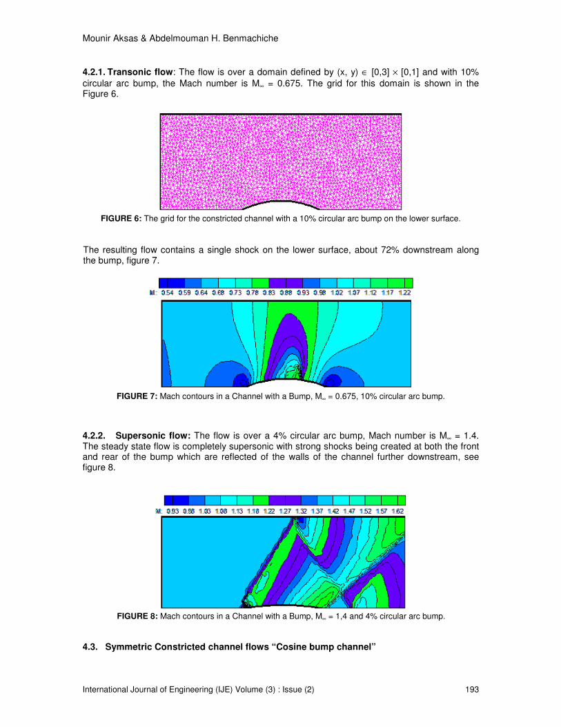
Mounir Aksas & Abdelmouman H. Benmachiche
International Journal of Engineering (IJE) Volume (3) : Issue (2) 193
4.2.1. Transonic flow: The flow is over a domain defined by (x, y) ∈ [0,3] × [0,1] and with 10%
circular arc bump, the Mach number is M∞ = 0.675. The grid for this domain is shown in the Figure 6.
FIGURE 6: The grid for the constricted channel with a 10% circular arc bump on the lower surface.
The resulting flow contains a single shock on the lower surface, about 72% downstream along the bump, figure 7.
FIGURE 7: Mach contours in a Channel with a Bump, M∞ = 0.675, 10% circular arc bump.
4.2.2. Supersonic flow: The flow is over a 4% circular arc bump, Mach number is M∞ = 1.4. The steady state flow is completely supersonic with strong shocks being created at both the front and rear of the bump which are reflected of the walls of the channel further downstream, see figure 8.
FIGURE 8: Mach contours in a Channel with a Bump, M∞ = 1,4 and 4% circular arc bump.
4.3. Symmetric Constricted channel flows “Cosine bump channel”

Mounir Aksas & Abdelmouman H. Benmachiche
International Journal of Engineering (IJE) Volume (3) : Issue (2) 194
In the third test case the computational domain represents a channel of length 3 meters and width 1 meter, with bumps of the same shape and size in the centre of either wall of the channel. The bumps are one meter in length and are defined such that the breadth of the channel is given by:
20 2 c
h
l
x xB B B cos
xπ
−= − ⋅
for
2
lc
xx x ,− ≤ (29)
Where: B0 =1 is the breadth of the channel. Bh is the height of each bump, in this case is taken to be 0.04. xc=1.5 is the x coordinate of the center of the constriction. Xl =1 is the length of each bump. The grid, shown in Figure 9 contains 2631 nodes and 5050 triangular cells.
FIGURE 9: The grid for the symmetric constricted channel flow test cases.
4.3.1. Subsonic case:
The inflow Mach number is given as M∞ = 0,5, the resulting steady solution is a subsonic, isentropic, symmetric solution about the bump, see figure 10. The boundary conditions are: the upper and lower surfaces are solid walls, and characteristic conditions are applied at the subsonic inlet and outlet.
FIGURE 10: The grid for the symmetric constricted channel flow test cases.
4.3.2. Transonic case:
In this case we consider Mach number is M∞ = 0.71. We remark the appearance of a band of shock downstream from the two arcs which gives a normal shock wave, see figure 11.
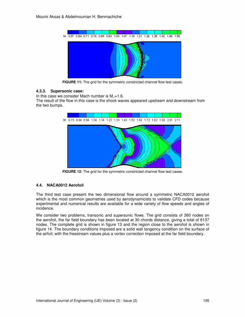
Mounir Aksas & Abdelmouman H. Benmachiche
International Journal of Engineering (IJE) Volume (3) : Issue (2) 195
FIGURE 11: The grid for the symmetric constricted channel flow test cases.
4.3.3. Supersonic case:
In this case we consider Mach number is M∞=1.6. The result of the flow in this case is the shock waves appeared upstream and downstream from the two bumps.
FIGURE 12: The grid for the symmetric constricted channel flow test cases.
4.4. NACA0012 Aerofoil The third test case present the two dimensional flow around a symmetric NACA0012 aerofoil which is the most common geometries used by aerodynamicists to validate CFD codes because experimental and numerical results are available for a wide variety of flow speeds and angles of incidence.
We consider two problems, transonic and supersonic flows. The grid consists of 260 nodes on the aerofoil, the far field boundary has been located at 30 chords distance, giving a total of 6137 nodes. The complete grid is shown in figure 13 and the region close to the aerofoil is shown in figure 14. The boundary conditions imposed are a solid wall tangency condition on the surface of the airfoil; with the freestream values plus a vortex correction imposed at the far field boundary.
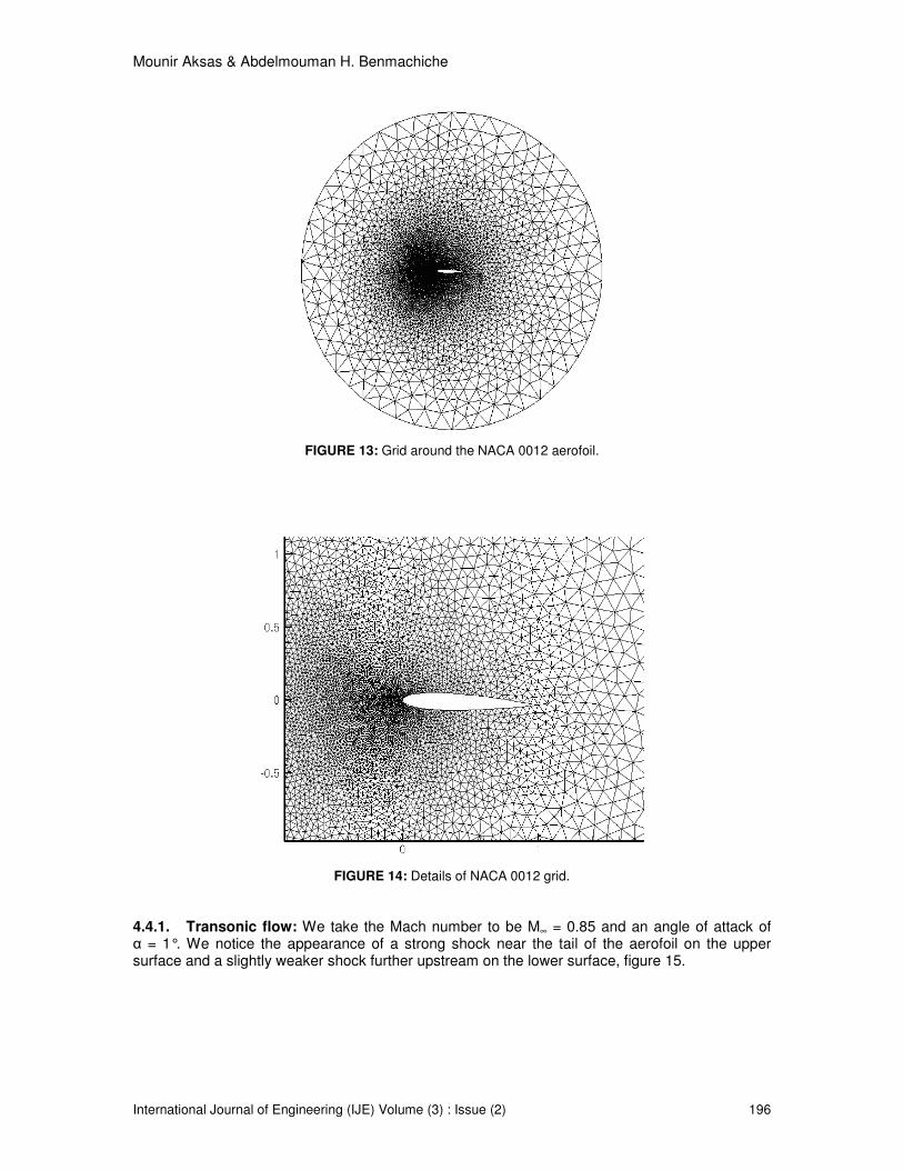
Mounir Aksas & Abdelmouman H. Benmachiche
International Journal of Engineering (IJE) Volume (3) : Issue (2) 196
FIGURE 13: Grid around the NACA 0012 aerofoil.
FIGURE 14: Details of NACA 0012 grid.
4.4.1. Transonic flow: We take the Mach number to be M∞ = 0.85 and an angle of attack of α = 1°. We notice the appearance of a strong shock near the tail of the aerofoil on the upper surface and a slightly weaker shock further upstream on the lower surface, figure 15.
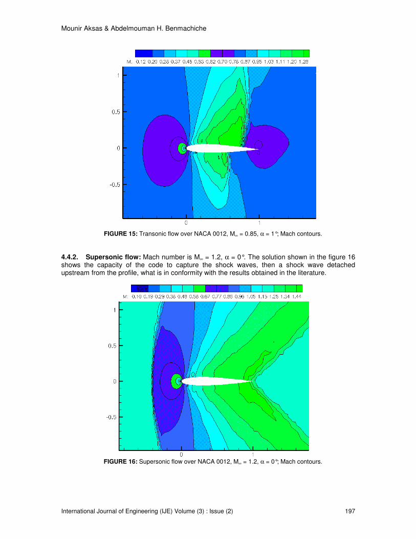
Mounir Aksas & Abdelmouman H. Benmachiche
International Journal of Engineering (IJE) Volume (3) : Issue (2) 197
FIGURE 15: Transonic flow over NACA 0012, M∞ = 0.85, α = 1°; Mach contours.
4.4.2. Supersonic flow: Mach number is M∞ = 1.2, α = 0°. The solution shown in the figure 16 shows the capacity of the code to capture the shock waves, then a shock wave detached upstream from the profile, what is in conformity with the results obtained in the literature.
FIGURE 16: Supersonic flow over NACA 0012, M∞ = 1.2, α = 0°; Mach contours.
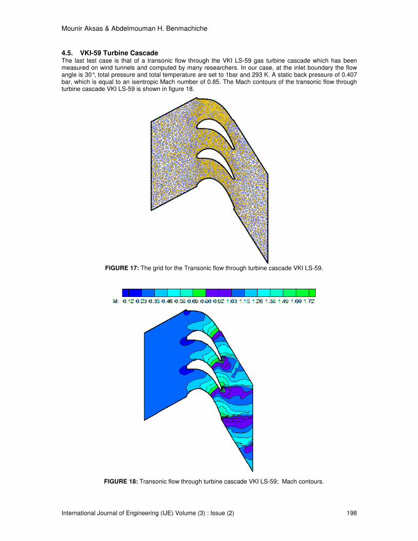
Mounir Aksas & Abdelmouman H. Benmachiche
International Journal of Engineering (IJE) Volume (3) : Issue (2) 198
4.5. VKI-59 Turbine Cascade The last test case is that of a transonic flow through the VKI LS-59 gas turbine cascade which has been measured on wind tunnels and computed by many researchers. In our case, at the inlet boundary the flow angle is 30°, total pressure and total temperature are set to 1bar and 293 K. A static back pressure of 0.407 bar, which is equal to an isentropic Mach number of 0.85. The Mach contours of the transonic flow through turbine cascade VKI LS-59 is shown in figure 18.
FIGURE 17: The grid for the Transonic flow through turbine cascade VKI LS-59.
FIGURE 18: Transonic flow through turbine cascade VKI LS-59; Mach contours.

Mounir Aksas & Abdelmouman H. Benmachiche
International Journal of Engineering (IJE) Volume (3) : Issue (2) 199
5. CONCLUSION & FUTURE WORK
The aim of this work is achieved, for each of the test cases the original Roe wave model type D is applied (which decompose the Euler equations into a set of six simple wave equations). When this model is combined with the fluctuation splitting N scheme it gives a very robust method for solving the Euler equations in complex geometries.
The purpose of the numerical results reported in our work show that our code written in C++ is comparable in accuracy, efficiency and robustness to others.
The ability of the code to capture the shock waves in different regimes: subsonic, transonic and supersonic flows has been illustrated, our results in all test cases are comparable with those produced in the literature.
In the future, we intend to study the efficiency of multidimensional upwind methods for the solution of conservation laws by applying grid adaptation (Effect of mesh refinement and the movement of nodes).
Acknowledgments
The authors would like to thank members of the “Laboratory Jacques-Louis Lions, University of Pierre et Marie Curie” in Paris, who provided the authors with the software Emc2: is a portable, interactive and graphic software Edition of two dimensional geometry and mesh generator.
REFERENCES
1. PL. Roe. “Approximate Riemann solvers, parameter vectors and difference schemes”. J. Computational Physics. 43(2):357-372, 1981.
2. H. Deconinck, R. Struijs, G. Bourgois, PL. Roe. “High resolution shock capturing cell vertex
advection schemes for unstructured grids”. Lecture series, Van Kareman Institute for
fluid dynamics. 5: H1-H79,1994.
3. H. Deconinck, R. Struijs, G. Bourgois, H. Paillere, PL. Roe. “Multidimensional upwind methods for unstructured grids. In AGARD, Special Course on Unstructured Grid Methods for Advection Dominated Flows. N92-27671 18-34, 1992.
4. H. Deconinck, PL., Roe, R. Struijs. “A multidimensional generalization of roe’s flux difference splitter for the Euler equations”. Journal of Computers Fluids. 22:215-222, 1993.
5. R. Struijs, H. Deconinck, P. De Palma, PL. Roe, KG. Powell. “Progress on multidimensional upwind Euler solvers for unstructured grids”. In Computational Fluid Dynamics Conference, 10th, Honolulu, HI, June 24-26, 1991.
6. H. Paillere, H. Deconinck, E. Van der Weide. “Upwind residual distribution methods for compressible flow”. In 28th CFD Lecture Series, Bruxelles, VKI for Fluid Dynamics, 1997.

Mounir Aksas & Abdelmouman H. Benmachiche
International Journal of Engineering (IJE) Volume (3) : Issue (2) 200
7. PL. Roe. “Discrete models for the numerical analysis of time-dependent multidimensional gas dynamics”. Journal of Computational Physics, 43:458-476, 1986.
8. PL. Roe. “Algorithmic trends in CFD, chapter Beyond the Riemann Problem”. Springer-Verlag, Part I, 341-367, 1993.
9. D. Sidilkover, PL. Roe. “Unifaction of some advection schemes in two dimensions”. Technical report, ICASE, TR-95-10, 1995.
10. ME. Hubbard. “Multidimensional Upwinding and grid adaptation for conservation Laws”. PhD Thesis, University of Reading, 1996.
11. L. Mesaros. “Multi-Dimensional Fluctuation Schemes for the Euler Equations on Unstructured Grids”. PhD Thesis, University of Michigan,1995.
12. N. Venkatakrishnan. “A Perspective on Unstructured Grid Flow Solvers”. ICASE Report 95-3, 1995.
13. PL. Roe, L. Mesaros. “An improved wave model for the multi-dimensional upwinding of the Euler equations”. In Proceedings of the Thirteenth International Conference on Numerical Methods in Fluid Dynamics, Rome, July 1992.
14. P. De Palma, H. Deconinck and R. Struijs. “Investigation of Roe’s 2D wave decomposition models for the Euler equations”. Technical report, Von Karman Institute for Fluid Dynamics, TN-172, June 1990.
15 B. Laskarzewska and M. Mehrvar. “Atmospheric Chemistry in Existing Air Atmospheric Dispersion Models and Their Applications: Trends, Advances and Future in Urban Areas in Ontario, Canada and in Other Areas of the World”. International Journal of Engineering (IJE),
Volume (3) : Issue (1), 2009.
16 R. Atan, A. A. A. Ghani, M. Selamat and R. Mahmod.“Automating Measurement for Software Process Models using Attribute Grammar Rules”. International Journal of Engineering (IJE),
Volume (1) : Issue (2), 2007.
17 S. Manchanda, M. Dave and S. B. Singh. “Genetic Information System Development and Maintenance Model For Effective Software Maintenance and Reuse”. International Journal of Engineering (IJE), Volume (1) : Issue (1), 2007.

Deepika Garg, Kuldeep Kumar & Jai Singh
International Journal of Engineering (IJE), Volume (3) : Issue (2) 201
Availability Analysis of A Cattle Feed Plant Using Matrix Method
Deepika Garg [email protected] Research scholar, Dept of Mathematics N.I.T., Kurukshetra, India
Kuldeep Kumar [email protected] Prof. and Chairman, Dept of Mathematics, N.I.T., Kurukshetra, India
Jai Singh [email protected] Principal, M.I.E.T, Mohri, Kurukshetra, India
ABSTRACT
A matrix method is used to estimate the probabilities of complex system events by simple matrix calculation. Unlike existing methods, whose complexity depends highly on the system events, the matrix method describes the general system event in a simple matrix form. Therefore, the method provides an easy way to estimate the variation in system performance in terms of availability with respect to time.
Purpose- The purpose of paper is to compute availability of cattle feed plant .A Cattle feed plant consists of seven sub-systems working in series. Two subsystems namely mixer and palletiser are supported by stand-by units having perfect switch over devices and remaining five subsystems are subjected to major failure.
Methodology/approach- The mathematical model of Cattle feed plant has been developed using Markov birth – death Process.The differential equations are solved using matrix method and a C-program is developed to study the variation of availability with respect to time.
Findings- The study of analysis of availability can help in increasing the production and quality of cattle feed. To ensure the system performance throughout its service life, it is necessary to set up proper maintenance planning and control which can be done after studying the variation of availability with respect to time.
Originality/value- Industrial implications of the results have been discussed.
Keywords: Availability, Differential Equations, Markov Process, Matrix Method.

Deepika Garg, Kuldeep Kumar & Jai Singh
International Journal of Engineering (IJE), Volume (3) : Issue (2) 202
1 INTRODUCTION
Modern engineering systems like process and energy systems, transport systems, offshore structures, bridges, pipelines are design to ensure the successful operation throughout the anticipated service life. Unfortunately there is a threat of deterioration of processes, so it is necessary to study the variation of availability with respect to time. The objective of the present paper is to analysis the availability of cattle feed plant. Cattle feed plant mainly consists of seven subsystems namely Elevator, Grinder, Hopper, Mixer, Winch, Palletiser and Screw conveyor. These units are arranged in series. Failure and repair rates of each machine are assumed to be constant. The mathematical model of cattle feed plant has been developed using Markov birth – death Process. The differential equations have been developed on the basis of probabilistic approach using transition diagram. Matrix method is used to solve these equations and calculations are done with the help of c-program. Won-Hee Kang, Junho Song and Paolo Gardoni [18] discussed the matrix based system to calculate system reliability. The findings of the present paper can be considered to be useful for the analysis of availability and for determining the best possible maintenance strategies for a cattle feed plant concerned.
2. LITERATURE SURVEY
The last decades has witnessed a growing interest in the development and application of reliability methods in the field of various industrial sectors related with maintenance engineering and management. Recently, many researchers have discussed reliability of different process industries using different techniques. Kumar and Singh [2] analyzed the Availability of a washing system of paper industry. Singh, Kumar and Pandey [3, 5] discussed the reliability and availability of Fertilizer and Sugar industry .Dayal and singh [4] studied reliability analysis of a system in a fluctuating environment. Zaho [6] developed a generalized availability model for repairable component and series system including perfect and imperfect repair. Michelson [7] discussed the use of reliability technology in process industry. Singh and Mahajan [8] examined the reliability and long run availability of a Utensils Manufacturing Plant using Laplace transforms. Günes and Deveci [9] have studied the reliability of service systems and its application in student office and Habchi [10] discussed and improved the method of reliability assessment for suspended test . Jain [11] discussed N-Policy for redundant repairable system with additional repairman. Gupta, Lal, Sharma and Singh [12] discussed the reliability, long term availability and MTBF of cement industry with the help of Runga – Kutta method. Kiureghian and Ditlevson [13] analyzed the availability, reliability & downtime of system with repairable components. Kumar, Singh and Sharma [15] discussed the availability of an automobile system namely “scooty”. Tewari, Kumar, Kajal and Khanduja [16] discussed the availability of a Crystallization unit of a sugar plant. In these papers, authors used either Laplace transforms method or Lagrange’s or runge-kutta method to solve differential associated with particular problem. Jussi K.Vaurio [17] discussed current research and application related to the modeling, optimization and application of maintenance procedures for ageing and deteriorating engineering and structural systems. It has been observed that these methods involve complex computations and it is very difficult to calculate availability/reliability of the system by these methods. In fact, problem of calculating variation of availability with time has not satisfactorily been tackled till now. This leads to the development of matrix method in order to calculate reliability of the system. In the present paper, matrix method is used and then computer program is developed to calculate the value of availability at various interval of time. The variation in the availability of cattle feed plant is also shown with the help of graph.
3. THE SYSTEM
The Cattle feed plant mainly consists of seven subsystems namely Elevator, Grinder, Hopper, Mixer, Winch, Palletiser, Screw conveyor. Initially Elevator lifts the material and put it into the Grinder. Grinder grinds the raw material and then the material is put into the Hopper. Hopper is used for the storage and cooling of material. Cooling is done by the fans present in the Hopper. Then the material is put into the Mixer for proper mixing of certain additives in specified ratio. This mixture is lift by Winch which put this mixture into the Palletiser. Palletiser allows the mixture to move forward and passes through holes which give them a proper shape. Finally Screw conveyor carries the final product to the store where it is packed for final delivery

Deepika Garg, Kuldeep Kumar & Jai Singh
International Journal of Engineering (IJE), Volume (3) : Issue (2) 203
The Cattle feed plant consists of the following seven main subsystems: I. Elevator (A) consists of one unit. The system fails when this subsystem fails.
II. Grinder (B) consists of one unit. It is subjected to major failure only. III. Hopper (C) consists of one unit. It is subjected to major failure only. IV. Mixer (D) consists of two units, one working and the other is in cold standby. The cold standby unit is of
lower capacity. The system works on standby unit in reduced capacity. Complete failure occurs when both units fail.
V. Winch (E) consists of one unit. The system fails when this subsystem fails VI. Palletiser (F) consists of two units, one working and the other is in cold standby. The cold standby unit is of
lower capacity. The system works on standby unit in reduced capacity. Complete failure occurs when both units fail.
VII. Screw conveyor (G) consists of one unit. The system fails when this subsystem fails
4. ASSUMPTIONS AND NOTATIONS I. Repair rates and failure rates are negative exponential and independent of each other. II. Not more than one failure occurs at a time. III. A repaired unit is, performance wise, as good as new. IV. The subsystems D and F fail through reduced states. V. Switch-over devices are perfect.
A, B, C, D, E, F, G : Capital letters are used for good states. D , F : Denotes the reduced capacity states. a, b, c, d, e, f, g : Denotes the respective failed states.
λ i : Indicates the respective mean failure rates of Elevator, Grinder, Hopper, Mixer, Winch, Palletiser, Screw conveyor. i =1,2,3,4,5,6,7,8,9. i = 5 and 8 stands for failure rates of reduced states of D and F respectively.
µi : Indicates the respective repair rates of Elevator, Grinder, Hopper , Mixer,
Winch, Palletiser, Screw conveyor, i =1,2,3,4,5,6,7,8,9. i = 5 and 8 stands for repair rates of reduced states of D and F respectively.
Pi (t) : Probability that the system is in i th state at time t.
Pi ' (t) : Derivative of probability function Pi (t).
5. MATHEMATICAL MODELING Probabilistic considerations give the following differential equations, associated with the transition diagram as given by figure 2.
1 1 1 1 5 2 6 3 7 6 8 9 9 4 4 7 2'( ) ( ) ( ) ( ) ( ) ( ) ( ) ( ) ( )p t a p t p t p t p t p t p t p t p tµ µ µ µ µ µ µ= + + + + + + +
2 2 2 1 21 2 20 3 19 4 3 6 18 8 17 9 16 7 1'( ) ( ) ( ) ( ) ( ) ( ) ( ) ( ) ( ) ( )p t a p t p t p t p t p t p t p t p t p tµ µ µ µ µ µ µ λ= + + + + + + + +
3 3 3 1 28 2 27 3 26 5 25 6 24 8 23 9 22 4 2 7 4'( ) ( ) ( ) ( ) ( ) ( ) ( ) ( ) ( ) ( ) ( )p t a p t p t p t p t p t p t p t p t p t p tµ µ µ µ µ µ µ λ λ= + + + + + + + + +
4 4 4 1 15 2 14 3 13 5 12 6 11 9 10 7 3 4 1'( ) ( ) ( ) ( ) ( ) ( ) ( ) ( ) ( ) ( )p t a p t p t p t p t p t p t p t p t p tµ µ µ µ µ µ µ λ= + + + + + + + +
Where
1 1 2 3 6 9 4 7( )a λ λ λ λ λ λ λ= − + + + + + +
2 1 2 3 4 6 8 9 7( )a λ λ λ λ λ λ λ µ= − + + + + + + +
3 1 2 3 5 6 8 9 4 7( )a λ λ λ λ λ λ λ µ µ= − + + + + + + + +
4 1 2 3 5 6 7 9 4( )a λ λ λ λ λ λ λ µ= − + + + + + + +
1'( ) ( ) ( )
5,6,7,8,9; 1, 2,3,6,9;
i j i jp t p t p t
i j
µ λ+ =
= =

Deepika Garg, Kuldeep Kumar & Jai Singh
International Journal of Engineering (IJE), Volume (3) : Issue (2) 204
2'( ) ( ) ( )
16,17,18,19,20,21; 9,8,6,3, 2,1;
i j i jp t p t p t
i j
µ λ+ =
= =
3'( ) ( ) ( )
22,23, 24, 25,26,27, 28; 9,8,6,5,3,2,1;
i j i jp t p t p t
i j
µ λ+ =
= =
4'( ) ( ) ( )
10,11,12,13,14,15; 9,6,5,3, 2,1;
i j i jp t p t p t
i j
µ λ+ =
= =
With initial conditions P1 (0) =1, otherwise zero.
Let p(k, t) denotes the transition probability of the event that the system is in state k at the time t. Since the number of all the possible transition states of the complex system is‘28’.So the system of differential difference equations for above equations may be written as;
(θI-A) P (k, t) = 0
Where θ = d/dt, 0 is the null matrix, matrix A is the matrix of coefficients of Pi (t)’s in differential difference equation
Matrix A=

Deepika Garg, Kuldeep Kumar & Jai Singh
International Journal of Engineering (IJE), Volume (3) : Issue (2) 205
1 7 4 1 2 3 6 9
7 2 4 9 8 6 3 2 1
4 3 7 9 8 6 5 3 2 1
4 7 4 9 6 5 3 2 1
1 1
2 2
0 0 0 0 0 0 0 0 0 0 0 0 0 0 0 0 0 0 0 0
0 0 0 0 0 0 0 0 0 0 0 0 0 0 0 0 0 0 0
0 0 0 0 0 0 0 0 0 0 0 0 0 0 0 0 0 0
0 0 0 0 0 0 0 0 0 0 0 0 0 0 0 0 0 0 0
0 0 0 0 0 0 0 0 0 0 0 0 0 0 0 0 0 0 0 0 0 0 0 0 0 0
0 0 0 0 0 0 0 0 0 0 0 0
a
a
a
a
µ µ µ µ µ µ µ
λ µ µ µ µ µ µ µ
λ λ µ µ µ µ µ µ µ
λ µ µ µ µ µ µ µ
λ µ
λ µ
−
−
−
−
−
−
3 3
6 6
9 9
9 9
6 6
5 5
0 0 0 0 0 0 0 0 0 0 0 0 0 0
0 0 0 0 0 0 0 0 0 0 0 0 0 0 0 0 0 0 0 0 0 0 0 0 0 0
0 0 0 0 0 0 0 0 0 0 0 0 0 0 0 0 0 0 0 0 0 0 0 0 0 0
0 0 0 0 0 0 0 0 0 0 0 0 0 0 0 0 0 0 0 0 0 0 0 0 0 0
0 0 0 0 0 0 0 0 0 0 0 0 0 0 0 0 0 0 0 0 0 0 0 0 0 0
0 0 0 0 0 0 0 0 0 0 0 0 0 0 0 0 0 0 0 0 0 0 0 0 0 0
0 0 0 0 0 0 0 0 0 0 0 0 0 0 0 0 0 0 0 0 0 0 0 0 0 0
λ µ
λ µ
λ µ
λ µ
λ µ
λ µ
−
−
−
−
−
−
3 3
2 2
1 1
9 9
8 8
6 6
3
0 0 0 0 0 0 0 0 0 0 0 0 0 0 0 0 0 0 0 0 0 0 0 0 0 0
0 0 0 0 0 0 0 0 0 0 0 0 0 0 0 0 0 0 0 0 0 0 0 0 0 0
0 0 0 0 0 0 0 0 0 0 0 0 0 0 0 0 0 0 0 0 0 0 0 0 0 0
0 0 0 0 0 0 0 0 0 0 0 0 0 0 0 0 0 0 0 0 0 0 0 0 0 0
0 0 0 0 0 0 0 0 0 0 0 0 0 0 0 0 0 0 0 0 0 0 0 0 0 0
0 0 0 0 0 0 0 0 0 0 0 0 0 0 0 0 0 0 0 0 0 0 0 0 0 0
0 0 0 0 0 0 0 0 0 0 0 0
λ µ
λ µ
λ µ
λ µ
λ µ
λ µ
λ
−
−
−
−
−
−
3
2 2
1 1
9 9
8 8
6 6
5 5
0 0 0 0 0 0 0 0 0 0 0 0 0 0
0 0 0 0 0 0 0 0 0 0 0 0 0 0 0 0 0 0 0 0 0 0 0 0 0 0
0 0 0 0 0 0 0 0 0 0 0 0 0 0 0 0 0 0 0 0 0 0 0 0 0 0
0 0 0 0 0 0 0 0 0 0 0 0 0 0 0 0 0 0 0 0 0 0 0 0 0 0
0 0 0 0 0 0 0 0 0 0 0 0 0 0 0 0 0 0 0 0 0 0 0 0 0 0
0 0 0 0 0 0 0 0 0 0 0 0 0 0 0 0 0 0 0 0 0 0 0 0 0 0
0 0 0 0 0 0 0 0 0 0 0 0 0 0 0 0 0 0 0 0 0 0 0
µ
λ µ
λ µ
λ µ
λ µ
λ µ
λ µ
−
−
−
−
−
−
−
3 3
2 2
1 1
0 0 0
0 0 0 0 0 0 0 0 0 0 0 0 0 0 0 0 0 0 0 0 0 0 0 0 0 0
0 0 0 0 0 0 0 0 0 0 0 0 0 0 0 0 0 0 0 0 0 0 0 0 0 0
0 0 0 0 0 0 0 0 0 0 0 0 0 0 0 0 0 0 0 0 0 0 0 0 0 0
λ µ
λ µ
λ µ
−
− −

Deepika Garg, Kuldeep Kumar & Jai Singh
International Journal of Engineering (IJE), Volume (3) : Issue (2) 206
P (k, t) = [P1(t) P2(t) ………………………………P28(t)]T and I 28x28 is the identity matrix. Let C be the matrix such that C
-1 AC = D Where D = (d1, d2, ……..d28) be the diagonal matrix of Eigen values of
the matrix A. We may write C
-1 (θ1-A) P (k, t) = 0 gives
(θ1-D) G (k, t) = 0 where G (k, t) = C
-1 P (k,t)
Equation is a matrix linear differential equation in G(k, t) having solution G (k, t) e
-Dt = K, for some constant K, with initial conditions P1(0) = 1 and 0 otherwise,
We get, K = C
-1 P (k, 0), where P (k, 0) = [1 0 0 0 0………0]
T .
G (k, t) = e
Dt C
-1 P (k, 0) gives,
P (k, t) = C(1+ Dt + D
2t2 /2! + ……….) C
-1 P (k, 0)
= P (k, 0) + A P (k,0) t + A
2 P (k,0) t
2 / 2! + ………………..
= P (k, 0) + L1t + L2 t
2 /2! + ………Ln t
n / n! +………… where Ln = A
n P (k, 0) and
P (k, 0) is the column matrix of order 28 x 1 The initial conditions make it clear that P (k, 0) is the column matrix (1 0 0 0 ……0)
T ,
A P (k, 0) is just the 1
st column of the matrix A. let us denote this column matrix by
A1 = (a11, a12, …….. a1,28)
T.
A
2 P (k, 0) = AA P (k, 0) = AA1 is again a column matrix, let us denote it by
A2 = (b11, b12, ………, b1, 28)
T.
Let A
r-1 P (k, 0) = A r-1 = ( P11 ,P12,………….,P 1,28)
T
The examination reveals that A
r P (k, 0) = A A r-1 = (q11, q12 ,……..,q1,28)
T, say
Transition state availability of different stages are; P (1, t) = 1 + a11t + b11t
2 / 2! + …………..
P (2, t) = a21t + b21t
2 / 2! + ………………
…………………………………………… ……………………………………………
P (i, t) = ai1t + bi1 t
2 / 2! + ………………
Since P (1, t), P (2, t), P (3, t), P (4, t) are the only working states of a system, so
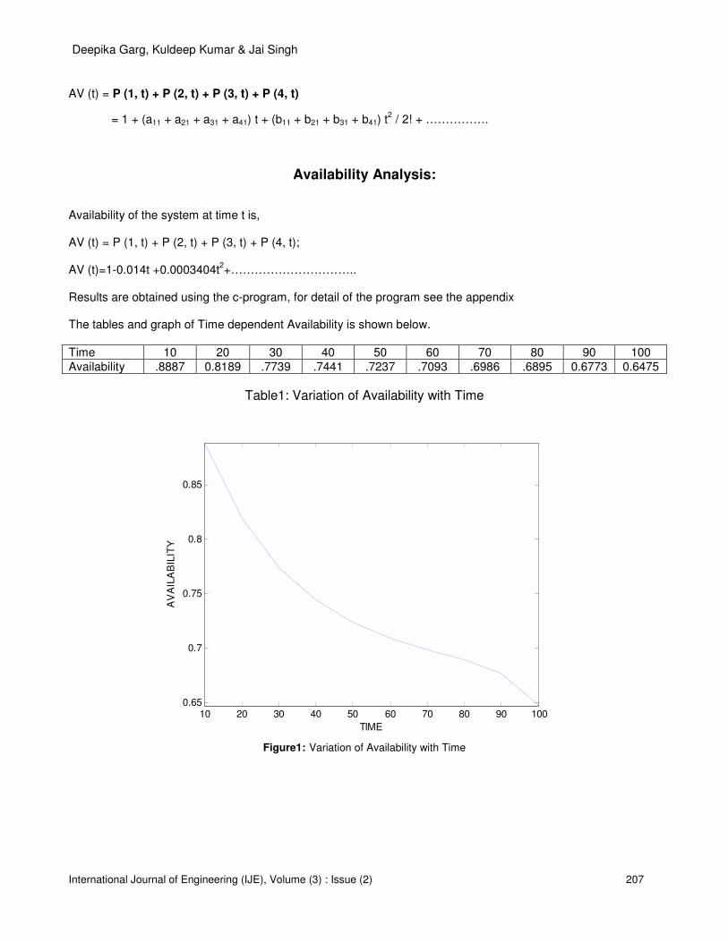
Deepika Garg, Kuldeep Kumar & Jai Singh
International Journal of Engineering (IJE), Volume (3) : Issue (2) 207
AV (t) = P (1, t) + P (2, t) + P (3, t) + P (4, t)
= 1 + (a11 + a21 + a31 + a41) t + (b11 + b21 + b31 + b41) t2 / 2! + …………….
Availability Analysis:
Availability of the system at time t is, AV (t) = P (1, t) + P (2, t) + P (3, t) + P (4, t); AV (t)=1-0.014t +0.0003404t
2+…………………………..
Results are obtained using the c-program, for detail of the program see the appendix The tables and graph of Time dependent Availability is shown below.
Time 10 20 30 40 50 60 70 80 90 100
Availability .8887 0.8189 .7739 .7441 .7237 .7093 .6986 .6895 0.6773 0.6475
Table1: Variation of Availability with Time
10 20 30 40 50 60 70 80 90 1000.65
0.7
0.75
0.8
0.85
TIME
AV
AIL
AB
ILIT
Y
Figure1: Variation of Availability with Time

Deepika Garg, Kuldeep Kumar & Jai Singh
International Journal of Engineering (IJE), Volume (3) : Issue (2) 208
6. CONCLUSIONS & FUTURE WORK
The present paper can help in increasing the production and quality of cattle feed. The proposed method can be applied to complex systems that include a large system of differential equations. Using this method, we can easily study the variation of availability with respect to time. The differential equations are solved using Matrix method and a C-program is used to calculate availability of cattle feed plant. Table 1 and figure 1 shows the variation of availability with respect to time. Initially availability decreases sharply with respect to time and become almost stable after long duration of time. The same methodology can be applied in other industries so
that the management can get maximum benefit from the same.
7. REFERENCES [1] B.S. Dhillon, and C.Singh, “Engineering Reliability New Techniques and Applications”, John Wiley and
sons. , 1981 [2] D.Kumar, and J.Singh, “Availability of a Washing System in the Paper Industry”, Microelectron. Reliability,
Vol. 29, pp.775-778, 1989 [3] J.Singh, P.C.Pandey and D.Kumar, “Designing for Reliable Operation of Urea Synthesis in the Fertilizer
Industry”, Microelectron. Reliability, Vol. 30, pp.1021-1024., 1990 [4] B.Dayal and J.Singh, “Reliability analysis of a system in a fluctuating envioronment”, Microelectron
Reliability, Vol.32, pp.601-603, 1992. [5] D.Kumar, J.Singh, and P.C.Pandey “Availability of the Crystallization System in the Sugar Industry
under Common – Cause Failure”, IEEE Transactions on Reliability, Vol. 41, No.1, pp 85-91., 1992 [6] M.Zhao, “Availability for Repairable components and series systems”, IEEE Transactions on Reliability, Vol-43, No.2, 1994 [7] Q. Michelson, “Use of Reliability Technology in The Process Industry”, Reliability
Engineering and system safety, 60, pp.179-181, 1998 [8] J.Singh, and P Mahajan, “Reliability of Utensils Manufacturing Plant – A Case Study”, Opsearch, Vol. 36,
No.3, pp 260-269., 1999. [9] McGuiness and I. Deveci, “Reliability of service system and an application in student office”, International
Journal of Quality & Reliability Management, Vol.19, pp.206-211, 2002 [10] G. Habchi, “An improved method of reliability assessment for suspended tests”, International Journal of
Quality & Reliability Management, vol.19, pp.454-470, 2002 [11] Madhu Jain, “N-Policy for redundant repairable system with additional repairmen”, Opsearch, vol 4, 97-114,
2003 [12] P Gupta., A.K.Lal, R.K.Sharma and J.Singh “Behavioral Study of the Cement manufacturing Plant – A
Numerical Approach” , Journal of Mathematics and Systems Sciences, Vol. 1, No. 1,pp.50-69.,2005 [13] A.D.Kiureghian and O.D.Ditlevson, “Availability, Reliability & downtime of system with repairable
components”, Reliability Engineering and System Safety, Volume 92, Issue 2, pp. 66-72.,2007 [14] Jai Singh Gurjar, “Reliability Technology – Theory and Applications”; I.K. International Publishing House
Pvt. Ltd. New Delhi (I ndia). 2007 [15] J.Singh, K Kumar, A.Sharma, “Availability Evaluation of an Automobile System”, Journal of mathematics
and system sciences, Vol. 4, No.2, pp.95-102., 2008

Deepika Garg, Kuldeep Kumar & Jai Singh
International Journal of Engineering (IJE), Volume (3) : Issue (2) 209
[16] P.C Tewari, D.Kumar, S.Kajal, R.Khanduja,"Decision support system for the Crystallization unit of a sugar plant", Icfai J. of Science and Technology, Vol-4, No.3, pp.7-16, 2008 [17] Enrio Zio and Jussi K.Vaurio “Maitenance modeling and applications”, Reliability Engineering and System
safety, vol-94, Issue 1, Page 1. [18] Won-Hee Kang,Junho Song and Paolo Gardoni , “Matrix –based system reliability method
applications to bridge networks”,” Reliability Engineering and System Safety”,vol-93,issue 11,pp.1584- 1593
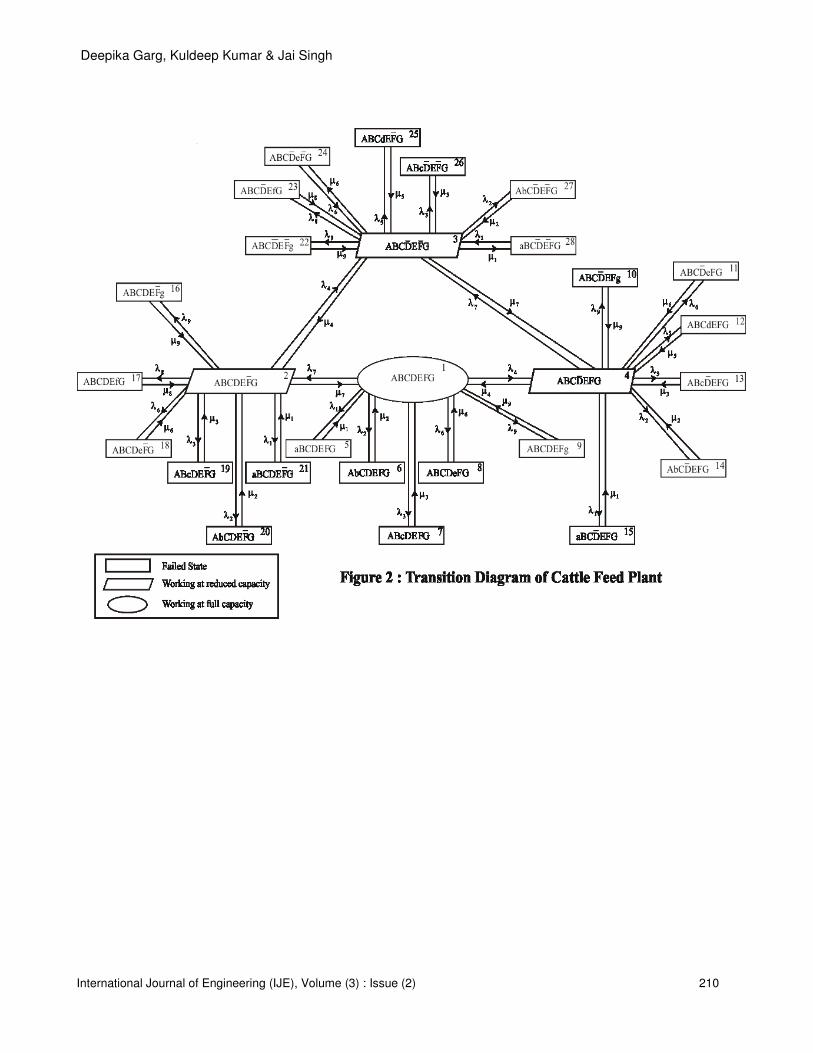
Deepika Garg, Kuldeep Kumar & Jai Singh
International Journal of Engineering (IJE), Volume (3) : Issue (2) 210

Deepika Garg, Kuldeep Kumar & Jai Singh
International Journal of Engineering (IJE), Volume (3) : Issue (2) 211
APPENDIX
#include<stdio.h>
#include<conio.h>
void main()
{
float a[28][28],b[28][28],c[28][28],d[28][28];
float e[28][28],f[28][28],g[28][28],h[28][28];
float p[28][28],q[28][28],r[28][28],s[28][28];
float u[28][28],v[28][28];
float x1,x2,x3,x4,x5,x6,x7,x8,x9,y1,y2,y3,y4,y5,y6,y7,y8,y9;
int t;
float a1,a2,a3,a4;
float av1,av2,av3,av4,av5,av6,av7,av8,av9,av10,av11,av12,av13,av;
int i,j,k,m=28,n=28;
x1=.002;
x2=.001;
x3=.004;
x4=.0025;
x5=.0025;
x6=.005;
x7=.003;
x8=.003;
x9=.002;
y1=.02;
y2=.01;
y3=.04;
y4=.02;
y5=.02;

Deepika Garg, Kuldeep Kumar & Jai Singh
International Journal of Engineering (IJE), Volume (3) : Issue (2) 212
y6=.05;
y7=.03;
y8=.03;
y9=.02;
printf("\n\n\n");
printf("\n at what time u want to find reliability t=");
scanf("%d",&t);
for(i=0;i<m;i++)
{
for(j=0;j<n;j++)
{
a[i][j]=0;
}
}
a1=-(x1+x2+x3+x4+x6+x9+x7);
a[0][0]=a1;
a[0][1]=y7;
a[0][3]=y4;
a[0][4]=y1;
a[0][5]=y2;
a[0][6]=y3;
a[0][7]=y6;
a[0][8]=y9;
a[1][0]=x7;
a2=-(x1+x2+x3+x4+x6+x8+x9+y7);
a[1][1]=a2;
a[1][2]=y4;
a[1][15]=y9;
a[1][16]=y8;
a[1][17]=y6;

Deepika Garg, Kuldeep Kumar & Jai Singh
International Journal of Engineering (IJE), Volume (3) : Issue (2) 213
a[1][18]=y3;
a[1][19]=y2;
a[1][20]=y1;
a[2][1]=x4;
a3=-(x1+x2+x3+x5+x6+x8+x9+y4+y7);
a[2][2]=a3;
a[2][3]=x7;
a[2][21]=y9;
a[2][22]=y8;
a[2][23]=y6;
a[2][24]=y5;
a[2][25]=y3;
a[2][26]=y2;
a[2][27]=y1;
a[3][0]=x4;
a[3][2]=y7;
a4=-(x1+x2+x3+x5+x6+x7+x9+y4);
a[3][3]=a4;
a[3][9]=y9;
a[3][10]=y6;
a[3][11]=y5;
a[3][12]=y3;
a[3][13]=y2;
a[3][14]=y1;
a[4][0]=x1;
a[4][4]=-y1;
a[5][0]=x2;
a[5][5]=-y2;
a[6][0]=x3;
a[6][6]=-y3;

Deepika Garg, Kuldeep Kumar & Jai Singh
International Journal of Engineering (IJE), Volume (3) : Issue (2) 214
a[7][0]=x6;
a[7][7]=-y6;
a[8][0]=x9;
a[8][8]=-y9;
a[9][3]=x9;
a[9][9]=-y9;
a[10][3]=x6;
a[10][10]=-y6;
a[11][3]=x5;
a[11][11]=-y5;
a[12][3]=x3;
a[12][12]=-y3;
a[13][3]=x2;
a[13][13]=-y2;
a[14][3]=x1;
a[14][14]=-y1;
a[15][1]=x9;
a[15][15]=-y9;
a[16][1]=x8;
a[16][16]=-y8;
a[17][1]=x6;
a[17][17]=-y6;
a[18][1]=x3;
a[18][18]=-y3;
a[19][1]=x2;
a[19][19]=-y2;
a[20][1]=x1;
a[20][20]=-y1;
a[21][2]=x9;
a[21][21]=-y9;

Deepika Garg, Kuldeep Kumar & Jai Singh
International Journal of Engineering (IJE), Volume (3) : Issue (2) 215
a[22][2]=x8;
a[22][22]=-y8;
a[23][2]=x6;
a[23][23]=-y6;
a[24][2]=x5;
a[24][24]=-y5;
a[25][2]=x3;
a[25][25]=-y3;
a[26][2]=x2;
a[26][26]=-y2;
a[27][2]=x1;
a[27][27]=-y1;
for(i=0;i<m;i++)
{
for(j=0;j<n;j++)
{
b[i][j]=a[i][j];
}
}
for(i=0;i<m;i++)
{
j=0;
c[i][j]=0;
for(k=0;k<m;k++)
{
c[i][j]=c[i][j]+(a[i][k]*b[k][j]*t)/2;
}
}
for(i=0;i<m;i++)
{

Deepika Garg, Kuldeep Kumar & Jai Singh
International Journal of Engineering (IJE), Volume (3) : Issue (2) 216
j=0;
d[i][j]=0;
for(k=0;k<m;k++)
d[i][j]=d[i][j]+((a[i][k]*c[k][j]*t)/3);
}
for(i=0;i<m;i++)
{
j=0;
e[i][j]=0;
for(k=0;k<m;k++)
{
e[i][j]=e[i][j]+((a[i][k]*d[k][j]*t)/4);
}
}
for(i=0;i<m;i++)
{
j=0;
f[i][j]=0;
for(k=0;k<m;k++)
{
f[i][j]=f[i][j]+((a[i][k]*e[k][j]*t)/5);
}
}
for(i=0;i<m;i++)
{
j=0;
g[i][j]=0;
for(k=0;k<m;k++)
{
g[i][j]=g[i][j]+((a[i][k]*f[k][j]*t)/6);

Deepika Garg, Kuldeep Kumar & Jai Singh
International Journal of Engineering (IJE), Volume (3) : Issue (2) 217
}
}
for(i=0;i<m;i++)
{
j=0;
h[i][j]=0;
for(k=0;k<m;k++)
h[i][j]=h[i][j]+((a[i][k]*g[k][j]*t)/7);
}
for(i=0;i<m;i++)
{
j=0;
p[i][j]=0;
for(k=0;k<m;k++)
p[i][j]=p[i][j]+((a[i][k]*h[k][j]*t)/8);
}
for(i=0;i<m;i++)
{
j=0;
q[i][j]=0;
for(k=0;k<m;k++)
q[i][j]=q[i][j]+((a[i][k]*p[k][j]*t)/9);
}
for(i=0;i<m;i++)
{
j=0;
r[i][j]=0;
for(k=0;k<m;k++)
r[i][j]=r[i][j]+((a[i][k]*q[k][j]*t)/10);
}

Deepika Garg, Kuldeep Kumar & Jai Singh
International Journal of Engineering (IJE), Volume (3) : Issue (2) 218
for(i=0;i<m;i++)
{
j=0;
s[i][j]=0;
for(k=0;k<m;k++)
s[i][j]=s[i][j]+((a[i][k]*r[k][j]*t)/11);
}
for(i=0;i<m;i++)
{
j=0;
u[i][j]=0;
for(k=0;k<m;k++)
u[i][j]=u[i][j]+((a[i][k]*s[k][j]*t)/12);
}
for(i=0;i<m;i++)
{
j=0;
v[i][j]=0;
for(k=0;k<m;k++)
v[i][j]=v[i][j]+((a[i][k]*u[k][j]*t)/13);
}
av1=(a[0][0]+a[1][0]+a[2][0]+a[3][0])*t;
av2=(c[0][0]+c[1][0]+c[2][0]+c[3][0])*t;
av3=(d[0][0]+d[1][0]+d[2][0]+d[3][0])*t;
av4=(e[0][0]+e[1][0]+e[2][0]+e[3][0])*t;
av5=(f[0][0]+f[1][0]+f[2][0]+f[3][0])*t;
av6=(g[0][0]+g[1][0]+g[2][0]+g[3][0])*t;
av7=(h[0][0]+h[1][0]+h[2][0]+h[3][0])*t;
av8=(p[0][0]+p[1][0]+p[2][0]+p[3][0])*t;
av9=(q[0][0]+q[1][0]+q[2][0]+q[3][0])*t;

Deepika Garg, Kuldeep Kumar & Jai Singh
International Journal of Engineering (IJE), Volume (3) : Issue (2) 219
av10=(r[0][0]+r[1][0]+r[2][0]+r[3][0])*t;
av11=(s[0][0]+s[1][0]+s[2][0]+s[3][0])*t;
av12=(u[0][0]+u[1][0]+u[2][0]+u[3][0])*t;
av13=(v[0][0]+v[1][0]+v[2][0]+v[3][0])*t;
av=1+av1+av2+av3+av4+av5+av6+av7+av8+av9+av10+av11+av12+av13;
printf("\n availability of the system = %f",av);
getch();
}