INTERNATIONAL JOURNAL OF BIOMETRICS · 105 - 112 Novel Method to Quantify The Distribution of...
60
Transcript of INTERNATIONAL JOURNAL OF BIOMETRICS · 105 - 112 Novel Method to Quantify The Distribution of...


INTERNATIONAL JOURNAL OF BIOMETRICS AND BIOINFORMATICS (IJBB)
VOLUME 6, ISSUE 5, 2012
EDITED BY
DR. NABEEL TAHIR
ISSN (Online): 1985-2347
International Journal of Biometrics and Bioinformatics (IJBB) is published both in traditional paper
form and in Internet. This journal is published at the website http://www.cscjournals.org,
maintained by Computer Science Journals (CSC Journals), Malaysia.
IJBB Journal is a part of CSC Publishers
Computer Science Journals
http://www.cscjournals.org

INTERNATIONAL JOURNAL OF BIOMETRICS AND
BIOINFORMATICS (IJBB)
Book: Volume 6,Issue 5, October 2012
Publishing Date: 24-10-2012
ISSN (Online): 1985-2347
This work is subjected to copyright. All rights are reserved whether the whole or
part of the material is concerned, specifically the rights of translation, reprinting,
re-use of illusions, recitation, broadcasting, reproduction on microfilms or in any
other way, and storage in data banks. Duplication of this publication of parts
thereof is permitted only under the provision of the copyright law 1965, in its
current version, and permission of use must always be obtained from CSC
Publishers.
IJBB Journal is a part of CSC Publishers
http://www.cscjournals.org
© IJBB Journal
Published in Malaysia
Typesetting: Camera-ready by author, data conversation by CSC Publishing Services – CSC Journals,
Malaysia
CSC Publishers, 2012

EDITORIAL PREFACE
This is the Fifth Issue of Volume Six of International Journal of Biometric and Bioinformatics (IJBB). The Journal is published bi-monthly, with papers being peer reviewed to high international standards. The International Journal of Biometric and Bioinformatics is not limited to a specific aspect of Biology but it is devoted to the publication of high quality papers on all division of Bio in general. IJBB intends to disseminate knowledge in the various disciplines of the Biometric field from theoretical, practical and analytical research to physical implications and theoretical or quantitative discussion intended for academic and industrial progress. In order to position IJBB as one of the good journal on Bio-sciences, a group of highly valuable scholars are serving on the editorial board. The International Editorial Board ensures that significant developments in Biometrics from around the world are reflected in the Journal. Some important topics covers by journal are Bio-grid, biomedical image processing (fusion), Computational structural biology, Molecular sequence analysis, Genetic algorithms etc.
The initial efforts helped to shape the editorial policy and to sharpen the focus of the journal. Started with Volume 6, 2012, IJBB appears with more focused issues related to biometrics and bioinformatics studies. Besides normal publications, IJBB intend to organized special issues on more focused topics. Each special issue will have a designated editor (editors) – either member of the editorial board or another recognized specialist in the respective field.
The coverage of the journal includes all new theoretical and experimental findings in the fields of Biometrics which enhance the knowledge of scientist, industrials, researchers and all those persons who are coupled with Bioscience field. IJBB objective is to publish articles that are not only technically proficient but also contains information and ideas of fresh interest for International readership. IJBB aims to handle submissions courteously and promptly. IJBB objectives are to promote and extend the use of all methods in the principal disciplines of Bioscience.
IJBB editors understand that how much it is important for authors and researchers to have their work published with a minimum delay after submission of their papers. They also strongly believe that the direct communication between the editors and authors are important for the welfare, quality and wellbeing of the Journal and its readers. Therefore, all activities from paper submission to paper publication are controlled through electronic systems that include electronic submission, editorial panel and review system that ensures rapid decision with least delays in the publication processes.
To build its international reputation, we are disseminating the publication information through Google Books, Google Scholar, Directory of Open Access Journals (DOAJ), Open J Gate, ScientificCommons, Docstoc and many more. Our International Editors are working on establishing ISI listing and a good impact factor for IJBB. We would like to remind you that the success of our journal depends directly on the number of quality articles submitted for review. Accordingly, we would like to request your participation by submitting quality manuscripts for review and encouraging your colleagues to submit quality manuscripts for review. One of the great benefits we can provide to our prospective authors is the mentoring nature of our review process. IJBB provides authors with high quality, helpful reviews that are shaped to assist authors in improving their manuscripts. Editorial Board Members International Journal of Biometric and Bioinformatics (IJBB)

EDITORIAL BOARD
EDITOR-in-CHIEF (EiC)
Professor João Manuel R. S. Tavares University of Porto (Portugal)
ASSOCIATE EDITORS (AEiCs)
Assistant Professor. Yongjie Jessica Zhang Mellon University United States of America Professor. Jimmy Thomas Efird University of North Carolina United States of America Professor. H. Fai Poon Sigma-Aldrich Inc United States of America Professor. Fadiel Ahmed Tennessee State University United States of America Professor. Yu Xue Huazhong University of Science and Technology China Associate Professor Chang-Tsun Li University of Warwick United Kingdom Professor. Calvin Yu-Chian Chen China Medical university Taiwan
EDITORIAL BOARD MEMBERS (EBMs)
Assistant Professor. M. Emre Celebi Louisiana State University United States of America
Dr. Ganesan Pugalenthi Genome Institute of Singapore Singapore
Dr. Vijayaraj Nagarajan National Institutes of Health United States of America

Dr. Wichian Sittiprapaporn Mahasarakham University Thailand Dr. Paola Lecca University of Trento Italy
Associate Professor. Renato Natal Jorge University of Porto Portugal
Assistant Professor. Daniela Iacoviello Sapienza University of Rome Italy
Professor. Christos E. Constantinou Stanford University School of Medicine United States of America
Professor. Fiorella SGALLARI University of Bologna Italy
Professor. George Perry University of Texas at San Antonio United States of America
Assistant Professor. Giuseppe Placidi Università dell'Aquila Italy
Assistant Professor. Sae Hwang University of Illinois United States of America
Associate Professor Quan Wen University of Electronic Science and Technology China Dr. Paula Moreira University of Coimbra Portugal Dr. Riadh Hammami Laval University Canada
Dr Antonio Marco University of Manchester United Kingdom Dr Peng Jiang University of Iowa United States of America

Dr Shunzhou Yu General Motors Global R&D Center United States of America Dr Christopher Taylor University of New Orleans United States of America Dr Horacio Pérez-Sánchez University of Murcia Spain

International Journal of Biometrics and Bioinformatics (IJBB), Volume (6), Issue (5) : 2012
TABLE OF CONTENTS
Volume 6, Issue 5, October 2012
Pages
105 - 112 Novel Method to Quantify The Distribution of Transcription Start Site
Budrul Ahsan, Shinichi Morishita
113 - 122 Detection of Neural Activities in FMRI Using Jensen-Shannon Divergence
Jayanta Basak
123 - 134 QPLC: A Novel Multimodal Biometric Score Fusion Method
Jayanta Basak, Kiran Kate, Vivek Tyagi, Nalini Ratha
135 - 143 An Application of Pattern matching for Motif Identification
Kishore Kumar Senapati, Dibya Ranjan Das Adhikari, Gadadhar Sahoo
144 - 152 Medical Image Analysis Through A Texture Based Computer Aided Diagnosis
Framework
Danilo Avola, Luigi Cinque, Giuseppe Placidi

Budrul Ahsan & Shinichi Morishita
International Journal of Biometrics and Bioinformatics (IJBB), Volume (6): Issue (5):2012 105
Novel Method to Quantify the Distribution of Transcription Start Site
Budrul Ahsan [email protected] Department of Neurology, Graduate School of Medicine The University of Tokyo Tokyo 113-8655, Japan Shinichi Morishita [email protected] Department of Computational Biology, Graduate School of Frontier Science The University of Tokyo Kashiwa 277-0882, Japan
Abstract
Studies of Transcription Start Site (TSS) show that a gene has several TSSs locally distributed in promoter region. Analysis of this TSS distribution may decipher the gene regulatory mechanism. For that purpose, a numerical representation of TSS distribution is crucial for quantitative analysis of TSS data. To characterize the TSS distribution in quantitatively, we have developed a novel scoring method by considering several significant features that are contributing to shape a TSS distribution. Comparing to other methods, our scoring method describes TSS distribution in a meaningful and effective way. Efficiency of this method to distinguish TSS distribution is evaluated with both synthetic and real dataset. Keywords: TSS, Transcription Start Site, CAGE, 5’end SAGE, Gene Regulation, Gene Expression.
1. INTRODUCTION Initiation of transcription is the primary but fundamental step in gene expression process. Regulation of gene expression begins largely from initiation step of transcription. During eukaryotic gene expression process, the assembly of general transcription factors and RNA polymerase enzyme bind around the transcription start site (TSS) to initiate the transcription activity. Generally, these binding sites of transcription factors are defined as promoter region of a gene [1]. Therefore, study of TSSs and their related promoters in genome is essential to unravel transcription regulation riddle. For a global understanding of gene regulation, several novel technologies (CAGE, 5’end SAGE and PEAT) have been developed to capture 5’end of mRNA transcripts [2-4]. Moreover, adaptation of these technologies to the recent high throughput sequencers such as Illumina/Solexa and ABI/SOLiD has given a new momentum in genome-wide TSS studies [5-7]. Depending on the restriction endonuclease, these capturing methods collect about 20~27bp short sequence starting from TSS of mRNA transcript. This short sequence is regarded as 5’end mRNA tag or in short tag in this article. As 5’end of each tag is the starting position of the mRNA transcript, mapping of the tag to the genome provides the TSS position of the original mRNA transcript and the total number of tags that are starting from a TSS gives the expression level of its original mRNA transcript as illustrated in Figure 1. Recent TSS studies demonstrated that most of the genes contain locally concentrated multiple TSSs as depicted in Figure 2. These TSSs and their expression levels create TSS distribution in the promoter region of a gene. TSS distribution in each promoter region implies transcription initiation mechanism of its related gene. Therefore, study of TSS distribution has the potentiality to elucidate the gene regulation mechanisms in cells.

Budrul Ahsan & Shinichi Morishita
International Journal of Biometrics and Bioinformatics (IJBB), Volume (6): Issue (5):2012 106
FIGURE 1: 5’end mRNA tags and their expression levels. Aligned 5’end mRNA tags are overlapped in genome. The starting position of each aligned tag is regarded as the Transcription Start Site (TSS). The frequency of each TSS gives the expression level of its original mRNA.
FIGURE 2: Expression distribution at promoter region of Drosophila melanogaster mRNA geneCG5242. The vertical arrow at the 5’end of gene CG5242 in bottom row is the initiated site of coding region. In this image, genomic position from 5’end to 3’end is depicted at x-axis and the 2log(Expression levels) is illustrated in y-axis.
In TSS studies, it is essential to assign a numerical score to quantitatively classify each promoter region with respect to its TSS distribution. Quantitative characterization of TSS distribution enables gene expression analysis such as clustering genes with respect to their TSS distributions. Quantitative classification of genes also distinguishes differentially expressed genes having disparity in their TSS distributions in case-control studies. Moreover, this quantification method facilitates genome browser to selectively choose and visualize genes having particular type of TSS distributions for further biological studies. To address this problem, Density Percentile (DP) within a promoter region has been introduced to categorize TSS distribution [3]. Using DP method, promoters having 100 tags or more are categorized into four different classes such as single peak, dominant peak, multimodal peak and broad. As DP does not assign score to promoters with respect to their TSS distributions and only classifies them in different groups, it is not efficient for quantitative TSS studies. Recently, Shape Index (SI) [8] is introduced to assign a numerical score to the TSS distribution of a promoter. SI is defined as follows,

Budrul Ahsan & Shinichi Morishita
International Journal of Biometrics and Bioinformatics (IJBB), Volume (6): Issue (5):2012 107
= 2 + ( ),
where is the probability of observing a TSS at base position within the promoter. is the number of base positions that have expression levels more than zero. Promoter regions with SI score 1 are classified as peaked and remaining promoters are classified as broad. The principal drawback of SI method is that the scoring system considers only expression levels of TSSs, but their spatial orientation is not incorporated in scoring method. From Figure 1 and Figure 2, we can understand that TSS distribution in a promoter region is determined by not only the expression levels of TSSs but also how the expression levels (illustrated as vertical line in Figure1) of TSSs are spatially oriented in the promoter region. As a result, SI assigns same score to some TSS distributions, while considerable discrepancy is noticeable among the TSS distributions. In this regard, a numerical representation is essential to precisely quantify the pattern of TSS distribution. The proposed method will benefit if we can consider the significant features such as expression levels of TSSs and spatial orientation of TSSs in a promoter region that are contributing to create the shape of a TSS distribution. By incorporating aforementioned features of a TSS distribution, a scoring method named Aggregated Index (AI) is proposed here. In the following sections, we firstly present the scoring method. Secondly, we experiment the method on both synthetic dataset and real TSS dataset. Finally, we discuss the effectiveness of this scoring method in discussion. 2. METHOD We define a promoter { , = 1,2,3, , } of -mer length where y is the expression level at position starting from 5’end of the promoter. Total expression in a promoter region is summed up as Y = y . The total expression Y is distributed among individual bases in that promoter. We discuss how the expression levels and spatial orientation of bases in a promoter are utilized in our scoring method. In the following sub-sections, our proposed method is explained in three steps. Firstly, divergence of TSSs’ expression levels is quantified using Gini Coefficient (GC). Secondly, spatial orientation of TSSs is quantified in Average Neighbourhood Distance (AND). Finally, both GC and AND are used to define the Aggregated Index (AI). 2.1 Divergence of Expression Levels Observation of Figure 1 and Figure 2 implies that expression level of bases in a promoter region is one of the significant features of a TSS distribution. Therefore, incorporation of expression levels in our scoring method is important to properly quantify a TSS distribution. Our main objective is to consider how disparity of expression levels among the bases in a promoter works to make a TSS distribution highly aggregated or not. To quantify the variability of the expression level in a TSS distribution, we use Gini Coefficient [9, 10] in our scoring method. Although, this coefficient is used by economists to illustrate the concentration of wealth distribution in a population, it can be used in all kinds of contexts where size plays a role like gene expression among all bases in a promoter region. The expression levels of a promoter region { , =1,2,3, , } is ranked in ascending order as, y y y y . Kendall and Stuart defined Gini Coefficient (GC) as follows [11] :
=1
2K y y (2),

Budrul Ahsan & Shinichi Morishita
International Journal of Biometrics and Bioinformatics (IJBB), Volume (6): Issue (5):2012 108
is the average levels of expression, i=1,2,3, ,K and j=1,2,3 ,K. If there is only one base that has non-zero expression level in a 200bp length promoter region, then GC value of that TSS distribution is 1. This implies that the TSS distribution of that promoter is highly concentrated to a single TSS. On the other hand, if the expression levels are equally distributed to all the 200 bases in that promoter, then the GC value of that promoter is 0. Therefore, GC always takes value between zero and one. 2.2 Spatial Orientation of TSS Spatial orientation of bases that have non-zero expression level is another important feature of TSS distribution of a promoter. Despite having equal expression levels in the bases of two promoters, orientation of those bases can create different TSS distributions pattern in those promoters. Therefore, the spatial feature of TSSs is incorporated in AI scoring method using Average Neighbourhood Distance (AND). The AND is defined as below:
=1
[1 + ( )] (3).
In equation 3, is the first base position that has non-zero expression level, and is the last base position that has non-zero expression level starting from 5’end of a promoter. Here, is the total number of bases in the promoter having non-zero expression level. For example, a promoter of length 9 has expression levels of 5,4,0,1,0,2,0,1,3 in the bases position 1, ,9, starting from 5’end of the promoter. In this example, the number of bases having non-zero expression level is 6. According to the equation 3, = 1, = 9 and = 6. Therefore, the value of AND is 1.5. On the other hand, in an extreme case, if all the bases in a promoter have non-zero expression levels, the value of AND will be 1. Except this extreme case, the value of AND will be always above one. As a result, the value of AND is always one or more than one. 2.3 Aggregated Index To quantify the TSS distribution, we have targeted at two significant features such as divergence of expression levels and spatial orientation of bases in a promoter of a gene. Firstly, the divergence of expression levels is explained by GC of equation 2 that takes score within the range of zero and one. Secondly, spatial orientation of TSSs is quantified in AND of equation 3 that takes score one and above. Finally, using GC and AND, the aggregated index (AI) is defined as below: Aggregated Index (AI) =GC/AND (4). AI assigns one single value between zero and one to a TSS distribution in a promoter. For example, if there is only one base having expression level more than zero in a promoter of 200bp length, the total expression level in that promoter is distributed to that single base. In this case, the proposed AI assigns value of one that implies the TSS distribution in the promoter is deterministic to a single base position of genome. Moreover, this promoter can be categorized as highly aggregated in its TSS distribution. On the other hand, when all the 200 bases of the promoter have same non-zero expression levels of TSS distribution, AI assigns value of zero to the TSS distribution of that promoter. Therefore, the TSS distribution having value of zero or near to zero is categorized as random or nondeterministic TSS distribution.

Budrul Ahsan & Shinichi Morishita
International Journal of Biometrics and Bioinformatics (IJBB), Volume (6): Issue (5):2012 109
3. RESULT To further reinforce the effectiveness of the proposed AI scoring method, we tested and verified the AI scoring method to distinguish TSS distribution in a promoter region with both synthetic and real TSS dataset. 3.1 Synthetic Dataset
FIGURE 3: Four synthetic examples of TSS distribution with various patterns are showed in this figure, where x-axis is promoter region of a genome and y-axis is expression levels of mRNA transcript.
Example Promoter GC AND AI SI Case1 5,4,0,1,0,2,0,1,3 0.54 1.5 0.36 -0.35
Case2 0,0,0,1,2,5,4,3,1 0.54 1 0.54 -0.35
Case3 10,0,0,0,0,0,0,6 0.78 4 0.195 1.04
Case4 0,0,0,0,0,0,6,10 0.78 1 0.78 1.04
TABLE 1: AI values for synthetic promoter examples
Four synthetic examples of promoters that have various TSS distributions are illustrated in Figure 3 & Table1.These examples are presented to examine AI’s ability to distinguish TSS distribution by assigning a numerical score. We categorised the four examples in two groups. Firstly, group1 consists of Case1 and Case2. In this group, total expression level of each of the cases is equal; however, the spatial orientation of bases with non-zero expression levels in each promoter is different. Figure 3 shows that TSS distribution in Case1 is random, while in Case2 the distribution is aggregated to make a bell shape pattern. Secondly, group2 is comprised of Case3 and Case4 promoters. All the promoters in group2 also have equally total expression levels; however, two distinct bases with non-zero expression levels are positioned far away from each of the bases in case3 that creates different TSS distribution comparing to Case4 promoter in the same group that have two bases with non-zero expression levels which are located at 3’end of the promoter. In

Budrul Ahsan & Shinichi Morishita
International Journal of Biometrics and Bioinformatics (IJBB), Volume (6): Issue (5):2012 110
group1, GC scores of Case1 and Case2 promoters are 0.54; on the other hand, GC scores in group2 for both Case3 and Case4 are 0.78 (Table1). Figure 3 shows that without the orientation of bases that have non-zero expression levels, the total expression levels in both cases of group1 are same; similarly, both Case3 and Case4 of group2 have equivalent total expression levels. Although the TSS distributions of these promoters are different, their GC’s scores are similar in each group. It is because, in the process of GC calculation using equation 2, we ranked the expression levels of each base that ignored the spatial information of bases and made the GC score similar in both cases of each group. Therefore, in order to have a better scoring method to describe properly the TSS distribution in a promoter, it is necessary to consider the spatial orientation of the bases having expression level more than zero. As a result, spatial orientations are considered through AND to properly distinguish each cases of promoters in group1 and group2. In group1, AND scores for Case1 and Case2 are 1.5 and 1 respectively; in group2, Case3 and Case4 are 4 and 1 respectively (Figure 3 & Table 1). Finally, GC and AND are combined at AI in equation 4. AI scores for all promoter examples are Case1=0.36, Case2=0.54, Case3=0.195 and Case4=0.78 (Table1). By considering significant features of TSS distribution, AI successfully assigned scores to each promoter. Especially, AI distinguished Case1, Case2, Case3 and Case4 of each properly. In contrast to AI score, Shape Index (SI) assimilated Case1, Case2 and Case3, Case4 by scoring same values in each pair (Table1); because, it does not incorporate information of spatial orientation of bases in a promoter in the scoring method defined in equation 1. 3.2 Real TSS Dataset
FIGURE 4: AI scores of Drosophila melanogaster genes. TSS distributions of promoter of nine genes are illustrated in Figure 4. Left column is for genes CG1101, CG18578 and CG3315 having AI scores between . Middle column is for genes CG7188, CG5242 and CG1728 with AI scores range . In right column, genes CG7424, CG11368 and CG1967 are depicted with AI score between . SI scores for each of the promoter’s expression distribution are also presented with AI scores.

Budrul Ahsan & Shinichi Morishita
International Journal of Biometrics and Bioinformatics (IJBB), Volume (6): Issue (5):2012 111
Evaluation of AI method was performed with TSS data collected from publicly available database called Machibase [12]. Machibase is a TSS database for Drosophila melanogaster that consists of six development stages such as embryo, larva, young male, young female, old male, old female and one culture cell line (S2). All the TSS data from seven libraries were merged and assigned AI score to the promoters of Drosophila melanogaster genes with respect of their TSS distributions. Promoter information is collected from Flybase 5.2 [13] annotated mRNA genes. Promoter region of each mRNA gene is defined as 200bp upstream of coding initiation site (ATG codon). Each bases of promoter region that has more than five expression levels is assigned TSS expression levels from Machibase data. Finally, AI score of TSS distribution is calculated for all the promoters of genes according to equation 2, 3 and 4. With respect to AI scores (0.1, 0.45 0.55, 0.9 1) nine genes were illustrated in Figure 4. Among these genes CG1101, CG18578 and CG3315 (illustrated in left column of Figure 4) have AI scores between 0.1. The TSS distributions of this group are similar to the example Case3 in synthetic dataset (Figure 3 & Table 1). Genes CG7188, CG5242 and CG1728 (illustrated in mid column of Figure 4) have AI scores between 0.45 0.55. The TSS distributions of this group can be categorized to the example Case2 in the synthetic dataset (Figure 3 & Table1). Finally, TSS distributions of genes CG7424, CG11368 and CG1967 (illustrated in right column of Figure 4) having AI score between 0.9 1 can be categorized to Case4 of the synthetic dataset (Figure 3 & Table1). Examples from real dataset in Figure 4 show how efficiently AI score can categorize genes according to their TSS distributions in promoters. On the other hand, Shaped Index (SI) method categorizes all genes in left and right columns as peaked TSS distribution, where clear disparity exists in their TSS distributions. This result also confirms that AI scoring system works well to classify genes by providing numerical score to each gene with respect to its TSS distribution. By assigning well defined scores to TSS distribution of Drosophila melanogaster genes, AI method obviously outperformed SI scoring method in distinguishing TSS distribution pattern of promoter region.
4. DISCUSSION TSS study has the potentiality to elucidate gene regulation mechanism. In TSS study, it is essential to quantify TSS distribution in a promoter region of a gene. As existing Density Percentile (DP) method does not assign any numerical score to TSS distribution, it is not efficient for further quantitative analysis of TSS data. On the other hand, Shape Index (SI) method considers only expression levels in its scoring system of equation 1, and resulting score cannot distinguish significant disparity among TSS distributions. After considering all the features that contribute to shape TSS distribution in a promoter region, we proposed Aggregated Index (AI) scoring in this study. AI is a novel scoring method to measure the TSS distribution of a promoter. Evaluation in synthetic data shows the proposed method is able to distinguish distinct patters of TSS distribution in promoter regions. However, the existing Shape Index (SI) scoring method assigns same scores to some TSS distributions in our synthetic data while significant discrepancy exists among them (Table 1). Furthermore, AI also successfully distinguished all the TSS distributions in real TSS dataset as depicted in Figure 4. In contrast, SI scores of all the examples in right and left columns of Figure 4 are above -1. As a result, in SI scoring system, all of these TSS distributions in right and left columns in Figure 4 are classified as peaked promoters. Thus, SI scoring system cannot distinguish obvious disparity among TSS distributions in real dataset. By assigning scores to distinct patterns of TSS distributions, AI method allows us to cope with the problem of TSS analysis to a treatable scale. Therefore, using synthetic and real dataset, we verified the advantage of this scoring method in TSS data analysis. In other word, the proposed AI method has opened up a new direction for future approaches to genome-wide analysis of gene regulation using TSS data. The contribution of the proposed AI is significant mainly in the following two ways. Firstly, the score can quantify the TSS distribution of promoter region by providing a unique measurement

Budrul Ahsan & Shinichi Morishita
International Journal of Biometrics and Bioinformatics (IJBB), Volume (6): Issue (5):2012 112
technique to reduce the ambiguity in TSS analysis. Secondly, the AI score can automatically identify the particular pattern of TSS distribution in genome browser, to our knowledge no other scoring method can do like this and that is why AI scoring could be an enormous help for biologists working in gene expression and regulation process. 5. REFERENCE 1. Alberts, B., Molecular biology of the cell. 5th ed. 2008, New York: Garland Science. 2. Hashimoto, S., et al., 5'-end SAGE for the analysis of transcriptional start sites. Nat Biotechnol,
2004. 22(9): p. 1146-9. 3. Carninci, P., et al., Genome-wide analysis of mammalian promoter architecture and evolution. Nat
Genet, 2006. 38(6): p. 626-35. 4. Ni, T., et al., A paired-end sequencing strategy to map the complex landscape of transcription
initiation. Nat Methods. 7(7): p. 521-7. 5. Fullwood, M.J., et al., Next-generation DNA sequencing of paired-end tags (PET) for transcriptome
and genome analyses. Genome Res, 2009. 19(4): p. 521-32. 6. Hashimoto, S., et al., High-resolution analysis of the 5'-end transcriptome using a next generation
DNA sequencer. PLoS ONE, 2009. 4(1): p. e4108. 7. Valen, E., et al., Genome-wide detection and analysis of hippocampus core promoters using
DeepCAGE. Genome Res, 2009. 19(2): p. 255-65. 8. Hoskins, R.A., et al., Genome-wide analysis of promoter architecture in Drosophila melanogaster.
Genome Res. 21(2): p. 182-92. 9. Gini, C., Measurement of Inequality and Incomes. The Economic Journal, 1921(31): p. 3. 10. Anand, S., Inequality and poverty in Malaysia : measurement and decomposition. A World Bank
research publication. 1983, New York: Published for the World Bank [by] Oxford University Press. x, 371 p.
11. Kendall, M.G. and A. Stuart, The advanced theory of statistics. [3 vol. ed. 1963, New York,: Hafner Pub. Co.
12. Ahsan, B., et al., MachiBase: a Drosophila melanogaster 5'-end mRNA transcription database. Nucleic Acids Res, 2009. 37(Database issue): p. D49-53.
13. Drysdale, R.A. and M.A. Crosby, FlyBase: genes and gene models. Nucleic Acids Res, 2005. 33(Database issue): p. D390-5.
Jayanta Basak
International Journal of Biometrics and Bioinformatics (IJBB), Volume (6) : Issue (5) : 2012 113
Detection of neural activities in FMRI using Jensen-Shannon Divergence
Jayanta Basak [email protected] NetApp India Private Limited [email protected] Advanced Technology Group Bangalore, India.
Abstract
In this paper, we present a statistical technique based on Jensen-Shanon divergence for detecting the regions of activity in fMRI images. The method is model free and we exploit the metric property of the square root of Jensen-Shannon divergence to accumulate the variations between successive time frames of fMRI images. Theoretically and experimentally we show the effectiveness of our algorithm.
1. INTRODUCTION
Functional Magnetic Resonance Imaging (fMRI) is increasingly gaining in popularity as a non-invasive technique for assessing various clinical situations and in better understanding of the functioning of human brain [1, 2, 3, 4, 5]. The basis of fMRI is the different magnetic properties of oxygenated and deoxygenated blood. Due to a stimulus, increased flow of oxygenated blood into regions of brain activity causes the changes in the MR signal. This results in the corresponding changes in MRI map which are captured as four dimensional (x, y, z, t) fMRI images. Automated, robust and fast detection of the activated brain regions from the entire sequence of fMRI images is a challenging task [6]. First, images based on blood oxygenation level dependent (BOLD) contrast [7, 8] have a very low signal-to-noise (SNR) ratio. Second, adequately high temporal resolution (smaller time between successive frames) restricts the spatial resolution in the image registration process. As a result, each (x, y) plane in the image sequence is only about 64 × 64 or 128 × 128 with regions of activity occupying a few (dozen or so) pixels. Therefore, it is difficult to use traditional image processing operators and spatial constructs (such as traditional image segmentation, checking connectivity, shape detection, etc.) in the localization of activity in these images. Consequently, various statistical and signal processing methods [9, 10] are used to make statistical inferences about the regions of activity in fMRI images. One of the most widely used approach for detecting active regions in fMRI images is performed by the computation and subsequent thresholding of a statistical parameter map subjected to the t-test based on the assumption of Gaussian temporal noise. The unpaired Student’s t-statistic with pooled normal error is commonly used [11, 12] to estimate the true variance using the sample variance. Many other methods [6] of producing statistical parameter maps have also been proposed (for example, using correlation analysis [13, 14] or the non-parametric Kolmogorov-Smirnoff test [8]). In this class of methods a threshold has to be chosen (empirically or theoretical) and the results obtained are dependent on the threshold that is used. Various other methods based on using the wavelet transform [15, 16], principal component analysis [17], independent component analysis [18, 19], subspace modeling [20] and clustering [21] have also been developed. In parallel, methods for improving sensitivity (for example, by including spatial extent of the region of activation) [22] have also been developed. In this article, we introduce a statistical method for detecting the regions of activity in fMRI images based on the Jensen-Shannon divergence [23, 24, 25]. This particular method differs from the conventional t-test or ANOVA techniques in the sense that it does not depend on the general linear model. Due to the robustness and insensitivity to noise, Jensen-Shannon divergence is gaining popularity in the statistician community and has been successfully applied in image

Jayanta Basak
International Journal of Biometrics and Bioinformatics (IJBB), Volume (6) : Issue (5) : 2012 114
segmentation [26] earlier. However, the possibility of using the Jensen-Shannon divergence in detecting activity regions in fMRI images has not been explored so far. Here we provide a method for detecting the activities in fMRI images using the Jensen-Shannon divergence. The rest of the article is organized as follows. In Section 2, we describe our algorithm which includes a description of the Jensen-Shannon divergence, the way we apply this measure to detect the regions of activities in fMRI images, and an empirical analysis to show the validity of our algorithm. In Section 3, we demonstrate the effectiveness of our algorithm on some synthetic and real-life images. Finally, we conclude in Section 4.
2. ALGORITHM
2.1 Description of JS Divergence Jensen-Shannon divergence [23, 24, 25] measures the difference between two discrete distributions. Let two different discrete probability distributions p and q are given as
],,,[ 21 npppp K= and ],,,[ 21 nqqqq K= where ip denotes the probability of a random
variable X taking the i-th value. For example, if we have two different coins then their probability
distributions of ‘Head’ and ‘Tail’ can be represented as ],[ 21 pp and ],[ 21 qq .
The divergence between the two discrete distributions p and q is given as
)()()(),( qpHqHpHqpJS qpqp αααα ++−−= (1)
where ]1,0[, ∈qp αα are two positive constants indicating the respective weights for the
distributions subject to 1=+ qp αα . H(.) denotes the Shannon entropy, i.e.,
i
i
i pppH log)( ∑−= (2)
For 5.0== qp αα , ),( qpJS is symmetric unlike the Kullback-Leibler divergence. Although
Jensen-Shannon divergence does not guarantee the triangular inequality of a metric, the square root of the divergence follows the metric property (as shown in [27, 28]). 2.2 Application of JS divergence to fMRI signal detection The four dimensional fMRI images (x, y, z, t) can be considered as the spatio-temporal signals, where in each time frame, the activation occurs over a few pixels, and it propagates over a sequence of time frames depending on the hemodynamic response function.
In the case of Jensen-Shannon divergence (JS), since JS is a metric, we have
( ) ( ) ( ))(),()(),()(),( klilkljljlil twtwJStwtwJStwtwJS ≥+ (3)
for any kji ttt << . )(twl represents the pixel statistics over a chosen window at a certain
location l at a time frame t. For example, we can choose a 7 x 7 x 5 window at a specific location (x, y, z) at different time frames. Equation (3) reveals that
( ) ( ) ( ) ( ))(),()(),()(),()(),( 132211 nlnlllllnll twtwJStwtwJStwtwJStwtwJS −+++≤ K
(4)
for any n. Thus we can add the square root of the divergence ( JS ) between every consecutive
pair of time frames and preserve the activation if there exists any. The overall algorithm is described in Figure 1. First we define an accumulator array A(x, y, z) and
initialize A = 0 for every (x, y, z). Then for every }1,,2,1{ −∈ nt K (assuming that there are n

Jayanta Basak
International Journal of Biometrics and Bioinformatics (IJBB), Volume (6) : Issue (5) : 2012 115
time frames available) and for every location (x, y, z), we compute the Jensen-Shannon
divergence ( ))1(),( ,,,, +twtwJS zyxzyx where zyxw ,, denotes the three dimensional window
centered at (x, y, z). We then accumulate the variations between successive time frames in terms of the square root of the Jensen-Shannon divergence. Finally we threshold the accumulator array with certain user defined threshold and obtain the regions of activity. Note that, it is also possible to recover the time frames where exactly the stimulus has started by adding one more dimension to the accumulator A.
Input : L slices of M x N fMRI images at each time frame. There are T such time frames. Output :L slices of M x N output image. begin Initialize an accumulator array A(x, y, z) = 0
where },,2,1{},,,2,1{},,,2,1{ LzNyMx KKK ∈∈∈
Define a window size (2m+ 1, 2n + 1, 2l + 1) where 1,, ≥lnm .
for every }1,,2,1{ −∈ Tt K
for every )},,(,),,,{(),,( lLnNmMlnmzyx −−−∈ K
begin
get the window )(,, tw zyx centered at (x, y, z) from time frame t;
compute p ← normalized histogram of )(,, tw zyx ;
get the window )1(,, +tw zyx centered at (x, y, z) from time frame t + 1;
compute q ← normalized histogram of )1(,, +tw zyx ;
Update ),(),,(),,( qpJSzyxAzyxA +←
end end Threshold A with a user defined threshold; output thresholded A. end
FIGURE 1: The algorithm based on Jensen-Shannon divergence for detecting activation regions in fMRI images.
2.3 Analysis In this section, we empirically analyze the effectiveness of the proposed method of applying Jensen-Shannon divergence. We approximate the distribution over a window volume by a histogram. It is necessary because by definition, JS-divergence considers only the discrete distribution. Let the distribution in the original window be represented as
},,,{)( 21 npppxp K= (5)
subject to 1=∑i
ip . ip represents the probability of the pixels taking the i-th intensity level. After
stimulation, let a fraction of pixels be moved from the i-th intensity level to the j-th intensity level. Thus the modified discrete distribution after stimulation is
},,,,,,,,,{)( 1121 njjii pppppppxq KKK ++ ∆+∆−= (6)
where ∆ represents the change in the density of the i-th intensity level. It may be possible that due to activation at any time point, voxels at different intensity levels change their intensity values. However, here we assume that the activation is local in nature and affect the voxels with similar intensity values such that the activated voxels belong in the same bin of the histogram or at most neighboring two or three bins. The Jensen-Shannon divergence is given as

Jayanta Basak
International Journal of Biometrics and Bioinformatics (IJBB), Volume (6) : Issue (5) : 2012 116
( ) ( ) ( )
( ) ( ))2/log()2/()2/log()2/(
)log()(2
1)log()(
2
1loglog
2
1
∆+∆+−∆−∆−−
∆+∆++∆−∆−++=
jjii
jjiijjii
pppp
ppppppppJS (7)
In Equation (7), all other bins apart from i and j do not contribute to the measure. Considering
that ji pp βα ==∆ ,
+
++
+
++
−
−+
−
−=
2/1
1log
2)2/1(
1log
21
2/1log
2)2/1(
1log
2 22 β
ββ
β
β
α
αα
α
α jjiipppp
JS
(8)
whereα represents the fractional decrease in the number of pixels having i-th intensity and β is
the fractional gain in the number of pixels having the j-th intensity value. Considering that
1≤α for all i, we neglect the higher order terms in α such that
+
++
+
++=
2/1
1log
2)2/1(
1log
24 2
2
β
ββ
β
βα jjippp
JS (9)
The Jensen-Shannon divergence (Equation (9) behaves in two different ways in two cases for
(i) 1<β , and (ii) 1>β . Let us analyze these two cases separately.
Case I: Since 1<β , we neglect the higher order terms in β (similar to that of α ) such that
44
22ji
ppJS
βα+= (10)
i.e., ( )4
∆+= βαJS (11)
Therefore, 2
11 ∆+=
ji ppJS (12)
In other words, given ip and jp , JS varies linearly with ∆ independent of the condition that
ji < or ji > .
Case II: Since 1≥β , we can approximate Equation (9) as
( )2
2log2log4
2ji
ppJS +−+= ββ
α (13)
If 1≥β , we have
221
∆
+=
αJS (14)
Thus when jp is very small such that 1>>β , Equation (14) reveals the fact that JS measure is
independent of β and depends on α and ∆ . The dependency of JS is approximately linear
with β . However, the measure is independent of the condition whether i < j or i > j.
Thus in both the cases (Equations (12) and (14)), JS behaves symmetrically to the rising and
falling part of the hemodynamic response curve. The behavior of the divergence is also independent of any assumption on the distribution.

Jayanta Basak
International Journal of Biometrics and Bioinformatics (IJBB), Volume (6) : Issue (5) : 2012 117
3. RESULTS
3.1 Synthetic Images In order to establish the effectiveness of Jensen-Shannon divergence, first we considered synthetically generated random data. A random noise of amplitude in the range [50−110] has been generated over a sequence of 80x80 images of sequence length 25 (thus the synthetic images are three dimensional (x, y, t) instead of four-dimensional images in the fMRI). We then added synthetic activation to the random noisy images. Synthetic activation is generated by convolving a synthetic stimulus (which is a step function) with a hemodynamic response function (Figure 2) given as [29]
( ) ( )))(/(exp)/())(/(exp)/()( 2222111121 tttdttctttdttth
dd −−−−−= (15)
with five parameters ,,,, 2121 ddtt and c .
FIGURE 2: A typical hemodynamic response function h(t) for the auditory cortex.
We added two synthetic activation at the (x, y) locations (30, 30) and (50, 50). The starting and stopping times of the stimuli are (3, 10) and (10, 20) respectively. We tested the effectiveness of our algorithm with two different types of hemodynamic response functions, one for the auditory cortex and the other for the motor cortex. For the auditory cortex, the parameter values are approximated as [29] t1 = 5.4, d1 = 6, t2 = 10.8, d2 = 12, and c = 0.35. For motor cortex, the parameter values are t1 = 5.5, d1 = 5, t2 = 10.8, d2 = 12, and c = 0.4. Figure 3 illustrates the regions of activity detected for two different hemodynamic responses and for different amplitude of synthetic stimuli ranging from 30 to 60. Note that, we consider the stimulus amplitude to be much less than the noise amplitude in order to make a low signal-to-noise ratio.

Jayanta Basak
International Journal of Biometrics and Bioinformatics (IJBB), Volume (6) : Issue (5) : 2012 118
FIGURE 3: Regions of activation detected by our algorithm in synthetic noisy images of size 80 × 80 with noise amplitude in the range [50−110]. Activations corresponding to hemodynamic response to a stimulus (step function) are added at the locations (30, 30) and (50, 50). (a),(b),(c), and (d) correspond to the regions detected for stimulus amplitude 30,40,50, and 60 respectively with auditory cortex hemodynamic response. (e),(f),(g), and (h) correspond to the regions detected for stimulus amplitude 30,40,50, and 60 respectively with motor cortex hemodynamic response. 3.2 fMRI Images We tested the effectiveness of Jensen-Shannon divergence in detecting the activation regions in fMRI images. We considered the fMRI data from the fMRI data center [30] particularly the dataset used by Hirsch, Rodriguez, and Kim [31]. Each data set in this experiment consists of sequences of 128 × 128 images with sequence length 21 over 36 time frames. In the experiment by Hirsch et al. [31], subjects performed three cognitive tasks namely, object naming, integer computation and same-different discrimination. We considered fMRI images for the first task i.e., object naming. As mentioned by Hirsch et al. [31], the brain areas involved in the object-naming task (object-naming subsystem) are left inferior frontal gyrus (Brodmann’s areas 44 and 45), left superior temporal gyrus (Brodmann area 22) and left medial frontal gyrus (Brodmann Area 6). Figure 4 illustrates the results obtained by our algorithm using the Jensen-Shannon divergence (with a window size 7 × 7 × 5). The t-test results are provided by the fMRI data center [30]. Note that, in the proposed method, we compute the statistics over a window in the fMRI images. If we observe a difference in the distribution of the gray values in a window over successive time frames in fMRI images as measured by the JS divergence, we consider that there is certain activity in that window location (center of the window). Therefore, due to the effect of blocking, certain activities are detected outside the brain region (liquor and the CSF around the brain). This can be eliminated by restricting the activity to be detected within the brain region. The brain region can be obtained by segmenting the brain images. Moreover, the proposed method has one inherent drawback. The method is not based on the generalized linear model (GLIM) and accumulates the statistical differences over successive time frames. Therefore, if the fMRI images are not properly registered and there exist statistical differences (over successive time frames) due to various reasons such as patient motion then certain false active regions may be detected. We did not address this issue in this article.

Jayanta Basak
International Journal of Biometrics and Bioinformatics (IJBB), Volume (6) : Issue (5) : 2012 119
FIGURE 4: The regions of activity detected in the fMRI images captured when subject performs object naming task [31]. The left panel of each pair ((a1), (b1), (c1), (d1), (e1), and (f1)) shows the regions of activity detected by our algorithm, and the right panel ((a2), (b2), (c2), (d2), (e2), and (f2)) shows that by t-test.
4. CONCLUSIONS
We presented a statistical technique based on Jensen-Shannon divergence for detecting the regions of activity in fMRI images. We exploited the metric property of the square root of Jensen-Shannon divergence to accumulate the variations between successive time frames of fMRI images. Use of Jensen-Shannon divergence makes our algorithm independent of the assumption of any statistical distribution. Jensen-Shannon divergence has been used in the context of image segmentation [26] before, but the use of the same in spatio-temporal data analysis has not been explored, and fMRI is one such example. In the proposed method, we consider a window around each voxel in a M x N x L (say) image and compute statistics over T such time frames. Since the
computation of JS metric is linear in time with the number of pixels (considering a fixed number
of bins in the histogram) in a window, the overall computation requires O(MNLTw2h) time where
the size of the window is w×w×h. A smarter computation can be performed by considering a shifting window. In that case, we require O(w
2) time for computation in each window instead of
O(w2h) time. The overall computation, in that case, will take O(MNLTw
2) time. As mentioned

Jayanta Basak
International Journal of Biometrics and Bioinformatics (IJBB), Volume (6) : Issue (5) : 2012 120
before, we do not address the issues of false activity detection due to improper registration in this article. This can be pursued as one of the future work. The output of our algorithm can possibly further be improved by processing the regions of activity with some other techniques such as clustering [12].
5. REFERENCES [1] B. Biswal, F. Z. Yetkin, V. M. Haughton, and J. S. Hyde, “Functional connectivity in the motor cortex of resting human brain using echo-planar MRI,” Magn. Reson. Med., vol. 34, pp. 537–541, 1995. [2] W. Richter, P. M. Andersen, A. P. Georgopoulos, and S. G. Kim, “Sequential activity in human motor areas during a delayed cued finger movement task studied by time-resolved fMRI,” Neuro Report, vol. 24, pp. 1–15, 1997. [3] J. B. Brewer, J. E. Desmond, G. H. Glover, and J. D. E. Gabrieli, “Making memories: Brain activity predicts how well visual experience will be remembered,” Science, vol. 281, pp. 1185–1187, 1998. [4] A. D. Wagner, D. L. Schacter, M. Rotte, W. Koutstaal, A. Marial, A. M. Dale, B. R. Rosen, and R. L. Bucker, “Building memories: Remembering and forgetting of verbal experiences and predicted by brain activity,” Science, vol. 281, pp. 1188–1190, 1998. [5] S. Y. Bookheimer, M. H. Strojwas, M. S. Cohen, A. M. Saunders, M. A. Pericak-Vance, J. C. Mazziotta, and G. W. Small, “Patterns of brain activation in people at risk for alzheimer’s disease,” New England Journal of Medicine, vol. 343, pp. 450–456, 2000. [6] S. Gold, B. Christian, S. Arndt, G. Zeien, T. Cizadlo, D. L. Johnson, M. Flaum, and N. C. Andreasen, “Functional MRI statistical software packages : A comparative analysis,” Human Brain Mapping, vol. 6, pp. 73–84, 1998. [7] S. Ogawa, T. M. Lee, A. R. Kay, and D. W. Tank, “Brain magnetic resonance imaging with contrast dependent on blood oxygenation,” Proc. National Academy of Science, USA, vol. 87, pp. 9868–9872, 1990. [8] K. K. Kwong, “Functional resonance imaging with echoplanar imaging,” Magn. Reson. Q., vol. 11, pp. 1–20, 1995. [9] E. Bullmore, S. C. Brammer, M. Williams, S. Rabe-Hesketh, N. Janot, A. David, J. Mellers, R. Howard, and P. Sham, “Statistical methods of estimation and inference for functional MR image analysis,” Magn. Resonance Med., vol. 35, pp. 261–277, 1996. [10] S. Clare, Functional Magnetic Resonance Imaging: Methods and Applications. PhD thesis, University of Nottingham, 1997. [11] Y. Benjamini and Y. Hochberg, “Controlling the false discovery rate: A practical and powerful approach to multiple testing,” Journal of the Royal Statistical Society, Series B, vol. 57, pp. 289– 300, 1995. [12] E. Salli, H. H. Aronen, S. Savolainen, A. Korvenoja, and A. Visa, “Contextual clustering for analysis of functional fMRI data,” IEEE Transactions on Medical Imaging, vol. 20, pp. 403–414, 2001.

Jayanta Basak
International Journal of Biometrics and Bioinformatics (IJBB), Volume (6) : Issue (5) : 2012 121
[13] P. A. Bandettini, A. Jesmanowicz, E. C. Wong, and J. S. Hyde, “Processing strategies for time-course data sets in functional MRI of the human brain,” Magn. Reson. Med., vol. 30, pp. 161–173, 1993. [14] K. Kuppusamy, W. Lin, and E. M. Haacke, “Statistical assesment of crosscorrelation and variance methods and the importance of electrocardiogram gating in functional magnetic resonance imaging,” Magn. Resonance Imaging, vol. 15, pp. 169–181, 1997. [15] U. E. Ruttimann, M. Unser, R. R. Rawlings, D. Rio, N. F. Ramsey, V. S. Mattay, D. W. Hommer, J. A. Frank, and D. R. Weinberger, “Statistical analysis of functional MRI data in the wavelet domain,” IEEE Transactions on Medical Imaging, vol. 17, pp. 142–154, 1998. [16] M. J. Brammer, “Multidimensional wavelet analysis of functional magnetic resonance images,” Human Brain Mapping, vol. 6, pp. 378–382, 1998. [17] W. Backfrieder, R. Baumgartner, M. Smal, E. Moser, and H. Bergmann, “Quantification of intensity variations in functional MR images using rotated principal components,” Phys. Med. Biol., vol. 41, pp. 1425–1438, 1996. [18] M. M. J., S. Makeig, G. G. Brown, T. P. Jung, S. S. Kindermann, A. J. Bell, and T. J. Sejnowski, “Analysis of fMRI data by blind separation into independent spatial components,” Human Brain Mapping, vol. 6, pp. 160–188, 1998. [19] J. V. Stone, J. Porrill, C. Buchel, and K. Friston, “Spatial, temporal, and spatiotemporal independent component analysis of fMRI data,” in 18th Leeds Statistical Research Workshop on Spatio-temporal modeling and its applications, University of Leeds, 1999. [20] B. A. Ardekani, J. Kershaw, K. Kashikura, and I. Kanno, “Activation detection in functional MRI using subspacemodeling and maximum likelihood estimation,” IEEE Trans. Medical Imaging, vol. 18, pp. 101–114, 1996. [21] C. Goutte, P. Toft, E. Rostrup, F. A. Nielsen, and L. K. Hansen, “On clustering fMRI time series,” NeuroImage, vol. 9, pp. 298–310, 1999. [22] K. J. Friston, K. J. Worsley, R. S. J. Frackowiak, J. C. Mazziotta, and A. C. Evans, “Assessing the significance of focal activations using their spatial extent,” Human Brain Mapping, vol. 1, pp. 214–220, 1994. [23] C. R. Rao, “Diversity : Its measurement, decomposition, appointment and analysis,” Sankhya: The Indian Journal of Statistics, vol. 11(A), pp. 1–22, 1982. [24] A. K. C. Wong and M. You, “Entropy and distance of random graphs with application to structural pattern recognition,” IEEE Trans. Pattern Analysis and Machine Intelligence, vol. 7, pp. 599–609, 1985. [25] J. Lin, “Divergence measures based on the Shannon entropy,” IEEE Trans. Information Theory, vol. 37, pp. 145–151, 1991. [26] C. Atae-Allah, J. F. G´omez-Lopera, J. Mart´ınez-Aroza, Rom´an-Rold´an, and P. Luque-Escamilla, “Image segmentation by Jensen-Shannon divergence : Application to measurement of interfacial tension,” in Proc. Int. Conference on Pattern Recognition (ICPR00), Barcelona, Spain, vol. 3, 2000. [27] D. M. Endres and J. E. Schindelin, “A new metric for probability distributions,” IEEE Trans.Information Theory, vol. 49, pp. 1858–60, 2003.

Jayanta Basak
International Journal of Biometrics and Bioinformatics (IJBB), Volume (6) : Issue (5) : 2012 122
[28] F. ¨Osterreicher and I. Vajda, “A new class of metric divergences on probability spaces and its statistical applications,” Ann. Inst. Statist. Math., vol. 55, pp. 639–653, 2003. [29] G. H. Glover, “Deconvolution of impulse response in event-related bold fmri,” NeuroImage, vol. 9, pp. 416–429, 1999. [30] fMRIDC, “fmri data center,” http://www.fmridc.org/f/fmridc. [31] J. Hirsch, D. Rodriguez Moreno, and K. H. S. Kim, “Interconnected large-scale systems for three fundamental cognitive tasks revealed by fMRI,” Journal of Cognitive Neuroscience, vol. 13, pp. 389–405, 2001.

Jayanta Basak, Kiran Kate, Vivek Tyagi & Nalini Ratha
International Journal of Biometrics and Bioinformatics (IJBB), Volume (6) : Issue (5) : 2012 123
QPLC: A Novel Multimodal Biometric Score Fusion Method
Jayanta Basak [email protected] NetApp Advanced Technology Group Bangalore, India
Kiran Kate [email protected] IBM Research, Singapore
Vivek Tyagi [email protected] IBM Research, New Delhi, India
Nalini Ratha [email protected] IBM T J Watson Research Center Hawthorne, USA
Abstract
In biometrics authentication systems, it has been shown that fusion of more than one modality
(e.g., face and finger) and fusion of more than one classifier (two different algorithms) can improve the system performance. Often a score level fusion is adopted as this approach doesn’t require the vendors to reveal much about their algorithms and features. Many score level transformations have been proposed in the literature to normalize the scores which enable fusion of more than one classifier. In this paper, we propose a novel score level transformation technique that helps in fusion of multiple classifiers. The method is based on two components: quantile transform of the genuine and impostor score distributions and a power transform which further changes the score distribution to help linear classification. After the scores are normalized using the novel quantile power transform, several linear classifiers are proposed to fuse the scores of multiple classifiers. Using the NIST BSSR-1 dataset, we have shown that the results obtained by the proposed method far exceed the results published so far in the literature.
1. INTRODUCTION Biometrics-based authentication systems have been shown to be extremely useful in many security applications because of the non-repudiation functionality. However, these systems suffer from many shortcomings: the errors associated with the biometrics such as the false accept rate and false reject rate can impact the performance of the system; the failure to acquire and failure to enroll error rates can also impact the coverage of the population; fake biometrics e.g., latex fingers, face masks etc. can be used to fool biometrics systems. In order to overcome these problems, multi-biometrics systems have been proposed which is also known as biometric fusion. The fusion can be at various levels: signal (data), features, and classifiers. Several examples of biometric fusion methods have been reported in the literature. Fusion could involve more than one biometrics modality such as finger and face; involve more than one classifier e.g., face with two different matchers; involve more than one sample of a biometrics e.g., two samples of the same finger; involve more than one sensing modality in a particular mode e.g., face acquisition using infra red imaging and regular color cameras. Each method of fusion described above would have some advantage over a unimodal system. The biometrics fusion problem is very interesting problem from a research and practical use perspective. The general area of fusion in the computer vision community has been studied extensively while its application to biometrics has been a relatively recent phenomenon. Early

Jayanta Basak, Kiran Kate, Vivek Tyagi & Nalini Ratha
International Journal of Biometrics and Bioinformatics (IJBB), Volume (6) : Issue (5) : 2012 124
research in this area dealt with decision level fusion using majority, and, or rules. While only few papers have appeared in the area of feature level fusion, the score-level fusion has received considerable attention in the literature. In order for feature-level fusion to work, the description of the features used in the underlying unimodal biometrics system needs to be reported. Many commercial vendor-based systems aren’t comfortable with this. While the impact of a pure decision is limited, the feature level fusion looks hard because of non-standard features used in commercial systems. The score level fusion has been proposed as the optimal level as most vendors produce a score from a biometrics template pair matching. The score is available for making a final decision. The only challenge in a score level fusion has been score normalization. Even within the same mode (e.g., face), every matcher provides a score within its own range and interpretation. Many score normalization methods have been proposed before the standard sum rule or other simple fusion rules can be applied [11, 15]. In this paper, we propose a novel method of score transformation before the classifiers can fuse them. Many score normalization methods depend on the range of the scores produced by the classifiers. Even small change in the scores, can cause the normalization methods to vary significantly. Often the quantile transform has been used in many statistical data analysis to suppress the impact of outliers. In a biometrics system, there are two score distributions: genuine and impostor as shown in Fig. 1. The quantile transform is applied to both the distributions. In order to improve the separability between the two distributions, we apply a non-linear transform. After the scores are normalized, we apply many special linear classifiers e.g., model-based, SVM etc. We learn the needed parameters from a training set and use the models on test data. The proposed method has been tested using a publicly available multi-modal score set from NIST. Our results outperform the published results in the literature.
FIGURE 1: Genuine and impostor score distribution and their cumulative distributions. The rest of the paper is organized as follows. Section 2 discusses recent work in the area of biometric fusion. Section 3 describes the basic QPLC transform technique. Results of the proposed method are described in Section 4. Finally in section 5, we analyze the performance of the system and provide conclusions.
2. RELATED WORK There have been several interesting tutorial like articles in the broad area of biometrics fusion [8]. Several decision level fusion methods have been described in [10]. Kittler et al. [9] wrote one of the most influential papers involving general classifier fusion techniques. The methods described in this classic paper can be applied to biometrics classifiers. However, before the various rules can be applied for fusion of biometrics engines, one has to go through a set of score normalization methods. Several score normalization techniques such as min-max, Z-
Jayanta Basak, Kiran Kate, Vivek Tyagi & Nalini Ratha
International Journal of Biometrics and Bioinformatics (IJBB), Volume (6) : Issue (5) : 2012 125
normalization, Median, Median Absolute Deviation, double sigmoid, tanh have been described in [11, 15]. It is quite well known that min-max, Z-normalization and similar score transformation methods are sensitive to outliers while tanh and sigmoid based transforms are robust to outliers. Ulery et al. [12] have studied several score level fusion methods for a large public score set and concluded that product of log likelihood ratios and logistic regression outperformed other techniques. Rank level fusion techniques like Borda count [13] have been applied to the biometric fusion problem in the recent past [14]. Poh, Kittler, and Bourlai [15] have proposed a quality based score normalization and subsequently applied it to multimodal fusion. In this quality-based score normalization, Poh et al. incorporated the qualitative device information. In case the device information is not available, the technique can still be used, but with the qualitative device information, the technique outperforms the other competitive methods. Vatsa et al. [16] also separately computed quality scores from fingerprint images and augmented these scores with the classifier scores and finally fused them using DSm theory to improve the performance of the resultant verification engine. Vatsa et al. [17] incorporated the likelihood-ratio test statistic in an SVM framework to fuse various face classifiers towards improved verification scores. Singh et al. [18] also used SVM for multimodal biometric information fusion. Vatsa et al. fused textural level matching scores and topological level matching scores to produce an improved iris recognition system in [19].
3. METHOD In this section, we describe the data transformation and the modeling that we used for the multi-modal biometric authentication. 3.1 Data Transformations
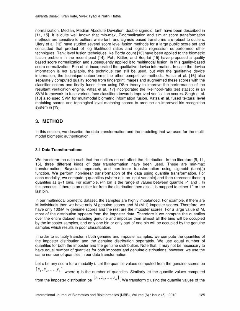
We transform the data such that the outliers do not affect the distribution. In the literature [5, 11, 15], three different kinds of data transformation have been used. These are min-max transformation, Bayesian approach, and non-linear transformation using sigmoid (tanh(.)) function. We perform non-linear transformation of the data using quantile transformation. For each modality, we compute q quantiles (where q is an input variable) and then represent these q quantiles as q+1 bins. For example, i-th bin is the range of values between quantile i-1 and i. In this process, if there is an outlier far from the distribution then also it is mapped to either 1
st or the
last bin. In our multimodal biometric dataset, the samples are highly imbalanced. For example, if there are M individuals then we have only M genuine scores and M (M-1) imposter scores. Therefore, we have only 100/M % genuine scores and the rest are the imposter scores. For a large value of M, most of the distribution appears from the imposter data. Therefore if we compute the quantiles over the entire dataset including genuine and imposter then almost all the bins will be occupied by the imposter samples, and only one bin or only part of one bin will be occupied by the genuine samples which results in poor classification. In order to suitably transform both genuine and imposter samples, we compute the quantiles of the imposter distribution and the genuine distribution separately. We use equal number of quantiles for both the imposter and the genuine distribution. Note that, it may not be necessary to have equal number of quantiles for both imposter and genuine distributions, however, we use the same number of quantiles in our data transformation. Let x be any score for a modality i. Let the quantile values computed from the genuine scores be
],,,[ 21 qyyy K
where q is the number of quantiles. Similarly let the quantile values computed
from the imposter distribution be ],,,[ 21 qzzz K
. We transform x using the quantile values of the

Jayanta Basak, Kiran Kate, Vivek Tyagi & Nalini Ratha
International Journal of Biometrics and Bioinformatics (IJBB), Volume (6) : Issue (5) : 2012 126
genuine distribution to )(xk gen where
1)()( +<≤ xkxk gengen
yxy. If qyx ≥
then 1)( += qxk gen .
Similarly we obtain the transformation of x to )(xk imp using the imposter quantile values ([z]).
We then obtain the resultant transformed score as
)()()( xkxkxk impgen += (1)
Once we obtain the transformed values, we normalize k by 2q+2, i.e., k(x) = k(x)/(2q+2), since k can attain a maximum value of 2q+2. We first compute the transformed scores for the training data. We preserve the quantile information for all modalities derived from the training data. We then perform the model fitting on the transformed training data. For a test sample, we use the quantile information as derived from the training data and transform the test sample in the same way as in Equation (1) using the quantile information from the training data. Ideally, if the genuine samples are separated from the imposter samples for a specific modality then after transformation, the transformed imposters will take values in the range [0,0.5] and the genuine samples will take values in the range [0.5,1]. This is illustrated in Fig. 3. Fig. 2 is the original score distribution of the two of the modalities of the NIST-BSSR1 dataset and Fig. 3 shows the effect of quantile transform on these scores. In the multi-modal score distribution, we can view the transformed scores to be bounded in a four-dimensional hypercube. The imposter samples will be roughly confined in the box defined by [(0, 0, 0, 0), (0.5, 0.5, 0.5, 0.5)] and the genuine samples will occupy rest of the volume. Once we compute the normalized transformed scores, we raise the scores to a certain positive power p i.e.
)()( xkxK p=
where p > 1 (2) With the increase in p, the volume occupied by the imposter samples in the hypercube decreases and the volume occupied by the genuine samples increases. In other words, the imposter sample distribution gets squeezed and the genuine sample distribution expands. This is evident in Fig. 4 which shows the score distribution of the transformed NIST-BSSR1 scores for two of the modalities (the original score distribution is as shown in Fig. 2). We perform the quantile power transformation (QPT) as in Equation (2) and subsequently use linear classifier to classify the multi-modal scores. We denote QPT along with the linear classifier explained in section 3.2 as QPLC.

Jayanta Basak, Kiran Kate, Vivek Tyagi & Nalini Ratha
International Journal of Biometrics and Bioinformatics (IJBB), Volume (6) : Issue (5) : 2012 127
3.2 QPLC Model Fitting We first transform the scores of the training data using the quantile mapping and then normalize
the scores. We then raise the normalized transformed scores to certain positive power and then
perform linear classification. In order to find out the linear classification boundary, it is possible to
perform various techniques which include logistic regression and linear SVM. However, the cost
of misclassification for the genuine samples and imposter samples are not the same in our
classification task. The objective here is to attain the maximum possible TAR with minimum
possible FAR. We restrict the FAR to certain low value and find the optimum classification
boundary to increase TAR as much as possible.
As we mentioned before, we have four different modalities namely the left index, right index, and scores produced by two different matchers. Let us represent the separating hyperplane by
],,,,[ 4321 θwwww where first four parameters define the orientation of the hyperplane in the
four-dimensional space and the last parameter defines the intercept. We constrain the orientation
FIGURE 2: Score distribution of two of the modalities of the NIST-BSSR1 dataset.
FIGURE 3: Quantile transformed score distribution of two of the modalities of the NIST-BSSR1 dataset (before the power transform)

Jayanta Basak, Kiran Kate, Vivek Tyagi & Nalini Ratha
International Journal of Biometrics and Bioinformatics (IJBB), Volume (6) : Issue (5) : 2012 128
parameters as 1
2=w
such that we have four free variables including the intercept. We then perform search over a four-dimensional hypersphere to obtain the orientation parameters. We
search over the hypershpere in steps of certain w∆ , and compute the ROC (FAR vs. TAR) for each such model. We then obtain the set of models which produces the maximum TAR for a certain low FAR (FAR = 0.01%). Once we obtain the set of such models, we compute the AUC (area under the ROC curve) for each such model in the subset. We select one model from the subset which produces the maximum AUC. It is possible that more than one model in the subset produces the maximum AUC, and we randomly select one of such models. The overall approach is shown in Fig. 5. Once we obtain a model computed from the training data, we apply the same model on the test data. We vary the intercept to obtain the ROC on the test data.
3.3 Quantile Transformation Applied To SVM Vector Machine (SVM) classifier has been quite successfully applied to a diverse set of classification problems. To further validate the effectiveness of the proposed QP transformation, we have used the transformed dataset to train a linear kernel SVM [3]. Libsvm [2] library has been used to train the following two linear SVMs.
1. SVM trained on original dataset 2. SVM trained on QP transformed dataset with p = 7
In our experiments we have found that QP transformed SVM performs better than the SVM trained on the original data. This may be attributed to the better suitability of QP transformed data for linear classification. The detailed results are presented in the following section. ====================================
for ,1::01 ww ∆=
2
11 1 wR −=;
for ,::0 12 Rww ∆=
FIGURE 4: QPT transformed score distribution of two of the modalities of the NIST-BSSR1 dataset (p = 7)

Jayanta Basak, Kiran Kate, Vivek Tyagi & Nalini Ratha
International Journal of Biometrics and Bioinformatics (IJBB), Volume (6) : Issue (5) : 2012 129
,1
2
2
2
12 wwR −−=
for 23 ::0 Rww ∆=,
2
3
2
2
2
14 1 wwww −−−=;
compute the ),,,( 4321 wwwwROC
; end end end Obtain the subset W of models from ROC which produces maximum TAR for FAR 0.01%;
for each Wwwww ∈),,,( 4321 ,
compute the ),,,( 4321 wwwwAUC
Select a model vector Ww ∈*
where )(maxarg
*wAUCw Ww∈
=;
==================================
4. RESULTS The performance of the QPLC method was evaluated on a public-domain dataset NIST-BSSR1[1]. This dataset contains multimodal (two fingerprint and two face) scores for 517 users (NIST-517). It also contains two fingerprint matchers’ scores for 6000 persons (NIST-Fingerprint) and two face matchers’ scores for 3000 persons (NIST-Face). The first set of experiments was performed on the multimodal 517 users dataset using 20-fold cross validation. The results reported are the average values over these 20 folds. For the second set of experiments, a larger training dataset was generated for the four modalities by combining the 3000 NIST-Face scores with the first 3000 NIST-Fingerprint scores (We refer to this dataset as NIST-3000). The test dataset used was the 517 sample NIST-Multimodal dataset. We first show that the quantile transformation improves the Receiver Operating Characteristic (ROC) curves even on single modality. For example Fig. 6 displays the ROC on the right index fingerprint distribution for both the original data and the transformed data. We transformed the distribution using a quantile bin of size 4. After transformation, the scores take an approximate uniform distribution. The imposter samples get concentrated in [0, 0.5] and the genuine samples get concentrated in [0.5, 1] (as illustrated in Fig. 3). As discussed in section 3.1, raising the normalized transformed scores to a positive integer power changes the genuine and imposter distributions and we show that this helps the classification. The ROC plots in Fig. 7 and Fig. 8 compare the performance of QPLC with different values of powers for the NIST-multimodal and NIST-3000 datasets respectively. It can be seen that the classification performance improves with the higher values of power for lower values of FAR and then the curves coincide for the higher values of FAR as expected. In Fig. 9 we compare the ROC of the linear SVM, QPT based SVM and Logistic Regression on the NIST-517 dataset. The results indicate that the QPLC achieves significant improvement in the TAR values for low values of FAR as compared to the other techniques. Further, we note that the QPT based SVM performs better than the SVM trained on the original dataset. Fig. 10 shows the
FIGURE 5: Linear classifier of QPLC

Jayanta Basak, Kiran Kate, Vivek Tyagi & Nalini Ratha
International Journal of Biometrics and Bioinformatics (IJBB), Volume (6) : Issue (5) : 2012 130
results of these classifiers on the larger NIST-3000 dataset. These results also show a similar trend as in Fig. 9. The QPLC outperforms other techniques and the QPT based SVM significantly outperforms the SVM trained on the original dataset. The improvement in the SVM performance as a result of the QPT is important since SVM is a widely used scalable classifier.
Table.1 summarizes the TAR values for the FAR of 0.01 percent for all these fusion techniques. In [5] the authors have proposed a likelihood ratio test (LRT) based biometric score fusion. As their results are also based on the 517 sample dataset, we directly compare their LRT based result with the proposed technique in the Table 1. We also directly report the results of a linear classifier based fusion technique [4] on the same dataset. We also compare our transformation to the well known tanh score normalization [11, 15]. We use SVM to classify the tanh transformed scores and the result is reported in Table.1. This result and the results reported in [15] for tanh normalization in combination with different fusion methods on NIST-517 dataset indicate that QPT
FIGURE 7: Comparison of ROC performance on quantile transformed data raised to different values of powers for NIST-517 dataset.
FIGURE 6: Comparison of ROC performance on original data and transformed data for right index
finger print recognition.

Jayanta Basak, Kiran Kate, Vivek Tyagi & Nalini Ratha
International Journal of Biometrics and Bioinformatics (IJBB), Volume (6) : Issue (5) : 2012 131
performs better than tanh normalization. From all the results, we can observe that the performance of QPLC is better than all the other techniques compared.
FIGURE 9: Comparison of ROC performance of QPLC with SVM, SVM + QPT p = 7, and Logistic Regression on the NIST-517 dataset.
FIGURE 8: Comparison of ROC performance on quantile transformed data raised to different values of powers for NIST-3000 dataset.

Jayanta Basak, Kiran Kate, Vivek Tyagi & Nalini Ratha
International Journal of Biometrics and Bioinformatics (IJBB), Volume (6) : Issue (5) : 2012 132
5. CONCLUSIONS In a multimodal score fusion problem, often one has to deal with the scores from the various modalities whose dynamic ranges and probability distributions vary a lot. As a solution to this problem, we have proposed a quantile transformation which is independent of the dynamic ranges of each modality and is not highly susceptible to the outliers. Further we show that raising the normalized quantile values to a power greater than one results in a lower FAR and a higher TAR. Finally, a linear classifier (QPLC) and a SVM trained on the QPT scores significantly outperformed the other classifiers (LRT [5], linear classifier [4] and SVM) that were trained on the original scores confirming the utility of the QPT. We also compared it with other score normalization methods like tanh [11, 15] and found that QPT performs better. QPLC is also designed to particularly handle imbalanced data. We observe that for NIST-3000 dataset, QPLC outperforms other linear classifiers. Since we consider the maximization of AUC explicitly under the constraint of achieving a certain minimum TAR, it is not affected by the imbalance in the samples. The linear classifier of QPLC is constrained by the dimensionality. We
Technique NIST-Multimodal
NIST-3000
LC [4] 99.00 -
GMM [5] 99.10 -
Logistic Regression
98.26 -
SVM + tanh 90.56 -
SVM 98.84 94.19
SVM + QPT 99.03 98.65
QPLC 99.42 99.42
FIGURE 10: Comparison of ROC performance of QPLC with SVM and SVM + QPT p = 7 on the NIST-3000 dataset.
TABLE 1: TAR (%) values for different methods at 0.01% FAR

Jayanta Basak, Kiran Kate, Vivek Tyagi & Nalini Ratha
International Journal of Biometrics and Bioinformatics (IJBB), Volume (6) : Issue (5) : 2012 133
have four modalities and it was possible to design an explicit search mechanism. However, if the dimensionality increases, it may not be possible to perform the explicit search. Overall for relatively low-dimensional dataset and highly imbalanced class samples, QPLC has the potential to outperform the existing classifiers. In this paper, we tested with NIST-BSSR1 dataset, and as a future study we expand the experiments with other multi-modal biometric datasets as well.
6. REFERENCES [1] National Institute of Standards and Technology, NIST Biometric Scores Set – Release 1,
http://www.itl.nist.gov/iad/894.03/biometricscores/, 2004.
[2] Chih-Chung Chang and Chih-Jen Lin, LIBSVM: a library for support vector machines, 2001. Software available at http://www.csie.ntu.edu.tw/~cjlin/libsvm
[3] C. Cortes and V. Vapnik, Support-vector networks, Machine learning, 20(3):273-297, 1995. [4] M. C. Zoepfl and H. J. Korves, Improving identity discovery through fusion, ITPro Jan/Feb
2009. [5] K. Nandakumar, Y. Chen, S. C. Dass, and A. K. Jain, Likelihood ratio based biometric score
fusion, IEEE Trans on Pattern Analysis and Machine Intelligence, Vol. 30, No. 2, Feb 2008. [6] S. Garcia-Salicetti, M.A. Mellakh, L. Allano, and B. Dorizzi, Multimodal biometric score fusion:
the mean rule vs. support vector classifiers, Proc. EUSIPCO, 2005. [7] M. Villegas and R. Paredes, Score Fusion by Maximizing the Area under the ROC Curve,
Pattern Recognition and Image Analysis: 4th Iberian Conference, IbPRIA, June 2009. [8] A. K. Jain, A. Ross, Multibiometric systems, Communications of the ACM, Special Issue on
Multimodal Interfaces 47 (1), 34–40, 2004. [9] J. Kittler, M. Hatef, R. P. Duin, J. G. Matas, On Combining Classifiers, IEEE Transactions on
Pattern Analysis and Machine Intelligence 20 (3), 226–239, 1998. [10] S. Prabhakar, A. K. Jain, Decision-level Fusion in Fingerprint Verification, Pattern
Recognition 35 (4), 861–874, 2002. [11] A. K. Jain, K. Nandakumar, and A. Ross, Score Normalization in Multimodal Biometric
Systems, Pattern Recognition, vol. 38, no. 12, pp. 2270–2285, December 2005. [12] B. Ulery, A. R. Hicklin, C. Watson, W. Fellner, and P. Hallinan, Studies of Biometric Fusion,
NIST, Tech. Rep. IR 7346, September 2006. [13] C. Dwork, R. Kumar, M. Naor and D. Sivakumar, Rank aggregation methods for the Web,
WWW '01: Proceedings of the 10th international conference on World Wide Web, 613-622, 2001.
[14] M. L. Gavrilova and M. M. Monwar, Fusing multiple matcher’s outputs for secure human
identification, Int. J. Biometrics, 1(3), 329-348, 2009. [15] N. Poh, J.V. Kittler, and T. Bourlai, Quality-based score normalization with device qualitative
information for multimodal biometric fusion, IEEE Transactions Systems, Man, and Cybernetics – Part A, 40(3), 539-554, 2010.

Jayanta Basak, Kiran Kate, Vivek Tyagi & Nalini Ratha
International Journal of Biometrics and Bioinformatics (IJBB), Volume (6) : Issue (5) : 2012 134
[16] M. Vatsa, R. Singh, A. Noore, and M. Houck, Quality-augmented fusion of level-2 and level-3 fingerprint information using DSm theory, International Journal of Approximate Reasoning, 50(1), 2009.
[17] M. Vatsa, R. Singh, A. Ross, and A. Noore, Likelihood ratio in a SVM framework: fusing linear and non-linear face classifiers, IEEE Computer Vision and Pattern Recognition Workshop, Anchorage, AK, 1-6, 2008.
[18] R. Singh, M. Vatsa, and A. Noore, “Intelligent Biometric Information Fusion using Support
Vector Machine,” Soft Computing in Image Processing: Recent Advances, M. Nachtegael, D. Weken, E. Kerre, and W. Philips (editors), Springer-Verlag Publishers, 2008.
[19] M. Vatsa, R. Singh, and A. Noore, Improving Iris Recognition Performance using
Segmentation, Quality Enhancement, Match Score Fusion and Indexing, IEEE Transactions on Systems, Man, and Cybernetics - B, 38(3), 2008.
[20] Andrade, C. and von Solms, S. H., Investigating and comparing multimodal biometric
techniques, Policies and Research in Identity Management, IFIP International Federation for Information Processing, vol. 261, pp. 79–90, 2008.

K. K. Senapati, D. R. Das Adhikary & G. Sahoo
International Journal of Biometrics and Bioinformatics (IJBB), Volume (6), Issue (5): 2012. 135
An Application of Pattern Matching for Motif Identification
K. K. Senapati [email protected] Department of Computer Science & Engineering. Birla Institute of Technology, Mesra Ranchi, 835215, India
D. R. Das Adhikary [email protected] Department of Computer Science & Engineering. Birla Institute of Technology, Mesra Ranchi, 835215, India
G. Sahoo [email protected] Department of Information Technology. Birla Institute of Technology, Mesra Ranchi, 835215, India
Abstract
Pattern matching is one of the central and most widely studied problem in theoretical computer science. Solutions to the problem play an important role in many areas of science and information processing. Its performance has great impact on many applications including database query, text processing and DNA sequence analysis. In general Pattern matching algorithms are based on the shift value, the direction of the sliding window and the order in which comparisons are made. The performance of the algorithms can be enhanced to a great extent by a larger shift value and less number of comparison to get the shift value. In this paper we proposed an algorithm, for finding motif in DNA sequence. The algorithm is based on preprocessing of the pattern string(motif) by considering four consecutive nucleotides of the DNA that immediately follow the aligned pattern window in an event of mismatch between pattern(motif) and DNA sequence .Theoretically, we found the proposed algorithms work efficiently for motif identification.
Key words: Pattern Matching, Pattern String, Motif Finding, Motif Identification, Gene Identification, Preprocessing.
1. INTRODUCTION Pattern matching consists in finding one, or more generally, all the occurrences of a given query string (pattern) from a possibly very large text is an old and fundamental problem in computer science. It emerges in applications ranging from text processing and music retrieval to bioinformatics. This task, collectively known as string matching, has several different variations. The most natural and important of these is exact string matching, in which, like the name suggests, one wish to find only occurrences that are exactly identical to the pattern string, which is the focus of our work. The field of approximate string matching, on the other hand find occurrences that are similar to the pattern string. Given a text array, T [1 . . . n], of n character and a pattern array, P [1 . . . m], of m characters. The problem is to find an integer s, called valid shift where 0 ≤s ≤ n - m and T[s +1 . . . s + m] = P [1 . . . m]. In other words, to find whether P in T i.e., where P is a substring of T. The elements of P and T are character drawn from some finite alphabet such as {0, 1} or {A, B ... Z, a, b . . . z} [1] [2]. All pattern-matching algorithms scan the text with the help of a window, which is equal to the length of the pattern. The first process is to align the left ends of the window and the text, and then compare the corresponding characters of the window and the pattern. After a whole match or a mismatch of the pattern, the text window is shifted in the forward direction until the right end of the window reaches the end of the text. The algorithms vary in the order in which character comparisons are made and the distance by which the window is shifted on the text after each attempt. Many pattern matching algorithms

K. K. Senapati, D. R. Das Adhikary & G. Sahoo
International Journal of Biometrics and Bioinformatics (IJBB), Volume (6), Issue (5): 2012. 136
are available with their own merits and demerits based on the pattern length, periodicity and alphabet set. An efficient way is to move the pattern on the text using the best shift value. To this end, several algorithms have been proposed to get a better shift value, for example: Boyer–Moore [3], Quick Search [4], Karp-Rabin [5], Raita [6] and Berry–Ravindran [7]. The efficiency of an algorithm lies in two phases: pre-processing phase and the searching phase. Effective searching phase can be established by altering the order of comparison of characters in each attempt and by choosing an optimum shift value that allows a maximum skip on the text [8]. The difference between various algorithms is mainly due to the shifting procedure and the speed at which a mismatch is detected. The rest of the paper is organized as follows. Section 2 gives the review of several efficient algorithms in practice. Section 3 describes the proposed algorithm in detail. Section 4 is about complexity analysis of the proposed algorithm. In section 5, the experimental results of comparison between proposed algorithm and other compared algorithm are given. And section 6 is the conclusion.
2. PREVIOUS WORK Many promising data structures and algorithms discovered by theoretical community are never implemented or tested at all. This is because the actual performance of the algorithm is not analyzed as only the working of the algorithm in practice is taken care. There have been several pattern matching algorithms designed in the literature till date as discussed below. In the naive or Brute Force technique [1] [2] the string to be searched is aligned to the left end of the text and each pattern character is compared with the corresponding text character. In this process if a mismatch occurs or the pattern character exhausts the pattern is shifted by one unit toward right. The search is again resumed from the start of the pattern until the text is exhausted or match is found. Naturally the number of comparisons being performed is very more as each time the pattern string is shifted right by only one unit towards right. The worst case comparison of the algorithm is O (mn). The number of comparisons can be reduced if we can move the pattern string by more than one unit. This was the idea of KMP algorithm [1][2][9][10]. The KMP algorithm compares the pattern from left to right with the text just as BF algorithm. When a mismatch occurs the KMP algorithm moves the pattern to the right by maintaining the longest overlap of a prefix of the pattern with a suffix of a part of the text that matched the pattern so far. The KMP algorithm does almost 2n text comparisons and the worst case complexity of the algorithm is O (m+n). Boyer-Moore algorithm [2][3] differs from other algorithms in one feature. Instead of comparing the pattern characters from left to right the comparison is done from the right towards left by starting comparison from the rightmost character of the pattern. In case of a mismatch it uses two functions last occurrence function and good suffix function. If the text character does not exist in the pattern then the last occurrence function returns m where m is the length of the pattern string. So the maximum shift possible was m. The worst case running time of the algorithm is O (mn). Quick Search (QS) [2][4] algorithm perform comparisons from left to right order, it's shifting criteria is by looking at one character right to the pattern and by applying bad character shifting rule. The worst case time complexity of QS is same as Horspool algorithm but it can take more steps in practice. Berry Ravindran (BR) [2][7][11] algorithm proposed by Berry and Ravindran, it performs shifts by using bad character shifting rule for two consecutive characters to the right of the partial text window of text string. The preprocessing time complexity is O (m+ (|Σ|) 2) and the searching time complexity is O (mn). In this paper the idea is to reduce the number of comparisons being performed by obtaining as much shift as possible. A shift value of more than length of the pattern is obtained when the pattern gets mismatch with the text for one instance.
3. PROPOSED ALGORITHM The proposed algorithms works in two phases, the preprocessing phase and the searching phase.

K. K. Senapati, D. R. Das Adhikary & G. Sahoo
International Journal of Biometrics and Bioinformatics (IJBB), Volume (6), Issue (5): 2012. 137
3.1. Preprocessing phase In Berry-Ravindran algorithm, two consecutive characters immediately to the right of the pattern window are considered in the function brBc [7]. But in the proposed algorithm, four consecutive characters immediately to the right of window are considered. Initially, the indexes of the four consecutive characters in the text string from the left are (m), (m+1), (m+2) and (m+3) for a, b, c and d respectively. The MBrBc (a, b, c, d) of the algorithm consists in computing for each four characters a, b, c, d for all a, b, c, d , in the pattern. The MBrBc(a, b, c, d) is defined as follows:
MBrBc[a,b,c,d]= min
This function finds the position of the right most occurrence of ‘abcd’ in the pattern and computes shift value so that the ‘abcd’ in the pattern and the ‘abcd’ if any in the text immediately to the right of the window are aligned. If ‘abcd’ does not exist in the pattern or a portion i.e. ‘a’ ‘ab’ ‘abc’ ‘bcd’ ‘cd’‘d’ presents then other cases that are considered. We improve the algorithm in programmatically by using a one dimensional array called shift array (SA). The shift array is use for storing the shift value for all four character permutation of the given pattern. For any four given character we generate a unique number and use this unique number as index to store the shift value for that four character. For any “abcd” the value is cal calculated like this:
index=(a*1000)+( b*100)+( c*10)+d SA [index] =shift value
We use this technique to store the shift value, which is a very efficient than other possible technique. 3.2. Searching Phase In this proposed algorithm, after each attempt the window is shifted to the right using the shift value computed for the four consecutive characters immediately right of the window. MBrBc function calculates the shift value based on the right most occurrences of four consecutive characters, say abcd, which is immediately to the right of the window. The probability occurrence of four consecutive characters, abcd, in the pattern as compared to that of ab is less. Thus MBrBc always provides a better shift than brBc (Berry-Ravindran Bad character function) [12]. The searching phase of the algorithm works in the following way. Step1: Compare the characters of the windows with the corresponding text characters from left as well as right [13][14]. If there is a mismatch during comparison, the algorithm goes to step2, otherwise the comparison process continues until a complete match is found. The algorithm stops and displays the corresponding position of the Pattern on the text string. If we search for all the pattern occurrences in the text string, the algorithm continues to step2. Step2: In this step, we use the shift values from the next arrays depending on the four text characters placed immediately after the pattern window. The window is shifted to the correct positions based on the shift value and the algorithm goes to step 1, this process continues till the end of the string. The searching phase of the algorithm works in the following way. Suppose we have a text string T[O . . . n-l] and pattern P[O . . . m-l] and starts searching of P in T. The algorithm compares the pattern with selected text window from both (right and left) sides simultaneously. In case of match or mismatch MBrBc shift value is used to

K. K. Senapati, D. R. Das Adhikary & G. Sahoo
International Journal of Biometrics and Bioinformatics (IJBB), Volume (6), Issue (5): 2012. 138
shift the window to the right. This procedure is repeated until the window is placed beyond n-m+1, that is the last character of the pattern placed beyond the last character of the text. The Searching Phase of Motif Finding Algorithm 1. Search_Motif(T,P) 2. n�length[T] 3. m�length[p] 4. i�0 5. s�n-m 6. while( i <= s) do 7. left�0 8. right�m-1 9. while(left<=right)do 10. if (P[left]==T[i+left]&& P[right]==T[i+right) 11. left�left+1 12. right�right-1 13. else 14. break 15. end while 16. if(left>right) 17. print “pattern occurs at” T[i]to T[i+m-1] 18. i=i+ MbrBc(T[i+m],T[i+m+1],T[i+m+2],T[i+m+3]) 19. end while 20. end procedur 3.3 Working Example Consider the text and pattern string as shown below where text length n=15 and pattern length m=8 Text (T) = G C A T C G C A G A G A G T A Pattern (P) = G C A G A G A G, m = 8
First Attempt G C A T C G C A G A G A G T A
1 2 Shift=1(MbrBc[G][A][G][A])
G C A G A G A G
Second
Attempt
G C A T C G C A G A G A G T A
1 2 Shift=2(MbrBc[A][G][A][G])
G C A G A G A G
Third Attempt G C A T C G C A G A G A G T A
1 2 Shift=2(MbrBc[A][G][T][A])
G C A G A G A G

K. K. Senapati, D. R. Das Adhikary & G. Sahoo
International Journal of Biometrics and Bioinformatics (IJBB), Volume (6), Issue (5): 2012. 139
First Attempt: In the first attempt, we align the sliding window with the text from the left. In this case, a match occurs between text character (G) and pattern character (G)in the left side of window and a mismatch occurs between text character (A) and pattern character (G)in the right side of window. Therefore we take the immediate four characters following the text as (G,A,G, and A). We find according to MBrBc function. That the shift=1, therefore the window is shifted to the right 1 step. Second Attempt: In the second attempt, we align the sliding window with the text from the left. In this case, a mismatch occurs between text character (C) and pattern character (G)in the left side of window and a match occurs between text character (G) and pattern character (G)in the right side of window. Therefore we take the immediate four characters following the text as (A, G, A and G). We find according to MBrBc function. That the shift=2, therefore the window is shifted to the right 2 step. Third Attempt: In the third attempt, we align the sliding window with the text from the left. In this case, a mismatch occurs between text character (T) and pattern character (G)in the left side of window and a match occurs between text character (G) and pattern character (G)in the right side of window. Therefore we take the immediate four characters following the text as (A, G, T and A). We find according to MBrBc function. That the shift=2, therefore the window is shifted to the right 2 step. Fourth Attempt: In the fourth attempt, we align the sliding window with the text from the left after shift. In this case all the character of the pattern matches with the text. So match performed. Next the window is moved for the next pattern in the text string.
4. ANALYSIS The space complexity is O((m/2+1)).where m is the pattern length..The pre-process time complexity is O(m+|∑|^4). The worst case time complexity is O(nm). The worst case occurs when at each attempt; all the compared characters and the text are matched and at the same time the shift value is equal to 1 i.e. Last character of the pattern is equal to the first character present next to the window. Example: Text (T): AAAAAAAAAAAAAAAAAAAAAAAAAAAAAAAAAAA Pattern (P): AAAAA The best case time complexity is O (n/ (m+2)).The best case occurs when at each attempt; in the first comparison a mismatch is found and at the same time the shift value is m+2. Example: Text (T): AAAAAAAAAAAAAAAAAAAAAAAAAAAAAAAAAAA Pattern (P): SSSSS
5. EXPERIMENTAL EVALUATIONS
To assess the performance of my algorithm, we considered all the well-known algorithms stated before for comparison with the proposed algorithm. The algorithms are compared with test cases and their corresponding results are discussed.
5.1 Environment In the experiments we used a PC with Intel(R) Core(TM) 2 Duo 2.10 and 1.96 GHz processor, with 2GB of RAM. The host operating system is windows Xp. The source codes were compiled using the “gcc” compiler without optimization. All the coding is done with the help of Dev C++ tool.
Fourth
Attempt
G C A T C G C A G A G A G T A
1 3 5 7 8 6 4 2
G C A G A G A G

K. K. Senapati, D. R. Das Adhikary & G. Sahoo
International Journal of Biometrics and Bioinformatics (IJBB), Volume (6), Issue (5): 2012. 140
5.2 Results &Discussion
The plant genome (Arabidopsis thaliana) consists of 27,242 gene sequences distributed over five chromosomes(CHR_I to CHR_V) (NCBI site, ftp://ftp.ncbi.nih.gov/genomes/Arabidopsis_thaliana/CHR_I). Part of a nucleotide sequence of a gene from Chromosome I (CHR_I) has been used (see below for details) to test the proposed algorithm. Two types of data have been analyzed for comparisons; one with small alphabet size, i.e. ∑= 4 (nucleotide sequences) and another with big alphabet size, i.e. ∑ = 20 (amino acid sequences). The algorithms are tested on pattern size 4, 8, 12, 16 and 20.
To assess the performance of our algorithm, we considered two well-known algorithms (i.e. Brute force algorithm and Berry-Ravindran algorithm [5]), the improved version of these two well-known algorithms (i.e. Improved Brute force algorithm and Improved Berry-Ravindran algorithm) for comparison with the proposed algorithm. The Improved Brute Force algorithm is a variation of Brute force algorithm, in which we implement our method of searching in the searching phase. In the same way, we implement our method of searching in the searching phase of Berry-Ravindran [5] algorithm to get the Improved Berry-Ravindran algorithm. The algorithms are compared with test cases and their corresponding results are discussed.
0
50
100
150
200
4 8 12 16 20
Tim
e in
mil
ise
con
d
Size of pattern
Brute Force
Improved Brute Force
Berry-Ravindran
Improved Berry-
Ravindran
proposed algorithm for
motif
Figure 1: Finding Motif in Nucleotide Sequence (time)
0
5000
10000
15000
20000
25000
30000
35000
4 8 12 16 20
no
of
com
pa
riso
n
Size of pattern
Brute Force
Improved Brute Force
Berry-Ravindran
Improved Berry-
Ravindran
proposed algorithm
for motif
Figure 2: Finding Motif in Nucleotide Sequence (character comparison)

K. K. Senapati, D. R. Das Adhikary & G. Sahoo
International Journal of Biometrics and Bioinformatics (IJBB), Volume (6), Issue (5): 2012. 141
0
5000
10000
15000
20000
25000
4 8 12 16 20
no
of
att
em
pt
Size of pattern
Brute Force
Improved Brute Force
Berry-Ravindran2
Improved Berry-
Ravindran
proposed algorithm
for motif
Figure 3: Finding Motif in Nucleotide Sequence (attempt)
0
20
40
60
80
100
4 8 12 16 20
Tim
e in
mil
ise
con
d
Size of pattern
Brute Force
Improved Brute Force
Berry-Ravindran
Improved Berry-
Ravindran
proposed algorithm for
motif
Figure 4: Finding Motif in Amino acid Sequence (time)
0
5000
10000
15000
20000
25000
4 8 12 16 20
no
of
co
mp
ari
so
n
Size of pattern
Brute Force
Improved Brute Force
Berry-Ravindran
Improved Berry-
Ravindran
proposed algorithm for
motif
Figure 5: Finding Motif in Amino acid Sequence (character comparison)

K. K. Senapati, D. R. Das Adhikary & G. Sahoo
International Journal of Biometrics and Bioinformatics (IJBB), Volume (6), Issue (5): 2012. 142
0
5000
10000
15000
20000
25000
4 8 12 16 20
no
of
att
em
pt
Size of pattern
Brute Force
Improved Brute Force
Berry-Ravindran2
Improved Berry-
Ravindran
proposed algorithm
for motif
Figure 6: Finding Motif in Amino acid Sequence (attempt)
From the above figures it is clear that the proposed algorithm takes less number of time, character comparison and attempt in almost all cases, than other to find all the occurrences of the pattern. As the experimental result shows the proposed algorithm is more efficient than other for small pattern and the motif normally ranges between 8 and 20. So it is clear that it is more efficient in finding motif in amino acid sequence as well as nucleotide sequence [15].
6. CONCLUSIONS In this paper we present an efficient pattern matching algorithm based on preprocessing of the pattern string by considering four consecutive characters of the text. The idea of considering four consecutive characters is from the fact that occurrence of three successive characters is less frequent than the other possibilities because of which even the shift value obtained is also more compared to Berry-Ravindran and Brute Force algorithms. The concept of searching from both sides makes the algorithm efficient when a mismatch present at the end of the pattern with that of align text window. Theoretically, we prove that the proposed algorithms will shift the pattern faster than other compared algorithms. Experimentally, we show that the proposed algorithms indeed significantly outperform the compared algorithm in almost all cases.
7. REFERENCES [1] T.H. Cormen, C.E. Leiserson, R.L. Rivest. Introduction to Algorithms, MIT Press, First Edition,
1990, pp. 853-885.
[2] C. Charras, T. Lecroq(1997). Handbook of Exact String Matching Algorithms. [online]. Available: http://www-igm.univ-mlv.fr/~lecroq/string/string.pdf [Oct 08, 2012].
[3] R.S. Boyer, J.S. Moore. A Fast String Searching Algorithm, Communications of the ACM, vol. 20,
pp.762-772, 1977.
[4] D.M. Sunday. A Very Fast Substring Search Algorithm, Journal of Communication of the ACM, vol. 33, pp. 132-142, 1990.
[5] R.M. Karp, M.O. Rabin. Efficient Randomized Pattern Matching Algorithms, IBM J. Res. Dev,
vol. 31, pp. 249-260, 1987.
[6] T.Raita.“Tuning the Boyer-Moore-Horspool string-searching algorithm”, Software – Practice Experience, 1992, pp. 879–884.

K. K. Senapati, D. R. Das Adhikary & G. Sahoo
International Journal of Biometrics and Bioinformatics (IJBB), Volume (6), Issue (5): 2012. 143
[7] T. Berry, S. Ravindran. “A Fast String Matching Algorithm and Experimental Results”, Proceedings of the Stringology Club Workshop’99, 1999, pp. 16-26.
[8] R. Thathoo,A. Virmani, S. Lakshmi, N. Balakrishnan, K. Sekar. TVSBS: A Fast Exact Pattern
Matching Algorithm for Biological Sequences, Current Science, vol. 91, pp. 47-53, Jul. 2006.
[9] D. E. Knuth, H. Morris, V. R. Pratt. Fast Pattern Matching in Strings, SIAM Journal of computing, vol. 6, pp. 323-350, 1977.
[10] J. H. Morris(Jr), V. R. Pratt. “A Linear Pattern Matching Algorithm”, 40th Technical Report,
University of California, Berkeley, 1970.
[11] Y.Huang, L. Ping, X. Pan, G. Cai. “A Fast Exact Pattern Matching Algorithm for Biological Sequences”, International Conference on Biomedical Engineering and Informatics, IEEE computer Society, Feb. 2008, pp. 8-12.
[12] V. Radhakrishna, B. Phaneendra, V.S. Kumar. “A Two Way Pattern Matching Algorithm Using
Sliding Patterns”, 3rd International Conforence on Advanced Computer Theory and Engineering (ICACTE), 2010, vol. 2, pp. 666-670.
[13] Hussain, M. Zubair, J. Ahmed, J. Zaffar. “Bidirectional Exact Pattern Matching Algorithm”,
TCSET’2010, Feb. 2010, pp. 295.
[14] S. S.Sheik,S. K. Aggarwal, A. Poddar, N. Balakrishnan, K. Sekar.A FAST Pattern Matching Algorithm, Journal of Chemical Information and Computer Sciences, vol.44, pp. 1251–1256, 2004.
[15] M.Q. Zhang. “Computational prediction of eukaryotic protein-coding genes”, Nature Reviews
Genetics, vol. 3, Sep. 2002, pp. 698-709.

Danilo Avola, Luigi Cinque & Giuseppe Placidi
International Journal of Biometrics and Bioinformatics (IJBB), Volume (6) : Issue (5) : 2012 144
Medical Image Analysis Through A Texture Based Computer Aided Diagnosis Framework
Danilo Avola [email protected] A
AVI Laboratory
Department of Life, Health and Environmental Sciences University of L’Aquila L’Aquila, Via Vetoio Coppito 2, 67100, Italy
Luigi Cinque [email protected] Department of Computer Science Sapienza University Rome, Via Salaria 113, 00198, Italy
Giuseppe Placidi [email protected] A
AVI Laboratory
Department of Life, Health and Environmental Sciences University of L’Aquila L’Aquila, Via Vetoio Coppito 2, 67100, Italy
Abstract
Current medical imaging scanners allow to obtain high resolution digital images with a complex informative content expressed by the textural aspect of the membranes covering organs and tissues (hereinafter objects). These textural information can be exploited to develop a descriptive mathematical model of the objects to support heterogeneous activities within medical field. This paper presents a framework based on the texture analysis to model the objects contained in the layout of diagnostic images. By each specific model, the framework automatically also defines a connected application supporting, on the related objects, different targets, such as: segmentation, mass detection, reconstruction, and so on. The framework is tested on MRI images and results are reported. Keywords: Medical Imaging, Texture Analysis, Pattern Recognition, Feature Extraction, Framework, Classification, Segmentation, CAD.
1. INTRODUCTION
Current medical imaging scanners, as Magnetic Resonance Imaging (MRI), Position Emission Tomography (PET), or Computer Tomography (CT), allow to obtain digital images with high level detail having a complex informative content that goes beyond the simple visual representation. By observing the relationships between clusters of pixels (i.e., the texture) of the membranes covering objects, meaningful features can be derived to describe the morphological structures of the objects themselves. These features (i.e., textural information) are exploited to develop mathematical models of the objects to support different activities within medical field. In the last years, there have been many efforts to conceive intelligent and automated systems to support critical diagnostic tasks (e.g., analysis, masses identification). Current Decision Support Systems (DSSs), better known as Computer Aided Diagnosis (CAD) systems, are still not completely effective tools. There is an extensive literature focused on the different aspects of the medical image processing. A first remarkable image analysis approach is shown in [1], where the authors describe an automatic segmentation framework, for brain MRI, based on the combination of atlas registration, fuzzy connectedness segmentation, and parametric bias field correction. Another work that has supported some aspects related to the textural image filters is detailed in

Danilo Avola, Luigi Cinque & Giuseppe Placidi
International Journal of Biometrics and Bioinformatics (IJBB), Volume (6) : Issue (5) : 2012 145
[2], presenting a novel co-occurrence matrices based approach to discriminate textures belonging to different kinds of images by considering statistical representation of the structural texture primitives (i.e., textons). Another useful approach is presented in [3], where an approach to automate the myocardial contours detection, to optimize detection and tracking of the grid of tags within myocardium, is described. A further interesting work, [4], presents a real mixed statistical model based on a region-driven curve evolution algorithm. An original approach is described in [5], presenting a novel algorithm to achieve automatic texture based segmentation of organs in MRIs of the abdomen. A robust multi-resolution statistical shape model algorithm is detailed in [6]. A last meaningful paper [7], explores the use of the co-occurrence matrixes to extract textural features from medical images. These approaches are based on several principles related to the image understanding, but there are no works to exploit the morphological structure (given by the texture analysis) of the objects with the aim to provide both their descriptive mathematical model and related dedicated Texture based Computer Aided Diagnosis (T-CAD) Framework. This paper presents some basic technical and methodological advancements of our developed T-CAD Framework which was implemented to perform the texture analysis and reconstruction activities of brain MRI images [8]. These improvements are based on a conceptual generalization of our previous experiences in mathematical modeling of the brain [9], [10] and [11]. More specifically, in this paper we detail the restyled ability of our T-CAD Framework which, on one side, supports the mathematical modeling process of each object represented inside the image layout and, on the other hand, automatically defines, for each model, an ad-hoc application to support a set of fixed targets to aid the medical specialist in a specific context (e.g., craniopharyngioma identification on brain MRI images). Observe that each mathematical model (e.g., craniopharyngioma model) computed during the modeling process is defined one and for all. The effectiveness of the restyled approach is shown both on experimental data (MRI images) and on ad-hoc model-driven applications. The paper is organized as follows. Section 2 illustrates the main architectural aspects of the described T-CAD Framework. Section 3 introduces and discusses the main experimental results, highlighting a specific case study. Section 4 presents the conclusions and plans the future work.
2. THE T-CAD FRAMEWORK ARCHITECTURE
The developed T-CAD Framework is a smart tool that allows skilled user to define a texture based Mathematical Model (MM) of each object represented inside a cluster of diagnostic images representing a volume (in this case, the application is relative to MRI images). A specific MM (e.g., of the brain) is simply the set of formalized mathematical classes representing different basic objects contained in the related image (e.g., cerebral tissue, abnormal mass, background). For each MM the framework supports the building of a dedicated T-CAD system to support a specific medical image analysis process (e.g., image segmentation and mass recognition). The next two sub-sections show the general approach, and the main textural filters used within the framework, respectively. 2.1 The Region Based Algorithm The Region Based Algorithm (RBA) represents the core of the T-CAD Framework. Actually, its main aspect regards the building of the mathematical classes constituting a specific MM, as the dedicated system generation is only a technical application of the related MM on a dataset of source images. For this reason, the definition of the MM will be first detailed, and finally the system generation process will be described. Figure 1 shows the basic architecture of the RBA. The first panel (MRI Scanner and DBs) highlights that the framework works on two kinds of databases (DB). The first (TRaining-DB) is used when the skilled user has to build a new MM. For this reason, the population of the TR-DB follows a rigid protocol which has to ensure the fulfillment of different qualitative and quantitative requirements relatively to the informative content of the related images. The second (SouRce-DB) points out that, once obtained the related MM, it is possible to analyze each kind of source image coming directly from the MRI scanner.
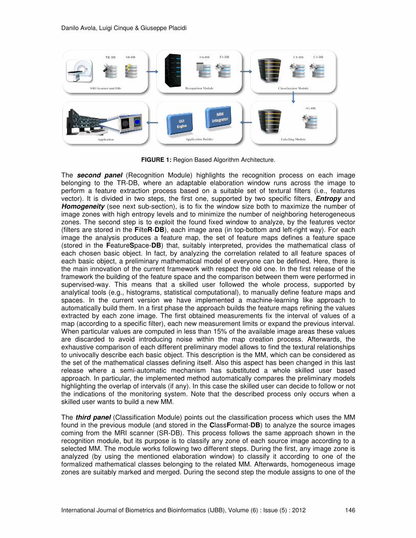
Danilo Avola, Luigi Cinque & Giuseppe Placidi
International Journal of Biometrics and Bioinformatics (IJBB), Volume (6) : Issue (5) : 2012 146
FIGURE 1: Region Based Algorithm Architecture.
The second panel (Recognition Module) highlights the recognition process on each image belonging to the TR-DB, where an adaptable elaboration window runs across the image to perform a feature extraction process based on a suitable set of textural filters (i.e., features vector). It is divided in two steps, the first one, supported by two specific filters, Entropy and Homogeneity (see next sub-section), is to fix the window size both to maximize the number of image zones with high entropy levels and to minimize the number of neighboring heterogeneous zones. The second step is to exploit the found fixed window to analyze, by the features vector (filters are stored in the FilteR-DB), each image area (in top-bottom and left-right way). For each image the analysis produces a feature map, the set of feature maps defines a feature space (stored in the FeatureSpace-DB) that, suitably interpreted, provides the mathematical class of each chosen basic object. In fact, by analyzing the correlation related to all feature spaces of each basic object, a preliminary mathematical model of everyone can be defined. Here, there is the main innovation of the current framework with respect the old one. In the first release of the framework the building of the feature space and the comparison between them were performed in supervised-way. This means that a skilled user followed the whole process, supported by analytical tools (e.g., histograms, statistical computational), to manually define feature maps and spaces. In the current version we have implemented a machine-learning like approach to automatically build them. In a first phase the approach builds the feature maps refining the values extracted by each zone image. The first obtained measurements fix the interval of values of a map (according to a specific filter), each new measurement limits or expand the previous interval. When particular values are computed in less than 15% of the available image areas these values are discarded to avoid introducing noise within the map creation process. Afterwards, the exhaustive comparison of each different preliminary model allows to find the textural relationships to univocally describe each basic object. This description is the MM, which can be considered as the set of the mathematical classes defining itself. Also this aspect has been changed in this last release where a semi-automatic mechanism has substituted a whole skilled user based approach. In particular, the implemented method automatically compares the preliminary models highlighting the overlap of intervals (if any). In this case the skilled user can decide to follow or not the indications of the monitoring system. Note that the described process only occurs when a skilled user wants to build a new MM. The third panel (Classification Module) points out the classification process which uses the MM found in the previous module (and stored in the ClassFormat-DB) to analyze the source images coming from the MRI scanner (SR-DB). This process follows the same approach shown in the recognition module, but its purpose is to classify any zone of each source image according to a selected MM. The module works following two different steps. During the first, any image zone is analyzed (by using the mentioned elaboration window) to classify it according to one of the formalized mathematical classes belonging to the related MM. Afterwards, homogeneous image zones are suitably marked and merged. During the second step the module assigns to one of the

Danilo Avola, Luigi Cinque & Giuseppe Placidi
International Journal of Biometrics and Bioinformatics (IJBB), Volume (6) : Issue (5) : 2012 147
formalized classes, by a statistical distribution algorithm, the remaining zones that have been not classified at all. Each classified image is stored in a new database (ClaSsified-DB). The fourth panel (Labelling Module) highlights the labelling process where every classified source image is properly labelled to provide an immediate visual impact to the user. Each segmented image is arranged in a suitable database (SeGmented-DB). The fifth panel (Application Builder) points out the ad-hoc application builder. In particular, the MM Integrator includes the definition of the selected MM inside the application. Observe that the framework allows user to include more than one specific MM. The GUI Engine highlights that the main mechanisms related to the data presentation (e.g., visualization engine, interaction properties) are the same independently from the specific application. The sixth panel (Application) shows an example of a created application. In this case it is referred to the segmentation of a MRI image of the brain. 2.2 Textural Image Filters The image filters adopted to support the RBA have been suitably chosen and/or created to define the basic textural informative content of the objects composing the human body. Actually, our strong belief is to have found a general approach adoptable for every object represented by MRI images, which, at the moment, has been refined to define the textural morphological structures of four specific objects: brain, heart, liver and bones. Our approach divides the image filters into three different graphical classes, each able to characterize a specific informative layer of the mentioned objects: informative class, texture class and pattern class. The informative class is composed by those first order statistic image filters which distinguish between zones with and without relevant information content. In our experience, the following two set of filters represent the main best suitable ones: N-Order Moment (Mn1) and N-Order Central Moment (Cn2):
∑=
⋅=N
i
n
n ipiM0
),(1
1 ∑
=
⋅−=N
i
n
nn ipMiC0
)()( 2
12 (1)
where: p(i) represents the probability that the gray level i appears inside the elaboration window. The following constraints must hold:
[ ] ,255..01)(0 Ν⊂∈∀≤≤ iip ∑=
Ν∈=N
i
nnip0
21 ,,,1)( 255=N (2)
Mn1 and Cn2 measure respectively, on different textural graphical layers, the consistent quantity and the semantic readability of the information related to different image zones. The texture class is composed by those second order statistic image filters measuring macro and micro textural structures. Our empirical studies allowed to detect the following four set of filters: Homogeneity (Hg(d)), Contrast (Ct(d)), Inverse Difference (Id(d)) and Entropy (En(d)):
[ ] ,),()(0 0
∑∑= =
=N
i
N
j
h
d jipdHg [ ]∑∑= =
⋅−=N
i
N
j
l
d
kjipjidCt
0 0
),()( (3)
[ ],
)(1
),()(
0 0
∑∑= = −+
=N
i
N
js
m
d
ji
jipdId ∑∑
= =
⋅−=N
i
d
N
j
nd jipjipdEn0 0
)),((log),()( (4)

Danilo Avola, Luigi Cinque & Giuseppe Placidi
International Journal of Biometrics and Bioinformatics (IJBB), Volume (6) : Issue (5) : 2012 148
where: pd(i,j) represents the probability that two points with distance d have respectively i and j gray value. The following constraints must hold:
[ ] [ ] 2255..0255..0),(1),(0 Ν⊂×∈∀≤≤ jijipd (5)
,1),(0 0
=∑∑= =
N
i
N
j
d jip [ ] ,8..1 Ν⊂∈d ,,,,,, Ν∈snmlkh 255=N (6)
Hg(d) measures the degree of uniformity of the different image zones, where high or low values within the feature maps highlight light or wide changes of the textural structures, respectively. Ct(d) expresses roughly how the mentioned structural changes occur. High values of the related feature maps, point out fast continuous changes within the image zones. On the contrary, slow changes are highlighted by low values. Id(d) provides the measure of the transition between different basic objects, where low values typically highlight a boundary zone. En(d) is used to detect the randomness level within the considered image zone, where the complex changes in the random distribution of the grey levels are directly proportional to the given values. The pattern class is composed by those second order statistic image filters measuring pattern structures. Experimental observations allowed to identify the following two set of filters: Correlation (Cr(d)) and Difference Entropy (De(d)):
,)(
),()()()(
0 0
∑∑= = ⋅
⋅−⋅−=
N
i
N
ja
yx
p
dyx jipjidCr
σσ
µµ[ ]∑
=
−−−=N
i
yxnyx ipipdDe0
)(log)()( (7)
where:
,)),((0 0
∑∑= =
⋅=N
i
N
j
dx jipiµ ∑∑= =
⋅−=N
i
N
j
dxx jipi0 0
2 )),(()( µσ (8)
,)),((0 0
∑∑= =
⋅=N
i
N
j
dy jipjµ ∑∑= =
⋅−=N
i
N
j
dyy jipj0 0
2 )),(()( µσ (9)
and, in addition to the constraints shown in (5) and (6), the following ones must hold:
[ ] ,),()(0 0
∑∑= =
− =N
i
N
j
g
dyx jipkp ,kji =− Ν∈kgnap ,,,, (10)
Cr(d) is usually used to recognize definite patterns within texture zones previously identified, while the De(d) is adopted to detect the different components (i.e., parts of a same pattern) of different basic objects. Each class of filters is based on the variation of the current co-occurrence matrix concept, where the elaboration process considers all the search directions. In particular, each couple of pixels, able to increase a coefficient of the matrix, is chosen considering a pixel (i.e., the center of a circle) within the elaboration window and the connected pixel which is at the boundary of the circumference related to the fixed radius (i.e., the d parameter). The parameters belonging to the set of filters are customized, within the recognition process, according to the specific contextual medical domain and related tasks. Besides, the shown filters are often used on more than one level of the Gaussian Pyramid [12] to enrich the resolution of the texture described by the MMs.

Danilo Avola, Luigi Cinque & Giuseppe Placidi
International Journal of Biometrics and Bioinformatics (IJBB), Volume (6) : Issue (5) : 2012 149
3. EXPERIMENTAL RESULTS AND A CASE STUDY This section summarizes the experimental results regarding the analysis of MRI images of different body districts: brain, heart, liver and bones. To explain the experimental session, the following three general tasks have been selected according to the present medical image analysis process: task 1 - layout segmentation, task 2 - abnormal mass or lesion detection, task 3 - textural characterization. Table 1 reports the experimental session which has been divided in two different phases. The first, regarding MRI image recognition, has concerned the selection of patients (455) to define the set of training images (1850) and to build the four basic MMs. The second, regarding the MRI image classification and segmentation, has concerned the selection of patients (615) to obtain a set of images (2565) to test each MM on the mentioned tasks.
Medical Domain
Training Patients
Testing Patients
Training DB Images Source DB Images Partial Images Task 1 Task 2 Task 3 Task 1 Task 2 Task 3
Brain 270 385 450 680 60 975 775 40 2980
Heart 75 100 150 80 35 170 100 25 560 Liver 60 80 70 100 30 135 90 20 445
Bones 50 50 70 85 40 100 100 35 430
Total Images
---------- ---------- 740 945 165 1380 1065 120 4415
TABLE 1: Main Case Studies: Training and Source DB.
Actually, the best qualitative results (more than 90% of success rate) come from the brain MM which has a large amount of training and test images. Moreover, it has been our historical first study case. Also the remaining three models have a high success rate (between the 65% and 80%), but they need for wider experimental sessions. In fact, the accuracy of the MM is strongly tied to the amount of training images used to refine the mathematical classes. To show more details about a specific segmentation process next sub-section shows a case study regarding the segmentation of the brain images. 3.1 Case Study: MRI Brain Images This section shows a concrete case study in which a suitable mathematical model is defined according to specific targets, and where a model-based application is created to support the related image analysis process. Actually, the framework produces the same application in which only the mathematical model is replaced each time. The morphological structures of objects are very different, each of them can be better emphasized according to a specific kind of MRI image (e.g., T1, T2, Proton Density (PD)). For this reason, a brief specification of the DICOM (Digital Imaging and Communication in Medicine) image format is given in relation to a specific case study. The Brain Mass Identification (BMI) application has been created to aid medical specialists during the mass identification within the brain MRI images. In particular, the following targets were established:
a. segmentation of the image layout in three basic objects: cerebral tissue, rest of the image (i.e. muscular and bones) and background;
b. identification within the cerebral tissue of abnormal masses (e.g., gliomas, craniopharyngiomas, medulloblastomas);
c. classification of the found abnormal masses distinguishing them from other kinds of primary cerebral tumors.
A careful analysis of the set of pixels composing brain MRI images detected in the transversal T1
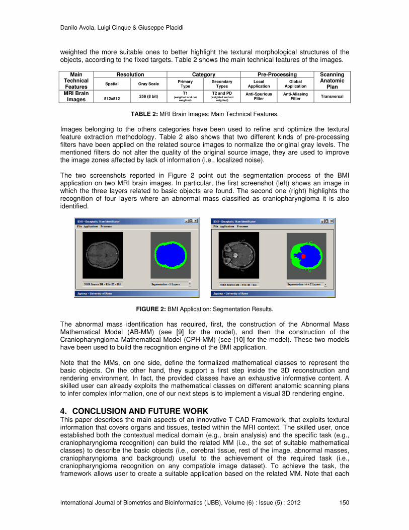
Danilo Avola, Luigi Cinque & Giuseppe Placidi
International Journal of Biometrics and Bioinformatics (IJBB), Volume (6) : Issue (5) : 2012 150
weighted the more suitable ones to better highlight the textural morphological structures of the objects, according to the fixed targets. Table 2 shows the main technical features of the images.
Main Technical Features
Resolution Category Pre-Processing Scanning Anatomic
Plan Spatial Gray Scale
Primary Type
Secondary Types
Local Application
Global Application
MRI Brain Images
512x512
256 (8 bit) T1
(weighted and not weighted)
T2 and PD (weighted and not
weighted)
Anti-Spurious Filter
Anti-Aliasing Filter
Transversal
TABLE 2: MRI Brain Images: Main Technical Features.
Images belonging to the others categories have been used to refine and optimize the textural feature extraction methodology. Table 2 also shows that two different kinds of pre-processing filters have been applied on the related source images to normalize the original gray levels. The mentioned filters do not alter the quality of the original source image, they are used to improve the image zones affected by lack of information (i.e., localized noise). The two screenshots reported in Figure 2 point out the segmentation process of the BMI application on two MRI brain images. In particular, the first screenshot (left) shows an image in which the three layers related to basic objects are found. The second one (right) highlights the recognition of four layers where an abnormal mass classified as craniopharyngioma it is also identified.
FIGURE 2: BMI Application: Segmentation Results.
The abnormal mass identification has required, first, the construction of the Abnormal Mass Mathematical Model (AB-MM) (see [9] for the model), and then the construction of the Craniopharyngioma Mathematical Model (CPH-MM) (see [10] for the model). These two models have been used to build the recognition engine of the BMI application. Note that the MMs, on one side, define the formalized mathematical classes to represent the basic objects. On the other hand, they support a first step inside the 3D reconstruction and rendering environment. In fact, the provided classes have an exhaustive informative content. A skilled user can already exploits the mathematical classes on different anatomic scanning plans to infer complex information, one of our next steps is to implement a visual 3D rendering engine.
4. CONCLUSION AND FUTURE WORK
This paper describes the main aspects of an innovative T-CAD Framework, that exploits textural information that covers organs and tissues, tested within the MRI context. The skilled user, once established both the contextual medical domain (e.g., brain analysis) and the specific task (e.g., craniopharyngioma recognition) can build the related MM (i.e., the set of suitable mathematical classes) to describe the basic objects (i.e., cerebral tissue, rest of the image, abnormal masses, craniopharyngioma and background) useful to the achievement of the required task (i.e., craniopharyngioma recognition on any compatible image dataset). To achieve the task, the framework allows user to create a suitable application based on the related MM. Note that each

Danilo Avola, Luigi Cinque & Giuseppe Placidi
International Journal of Biometrics and Bioinformatics (IJBB), Volume (6) : Issue (5) : 2012 151
MM is defined once and for all. At the moment, our main work is to refine the MM of the following organs and tissues: brain, heart, liver and bones. Another goal is the development of a rendering engine to renderize and visualize 3D objects reconstruction.
5. REFERENCES [1] Y. Zhou and J. Bai. “Atlas-Based Fuzzy Connectedness Segmentation and Intensity
Nonuniformity Correction Applied to Brain MRI.” IEEE Transaction on Biomedical Engineering. Sponsored by IEEE Engineering in Medicine and Biomedicine Society, IEEE CS Press, 54(1), pp. 122-129, 2007.
[2] Q. Li and Z. Shi. “Texture Image Retrieval Using Compact Texton Co-Occurrence Matrix
Descriptor.” In Proceedings of the 11th ACM International Conference on Multimedia Information Retrieval (MIR'10, March 29-31), USA, ACM Press, 2010, pp. 83-90.
[3] A. Histace, B. Matuszewski and Y. Zhang. “Segmentation of Myocardial Boundaries in
Tagged Cardiac MRI Using Active Contours: A Gradient-Based Approach Integrating Texture Analysis.” International Journal of Biomedical Imaging (IJBI'09), Hindawi Publishing Corporation, pp. 1-8, 2009.
[4] J. Niranjan and B. Michael. “Non-Parametric Mixture Model Based Evolution of Level Sets
and Application to Medical Image.” International Journal of Computer Vision (IJCV'10), Springer Verlag, 88(1), pp. 52-68, 2010.
[5] J. Wu, S. Poehlman, M.D. Noseworthy and M.V. Kamath. “Texture Feature Based
Automated Seeded Region Growing in Abdominal MRI Segmentation.” Journal in Biomedical Science and Engineering (JBiSE'09), Research Publishing, vol. 2, pp. 1-8, 2009.
[6] J. Schmid, J. Kim and N. Magnenat-Thalmann. “Robust Statistical Shape Models for MRI
Bone Segmentation in Presence of Small Field of View.” International Journal of Medical Image Analysis (IJMIA'11), 15(1), pp. 155-168, 2011.
[7] L. Tesar, D. Smutek, A. Shimizu and H. Kobatake. “Medical Image Segmentation Using
Co-Occurrence Matrix Based Texture Features Calculated on Weighted Region.” In Proceedings of the 3th Conference on IASTED International Conference: Advances in Computer Science and Technology (ACST'07), ACTA Press, 2007, pp. 243-248.
[8] D. Avola, L. Cinque and M. Di Girolamo. “A Novel T-CAD Framework to Support Medical
Image Analysis and Reconstruction”. In Proceedings of the 16th International Conference on Image Analysis and Processing (ICIAP’11), Springer-Verlag vol. 6979, 2011, pp. 414-423.
[9] D. Avola and L. Cinque. “Encephalic NMR Image Analysis by Textural Interpretation.” In
Proceedings of the 2008 ACM Symposium on Applied Computing. Wainwright (SAC’08, March 16-20), ACM Press, 2008, pp. 1338-1342.
[10] D. Avola and L. Cinque. “Encephalic NMR Tumor Diversification by Textural Interpretation.
In Proceedings of the 15th International Conference on Image Analysis and Processing (ICIAP'09), Springer-Verlag, vol.5716, 2009, pp. 394-403.
[11] D. Avola, L. Cinque and M. Di Girolamo. “Texture Based Approaches to Support Medical
Image Analysis. Internal Technical Report in Medical Image Proessing. DSI - Sapienza University of Rome, ITR-MIP '10, Int. Res. on Medical Imaging, 2010.

Danilo Avola, Luigi Cinque & Giuseppe Placidi
International Journal of Biometrics and Bioinformatics (IJBB), Volume (6) : Issue (5) : 2012 152
[12] D.J. Heeger and J.R. Bergen. “Pyramid-Based Texture Analysis/Synthesis.” In Proceeding of 22th Annual Conference on Computer Graphics and Interactive Techniques (SIGGRAPH'95), NY, USA, ACM Press, 1995, pp. 229-238.

INSTRUCTIONS TO CONTRIBUTORS The International Journal of Biometric and Bioinformatics (IJBB) brings together both of these aspects of biology and creates a platform for exploration and progress of these, relatively new disciplines by facilitating the exchange of information in the fields of computational molecular biology and post-genome bioinformatics and the role of statistics and mathematics in the biological sciences. Bioinformatics and Biometrics are expected to have a substantial impact on the scientific, engineering and economic development of the world. Together they are a comprehensive application of mathematics, statistics, science and computer science with an aim to understand living systems. We invite specialists, researchers and scientists from the fields of biology, computer science, mathematics, statistics, physics and such related sciences to share their understanding and contributions towards scientific applications that set scientific or policy objectives, motivate method development and demonstrate the operation of new methods in the fields of Biometrics and Bioinformatics. To build its International reputation, we are disseminating the publication information through Google Books, Google Scholar, Directory of Open Access Journals (DOAJ), Open J Gate, ScientificCommons, Docstoc and many more. Our International Editors are working on establishing ISI listing and a good impact factor for IJBB. The initial efforts helped to shape the editorial policy and to sharpen the focus of the journal. Starting with Volume 6, 2012, IJBB will appear with more focused issues related to biometrics and bioinformatics studies. Besides normal publications, IJBB intend to organized special issues on more focused topics. Each special issue will have a designated editor (editors) – either member of the editorial board or another recognized specialist in the respective field. We are open to contributions, proposals for any topic as well as for editors and reviewers. We understand that it is through the effort of volunteers that CSC Journals continues to grow and flourish.
LIST OF TOPICS The realm of International Journal of Biometrics and Bioinformatics (IJBB) extends, but not limited, to the following:
• Bio-grid • Bio-ontology and data mining
• Bioinformatic databases • Biomedical image processing (fusion)
• Biomedical image processing (registration) • Biomedical image processing (segmentation)
• Biomedical modelling and computer simulation
• Computational genomics
• Computational intelligence • Computational proteomics
• Computational structural biology • Data visualisation
• DNA assembly, clustering, and mapping • E-health
• Fuzzy logic • Gene expression and microarrays
• Gene identification and annotation • Genetic algorithms
• Hidden Markov models • High performance computing
• Molecular evolution and phylogeny • Molecular modelling and simulation
• Molecular sequence analysis • Neural networks

CALL FOR PAPERS Volume: 7 - Issue: 1 i. Paper Submission: November 30, 2012 ii. Author Notification: December 31, 2012
iii. Issue Publication: January 2013

CONTACT INFORMATION
Computer Science Journals Sdn BhD
B-5-8 Plaza Mont Kiara, Mont Kiara
50480, Kuala Lumpur, MALAYSIA
Phone: 006 03 6204 5627
Fax: 006 03 6204 5628
Email: [email protected]