
International Journal Business of and Finance ESEARCH CONTENTS Individual Investors’ Participation...
113
R The International Journal of Business and Finance ESEARCH CONTENTS Individual Investors’ Participation and Divergence of Opinion in New Issue Markets: Evidence from Malaysia 1 Cheedradevi Narayanasamy, Izani Ibrahim & Yeoh Ken Kyid The Effect of Real Exchange Rate Volatility on Exports in the Baltic Region 23 Carlos Moslares & E. M. Ekanayake Label Co-Movement: Component Stock Inclusion and Exclusion Between Different Exchange-Traded Funds 39 Chun-An Li, Min-Ching Lee & Ju-Hua Liu Determinants and Marginal Value of Corporate Cash Holdings: Financial Constraints Versus Corporate Governance 57 Wenchien Liu Working Capital Variations by Industry and Implications for Profitable Financial Management 71 Walid Masadeh, Ahmad Y. A. Khasawneh & Wasfi AL Salamat The Effect of Dow Jones Industrial Average Index Component Changes on Stock Returns and Trading Volumes 81 Eric C. Lin Corporate Governance and Product Market Power: Evidence from Taiwan 93 Chong-Chuo Chang, Shieh-Liang Chen, Aini Farmania, Feng-Tse Tsai & Ping-Chao Wu VOLUME 12 2018 NUMBER 1
Transcript of International Journal Business of and Finance ESEARCH CONTENTS Individual Investors’ Participation...

RThe International Journal of
Business and FinanceESEARCH
CONTENTS
Individual Investors’ Participation and Divergence of Opinion in New Issue Markets: Evidence from Malaysia 1Cheedradevi Narayanasamy, Izani Ibrahim & Yeoh Ken Kyid
The Effect of Real Exchange Rate Volatility on Exports in the Baltic Region 23Carlos Moslares & E. M. Ekanayake
Label Co-Movement: Component Stock Inclusion and Exclusion Between Different Exchange-Traded Funds 39Chun-An Li, Min-Ching Lee & Ju-Hua Liu
Determinants and Marginal Value of Corporate Cash Holdings: Financial Constraints Versus Corporate Governance 57Wenchien Liu
Working Capital Variations by Industry and Implications for Profitable Financial Management 71Walid Masadeh, Ahmad Y. A. Khasawneh & Wasfi AL Salamat
The Effect of Dow Jones Industrial Average Index Component Changes on Stock Returns and Trading Volumes 81Eric C. Lin
Corporate Governance and Product Market Power: Evidence from Taiwan 93Chong-Chuo Chang, Shieh-Liang Chen, Aini Farmania, Feng-Tse Tsai & Ping-Chao Wu
VOLUME 12 2018NUMBER 1

The International Journal of Business and Finance Research
Turki Alzomaia King Saud UniversityJames E. Briley Northeastern State UniversitySalem Lotfi Boumediene Montana State University BillingsSurya Chelikani Quinnipiac UniversityYahn-Shir Chen University of Science and TechnologyE.M. Ekanayake Bethune-Cookman UniversityGary M. Fleischman Texas Tech UniversityHan-Ching Huang Chung Yuan Christian UniversityStoyu Ivanov San José State UniversityLynda S. Livingston University of Puget SoundGulser Meric Rowan University
Rajesh Mohnot Middlesex UniversityLinda Naimi Purdue UniversityDev Prasad University of Massachusetts LowellCharles Rambo University of NairobiEduardo Sandoval Universidad De ConcepcionJonathan Stewart Abilene Christian UniversityDirk Swagerman University of GroningenRanjini Thaver Stetson UniversityGianfranco A. Vento Regent’s CollegeMatthew Walker Southwest Minnesota State UniversityDevrim Yaman Western Michigan University
Editorial Board
Editor in ChiefTerrance Jalbert
Managing EditorMercedes Jalbert
The International Journal of Business and Finance Research, ISSN: 1931-0269 (print) and ISSN 2157-0698 (online), publishes high-quality articles in all areas of finance, accounting and economics. Theoretical, empirical and applied manuscripts are welcome for publication consideration. The Journal is published five times per year by the Institute for Business and Finance Research, LLC. All papers submitted to the Journal are blind reviewed. The Journal is distributed in print and through EBSCOhost, SSRN, and RePEc. The Journal is also indexed in the American Economic Association’s Econlit, e-JEL, and JEL on CD, and Colciencias.
The views presented in the Journal represent opinions of the respective authors. The views presented do not necessarily reflect the opinion of the editors, editorial board or staff of the Institute for Business and Finance Research, LLC. The Institute actively reviews articles submitted for possible publication. However, the Institute does not warrant the correctness of information provided in the articles or suitability of information in the articles for any purpose.
This Journal is the result of the collective work of many individuals. The Editors thank the members of the Editorial Board, ad-hoc reviewers and individuals that have submitted their research to the Journal for publication consideration.
ISSN : 1931-0269 (print) and ISSN: 2157-0698 (online)
All Rights Reserved . The Institute for Business and Finance Research, LLC
The International Journal of Business and Finance Research Vol. 12, No. 1, 2018, pp. 1-22 ISSN: 1931-0269 (print) ISSN: 2157-0698 (online)
www.theIBFR.com
1
INDIVIDUAL INVESTORS’ PARTICIPATION AND
DIVERGENCE OF OPINION IN NEW ISSUE MARKETS: EVIDENCE FROM MALAYSIA
Cheedradevi Narayanasamy, Nilai University Malaysia Izani Ibrahim, Prince Sultan University, Riyadh
Yeoh Ken Kyid, The University of Nottingham, Malaysia Campus
ABSTRACT We investigate the effects of individual investors’ participation on after-market divergence of opinion (DOP) for 269 Malaysian fixed-price initial public offerings (IPOs). Our findings show that individual investor participation moderates the relationship between initial performance and after-market investors’ opinion. Furthermore, our findings suggest that individual investors who participate in initial public offerings dispose their holdings quickly to take advantage of DOP in the after-market. However, the after-market investors are not willing to pay higher for IPOs sold by the participating individual investors. Our analysis across market conditions shows that the initial performance of IPOs with greater individual investor participation in (i) hot issues is inversely related to after-market DOP and, (ii) cold issues is positively related to after-market DOP (indicating signs of aversion to losses). JEL: G02, G11, G14, G18, G12, L10 KEYWORDS: Divergence of Opinion, Individual Investors’ Participation, Post-IPO Performance, Offer
Turnover, Underpriced IPOs, Loss Aversion INTRODUCTION
ehavioral finance embodies the notion that individual cognitive biases influence investors’ trades in financial markets. For instance, a number of past studies have clearly established that individual cognitive biases affect investors’ heterogeneous beliefs regarding the distribution of future returns
on equity investments. Consequently, market outcomes are partially determined by individual investors’ aggregated equity trading behavior. The different ways by which individual investors update their respective beliefs about the distribution of future returns is termed as divergence of opinion (Wang and Liu, 2014, and Miller, 1977). The divergence of opinion (DOP) phenomenon is typically captured by the changes in trading volume of a particular equity following an event (Miller, 1977, Karpoff, 1986, Harris and Raviv, 1993, Kandel and Pearson, 1995, Hong and Stein, 2007, Garfinkel 2009, and Wang and Liu, 2014). Many past empirical studies have shown that DOP is typically greater in new issue markets such asinitial public offerings (IPOs). However, most of the past studies scrutinize on the effects of DOP on the underpricing of IPOs, while studies on volume behavior is relatively scarce. For the few studies that scrutinized on volume behavior, the findings suggest that higher flipping of institutional trade lead to lower post-IPO performance. Even though institutional investors involved in the flipping of IPO only account for a relatively small proportion of overall trading volume in the after-market. (Krigman, Shaw and Womack, 1999, Aggarwal 2003, Bayley, Lee and Walter, 2006, Ellis, 2006, and Boehme and Colak, 2012). Overall, the relationship between the
B

C. Narayanasamy et al | IJBFR ♦ Vol. 12 ♦ No. 1 ♦ 2018
2
participation of individual investors and after-market DOP within the context of IPOs is under researched even though they constitute key elements of volume behavior. As a response to the paucity of research identified, we scrutinize on the DOP phenomenon and individual investors participation in an emerging market setting. In this regard, we have chosen the Malaysian IPO market as the volume of trading activity is much greater compared to other emerging markets in Asia. Furthermore, recent studies have shown that the IPO turnover ratio in Malaysia is on a rising trend (from 7% as reported by Chong, Ali and Ahmad, 2009 to 77% as reported by Low and Yong, 2013) while initial performance has declined from a previous high of 166% (see Dawson, 1987) to as low as 26.54% (see Low and Yong, 2013). In addition, the first-year post-IPO performance is relatively low for instance, Dawson, (1987) reported an 18.2% increase, Paudyal, Saadouni and Briston, (1998) obtained a figure of 2.4%, and Ahmad-Zaluki and Lim, (2012 ) reported 12.54%). In comparison, empirical studies on DOP in Western capital markets reported considerably lower volume movements on the first day. For instance, in the US, the median and mean IPO turnover ratios were between 33% to 81.97% (Krigman, et al. 1999, Aggarwal, 2003). In Australia, the mean IPO turnover ratio was 22% (see Bayley et al. 2006), 24% for Greece and 20% for France (see Chahine, 2007). In Malaysia, the rising trading volume followed by declines of both initial as well as post-IPO performance suggests that investors may be facing difficulties in estimating the values of new offerings. Another valid consideration is the fact that fixed-price offers dominate the Malaysian IPO market, primarily due to the fact that such offers are favoured by individual investors (Chowdhry and Nanda, 1996). This observation is unsurprising as a large number of individual investors participate in the Malaysian equity market (see, Chong, 2009, Chong et al., 2009). These individual investors are more prone to the effects of DOP as they tend to be less knowledgeable (Yong, 2010, Chong, 2009). These distinctive characteristics provide added justification for our choice of investigating the DOP phenomenon amongst investors in the Malaysian IPO market. Moreover, Bayley et al. (2006) have demonstrated that IPOs with greater individual investor participation actually perform better in the long-run. It must be noted that the greater importance accorded to the role of individual investors is a fairly recent development as, traditionally, these investors are dismissed as being largely noise traders that have little importance. In summary, our paper investigates the role individual investors in the Malaysian IPO market as well as the influence of their participation on the after-market DOP. LITERATURE REVIEW From the behavioral perspective, divergence of opinion (DOP) can occur as investors update their beliefs through a myriad of ways (Goetzmann & Massa, 2005), and the resulting differences generate large volume movements in the capital markets (see Wang and Liu, 2014, Garfinkel, 2009, Hong and Stein, 2007, Goetzmann and Massa, 2005, Kandel and Pearson, 1995, Harris and Raviv, 1993, and Karpoff, 1986). In addition, many academics contend that investors’ opinions tend to diverge more significantly when it comes to IPOs as compared to ‘seasoned’ stocks in the market (see, for example, Boehme and Colak, 2012, Gao, Mao and Zhong, 2006, Diether, Malloy and Scherbina, 2002). Here, differences in beliefs that investors hold will trigger disagreements about the future distributions of IPO returns in the after-market, which induces excessive trading. Since the after-market investors are faced with a choice of either buying the IPOs or other investment choices available in the market, their trading is likely to be impacted by the attention on pertinent IPO characteristics. According to Chahine (2007) and Chong et al. (2009), investors will be attracted to buy IPOs with a greater pre-market interest, despite the higher premiums typically attached to such offers. When it comes to IPOs, individual investors are also unlikely to hold their optimal allocation of shares especially for longer periods. According to Ellis (2006), high volumes of trading occur when an IPO’s original long-

The International Journal of Business and Finance Research ♦ VOLUME 12 ♦ NUMBER 1 ♦ 2018
3
term investors adjust their portfolios to optimal positions. In addition, IPOs that are many times over-subscribed may also spur the rationing of allocations. For instance, some investors may wish to accumulate more shares, as they may have received only a portion of their desired holdings in the allocation process. On the other hand, others may wish to liquidate (flip) their respective allocations at prices higher than the offer price rather than build up their holdings (at higher market prices). The attention that these investors show is best reflected by the subscription ratio. Greater subscription ratio indicates that there is greater attention in the primary market, and this could have an impact on the opinion formed in the after-market. In this regard, Chahine (2007) show a positive weak association between the subscription ratio and after-market DOP of fixed-price IPOs. However, Low and Yong (2013) found an insignificant relationship between the subscription ratio and turnover ratio. Nevertheless, we hypothesize (H1) that the subscription ratio, which captures pre-market investors’ interest, positively relates to after-market DOP with higher participation of individual investors. Overall volume behavior is assumed to be a result of persistent early trading which eventually depresses prices over the long-run. However, Bayley et al. (2006) and Chong et al. (2009) argue that greater offer turnover on the first-day of trading is positively related to post-IPO performance. In contrast, Krigman et al. (1999), Houge, Loughran, Yan and Suchanek (2001) and Gounopoulos (2006) found that lower turnover IPOs in initial trading would result in significant outperformance when compared to those with higher turnover after a year of trading. Similarly, Boehme and Colak (2012) support this relationship between turnover and post-IPO performance. An alternative argument is that such a phenomenon is possibly attributed to the type of participants. This is because, in the US, the participation of institutional investors is greater in new share offerings. In fact, US-based offerings are made using the book-building method, which gives greater discretion for underwriters to allocate shares. There is greater tendency for the underwriters to allocate shares to their desired clients, who are mostly institutional investors (see Loughran & Ritter, 2004). However, in emerging markets with greater number of fixed-price IPOs, underwriters do not have such discretion (see Yong 2007). This situation can create more disagreements about IPO value in the after-market. Moreover, fixed-price IPOs dominate new share issues in emerging capital markets (Low & Yong, 2013). Within such a context, individual investors who are usually not well informed tend to play a more active role (Aggarwal, Prabhala and Puri, 2002, Yong, 2010, Chong et al. 2009, Miller and Reilly, 1987, Rock 1986, Chowdhry and Nanda, 1996). These investors are likely to end up with overpriced IPOs, which remain after the underpriced IPOs are fully subscribed by the informed investors in the primary market (Miller and Reilly, 1987). Moreover, disagreements relating to offers held by individual subscribers are expected to be more pronounced when the IPOs start trading. In the case of Malaysia, IPOs that are more severely underpriced were documented to be allocated to individual investors (Jelic, Saadouni & Briston, 2001, How, Jelic, Saadouni and Verhoeven, 2007). Here, we hypothesize (H2) that the participation of individual investors moderates the relationship between initial performance and after-market DOP. The opinion of individual investors in the IPO after-market is likely to be influenced by other cognitive/physiological biases (see Kaustia, 2004, Bayley et al., 2006, Chong, 2009, Chong, Ahmad and Ali, 2011). As investment evaluation and decision-making are often complex processes, individual investors will likely resort to information processing “shortcuts” that are derived mainly from their past experiences. Kahneman and Tversky (1982) made use of the term heuristic simplification to describe this tendency to use rules of thumb to simplify complex scenarios in decision-making. The underlying presumption is that individual investors are cognitively constrained to deal with complicated investment-related information or to process wide sets of information/tasks. Even though heuristics is likely to result in errors, it is nevertheless used as a way of choosing between investment alternatives particularly when the degree of uncertainty is high. Investors typically use their past experiences as the information processing shortcuts termed as representative heuristic. Representative heuristic (Tversky and Kahneman,1974, Kahneman and Tversky,

C. Narayanasamy et al | IJBFR ♦ Vol. 12 ♦ No. 1 ♦ 2018
4
1982) is a judgement about probability of an event occurring or identification based on its similarity to a corresponding type of event, object or process. When viewed as a device for simplifying the process of choosing between alternatives particularly under uncertain conditions, heuristic representation have been shown to influence investors’ beliefs (see Brav and Heaton, 2002, Bayley et al., 2006, Kahneman and Tversky, 1982). Furthermore, investors face more constraints in their buying decisions as compared to their selling decisions. This is because they have more options to choose from when making buying decisions. Therefore, within the context of our study, we predict that investors rely on the past performance of IPOs, which should lead to higher volumes of trading on the first-day of subsequent IPOs (see Bayley et al., 2006). As individual investors in Malaysia tend to hold underpriced IPOs (see Jelic et al., 2001, How et al., 2007) it should spur more trading in the after-market, particularly for fixed price IPOs. However, an inverse relationship between heuristic representation and turnover ratio was found in Malaysia (see Chong et al. 2011). Therefore, we revisit the influence of heuristic representation on after-market DOP, by specifically focusing on fixed price IPOs and individual investor participation. wWe hypothesize (H3) that the influence of heuristic representation on after-market DOP of IPOs is strengthened with individual investors participation. A large body of past research maintains that individual investorswho are less informed trade differently from more informed groups of investors such as institutional investors (see Barber and Odean, 2011). Traditionally, trades by individual investors are treated as noise that could be exploited by institutional investors at the expense of individual investors (Barber and Odeon, 2011). Hence, stock trading behaviors can deleteriously affect individual investors’ wealth (Barber and Odeon, 2011). The literature on investor flipping also suggests that institutions flip IPOs that are known to perform poorly, while IPOs flipped by individuals perform better in the long-run (see Krigman et al., 1999, Bayley et al., 2006, Gounopoulos, 2006). Institutions are known to be strong hands and thus flip IPOs which are expected to perform worst in future (Krigman et al., 1999, Gounopoulos, 2006). Indeed,institutions are known for quality recognition, and that such recognition potentially stimulates more trade in the after-market (see Boehme & Colak, 2012). Evidence from studies on post-IPO performance show that quality recognition allows institutions to trade at the expense of after-market investorsthat are largely made up of individual investors. Nevertheless, after-market investors fail to learn since winner IPOs are flipped more as opposed to loser IPOs, although losers fair well over the long run. Selling winners too early and riding on to losers too long is termed as the disposition effect (Shefrin and Statman,1985). Individual investors are likely to forgo their shareholdings at the first sight of a gain, while those shares that would incur losses are held longer for fear of regret. This tendency is also known as loss aversion (Kahneman and Tversky, 1979) where loss is seen to induce more pain than pleasure resulting from the gain. Nevertheless, it was found that frequent trading often results in lower future returns (see Odean, 1998, Barber and Odean, 1999). Chong et al. (2009) and Bayley et al. (2006) pointed out that the fear of regret drives individual subscribers to quickly dispose IPOs at the first opportunity to lock-in gains early. Although the disposition effect was found to be prevalent in the Malaysian market (see Chong, 2009), it is less likely to occur when frequent trading takes place (Dhar and Zhu,2006). With turnover rising from 7% (Chong,2009) to 77% (Low and Yong,2013) in recent years, we rule out the possible influence of the disposition effect in our study. This does not, however, rule out the possible implications of loss aversion in the after-market. However, in IPO settings, the large trading associated with individual investors’ participation or associated with overpriced IPOs are found to generate better returns (see Bayley et al., 2006, Chong, 2009).Therefore, we hypothesize (H4) that IPOs with higher first year post-IPO performance is positively associated with individual investors’ participation. The weight of empirical evidence from the literature on investor flipping suggests mixed effects of market conditions on volume behavior. For instance, Krigman et al. (1999), Boehme and Colak (2012), and Gounopoulos (2006) contend that cold IPOs stimulate higher trading activity. On the other hand, Aggarwal (2003), Bayley et al. (2006), Ellis (2006) and Low and Yong (2013) argue that trading activity is greater for hot IPOs. Based on the criteria used in these studies, we hypothesize (H5) that, in emerging

The International Journal of Business and Finance Research ♦ VOLUME 12 ♦ NUMBER 1 ♦ 2018
5
markets that are largely made up of individual investorslike Malaysia, hot IPOs with an average initial performance greater than 10%, exert a significant influence on IPOs participated by individual investors and with greater after-market DOP. Finally, we examine other IPO-related factors that are shown to have at least some predictive power of IPO volume behavior in the past. We posit that opinions captured from volume behavior are formed after investors process information available prior to trading. Therefore, IPO related factors such as underpriced IPOs, age of IPO firm, firm size, offer size and underwriter rankings are also considered as factors that potentially influence the IPOs held by individual investors. In turn, such IPOs influence after-market DOP. Empirical evidence pertaining to underpriced IPOs is mixed. Krigman et al. (1999) and Gounopoulos (2006) suggest an inverse relationship between the total volume traded scaled by shares offered and underpriced IPOs, while subsequent studies argue that volume movement is positively related to underpriced IPOs (Aggarwal, 2003, Bayley et al., 2006, Low and Yong, 2013). Boehme and Colak (2012), when investigating quality of institutional trade, thatfound evidence that supports the inverse relationship while those focusing on information uncertainty supports the positive relationship prediction (where greater underpricing leads to more disagreement in the after-market). In addition, past studies established that diverse opinions among investors are strongest for IPO firms with short operating histories (Miller, 2000, Jewartowski and Lizinska, 2012), smaller firm size (Miller, 2000, Jewartowski and Lizinska, 2012, Low and Yong, 2013) and, avoided by institutional investors (Miller, 2000, Boehme and Colak, 2012, Krigman et al., 1999, Gounopoulos, 2006, Ellis, 2006). Aggarwal (2003) and Bayley et al. (2006) argue that DOP is greater for IPOs with greater institutional involvement. Unlike institutional investors, individual investors are less aware of industry trends as compared to institutional investors. They rely more on signals such as underwriter prestige and their participation were found to be unrelated to firm size (Bayley et al., 2006). These IPO factors are considered when weinvestigate the relationship between after-market DOP and individual investors’ participation in IPOs. In addition, we also take into account representative heuristic bias, pre-market investors’ interest, and hot issue condition. Last, we also explore the correlation of these factors onto post-IPO performance. METHODOLOGY We identified a total of 360 IPOs for Bursa Malaysia over a 11-year period (January 2004 to December 2014). Even though the intention is to scrutinize a 10-year period, the end period is set at December 2014 to allow measurements to cover a first year post initial public offerings (IPOs) issuance period. According to Low and Yong (2013), fixed price IPOs makes up a large proportion of new share offerings conducted through Bursa Malaysia (i.e. the Malaysian stock exchange). Moreover, researchers have posited that IPOs that utilize the fixed price method exhibit greater divergence of opinion (see Chahine, 2007) besides being favourable to individual investors (Chowdhry and Nanda, 1996). In this regard, only fixed price IPOs with sufficient trading history were considered. Based on this criterion, our primary sample was reduced to 302. Our sample was further reduced to 289 IPOs upon removing IPOs (i) with insufficient information on retail investors’ shareholdings on first-day of trading and (ii) that cease trading within the first year of listing. To meet the assumptions of normality of residuals, underlying the least square estimators used in hierarchical regression, we removed a further 20 IPOs to yield a final sample size of 269. This final sample formed a good base for the measurement of the effects of individual investors’ participation on after-market divergence of opinion (DOP) and the correlations of these variables on post-IPO performance. All raw data used in this study were extracted from credible secondary sources. This include (i) FBMKLCI indices and turnover (calculated from j constituents that forms FBMKLCI indices), (ii) IPO closing price at the first-day of trading, (iii) corresponding trading volume compiled for first-day of trade sourced from the Bloomberg database, (iv) outstanding shares at the first-day of listing, sourced from the Bursa Malaysia website and, (v) other relevant data needed to derive the selected risk and behavioral

C. Narayanasamy et al | IJBFR ♦ Vol. 12 ♦ No. 1 ♦ 2018
6
factors sourced from company prospectus, Financial Times, Biz Week as well as Bursa Malaysia’s Knowledge Centre.
DOP is measured by two proxies for turnover. This is because turnover captures changes in diversity of investors’ opinions (see Miller, 1977, Shalen, 1993, Garfinkel, 2009). The first proxy is defined as total trading volume scaled by shares offered (VSO) adapted from Chahine (2007), Low and Yong (2013), Krigman et al. (1999) and Aggarwal (2003). Since some IPO shares are restricted from being traded for the first six months, VSO is assumed to be representative of the volume of trading in the after-market, as opposed to calculating the turnover from outstanding shares in IPO settings. This particular restriction is a consequence of the share moratorium requirement in which existing shareholders are refrained from trading in the early after-market. It is derived as follows: 𝑉𝑉𝑉𝑉𝑉𝑉𝑖𝑖 = 𝑉𝑉𝑖𝑖
𝑆𝑆𝑆𝑆𝑖𝑖 (1)
where, 𝑉𝑉𝑉𝑉𝑉𝑉i = offer turnover at first-day of trade for share issue i 𝑉𝑉𝑉𝑉i = total shares offered for share issue i 𝑉𝑉i = total volume of trading at first-day of trade of share issue i Our preliminary investigation reveals a strong positive correlation of 0.84 between the VSO and total volume of trade scaled by outstanding shares. Even so, Garfinkel (2009) has shown that the turnover does not solely capture divergence, but also captures liquidity and information effects. Hence, the change in market adjusted turnover was employed (Garfinkel,2009). This is where the market adjusted turnover is subtracted from market adjusted turnover of a control period in announcement (referred to as unexplained volume)as per Wang and Liu (2014) for share repurchase, calculated without the control period, and redefined as market adjusted turnover (or abnormal turnover). This proxy is argued to be a better proxy of DOP, as it captures volume behavior beyond market expectations. We adapted this approach for IPOs to calculate the after-market DOP. After-market DOP is best captured by the changes in turnover from market turnover, reflecting the deviation from market expectations. Basically, market adjusted turnover was calculated as total volume at t trading day scaled by outstanding shares, subtracted form market turnover (see Garfinkel, 2009, Wang and Liu, 2014). Market turnover is obtained by scaling the average outstanding shares of the j constituents the forms the FTSE Bursa Malaysia Kuala Lumpur Composite Index (defined as FBMKLCI) at first-day of trade with respect to issue i from, the average trading volume of the j constituents the forms FBMKLCI at first-day of trade with respect to issue i. The market adjusted turnover in our study (or abnormal turnover AbTO) is derived as:
𝐴𝐴𝐴𝐴𝐴𝐴𝑉𝑉𝑖𝑖 = 𝑉𝑉𝑖𝑖
𝑆𝑆𝑂𝑂𝑂𝑂𝑖𝑖− 𝑉𝑉𝑖𝑖𝑖𝑖
𝑆𝑆𝑂𝑂𝑂𝑂𝑖𝑖𝑖𝑖 (2)
where,
𝑉𝑉𝑖𝑖𝑖𝑖 = � 𝑉𝑉𝑗𝑗 ; 𝑉𝑉𝑂𝑂𝐴𝐴𝑖𝑖𝑖𝑖 =
𝑖𝑖=30
𝑗𝑗=1
� 𝑉𝑉𝑂𝑂𝐴𝐴𝑗𝑗
𝑖𝑖=30
𝑗𝑗=1
𝐴𝐴𝐴𝐴𝐴𝐴𝑉𝑉 = market adjusted turnover (or unexplained volume redefined) at first day of trade of issue i 𝑉𝑉𝑖𝑖𝑖𝑖 = average volume of trading for market portfolio at first day of trade with respect to issue i’s
trading day

The International Journal of Business and Finance Research ♦ VOLUME 12 ♦ NUMBER 1 ♦ 2018
7
𝑉𝑉𝑂𝑂𝐴𝐴𝑖𝑖𝑖𝑖 = average outstanding shares for market portfolio at first day of trade with respect to issue i’s trading day
𝑉𝑉𝑂𝑂𝐴𝐴𝑖𝑖 = shares outstanding at first day of trade for issue i 𝑉𝑉𝑖𝑖 = total volume of trading for issue i 𝑉𝑉𝑗𝑗 = total volume of trading of jth constituent of FBMKLCI index at first day of trade with respect to
issue i’s trading day 𝑉𝑉𝑂𝑂𝐴𝐴𝑗𝑗 = outstanding shares of jth constituent of FBMKLCI index at first day of trade with respect to
issue i’s trading day Previous studies define institutional investors’ participation as the total number of shares held by institutional investors scaled by outstanding shares (Krigman et al., 1999, Aggarwal, 2003, Boehme and Colak, 2012). In this regard, we used a similar method to define individual investors’ participation in the primary market. As retail investors are commonly equated as individual investors (Krigman et al., 1999, Aggarwal, 2003, Bayley et al., 2006), we measure retail shares scaled out of outstanding shares (RETOUT) measure obtained from Bloomberg’s deal list as our proxy for individual investors’ participation. RETOUT forms a proportion of non-private placement, which was commonly used as a proxy of individual investors’ participation in previous studies on Malaysia’s equity market. The proportion of non-private placement shares to total outstanding shares is defined as NPPOUT. Since not all private placement are subscribed by individual investors, we use RETOUT as our proxy in this paper. Next, initial performance (PCC) surrogates for underpricing of IPOs. This ismeasured using the difference between offer price and first day closing price scaled by offer price (see Ibbotson and Jaffe, 1975, Ritter, 1991, Krigman et al., 1999, Houge et al., 2001, Aggarwal, 2003, Bayley et al., 2006, Boehme and Colak, 2012). Our study defines post-IPO performance as average market adjusted return (AMAR) (see Fama, 1998). , The new listing and rebalancing bias is less severe, and the use of AMAR does not over- or under-state the real rates of return, if a portion of the return is positive or negative as we captured the post-IPO performance over a relatively short period (i.e. 12 months)(see, A´lvarez, & Gonza´lez, 2005, Moshirian, Ng and Wu, 2010, Fama, 1998).
Moreover, we found no new listings within the first 12-months of the share issues considered in this study. Hence, we used the 12-month average market adjusted return (AMAR) to investigate the effect of after-market DOP on post-IPO performance. Monthly market adjusted return (𝑚𝑚𝑚𝑚𝑚𝑚𝑖𝑖𝑖𝑖) was calculated as the difference between the closing prices on the first-day of trading and the closing prices at the end of each subsequent thirtieth day over a 12-month period, thereafter this difference is adjusted for the return on the market portfolio. Price data for the period from 2004 to 2015 was used to calculate the 𝑚𝑚𝑚𝑚𝑚𝑚𝑖𝑖𝑖𝑖 for each issue i offered from 2004 to 2014, while the FBMKLCI index was used to determine the monthly market return. The average monthly market adjusted return (AMAR) of share issue i, was derived as follows 𝐴𝐴𝐴𝐴𝐴𝐴𝐴𝐴𝑖𝑖 = 1
12∑ 𝑚𝑚𝑚𝑚𝑚𝑚𝑖𝑖𝑖𝑖12𝑖𝑖=1 (3)
where, 𝑚𝑚𝑚𝑚𝑚𝑚𝑖𝑖𝑖𝑖 = 𝑚𝑚𝑖𝑖𝑖𝑖 − 𝑚𝑚𝑖𝑖𝑖𝑖 𝑚𝑚𝑚𝑚𝑚𝑚𝑖𝑖𝑖𝑖 = monthly market adjusted return at t month of issue i 𝐴𝐴𝐴𝐴𝐴𝐴𝐴𝐴𝑖𝑖 = 12-month average market adjusted return of issue i (defines the first year post-IPO
performance)

C. Narayanasamy et al | IJBFR ♦ Vol. 12 ♦ No. 1 ♦ 2018
8
The control variables that we included are:
(i) market capitalization (MCAP) measured as the ratio of outstanding shares on the first day of listing multiplied by offer price,
(ii) offer size (OSIZE) measured as the number of shares issued (iii) firm size (TA) measured as total asset size in RM(million) - obtained from IPO
prospectuses (see Loughran and Ritter, 2004, Jewartowski and Lizińska, 2012), (iv) operating history of IPO firms (AGE) defined as the difference between the year the IPO
firm was incorporated and the year of listing (see Loughran and Ritter, 2004; Jewartowski and Lizińska, 2012),
(v) reputation of underwriter (UWR) proxied by underwriters’ reputation ranking. UWR is obtained from the Bloomberg’s rating of global market share.
In addition, market condition (MC) was measured as a categorical variable. We assign hot =1 for IPOs with initial performances greater than or equal to 10% and cold =0 for others (see Ritter, 1984, Krigman et al., 1999, Aggarwal, 2003, Low and Yong, 2013). As per Houge et al. (2001), Chahine (2007), Jewartowski and Lizińska (2012), Bayley et al. (2006), Krigman et al. (1999), Chong et al. (2009), Yong (2010), Boehme and Colak (2012) and Low and Yong (2013), we categorize the determinants of DOP into three categories:
(i) risk composition (RISKC) of IPO firm; (ii) hot issue condition (MC); and (iii) behavioral factors (OSR and HEUR).
The risk composition of IPO firms comprises of TA, MCAP, OSIZE and UWR. Behavioral aspect is measured by the inclusion of representative heuristic (HUER) which is the equally weighted average initial performance for the three most recent IPOs prior to each issuing firm’s prospectus date (Bayley et al., 2006, Chong et al., 2009). Representative heuristic asserts that individuals would assess the likelihood of an event's occurrence by observing the outcomes of similar prior events. The second behavioral factor considered in our model is the pre-market investor interest measured by subscription ratio (OSR). Subscription ratio is measured as the ratio of number of subscription to the number of shares offered. All variables were transformed to a natural log (LN) to meet parametric test assumptions. Specifically, we used hierarchical regression to examine the effect of individual investor participation on the relationship between initial performance (PCC) and after-market DOP, controlling for market condition (MC), behavioral factors (OSR, HEURand RISKC). We further tested the correlation of these factors with first year post-IPO performance. The following regression equation was employed in this study to determine the moderating effect of RETOUT on after-market DOP where: DOPi = 𝛼𝛼 + 𝛽𝛽1 (𝐿𝐿𝐿𝐿𝐿𝐿𝐿𝐿𝐿𝐿) + 𝛽𝛽2 (𝐿𝐿𝐿𝐿𝐴𝐴𝐿𝐿𝐴𝐴𝑉𝑉𝑂𝑂𝐴𝐴) + 𝛽𝛽3 𝐿𝐿𝐿𝐿(𝐿𝐿𝐿𝐿𝐿𝐿 𝑥𝑥 𝐴𝐴𝐿𝐿𝐴𝐴𝑉𝑉𝑂𝑂𝐴𝐴) + 𝛽𝛽4(𝐿𝐿𝐿𝐿𝐴𝐴𝐿𝐿𝑉𝑉𝐿𝐿𝐿𝐿𝑉𝑉𝐴𝐴𝐿𝐿) + 𝛽𝛽5(𝐿𝐿𝐿𝐿𝐿𝐿𝐿𝐿𝑂𝑂𝐴𝐴) + 𝛽𝛽6(𝐿𝐿𝐿𝐿𝑉𝑉𝑉𝑉𝐴𝐴) + 𝜀𝜀 (4) 𝐷𝐷𝑉𝑉𝐿𝐿 = divergence of opinion captured using two proxies (measured as VSO and AbTO) 𝐿𝐿𝐿𝐿𝐿𝐿𝐿𝐿𝐿𝐿 = natural log of initial performance (ratio of price change between offer price and closing price) 𝐿𝐿𝐿𝐿𝐴𝐴𝐿𝐿𝐴𝐴𝑉𝑉𝑂𝑂𝐴𝐴 = natural log of individual investors’ participation ratio 𝐿𝐿𝐿𝐿(𝐿𝐿𝐿𝐿𝐿𝐿 𝑥𝑥 𝐴𝐴𝐿𝐿𝐴𝐴𝑉𝑉𝑂𝑂𝐴𝐴) = redefined as PCC_RET 𝐴𝐴𝐿𝐿𝑉𝑉𝐿𝐿𝐿𝐿 = risk index obtained from principal component analysis 𝐿𝐿𝐿𝐿𝐿𝐿𝐿𝐿𝑂𝑂𝐴𝐴 = natural log of representative heuristic ratio 𝐿𝐿𝐿𝐿𝑉𝑉𝑉𝑉𝐴𝐴 = natural log of subscription ratio (redefined as pre-market investors interest)

The International Journal of Business and Finance Research ♦ VOLUME 12 ♦ NUMBER 1 ♦ 2018
9
FINDINGS Characteristics of Variables Used The characteristics of all factors considered in our investigation is presented in Table 1. The two turnover ratios that were proxies for after-market DOP, defined as VSO (measured as total volume scaled by shares offered) and AbTO (market adjusted turnover) at the first-day of trade have means of 100.9% and 26% respectively. The VSO, a commonly used measure in past studies, is found to be much higher as compared to the VSO figures reported by Chong et al. (2009) (7%), and Low and Yong (2013) (77%). Even so, if we consider a past empirical studies across a broader range of settings, the highest recorded figure for VSO is 722%, while the lowest is 0.7%. As for turnover ratios, past empirical studies in Western capital markets reported figures ranging from an a mean of 81.97% (Aggarwal, 2003) and median of 33% (Krigman et al., 1999) to 74% (Aggarwal, 2003) in the US. Means of 22%, 24% and 20% were reported in Australia, Greece and France respectively (Bayley et al., 2006, Gounopoulos, 2006, Chahine, 2007). Our results show that the highest and lowest AbTO’s, which capture excess turnover stands at -0.10% and 398.3% respectively. Table 1: Descriptive Statistics of DOP and Other Factors
Variables Mean Med Max Min Skew Kurt J-Bera
VSO 1.009 0.729 7.220 0.007 2.86 14.30 1932.9***
AbTO 0.260 0.173 3.980 -0.100 6.19 62.16 44001.***
PCC (%) 21.62 9.167 404.0 -70.70 3.11 17.75 3087.0***
OSOUT 0.273 0.256 0.800 0.034 1.50 8.06 415.98***
NPPOUT 0.167 0.130 0.590 0.000 0.79 2.767 30.620***
RETOUT 0.041 0.044 0.240 0.000 1.79 13.73 1541.6***
AGE 7.104 3.00 39.00 0.000 1.67 5.191 192.35***
MCAP (RM mil) 168.0 86.0 2180 19.250 4.52 27.91 8461.0***
HEUR (%) 22.95 14.89 146.0 -44.00 1.12 4.37 82.910***
OP 0.779 0.680 3.000 0.120 1.70 6.744 307.52***
OSR (times) 35.06 17.56 378.0 -0.500 3.39 16.87 2830.0***
TA (RM mil) 162.0 76.00 2803 3.904 5.68 41.63 19531***
UWR2 0.222 0.125 1.000 0.025 2.23 7.093 442.023***
OSIZE (RM mil) 49.47 22.23 945.0 3.261 5.69 41.4 19320.9***
AMAR -0.008 -0.021 0.340 -0.140 2.08 10.06 808.422***
Note:: n = 289 IPOs. VSO denote as total volume at first-day of trade scaled by shares offered. AbTO denote the market adjusted turnover (obtained from average turnover of the j constituents that forms the FBMKLCI. FBMKLCI has been widely accepted in literature as a benchmark of overall Malaysian stock market movement). PCC denote deviation of offer price from closing price at the first-day of trade scaled by offer price). NPPOUT denotes number of non-private placement shares scaled by outstanding shares. RETOUT denotes retail shares scaled by outstanding shares. AGE denotes operating history since incorporation of IPO firm. MCAP denotes outstanding shares multiplied by offer price, which is commonly used as proxy for size of firm. HEUR denotes representative heuristic measuring the extend of which investors evaluate the probabilities of successful offerings based on their judgment of past IPOs return. OP denotes offer price. OSR denotes for subscription ratio. TA denotes total asset size of IPO firm prior to listing. UWR2 denotes inverse of underwriter reputation ranking compiled from Bloomberg database. OSIZE denotes total shares offered multiplied by offer price which is a proxy for offer size. AMAR denote 12- month average market adjusted return measures the one-year post-IPO return. MCAP, OP, TA, and UWR2 were variables factored using principal component analysis(RISKC). *** denote coefficient is significant at 1%. The skweness > 0 and kurtosis > 3 and Jarque-Bera test shows that there is departure from normality for data distribution. Despite the non-normality, these variables are retained in its natural form, as the use of finance data often comprise of outliers. However, for a more robust parametric test all the raw data were transformed to natural logarithm to adhere to the assumptions of parametric test.
C. Narayanasamy et al | IJBFR ♦ Vol. 12 ♦ No. 1 ♦ 2018
10
On the other hand, we observe that the IPO initial performance (PCC) stands at a mean of 21.62%, close to the figures reported in past studies of Malaysian IPOs. For instance, Low and Yong’s (2013), initial performance figure was 26.54%. As claimed by previous studies, we also observed that the initial performance has declined over the decades from the 180% reported byDawson (1987) and 61.8% by Moshirian et al. (2010). This declining trend is possibly attributed by the lower proportion of shares held by individual investors as opposed to their institutional counterparts, possibly a consequence of the liberalization of pricing methods. Although the rise in the trading volume and the fall in initial performance are considered good signs, they fall short of justifying the low post-IPO performance (see, for instance, Paudyal et al., 1998, Jelic et al., 2001, Ahmad-Zaluki and Lim, 2012). We found that the maximum, medium and mean of the twelve-month average market adjusted returns (AMAR) were 34%, -2.1% and -0.8% respectively. -As mentioned earlier, the average market adjusted returns is regarded as a better measure to capture returns over wider periods (Fama, 1998). Irrespective of the methods used in past empirical studies, the post-IPO performance indicate a fall. For our study, AMAR is slightly better than the mean of average market adjusted return (AMAR) of -0.99% reported by Ahmad-Zaluki and Lim (2012) as well as the -2.4% reported by Paudyal et al. (1998). This may be due to the fact that consideration of IPOs in our research is not limited to a specific board of listing (i.e, Second Board, MESDAQ market or ACE market).
In this study, the proportion of retail investors’ shareholdings scaled by outstanding share at first-day of trading was defined as RETOUT. The RETOUT forms a proportion of the NPPOUT (non-private placement scaled by outstanding shares), while the remaining shares of non-private placement were held by corporate bodies, government agencies and nominees. In the past, Non-private placement typically refers to shares held less informed groups (see Yong, 2010). Both proxies registered means of 4.4% and 17.5% respectively. Retail investors’ shareholdings have been treated in numerous past finance studies as a proxy for individual investors’ shareholdings, of whom are smaller group of investors (see Aggarwal, 2003, Aggarwal et al., 2002, Bayley et al., 2006, Gounopoulos, 2006). The low percentage of RETOUT is attributed to the portion of shares offered to the public at IPOs, while institutional investors hold a larger portion as their shareholding is not only limited to the shares offered at IPOs but also the existing secondary shares not offered to public. The portion of shares offered to public scaled by outstanding shares (OSOUT) accounts to only 27.3%.
The offer prices of IPOs considered in our research records an average of RM0.77, the average size of a new offering was 49.4 Million, and the oversubscription ratio stands at a mean of 35.06%, which is slightly lower than the figures reported byYong (2010) and Low and Yong (2013) for Malaysian IPOs. The risk composition factors (RISKC) comprise of MCAP, TA, AGE and UWR.. Table 1 shows that on average, the selected IPO firms have been in operations for seven years, are underwritten/marketed by moderate quality underwriters with a mean global rating of 0.2 (out of a maximum rating of 1). The MCAP and TA show that most IPOs are, on average, issued by moderate size firms. Even so, MCAP was higher than the cut-off point described in Krigman et al. (1999) but lower than the listing requirement (RM500M) that qualifies firms for main market listing. Bi-Variate Correlations Between Variables Our findings as in Appendix A show that there is a strong positive correlation between the two after-market DOP proxies defined as VSO (offer turnover) and ABTO (market adjusted turnover). This indicates that the choice of investment among the after-market investors was highly dependent on after-market DOP that occurs in the IPO market. The turnover ratios were found to be inversely correlated to offer size (OS), indicating signs that after-market DOP is greater with the limited supply of shares to the after-market, consistent with past findings (see, for instance, Chen and Guo (2010), Yong (2010) and Low and Yong (2003),

The International Journal of Business and Finance Research ♦ VOLUME 12 ♦ NUMBER 1 ♦ 2018
11
Weak inverse associations were found between AMAR and VSO and between AMAR and AbTO. The correlation between AbTO (market adjusted turnover) and AMAR was much stronger as compared to the association with VSO (offer turnover). These results indicate that IPOs with after-market DOP in excess of other shares traded in the secondary, generally perform badly in the long run. These results are consistent with the DOP theory as in Miller (2000), Houge et al. (2001), Gao et al. (2006) and Jewartowski and Lizińska (2012). Hence, the greater the DOP among after-market investors on the first-day of trade, the lower is the post-IPO performance. One explanation is that the after-market investors believe that such IPOs are of better quality, thus continue to purchase the offer, only to realize losses later. Past empirical studies suggest that offers with greater volume behavior in the initial trading are associated with IPOs disposed early by institutional investors. Justification given for this observation is that such offers are known to perform badly in future. In fact, greater turnover results in lower post-IPO performance (see Bayley et al., 2006, Krigman et al., 1999, Chong et al., 2009) even though these are more applicable to institutional trade. Since Bayley et al. (2006) found that IPOs subscribed by individual investors generally perform better in the future, we hypothesize (H4) that IPOs with higher first year post-IPO performance (AMAR) is positively associated with individual investors’ participation (RETOUT)
The findings above led us to conclude that there is no significant association between individual investors’ participation (RETOUT) and first year post-IPO performance. Put simply, H4 is rejected. Nevertheless, the positive correlation provides an indication that IPOs subscribed by individual investors may perform better over a one year period (consistent with theoretical predictions) thus giving some support to Bayley et al.’s (2006) contention.
Appendix B shows the correlation among the risk composition factors that we have considered in this study. The correlation for IPO firms’ risk compositions and the turnover ratios are consistent with the argument by Krigman et al. (1999), Gounopolous (2006), Low and Yong (2013), Boehme and Colak (2012) and Houge et al. (2001). More specifically, IPOs with less supply (OSIZE), greater market capitalization(MCAP), greater IPO underpricing (PCC), smaller firm size (TA), greater pre-market interest (OSR), sold by less reputable underwriter (UWR) were found to be significantly related to greater after-market DOP (i.e. proxied by VSO and AbTO).
Both measures of after-market DOP are also found to be related with the first of our chosen behavioral variables i.e. representative heuristic (HEUR). Similar to Bayley et al. (2006), we found a positive correlation between HEUR and VSO. The association between the two variables indicates that the performance of past IPOs has a significant influence on investors’ opinion in the after-market (see Bayley et al., 2006). Apart from showing that representative heuristic bias is prevalent in the Malaysian market, it also indicates that after-market investors typically lack the capability to solve complex calculations or analyze complicated investment-related information, particularly when the degree of uncertainty is high. The positive correlations between OSR and HEUR and HEUR and PCC are signs that heuristic representation also influenced the pre-market investors’ interest and initial performance. Hence, investors in the Malaysian IPO market do exhibit the tendency to predict the performance of future IPOs based on their judgments pertaining to similar past events, and contemporary events.
Next, pre-market investors’ interest, defined as OSR (i.e. subscription ratio), is positively correlated to both proxies of after-market DOP. These results suggest there are signs that after-market investors were attracted to buy IPOs with greater pre-market interest, despite the typically higher premiums attached to such offers, as predicted by Chahine (2007) and Chong et al. (2009). Greater subscription ratio shows that there is greater attention in the primary market and this can have an impact on the opinions formed subsequently in the after-market. There are also claims that this positive association is possibly a sign that unsuccessful individual investors who could not subscribe the offers at the time of offer in the primary market, will exhibit a buying desire in the after-market.
C. Narayanasamy et al | IJBFR ♦ Vol. 12 ♦ No. 1 ♦ 2018
12
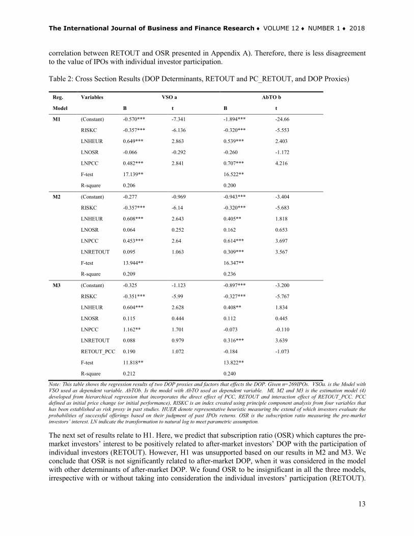
Hierarchical Regression Results Regression models presented in Table 2 consist of two dependent variables (AbTO and VSO) as proxies of after-market DOP. Findings reveal that all the models have good model fits, with high F-test values of 17.1 and 16.5 respectively, and p-values of less than 0.05, despite producing a low R-squares of 0.206 and 0.200 respectively. The first model (M1), using VSO as the dependent variable, has a slightly higher R-square as opposed to using AbTO as the dependent variable. The first model (M1) consists of a main independent variable (initial performance, defined as PCC, which surrogates for IPO underpricing) and three control variables. Findings show positive relationships between underpriced IPOs (PCC) and both proxies of after-market DOP (VSO and AbTO). The positive relationship between PCC and after-market DOP is a sign that investors update their beliefs differently leading to more disagreement of IPO value. The influence is stronger if market adjusted turnover (AbTO) is used, compared to offer turnover (VSO). Findings indicate that disagreement stimulates more trade for IPOs compared to the trade of other stocks in the capital market. Moving on to (H2) where participation of individual investors (RETOUT) is predicted to moderate the relationship between initial performance (PCC) and after-market DOP, we reject the null hypothesis based on findings relating to Models M2 and M3. The second regression model (M2) tests the direct influence of individual investors’ participation (RETOUT) on after-market DOP. The improvement of R-square (i.e. 0.236) when individual investors’ participation (RETOUT) is considered is evident if AbTO is assigned as a dependent variable. Findings also indicate that RETOUT plays an important role in explaining after-market DOP (captured by AbTO). However, the relationship between RETOUT and VSO was insignificant. Model M2 also indicates that RETOUT’s effect on AbTO is considered as indirect, as the direct effect reduces the influence of PCC on AbTO with a significant change in the R-square. Furthermore, the significant correlation between RETOUT and AbTO as well as the insignificant correlation between RETOUT and PCC (as in Appendix A) shows RETOUT to be a moderator in the relationship established between PCC and AbTO. Therefore, findings as in Model M3 indicate that RETOUT moderates the relationship between initial performance (PCC) and after-market DOP (captured by AbTO). When the moderating effect of RETOUT was considered in Model (M3), we found that the R-square of both proxies improve to 0.212 and 0.240 respectively. When AbTO is used as the dependent variable, the moderation effect of RETOUT subsumes the main effect of PCC on after-market DOP. The findings show that full moderation occurred, where the independent variable becomes insignificant, but the moderator is significant (Barron and Kenny, 1986, Aiken and West, 1991). The moderation effect is referred to as the buffering effect, in which the moderator (RETOUT) weakens the effect of the independent variable (PCC) on after-market DOP (see Frazier, Tix and Barron, 2004). On the other hand, when VSO was used as a dependent variable, the explanatory power of PCC increased. However, the result is inconclusive to support the moderation assumption, as RETOUT does not have a direct effect on after-market DOP as in Model 2. In hypothesizing on whether individual investors’ participation influence after-market investors’ choices, we found a significant and positive relationship between individual investors’ participation (RETOUT) and after-market DOP (AbTO). The result suggests that excessive trading in the after-market is not only among IPOs with greater risk compositions and underpriced IPOs, but also IPOs held by the less informed group. Findings suggest that participating individual investors take advantage of the after-market DOP to dispose their overpriced IPOs quickly. However, the negative regression coefficient of the interaction terms (PCC_RETOUT) when AbTO used as dependent variable, shows that after-market investors are not willing to pay a higher premium for the IPOs sold by the participating individual investors. Although it was previously maintained that individual investors receive more underpriced IPOs in Malaysia (see Jelic et al., 2001, How et al., 2007), the correlation results of our study show no evidence to support such a claim. Moreover, it was found that participating individual investors end up buying more undersubscribed IPOs (observed from the negative
The International Journal of Business and Finance Research ♦ VOLUME 12 ♦ NUMBER 1 ♦ 2018
13
correlation between RETOUT and OSR presented in Appendix A). Therefore, there is less disagreement to the value of IPOs with individual investor participation. Table 2: Cross Section Results (DOP Determinants, RETOUT and PC_RETOUT, and DOP Proxies)
Reg. Variables VSO a AbTO b
Model B t B t
M1 (Constant) -0.570*** -7.341 -1.894*** -24.66
RISKC -0.357*** -6.136 -0.320*** -5.553
LNHEUR 0.649*** 2.863 0.539*** 2.403
LNOSR -0.066 -0.292 -0.260 -1.172
LNPCC 0.482*** 2.841 0.707*** 4.216
F-test 17.139** 16.522**
R-square 0.206 0.200
M2 (Constant) -0.277 -0.969 -0.943*** -3.404
RISKC -0.357*** -6.14 -0.320*** -5.683
LNHEUR 0.608*** 2.643 0.405** 1.818
LNOSR 0.064 0.252 0.162 0.653
LNPCC 0.453*** 2.64 0.614*** 3.697
LNRETOUT 0.095 1.063 0.309*** 3.567
F-test 13.944** 16.347**
R-square 0.209 0.236
M3 (Constant) -0.325 -1.123 -0.897*** -3.200
RISKC -0.351*** -5.99 -0.327*** -5.767
LNHEUR 0.604*** 2.628 0.408** 1.834
LNOSR 0.115 0.444 0.112 0.445
LNPCC 1.162** 1.701 -0.073 -0.110
LNRETOUT 0.088 0.979 0.316*** 3.639
RETOUT_PCC 0.190 1.072 -0.184 -1.073
F-test 11.818** 13.822**
R-square 0.212 0.240
Note: This table shows the regression results of two DOP proxies and factors that effects the DOP. Given n=269IPOs. VSOa. is the Model with VSO used as dependent variable. AbTOb. Is the model with AbTO used as dependent variable. MI, M2 and M3 is the estimation model (4) developed from hierarchical regression that incorporates the direct effect of PCC, RETOUT and interaction effect of RETOUT_PCC. PCC defined as initial price change (or initial performance), RISKC is an index created using principle component analysis from four variables that has been established as risk proxy in past studies. HUER denote representative heuristic measuring the extend of which investors evaluate the probabilities of successful offerings based on their judgment of past IPOs returns. OSR is the subscription ratio measuring the pre-market investors’ interest. LN indicate the transformation to natural log to meet parametric assumption. The next set of results relate to H1. Here, we predict that subscription ratio (OSR) which captures the pre-market investors’ interest to be positively related to after-market investors’ DOP with the participation of individual investors (RETOUT). However, H1 was unsupported based on our results in M2 and M3. We conclude that OSR is not significantly related to after-market DOP, when it was considered in the model with other determinants of after-market DOP. We found OSR to be insignificant in all the three models, irrespective with or without taking into consideration the individual investors’ participation (RETOUT).

C. Narayanasamy et al | IJBFR ♦ Vol. 12 ♦ No. 1 ♦ 2018
14
Our findings are broadly consistent with those reported by Low and Yong (2013), Chong et al. (2009) and Chahine (2007) where subscription ratio is insignificant in justifying after-market divergence of opinion of fixed price IPOs. Overall, our results do not support the claim that unsuccessful individual investors (who could not subscribe the offers at time of offer in the primary market) will exhibit buying desire in the after-market or that investors’ attention in the pre-market influence opinions of after-market investors. Moving on, H3 predicts that the influence of representation heuristic on after-market DOP of IPOs is strengthened with individual investors’ participation. Our findings in Model M1 (Table 2) do not support H3. Findings suggest that investors’ opinion in the after-market is positively related to representative heuristic bias (HEUR), when both proxies of after-market DOP were utilized. The positive relationship between HEUR and after-market DOP is consistent with Bayley et al. (2006) but inconsistent with Chong et al. (2011). Representative heuristic bias seems to stimulate after-market trade. Meanwhile, after-market investors lack the capability to process market-wide information, particularly when degrees of uncertainty are high. Instead, they rely on the performance of past IPOs to make investment decisions. The high uncertainty is reflected by the inverse relationship between RISKC and after-market DOP proxies. The relationship suggests that smaller sized firms, smaller sized offers, less market capitalization, less reputable underwriters generate greater divergences of investors’ opinion in the after-market. However, when RETOUT was added to the model (M2) and when the moderation effect of RETOUT is considered in M3, the explanatory power of HEUR reduces but RISKC remains the same. These are indications that participating individual investors influence on after-market DOP is less affected by the representative heuristic bias. After-market investors’ belief that such offers lack recognition, hence pay less attention to the past success stories of individual investors’ trades, despite the evidence that the IPO participated by individual investors fare better in the future, than offers that generate higher first-day return. However, we do find that RISKC and HEUR play important roles in explaining after-market DOP of highly underpriced IPOs, while RETOUT plays an important role in explaining the after-market DOP of undersubscribed IPOs (of which are less underpriced). Model M1 in Table 3 shows the regression results for the two proxies of after-market DOP (VSO and AbTO), conditioned across hot issues and cold issues. Finding shows that that the F-test value of cold issues is higher if AbTO is used as dependent variable as compared VSO, indicates that the model using AbTO as a dependent variable have a good model fit, while the opposite holds for hot issues with a higher F-test value when VSO is used as dependent variable. Moving on to H5 with the prediction that hot IPOs with average initial performances greater than 10% significantly influence individual investors’ participation in IPOs with greater after-market divergence of opinion. However, the results in Model M2 of Table 3 do not support H5. When RETOUT was considered in Model M2, we found that RETOUT’s influence on VSO for cold and hot issues was insignificant. Nevertheless, the RETOUT’s influence on AbTO as in Model M2 was found to be significant for both cold and hot issue at 5% and 10% significance levels. Findings suggest that RETOUT plays an important role as a determinant of after-market DOP for both hot and cold issues, particularly for IPOs with turnover in excess of market turnover. The results in Model M1 shows that there is no significant relationship between PCC and after-market DOP proxies for hot issues. The results suggest there is no disagreement across hot issues. However, PCC was significantly positively related to after-market DOP for cold issues when AbTO was used as dependent variable. The PCC continue to be a significant determinant when AbTO is used as dependent variable, despite considering the effect of individual investors’ participation (RETOUT) for cold issues. Although participating individual investors dispose both hot and cold issues, hot issues were sold at a lower premium as indicated by the negative regression coefficient of PCC for hot issues. As for cold issues, less overpriced IPOs were sold giving support to the theory that investors hold on to losers for fear of regret (see Shefrin and Statman, 1985, Bayley at al., 2006, Barber and Odean, 1999, Barber and Odean,

The International Journal of Business and Finance Research ♦ VOLUME 12 ♦ NUMBER 1 ♦ 2018
15
2011, Chong, 2009). However, we do detect the presence of the cognitive bias called loss aversion in which after-market investors find more pleasure acquiring the winners at higher prices than acquiring losers at lower prices (see Kahneman and Tversky, 1979). However, these were not offers participated by individual investors. Findings relating to cold issue categorization suggest that disagreement occurs for less overpriced IPOs, and when individual investors’ participation was considered, the explanatory power reduces, indicating that less number of individual investors participated in these offers. Table 3: DOP Across Market Condition and the Effect of RETOUT
Reg. Variables VSOC a VSOH a AbTOC b AbTOH b.
Model t t t t
M1 (Constant) -0.884*** -6.248 -0.013 -0.113 -1.986*** -14.688 -1.365*** -11.413
RISK -0.359*** -3.771 -0.306*** -4.793 -0.381*** -4.181 -0.266*** -3.973
LNHEUR 0.869** 2.287 0.26 1.056 0.584* 1.607 0.103 0.399
LNOSR 0.808* 1.316 -0.320* -1.603 0.294 0.502 -0.290* -1.383
LNPCC 0.232 0.555 -0.101 -0.501 1.454*** 3.635 -0.141 -0.668
F-tests 6.616** 5.755** 9.216** 4.085**
R-square 0.168 0.151 0.22 0.112
M2 (Constant) -0.561 -1.157 0.328 1.049 -1.256*** -2.733 -0.623** -1.934
RISK -0.355*** -3.717 -0.303*** -4.747 -0.372*** -4.106 -0.259*** -3.946
LNHEUR 0.850** 2.225 0.212 0.851 0.539* 1.491 -0.001 -0.005
LNOSR 0.958* 1.469 -0.178 -0.764 0.632 1.024 0.019 0.079
LNPCC 0.066 0.136 -0.081 -0.401 1.077*** 2.354 -0.098 -0.47
LNRETOUT 0.112 0.696 0.114 1.17 0.252** 1.66 0.249*** 2.472
F-test 5.369** 4.891** 8.023** 4.620**
R-square 0.171 0.16 0.236 0.153
M3 (Constant) -0.403 -0.749 .826* 1.632 -1.366*** -2.682 -0.082 -0.156
RISK -0.359*** -3.743 -0.318*** -4.907 -0.369*** -4.057 -0.276*** -4.133
LNHEUR 0.818** 2.124 0.211 0.847 0.561* 1.536 -0.003 -0.012
LNOSR 1.004* 1.53 -0.216 -0.92 0.6 0.964 -0.022 -0.091
LNPCC 1.242 0.705 -1.397* -1.303 0.263 0.157 -1.528* -1.383
LNRETOUT 0.16 0.913 .257** 1.712 0.219* 1.317 0.403*** 2.613
RET_PCC 0.277 0.694 -0.374 -1.25 -0.192 -0.507 -0.407* -1.318
F-test 4.536** 4.354** 6.691** 4.161**
R-square 0.174 0.171 0.237 0.164
Note: This table shows the regression results of factors that effects DOP examined across hot and cold market condition. Given n (Hot IPOs) = 134; n (Cold IPOs) =135. VSOa. represents model with VSO as dependent variable. AbTOb represents model with AbTO as dependent variable. Model with VSO as dependent variable is categorized to VSOH for hot IPOs and VSOC for cold IPOs. Model with AbTO as dependent variable is categorized to AbTOC for cold IPOs and AbTOH for hot IPOs. MI, M2 and M3 is the estimation model developed from hierarchical regression that incorporates the direct effect of PCC, RETOUT and interaction effect of PCC_RETOUT. PCC defined as initial price change, RISKC is an index created using principle component analysis from four variables that has been established as risk proxy. HUER is a behavioral factor measuring the extent of which investors evaluate the probabilities of successful offerings based on their judgment of past IPOs return, or use of rule of thumb from past experience. OSR is the subscription ratio measuring the pre-market investor’s interest.
Model M3 in Table 3 shows that when the moderating effect of RETOUT is considered, the model fit improves as compared to Models M1 and M2 for both proxies of after-market DOP. The moderating

C. Narayanasamy et al | IJBFR ♦ Vol. 12 ♦ No. 1 ♦ 2018
16
effect improves the explanatory power of RETOUT and PCC on after-market DOP when both proxies were used as dependent variable, for hot issues. Nevertheless, based on the assumptions of Barron and Kenny (1986) and Aiken and West (1991), the moderating effect only occurs in cold issues when AbTO was used as a dependent variable, while partial moderation was observed for hot issues. For hot issues, significant positive relationships between PCC and both proxies of after-market DOP are observed if the interaction of PCC_RETOUT is incorporated into M3 Model. The positive regression coefficient of RETOUT suggests that participating individual investors dispose underpriced IPOs at a lower premium for fear of regret, while the negative regression coefficient is a sign that less underpriced and undersubscribed IPOs are disposed on the first-day of trade by participating individual investors. One interpretation is that the participating individual investors quickly dispose the less underpriced IPOs and hold on to the overpriced IPOs, losses is seen to induce more pain than pleasure resulting from the gain called loss aversion. Meanwhile, after-market investors demand lower premiums (during the hot period) from the participating individual investors for the lack of quality recognition of such offers. Our results across hot and cold issue IPOs are consistent with the findings by Krigman et al. (1999) and Gounopolous (2006) where extremely hot issues are traded less while cold issues are traded more. The findings for hot issue is inconsistent with the findings by Aggarwal (2003), Bayley et al. (2006) and Low and Yong (2013) perhaps due to the rise of the volume movement in the after-market from as low as 7% (see Chong et al., 2009) to an average of 101.8% in our study, while the changes in the initial performance remain low. The large trade is accounted for by the sale of undersubscribed and less underpriced IPOs by participating individual investors, while highly underpriced IPOs which are subscribed by more informed groups are possibly not disposed early.
To summarize, the findings show that RETOUT plays a positive role on volume behavior, particularly when there is greater disagreement in the after-market. Upon further investigation, it was found that individual investors’ participation (RETOUT) have a significant moderating role on the relationship between initial performance PCC and after-market DOP for cold issues and hot issues. The explanatory power of hot issues is greater than that for cold issues. Other determinants considered in our study include the heuristic representation (HEUR) and risk composition (RISKC). Both show significant influences on after-market DOP. Our study offers a new insight to the role of individual investors’ participation on after-market activity. Their participation points to behavioral forces at work in the after-market for less underpriced and undersubscribed share issues. After-market investors’ decision to purchase such IPOs at lower premiums seem to be suboptimal decisions, as they do not result in favorable future returns. On the other hand, participating individual investors’ decision to dispose less underpriced IPOs is seen to be optimal, while the decision to dispose less overpriced IPOs is a sign of loss aversion, in which investors find that the pain from realizing losses is greater than the pleasure derived from gains. CONCLUSION We conducted an investigation of after-market divergence of opinion (DOP) and its relation to initial performance (PCC which surrogates underpriced IPOs), individual investors’ participation (RETOUT), risk factors (RISKC), representative heuristic bias (HEUR) and post-IPO performance (AMAR). There is a significant positive relationship between individual investors’ participation and after-market DOP in the Malaysian IPO market. We also found that after-market DOP attributes to a negative correlation with post IPO performance, while initial performance (PCC) and RETOUT have positive correlations with post-IPO performance. Overall our regression results across different market conditions suggest that after-market investors are not willing to pay higher prices for the offers originally held by individual investors, while original individual subscribers are willing to forgo their underpriced IPOs at a low premium for fear of regret of holding such shares for longer period (aversion to losses, in which the pain from uncurring losses is believed to be more severe as compared to the pleasure derived from gains, as per the prediction by Kahneman and Tversky, 1979). This is also partly due to the widespread belief that institutions are ‘recognized’ measures of firm quality (see Boehme and Colak, 2012), while retail investors are not

The International Journal of Business and Finance Research ♦ VOLUME 12 ♦ NUMBER 1 ♦ 2018
17
accorded such recognition. The belief held by the after-market investors is often to the advantage of institutional investors, but at the expense of retail investors (see Barber and Odean, 2011). Even though offers with individual investors’ participation were found to perform better in the long-run (consistent with Bayley et al.,2006), after-market investors place lower values for such IPOs, therefore, most individual investors who subscribe to undersubscribed IPOs are willing to forgo their holding fast at a lower premium. We found that the total number of individual investors participating in Malaysian IPOs is relatively small. Findings indicate that only 34% of IPO shares offered (or, 4.4% of total outstanding shares) is subscribed by individual investors. Most of these issues are largely undersubscribed and overpriced. These findings are at odds with past studies who found that underpriced IPOs in Malaysia are largely held by individual investors (Jelic et al., 2001, How et al., 2007). Although behavioral forces such as heuristic representation, loss aversion and divergence of opinion exist in the Malaysian market, the effects of such forces are weak. In terms of policy implications, the liquidity of retail sales in both hot issue and cold issue periods should be improved by market regulators, perhaps by increasing the proportion of underpriced shares offered to individual investors. Second, there is a need to review the current IPO pricing method, as both the pre-market and after-market individual investors face difficulties in ascertaining the values of the said IPOs. Such offers should be offered in an institutional setting, to ensure that behavioral forces remain low and retail investors do not lose from their own trading activity. Third, since risk composition factors significantly influence after-market investors’ opinion, there is a need to further scrutinize each component that collectively make up the risk composition element. For instance, the liberalization of underwriters’ requirement for new share offerings in Malaysia would likely make it more difficult for individual investors in terms of ascertaining the value of new shares. Therefore, there is a need revise the role of underwriters instead of merely removing the underwriter requirement for new share offerings. One of the main limitations of our paper is that, despite having included all recent IPOs carried out in the Malaysian stock exchange, the size of our sample remains relatively small as compared to other IPO-centered studies undertaken in more advanced capital markets such as the US and the UK. In addition, we did not make the distinction between the different listing boards where IPO firms eventually feature (i.e, Main Board, Second Board, MESDAQ, Main Market or ACE markets). These drawbacks may limit the generalizability of our findings to other developing capital markets. Hence, in terms of suggestions for future research, our study should be extended by considering IPOs across all major markets in the Southeast Asian region or, more broadly, the East Asian region. This would greatly increase the overall sample size for statistical analysis. Second, we have not taken into account other potentially relevant factors such as corporate governance where the quality of disclosures made in IPO prospectuses may have some impact on the investors pre-market interest (i.e subscription ratio). Lastly, a comparative study across markets where individual investor participation form significant proportion of overall trading volume may also be fruitful in terms of providing insights into the impact of their trading activities on the DOP phenomenon.

C. Narayanasamy et al | IJBFR ♦ Vol. 12 ♦ No. 1 ♦ 2018
18
APPENDIX Appendix A: Correlations of Dependent and Independent Variables
LNVSO LNAbTO LNAMAR LNOSR LNHEUR RISK LNRETOUT LNPCC
LNVSO 1 0.831** -0.154** 0.213** 0.208** -0.359** 0.01 0.246**
LNAbTO 1 -0.156** 0.174** 0.192** -0.318** 0.155* 0.297**
LNAMAR 1 0.032 -0.064 0.009 0.036 0.412**
LNOSR 1 0.272** -0.338** -0.444** 0.343**
LNHEUR 1 0.017 0.048 0.282**
RISK 1 0.160** -0.130*
LNRETOUT 1 0.007
LNPCC 1
Note. 289IPOs. VSO denotes the total volume of trade at first-day scaled by shares offered. AbTO measures the market adjusted turnover at first-day of trade. AMAR measures the one-year post IPO returns. RETOUT denotes retail shares scaled by outstanding shares. PCC denotes initial price change measured as the deviation of closing price at first-day of trade scaled by offer price. OSR is the subscription ratio measuring the pre-market investor’s interest. HEUR denotes representative heuristic bias measuring the extend of which investors evaluate the probabilities of successful offerings based on the their judgment of past IPO returns. RISK defines risk composition index formed using principle component analysis upon removing OSIZE and AGE with correlation > 0.9 and <0.3 **. LN represents the natural logarithm transformation of the respective variable to meet the assumptions underlying least-square estimator. Correlation is significant at the 0.01 level (2-tailed). * Correlation is significant at the 0.05 level (2-tailed). REFERENCES Aggarwal, R. (2003) “Allocation of initail public offering and flipping activity,” Journal of Financial Economics, Vol. 68, p. 111-135. Aggarwal, R., Prabhala, N. R. and Puri, M. (2002) “Institutional allocation in initial public offerings: Empirical evidence,” The Journal of Finance, Vol. 57(3), p. 1421-1442. Ahmad-Zaluki, N. A. and Lim, B. K. (2012) “The investment performance of Mesdaq Market initial public offerings,” Asian Academy of Management Journal of Accounting and Finance, Vol. 8(1), p. 1–23. Aiken, L. S. and West, S. G. (1991) Multiple Regression Testing and Interpreting Interactions. New Bury Park California: Sage Publication Inc. A´lvarez, S. and Gonza´lez, V. M. (2005) “Signaling and the long-run performance of Spanish initial public offerings (IPOs),” Journal of Business Finance & Accounting, Vol. 32(1 & 2), p. 325-350. Barber, B. M. and Odean, T. (2011) “The behavior of individual investors,” Retrieved September 25, 2015, from http://ssrn.com/abstract=1872211. Barber, B. M. and Odean, T. (1999) “The courage of misguided convictions,” Financial Analyst Journal, Vol. 55(6), p. 41–55. Barron, R, N. and Kenny, D. A. (1986) “The moderator–mediator variable distinction in social psychological research: Conceptual, strategic and statistical considerations,” Journal of Personality and Social Psychology, Vol. 51(6), p. 1173-1182. Bayley, L., Lee, J. P. and Walter, T. S. (2006) “IPO flipping in Australia: Cross sectional explanations,” Pacific Basin Finance Journal, Vol. 14, p. 327-348.

The International Journal of Business and Finance Research ♦ VOLUME 12 ♦ NUMBER 1 ♦ 2018
19
Boehme, R. and Çolak, G. (2012) “Primary market characteristics and secondary market frictions of stocks,” Journal of Financial Markets, Vol. 15(2), p. 286-327. Brav, A. and Heaton, J., B. (2002) “Competing theories of financial anomalies,” The Review of Financial Studies, Vol. 15(2), p. 575-606. Chahine, S. (2007) “Investor interest, trading volume, and the choice of IPO mechanism in France,” International Review of Financial Analysis, Vol. 16(2), p. 116-135. Chen, Hsuan-Chi and Guo, Wen-Chung. (2010) “Divergence of opinion and initial public offerings,” Review of Quantitative Finance and Accounting, Vol. 34(1), p. 59-79. Chong, F. (2009) “Disposition Effect and Flippers in the Bursa Malaysia,” The Journal of Behavioral Finance, Vol. 10, p. 152–157. Chong, N. F., Ali, R. and Ahmad, Z. (2009) “Does noise signal affect flipping activities,” International Journal of Banking and Finance, Vol. 6(2), p. 111-127. Chong, F. N., Ahmad, Z and Ali, R. (2011) “Representative heuristic and the after-market dynamics of the new listing in Malaysia,” Labuan Bulletin of International Busines and Finance, Vol. 9, p. 1-11. Chowdhry, B., and Nanda, V. (1996) “Stabilization, syndication, and pricing of IPOs,” Journal of Financial and Quantitative Analysis, Vol. 31(1), p. 25-42. Dhar, R., and Zhu, N. (2006) “Up close and personal: Investor sophistication and the disposition effect,” Management Science, Vol. 52(5), p. 726-740. Dawson, S. M. (1987) “Secondry stock market performance of initial public offering in Hong Kong, Singapore and Malaysia: 1978-1984,” Journal of Business Finance & Accounting, Vol. 14(1), p. 65-76. Diether, K. B., Malloy, C.J. and Scherbina, A. (2002) “Differences of opinion and the cross-section of stock returns,” The Journal of Finance, Vol. 57(5), p. 2113-2141. Ellis, K. (2006) “Who trades IPOs? A close look at the first days of trading,” Journal of Financial Economics, Vol. 79, p. 339-363. Fama, E. F. (1998) “Market efficiency, long-term returns, and behavioral finance,” Journal of Financial Economics, Vol. 49(3), p. 283–306. Frazier, P. A., Tix, A. P. and Barron, K. E. (2004) “Testing moderator and mediator effects in counselling psychology research,” Journal of Counselling Psychology, Vol. 51(1), p. 115–134. Gao, Y., Mao, C. X. and Zhong, R. (2006) “Divergence of opinion and long-run performance of initial public offering,” Journal of Financial Research, Vol. 29(1), p. 113-129. Garfinkel, J. A. (2009) “Measuring investors' opinion divergence,” Journal of Accounting Research, Vol. 47(5), p. 1317-1348. Goetzmann, W. N. and Massa, M. (2005) “Dispersion of opinion and stock returns,” Journal of Financial Markets, Vol. 8(3), p. 324-349.

C. Narayanasamy et al | IJBFR ♦ Vol. 12 ♦ No. 1 ♦ 2018
20
Gounopoulos, D. (2006) Flipping Activity in Fixed Offer Price mechanism allocated IPO’s. Elsevier Butterworth, Heinemann, Burlington, pp. 159-175. Harris, M. and Raviv, A. (1993) “Differences of opinion make a horse race,” Review of Financial Studies, Vol. 6(3), p. 473-506. Hong, H. and Stein, J. C. (2007) “Disagreement and the stock market,” Journal of Economic Perspectives, Vol 21(2), p. 109-128. Houge, T., Loughran, T., Yan, X. S. and Suchanek, G. (2001) “Divergence of opinion, uncertainty, and the quality of initial public offerings,” Financial Management, Vol. 30(4), p. 5-23. How, J., Jelic, R., Saadouni, B. and Verhoeven, P. (2007) “Share allocations and performance of KLSE second board IPOs,” Pacific-Basin Finance Journal, Vol. 15(3), p. 292-314. Ibbotson, R. G. and Jaffe, J. F. (1975) “Hot issue markets,” The Journal of Finance, Vol. 30(4), p. 1027-1042. Jelic, R., Saadouni, B. and Briston, R. (2001) “Performance of Malaysian IPOs: Underwriters reputation and management earnings forecasts,” Pacific-Basin Finance Journal, Vol. 9(5), p. 457-486. Jewartowski, T. and Lizińska, J. (2012) “Short and long-term performance of Polish IPOs,” Emerging Markets Finance & Trade, Vol. 48(2), p. 59-75. Kahneman, D. and Tversky, A. (1973) “On the psychology of prediction,” Psychological Review, Vol. 80-84, p. 237-251. Kahneman, D. and Tversky, A. (1979) “Prospect theory: An analysis of decsison under risk,” Econometrica, Vol. 47(2), p. 263-291. Kahneman, D. and Tversky, A. (1982) Intuitive Predictions: Biases and Corrective Procedures. Judgment under Uncertainty: Heuristics and Biases. England: Cambridge University Press. Kandel, E. and Pearson, N. D. (1995) “Differential interpretation of public signals and trade in speculative markets,” Journal of Political Economy, Vol. 103(4), p. 831-872. Karpoff, J. M. (1986) “A theory of trading volume,” The Journal of Finance, Vol. 41(5), p. 1069-1087. Kaustia, M. (2004) “Market-wide impact of the disposition effect: Evidence from IPO trading volume,” Journal of Financial Markets, Vol. 7, p. 207– 235. Krigman, L. Shaw, H. W and Womack, K.L. (1999) “The persistence of IPO mispricing and the predictive power of flipping,” The Journal of Finance, Vol. 54(3), p. 1015-1044. Loughran, T. and Ritter, J. (2004) “Why has IPO underpricing changed over time?,” Financial Management, p. 5-37. Low, S. W. and Yong, O. (2013) “Initail public offering and investor heterogeneity: evidence from Malaysia,” American Journal of Finance and Accounting, Vol. 3(1), p. 41-56.

The International Journal of Business and Finance Research ♦ VOLUME 12 ♦ NUMBER 1 ♦ 2018
21
Miller, E. M. (1977) “Risk, uncertainty, and divergence of opinion,” The Journal of Finance, Vol. 32(4), p. 1151-1168. Miller, R. E. (2000) “Long-run Underperformance of initial public offerings: An explanation,” Working Paper no. 1999-18, Department of Economics and Finance, University of New Orleans. Miller, R. E. and Reilly, F. K. (1987) “An examination of mispricing, returns and uncertainty for initial public offerings,” Financial Management, Vol. 16(2), p. 33-38. Moshirian, F., Ng, D. and Wu, E. (2010) “Model specification and IPO performance: New insights from Asia,” Research in International Business and Finance, Vol. 24(1), p. 62-74. Odean, T (1998) “Are investors reluctant to realize their losses,” The Journal of Finance, Vol. 53(5), p. 1775-1798. Paudyal, K., Saadouni, B. and Briston, R. J. (1998) “Privatization initial public offerings in Malaysia: Initial premium and long-term performance,” Pacific-Basin Finance Journal, Vol. 6(5), p. 427-451. Ritter, J. R. (1984) “The hot Issue market of 1980,” The Journal of Business, Vol. 57(2), p. 215-240. Ritter, J., R. (1991) “The long-run performance of initial public offering,” The Journal of Finance, Vol. 46 (1), p. 1-27. Rock, K. (1986) “Why new issues are underpriced. Journal of Financial Economics,” Vol. 15(1&2), p. 187-212. Shalen, C. T. (1993) “Volume, volatility, and the dispersion of beliefs,” The Review of Financial Studies, Vol. 6(2), p. 405-434. Shefrin, H. and Statman, M. (1985) “The disposition to sell winners too early and ride losers too long,” The Journal of Finance, Vol. 40(3), p. 777-790. Tversky, A. and Kahneman, D. (1974) “Judgment under uncertainty heuristic and bias,” Science, p. 1124-1131. Wang, H and Liu, X. (2014) “The impact of investor heterogeneity in beliefs on share repurchase,” International Journal of Econometrics and Financial Management, Vol. 2(3), p. 102-113. Yong, O. (2007) “A review of IPO research in Asia: What's next?,” Pacific-Basin Finance Journal, Vol. 15(3), p. 253-275. Yong, O. (2010) “Initial premium, flipping activity and opening-day price spread of Malaysian IPOs,” Capital Market Review, Vol. 18(1&2), p. 45-6. BIOGRAPHY
Dr. Cheedradevi Narayanasamy is currently the Head of Accounting and Finance Department at Nilai University, Malaysia. She holds Bachelors of Accountancy (Hons) from University Putra Malaysia, MBA in Applied Finance and Investment and Ph.D in Finance from National University of Malaysia. Previously she served as a senior lecturer within a leading private higher education industry (UTAR), Malaysia. The author has wide teaching experience and has presented academic papers in international

C. Narayanasamy et al | IJBFR ♦ Vol. 12 ♦ No. 1 ♦ 2018
22
conferences, and published articles in a number of peer review journals. The author holds a Staff Education and Development Association (SEDA) teaching award from United Kingdom. She has also been a reviewer for Pearson International Inc. She can be reached at [email protected] or [email protected]. Prof. Dr. Izani Ibrahim is a finance professor currently attached to College of Business, Prince Sultan University, Riyadh. Prior to joining PSU, he held the role as the Dean for Graduate School of Business, National University of Malaysia. He is well known for his research, teaching and supervisory experience in the field of finance and time series analysis. Prof Dr. Izani has published in highly reputable finance and economic journals. He can be reached at [email protected] or [email protected] Dr. Yeoh Ken Kyid is an Assistant Professor of CSR, Ethics & Governance at Nottingham University Business School (Malaysia Campus). He is also a Fellow of the UK’s Higher Education Academy. Prior to joining NUBS, he held the role of Associate Dean for Research & Innovation at Taylor’s Business School, Taylor’s University. In addition, he taught for seven years at Newcastle Business School, Northumbria University in the United Kingdom. Ken has published papers in highly regarded journals (e.g. Industrial Management & Data Systems, The Journal of Developing Areas, etc.) besides regularly presenting papers at international academic conferences. Ken is also a recipient of the prestigious Newton Advanced Fellowship that is jointly funded by The British Academy and Academy of Sciences Malaysia. He has also delivered guest lectures at Hong Kong Polytechnic University, City University of Hong Kong and De Montfort University (UK) in the past. He can be reached at [email protected]

The International Journal of Business and Finance Research Vol. 12, No. 1, 2018, pp. 23-38 ISSN: 1931-0269 (print) ISSN: 2157-0698 (online)
www.theIBFR.com
23
THE EFFECT OF REAL EXCHANGE RATE
VOLATILITY ON EXPORTS IN THE BALTIC REGION Carlos Moslares, Universitat Ramon Llull, Spain E. M. Ekanayake, Bethune-Cookman University
ABSTRACT
In this paper we analyze the effects of the real exchange rate volatility on exports in the Baltic region. The study focuses on three countries in the Baltic region, namely, Estonia, Latvia, and Lithuania, and uses quarterly exports of these countries to their major trading partners over the period from 1993Q1 to 2014Q4. It uses both the panel co-integration analysis and the method of bounds testing or the Autoregressive Distributed Lag (ARDL) approach to co-integration analysis to estimate the short-run and long-run effects of the real exchange rate volatility on exports. Our results reveal that exports depend positively on the levels of foreign economic activity but negatively on relative prices and real exchange rate. However, the exchange rate volatility tends to provide mixed effects. Furthermore, the effects of exchange volatility are found to yield mixed effects both in the short-run and the long-run. The results also indicate that the effects vary from country to country. JEL: F14, F31 KEYWORDS: Baltic Countries, Exports, Exchange Rate Volatility, GARCH Volatility Measures, Panel
Unit Roots, Panel Co-integration INTRODUCTION
here are numerous theoretical and empirical studies that analyze the effects of the exchange rate volatility on international trade flows. Notwithstanding the sizeable number of studies conducted, no real consensus about the impact of exchange rate volatility on trade has emerged. Most of the
empirical studies have found that exchange rate volatility tends to reduce the level of trade. Some of these studies include, Byrne, Darby, and MacDonald (2008), Choudhry (2005), Bahmanee-Oskooee (2002), Arize, et al. (2000), Arize (1995), Chowdhury (1993), Pozo (1992), and Bahmani-Oskooee and Ltaifa (1992). Some of the reasons for a negative relationship between exchange rate volatility and trade flows include (a) exchange rate volatility may affect exports directly through uncertainty and adjustment costs for risk-averse exporting investors, and (b) exchange rate volatility may have an indirect effect through its impact on the structure of output, investment and government policy. Some empirical studies have found a positive relationship or an insignificant negative relationship between exchange rate volatility and trade flows. Examples of such studies include Doyle (2001), Chou (2000), McKenzie and Brooks (1997), Qian and Varangis (1994), Kroner and Lastrapes (1993), Assery and Peel (1991), Aristotelous (2001), Bahmani-Oskooee and Payestch (1993), Bahmani-Oskooee (1991), and Hooper and Kohlhagen (1978). Exchange rate volatility making exporting more attractive to risk-tolerant exporting firms has often been cited as the plausible reason for a positive relationship between the two variables. There are several reasons for contradictory results by different studies. Some of the reasons include: the differences in the measurement of exchange rate volatility; the differences in type of sample data used, for example, the use of aggregate export data versus sectoral export data; the differences in time-frames; and the differences in econometric methods used. With better access to sectoral data combined with the
T

C. Moslares & E. M. Ekanayake | IJBFR ♦ Vol. 12 ♦ No. 1 ♦ 2018
24
development of more sophisticated econometric models, recent studies have begun evaluating the exchange rate volatility-export connection from a sectoral perspective. The results of the studies that make use of sectoral data may be more revealing than aggregate studies given that different trade sectors would be impacted differentially by exchange rate volatility. This study focuses on export flows from each of the three countries selected (Estonia, Latvia, and Lithuania) to its top 20 exports destinations to uncover the nature and sensitivity of the relationship between exchange rate volatility and exports. In each country, the top 20 export destinations selected account about 90% of its total exports to the world. We use both the panel co-integration and the method of bounds testing or the Autoregressive Distributed Lag (ARDL) approach to co-integration analyses for this purpose. Using these approaches we investigate the effects of exchange rate volatility on exports over a period of 22 years using quarterly data from 1993Q1 to 2014Q4. The paper is organized as follows: We provide a brief review of the literature in Section 2. Thereafter, in Section 3 we lay the empirical framework of our study by specifying our model. In Section 4 we discuss variable definitions and outline our data sources. Empirical results from the panel co-integration, bounds testing approach to co-integration, and error-correction model estimates are presented in Section 5. The final section presents a summary and conclusion of the results obtained in this study. LITERATURE REVIEW In this section we present a brief overview of studies that examine the exchange rate volatility-trade nexus. We begin by discussing the most recent and sophisticated studies, employing co-integration techniques and error-correction models, to older, less complex studies. For a comprehensive review of empirical studies, see Bahmani-Oskooee and Hegerty (2007). Bahmani-Oskooee and Harvey (2011) investigate the effects of exchange rate fluctuations on trade flows between the U.S. and Malaysia using disaggregated, industry-level annual export and import data for 17 export industries and 101 importing industries from 1971 to 2006. They conclude that while exchange rate volatility exerts short-run effects in trade flows of almost two-thirds of the industries, these effects last into the long-run in 38 U.S. exporting industries and in 10 U.S. importing industries. Bahmani-Oskooee and Hegerty (2009) investigate the effects of exchange rate fluctuations on trade flows between the U.S. and Mexico using disaggregated, industry-level annual export and import data for 102 industries from 1962 to 2004. They analyze both the short- and long-term effects of volatility in the peso/dollar real exchange rate on Mexican-United States trade. They conclude that in the short-term increased volatility negatively affects trade flows in most industries. Long-term effects however, are significant for only one-third of the industries studied, and of this, only two-thirds are negative. They speculate that increased Mexican integration and liberalization of economic policies allow for greater adjustments in the long-term so that volatility is less of a problem in the long-term than in the short-term. Byrne, Darby, and MacDonald (2008) analyze the impact of exchange rate volatility on the volume of bilateral U.S. trade flows using homogenized and differentiated sectoral annual data over the period 1989-2001 for a cross-section of 6 EU countries and 22 industries. Their study finds that clustering all industries together provides evidence of a negative effect on trade from exchange rate volatility, which confirms findings of other studies using aggregate data. However, when investigating sectoral trade differences, the effects of exchange rate volatility on trade is negative and significant for differentiated goods and insignificant for homogeneous goods, confirming recent studies that sectoral differences are in fact crucial to explaining the differential impact of volatility on trade. They suggest that a greater degree of disaggregation at the industry level may provide more worthwhile results, which is what we do in this study. Bahmani-Oskooee and Kovyryalova (2008) investigate the effect of exchange rate fluctuations on trade flows between the U.S. and the United Kingdom using disaggregrated annual export and import data for 177 commodities industries from 1971 to 2003. They analyze both the short- and long-term effects of real exchange rate volatility on trade between the U.S. and the UK. Their results reveal that the volatility

The International Journal of Business and Finance Research ♦ VOLUME 12 ♦ NUMBER 1 ♦ 2018
25
of the real dollar–pound rate has a short-term significant effect on imports of 109 industries and on exports of 99 industries. In most cases, such effects are unfavorable. In the long run, however, the number of significant cases is somewhat reduced: only 62 import and 86 export industries are significantly and adversely affected by exchange rate volatility. The industries affected involve both durable and non-durable goods, and include small as well as large industries, supporting findings by aggregate studies. In another study, Bahmani-Oskooee and Mitra (2008), investigate the effects of exchange rate volatility on trade flows between the U.S. and India, an emerging economy. Using annual data from 40 industries from 1962–2004, their results demonstrate that exchange rate volatility has more short-run than long-run effects. In the short-run, 17 industries were affected on the import side and 15 on the export side. The industries affected show India’s increasing ability to produce import substitutable goods. However, in the long run, only a few industries are affected because the increasing dependence on trade between India and the US cause industries to respond inelastically to exchange rate volatility. Using both the nominal and the real exchange rate between the United States dollar and the currencies of Canada and Japan, Choudhury (2005) investigates the influence of exchange rate volatility on U.S. real exports to Canada and Japan using aggregate monthly data ranging from January 1974 to December 1998. The study uses conditional variance from the GARCH (1, 1) model as a measure of exchange rate volatility, and finds significant and mostly negative effects of exchange rate volatility on real exports. As in the above studies, Sukar and Hassan (2001) investigate the relationship between U.S. trade volume and exchange rate volatility using co-integration and error-correction models. Their study uses quarterly aggregate data covering the period 1975Q1 – 1993Q2 and a GARCH model to measure the exchange rate volatility. Paralleling other studies, the authors find evidence for a significantly negative relationship between U.S. export volume and exchange rate volatility. However, unlike other findings, they reveal that the short-run dynamics of the exchange rate volatility -trade relationship is insignificant. They argue that this result may be due to the existence of avenues for hedging against exchange risks so as to neutralize the negative impact of exchange rate volatility. Other scholars argue that this short-run insignificant relationship may be because of the investigators’ use of aggregate data, which ignores sectoral differences. For example, while one sector may exhibit a negative relationship, another may exhibit an equal but opposite effect so that they offset each other. Finally, Arize (1995), using monthly series from February 1978 to June 1986 analyzes the effects of real exchange rate volatility on the proportions of bilateral exports of nine categories of goods from the U.S. to seven major industrial countries. The volatility measure employed is the standard deviation of the monthly percentage change in the bilateral exchange rate between the U.S. and the importing country from t to t-12. The study reveals differential effects of exchange rate volatility across different categories of exports. The study also concludes that exchange rate uncertainty has a negative effect on U.S. real exports, and that it may have a major impact on the allocation of resources to different industries depending on trade elasticities. One major problem with most of the studies above is that the sample period includes the period prior to the end of the fixed exchange regime, so results may include the lag effects of fixed exchange rates on trade before 1973 lingering on during the transition period after the implementation of the floating exchange rate regime. The current study corrects for this potential bias by using quarterly exports data covering a 22-year period from 1993Q1 to 2014Q4. The methodology used in this study incorporates the recent developments in the literature, namely, the panel co-integration method and the ARDL approach to co-integration analysis, which may uncover the nature and sensitivity of the real exchange rate volatility-exports nexus.

C. Moslares & E. M. Ekanayake | IJBFR ♦ Vol. 12 ♦ No. 1 ♦ 2018
26
METHODOLOGY Model Specification The objective of this study is to assess the effects of exchange rate volatility on exports. The study uses quarterly exports data of three countries in the Balkan region, namely, Estonia, Latvia, and Lithuania. For each country, quarterly exports data for top 20 export destinations were selected. Drawing on the existing empirical literature, we specify that a standard long-run reduced-form export demand function to take the following functional form (see, for example, Pino, Das and Sharma, 2016; Ozturk and Kalyonku, 2009; Choudhry, 2005; Arize, 1998, 1996, 1995; and Asseery and Peel, 1991): ln𝑋𝑋𝑡𝑡 = 𝛽𝛽0 + 𝛽𝛽1𝑇𝑇𝑇𝑇𝑇𝑇𝑇𝑇𝑇𝑇 + 𝛽𝛽2𝑙𝑙𝑇𝑇𝑌𝑌𝑡𝑡 + 𝛽𝛽3𝑙𝑙𝑇𝑇𝑃𝑃𝑡𝑡 + 𝛽𝛽4𝑙𝑙𝑇𝑇𝑉𝑉𝑡𝑡 + 𝛽𝛽5𝑙𝑙𝑇𝑇𝑅𝑅𝑅𝑅𝑅𝑅𝑡𝑡 + 𝜀𝜀𝑡𝑡 (1) where Xt is the real export volume in period t, Trend represents the linear trend, Yt is the real foreign income in period t, Pt is the relative price of exports in period t, Vt is a measure of exchange rate volatility, RERt is the real exchange rate in period t, and εt is a white-noise disturbance term. Economic theory posits that the real income level of the domestic country’s trading partners would have a positive effect on the demand for its exports. Therefore, a priori, we would expect that β2 > 0. On the other hand, if the relative price of exports rise (fall), domestic goods become less (more) competitive than foreign goods, causing the demand for exports to fall (rise). Therefore, a priori, one would expect that β3, which measures the competitiveness of a given Balkan country’s exports relative to trading partner’s domestic production, is negative. The third explanatory variable is a measure of exchange rate volatility. Various measures of real VOL have been proposed in the literature. Some of these measures include (1) the averages of absolute changes, (2) the standard deviations of the series, (3) the deviations from the trend, (4) the squared residuals from the ARIMA or ARCH or GARCH processes, and (5) the moving sample standard deviation of the growth rate of the real exchange rate. In this study, two alternative measures of exchange rate volatility were used. Since the effects of V on exports have been found to be empirically and theoretically ambiguous (Bredin, et al. 2003), β4 could be either positive or negative. An increase (a decrease) in real exchange rate indicates an appreciation (a depreciation) of the domestic currency which depresses (boosts) exports. Therefore, a priori, one would expect that β5 to be negative. Equation (1) shows the long-run relationships among the dependent and independent variables in our model. Given the recent advances in time-series analysis, in estimating the long-run model outlined by equation (1), it is now a common practice to distinguish the short-run effects from the long-run effects. For this purpose, equation (1) should be specified in an error-correction modeling (ECM) format. This method had been used in many recent studies including Pino, Tas and Sharma (2016), Bahmani-Oskooee and Hegerty (2009), Bahmani-Oskooee and Wang (2008, 2009), Bahmani-Oskooee and Mitra (2008), Bahmani-Oskooee and Kovyryalova (2008), and Bahmani-Oskooee and Ardalani (2006). According to Bahmani-Oskooee and Wang (2008), such an approach is warranted given that the measure of exchange rate volatility is a stationary variable (see, for example, De Vita and Abbot, 2004; Bahmani-Oskooee & Payesteh, 1993; and Doyle, 2001), whereas the other variables in equation (1) could be non-stationary. Therefore, following Pesaran, Shin, and Smith (2001) and their method of bounds testing or the Autoregressive Distributed Lag (ARDL) approach to co-integration analysis, we rewrite equation (1) as an ARDL-ECM model in equation (2) below. ∆𝑙𝑙𝑇𝑇𝑋𝑋𝑡𝑡 = 𝜌𝜌0 + 𝜌𝜌1𝑇𝑇𝑇𝑇𝑇𝑇𝑇𝑇𝑇𝑇 + ∑ 𝑎𝑎𝑖𝑖∆𝑙𝑙𝑇𝑇𝑋𝑋𝑡𝑡−𝑖𝑖𝑛𝑛
𝑖𝑖=1 + ∑ 𝑏𝑏𝑖𝑖∆𝑙𝑙𝑇𝑇𝑌𝑌𝑡𝑡−𝑖𝑖𝑛𝑛𝑖𝑖=0 + ∑ 𝑐𝑐𝑖𝑖∆𝑙𝑙𝑇𝑇𝑃𝑃𝑡𝑡−𝑖𝑖𝑛𝑛
𝑖𝑖=0 +∑ 𝑇𝑇𝑖𝑖∆𝑙𝑙𝑇𝑇𝑉𝑉𝑡𝑡−𝑖𝑖𝑛𝑛𝑖𝑖=0 +
∑ 𝑇𝑇𝑖𝑖∆𝑙𝑙𝑇𝑇𝑅𝑅𝑅𝑅𝑅𝑅𝑡𝑡−𝑖𝑖𝑛𝑛𝑖𝑖=0 + 𝜋𝜋0𝑋𝑋𝑡𝑡−1 + 𝜋𝜋1𝑌𝑌𝑡𝑡−1 + 𝜋𝜋2𝑃𝑃𝑡𝑡−1 + 𝜋𝜋3𝑉𝑉𝑡𝑡−1 + 𝜋𝜋4𝑅𝑅𝑅𝑅𝑅𝑅𝑡𝑡−1 + 𝜖𝜖𝑡𝑡 (2)
where Δ is the difference operator and the other variables are as defined earlier, n is the lag length, and ϵt is a random error term. Pesaran, Shin, and Smith’s (2001) bounds testing approach to cointegration is

The International Journal of Business and Finance Research ♦ VOLUME 12 ♦ NUMBER 1 ♦ 2018
27
based on two procedural steps. The first step involves using an F-test or Wald test to test for joint significance of the no cointegration hypothesis Ho: π0 = π1 = π2 = π3 = π4 = 0 against an alternative hypothesis of cointegration, H1: π0 ≠ 0, π1 ≠ 0, π2 ≠ 0, π3 ≠ 0, π4 ≠ 0. This test is performed using equation (2). The advantage of this approach is that there is no need to test for unit roots, as is commonly done in co-integration analysis. Pesaran, Shin, and Smith (2001) provide two sets of critical values for a given significance level with and without time trend. One assumes that the variables are stationary at the levels or I(0), and the other assumes that the variables are stationary at the first difference or I(1). If the computed F-values exceed the upper critical bounds value, then H0 is rejected signaling co-integration among the independent variables. If the computed F-value is below the critical bounds values, we fail to reject H0. Finally, if the computed F-statistic falls within the boundary, the result is inconclusive. After establishing co-integration, the second step involves estimation of the following error-correction model to examine short-run effects. ∆𝑙𝑙𝑇𝑇𝑋𝑋𝑡𝑡 = 𝛼𝛼0 + 𝛼𝛼1𝑇𝑇𝑇𝑇𝑇𝑇𝑇𝑇𝑇𝑇 + 𝛽𝛽𝜀𝜀𝑡𝑡−1 + ∑ 𝛽𝛽𝑖𝑖∆𝑙𝑙𝑇𝑇𝑋𝑋𝑡𝑡−𝑖𝑖𝑘𝑘
𝑖𝑖=1 +∑ 𝛾𝛾𝑖𝑖∆𝑙𝑙𝑇𝑇𝑌𝑌𝑡𝑡−𝑖𝑖𝑘𝑘𝑖𝑖=0 + ∑ 𝛿𝛿𝑖𝑖∆𝑙𝑙𝑇𝑇𝑃𝑃𝑡𝑡−𝑖𝑖𝑘𝑘
𝑖𝑖=0 +∑ 𝜃𝜃𝑖𝑖∆𝑙𝑙𝑇𝑇𝑉𝑉𝑡𝑡−𝑖𝑖𝑘𝑘𝑖𝑖=0 + ∑ 𝜗𝜗𝑖𝑖∆𝑙𝑙𝑇𝑇𝑅𝑅𝑅𝑅𝑅𝑅𝑡𝑡−𝑖𝑖𝑘𝑘
𝑖𝑖=0 +𝜔𝜔𝑡𝑡 (3) where Xt is the real export volume, Yt is the real foreign income, Pt is the relative price of exports, Vt is a measure of exchange rate volatility, RERt is the real exchange rate, εt-1 is the lagged residual of the co-integration relationship from the model in Equation (1), and ωt is a white-noise disturbance term. The lag length k is initially set to 4 lags but insignificant coefficients were successively dropped until the best fit model was found. Variables and Data Sources Our export data series for each country span a 22-year period from 1993Q1 through 2014Q4, leading to 88 quarterly observations. Quarterly data on export were taken from the International Monetary Fund, Direction of Trade Statistics Database. Quarterly data on nominal export volumes have been converted into real export volumes using export price indices with 2010 serving as the base (=100). The study focuses on the top twenty export destinations for each of the three countries selected. The top 20 export destinations of Estonia are: Sweden, Finland, Latvia, Russian Federation, Lithuania, Germany, Norway, the United States, Netherlands, Denmark, the United Kingdom, Belgium, Poland, France, Peoples’ Republic of China, Turkey, Italy, Spain, Mexico, and Canada. These 20 export destinations accounted for 90.1% of total exports of Estonia in 2014. The top 20 export destinations of Latvia are: Lithuania, Russian Federation, Estonia, Germany, Poland, Sweden, the United Kingdom, Denmark, Norway, Netherlands, Finland, Belarus, France, Czech Republic, Italy, Turkey, Spain, Belgium, the United States and Peoples’ Republic of China. These 20 export destinations accounted for 87.5% of total exports of Latvia in 2014. The top 20 export destinations of Lithuania are: Russian Federation, Latvia, Poland, Germany, Belarus, Netherlands, Estonia, the United Kingdom, the United States, Ukraine, Sweden, France, Denmark, Norway, Italy, Kazakhstan, Belgium, Finland, Iran, and Czech Republic. These 20 export destinations accounted for 89.2% of total exports of Lithuania in 2014. The real income variable for export destinations is proxied by the industrial production index (2010=100) The underlying series are obtained from the International Monetary Fund’s International Financial Statistics database and from the Organization for Economic Cooperation and Development’s online database. The relative price ratio for exports of each country is calculated as the ratio of the export price index of each origin country to the price level of the destination country, proxied by the consumer price index (2010=100). For those countries that do not have quarterly export price indexes, they were proxied by the consumer price index. The export price index and the consumer price index for each country are also obtained from the International Monetary Fund’s International Financial Statistics database.
C. Moslares & E. M. Ekanayake | IJBFR ♦ Vol. 12 ♦ No. 1 ♦ 2018
28
Following Bahmani-Oskooee and Wang (2008, 2009), and Sekkat and Varoudakis (2000), the real exchange rate between country i and j, RERij, is constructed as: 𝑅𝑅𝑅𝑅𝑅𝑅𝑖𝑖𝑖𝑖 = �𝐸𝐸𝐸𝐸𝑖𝑖𝑖𝑖×𝑃𝑃𝑖𝑖
𝑃𝑃𝑖𝑖� (4)
where RERij is the real exchange rate, ERij is the bilateral nominal exchange rate between country i and country j, Pi is the consumer price index (2010=100) country i, and Pj is the consumer price index (2010=100) of country j. The quarterly data on nominal exchange rates are taken from the International Monetary Fund’s International Financial Statistics database. This study uses two alternative measures of exchange rate volatility each of which is derived using the real exchange rate. Our first measure of exchange rate volatility was derived using the estimated conditional variance of a GARCH(1,1) model. Real exchange rates have been used in this study in the measurement of our measure of exchange rate volatility, though some previous studies have used nominal exchange rates. The GARCH model has dominated the literature on volatility since the early 1980s. The model allows for persistence in conditional variance by imposing an autoregressive structure on squared errors of the process. According to Choudhry (2005), the ARCH-type models capture the time-varying conditional variance as a parameter generated from a time-series model of the conditional mean and variance of the growth rate, and thus are very useful in describing volatility clustering. Other measures of exchange rate volatility could potentially ignore information on the stochastic processes by which exchange rates are generated. The )1,1(GARCH model we estimate is based on an autoregressive model of order 2 ( )2(AR ) of the first difference of the real exchange rate and it takes the following form:
),0(~where,lnlnln 22211 tttttot uNeeRERRERRER +++= −− βββ (5)
2
122
1102
−− ++= ttt ueu ααα (6) The estimated conditional variance ( 2
tu ) from Equation (6) is used as our measure of exchange rate volatility. Finally, our second measure of volatility is constructed following Bredin, Fountas, and Murphy (2003), Weliwita, Ekanayake, and Tsujii (1999), Chowdhury (1993), Lastrapes and Koray (1990), and Koray and Lastrapes (1989). Following these authors the real exchange rate volatility measure is constructed as:
21
1
221 )ln(ln1
−= ∑
=−+−+
m
iititt RERRER
mVOL (7)
where tVOL is the volatility of real exchange rate, tRER is the real exchange rate and m = 4 is the order of the moving average. According to Koray and Lastrapes (1989), this measure can capture general movements in real exchange rate volatility and exchange rate risk over time. EMPIRICAL RESULTS In this section, we discuss the study’s findings and empirical results. First we present the results of the unit root tests and co-integration tests. Then we present the results of the long-run and short-run estimates of our specified model.

The International Journal of Business and Finance Research ♦ VOLUME 12 ♦ NUMBER 1 ♦ 2018
29
Unit root tests: The starting point of our econometric analysis is to check whether the variables included in Equation (1) contain unit roots. While there are several unit root tests available, this study uses the Augmented Dickey-Fuller test, the Phillips-Perron test and the Kwiatkowski-Phillips-Schmidt-Shin (KPSS) test. The ADF and PP tests use the null hypothesis of unit root (non-stationary) while KPSS test uses the null hypothesis of stationary. Table 1 reports the results of these unit root tests for three selected Balkan countries. Table 1: Unit Root Tests Statistics
ADF Test PP Test KPSS Test Level ADF k Case PP Case KPSS Case
Estonia ln𝑋𝑋 -1.85 4 1 -2.90 2 1.18*** 1 ln𝑌𝑌 -1.33 5 3 -3.45* 2 1.00*** 1 ln𝑃𝑃 -6.43*** 2 2 -4.36*** 2 0.94*** 1 ln𝑅𝑅𝑅𝑅𝑅𝑅 -1.99 2 3 -2.15** 3 0.82*** 1 ln𝑉𝑉𝑉𝑉𝑉𝑉1 -1.55 0 2 -1.51 2 0.17** 2 ln𝑉𝑉𝑉𝑉𝑉𝑉2 -2.39 0 1 -2.38 1 0.69** 1
Latvia ln𝑋𝑋 -2.47 0 2 -2.53 2 1.18*** 2 ln𝑌𝑌 -2.14 8 2 -2.13 3 1.09*** 1 ln𝑃𝑃 -1.66 4 1 -1.69 1 0.74*** 1 ln𝑅𝑅𝑅𝑅𝑅𝑅 -1.04 4 1 -2.19 1 1.09*** 1 ln𝑉𝑉𝑉𝑉𝑉𝑉1 -0.44 1 3 -0.53 3 0.38* 1 ln𝑉𝑉𝑉𝑉𝑉𝑉2 -0.12 0 3 -0.13 3 0.17** 2
Lithuania ln𝑋𝑋 -1.21 4 1 -2.11 1 1.20*** 1 ln𝑌𝑌 -2.23 9 1 -1.95 1 1.09*** 1 ln𝑃𝑃 -0.16 4 1 -6.05*** 3 0.13* 2 ln𝑅𝑅𝑅𝑅𝑅𝑅 -6.01*** 0 3 -5.39*** 3 1.00*** 1 ln𝑉𝑉𝑉𝑉𝑉𝑉1 -0.81 0 3 -0.77 3 1.16*** 1 ln𝑉𝑉𝑉𝑉𝑉𝑉2 -0.35 4 3 -0.16 3 0.85*** 1
ADF Test PP Test KPSS Test First Difference ADF k Case PP Case KPSS Case
Estonia ∆ln𝑋𝑋 -4.07*** 3 1 -11.25*** 2 0.41 1 ∆ln𝑌𝑌 -3.10*** 4 3 -16.99*** 2 0.35 1 ∆ln𝑃𝑃 -4.93*** 1 2 -9.82*** 2 0.64** 1 ∆ln𝑅𝑅𝑅𝑅𝑅𝑅 -7.17*** 1 3 -8.29*** 3 0.57** 1 ∆ln𝑉𝑉𝑉𝑉𝑉𝑉1 -8.28*** 0 2 -8.27*** 2 0.05 2 ∆ln𝑉𝑉𝑉𝑉𝑉𝑉2 -9.93*** 0 1 -9.93*** 1 0.03 1
Latvia ∆ln𝑋𝑋 -4.26*** 3 2 -9.88*** 2 0.09 2 ∆ln𝑌𝑌 -3.87** 4 2 -11.65*** 3 0.40 1 ∆ln𝑃𝑃 -2.98** 3 1 -9.94*** 1 0.12 1 ∆ln𝑅𝑅𝑅𝑅𝑅𝑅 -3.72*** 3 1 -11.29*** 1 0.25 1 ∆ln𝑉𝑉𝑉𝑉𝑉𝑉1 -11.17*** 0 3 -11.25*** 3 0.36* 1 ∆ln𝑉𝑉𝑉𝑉𝑉𝑉2 -9.36*** 0 3 -9.40*** 3 0.04 2
Lithuania ∆ln𝑋𝑋 -4.40*** 3 1 -8.80*** 1 0.23 1 ∆ln𝑌𝑌 -2.11** 9 3 -10.15*** 1 0.05 1 ∆ln𝑃𝑃 -7.82*** 0 1 -7.84*** 3 0.44* 1 ∆ln𝑅𝑅𝑅𝑅𝑅𝑅 -6.26*** 0 3 -6.13*** 3 0.45* 1 ∆ln𝑉𝑉𝑉𝑉𝑉𝑉1 -6.32*** 1 3 -7.98*** 3 0.25 1 ∆ln𝑉𝑉𝑉𝑉𝑉𝑉2 -7.45*** 3 3 -9.55*** 3 0.25 1
Notes: ADF represents the Augmented Dickey-Fuller test statistic, PP represents the Phillips-Perron test statistic and KPSS represents Kwiatkowski-Phillips-Schmidt-Shin test statistic. The ADF and PP tests use the null hypothesis of unit root (non-stationary) while KPSS test uses the null hypothesis of stationary. K represents the optimal lag length based on Akaike information criterion (AIC). Cases 1, 2, and 3 correspond to constant, constant and trend, and neither constant nor trend are incorporated in the specification, respectively. *, **, and *** indicate the statistical significance at the 10, 5, and 1 percent level of significance, respectively. Based on the ADF test and PP test, relative price variable is stationary at the level for Estonia while real effective exchange rate is stationary at the level for Lithuania. The majority of the variables are stationary at the first difference. Thus, the unit root tests indicate that almost all of the variables are integrated of

C. Moslares & E. M. Ekanayake | IJBFR ♦ Vol. 12 ♦ No. 1 ♦ 2018
30
order one. Having tested for the unit roots of each variable, the next step is to test whether the variables included in Equation (1) are co-integrated. As discussed in the previous section, this will be accomplished using the ARDL approach to co-integration. Co-integration tests: Applying the ARDL approach to co-integration to quarterly data from 1993Q1 to 2012Q4, we assess the co-integrating relationships for the three Balkan countries selected. First, we estimate equations (2) and following Bahmani-Oskooee and Mitra (2008) we impose a maximum of eight lags on each first differenced variable and employ Akaike’s Information Criterion (AIC) to select the optimum lag length. Choosing a combination of lags that minimizes the AIC, we then test whether the variables for each country are co-integrated. The results of the co-integration analysis are presented in Table 2. Table 2 reveals that all three countries encompass an F-statistic above the upper bound, implying that the four variables are co-integrated in all three cases. The same results hold regardless of which measure of real exchange rate volatility measure used. Therefore, all three countries exhibit co-integrating relationships among variables that are used to analyze the effects of volatility on exports. It is concluded that either there exists a long-run relationship among the variables, or that the four variables in our models are co-integrated. The estimated coefficients for the long-run relationships for three countries are presented in Table 3. Table 2: Co-integration Test Results
Model 1: 𝐥𝐥𝐥𝐥𝑿𝑿𝒕𝒕 = 𝜷𝜷𝟎𝟎 + 𝜷𝜷𝟏𝟏𝑻𝑻𝑻𝑻𝑻𝑻𝑻𝑻𝑻𝑻+ 𝜷𝜷𝟐𝟐𝒍𝒍𝑻𝑻𝒀𝒀𝒕𝒕 + 𝜷𝜷𝟑𝟑𝒍𝒍𝑻𝑻𝑷𝑷𝒕𝒕 + 𝜷𝜷𝟒𝟒𝒍𝒍𝑻𝑻𝑽𝑽𝟏𝟏𝒕𝒕 + 𝜷𝜷𝟓𝟓𝒍𝒍𝑻𝑻𝑹𝑹𝑹𝑹𝑹𝑹𝒕𝒕 + 𝜺𝜺𝒕𝒕
Lags F- Statistic Cointegrated? Critical values: 10% 5% 1% Estonia 8 4.25** Yes I(0) 2.68 3.05 3.81
I(1) 3.53 3.97 4.92 Latvia 4 4.02** Yes I(0) 2.20 2.56 3.29
I(1) 3.09 3.49 4.37 Lithuania 4 5.28*** Yes I(0) 2.68 3.05 3.81
I(1) 3.53 3.97 4.92
Model 2: 𝐥𝐥𝐥𝐥𝑿𝑿𝒕𝒕 = 𝜷𝜷𝟎𝟎 + 𝜷𝜷𝟏𝟏𝑻𝑻𝑻𝑻𝑻𝑻𝑻𝑻𝑻𝑻+ 𝜷𝜷𝟐𝟐𝒍𝒍𝑻𝑻𝒀𝒀𝒕𝒕 + 𝜷𝜷𝟑𝟑𝒍𝒍𝑻𝑻𝑷𝑷𝒕𝒕 + 𝜷𝜷𝟒𝟒𝒍𝒍𝑻𝑻𝑽𝑽𝟐𝟐𝒕𝒕 + 𝜷𝜷𝟓𝟓𝒍𝒍𝑻𝑻𝑹𝑹𝑹𝑹𝑹𝑹𝒕𝒕 + 𝜺𝜺𝒕𝒕
Lags F- Statistic Cointegrated? Critical values: 10% 5% 1% Estonia 4 4.50** Yes I(0) 2.68 3.05 3.81
I(1) 3.53 3.97 4.92 Latvia 4 4.09** Yes I(0) 2.68 3.05 3.81
I(1) 3.53 3.97 4.92 Lithuania 4 4.65*** Yes I(0) 2.20 2.56 3.29
I(1) 3.09 3.49 4.37 Notes: This table summarizes the results of the bounds testing approach to co-integration. The critical values for bounds testing are taken from Pesaran, Shin, and Smith (2001, Table CI(iii) Case III, p. 300). **, and *** indicate the statistical significance at the 5 and 1 percent level of significance, respectively. In the case of Estonia, all estimated coefficients have the expected signs. When the first measure of exchange rate volatility is used, all variables are statistically significant at either 1% or 5% level of significance. Regardless of the measure of exchange rate volatility used, it has a negative effect on exports of Estonia. In the case of Latvia, all variables are statistically significant when the second measure of volatility is used. Regardless of the measure of exchange rate volatility used, in the long-run, exchange rate volatility has a positive effect on exports in Latvia. In the case of Lithuania, all variables are statistically significant except for the volatility measure. In addition, exchange rate volatility has a mixed effect on exports of Lithuania in the long-run. The results of the error-correction model are presented in Table 4. The error-correction term is highly statistically significant in all cases. In the case of Estonia, exchange rate volatility has a positive effect on exports in the short-run. In the case of Latvia, exchange rate volatility has a negative effect on exports while it has mixed effects on exports of Lithuania in the short-run.
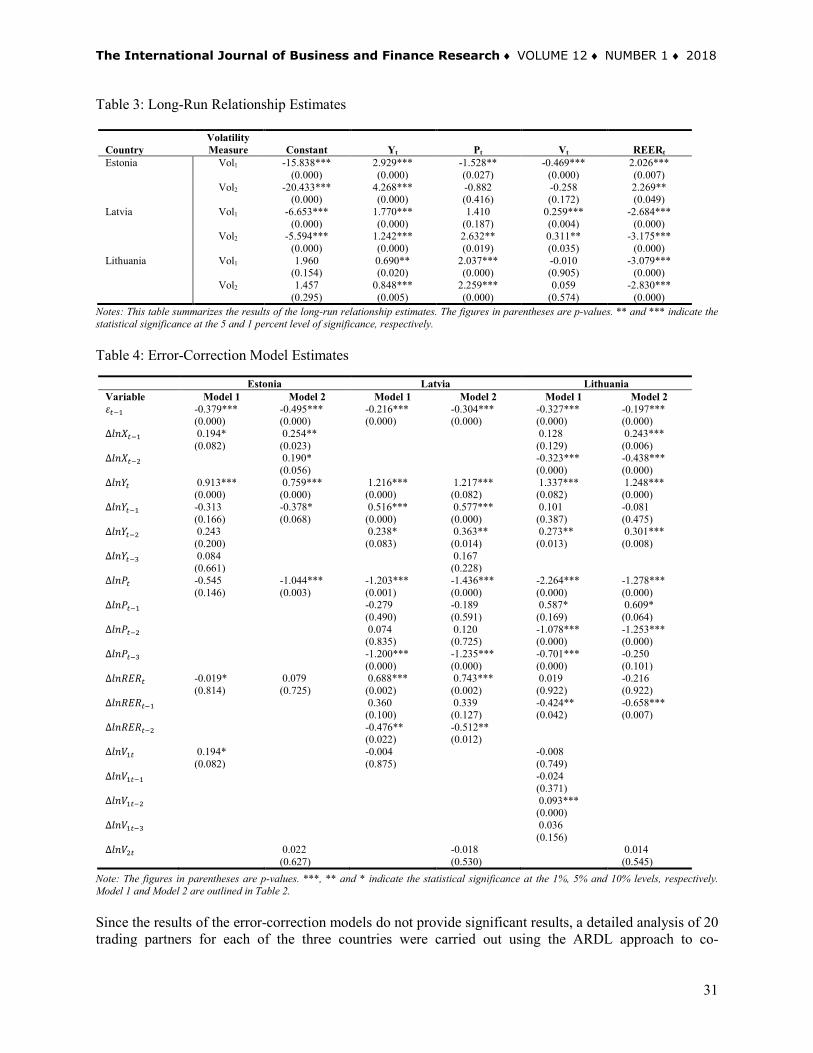
The International Journal of Business and Finance Research ♦ VOLUME 12 ♦ NUMBER 1 ♦ 2018
31
Table 3: Long-Run Relationship Estimates
Country
Volatility Measure
Constant
Yt
Pt
Vt
REERt
Estonia Vol1 -15.838*** (0.000)
2.929*** (0.000)
-1.528** (0.027)
-0.469*** (0.000)
2.026*** (0.007)
Vol2 -20.433*** (0.000)
4.268*** (0.000)
-0.882 (0.416)
-0.258 (0.172)
2.269** (0.049)
Latvia Vol1 -6.653*** (0.000)
1.770*** (0.000)
1.410 (0.187)
0.259*** (0.004)
-2.684*** (0.000)
Vol2 -5.594*** (0.000)
1.242*** (0.000)
2.632** (0.019)
0.311** (0.035)
-3.175*** (0.000)
Lithuania Vol1 1.960 (0.154)
0.690** (0.020)
2.037*** (0.000)
-0.010 (0.905)
-3.079*** (0.000)
Vol2 1.457 (0.295)
0.848*** (0.005)
2.259*** (0.000)
0.059 (0.574)
-2.830*** (0.000)
Notes: This table summarizes the results of the long-run relationship estimates. The figures in parentheses are p-values. ** and *** indicate the statistical significance at the 5 and 1 percent level of significance, respectively. Table 4: Error-Correction Model Estimates
Estonia Latvia Lithuania Variable Model 1 Model 2 Model 1 Model 2 Model 1 Model 2 𝜀𝜀𝑡𝑡−1 -0.379***
(0.000) -0.495*** (0.000)
-0.216*** (0.000)
-0.304*** (0.000)
-0.327*** (0.000)
-0.197*** (0.000)
∆𝑙𝑙𝑇𝑇𝑋𝑋𝑡𝑡−1 0.194* (0.082)
0.254** (0.023)
0.128 (0.129)
0.243*** (0.006)
∆𝑙𝑙𝑇𝑇𝑋𝑋𝑡𝑡−2 0.190* (0.056)
-0.323*** (0.000)
-0.438*** (0.000)
∆𝑙𝑙𝑇𝑇𝑌𝑌𝑡𝑡 0.913*** (0.000)
0.759*** (0.000)
1.216*** (0.000)
1.217*** (0.082)
1.337*** (0.082)
1.248*** (0.000)
∆𝑙𝑙𝑇𝑇𝑌𝑌𝑡𝑡−1 -0.313 (0.166)
-0.378* (0.068)
0.516*** (0.000)
0.577*** (0.000)
0.101 (0.387)
-0.081 (0.475)
∆𝑙𝑙𝑇𝑇𝑌𝑌𝑡𝑡−2 0.243 (0.200)
0.238* (0.083)
0.363** (0.014)
0.273** (0.013)
0.301*** (0.008)
∆𝑙𝑙𝑇𝑇𝑌𝑌𝑡𝑡−3 0.084 (0.661)
0.167 (0.228)
∆𝑙𝑙𝑇𝑇𝑃𝑃𝑡𝑡 -0.545 (0.146)
-1.044*** (0.003)
-1.203*** (0.001)
-1.436*** (0.000)
-2.264*** (0.000)
-1.278*** (0.000)
∆𝑙𝑙𝑇𝑇𝑃𝑃𝑡𝑡−1 -0.279 (0.490)
-0.189 (0.591)
0.587* (0.169)
0.609* (0.064)
∆𝑙𝑙𝑇𝑇𝑃𝑃𝑡𝑡−2 0.074 (0.835)
0.120 (0.725)
-1.078*** (0.000)
-1.253*** (0.000)
∆𝑙𝑙𝑇𝑇𝑃𝑃𝑡𝑡−3 -1.200*** (0.000)
-1.235*** (0.000)
-0.701*** (0.000)
-0.250 (0.101)
∆𝑙𝑙𝑇𝑇𝑅𝑅𝑅𝑅𝑅𝑅𝑡𝑡 -0.019* (0.814)
0.079 (0.725)
0.688*** (0.002)
0.743*** (0.002)
0.019 (0.922)
-0.216 (0.922)
∆𝑙𝑙𝑇𝑇𝑅𝑅𝑅𝑅𝑅𝑅𝑡𝑡−1 0.360 (0.100)
0.339 (0.127)
-0.424** (0.042)
-0.658*** (0.007)
∆𝑙𝑙𝑇𝑇𝑅𝑅𝑅𝑅𝑅𝑅𝑡𝑡−2 -0.476** (0.022)
-0.512** (0.012)
∆𝑙𝑙𝑇𝑇𝑉𝑉1𝑡𝑡 0.194* (0.082)
-0.004 (0.875)
-0.008 (0.749)
∆𝑙𝑙𝑇𝑇𝑉𝑉1𝑡𝑡−1 -0.024 (0.371)
∆𝑙𝑙𝑇𝑇𝑉𝑉1𝑡𝑡−2 0.093*** (0.000)
∆𝑙𝑙𝑇𝑇𝑉𝑉1𝑡𝑡−3 0.036 (0.156)
∆𝑙𝑙𝑇𝑇𝑉𝑉2𝑡𝑡 0.022 (0.627)
-0.018 (0.530)
0.014 (0.545)
Note: The figures in parentheses are p-values. ***, ** and * indicate the statistical significance at the 1%, 5% and 10% levels, respectively. Model 1 and Model 2 are outlined in Table 2. Since the results of the error-correction models do not provide significant results, a detailed analysis of 20 trading partners for each of the three countries were carried out using the ARDL approach to co-

C. Moslares & E. M. Ekanayake | IJBFR ♦ Vol. 12 ♦ No. 1 ♦ 2018
32
integration. Due to the large number of countries involved, the results of the unit-root tests and bounds tests for co-integration analysis are not reported. Following the studies by Bahmani-Oskooee and Harvey (2011), Bahmani-Oskooee and Hegerty (2009), Bahmani-Oskooee and Wang (2008, 2009), Bahmani-Oskooee and Mitra (2008), Bahmani-Oskooee and Kovyryalova (2008), and Bahmani-Oskooee and Ardalani (2006), we report only the short-run volatility coefficients and all the long-run coefficients. The estimated results for individual trading partners for Estonia, Latvia, and Lithuania are presented in Tables 5, 6, and 7, respectively. Table 5: Short-Run and Long-Run Coefficient Estimates: Estonia
Short-Run Coefficient Estimates Long-Run Coefficient Estimates Country
tVln∆ 1ln −∆ tV 2ln −∆ tV 3ln −∆ tV Constant tYln tPln tVln tRERln
Belgium -0.510** (0.024)
4.552 4.617*** (0.000)
-74.161 (0.238)
-0.424 (0.173)
75.392 (0.232)
Canada -0.344 (0.563)
-8.903 1.836 (0.499)
-5.384** (0.046)
-0.803* (0.090)
-0.662 (0.810)
China, P.R. 0.420 (0.855)
0.218 (0.347)
0.583** (0.018)
-3.479 1.610** (0.024)
7.336 (0.207)
-0.515* (0.096)
-5.292** (0.014)
Denmark -0.482** (0.019)
0.389* (0.065)
3.596 2.019 (0.119)
11.558 (0.648)
-0.303 (0.351)
-15.308 (0.548)
Finland -0.082 (0.440)
0.277** (0.016)
0.173 (0.117)
5.824 0.879 (0.292)
5.490 (0.305)
-0.162 (0.282)
-7.061 (0.214)
France 0.056 (0.993)
35.022 5.955** (0.020)
14.641 (0.374)
-1.231** (0.024)
-17.683 (0.282)
Germany 0.008 (0.909)
-0.164** (0.021)
0.169** (0.019)
77.427 2.071* (0.062)
86.254 (0.296)
0.015 (0.941)
-87.604 (0.288)
Italy -0.602* (0.074)
-0.645* (0.085)
0.274 (0.428)
0.887*** (0.006)
-23.547 5.083* (0.056)
-2.844 (0.577)
-1.122** (0.016)
1.373 (0.803)
Latvia -0.146*** (0.000)
0.037 (0.393)
0.114*** (0.008)
0.074* (0.087)
-3.035 2.140*** (0.000)
-0.795 (0.517)
-0.857** (0.015)
-2.926 (0.118)
Lithuania -0.025 (0.441)
-8.084 3.074*** (0.000)
2.226 (0.145)
-0.053 (0.452)
-1.347* (0.075)
Mexico 0.783 (0.606)
-2.141 (0.152)
-1.934 (0.190)
-3.859** (0.017)
-73.149 4.102 (0.181)
-42.999 (0.145)
2.037 (0.492)
5.697 (0.178)
Netherlands 0.115 (0.464)
0.063 (0.686)
-0.375** (0.022)
-7.743 7.742*** (0.000)
10.854 (0.792)
0.136 (0.331)
-11.064 (0.787)
Norway 0.158** (0.036)
-0.152** (0.046)
36.909 7.622 (0.109)
-4.419 (0.347)
0.049 (0.928)
5.271 (0.403)
Poland -0.010 (0.867)
-8.116 2.931*** (0.000)
-1.994 (0.137)
0.091 (0.651)
-0.087 (0.914)
Russian Federation
0.123** (0.026)
-0.095* (0.074)
18.015 1.824 (0.304)
1.562** (0.015)
0.142 (0.343)
4.141*** (0.001)
Spain 0.306 (0.371)
75.473 2.241** (0.013)
-26.257** (0.010)
1.525*** (0.000)
19.843* (0.052)
Sweden -0.080* (0.069)
12.203 3.299 (0.147)
-5.166** (0.020)
-1.035* (0.078)
0.227 (0.905)
Turkey 0.269 (0.354)
-1.093 4.875*** (0.000)
-1.219*** (0.000)
-0.218 (0.563)
-8.914*** (0.000)
United Kingdom
-0.229** (0.030)
0.584*** (0.000)
0.519*** (0.000)
0.187*** (0.000)
9.779 2.672** (0.014)
-3.144*** (0.000)
-0.881*** (0.000)
0.447 (0.268)
United States
-0.265 (0.522)
-6.993 8.482*** (0.004)
4.678** (0.049)
2.436* (0.058)
-4.734*** (0.000)
Note: This table summarizes the results obtained using the error-correction model defined in Equation (3). The figures in parentheses are absolute value of t-statistic. ** and * indicate the statistical significance at the 1% and 5% levels, respectively. Estonia: Short-Run Effects of Exchange Rate Volatility on Exports The short-run estimated coefficients on exchange rate volatility presented on the left panel in Table 5 reveal a mixture of negative and positive signs. There is also a variation in the significance of the exchange rate volatility on exports among individual countries in the short-run. Some of the coefficients are negative and statistically significant. Of the 20 countries, 13 of the countries have at least one statistically significant coefficient. In the case of the

The International Journal of Business and Finance Research ♦ VOLUME 12 ♦ NUMBER 1 ♦ 2018
33
United Kingdom, all coefficients are statistically significant up to 3 lags. Only four countries, namely, China, France, Spain and Turkey, have positive coefficients for all lags but most of these coefficients are statistically insignificant in the short-run. Estonia: Long-Run Effects of Exchange Rate Volatility on Exports The long-run coefficient estimates for Estonia are shown in the right panel of Table 5. As economic theory postulates, the real income variable renders a positive sign in all cases. This coefficient is statistically significant in thirteen of the 20 countries. The relative price variable displays the expected negative sign in twelve of the 20 countries and is statistically significant at the 1% or 5% level in seven of the 20 countries. This result is similar to those of Bahmani-Oskooee and Harvey (2011), Bahmani-Oskooee and Mitra (2008), Bahmani-Oskooee and Kovyryalova (2008), and Bahmani-Oskooee and Ardalani (2006). The estimated coefficients on exchange rate volatility show a mixture of negative and positive signs but the majority of the coefficients are negative. This coefficient is negative and statistically significant for Canada, China, France, Italy, Latvia, Sweden, and the United Kingdom. Our findings are somewhat similar to those of Bahmani-Oskooee and Hegerty (2009) and Bahmani-Oskooee and Wang (2008, 2009). Finally, the estimated coefficients on the real exchange rate show a mixture of negative and positive signs but the majority of the coefficients are negative. In general, in the long-run, exchange rate volatility appears to have mixed effect on the Estonian exports. Latvia: Short-Run Effects of Exchange Rate Volatility on Exports The short-run estimated coefficients on exchange rate volatility presented on the left panel in Table 6 reveal a mixture of negative and positive signs. There is also a significance variation of the exchange rate volatility on exports among individual countries in the short-run. Some of the coefficients are positive but only a very small number of coefficients are statistically significant. The countries that have negative coefficients show that most of the coefficients are statistically insignificant in the short-run. Latvia: Long-Run Effects of Exchange Rate Volatility on Exports The long-run coefficient estimates are shown in the right panel of Table 6. As hypothesized, the real income variable renders a positive sign in all cases. This coefficient is statistically significant at the 1% level in nine of the countries and significant at the 5% level in two countries. The relative price variable displays the expected negative sign in seventeen countries and is statistically significant in thirteen of the 20 countries. The estimated coefficients on the real exchange rate show a mixture of negative and positive signs but the majority of the coefficients are negative. Finally, the estimated coefficients on volatility also show a mixture of negative and positive signs and only six of the twenty are statistically significant. In general, in the long-run, exchange rate volatility appears to have mixed effect on the Latvian exports. Lithuania: Short-Run Effects of Exchange Rate Volatility on Exports The short-run estimated coefficients on exchange rate volatility for Lithuania presented on the left panel in Table 7 reveal a mixture of negative and positive signs. As in the case of Estonia and Latvia, there is also a significance variation of the exchange rate volatility on exports among individual countries in the short-run. Only a very small number of the coefficients are statistically significant. The countries that have negative coefficients show that these coefficients are statistically insignificant in the short-run, except Germany, Italy, and Sweden. Lithuania: Long-Run Effects of Exchange Rate Volatility on Exports The long-run coefficient estimates for Lithuania are shown in the right panel of Table 7. As expected, the real income variable renders a positive sign in all cases and it is statistically significant in most of the countries. The relative price variable displays the expected negative sign in all countries except China, Italy and the United States. The estimated coefficients on the real exchange rate show a mixture of negative and positive signs but the majority of the coefficients are negative. Finally, as in the case of Estonia and Latvia, the estimated coefficients on volatility show a mixture of negative and positive signs and only six of the twenty are statistically significant. Finland, France, Italy, Spain, and the United Kingdom have both negative and

C. Moslares & E. M. Ekanayake | IJBFR ♦ Vol. 12 ♦ No. 1 ♦ 2018
34
statistically significant coefficients on exchange rate volatility. In general, as in the case of Estonia and Latvia, the exchange rate volatility appears to have mixed effect on the Lithuanian exports in the long-run. Table 6: Short-Run and Long-Run Coefficient Estimates: Latvia
Country Short-Run Coefficient Estimates Long-Run Coefficient Estimates
tVln∆ 1ln −∆ tV 2ln −∆ tV 3ln −∆ tV Constant tYln tPln tVln tRERln
Belarus -0.007 (0.468)
-10.033 2.792*** (0.000)
-0.336*** (0.001)
-0.034 (0.429)
-0.245 (0.543)
Belgium 0.089 (0.636)
-1.792 2.812*** (0.001)
-3.196*** (0.000)
0.043 (0.714)
1.494** (0.019)
China, P.R. 0.119 (0.753)
-33.638 4.492*** (0.005)
8.437 (0.277)
-0.335 (0.743)
-6.069 (0.102)
Czech Republic
-0.089 (0.317)
-19.414 4.473* (0.052)
-2.711 (0.386)
-0.383 (0.582)
-0.376 (0.866)
Denmark -0.057 (0.413)
-3.241 3.020*** (0.002)
-5.247*** (0.000)
-0.133 (0.403)
2.979 (0.103)
Estonia -0.027 (0.413)
-3.056 2.564*** (0.000)
-4.452** (0.012)
-0.114 (0.651)
1.608 (0.448)
Finland 0.175 (0.279)
-0.104 (0.543)
0.305** (0.048)
-1.025 0.580 (0.484)
-2.345** (0.033)
-0.568*** (0.000)
-1.660 (0.248)
France -0.182 (0.441)
-5.744 1.005 (0.117)
-1.729* (0.056)
-0.512*** (0.000)
-0.659 (0.375)
Germany -0.121** (0.014)
0.028 (0.543)
-0.062 (0.168)
-4.590 2.217*** (0.000)
-1.939*** (0.000)
0.026 (0.688)
0.744** (0.040)
Italy -0.244* (0.087)
-27.454 0.771 (0.542)
1.451 (0.522)
-0.945*** (0.000)
-3.507* (0.087)
Lithuania 0.051 (0.229)
-5.524 2.479 (0.108)
-3.681 (0.271)
-0.046 (0.873)
0.951 (0.790)
Netherlands 0.100 (0.429)
-0.767 0.888 (0.133)
-2.716*** (0.001)
-0.111 (0.264)
-0.592 (0.412)
Norway 0.042 (0.597)
-26.691 1.717 (0.942)
-2.565 (0.556)
-0.366 (0.903)
-7.834 (0.805)
Poland -0.010 (0.867)
-8.116 2.931*** (0.000)
-1.994 (0.137)
0.091 (0.651)
-0.087 (0.914)
Russian Federation
-0.068 (0.203)
-0.161*** (0.002)
-0.079** (0.020)
-25.972 6.012*** (0.000)
-4.959** (0.014)
0.623 (0.289)
-9.393 (0.122)
Spain -0.487 (0.269)
-5.102 3.909*** (0.000)
-8.962*** (0.000)
-0.575** (0.012)
2.387* (0.058)
Sweden -0.234** (0.013)
3.008 0.058 (0.968)
-3.083*** (0.002)
-0.553 (0.166)
0.919 (0.375)
Turkey 0.338 (0.225)
-0.605** (0.024)
0.208 (0.456)
0.622** (0.021)
-57.780 4.218*** (0.000)
-0.671** (0.024)
1.091*** (0.001)
-2.274 (0.356)
United Kingdom
0.032 (0.451)
41.428 8.223** (0.029)
-2.663* (0.071)
-0.278*** (0.009)
2.299* (0.094)
United States
0.148 (0.295)
0.194 (0.245)
-0.216 (0.129)
0.172 (0.231)
-19.306 5.076** (0.019)
0.289 (0.911)
0.027 (0.928)
-0.965 (0.629)
Note: This table summarizes the results obtained using the error-correction model defined in Equation (3). The figures in parentheses are absolute value of t-statistic. ** and * indicate the statistical significance at the 1% and 5% levels, respectively. SUMMARY AND CONCLUSIONS In this paper we have examined the dynamic relationship between exports and exchange rate volatility in Baltic countries, in the context of a multivariate error-correction model. Estimates of the long-run export

The International Journal of Business and Finance Research ♦ VOLUME 12 ♦ NUMBER 1 ♦ 2018
35
demand functions were obtained by employing the bounds testing approach to co-integration using quarterly data for the period 1993Q1 – 2014Q4. Table 7: Short-Run and Long-Run Coefficient Estimates: Lithuania
Short-Run Coefficient Estimates Long-Run Coefficient Estimates Country
tVln∆ 1ln −∆ tV 2ln −∆ tV 3ln −∆ tV Constant tYln tPln tVln tRERln
Belarus -0.033*** (0.000)
-17.159 3.994*** (0.000)
-0.676*** (0.000)
-0.106** (0.012)
-0.476 (0.262)
Belgium -0.260 (0.142)
-10.062 2.191*** (0.002)
1.081 (0.143)
-0.252*** (0.004)
-0.923 (0.147)
Czech Republic
-0.073 (0.528)
0.167 (0.168)
-0.155** (0.207)
0.286** (0.020)
-9.103 2.412 (0.365)
-0.081 (0.986)
-0.747 (0.263)
-1.295 (0.606)
Denmark 0.032 (0.451)
-4.241 1.167 (0.255)
-0.581 (0.588)
-0.246*** (0.000)
-1.474* (0.091)
Estonia 0.044 (0.451)
-12.015 2.904*** (0.002)
0.480 (0.909)
-0.078 (0.673)
-1.731 (0.483)
Finland -0.045 (0.396)
-28.869 6.910 (0.427)
2.579 (0.612)
-0.454 (0.224)
4.620 (0.541)
France 0.020 (0.709)
-4.794 1.142 (0.569)
0.637 (0.703)
-0.212** (0.010)
-3.533*** (0.004)
Germany -0.021 (0.595)
0.026 (0.498)
-0.071* (0.068)
-0.080** (0.047)
7.040 0.152 (0.992)
-3.774 (0.780)
0.280 (0.906)
-0.152 (0.877)
Italy -0.154 (0.426)
-0.175 3.868*** (0.000)
-5.156*** (0.000)
-0.710*** (0.000)
3.106*** (0.000)
Latvia 0.045 (0.432)
-6.482 1.984 (0.128)
4.511* (0.071)
0.058 (0.768)
1.677 (0.515)
Netherlands -0.097 (0.247)
-0.088 (0.280)
0.089 (0.268)
-0.357*** (0.000)
-6.862 3.181 (0.312)
4.456 (0.440)
-0.101 (0.667)
-8.228* (0.086)
Norway 0.028 (0.676)
42.818 9.202*** (0.001)
9.500*** (0.001)
0.283 (0.496)
-8.018*** (0.000)
Poland -0.045 (0.382)
-0.040 (0.519)
-0.101 (0.135)
-0.237*** (0.000)
-10.516 3.390*** (0.000)
-0.471 (0.375)
0.083 (0.648)
-0.228 (0.846)
Russian Federation
-0.029*** (0.001)
0.030*** (0.005)
0.036*** (0.000)
16.056 0.301 (0.848)
1.479*** (0.003)
-0.193 (0.114)
4.412*** (0.000)
Spain 0.138 (0.593)
0.537** (0.039)
-12.871 6.272*** (0.006)
-6.269** (0.045)
-0.966*** (0.000)
5.174** (0.033)
Sweden 0.481 (0.725)
0.702 (0.601)
-0.562 (0.652)
-1.627* (0.070)
-6.630 1.995 (0.691)
2.016 (0.655)
0.008 (0.986)
-2.515 (0.414)
Turkey -0.102 (0.313)
-0.097 (0.396)
0.008 (0.939)
-0.287*** (0.008)
-0.664 1.136 (0.390)
1.073** (0.024)
0.185 (0.705)
2.125 (0.480)
Ukraine -0.061 (0.467)
-1.134 2.567 (0.173)
3.117*** (0.001)
-0.023 (0.939)
5.151*** (0.002)
United Kingdom
0.001 (0.997)
-0.139*** (0.002)
0.008 (0.859)
-0.149*** (0.001)
-7.818 4.606 (0.814)
-5.476 (0.845)
2.225 (0.844)
-1.535 (0.913)
United States -0.062 (0.645)
0.072 (0.589)
-0.285** (0.029)
-11.516 4.017* (0.054)
3.974** (0.019)
-0.122 (0.499)
-3.483*** (0.002)
Note: This table summarizes the results obtained using the error-correction model defined in Equation (3). The figures in parentheses are absolute value of t-statistic. ** and * indicate the statistical significance at the 1% and 5% levels, respectively. The co-integration results clearly show that there exists a long-run equilibrium relationship between real exports, real foreign income, relative prices, real exchange rate, and real exchange rate volatility, in all three countries selected. In the long-run, all the specifications yielded expected signs for the coefficients. Most of our estimated coefficients are statistically significant either at the 1% or 5% levels. There is also a significance variation of the exchange rate volatility on exports among countries in the short-run. Some of the coefficients are negative and statistically significant while others are positive and statistically insignificant in the short-run. There is also a significant variation of the exchange rate volatility on exports among countries in the short-run. Some of the coefficients are negative and statistically significant. These results point out to the increasing competitiveness of Baltic countries’ exports in the global economy as a result of the depreciating value of the local currency over time. It underscores the degree to which transition countries such as Estonia, Latvia and Lithuania have succeeded in finding alternative markets in Europe and especially in Asia in the last decade. One of the limitations of the

C. Moslares & E. M. Ekanayake | IJBFR ♦ Vol. 12 ♦ No. 1 ♦ 2018
36
present study is the limited number of countries included in the study. While the current study considered only top 20 export destinations for each of the three Baltic countries, more meaningful conclusions would have been attained if the number of countries is increased. Future research on the topic will cover all export destinations. Future research will also carry out the analysis by including all countries in the Central Europe and Baltic countries. REFERENCES Aristotelous, K. (2001). ‘Exchange rate volatility, exchange rate regime, and trade volume: evidence from UK-US export function (1889-1999)’, Economic Letters, 72(1), pp. 87-94. Arize, A. C. (1998). ‘The effects of exchange-rate volatility on U.S. imports: an empirical investigation’, International Economic Journal, 12(2), pp. 31-40. Arize, A. C. (1996). ‘The impact of exchange-rate uncertainty on U.S. export growth: evidence from Korean data’, International Economic Journal, 10(3), pp. 49-60. Arize, A. C. (1995). ‘The effects of exchange-rate volatility on U.S. exports: an empirical investigation’, Southern Economic Journal, 62(1), pp. 34-43. Arize, A. C., Osang, T., Slottje, D. J. (2000). ‘The exchange rate volatility and foreign trade: evidence from thirteen LDCs’, Journal of Business and Economic Studies, 18, pp. 10-17. Assery, A., Peel. D. A. (1991). ‘The effects of exchange rate volatility on exports: some new estimates’, Economic Letters, 37(3), pp. 173-177. Bahmani-Oskooee, M., Harvey, H. (2011). ‘Exchange-rate volatility and industry trade between the U.S. and Malaysia’, Research in International Business and Finance, 25(2), pp. 127-155. Bahmani-Oskooee, M., Hegerty, S. W. (2009). ‘The effects of exchange-rate volatility on commodity trade between the United States and Mexico’, Southern Economic Journal, 75(4), pp. 1019–1044. Bahmani-Oskooee, M., Hegerty, S. W. (2007). ‘Exchange rate volatility and trade flows: a review article’, Journal of Economic Studies, 34(2), pp. 211-255. Bahmani-Oskooee, M., Kovyryalova, M. (2008). ‘Impact of exchange rate uncertainty on trade flows: evidence from commodity trade between the United States and the United Kingdom’, The World Economy, 31(8), pp. 1097-1128. Bahmani-Oskooee, M., Mitra, R. (2008). ‘Exchange rate risk and commodity trade between the U.S. and India’, Open Economies Review, 19(1), pp. 71–80. Bahmani-Oskooee, M., Wang, Y. (2009). ‘Exchange rate sensitivity of Australia’s trade flows: evidence from industry data’, The Manchester School, 77(1), pp. 1-16. Bahmani-Oskooee, M., Wang, Y. (2008). ‘Impact of exchange rate uncertainty on commodity trade between the U.S. and Australia’, Australian Economies Papers, 47(3), pp. 235-258. Bahmani-Oskooee, M., Ardalani, Z. (2006). ‘Exchange rate sensitivity of U.S. trade flows: evidence from industry data’, Southern Economic Journal, 72, pp. 542–559.

The International Journal of Business and Finance Research ♦ VOLUME 12 ♦ NUMBER 1 ♦ 2018
37
Bahmani-Oskooee, M. (2002). ‘Does black market exchange rate volatility deter the trade flows? Iranian experience’, Applied Economics, 34, pp. 2249-2255. Bahmani-Oskooee, M. (1991). ‘Exchange rate uncertainty and trade flows of developing countries’, The Journal of Developing Areas, 25, pp. 497-508. Bahmani-Oskooee, M., Payesteh, S. (1993). ‘Does exchange rate volatility deter trade volume in LDCs’, Journal of Economic Development, 18(2), pp. 189-205. Bredin, D., Fountas, S., Murphy, E. (2003). ‘An empirical analysis of short-run and long-run Irish export functions: does exchange rate volatility matter?’, International Review of Applied Economics, 17(2), pp. 193-208. Byrne, J., Darby, J., MacDonald, R. (2008). ‘US trade and exchange rate volatility: a real sectoral bilateral analysis’, Journal of Macroeconomics, 30, pp. 238-259. Choudhry, T. (2005). ‘Exchange rate volatility and the United States exports: evidence from Canada and Japan’, Journal of Japanese and International Economies, 19, pp. 51-71. Chowdhury, A. R. (1993). ‘Conditional exchange rate volatility depresses trade flows? Evidence from error-correction models’, Review of Economic and Statistics, 75, pp. 700-706. Chowdhury, A. R., Wheeler, M. (2008). ‘Does exchange rate volatility affect foreign direct investment? Evidence from four economies’, The International Trade Journal, 22(2), pp. 218-245. Chou, W. L. (2000). ‘Exchange rate variability and China’s exports’, Journal of Comparative Economics, 28(1), pp. 61-79. De Vita, G., Abbott, A. (2004). ‘Real exchange rate volatility and US exports: An ARDL bounds testing approach’, Economic Issues, 9(1), pp. 69-78. Doyle, E. (2001). ‘Exchange rate volatility and Irish-UK trade, 1979-1992’, Applied Economics, 33, pp. 249-265. Gheong, C., Mehari, T., Williams, L. V. (2005). ‘The effects of exchange rate variability on price competitiveness and trade volumes in the U.K.: A disaggregated approach’, Journal of Policy Modeling, 27(8), pp. 961-970. Hooper, P., Kohlhagen, S. (1978). ‘Real exchange rate uncertainty on the prices and volume of international trade’, Journal of International Economics, 8, pp. 483-511. International Monetary Fund (2016), International Financial Statistics Database. International Monetary Fund (2016), Direction of Trade Database. Koray, F., Lastrapes, W. D. (1989). ‘Real exchange rate volatility and the U.S. bilateral trade: A VAR approach’, Review of Economics and Statistics, 71(11), pp. 708-712. Kroner, K. F., Lastrapes, W. D. (1993). ‘The impact of exchange rate volatility on international trade: reduce form estimates using the GARCH-in-Mean model’, Journal of International Money and Finance, 12(6), pp. 218-318.

C. Moslares & E. M. Ekanayake | IJBFR ♦ Vol. 12 ♦ No. 1 ♦ 2018
38
McKenzie, M. D., Brooks, R. D. (1997). ‘The impact of exchange rate volatility on German-US trade flows’, Journal of International Financial Markets, Institutions and Money, 7(1), pp. 73-87. Onafowora, O. A., Owoye, O. (2008). ‘Exchange rate volatility and export growth in Nigeria’, Applied Economics, 40(12), pp. 1547-1556. Ozturk, I., Kalyonku, H. (2009). ‘Exchange rate volatility and trade: an empirical investigation from cross-country comparisons’, African Development Review, 21(3), pp. 499-513. Pesaran, M., Shin, Y., Smith, R. (2001). ‘Bounds testing approaches to the analysis of level relationships’, Journal of Applied Econometrics, 16(3), pp 289-326. Pino, G., Tas, D., Sharma, S. C. (2016). ‘An investigation of the effects of exchange rate volatility on exports in East Asia, Applied Economics, 48(26), pp 2397-2411. Qian, Y., Varangis, P. (1994). ‘Does exchange-rate volatility hinder export growth?: additional evidence’, Empirical Economics, 98, pp. 138-148. Weliwita, A., Ekanayake, E. M., Tsujii, H. (1999). Real exchange rate volatility and Sri Lanka's exports to the developed countries, 1978-96’, Journal of Economic Development, 24(1), pp. 147-165. BIOGRAPHY Dr. Carlos Moslares is the Dean of the IQS School of Management, Universitat Ramon Llull, Spain. He earned his Ph.D. at the Florida International University. Contact information: Universidad Ramon Llull, IQS School of Management, Via Augusta, 390, 08017, Barcelona, Spain. Phone: +34 932 672 000 or +34 932 056 266. E-mail: [email protected]. Dr. E. M. Ekanayake is a Professor of Economics at Bethune-Cookman University, Daytona Beach, Florida, USA. He earned his Ph.D. in Economics at the Florida International University, Miami in 1996. He has many publications to his credit. Contact information: College of Business and Entrepreneurship, Bethune-Cookman University, 640 Dr. Mary McLeod Bethune Blvd., Daytona Beach, FL 32114, USA. Phone: (386) 481-2819. E-mail: [email protected].

The International Journal of Business and Finance Research Vol. 12, No. 1, 2018, pp. 39-56 ISSN: 1931-0269 (print) ISSN: 2157-0698 (online)
www.theIBFR.com
39
LABEL CO-MOVEMENT: COMPONENT STOCK
INCLUSION AND EXCLUSION BETWEEN DIFFERENT EXCHANGE-TRADED FUNDS
Chun-An Li, National Yunlin University of Science and Technology Min-Ching Lee, National Yunlin University of Science and Technology
Ju-Hua Liu, National Yunlin University of Science and Technology
ABSTRACT This study examines the co-movement phenomenon in Taiwan’s stock markets. We investigate this phenomenon both before and after the inclusion and exclusion of component stocks from the Taiwan 50 or Taiwan 100 indices in terms of changes in component stock returns and turnover co-movement relationships. In addition to providing a sample analysis, this study explores consistency in changes to co-movement relationships owing to market status (bull or bear) or investor sentiment (overly optimistic, optimistic, pessimistic, and overly pessimistic). The empirical results reflect the stocks’ returns or turnover. For example, apart from periods of overly pessimistic sentiment, including and excluding components in the Taiwan 100 or Taiwan 50 indices generally reveals a strengthened co-movement relationship with the new group and a weakened link with the original group, regardless of a bull or bear market. The result is consistent with Boyer’s (2011) label argument on co-movement. However, a subtler perspective reveals a rather insignificant change in the co-movement relationship for stock returns as components move from the Taiwan 50 to the Taiwan 100 index. JEL: G12 KEYWORDS: Co-Movement, Label Effect, Exchange-Traded Funds INTRODUCTION
abel Co-movement” represents assets having the same label, which results in them moving in the same direction in terms of returns or turnover. In other words, when assets have the same style and are classified to be the same label, we can expect their returns to change in line with
similar trends. Therefore, according to Boyer’s (2011) argument, labels induce excess covariation in returns through the trading activity of investors, who allocate capital across styles delineated by these labels. Many theoretical and empirical studies examine the co-movement phenomenon in financial markets. According to conventional finance theory, the fundamentals of securities or the market’s macroeconomics primarily cause this co-movement. However, according to the efficient market hypothesis, the price of a financial asset reflects all publicly available or hidden “insider” information relevant to its value without human behavioral influence, such as optimistic or pessimistic sentiment. Further, the excess returns of the capital asset pricing model (CAPM) reflects stocks’ systematic risk, which also indicates both strong or weak correlations between securities and the market. However, several studies on behavioral finance find that the fundamentals do not completely explain the co-movement phenomenon (For example, the Siamese Twins co-movement noted by Froot and Dabora (1999); research by Barberis, Shleifer, and Wurgler (2005) and Boyer (2011); Claessens and Yafeh’s (2012) finding of index co-movement; Pirinsky and Wang’s (2006) study on regional HQ comovement; Muslu, Rebello, and Xu’s (2014) study on recommendation co-movement by sell-side analysis; Kumar and Lee’s (2006) co-movement study of individual shareholders’
“L

CA. Li et al | IJBFR ♦ Vol. 12 ♦ No. 1 ♦ 2018
40
sentiment; and Kumar, Page, and Spalt’s (2016) research on co-movement and gambling motives). Jin and Myers (2006) argue that co-movement that is not driven by fundamentals could indicate a company’s lack of specific information. Barberis, Shleifer and Wurgler (2005) argue that volatility in investor sentiment based on specific habitats or categories could lead to non-fundamental co-movement. Kumar, Page, and Spalt (2016) study trading with the intent to gamble, with a focus on lottery-type stocks, and reveal returns co-movement within this stock category. Alternatively, Brockman, Liebenberg, and Schutte (2010) and Veldkamp (2006) find that information plays an important role in co-movement. Muslu, Rebello, and Xu (2014) reveal evidence implying that stock co-movement occurred during analysts’ forecast of earnings announcements. Höchstötter, Meyer, Riordan, and Storkenmaier (2014) also discover that news could lead to stock co-movement. However, Kumar and Lee (2006) demonstrate that high-ratio individuals’ trading and sentiments could explain returns co-movements. However, neither macroeconomic news nor analysts’ earnings forecast revisions can explain such a phenomenon. Barberis and Shleifer (2003) propose their labeling argument to explain non-fundamental co-movement, stating that for the sake of simplicity, investors first categorize stocks in terms of their styles and then label them. Investors then allocate their assets among different labels, after which the co-movement phenomenon can occur (Labeling can simplify investment, as the investor will only need to reallocate assets among some specified labels, which differs from style investing). Boyer (2011) finds that an economically insignificant stock index could lead to co-movement in returns beyond its fundamentals. When a value stock is included in a growth index, the stock return co-moves with the new growth index; however, it has less of a co-movement relationship with the original category. The opposite occurs when a growth stock becomes a value stock, in which the co-movement of the value index and return increases, and the correlation with growth stocks decreases. Boyer (2011) confirms that this result could explain the labeling theory. Claessens and Yafeh (2012) examine data from 40 developed and developing countries’ stock that is newly included in the primary index, and find co-movement between the stock price and primary index, especially in those stocks with a low systematic risk (β). Behavioral finance studies generally conclude that systematic psychological bias could significantly affect pricing (Kahneman and Tversky, 1979, Armstrong and Fildes, 1984, Becker and Kuhn, 1984). The label phenomenon is a psychological bias involving a representativeness heuristic, implying that the use of experience serves as a reference for thinking, evaluating, and decision-making, to save time and improve efficiency. Boussaidi (2013), Luo (2013), and Liu and Du (2016) study the representativeness heuristic; the label effect is also a representativeness heuristic in that investors will make decisions using specific experiences in uncertain situations. For example, a company’s past success could serve as its “representativeness” to lead investors’ experience of good performance in the future. Reinforced by the representativeness heuristic concept, investors tend to overreact to a company’s continuous outstanding profit. An exchange-traded fund (ETF) is a fund that passively tracks the performance of a benchmark index with a specific style. An ETF’s component stock is not actively decided by the fund manager, but passively determined by tracking the underlying index. Once the underlying index includes or excludes a proportion of the constituent stocks, the ETF should also follow by adjusting the proportion of its portfolio. Essentially, investors allocate their assets in ETF by tracking the performance of the index’s style. We label those ETFs according to various styles. Therefore, by the various labels of ETF’s returns and turnover, we can trace how the indices of those ETFs perform. Our study of label co-movement involves tracing how the indices of various labeled ETFs perform. We use the reorganization of component stocks to investigate changes in their ETF indices before and after the co-movement relationships with the original and new groups. The Taiwan 50 (TWN50) and Taiwan 100 (TM100) indices are types of ETFs that are excluded from the TWN50 and included in the TM100, or vice versa. The TWN50 includes a combination of stocks of 50

The International Journal of Business and Finance Research ♦ VOLUME 12 ♦ NUMBER 1 ♦ 2018
41
listed companies with the greatest market capitalization and highest stability. The TM100 further includes the 51st to the 150th component stocks. Investors may consequently label companies differently for the TWN50 and TM100, resulting in a label switch in returns or turnover co-movement relationships with the same group’s ETF index. Prior studies generally investigate the co-movement phenomenon of individual stocks included or excluded in the primary index. They rarely focus on the co-movement phenomenon switch with ETF. However, we investigate the reorganized component ETF stock, and thus provide new evidence regarding label co-movement. Stock liquidity and stability increases when the component stock is included in the TWN50 and excluded from the TM100, and alternatively, decreases when the component stock is excluded from the TWN50 and included in the TM100. Component reorganization also implies a label switch, from a good label to a poor label, and vice versa. Our study’s economic implications of label co-movement differ slightly from those of Boyer’s (2011); unlike us, the author has not addressed co-movement relationships with turnover. This study also emphasizes market sentiment to determine any variations in changes to co-movement relationships in stock returns and turnover under different market sentiments (overly optimistic, optimistic, pessimistic, and overly pessimistic) and status (bull or bear market). Our results indicate that component stocks switch from the TM100 to TWN50 indices and vice versa. However, except during the overly pessimistic period, including whole samples, market status (bull or bear market), and pessimistic market sentiment, will have increased co-movement relationships in stock returns and turnovers with the new group, and decreased links with the original group. This is broadly consistent with Boyer’s (2011) labeling theory. However, the switch in a component stock from the TWN50 to the TM100 index indicates an insignificant co-movement relationship. It also indicates that investors would recognize significant differences when component stocks switch to a better label category, weakening the co-movement relationship with the original group and strengthening the new tie. Conversely, the opposite switch would have no profound impact on recognition because the co-movement relationship exhibits no apparent change. This paper has five sections. The first section consists of the introduction. The second section includes a literature review discussing various references to the label effect and co-movement phenomenon. The third section describes the research method, hypothesis, research design model, sample, and operationally defines the research variables. The fourth section provides an empirical analysis, and the final section concludes and offers recommendations. LITERATURE REVIEW Barberis and Shleifer’s (2003) theoretical model first proposed the label effect. When an investor prefers a specifically labeled stock, stock co-movement in the same style increases, and the relationship with the new category strengthens. They infer that the label switch leads to a higher co-movement relationship with the new label group. This study explores the label effect of a strengthening or weakening co-movement relationship in the returns and turnover during the switching of an ETF component stock, as stock return co-movement indicates significant covariance between the individual component stock and its corresponding index. Early literature, such as that of Vijh (1994), discovers a significant increase in the β in evaluating the covariant relationships of individual and market returns for a component stock included in the S&P 500 index. Wurgler and Zhuravskaya (2002) note similar results regarding the increase in co-movement for component stocks included in the S&P 500 index. Many studies explore the co-movement relationships between component stock and index in returns when the component stock is included in the index, including those of Harris and Gurel (1986), Shleifer (1986), Lynch and Mendenhall (1997), Kaul, Mehrotra, and Morck (2000), Greenwood and Sosner (2007), and

CA. Li et al | IJBFR ♦ Vol. 12 ♦ No. 1 ♦ 2018
42
Greenwood (2005). They find that the β and R2 (coefficients of determination) of both the component stock and index increase with inclusion and decrease with exclusion. Barberis, Shleifer, and Wurgler (2005) use Vijh’s (1994) research exploring the co-movement phenomenon for component stock returns on the S&P 500 index from both the conventional and psychological perspectives. The former refers to co-movement resulting from the spread of fundamentals, while the latter emphasizes co-movement owing to investor sentiment. In addition, they divide the psychological perspective into three views: category, habitat, and information diffusion. Barberis and Shleifer (2003) propose the category view, which refers to the simplified investment strategy wherein investors prefer to allocate their assets according to specifically labeled stock categories such as small-cap, value stocks, and so on. The labeling factor in investors’ decision-making processes could affect a category’s stock price. Essentially, when investors move their investment from one category to another, category stocks with the same label convey the returns’ co-movement, regardless of the stock’s fundamentals. Barberis, Shleifer, and Wurgler (2005) argue that as a component stock is included in the S&P 500 index, its β increases and develops a co-movement relationship with the S&P 500 index, which its fundamentals cannot explain. Boyer (2011) studies component stocks on the S&P/Barra index and uses the book-to-market (BM) ratio to differentiate them as value and growth stocks, and reclassifies stock labels according to changes in their BM ratios. Boyer’s research reveals a significant co-movement relationship among stocks of the same style. Further, this switch from the original to new style results in a strong co-movement in stock returns and turnover with the new style group, as well as a weaker link with the original. The S&P/Barra index could serve as an important indicator for category stock, either “value” or “growth,” among which investors allocate their assets. Therefore, Boyer (2011) argues that style investment generally implies investors’ psychological bias, causing significant co-movement in category stocks with the same BM value. We explore the label co-movement of reorganized component stocks in the ETF. This differs from Boyer’s (2011) work, which focuses on style label changes for value and growth stocks. We also investigate the perceptions of component stocks with different labeling. The TWN50 represents the best 50 component stocks with liquidity and stability, followed by the TM100. The inclusion of component stock in the TWN50 from the TM100 implies an upgrade in its image, and vice versa for a downgrade. Additionally, prior studies do not discuss turnover co-movement or label changes in accordance with market status, which our research includes. Our study categorizes the sentiment for market status as overly optimistic, optimistic, pessimistic, and overly pessimistic, to observe the differences not only in this relationship, but also in the bull or bear market classification. DATA AND METHODOLOGY Data Based on Barberis and Shleifer’s (2003) labeling theory, as well as Barberis, Shleifer, and Wurgler’s (2005) and Boyer’s (2011) empirical analyses of index component stock co-movement, we hypothesize that the co-movement phenomenon will also occur during the reorganization of component stocks in the TWN50 and TM100 indices. Therefore, we utilize data for component stocks in the TWN50 and TM100 indices as the research sample. The sample period is from January 1, 2006, to May 31, 2015, and contains about 2,332 daily observations. The TWN50 is an ETF with components that include a combination of stocks from the 50 listed companies with the greatest market capitalization and the highest stability in Taiwan’s stock market. Similarly, the TM100 includes the 51st to the 150th component stocks. We use component stocks that move between the TM100 and TWN50, and vice versa, as our sample. We assume that before the switch from the original group, the co-movement relationship would significantly decrease between the stock returns or turnover

The International Journal of Business and Finance Research ♦ VOLUME 12 ♦ NUMBER 1 ♦ 2018
43
and the original ETF index (hereafter the “original” and “new” groups, respectively). Moreover, after the switch to the new group, the co-movement relationship would significantly increase between stock returns or turnover and the new ETF index. This data is sourced from the Taiwan Economic Journal (TEJ). We base our analysis on Barberis and Shleifer (2003) and Boyer’s (2011) theory of label co-movement. The TWN50 ETF in Taiwan provides investors with a benchmark for large-cap companies. This index measures the performance of large-cap companies, reflecting the distinctive top-50 firms by market capitalization. The components of the TWN50 generally have greater market capitalization, higher liquidity, and stable returns characteristics in this market segment. The TM100 is a mid-cap index of ETFs, with medium-sized market capitalization, relatively unstable returns, and lower liquidity. A label switch indicates that a component stock is included in the ETF and excluded from another ETF. The study excludes 27 component stocks from the TM100 and includes them in the TWN50, while 28 component stocks switched in the opposite direction. Variable Definition We calculate the returns and turnover of the component stocks on the TWN50 and TM100 weighted on market capitalization to test for any change in the weighted returns and turnover co-movement relationship of the component stock in the original or new group, before and after the adjustment. To observe the changes in co-movement relationships, we further divide the research market status into bull and bear periods, and market sentiments into optimistic, overly optimistic, pessimistic, and overly pessimistic in accordance with the TAIEX options volatility index. According to Fabozzi and Francis’ (1979) market status classification, the TAIEX options volatility index increasing over a three-month period serves as an indication of a bull market; conversely, a decrease over a three-month period indicates a bear market. According to the TAIEX options volatility index, market sentiment is classified with the values of under 15, 15–20, 21–40, and over 40 as thresholds for the 4 sentiments: overly optimistic, optimistic, pessimistic, and overly pessimistic (Chen and Zhou, 2014). Established in 1997, the TAIEX options volatility index applies the volatility index (VIX) methodology from the Chicago Board Options Exchange (CBOE) to trading activity in Taiwan’s options market. This accurately reflects the market’s current price volatility, which provides options traders with more information to help them evaluate market conditions and make appropriate trading decisions. The VIX utilizes S&P 100 index options prices to generate and imply volatility. This reflects the market’s expectations of future market volatility to provide options traders with more information to plan their trading and hedging strategies, and offer a more practical and balanced perspective on the market’s outlook. Generally, while a higher VIX indicates that traders expect greater volatility in the equities market, a lower VIX indicates that they expect lower volatility in the equities market. Serving as a reflection of the change in investor sentiment, the index has long been known as the “investor fear gauge.” Test of ETF Component Stock Returns’ Co-Movement This study adopts Boyer’s (2011) method to test the average coefficients’ change in Equation (1). We regress the component stock on the ETF index for the returns’ co-movements phenomenon before or after the event date of inclusion and exclusion from the TWN50 and TM100. 𝑟𝑟𝑖𝑖𝑖𝑖 = 𝛽𝛽𝑖𝑖𝑖𝑖 + 𝛽𝛽𝑖𝑖𝑖𝑖𝑟𝑟𝑖𝑖𝑖𝑖 + 𝛽𝛽𝑖𝑖𝑖𝑖𝑟𝑟𝑖𝑖𝑖𝑖 + 𝑒𝑒𝑖𝑖𝑖𝑖 (1) In Equation (1), 𝑟𝑟𝑖𝑖𝑖𝑖 : Daily log returns of the reorganized component stock

CA. Li et al | IJBFR ♦ Vol. 12 ♦ No. 1 ♦ 2018
44
𝑟𝑟𝑖𝑖𝑤𝑤 : Weighted daily log returns of the TWN50 index
𝑟𝑟𝑖𝑖𝑖𝑖 : Weighted daily log returns of the TM100 index The event date is the day of exclusion and inclusion of the component stocks, either as the switch from the TM100 to the TWN50 or vice versa. We use Equation (1) to regress the individual component stocks on the ETF index for the returns’ co-movement phenomenon before and after one-month to six-months to the event day. Further, we test for the statistical significance of β’s average change before and after one month to six months to the event date using equations (2a) and (2b) as follows:
∆�̅�𝛽𝑖𝑖 = �𝛽𝛽𝑖𝑖𝑖𝑖𝑝𝑝𝑝𝑝𝑖𝑖 − 𝛽𝛽𝑖𝑖𝑖𝑖
𝑝𝑝𝑤𝑤𝑝𝑝
𝑛𝑛
𝑛𝑛
𝑖𝑖=1
(2a)
∆�̅�𝛽𝑖𝑖 = �𝛽𝛽𝑖𝑖𝑖𝑖𝑝𝑝𝑝𝑝𝑖𝑖 − 𝛽𝛽𝑖𝑖𝑖𝑖
𝑝𝑝𝑤𝑤𝑝𝑝
𝑛𝑛
𝑛𝑛
𝑖𝑖=1
(2b)
In Equations (2a) and (2b), 𝛽𝛽𝑝𝑝𝑤𝑤𝑝𝑝 , 𝛽𝛽𝑝𝑝𝑝𝑝𝑖𝑖: The estimate of regression before and after the event date, respectively. n: The number of reorganized component stocks. w, m: The regressions of component stocks on the TWN50 and TM100, respectively. According to Boyer’s (2011) label co-movement theory, for the component stocks switching from TM100 to TWN50, we expect the degree of co-movement of the TWN50’s returns to increase with a positive ∆β�𝑖𝑖. Conversely, we expect the degree of co-movement of the TM100’s returns to decrease with a negative ∆β�𝑖𝑖. The null and alternative hypotheses for this test are as follows:
�𝐻𝐻0: ∆ �̅�𝛽𝑖𝑖 ≤ 0 𝐻𝐻1: ∆ �̅�𝛽𝑖𝑖 > 0
�𝐻𝐻0: ∆ �̅�𝛽𝑖𝑖 ≥ 0 𝐻𝐻1: ∆ �̅�𝛽𝑖𝑖 < 0
(3a)
In contrast, when a component stock switches from the TWN50 to the TM100, we expect a negative ∆β�𝑖𝑖 and a positive ∆β�𝑖𝑖, respectively; the null and alternative hypothesis are as follows:
�𝐻𝐻0: ∆ �̅�𝛽𝑖𝑖 ≥ 0 𝐻𝐻1: ∆ �̅�𝛽𝑖𝑖 < 0
�𝐻𝐻0: ∆ �̅�𝛽𝑖𝑖 ≤ 0 𝐻𝐻1: ∆ �̅�𝛽𝑖𝑖 > 0
(3b)
Test of ETF Component Stock Turnovers’ Co-Movement This study uses the average coefficients’ change in Equation (4) to indicate the regression of the component stock on the ETF index for the turnovers’ co-movement phenomenon before and after the event date of inclusion and exclusion from the TWN50 and the TM100. 𝜏𝜏𝑖𝑖𝑖𝑖 = 𝜃𝜃𝑖𝑖𝑖𝑖 + 𝜃𝜃𝑖𝑖𝑖𝑖𝜏𝜏𝑖𝑖𝑖𝑖 + 𝜃𝜃𝑖𝑖𝑖𝑖𝜏𝜏𝑖𝑖𝑖𝑖 + 𝑒𝑒𝑖𝑖𝑖𝑖 (4) In Equation (4), τ𝑖𝑖𝑖𝑖 : Daily turnover of the reorganized component stock 𝜏𝜏𝑖𝑖𝑖𝑖 : Daily turnover of the TWN50 index

The International Journal of Business and Finance Research ♦ VOLUME 12 ♦ NUMBER 1 ♦ 2018
45
𝜏𝜏𝑖𝑖𝑖𝑖 : Daily turnover of the TM100 index We exclude component stocks from the TM100 and include them in the TWN50, or exclude them from the TWN50 and include them in the TM100. We then regress the individual component stocks on the ETF index for the turnovers’ co-movement phenomenon before and after one-month to six-months to the event day in Equation (4). Further, we test for the statistical significance of β’s average change before and after one-month to six-months to the event date, using equations (5a) and (5b).
∆�̅�𝜃𝑖𝑖 = �𝜃𝜃𝑖𝑖𝑖𝑖𝑝𝑝𝑝𝑝𝑖𝑖 − 𝜃𝜃𝑖𝑖𝑖𝑖
𝑝𝑝𝑤𝑤𝑝𝑝
𝑛𝑛
𝑛𝑛
𝑖𝑖=1
(5a)
∆�̅�𝜃𝑖𝑖 = �𝜃𝜃𝑖𝑖𝑖𝑖𝑝𝑝𝑝𝑝𝑖𝑖 − 𝜃𝜃𝑖𝑖𝑖𝑖
𝑝𝑝𝑤𝑤𝑝𝑝
𝑛𝑛
𝑛𝑛
𝑖𝑖=1
(5b)
In Equations (5a) and (5b), 𝛽𝛽𝑝𝑝𝑤𝑤𝑝𝑝 , 𝛽𝛽𝑝𝑝𝑝𝑝𝑖𝑖: The estimate of regression before and after the event date, respectively. n: The number of reorganized component stocks. w, m: The regressions of component stocks on the TWN50 and TM100, respectively. Based on the label co-movement theory, for a switch of a component stock from the TM100 to the TWN50, we expect that ∆�̅�𝜃𝑖𝑖 is positive and ∆�̅�𝜃𝑖𝑖 is negative. The null and alternative hypotheses are:
�𝐻𝐻0: ∆ �̅�𝜃𝑖𝑖 ≤ 0 𝐻𝐻1: ∆ �̅�𝜃𝑖𝑖 > 0
�𝐻𝐻0: ∆ �̅�𝜃𝑖𝑖 ≥ 0 𝐻𝐻1: ∆ �̅�𝜃𝑖𝑖 < 0
(6a)
In contrast, for the component stocks in the TM100 and not in the TWN50, we expect ∆�̅�𝜃𝑖𝑖 to be negative and ∆�̅�𝜃𝑖𝑖 to be positive. The null and alternative hypotheses are:
�𝐻𝐻0: ∆ �̅�𝜃𝑖𝑖 ≥ 0 𝐻𝐻1: ∆ �̅�𝜃𝑖𝑖 < 0
�𝐻𝐻0: ∆ �̅�𝜃𝑖𝑖 ≤ 0 𝐻𝐻1: ∆ �̅�𝜃𝑖𝑖 > 0
(6b)
EMPIRICAL RESULTS Co-Movement Test of the Full Sample Table 1 reports the test results of the method described in Section 3. The analysis of reorganized component stocks from the TM100 to the TWN50, as noted in Panel A of Table 1, regardless of returns or turnover, has a significantly weakened co-movement relationship with the original group (both ∆�̅�𝛽𝑖𝑖 and ∆�̅�𝜃𝑖𝑖 are significantly negative) and a significantly strengthened co-movement relationship with the new group (both ∆�̅�𝛽𝑖𝑖 and ∆�̅�𝜃𝑖𝑖 are significantly positive) throughout the one-month to six-month period. However, our analysis in Panel B of Table 1 for component stocks reorganized from the TWN50 to the TM100 indicates a weakened co-movement relationship between returns and the original group (∆�̅�𝛽𝑖𝑖is negative) and a strengthened link with the new group (∆�̅�𝛽𝑖𝑖 is positive), which is significant only during the six-month period. Regarding turnover, the co-movement relationship with the original group weakened (∆�̅�𝜃𝑖𝑖is negative and significant) and strengthened with the new group (∆�̅�𝜃𝑖𝑖𝑖𝑖𝑖𝑖 positive and significant).

CA. Li et al | IJBFR ♦ Vol. 12 ♦ No. 1 ♦ 2018
46
Table 1: Co-Movement Test of the Full Sample Panel A: The Component Stocks Excluded from the TM100 and Included in the TWN50 n = 27
TWN50 𝚫𝚫𝜷𝜷�𝒘𝒘 t-statistic TWN50 ∆𝜽𝜽�𝒘𝒘 t-statistic r1 0.5578 2.0605** τ1 0.2250 0.4508 r2 0.5822 2.9337*** τ2 0.9178 2.6698*** r3 0.4501 2.6310*** τ3 0.8057 3.1883*** r4 0.3682 2.4660** τ4 0.8619 3.0426*** r5 0.4272 3.2182*** τ5 1.3252 4.0147*** r6 0.4937 3.6363*** τ6 1.3456 4.0212***
TM100 𝚫𝚫𝜷𝜷�𝒎𝒎 t-statistic TM100 ∆𝜽𝜽�𝒎𝒎 t-statistic r1 -0.5848 -2.1791** τ1 -0.2385 -0.8062 r2 -0.4878 -2.2019** τ2 -0.6104 -3.1666*** r3 -0.3660 -2.0185** τ3 -0.6626 -2.9698*** r4 -0.3573 -2.4003** τ4 -0.6780 -3.6545*** r5 -0.4256 -3.0901*** τ5 -0.7170 -4.1506*** r6 -0.4804 -3.4426*** τ6 -0.7942 -4.6035*** Panel B: The Component Stocks Excluded from the TWN50 and Included in the TM100 n = 28
TWN50 𝚫𝚫𝜷𝜷�𝒘𝒘 t-statistic TWN50 ∆𝜽𝜽�𝒘𝒘 t-statistic r1 -0.1547 -0.6431 τ1 -1.2905 -2.0494** r2 -0.1047 -0.6680 τ2 -1.7379 -2.7905*** r3 -0.0669 -0.5609 τ3 -1.3992 -2.7838*** r4 -0.0691 -0.6396 τ4 -1.5744 -2.3404** r5 -0.0203 -0.1991 τ5 -1.0375 -1.6860* r6 -0.1386 -1.5593* τ6 -0.7346 -1.1856
TM100 𝚫𝚫𝜷𝜷�𝒎𝒎 t-statistic TM100 ∆𝜽𝜽�𝒎𝒎 t-statistic r1 0.2661 0.8309 τ1 0.8238 2.1066** r2 0.2081 1.0956 τ2 1.0317 2.0749** r3 0.0951 0.6714 τ3 1.1005 1.7705** r4 0.0884 0.6801 τ4 1.2568 1.5253* r5 0.0588 0.5450 τ5 1.0477 1.3039 r6 0.1794 1.9773** τ6 0.9250 1.2189 Panels A and B represent analytical tests on the average changes in the co-movement of weighted stock returns and turnover, respectively, for those component stocks excluded from the TWN50 and included in the TM100, or excluded from the TWN50 and included in the TM100 before and after their label changes, from one-month to six-month periods. ∆�̅�𝛽𝑖𝑖 and ∆�̅�𝛽𝑖𝑖 represent the average change in the co-movement of weighted returns, and ∆�̅�𝜃𝑖𝑖 and ∆�̅�𝜃𝑖𝑖 represent the average changes in the weighted turnover’s co-movement. Subscripts w and m respectively represent the TWN50 and TM100. Further, r1 represents the test period for weighted stock returns one month before and after the style change; τ1 represents the test period for weighted stock turnovers one month before and after the style change. Thus, the test period spans one month to six months. ***, **, and * indicate significance at the 1%, 5%, and 10% levels, respectively. The results of Table 1 differ slightly from Boyer’s (2011) research, from an economic perspective. The TWN50 represents the 50 listed companies with the greatest market capitalization and the highest stability, while the TM100 represents mid-cap stocks with higher degrees of return volatility. Component stocks excluded from the TWN50 but included in the TM100 imply a “downgrade,” and component stocks excluded from the TM100 and included in the TWN50 imply an “upgrade.” Apart from finding an upgraded turnover, we also find that downgraded component stocks have a significantly weakened co-movement with the original group and strengthened co-movement with the new group. However, only the stock returns of the “upgraded” component show the same phenomenon with a significantly weakened co-movement with the original group and strengthened co-movement with the new group. With regard to the co-movement phenomenon, we find that investors do not fully recognize the component stock label downgrade, and thus, the stock returns’ co-movement does not indicate a significant change.

The International Journal of Business and Finance Research ♦ VOLUME 12 ♦ NUMBER 1 ♦ 2018
47
Co-Movement Testing in Bull and Bear Markets Table 1 represents the test results for a full sample. We test any consistency in changes in co-movement relationships owing to market status (bull or bear) or market sentiment (optimism versus pessimism). To understand any differences during bull or bear markets in the co-movement relationships depicted in Table 1, we follow Fabozzi and Francis’ (1979) standards to divide the research periods into either bull or bear markets. Table 2 reports the test results. Table 2: Co-Movement Testing in the Bull Market Panel A: The Component Stocks Excluded from the TM100 and Included in the TWN50 in the Bull Market n = 19 TWN50 𝚫𝚫𝜷𝜷�𝒘𝒘 t-statistic TWN50 ∆𝜽𝜽�𝒘𝒘 t-statistic r1 0.7050 2.3864** τ1 -0.3752 -1.1615 r2 0.6858 2.8510*** τ2 0.6227 1.8801** r3 0.5833 2.9889*** τ3 0.7506 2.9861*** r4 0.4919 2.8168*** τ4 0.6729 2.3686** r5 0.5904 3.6968*** τ5 0.9510 2.8291*** r6 0.7082 4.7949*** τ6 1.0430 3.3125*** TM100 𝚫𝚫𝜷𝜷�𝒎𝒎 t-statistic TM100 ∆𝜽𝜽�𝒎𝒎 t-statistic r1 -0.5688 -1.9610** τ1 0.0743 0.2853 r2 -0.4309 -1.5874* τ2 -0.3780 -1.9263** r3 -0.3784 -1.6942* τ3 -0.5335 -2.0365** r4 -0.4257 -2.3941** τ4 -0.4830 -2.1951** r5 -0.5319 -3.1635*** τ5 -0.4117 -2.2818** r6 -0.6202 -3.6550*** τ6 -0.4484 -2.8634*** Panel B: The Component Stocks Excluded from the TWN50 and Included in the TM100 in the Bull Market n = 19 TWN50 𝚫𝚫𝜷𝜷�𝒘𝒘 t-statistic TWN50 ∆𝜽𝜽�𝒘𝒘 t-statistic r1 0.2842 1.1962 τ1 -2.3901 -3.9613*** r2 -0.0444 -0.2380 τ2 -2.2304 -2.6785*** r3 -0.0021 -0.0147 τ3 -1.8291 -2.7006*** r4 0.0122 0.0890 τ4 -1.9071 -1.9512** r5 0.0332 0.2430 τ5 -1.5033 -1.7040* r6 -0.1190 -1.0582 τ6 -1.2652 -1.4387* TM100 𝚫𝚫𝜷𝜷�𝒎𝒎 t-statistic TM100 ∆𝜽𝜽�𝒎𝒎 t-statistic r1 -0.0934 -0.2443 τ1 1.1485 2.0463** r2 0.1481 0.6211 τ2 1.1867 1.6476* r3 0.0048 0.0284 τ3 1.2869 1.4207* r4 -0.0351 -0.2093 τ4 1.4572 1.2063 r5 -0.0265 -0.1833 τ5 1.4313 1.2160 r6 0.1372 1.1904 τ6 1.2823 1.1544 Panels A and B represent analytical tests on the average changes in the co-movement of weighted stock returns and turnover, respectively, for those component stocks excluded from the TWN50 and included in the TM100, or excluded from the TWN50 and included in the TM100 before and after their label changes, from one-month to six-month periods. ∆�̅�𝛽𝑖𝑖 and ∆�̅�𝛽𝑖𝑖 represent the average change in the co-movement of weighted returns, and ∆�̅�𝜃𝑖𝑖and ∆�̅�𝜃𝑖𝑖 represent the average changes in the weighted turnover’s co-movement. Subscripts w and m respectively represent the TWN50 and TM100. Further, r1 represents the test period for weighted stock returns one month before and after the style change; τ1 represents the test period for weighted stock turnovers one month before and after the style change. Thus, the test period spans one month to six months. ***, **, and * indicate significance at the 1%, 5%, and 10% levels, respectively. Panel A in Table 2 suggests that during a bull market period, the significance of a label switch in the co-movement relationship, is similar to that in Table 1. Further, component stocks included in the TWN50 and excluded from the TM100, regardless of returns or turnover, indicate a significantly weakened co-movement relationship with the original group and a significantly strengthened tie with the new group. With regard to returns, our study indicates an insignificant negative relationship in the switch of the co-movement relationship with the original groups of component stocks excluded from the TWN50 and included in the TM100, and an insignificant positive co-movement relationship with the new groups. Moreover, regarding turnover, as in Table 1, the results indicate a significantly decreasing co-movement relationship with the original group and a significantly increasing relationship with the new group. This occurs only in the difference test between one and two months.

CA. Li et al | IJBFR ♦ Vol. 12 ♦ No. 1 ♦ 2018
48
Table 3 reveals that during bear market periods, when a component stock is included in the TWN50 and excluded from the TM100, its turnover’s co-movement relationship indicates a similar direction and significance as in the bull market. The relationship with the new group strengthens, but weakens with the original group. For the returns of component stocks, the test of the switch in the co-movement relationship is insignificant, although the sign is approximately the same. Alternatively, for component stocks in the TM100 but not in the TWN50, the results for the stock returns’ co-movement relationship with the original group reveal a significant weakening for some specified months, while the total months of the turnover switches weakening the co-movement relationship decrease significantly. The switch months in the stock returns’ co-movement relationship with the new group increase significantly and turnovers’ co-movement relationship changes insignificantly. Table 3: Co-Movement Testing in the Bear Market Panel A: The Component Stocks Excluded from the TM100 and Included in the TWN50 in the Bear Market n = 8 TWN50 𝚫𝚫𝜷𝜷�𝒘𝒘 t-statistic TWN50 ∆𝜽𝜽�𝒘𝒘 t-statistic r1 0.2081 0.3464 τ1 1.6505 1.1461 r2 0.3362 0.9396 τ2 1.6187 1.9185** r3 0.1339 0.3965 τ3 0.9367 1.4607* r4 0.0743 0.2701 τ4 1.3106 1.9075** r5 0.0396 0.2129 τ5 2.2138 3.0837*** r6 -0.0158 -0.0743 τ6 2.0643 2.4791** TM100 𝚫𝚫𝜷𝜷�𝒎𝒎 t-statistic TM100 ∆𝜽𝜽�𝒎𝒎 t-statistic r1 -0.6227 -0.9988 τ1 -0.9814 -1.2990 r2 -0.6232 -1.5497* τ2 -1.1621 -2.8293** r3 -0.3365 -1.0274 τ3 -0.9693 -2.2483** r4 -0.1948 -0.6917 τ4 -1.1413 -3.7568*** r5 -0.1731 -0.7576 τ5 -1.4423 -5.5079*** r6 -0.1484 -0.6928 τ6 -1.6155 -5.4958*** Panel B: The Component Stocks Excluded from the TWN50 and Included in the TM100 in the Bear Market n = 9 TWN50 𝚫𝚫𝜷𝜷�𝒘𝒘 t-statistic TWN50 ∆𝜽𝜽�𝒘𝒘 t-statistic r1 -1.0812 -2.5408** τ1 1.0311 0.8589 r2 -0.2319 -0.7753 τ2 -0.6982 -0.9169 r3 -0.2036 -0.9141 τ3 -0.4915 -0.8665 r4 -0.2409 -1.4478* τ4 -0.8719 -2.4902** r5 -0.1331 -1.0002 τ5 -0.0542 -0.1708 r6 -0.1799 -1.1982 τ6 0.3856 1.0870 TM100 𝚫𝚫𝜷𝜷�𝒎𝒎 t-statistic TM100 ∆𝜽𝜽�𝒎𝒎 t-statistic r1 1.0249 1.9491** τ1 0.1383 0.9159 r2 0.3349 1.0293 τ2 0.7043 2.1070** r3 0.2859 1.0793 τ3 0.7068 1.9574** r4 0.3490 1.9673** τ4 0.8339 2.0578** r5 0.2388 1.8481* τ5 0.2378 0.8508 r6 0.2685 1.8146* τ6 0.1707 0.5972 Panels A and B represent analytical tests on the average changes in the co-movement of weighted stock returns and turnover, respectively, for those component stocks excluded from the TWN50 and included in the TM100, or excluded from the TWN50 and included in the TM100 before and after their label changes, from one-month to six-month periods. ∆�̅�𝛽𝑖𝑖 and ∆�̅�𝛽𝑖𝑖 represent the average change in the co-movement of weighted returns, and ∆�̅�𝜃𝑖𝑖 and ∆�̅�𝜃𝑖𝑖 represent the average changes in the weighted turnover’s co-movement. Subscripts w and m respectively represent the TWN50 and TM100. Further, r1 represents the test period for weighted stock returns one month before and after the style change; τ1 represents the test period for weighted stock turnovers one month before and after the style change. Thus, the test period spans one month to six months. ***, **, and * indicate significance at the 1%, 5%, and 10% levels, respectively. Compared to the bull market period test results in Table 2, Table 3 indicates that regardless of the component stock’s reorganization direction, either from the TM100 to the TWN50 or from the TWN50 to

The International Journal of Business and Finance Research ♦ VOLUME 12 ♦ NUMBER 1 ♦ 2018
49
the TM100, the turnovers in the switch co-movement relationship in the bear market are similar to those in the bull market. However, the returns in terms of the aspects of the co-movement relationship involving the new and original groups, as included in the TWN50 and excluded from the TM100, are significantly strengthened or weakened in the co-movement relationship during the bull market, while the bear market period is insignificant. Regarding the component stock returns’ co-movement relationship for those included in the TM100 and excluded from the TWN50, it is insignificant in the bull market, regardless of whether the co-movement relationship strengthens or weakens, but is significant in the bear market. This result implies a slight difference between bull and bear market periods in the stock returns’ co-movement relationship. Compared with the TWN50, stocks in the TM100 index have poor liquidity and higher risk. The label switch for the component stock is excluded from the TM100 and included in the TWN50. The test results suggest the following. During the bull market period, investors strongly recognize any label switch from poor liquidity and high risk to high liquidity and low risk, which reveals a strengthened co-movement relationship with the new group and a weakened relationship with the original group. During the bear market period, investors weakly recognize this label switch; the results indicate an insignificant change in the co-movement relationships among the new and old groups. Alternatively, the label switch from exclusion from the TWN50 to inclusion in the TM100 implies a change in the component stock’s characteristics from higher liquidity and lower risk to lower liquidity and higher risk. Investors weakly recognize this label switch during bull market periods and strongly recognize the label switch during bear market periods. However, the label switch test of stocks returns’ co-movement relationship is significant during the bear market period. We have the TWN50 and the TM100 to imply “good” and “poor” labels, respectively. We find that investors strongly recognize the switch from the “poor” to “good” label in bull markets. Thus, the co-movement relationship weakens with the original “poor” label and significantly strengthens with the new “good” label. However, it is weakly insignificant during bear markets. In contrast, investors recognize the switch from “good” to “poor” weakly in bull markets, but strongly in bear markets. The co-movement relationship is insignificant in bull markets and significant in bear markets. Consequently, investors’ cognition depends on either bull or bear markets and the label switch from “good” to “poor” or the opposite. Co-Movement Testing of Investor Sentiment The study of investor sentiment has recently gained popularity in behavioral finance. The volatility index, which is a gauge of investors’ fear, has become an important hedging and speculating product in financial markets. Label co-movements may vary under different market sentiments. To investigate the differences, we utilize the TAIEX options volatility index and categorize the research into four periods: overly optimistic, optimistic, pessimistic, and overly pessimistic. Tables 4 to 7 report the co-movement test results for these periods. The test results from Panel A in Table 4 note the co-movement of stocks returns and turnover during periods of overly optimistic sentiment. This is especially the case in the six-month period before and after the TWN50 index’s inclusion and TM100 index’s exclusion; the longer the period, the stronger the relationship with the TWN50 but the weaker the relationship with the TM100 in co-movements is. Compared to a bull market, it is more significant only in the switch before and after a shorter period. Compared to Table 2 for the test of the bull market, Table 4 Panel B shows a decrease in significance, and stock returns are similar to stock turnovers in the switch of the co-movement relationship during the overly optimistic sentiment period. Component stocks in the TM100 but not in the TWN50 demonstrated an insignificant co-movement relationship in stock returns with the new and original groups.

CA. Li et al | IJBFR ♦ Vol. 12 ♦ No. 1 ♦ 2018
50
Table 4: Co-Movement Testing in the Overly Optimistic Market Panel A: The Component Stocks Excluded from the TM100 and Included in the TWN50 in the Overly Optimistic Market n = 7 TWN50 𝚫𝚫𝜷𝜷�𝒘𝒘 t-statistic TWN50 ∆𝜽𝜽�𝒘𝒘 t-statistic r1 0.1312 0.2501 τ1 -0.2363 -0.5105 r2 0.1047 0.2802 τ2 0.4526 0.8995 r3 0.2191 0.7393 τ3 0.8186 1.8559* r4 0.2777 1.2030 τ4 0.7026 2.2047** r5 0.4691 2.1196** τ5 0.8891 1.9478** r6 0.6316 2.2371** τ6 1.1293 1.9965** TM100 𝚫𝚫𝜷𝜷�𝒎𝒎 t-statistic TM100 ∆𝜽𝜽�𝒎𝒎 t-statistic r1 -0.0962 -0.1636 τ1 0.0016 0.0027 r2 -0.1164 -0.2041 τ2 -0.5929 -1.5592* r3 -0.1080 -0.2829 τ3 -0.9039 -1.7086* r4 -0.2789 -1.2573 τ4 -0.9736 -2.4396** r5 -0.4845 -2.1702** τ5 -0.5869 -1.6534* r6 -0.6621 -2.0655** τ6 -0.5416 -1.5747* Panel B: The Component Stocks Excluded from the TWN50 and Included in the TM100 in the Overly Optimistic Market n = 6 TWN50 𝚫𝚫𝜷𝜷�𝒘𝒘 t-statistic TWN50 ∆𝜽𝜽�𝒘𝒘 t-statistic r1 0.2375 0.6997 τ1 -1.1292 -1.7506* r2 -0.2863 -0.6007 τ2 -4.1877 -1.8062* r3 -0.1894 -0.6813 τ3 -4.3604 -2.4654** r4 -0.0185 -0.0740 τ4 -4.6591 -1.6023* r5 -0.0028 -0.0111 τ5 -3.8340 -1.4412 r6 -0.1526 -0.8129 τ6 -3.3080 -1.2270 TM100 𝚫𝚫𝜷𝜷�𝒎𝒎 t-statistic TM100 ∆𝜽𝜽�𝒎𝒎 t-statistic r1 0.3169 0.5476 τ1 1.3202 0.9266 r2 0.7322 1.3201 τ2 2.9998 1.4108 r3 0.3160 0.7913 τ3 3.9629 1.4867* r4 0.0464 0.1137 τ4 4.6706 1.2667 r5 0.0540 0.1481 τ5 4.6473 1.3023 r6 0.2663 0.9637 τ6 4.2398 1.2519 Panels A and B represent analytical tests on the average changes in the co-movement of weighted stock returns and turnover, respectively, for those component stocks excluded from the TWN50 and included in the TM100, or excluded from the TWN50 and included in the TM100 before and after their label changes, from one-month to six-month periods. ∆�̅�𝛽𝑖𝑖 and ∆�̅�𝛽𝑖𝑖 represent the average change in the co-movement of weighted returns, and ∆�̅�𝜃𝑖𝑖and ∆�̅�𝜃𝑖𝑖 represent the average changes in the weighted turnover’s co-movement. Subscripts w and m respectively represent the TWN50 and TM100. Further, r1 represents the test period for weighted stock returns one month before and after the style change; τ1 represents the test period for weighted stock turnovers one month before and after the style change. Thus, the test period spans one month to six months. ***, **, and * indicate significance at the 1%, 5%, and 10% levels, respectively. Compared to the overly optimistic sentiment period in Panel A in Table 4, Table 5 illustrates the test results for markets with overly optimistic sentiments. Regardless of stocks’ returns and turnover, no difference exists in the direction of switch in co-movement relationships. However, Table 5 illustrates an obviously significant weakened co-movement relationship. Specifically, the co-movement relationship with the original for component stocks excluded from the TWN50 and included in the TM100 index weakened significantly in turnovers and changed insignificantly in returns with the original group. The regression for the co-movement relationship on both returns and turnovers are insignificant with the new group. The results of optimistic and overly optimistic sentiment suggest that the more optimistic the sentiment is, the more significant the change in co-movement relationships is.

The International Journal of Business and Finance Research ♦ VOLUME 12 ♦ NUMBER 1 ♦ 2018
51
Table 5: Co-Movement Testing in the Optimistic Market Panel A: The Component Stocks Excluded from the TM100 and Included in the TWN50 in the Optimistic Market n = 6 TWN50 𝚫𝚫𝜷𝜷�𝒘𝒘 t-statistic TWN50 ∆𝜽𝜽�𝒘𝒘 t-statistic r1 0.3885 0.7909 τ1 -0.1955 -0.6386 r2 0.5579 2.0628** τ2 0.9300 1.8409* r3 0.3788 1.0739 τ3 0.4097 0.7812 r4 0.0892 0.2570 τ4 1.0966 1.6006* r5 0.2127 0.6138 τ5 2.0240 2.1739** r6 0.2162 0.6184 τ6 2.6500 2.6917** TM100 𝚫𝚫𝜷𝜷�𝒎𝒎 t-statistic TM100 ∆𝜽𝜽�𝒎𝒎 t-statistic r1 -0.5683 -1.2141 τ1 0.0627 0.1403 r2 -0.5018 -2.1930** τ2 -0.1129 -0.3217 r3 -0.3790 -1.4617 τ3 0.0518 0.3041 r4 -0.1878 -0.7497 τ4 -0.4498 -1.1401 r5 -0.2542 -1.2276 τ5 -0.6296 -1.4185 r6 -0.2307 -1.1158 τ6 -1.0112 -2.0312** Panel B: The Component Stocks Excluded from the TWN50 and Included in the TM100 in the Optimistic Market n = 7 TWN50 𝚫𝚫𝜷𝜷�𝒘𝒘 t-statistic TWN50 ∆𝜽𝜽�𝒘𝒘 t-statistic r1 0.1336 0.2838 τ1 -2.4690 -1.6703* r2 0.3530 1.4746 τ2 -0.6432 -1.9902** r3 0.3223 1.5981 τ3 -0.5310 -2.3370** r4 0.0573 0.2675 τ4 -0.6784 -2.2420** r5 0.1012 0.4351 τ5 -0.5718 -1.6377* r6 0.0417 0.2150 τ6 -0.6731 -1.6689* TM100 𝚫𝚫𝜷𝜷�𝒎𝒎 t-statistic TM100 ∆𝜽𝜽�𝒎𝒎 t-statistic r1 0.0934 0.1129 τ1 1.2434 1.2946 r2 0.0240 0.0703 τ2 0.1399 0.6137 r3 -0.0754 -0.3313 τ3 0.0808 0.4375 r4 0.1427 0.5976 τ4 0.0433 0.3928 r5 0.0643 0.3155 τ5 0.0447 0.3316 r6 0.0904 0.5560 τ6 0.1188 1.3427 Panels A and B represent analytical tests on the average changes in the co-movement of weighted stock returns and turnover, respectively, for those component stocks excluded from the TWN50 and included in the TM100, or excluded from the TWN50 and included in the TM100 before and after their label changes, from one-month to six-month periods. ∆�̅�𝛽𝑖𝑖 and ∆�̅�𝛽𝑖𝑖 represent the average change in the co-movement of weighted returns, and ∆�̅�𝜃𝑖𝑖 and ∆�̅�𝜃𝑖𝑖 represents the average changes in the weighted turnover’s co-movement. Subscripts w and m respectively represent the TWN50 and TM100. Further, r1 represents the test period for weighted stock returns one month before and after the style change; τ1 represents the test period for weighted stock turnovers one month before and after the style change. Thus, the test period spans one month to six months. ***, **, and * indicate significance at the 1%, 5%, and 10% levels, respectively. Tables 6 and 7 illustrate the test results for the pessimistic and overly pessimistic market periods. First, Table 6 reports the results for the pessimistic sentiment market period. With the exception of the insignificant change in co-movement relationships with turnover, regardless of the direction of stock reorganization, the relationships of stock returns and turnover with the original group weakens, but strengthens with the new group. The results are the same as and even more significant than the test results for the bull market.

CA. Li et al | IJBFR ♦ Vol. 12 ♦ No. 1 ♦ 2018
52
Table 6: Co-Movement Testing in the Pessimistic Market Panel A: The Component Stocks Excluded from the TM100 and Included in the TWN50 in the Pessimistic Market n = 10 TWN50 𝚫𝚫𝜷𝜷�𝒘𝒘 t-statistic TWN50 ∆𝜽𝜽�𝒘𝒘 t-statistic r1 1.2265 3.2716*** τ1 1.1610 0.9368 r2 1.0696 4.2541*** τ2 1.5436 2.0888** r3 0.7454 4.0011*** τ3 0.9927 2.1908** r4 0.6143 3.0974*** τ4 0.5864 1.2172 r5 0.4945 2.8302*** τ5 1.0965 2.5274** r6 0.5387 3.4712*** τ6 0.9184 2.2981** TM100 𝚫𝚫𝜷𝜷�𝒎𝒎 t-statistic TM100 ∆𝜽𝜽�𝒎𝒎 t-statistic r1 -1.1394 -3.2577*** τ1 -0.6975 -1.1980 r2 -0.9285 -3.6345*** τ2 -0.9893 -2.7872** r3 -0.6359 -3.0592*** τ3 -0.8624 -2.4587** r4 -0.5481 -2.7114** τ4 -0.6284 -2.1129** r5 -0.4756 -2.5437** τ5 -0.9773 -3.7885*** r6 -0.5229 -3.4471*** τ6 -0.9495 -3.9963*** Panel B: The Component Stocks Excluded from the TWN50 and Included in the TM100 in the Pessimistic Market n = 10 TWN50 𝚫𝚫𝜷𝜷�𝒘𝒘 t-statistic TWN50 ∆𝜽𝜽�𝒘𝒘 t-statistic r1 -0.7990 -1.8239* τ1 -0.3953 -0.3359 r2 -0.3336 -1.4955* τ2 -0.9605 -1.2686 r3 -0.2445 -1.3775 τ3 -0.4671 -0.9225 r4 -0.0938 -0.6965 τ4 -0.9227 -2.7561** r5 -0.0331 -0.2885 τ5 -0.0276 -0.0945 r6 -0.2365 -1.9923** τ6 0.3023 0.9658 TM100 𝚫𝚫𝜷𝜷�𝒎𝒎 t-statistic TM100 ∆𝜽𝜽�𝒎𝒎 t-statistic r1 0.6228 1.0686 τ1 0.2879 1.2090 r2 0.1497 0.4542 τ2 0.4230 1.4635* r3 0.1526 0.6303 τ3 0.3890 1.2241 r4 0.0735 0.4248 τ4 0.5864 1.5316* r5 0.0485 0.4370 τ5 0.0881 0.3509 r6 0.2324 1.9922** τ6 -0.0786 -0.3390 Panels A and B represent analytical tests on the average changes in the co-movement of weighted stock returns and turnover, respectively, for those component stocks excluded from the TWN50 and included in the TM100, or excluded from the TWN50 and included in the TM100 before and after their label changes, from one-month to six-month periods. ∆�̅�𝛽𝑖𝑖 and ∆�̅�𝛽𝑖𝑖 represent the average change in the co-movement of weighted returns, and ∆�̅�𝜃𝑖𝑖 and ∆�̅�𝜃𝑖𝑖 represents the average changes in the weighted turnover’s co-movement. Subscripts w and m respectively represent the TWN50 and TM100. Further, r1 represents the test period for weighted stock returns one month before and after the style change; τ1 represents the test period for weighted stock turnovers one month before and after the style change. Thus, the test period spans one month to six months. ***, **, and * indicate significance at the 1%, 5%, and 10% levels, respectively. However, compared to Table 6, Table 7 reveals that the change in co-movement relationships regarding turnover are insignificant for the overly pessimistic market period. Moreover, the relationship with the new group weakens, and strengthens with the original group, as the component stock moves from the TM100 to the TWN50. This result contradicts those in the other tables. The group with the same label will demonstrate a strengthened co-movement relationship with the original group and a weakened link with the new group. Consequently, Boyer’s (2011) label co-movement theory is not valid during overly pessimistic market periods.

The International Journal of Business and Finance Research ♦ VOLUME 12 ♦ NUMBER 1 ♦ 2018
53
Table 7: Co-Movement Testing in the Overly Pessimistic Market Panel A: The Component Stocks Excluded from the TM100 and Included in the TWN50 in the Overly Pessimistic Market n = 2 TWN50 𝚫𝚫𝜷𝜷�𝒘𝒘 t-statistic TWN50 ∆𝜽𝜽�𝒘𝒘 t-statistic r1 -1.6466 -2.6434 τ1 -1.8295 -10.6154** r2 -1.2464 -2.4609 τ2 0.6555 0.3739 r3 -1.0936 -2.2212 τ3 1.2993 0.7535 r4 -0.7097 -4.3324* τ4 1.1917 0.6687 r5 -0.3488 -3.2079* τ5 1.1157 0.7572 r6 -0.1688 -1.2144 τ6 0.2971 0.4931 TM100 𝚫𝚫𝜷𝜷�𝒎𝒎 t-statistic TM100 ∆𝜽𝜽�𝒎𝒎 t-statistic r1 1.6855 5.3821* τ1 1.2833 2.3476 r2 1.4044 4.0879* τ2 -0.1235 -0.1946 r3 1.1920 3.1826* τ3 -0.4792 -0.7870 r4 0.8283 3.3161* τ4 -0.4089 -0.6088 r5 0.5449 2.7029 τ5 -0.3100 -0.6896 r6 0.3722 1.7147 τ6 -0.5721 -0.9563 Panel B: The Component Stocks Excluded from the TWN50 and Included in the TM100 in the Overly Pessimistic Market n = 2 TWN50 𝚫𝚫𝜷𝜷�𝒘𝒘 t-statistic TWN50 ∆𝜽𝜽�𝒘𝒘 t-statistic r1 1.0499 0.7454 τ1 -0.7166 -1.3550 r2 0.5248 0.7106 τ2 -0.9925 -5.6778* r3 0.1826 0.3028 τ3 -0.3729 -0.6642 r4 -0.1329 -0.1525 τ4 -0.4024 -12.0754** r5 -0.0035 -0.0049 τ5 -0.3211 -2.2612 r6 0.0707 0.1245 τ6 0.6725 1.1350 TM100 𝚫𝚫𝜷𝜷�𝒎𝒎 t-statistic TM100 ∆𝜽𝜽�𝒎𝒎 t-statistic r1 -0.6336 -0.4497 τ1 0.2852 1.9939 r2 -0.1643 -0.2575 τ2 0.8481 0.9068 r3 -0.1905 -0.2365 τ3 0.8127 0.7869 r4 0.0897 0.1001 τ4 0.6581 1.2347 r5 0.0012 0.0016 τ5 0.3629 0.9985 r6 0.0345 0.0584 τ6 0.6360 0.9461 Panels A and B represent analytical tests on the average changes in the co-movement of weighted stock returns and turnover, respectively, for those component stocks excluded from the TWN50 and included in the TM100, or excluded from the TWN50 and included in the TM100 before and after their label changes, from one-month to six-month periods. ∆�̅�𝛽𝑖𝑖 and ∆�̅�𝛽𝑖𝑖 represent the average change in the co-movement of weighted returns, and ∆�̅�𝜃𝑖𝑖 and ∆�̅�𝜃𝑖𝑖 represent the average changes in the weighted turnover’s co-movement. Subscripts w and m respectively represent the TWN50 and TM100. Further, r1 represents the test period for weighted stock returns one month before and after the style change; τ1 represents the test period for weighted stock turnovers one month before and after the style change. Thus, the test period spans one month to six months. ***, **, and * indicate significance at the 1%, 5%, and 10% levels, respectively. CONCLUSION We studied ETF component stocks in Taiwan’s stock market to investigate the changes in the co-movement relationships of both stock returns and turnover. These changes relate to the original and new groups, both before and after reorganization with either TWN50 inclusion and TM100 exclusion, or TM100 inclusion and TWN50 exclusion. Overall, the results parallel Boyer’s (2011) label co-movement theory, in that the co-movement relationship with the new group strengthens after the label change and weakens with the original group, regardless of stock returns or turnover. However, a detailed analysis reveals that this result is indeed insignificant in the component stocks excluded from the TWN50 and included in the TM100. Additionally, we find a co-movement relationship in turnover, which Boyer (2011) does not discuss.

CA. Li et al | IJBFR ♦ Vol. 12 ♦ No. 1 ♦ 2018
54
We find a slight difference in the co-movement relationships in bull and bear market periods. In bear markets, there is an insignificant co-movement relationship with exclusion from the TM100 and inclusion in the TWN50, but significant co-movement relationships with exclusion from the TWN50 and inclusion in the TM100. Regarding investors’ sentiment, in overly optimistic markets, the returns and turnover of co-movement relationship in both bear and bull markets are still significant and similar, although the significance decreases. However, during optimistic periods, the results of both returns and turnover co-movement relationships do not differ in direction, and during overly optimistic periods, decrease in significance. The result suggests that during overly optimistic sentiment periods, the switch of co-movement relationships is more significant. For market periods with pessimistic sentiment, our results indicate that besides insignificant changes in co-movement relationships with turnover, stock returns and turnover show weaker relationships with the original group, and stronger relationships with the new group. These results are similar to those for bull markets and are even more significant. However, for overly pessimistic periods, the switch of co-movement relationship with turnover is insignificant. The co-movement relationship with the new group weakens, but strengthens with the original group when component stocks are excluded from the TM100 and included in the TWN50. This result is inconsistent with Boyer’s (2011) label co-movement theory, which demonstrates a strengthened co-movement relationship with the original group and a weakened co-movement relationship with the new group. This is because of investors’ overreactions under anxious sentiment. However, the sample size in the overly pessimistic period is small, and therefore, we need more representative samples for further verification. REFERENCES Armstrong, J. S. and R. Fildes (1984) “Judgment under Uncertainty: Heuristics and Biases,” Journal of Forecasting, vol. 3(2), p. 235-39. Barberis, N. and A. Shleifer (2003) “Style Investing,” Journal of Financial Economics, vol. 68(2), p. 161-99. Barberis, N., A. Shleifer and J. Wurgler (2005) “Comovement,” Journal of Financial Economics, vol. 75(2), p. 283-317. Becker, J. and D. Kuhn (1984) “Judgements under Uncertainty: Heuristics and Biases,” New Ideas in Psychology, vol. 2(2), p. 201-10. Boussaidi, R. (2013) “Representativeness Heuristic, Investor Sentiment and Overreaction to Accounting Earnings: The Case of the Tunisian Stock Market,” Procedia-Social and Behavioral Sciences, vol. 81, p. 9-21. Boyer, B. H. (2011) “Style‐Related Comovement: Fundamentals or Labels?” The Journal of Finance, vol. 66(1), p. 307-32. Brockman, P., I. Liebenberg and M. Schutte (2010) “Comovement, Information Production, and the Business Cycle,” Journal of Financial Economics, vol. 97(1), p. 107-29. Chen, T. H. and H. C. Chou. (2014) “Financial Risk Management Tools, Measurement and Future Development,” 3rd ed., p. 486-97, Taipei: Yeh Yeh Book Gallery. Claessens, S. and Y. Yafeh (2012) “Comovement of Newly Added Stocks with National Market Indices: Evidence from around the World,” Review of Finance, vol. 17(1), p. 203-27.

The International Journal of Business and Finance Research ♦ VOLUME 12 ♦ NUMBER 1 ♦ 2018
55
Fabozzi, F. J. and J. C. Francis (1979) “Mutual Fund Systematic Risk for Bull and Bear Markets: An Empirical Examination,” The Journal of Finance, vol. 34(5), p. 1243-50. Froot, K. A. and E. M. Dabora (1999) “How Are Stock Prices Affected by the Location of Trade?” Journal of Financial Economics, vol. 53(2), p. 189-216. Greenwood, R. (2005) “Short- and Long-Term Demand Curves for Stocks: Theory and Evidence on the Dynamics of Arbitrage,” Journal of Financial Economics, vol. 75(3), p. 607-49. Greenwood, R. M. and N. Sosner (2007) “Trading Patterns and Excess Comovement of Stock Returns,” Financial Analysts Journal, vol. 63(5), p. 69-81. Höchstötter, M., S. Meyer, R. Riordan and A. Storkenmaier (2014) “International Stock Market Comovement and News,” Journal of Financial Research, vol. 37(4), p. 519-42. Harris, L. and E. Gurel (1986) “Price and Volume Effects Associated with Changes in the S&P 500 List: New Evidence for the Existence of Price Pressures,” The Journal of Finance, vol. 41(4), p. 815-29. Jin, L. and S. C. Myers (2006) “R2 around the World: New Theory and New Tests,” Journal of Financial Economics, vol. 79(2), p. 257-92. Kahneman, D. and A. Tversky (1979) “Prospect Theory: An Analysis of Decision under Risk,” Econometrica: Journal of the econometric society, vol. 47(2), p. 263-91. Kaul, A., V. Mehrotra and R. Morck (2000) “Demand Curves for Stocks Do Slope Down: New Evidence from an Index Weights Adjustment,” The Journal of Finance, vol. 55(2), p. 893-912. Kumar, A. and C. Lee (2006) “Retail Investor Sentiment and Return Comovements,” The Journal of Finance, vol. 61(5), p. 2451-86. Kumar, A., J. K. Page and O. G. Spalt (2016) “Gambling and Comovement,” Journal of Financial and Quantitative Analysis, vol. 51(1), p. 85-111. Liu, H. and S. Du (2016) “Can an Overconfident Insider Coexist with a Representativeness Heuristic Insider?” Economic Modelling, vol. 54, p. 170-77. Luo, G. Y. (2013) “Can Representativeness Heuristic Traders Survive in a Competitive Securities Market?” Journal of Financial Markets, vol. 16(1), p. 152-64. Lynch, A. W. and R. R. Mendenhall (1997) “New Evidence on Stock Price Effects Associated with Charges in the S&P 500 Index,” Journal of Business, vol. 70(3), p. 351-83. Muslu, V., M. Rebello and Y. Xu (2014) “Sell‐Side Analyst Research and Stock Comovement,” Journal of Accounting Research, vol. 52(4), p. 911-54. Pirinsky, C. and Q. Wang (2006) “Does Corporate Headquarters Location Matter for Stock Returns?” The Journal of Finance, vol. 61(4), p. 1991-2015. Shleifer, A. (1986) “Do Demand Curves for Stocks Slope Down?” The Journal of Finance, vol. 41(3), p. 579-90.

CA. Li et al | IJBFR ♦ Vol. 12 ♦ No. 1 ♦ 2018
56
Veldkamp, L. L. (2006) “Information Markets and the Comovement of Asset Prices,” The Review of Economic Studies, vol. 73(3), p. 823-45. Vijh, A. M. (1994) “S&P 500 Trading Strategies and Stock Betas,” The Review of Financial Studies, vol. 7(1), p. 215-51. Wurgler, J. and E. Zhuravskaya (2002) “Does Arbitrage Flatten Demand Curves for Stocks?” The Journal of Business, vol. 75(4), p. 583-608. ACKNOWLEDGEMENTS The authors thank Terrance Jalbert, Editor-in-Chief of the Institute for Business and Finance Research (IBFR), and an anonymous referee for their helpful comments. BIOGRAPHY Chun-An Li is Professor of Finance at the National Yunlin University of Science & Technology in Taiwan. His research appears in journals such as International Review of Economics and Finance, The International Journal of Business and Finance Research, Investment management and Financial Innovations, The Empirical Economics Letters, Applied Financial Economics, Emerging Markets Finance and Trade, Journal of Financial Studies, and Review of Pacific Basin Financial Markets and Polices. He can be reached at National Yunlin University of Science & Technology, No. 123, Sec. 3, University Rd. Douliu, Yunlin 64002, Taiwan, R.O.C., [email protected]. Min-Ching Lee is a doctoral candidate at the National Yunlin University of Science. Her research interests include co-movement, contagion, and propagation of financial markets. She can be reached at Department of Finance, National Yunlin University of Science and Technology, No. 123, Sec. 3, University Road, Douliu, Yunlin 64002, Taiwan, R.O.C., [email protected]. Ju-Hua Liu is the Writing Coordinator at the National Yunlin University of Science. She can be reached at Department of Finance, National Yunlin University of Science and Technology, No. 123, Sec. 3, University Road, Douliu, Yunlin 64002, Taiwan R.O.C., [email protected].

The International Journal of Business and Finance Research Vol. 12, No. 1, 2018, pp. 57-70 ISSN: 1931-0269 (print) ISSN: 2157-0698 (online)
www.theIBFR.com
57
DETERMINANTS AND MARGINAL VALUE OF CORPORATE CASH HOLDINGS: FINANCIAL
CONSTRAINTS VERSUS CORPORATE GOVERNANCE Wenchien Liu, Chung Yuan Christian University
ABSTRACT
Previous studies indicate that financial constraints and corporate governance are main factors affecting corporate cash holdings. This paper simultaneously examines the interactive influences of financial constraints and corporate governance on corporate cash holdings among publicly traded U.S. firms. We find that firms with good governance hold more cash than do firms with poor governance, regardless of financial constraints. Furthermore, the cash holdings of financially constrained firms with good corporate governance are the highest among all firm types in this study. The impact of corporate governance on firm value is statistically strong only among firms with financial constraints. Our results indicate that financial constraints are a more crucial determinant of corporate cash holdings than is corporate governance. These findings have implications that firms with financial constraints should pay more attention to keep optimal liquidity, especially avoiding the unnecessary waste due to agency problems. JEL: G32, G34 KEYWORDS: Corporate Cash Holdings, Corporate Governance, Financial Constraints INTRODUCTION
he determinants of corporate cash holdings are critical to corporate finance theories. Managers often strive to maintain an optimal level of liquid assets to balance the various costs and benefits associated with varying degrees of liquidity. Kim, Mauer, and Sherman (1998) find that U.S.
industrial firms often engage in trade-offs between low returns earned on liquid assets and the benefits of minimizing the need for costly external financing. Opler, Pinkowitz, Stulz, and Williamson (1999) report evidence that is consistent with static trade-off models of cash holdings. A series of subsequent studies further examine the various determinants of corporate cash holdings. The two principal factors in the literature are corporate governance (Dittmar and Mahrt-Smith, 2007; Harford, Mansi, and Maxwell, 2008; Yun, 2009; Gao, Harford, and Li, 2013) and financial constraints (Almeida, Campello and Weisbach, 2004; Faulkender and Wang, 2006; Denis and Sibilkov, 2009; Campello, Graham, and Harvey, 2010). However, these studies focus only on the individual effects of these two factors on corporate cash holdings and do not investigate their interactive effects. Hence, in the present study, we simultaneously examine and compare the interactive effects of corporate governance and financial constraints on corporate cash holdings. First, agency problems play an essential role in corporate cash holdings. Dittmar and Mahrt-Smith (2007) find that corporate governance strongly affects the value of cash holdings, and firms with poor corporate governance often hold fewer cash reserves in the U.S. market. Harford, Mansi, and Maxwell (2008) also use U.S. firm data to examine the relationship between corporate governance and cash holdings. The researchers find that firms with excess cash holdings and poor corporate governance often rapidly spend cash on capital expenditures and acquisitions. Empirical evidence of the U.S. market indicates that firms with poor corporate governance often hold fewer cash reserves and the value of cash holdings is lower than firms with good corporate governance. Gao, Harford, and Li (2013) focus on private U.S. firms and find agency problems related to the determinants of corporate cash holdings. In addition, some researchers use international data to explore the determinants
T

W. Liu | IJBFR ♦ Vol. 12 ♦ No. 1 ♦ 2018
58
of corporate cash holdings. Dittmar, Mahrt-Smith, and Servaes (2003) show the importance of agency problems for determining corporate cash holdings. The researchers find that countries with poor shareholder protection rights often have higher cash holdings after controlling for capital market development. Using international data, Pinkowitz, Stulz, and Williamson (2006) and Kalcheva and Lins (2007) compare the value of cash holdings in countries with strict and lenient investor protection laws. The researchers find that the marginal contributions of corporate cash holdings to firm value are weaker in countries with low levels of investor protection. In summary, evidence from studies conducted in multiple countries shows that firms with poor corporate governance often hold more cash and the value of their cash holdings is lower, which contradicts the findings in the U.S. market. Hence, further analysis is required to understand why the empirical results vary widely. Another branch of literature explores the link between financial constraints and corporate cash holdings. Keynes (1934) and Opler, Pinkowitz, Stulz, and Williamson (1999) illustrate the precautionary benefits of holding liquid assets and show that firms that are financially constrained tend to hold more cash. Almeida, Campello, and Weisbach (2004) show that firms with financial constraints save more cash from cash flow. Faulkender and Wang (2006) find that the marginal value of cash reserves declines with larger cash holdings, higher leverage, and more access to capital markets. Acharya, Almeida, and Campello (2007) demonstrate that cash does not constitute negative debt because firms are financially constrained. However, because firms with good corporate governance should not be financially constrained, these findings seem to contradict those of Dittmar and Mahrt-Smith (2007) and Harford, Mansi, and Maxwell (2008), who find that firms with good corporate governance often hold more cash and the value of cash holdings is higher for these firms. Hence, again, further integrative and comparative analyses are required to recognize the real impact of these two critical determinants. In summary, previous empirical results show that the effects of corporate governance on firm cash holdings in the United States and in international markets are not accordant with each other. Previous studies also show that corporate governance and financial constraints are significant determinants of corporate cash holdings; however, the findings of related studies are mixed, possibly because these studies omit the interactive effects of crucial factors, especially corporate governance and financial constraints. Hence, the questions we ask in this paper are designed to gain an understanding of the interactive relationship between these two factors and which factor is more crucial for corporate cash holdings. To avoid overestimating the impact of corporate governance or financial constraints on corporate cash holdings, we consider both factors in examining the determinants of corporate cash holdings in our empirical settings. Our research contributes to the literature in three manners. First, we simultaneously examine the effects of corporate governance and financial constraints on corporate cash holdings. Our results show that firms with good corporate governance that are financially constrained often hold more cash. Second, we find that corporate governance exerts less of an influence on cash holdings than do financial constraints. Third, we examine the marginal value of cash holdings. Our results show that when firms are financially constrained, the difference in marginal cash value between good and poor governance is high, whereas when firms are not financially constrained, the difference in marginal cash value between good and poor governance is low. The paper proceeds as follows. We first review the literature about the determinants of corporate cash holdings in next section. Then, we describe the data and methodology. We also describes the empirical strategy and discusses the main results. Finally, we conclude in the final section. LITERATURE REVIEW Financial Constraints and Corporate Cash Holdings
At first, regarding the effects of financial constraints on corporate cash holdings, it can be traced back to Keynes (1934), who propose that holding liquid assets has the benefits of precaution. Opler, Pinkowitz, Stulz, and Williamson (1999) expand to provide empirical evidence that financing constraint is an important factor to promote those constrained firms to hold more cash due to precautionary motivation.

The International Journal of Business and Finance Research ♦ VOLUME 12 ♦ NUMBER 1 ♦ 2018
59
After that, there are two influential studies leading the following studies recently. The first one is that Almeida, Campello, and Weisbach (2004) who propose a theoretical model and provide empirical evidences, showing that constrained firms tend to save more cash from cash flow. Furthermore, not focusing on the level of corporate cash holding, Faulkender and Wang (2006) propose the framework of semi-quantitative predictions to find the marginal value of an extra dollar of cash holding. They also find that the marginal value of corporate cash holding is related to the level of cash holding, leverage, access to capital markets, and the method of cash distribution. Based on the important contributions of Almeida, Campello, and Weisbach (2004) and Faulkender and Wang (2006), there are a serious of studies to provide additional factors affecting the relation between financial constraint and corporate cash holding. For example, Denis and Sibilkov (2009) examine why cash holdings are more valuable for financially constrained firms than for unconstrained firms, they find that it is related to the levels of investment for constrained firms. Ramezani (2011) use the method of real options to measure financing constraints, and find that firms with valuable real options hold excess cash. Lee and Park (2016) find that board governance standards play the substitution role for financial constraints in the determinants of corporate cash holdings. Corporate Governance and Corporate Cash Holdings Secondly, corporate governance also play an important role for the determinant of corporate governance. However, the empirical results from U.S. market and non-U.S. markets are not coherent. For example, both of Dittmar and Mahrt-Smith (2007) and Harford, Mansi, and Maxwell (2008) find that U.S. firms with poor corporate governance often hold less cash holdings due to spending largely on capital expenditures, acquisitions, and so on. On the contrary, regarding the evidences from non-U.S. markets, Dittmar, Mahrt-Smith, and Servaes (2003) find that countries with poor shareholder protection rights often hold more cash. Pinkowitz, Stulz, and Williamson (2006) and Kalcheva and Lins (2007) find that the marginal value of corporate cash holding to firm value are weaker in countries with low levels of investor protection. Overall, despite the different findings in U.S. and non-U.S. markets, all of them point out that corporate governance play an important role for the determinants of corporate cash holdings. Other Determinants for Corporate Cash Holdings Finally, in addition to the financial constraints and corporate governance, some studies also propose other determinants or provide various perspectives for corporate cash holdings as follows. At first, focusing the United States market, Myers and Rajan (1998) discuss the paradox of liquidity. Pinkowitz and Williamson (2007) investigate the marginal value of cash in various industries of the United States. Foley, Titman, and Twite (2007) examine the effect of tax regulation on corporate cash holdings among the United States multinational firms. Bates, Kahle, and Stulz (2009) investigate the causes of higher cash holdings among U.S. industrial firms and find the main cause to be precaution motives not agency problems. Acharya, Davydenko, and Strebulaev (2012) investigate the relationship between credit risk and cash holdings and find that firms facing higher credit risk prefer higher cash holdings because of precautionary savings. Acharya, Almeida, and Campello (2013) examine aggregate risk and the choice between cash and lines of credit, and find that firms with higher risk have more cash holdings than credit lines. In contrast to studies that use only data from public firms, Gao, Harford, and Li (2013) focus on private the United States firms and find that private firms hold fewer cash holdings than do public firms. Azar, Kagy, and Schmalz (2016) illustrate the cost-of-carry perspective to explain the dynamics of corporate cash holdings. Then, performing international comparison among countries, Pinkowitz and Williamson (2001) compare empirical evidence from the United States, Japan and Germany to examine the effects of bank power on corporate cash holdings. Ramirez and Tadesse (2007) examine the relationships among corporate cash holdings, national culture, and multinationality. Begenau and Palazzo (2017) and Hsu, Li, and Lin (2016) investigate the effects of research-and-development-intensive firms on corporate cash holdings, which the former focus on firms in the United States and the latter focus on 23 other countries.

W. Liu | IJBFR ♦ Vol. 12 ♦ No. 1 ♦ 2018
60
DATA AND METHODOLOGY Model Specification This study investigates the determinants and marginal value of corporate cash holdings from the perspectives of corporate governance and financial constraints. First, we separately calculate the mean and median values of the cash holdings ratio categorized based on corporate governance and financial constraints. We then explore the interaction effects of these two factors on corporate cash holdings. Four interaction effects are observed, namely firms with good corporate governance and financial constraints, firms with poor corporate governance and financial constraints, firms with good corporate governance and no financial constraints, and firms with poor corporate governance and no financial constraints. We calculate the mean and median values of the cash holdings ratios for these four criteria and discuss the effects of corporate governance and financial constraints on corporate cash holdings. Following Faulkender and Wang (2006) and Dittmar and Mahrt-Smith (2007), we measure the marginal value of corporate cash holdings by using equation (1) and use excess return to measure firm value. The difference between equations (1) and (2) lies in the measurement of corporate governance; in equation (1), we use the G-Index (Gompers, Ishii, and Metrick, 2003), whereas in equation (2), we use the E-Index (Bebchuk, Cohen, and Ferrell, 2008).
𝑟𝑟𝑖𝑖,𝑡𝑡 − 𝑅𝑅𝑖𝑖,𝑡𝑡𝐵𝐵 = 𝛼𝛼0 + 𝛽𝛽1∆𝐶𝐶𝑖𝑖,𝑡𝑡𝑀𝑀𝑖𝑖,𝑡𝑡−1
+ 𝛽𝛽2𝐺𝐺𝐺𝐺𝐺𝐺𝐺𝐺𝐺𝐺𝐺𝐺𝐺𝐺 × ∆𝐶𝐶𝑖𝑖,𝑡𝑡 + 𝛽𝛽3𝐺𝐺𝐺𝐺𝐺𝐺𝐺𝐺𝐺𝐺𝐺𝐺𝐺𝐺 + 𝛽𝛽4∆𝐸𝐸𝑖𝑖,𝑡𝑡𝑀𝑀𝑖𝑖,𝑡𝑡−1
+ 𝛽𝛽5∆𝑁𝑁𝑁𝑁𝑖𝑖,𝑡𝑡𝑀𝑀𝑖𝑖,𝑡𝑡−1
+ 𝛽𝛽6∆𝑅𝑅𝑅𝑅𝑖𝑖,𝑡𝑡𝑀𝑀𝑖𝑖,𝑡𝑡−1
+
𝛽𝛽7∆𝐼𝐼𝑖𝑖,𝑡𝑡𝑀𝑀𝑖𝑖,𝑡𝑡−1
+ 𝛽𝛽8∆𝑅𝑅𝑖𝑖,𝑡𝑡𝑀𝑀𝑖𝑖,𝑡𝑡−1
+ 𝛽𝛽9𝐶𝐶𝑖𝑖,𝑡𝑡−1𝑀𝑀𝑖𝑖,𝑡𝑡−1
+ 𝛽𝛽10𝐿𝐿𝑖𝑖,𝑡𝑡
𝑀𝑀𝑖𝑖,𝑡𝑡−1+ 𝛽𝛽11
𝑁𝑁𝑁𝑁𝑖𝑖,𝑡𝑡𝑀𝑀𝑖𝑖,𝑡𝑡−1
+ 𝛽𝛽12𝐶𝐶𝑖𝑖,𝑡𝑡−1𝑀𝑀𝑖𝑖,𝑡𝑡−1
∆𝐶𝐶𝑖𝑖,𝑡𝑡𝑀𝑀𝑖𝑖,𝑡𝑡−1
+ 𝛽𝛽13𝐿𝐿𝑖𝑖,𝑡𝑡∆𝐶𝐶𝑖𝑖,𝑡𝑡𝑀𝑀𝑖𝑖,𝑡𝑡−1
+ 𝜀𝜀𝑖𝑖,𝑡𝑡 (1)
𝑟𝑟𝑖𝑖,𝑡𝑡 − 𝑅𝑅𝑖𝑖,𝑡𝑡𝐵𝐵 = 𝛼𝛼0 + 𝛽𝛽1∆𝐶𝐶𝑖𝑖,𝑡𝑡𝑀𝑀𝑖𝑖,𝑡𝑡−1
+ 𝛽𝛽2𝐸𝐸𝐺𝐺𝐺𝐺𝐺𝐺𝐺𝐺𝐺𝐺𝐺𝐺 × ∆𝐶𝐶𝑖𝑖,𝑡𝑡 + 𝛽𝛽3𝐸𝐸𝐺𝐺𝐺𝐺𝐺𝐺𝐺𝐺𝐺𝐺𝐺𝐺 + 𝛽𝛽4∆𝐸𝐸𝑖𝑖,𝑡𝑡𝑀𝑀𝑖𝑖,𝑡𝑡−1
+ 𝛽𝛽5∆𝑁𝑁𝑁𝑁𝑖𝑖,𝑡𝑡𝑀𝑀𝑖𝑖,𝑡𝑡−1
+ 𝛽𝛽6∆𝑅𝑅𝑅𝑅𝑖𝑖,𝑡𝑡𝑀𝑀𝑖𝑖,𝑡𝑡−1
+
𝛽𝛽7∆𝐼𝐼𝑖𝑖,𝑡𝑡𝑀𝑀𝑖𝑖,𝑡𝑡−1
+ 𝛽𝛽8∆𝑅𝑅𝑖𝑖,𝑡𝑡𝑀𝑀𝑖𝑖,𝑡𝑡−1
+ 𝛽𝛽9𝐶𝐶𝑖𝑖,𝑡𝑡−1𝑀𝑀𝑖𝑖,𝑡𝑡−1
+ 𝛽𝛽10𝐿𝐿𝑖𝑖,𝑡𝑡
𝑀𝑀𝑖𝑖,𝑡𝑡−1+ 𝛽𝛽11
𝑁𝑁𝑁𝑁𝑖𝑖,𝑡𝑡𝑀𝑀𝑖𝑖,𝑡𝑡−1
+ 𝛽𝛽12𝐶𝐶𝑖𝑖,𝑡𝑡−1𝑀𝑀𝑖𝑖,𝑡𝑡−1
∆𝐶𝐶𝑖𝑖,𝑡𝑡𝑀𝑀𝑖𝑖,𝑡𝑡−1
+ 𝛽𝛽13𝐿𝐿𝑖𝑖,𝑡𝑡∆𝐶𝐶𝑖𝑖,𝑡𝑡𝑀𝑀𝑖𝑖,𝑡𝑡−1
+ 𝜀𝜀𝑖𝑖,𝑡𝑡 (2)
The dependent variables are excess return, ri,t - RB
i,t, where ri,t is an individual firm’s annual stock return and RB
i,t is the Fama and French (1993) 25-size and book-to-market matched portfolio return. The independent variable includes the change in cash holdings deflated by the lagged market value of equity (ΔCi,t / Mi,t-1) and the interaction term between corporate governance dummy variables (G-Index in equation (1) and E-Index in equation (2)). We also include some control variables such as change in cash holdings (GindexDM*ΔCi,t in equation (1] and EindexDM*ΔCi,t in equation (2)), the corporate governance dummy variable, change in earnings before extraordinary items deflated by the lagged market value of equity (ΔEi,t / Mi,t-1), change in net assets deflated by the lagged market value of equity (ΔNAi,t / Mi,t-1), change in research and development expenses deflated by the lagged market value of equity (ΔRDi,t / Mi,t-1), change in interest expenses deflated by the lagged market value of equity (ΔIi,t / Mi,t-1), change in common dividends deflated by the lagged market value of equity (ΔDi,t / Mi,t-1), lagged cash deflated by the lagged market value of equity (Ci,t-1 / Mi,t-1), leverage from the lagged market value of equity (Li,t / Mi,t-1), new finance deflated by the lagged market value of equity (NFi,t / Mi,t-1), the interaction term between lagged cash deflated by the lagged market value of equity (Ci,t-1 / Mi,t-1), change in cash deflated by the lagged market value of equity (ΔCi,t / Mi,t-1), and the interaction term between leverage and change in cash deflated by the lagged market value of equity (ΔCi,t / Mi,t-1).

The International Journal of Business and Finance Research ♦ VOLUME 12 ♦ NUMBER 1 ♦ 2018
61
To compare the impact of financial constraints and corporate governance on corporate cash holdings, we divide our samples into two groups, namely financial constraint and no financial constraint. We also test the marginal value of cash holdings for the following four groups: firms with good corporate governance and financial constraints, firms with poor corporate governance and financial constraints, firms with good corporate governance and no financial constraints, and firms with poor corporate governance and no financial constraints. B. Data Description Our U.S. market data are retrieved from Compustat, CRSP, and the Investor Responsibility Research Center (IRRC). In addition, we use Fama and French (1993) 25-size and book-to-market matched portfolio returns to calculate excess returns. Detailed variable definitions are provided in Table 1. In order to more closely compare with the empirical findings of Faulkender and Wang (2006) and Dittmar and Mahrt-Smith (2007), our sample periods are also started from 1990 with the time length of seventeen years, which finally yields 9,696 firm-year observations. Excess return (ri,t - RB
i,t) is calculated from ri,t, which is an individual firm’s stock return. RB
i,t is the benchmark portfolio return, which is the Fama and French (1993) 25-size and book-to-market matched portfolio return. Some variables and financial ratios are used in this study, including cash (Ci,t), cash holdings ratios (CHi,t), earnings before extraordinary items (Ei,t), net assets (NAi,t), research and development (RDi,t), interest expenses (Ii,t), common dividends (Di,t), leverage (Li,t), and new finance (NFi,t). These variables are collected from Compustat. Following previous studies, we use two corporate governance indices in this study, namely the G-Index (Gompers, Ishii, and Metrick, 2003) and E-Index (Bebchuk, Cohen, and Ferrell, 2008). Both indices are constructed based on the IRRC surveys of investor rights and takeover protection. Because these IRRC surveys are not conducted every year, we follow the literature by assuming that the indices remain unchanged in the year following the most recent report. That is, for example, the G-Index or E-Index of 1995 is used for all time periods after the publication of the 1990 edition until the G-Index or E-Index of the 1998 edition are available. Gompers, Ishii, and Metrick (2003), Bebchuk, Cohen, and Ferrell (2008), Faulkender and Wang (2006), and Dittmar and Mahrt-Smith (2007) all adopt this setting. Then, in the G-Index of Gompers, Ishii, and Metrick (2003), one point is added for every provision that reduces shareholder rights (24 provisions in total), and thus firms in the higher deciles of the index are referred to as having weaker shareholder rights (poor corporate governance). The difference between the G-Index and E-Index is that E-Index only choose six provisions have the greatest impact on firm value. We divide the sample into two groups based on the median values of the G-Index and E-Index and create binary dummy variables as proxies for corporate governance. We also follow Almeida, Campello, and Weisbach (2004) and Faulkender and Wang (2006) to measure corporate financial constraints based on four criteria: sales, size, bond ratings, and payout ratio. These variables are collected from the Compustat. In addition, based on these four criteria, we split the sample into two groups: firms that are and are not financially constrained. Table 2 reports the summary statistics for all variables used in this study.

W. Liu | IJBFR ♦ Vol. 12 ♦ No. 1 ♦ 2018
62
Table 1: Variables Definition
Panel A: Excess Return Variables Definition Data Source and COMPUSTAT Item ri,t Individual Firm’s Stock Return From CRSP RB
i,t Benchmark Portfolio Return: Fama and French (1993) 25 size and book-to-market matched portfolio return
From Fama and French (1993)
ri,t - RBi,t Excess Return: Individual Stock Return - Benchmark Portfolio
Return
Panel B: Basic Corporate Financial Ratios Ci,t Cash (CHE) CHi,t Cash Holdings Ratio: Cash to Total Assets (CHE) / (AT) Ei,t Earnings: Earnings before Extraordinary Items (IB) + (XINT) + (TXDI) + (ITCI) NAi,t Net Assets (AT) – (CHE) RDi,t Research & Development Expenses (XRD), and set to zero if missing Ii,t Interest Expenses (XINT) Di,t Common Dividends (DVC) Li,t Leverage: Corporate Debt Ratio [(DLTT) + (DLC)] / [(DLTT) + (DLC) + (PRCC_F) *
(CSHO)] NFi,t New Finance = Net New Issues + Net New Debt Issues [(SSTK) – (PRSTKC)] + [(DLTIS) – (DLTR)] Panel C: The Criteria of Corporate Governance Index Group Gindex Corporate Governance G-Index From Gompers, Ishii, and Metrick (2003) GindexDM Corporate Governance G-Index Dummy From Gompers, Ishii, and Metrick (2003)
Binary dummy variable: We split the sample into two groups based on the median of G-Index, 1 is good governance, and 0 is poor governance
Eindex Corporate Governance E-Index From Bebchuk, Cohen, and Ferrell (2008) EindexDM Corporate Governance G-Index Dummy From Bebchuk, Cohen, and Ferrell (2008)
Binary dummy variable: We split the sample into two groups based on the median of E-Index, 1 is good governance, and 0 is poor governance
Panel D: The Criteria of Corporate Financial Constrained Group Salesi,t Sales (SALE) SalesDMi,t Financially Constrained: firms whose sales are less than or
equal to the sales of the firm at the media of the annual sales distribution. Financially Unconstrained: firms whose sales are greater than the sales of the firm at the median of the annual sales distribution.
Binary dummy variable: Set to 0 if firms are financially constrained, others are 1
Sizei,t Size: Total Assets (AT) SizeDMi,t Financially Constrained: firms whose size are less than or
equal to the size of the firm at the media of the annual size distribution. Financially Unconstrained: firms whose size is greater than the size of the firm at the median of the annual size distribution.
Binary dummy variable: Set to 0 if firms are financially constrained, others are 1
BondRDMi,t Public Debt Ratings: We define that firms do not have a bond ratings are financially constrained, and firms have a bond rating are financially unconstrained.
Binary dummy variable: Set to 0 if firms are financially constrained, others are 1
PORati,t Payout Ratio: Total dividends (total common dividends plus repurchases) over earnings.
(DVC) / [(IB) + (XINT) + (TXDI) + (ITCI)]
PORatDMi,t Financially Constrained: firms whose payout ratios are less than or equal to the payout ratio of the firm at the media of the annual payout ratio distribution. Financially Unconstrained: firms whose payout ratios are greater than the payout ratio of the firm at the median of the annual payout ratio distribution.
Binary dummy variable: Set to 0 if firms are financially constrained, others are 1.
This table describes the variables used in our analysis to investigate the determinants of corporate cash holdings. Data sources include COMPUSTAT, CRSP, Fama and French (1993) 25 size and book-to-market matched portfolio return, and the Investor Responsibility Research Center (IRRC). Panel A explains the dependent variable, excess return, in our regression analysis. Panel B shows those variables used in our univariate and regression analysis. Panel C describes the criteria of corporate governance index, and Panel D shows the criteria of corporate financial constraints.

The International Journal of Business and Finance Research ♦ VOLUME 12 ♦ NUMBER 1 ♦ 2018
63
Table 2: Summary Statistics
Panel A: Excess Return Obs. Mean Median Std. Dev. Min Max
ri,t 9696 0.16 0.10 0.60 -0.97 32.00 RB
i,t 9696 0.14 0.15 0.18 -0.44 0.89 ri,t - RB
i,t 9696 0.01 -0.04 0.59 -1.35 31.57 Panel B: Basic Corporate Financial Ratios Mean Median Std. Dev. Min Max Ci,t 9696 1022.65 71.54 8409.22 .05 235577 CHi,t 9696 0.11 0.05 0.14 0.00 0.68 Ei,t 9696 451.01 80.87 2232.61 -19388 78282 NAi,t 9696 8248.35 1096.85 47489.57 4.14 1649568 RDi,t 9696 93.29 0.00 500.63 0.00 8900 Ii,t 9696 175.93 17.35 1428.38 0.00 56943 Di,t 9696 95.26 7.52 547.62 0.00 36968 Li,t 9696 0.23 0.18 0.20 0.00 0.99 NFi,t 9696 77.59 -1.14 1564.08 -17106 61892 Panel C: The Criteria of Corporate Governance Index Group Mean Median Std. Dev. Min Max Gindex 9696 9.14 9.00 2.69 2.00 18.00 GindexDM 9696 0.56 1.00 0.50 0.00 1.00 Eindex 9696 2.33 2.00 1.34 0.00 6.00 EindexDM 9696 0.53 1.00 0.50 0.00 1.00 Panel D: The Criteria of Corporate Financial Constrained Group Mean Median Std. Dev. Min Max Salesi,t 9696 4239.71 1152.56 11273.57 0.00 176896.00 SalesDMi,t 9696 0.51 1.00 0.50 0.00 1.00 Sizei,t 9696 7.32 7.13 1.57 1.97 14.45 SizeDMi,t 9696 0.50 1.00 0.50 0.00 1.00 BondRDMi,t 9696 0.53 1.00 0.50 0.00 1.00 PORati,t 9696 0.11 0.08 4.78 -350.00 46.28 PORatDMi,t 9696 0.50 0.00 0.50 0.00 1.00
This table provides all descriptive statistic for our sample, which is selected from COMPUSTAT in a manner consistent with the combination of Faulkender and Wang (2006), and Dittmar and Mahrt-Smith (2007). The variables definition are identical in Table 1. Data are trimmed for the key variable, CHi,t, at the 1st and 99th percentiles to avoid the influence of extreme observations. EMPIRICAL RESULTS Corporate Cash Holdings The determinants of corporate cash holdings are discussed in this section. First, we compare the individual impacts of corporate governance and financial constraints on corporate cash holdings. We subsequently discuss the interaction effects of these two variables. The empirical results are shown in Table 3. Panel A and Panel B of Table 3 shows the mean and median values of corporate cash holdings for whole sample and firms with good corporate governance and bad corporate governance, respectively. Using the G-Index and E-Index of the governance measurements, we find that firms with good governance hold more cash than firms with poor governance, which is consistent with the inferences of Harford, Mansi, and Maxwell (2008). Taking the measurement of the G-Index as an example, the mean (median) values of the corporate cash holdings ratio for firms with poor governance are 0.0926 (0.0446), while those for firms with good governance are 0.1291 (0.0675). The results obtained using the E-Index as a proxy for corporate governance are similar. Overall, we can find that corporate governance has a crucial effect on corporate cash holdings. Panel C of Table 3 provides the mean and median values of corporate cash holdings for firms with and without financial constraints. Following Almeida, Campello, and Weisbach (2004) and Faulkender and Wang (2006), we adopt four criteria, namely sales, size, bond ratings, and payout ratio, to measure the extent of corporate financial constraints. Take the sales criterion for example, it shows that the mean (median) values of corporate cash ratios for firms with and without financial constraints are 0.1373 (0.0722) and 0.0893 (0.0449), respectively. The differences in corporate cash holdings between firms with and without financial constraints are statistically significant at the 1% level. The other three criteria also yield identical results, indicating that financial constraints can affect corporate cash holdings. This finding is consistent with those of Almeida, Campello, and Weisbach (2004).

W. Liu | IJBFR ♦ Vol. 12 ♦ No. 1 ♦ 2018
64
Table 3: Corporate Cash Holdings, Corporate Governance and Financial Constraints
Panel A: For Whole Sample Mean Median Std. Dev. Obs. Whole Sample 0.1131 0.0554 0.1360 11431 Panel B: Based on the Criteria of Corporate Governance Index Mean Median Std. Dev. Obs. G-Index Poor 0.0926 0.0446 0.1167 5017
Good 0.1291 0.0675 0.1474 6414 Diff. (G-P) 0.0365 0.0229
P-value <0.0001 <0.0001 E-Index Poor 0.0948 0.0425 0.1206 5292
Good 0.1288 0.0701 0.1462 6139 Diff. (G-P) 0.0340 0.0276
P-value <0.0001 <0.0001 Panel C: Based on the Criteria of Financial Constraints Mean Median Std. Dev. Obs. Payout Ratio C 0.1488 0.0856 0.1574 5736
U 0.0771 0.0377 0.0979 5695 Diff. (C-U) 0.0716*** 0.0479***
P-value <0.0001 <0.0001 Sales C 0.1373 0.0722 0.1537 5658
U 0.0893 0.0449 0.1111 5773 Diff. (C-U) 0.0480*** 0.0273***
P-value <0.0001 <0.0001 Size C 0.1382 0.0770 0.1507 5719
U 0.0879 0.0406 0.1141 5712 Diff. (C-U) 0.0503*** 0.0364***
P-value <0.0001 <0.0001 Bond Ratings C 0.1549 0.0954 0.1590 5373
U 0.0760 0.0365 0.0978 6058 Diff. (C-U) 0.0789*** 0.0589***
P-value <0.0001 <0.0001 This table shows the summary statistics of corporate cash holdings ratios, CHi,t, based on the criteria of corporate governance and corporate financial constraints. Panel A reports the result for the full sample. Panel B, shows the mean and median values of corporate cash holdings for firms with good corporate governance and poor corporate governance. We use two criteria to measure corporate governance. One is the G-Index of Gompers, Ishii, and Metrick (2003), and the other one is the E-Index of Bebchuk, Cohen, and Ferrell (2008). The symbols “Poor”, “Good”, “Diff. (G-P)”, and “P-value” below “Diff. (G-P)” represent firms with poor governance, good governance, the mean or median value of cash holdings for those firms are with poor governance minus for those firms are with good governance, and the p-value for the null hypothesis of “Diff. (G-P) is zero”, respectively. Panel C, shows the mean and median values of corporate cash holdings for firms that are financially constrained and unconstrained. For robustness checks, we adopt four criteria to measure whether firms are financial constrained. They include sales, firm size, bond ratings, and payout ratio. The symbols “C”, “U”, “Diff. (C-U)”, and “P-value” next to “Diff. (C-U)” represent firms that are financially constrained, firms are financially unconstrained, the mean or median value of cash holdings for those firms are financial constrained minus for those firms are financial unconstrained, and the p-value for the null hypothesis of “Diff. (C-U) is zero”, respectively. The corporate cash holdings ratios variable, CHi,t, is trimmed at the 1st and 99th percentiles to avoid the influence of extreme observations. *,**, *** indicate significance at 10%, 5%, and 1% level, respectively. Interaction Effects of Corporate Governance and Financial Constraints on Corporate Cash Holdings To examine the interaction effects of corporate governance and financial constraints on corporate cash holdings, we divide the full sample into four groups as follows. They are firms with good corporate governance and are financial constraints, firms with poor corporate governance and financial constraints, firms with good corporate governance and no financial constraints, and firms with poor corporate governance and no financial constraints. Then, we compare the mean and median values of the cash holdings ratios for these groups. The results are described in Table 4. Panel A of Table 4 shows that firms with financial constraints and good corporate governance have higher cash holding ratio. Take the interaction using the criterion of Sales and G-Index for example (in left-up panel), we can find that firms with financial constraints and good corporate governance have higher cash holding ratio (i.e., the mean value is 0.1504) than the remaining three combinations, including those firms with financial constraints and poor corporate governance (0.1137), firms with good corporate governance and no financial constraints (0.1011), and firms with poor corporate governance and no financial constraints (0.0785). Furthermore, focusing on comparing the two groups for those firms with and without financial constraints, we can find that the difference between firms with good and poor governance for the group without financial constraints is smaller (0.0226) than the group with financial constraints (0.0367). In addition to the combination using the criterion of Sales and G-Index, we also find that the combinations using other criterions also present identical results.

The International Journal of Business and Finance Research ♦ VOLUME 12 ♦ NUMBER 1 ♦ 2018
65
Table 4: Corporate Cash Holdings and the Interaction of Corporate Governance and Financial Constraints
Panel A: The Mean Value of Corporate Cash Holdings Ratio G-Index E-Index Poor Good Diff.
(G-P) P-value Poor Good Diff.
(G-P) P-value
Sales C 0.1137 0.1504 0.0367*** <0.0001 0.1168 0.1527 0.0360*** <0.0001 U 0.0785 0.1011 0.0226*** <0.0001 0.0762 0.1022 0.0259*** <0.0001
Diff. (C-U) 0.0352*** 0.0493*** 0.0405*** 0.0505*** P-value <0.0001 <0.0001 <0.0001 <0.0001
Size C 0.1129 0.1535 0.0406*** <0.0001 0.1199 0.1527 0.0328*** <0.0001 U 0.0773 0.0986 0.0213*** <0.0001 0.0719 0.1029 0.0310*** <0.0001
Diff. (C-U) 0.0356*** 0.0549*** 0.0481*** 0.0498*** P-value <0.0001 <0.0001 <0.0001 <0.0001
Bond Ratings
C 0.1284 0.1692 0.0408*** <0.0001 0.1334 0.1701 0.0367*** <0.0001 U 0.0710 0.0813 0.0104*** <0.0001 0.0669 0.0853 0.0185*** <0.0001
Diff. (C-U) 0.0575*** 0.0879*** 0.0666*** 0.0847*** P-value <0.0001 <0.0001 <0.0001 <0.0001
Payout Ratio
C 0.1277 0.1603 0.0327*** <0.0001 0.1328 0.1599 0.0271*** <0.0001 U 0.0687 0.0865 0.0178*** <0.0001 0.0644 0.0907 0.0264*** <0.0001
Diff. (C-U) 0.059*** 0.0739*** 0.0684*** 0.0691*** P-value <0.0001 <0.0001 <0.0001 <0.0001
Panel B: The Median Value of Corporate Cash Holdings Ratio G-Index E-Index Poor Good Diff.
(G-P) P-value Poor Good Diff.
(G-P) P-value
Sales C 0.0584 0.0845 0.0261*** <0.0001 0.0553 0.0886 0.0332*** <0.0001 U 0.0373 0.0540 0.0167*** <0.0001 0.0353 0.0556 0.0204*** <0.0001
Diff. (C-U) 0.0211*** 0.0305*** 0.0201*** 0.0329*** P-value <0.0001 <0.0001 <0.0001 <0.0001
Size C 0.0620 0.0920 0.0300*** <0.0001 0.0628 0.0920 0.0292*** <0.0001 U 0.0347 0.0495 0.0149*** <0.0001 0.0316 0.0533 0.0217*** <0.0001
Diff. (C-U) 0.0273*** 0.0425*** 0.0312*** 0.0387*** P-value <0.0001 <0.0001 <0.0001 <0.0001
Bond Ratings
C 0.0748 0.1136 0.0388*** <0.0001 0.0753 0.1135 0.0382*** <0.0001 U 0.0333 0.0412 0.0080*** <0.0001 0.0310 0.0451 0.0142*** <0.0001
Diff. (C-U) 0.0415*** 0.0723*** 0.0444*** 0.0684*** P-value <0.0001 <0.0001 <0.0001 <0.0001
Payout Ratio
C 0.0671 0.0979 0.0308*** <0.0001 0.0683 0.0982 0.0299*** <0.0001 U 0.0345 0.0440 0.0095*** <0.0001 0.0309 0.0494 0.0185*** <0.0001
Diff. (C-U) 0.0326*** 0.0539*** 0.0374*** 0.0488*** P-value <0.0001 <0.0001 <0.0001 <0.0001
This table reports results based on the interaction of corporate governance and financial constraints. Panel A shows the mean value of corporate cash holdings based on the interaction of these two factors, and Panel B shows the median value of corporate cash holdings. All the symbols used in this Table can be referred to those used in Table 3. The symbols “C”, “U”, “Diff. (C-U)”, and “P-value” below “Diff. (C-U)” represent firms that are financially constrained, firms that are financially unconstrained, the mean or median value of cash holdings for those firms are financially constrained minus firms that are financially unconstrained, and the p-value for the null hypothesis of “Diff. (C-U) is zero”. The symbols “Poor”, “Good”, “Diff. (G-P)”, and “P-value” next to “Diff. (G-P)” represent firms with poor governance, good governance, the mean or median value of cash holdings for those firms with poor governance minus for firms with good governance, and the p-value for the null hypothesis of “Diff. (G-P) is zero”. The corporate cash holdings ratios variable, CHi,t, is also trimmed at the 1st and 99th percentiles to avoid the influence of extreme observations. *,**, *** indicate significance at 10%, 5%, and 1% level, respectively. Overall, these results illustrate that the impact of corporate governance on corporate cash holdings is greater among firms with financial constraints, implying the more crucial role of financial constraints. Finally, in order to avoid the potential bias from extreme value using mean value, we also provide the results for the median value of cash holding ratios on Panel B of Table 4. The results are identical to those in Panel A, which shows the robustness for our results. We go further to discuss the impact of corporate governance on corporate cash holdings is high only among firms with financial constraints here. It is possible that if shareholders rights are not strictly upheld, managers may spend corporate cash on unnecessary acquisitions and capital expenditure. Harford, Mansi, and Maxwell (2008) find evidence consistent with the spending hypothesis, implying that firms with poor governance often spend cash more quickly than do firms with good governance. If firms are financially unconstrained, they still can easily raise the funds necessary for regular investments and operations, and thus the quality of corporate governance may be less critical for corporate cash holdings. However, firms

W. Liu | IJBFR ♦ Vol. 12 ♦ No. 1 ♦ 2018
66
that are financially constrained and have poor shareholder rights may find it difficult to raise such funds. Hence, we find that among firms with financial constraints, the difference in corporate cash holdings between firms with good and poor governance is significant. Our results also have the implications that the impact of corporate governance on corporate cash holdings depends on whether a firm is financially constrained. C. Marginal Value of Corporate Cash Holdings In addition to the discussion about the interaction of financial constraints and corporate governance in last section, we go further to investigate the marginal value of corporate cash holdings. Following Faulkender and Wang (2006) and Dittmar and Mahrt-Smith (2007), we estimate the marginal value of corporate cash holdings by measuring the effects of change in cash holdings on change in firm value. Table 5 reports the regression results of equations (1) and (2) for the impact of corporate governance on the value of cash holdings for financial constrained and unconstrained firms. The results provided in Table 5 use the G-Index as the governance index. Take the first financial constraint measure of Sales for example, columns (1) and (2) show that changes in cash holdings (△Ci,t / Mi,t-1) have a significant and positive effect on firm value. Especially, the coefficient of changes in cash holdings for firms with financial constraints (1.7834) is larger than the firms without financial constraints (0.6616), which imply financial constraints indeed play a more important role. The results obtained using different financial constraint measures are presented in columns (3)–(8), which are also quite similar. In addition, we also use the E-Index as another proxy for the governance index and yield identical results. We do not report this result of robustness checks here to save space, which will be provided upon request. Overall, the results show that changes in cash holdings have a significant and positive effect on firm value, especially for firms with financial constraints. We calculate the marginal value of one dollar of cash to further determine the interaction effects of corporate governance and financial constraints in Table 6. We first provide the mean value of each variable in Panel A of Table 6, which is one of the important elements for calculating the marginal value of cash. Then, we group our data into two levels of financial constraints (financially constrained and financially unconstrained) and three levels of corporate governance (poor governance, good governance, and average governance). Therefore, we have six combinations of financial constraints and corporate governance: (i) firms with financial constraints and good governance; (ii) firms with financial constraints and poor governance; (iii) firms with financial constraints and average governance; (iv) firms without financial constraints and with good governance; (v) firms without financial constraints and with poor governance; (vi) firms without financial constraints and with average governance. We present the main results in Panel B of Table 6, which shows the marginal value of cash holding based on the interaction of corporate governance and financial constraints. Take the interaction between payout ratio and GindexDM for example, when firms are financially constrained (denoted C) and have good corporate governance (denoted Good), we determine the marginal value of cash to be 1.6541 (= 1.7834 * 1 + 0.5356 * 1 * 1 + (-0.0106) * 0.1550 * 1 + (-3.1517) * 0.2104 * 1). We also take the other two ones for examples by using poor corporate governance (denoted Poor) and average corporate governance (denoted Average). For the value of 1.1185, the calculation is = 1.7834 * 1 + 0.5356 * 0 * 1 + (-0.0106) * 0.1550 * 1 + (-3.1517) * 0.2104 * 1. For the value of 1.4639, the calculation is = 1.7834 * 1 + 0.5356 * 0.6448 * 1 + (-0.0106) * 0.1551 * 1 + (-3.1517) * 0.2104 * 1. Overall, among firms with financial constraints, those with good governance have the highest marginal value of cash holdings (1.6541), followed by those with average governance (1.4639) and poor governance (1.1185). By contrast, the values of cash holdings for firms without financial constraints have insignificant differences across the three corporate governance levels. The results based on various financial constraint measurements (size, bond ratings, and payout ratio) and the alternative corporate governance index (E-Index) are similar. We conclude that corporate governance is positively related to firm value and this effect is more significant for firms that are financially constrained.

The International Journal of Business and Finance Research ♦ VOLUME 12 ♦ NUMBER 1 ♦ 2018
67
Table 5: Regression Results for the Impact of Corporate Governance on the Value of Cash Holdings for Financial Constrained and Unconstrained Firms
Sales Size Bond Ratings Payout Ratio C U C U C U C U (1) (2) (3) (4) (5) (6) (7) (8) △Ci,t / Mi,t-1 1.7834*** 0.6616*** 1.4439*** 0.7387 1.1186*** 1.0650** 1.3461*** 0.6095*** (0.5703) (0.2056) (0.3173) (0.4551) (0.2756) (0.4558) (0.4353) (0.1525) GindexDM*△Ci,t 0.5356 -0.0185 0.8140* -0.1258 0.7159* -0.1267 0.2104 0.1124 (0.4788) (0.1001) (0.4659) (0.1999) (0.3925) (0.2075) (0.2641) (0.1819) GindexDM 0.0200 -0.0022 0.0218 -0.0061 0.0366** -0.0034 -0.0004 0.0044 (0.0178) (0.0116) (0.0172) (0.0119) (0.0177) (0.0123) (0.0195) (0.0098) △Ei,t / Mi,t-1 0.4343*** 0.4359*** 0.4709*** 0.3104*** 0.4842** 0.4004*** 0.4257*** 0.7392*** (0.1495) (0.0726) (0.1490) (0.0940) (0.1894) (0.0810) (0.1203) (0.1178) △NAi,t / Mi,t-1 0.1749** 0.0467 0.2134 0.0489 0.1956 0.0544 0.1146** 0.0597** (0.0873) (0.0243) (0.1167) (0.0355) (0.1213) (0.0371) (0.0483) (0.0285) △RDi,t / Mi,t-1 -10.1475** -1.2354 -10.3248** -1.2837* -10.5713** -1.5996** -9.4804** -0.1372 (4.4146) (0.7933) (4.4180) (0.6765) (4.5700) (0.8046) (4.6105) (0.8955) △Ii,t / Mi,t-1 -0.4306 -1.2706** -2.2657** -0.5027 -1.9497 -0.9853 -0.9733 -3.0617** (1.0947) (0.5208) (1.1382) (0.7202) (1.4234) (0.6558) (0.6143) (1.2981) △Di,t / Mi,t-1 0.3925 -0.0416 0.7810*** -0.1188 0.5828*** -0.1265 0.2246 0.3387* (0.2804) (0.3190) (0.2282) (0.1005) (0.1782) (0.1006) (0.2329) (0.1917) Ci,t-1 / Mi,t-1 -0.0689 -0.0052 -0.0259 <0.0001 -0.1450*** -0.0012 -0.0406 -0.0653* (0.0724) (0.0176) (0.0698) (0.0221) (0.0522) (0.0265) (0.0285) (0.0366) Li,t / Mi,t-1 -0.2351*** -0.1900*** -0.2525*** -0.1719*** -0.2842*** -0.1904*** -0.2539*** -0.1445*** (0.0520) (0.0425) (0.0563) (0.0432) (0.0629) (0.0447) (0.0527) (0.0352) NFi,t / Mi,t-1 -0.2306 -0.1134** -0.2279 -0.1115 -0.3201* -0.1113 -0.2336** -0.1235 (0.1464) (0.0566) (0.1484) (0.0742) (0.1687) (0.0886) (0.1008) (0.0770) (Ci,t-1 / Mi,t-1) *(△Ci,t / Mi,t-1) -0.0106 -0.0189 0.0341 -0.0069 -0.1859** 0.0325 0.0289 -0.3151*** (0.0739) (0.0316) (0.0549) (0.0346) (0.0936) (0.0290) (0.0289) (0.1085) Li,t*(△Ci,t / Mi,t-1) -3.1517*** -0.4611 -2.1524*** -0.5930 -1.4656* -1.1497 -1.6289*** -0.2964 (1.0475) (0.3465) (0.8289) (0.5762) (0.7869) (0.5571) (0.5944) (0.3985) Constant 0.0457 0.0479*** 0.0375 0.0488*** 0.0397 0.0551*** 0.0901*** 0.0098 (0.0201) (0.0117) (0.0205) (0.0123) (0.0199) (0.0139) (0.0196) (0.0102) R-squared 0.3208 0.0668 0.3346 0.0524 0.3361 0.4339 0.2746 0.0607 Observations 4265 4894 4374 4785 4144 5015 4449 4710
This table shows OLS regression results for the impact of corporate governance on the value of cash holdings for constrained and unconstrained groups following Faulkender and Wang (2006), and Dittmar and Mahrt-Smith (2007). We report the impact of corporate governance on the value of cash holdings using the G-Index for financially constrained and unconstrained groups. The symbols “C” and “U” represent firms that are financially constrained, and firms that are financially unconstrained, respectively. For robustness checks, we use four measures to proxy for financial constraints, which include payout ratio, sales, firm size, and bond ratings. The dependent variable in all the regressions is excess return, ri,t - RB
i,t, where ri,t is the individual firm’s annual stock return, and RBi,t is the Fama and French (1993) 25 size and book-to-market matched
portfolio return. The independent variable includes change in cash deflated by the lagged market value of equity (△Ci,t / Mi,t-1), the interaction term between corporate governance dummy (G-Index dummy) and change in cash (GindexDM*△Ci,t ), corporate governance dummy (GindexDM), change in earnings before extraordinary items deflated by the lagged market value of equity (△Ei,t / Mi,t-1), change in net assets deflated by the lagged market value of equity (△NAi,t / Mi,t-1), change in research & development expenses deflated by the lagged market value of equity (△RDi,t / Mi,t-1), change in interest expenses deflated by the lagged market value of equity (△Ii,t / Mi,t-1), change in common dividends deflated by the lagged market value of equity (△Di,t / Mi,t-1), lagged cash deflated by the lagged market value of equity (Ci,t-1 / Mi,t-1), leverage by the lagged market value of equity (Li,t / Mi,t-1), new finance deflated by the lagged market value of equity (NFi,t / Mi,t-1), the interaction term between lagged cash deflated by the lagged market value of equity (Ci,t-1 / Mi,t-1) and change in cash deflated by the lagged market value of equity (△Ci,t / Mi,t-1), and the interaction term between leverage and change in cash deflated by the lagged market value of equity (Li,t*(△Ci,t / Mi,t-1)). White heteroscedastic consistent standard errors are given in parentheses. *,**, *** indicate significance at 10%, 5%, and 1% level, respectively.

W. Liu | IJBFR ♦ Vol. 12 ♦ No. 1 ♦ 2018
68
Table 6: The Marginal Value of Corporate Cash Holdings
Panel A: Mean Value of Each Variable for Calculating the Marginal Value of Cash Payout Ratio Sales Size Bond Ratings C U C U C U C U Ci,t-1 0.1550 0.1344 0.1460 0.1422 0.1480 0.1408 0.2080 0.0836 Li,t 0.2104 0.2394 0.1907 0.2595 0.1487 0.2929 0.2296 0.2205 GindexDM 0.6448 0.4791 0.6235 0.4986 0.6490 0.4832 0.6456 0.4760 EindexDM 0.5712 0.5036 0.5581 0.5159 0.5861 0.4936 0.5894 0.4843 Panel B: Marginal Value of Cash Holdings Based on the Interaction of Corporate Governance and Financial Constraints Payout Ratio Sales Size Bond Ratings C U C U C U C U GindexDM Good 1.6541 0.5301 1.8523 0.4581 1.5890 0.6062 1.1883 0.6302
Poor 1.1185 0.5486 1.0384 0.5838 0.8732 0.7329 0.9780 0.5178 Average 1.4639 0.5398 1.5459 0.5211 1.3378 0.6717 1.1138 0.5713
EindexDM Good 1.6961 0.5213 2.0690 0.5921 1.7246 0.7127 1.2362 0.5726
Poor 0.8745 0.5578 1.0653 0.3957 0.9280 0.6040 0.8694 0.5679 Average 1.4042 0.5403 1.6911 0.4937 1.4450 0.6565 1.1062 0.5701
This table shows the marginal value of cash based on the interaction of corporate governance and financial constraints. The symbols “C” and “U” represent firms that are financially constrained, and firms that are financially unconstrained. Panel A provides the mean value of each variable to calculate the marginal value of cash. They include the lagged cash reserves (Ci,t-1), the leverage (Li,t), the G-Index dummy variable (GindexDM), and the E-index dummy variable (EindexDM). Panel B shows the marginal value of corporate cash holdings using the results of Table 5 and Panel A of this table for the interaction of financial constraints and corporate governance. The symbols “Poor”, “Good”, and “Average” represent firms with poor governance, good governance, and average governance. CONCLUDING COMMENTS Previous studies show that both corporate governance and financial constraints have significant impacts on the levels of corporate cash holdings. This study examines the interaction effects of corporate governance and financial constraints on the holding and the marginal value of corporate cash holdings. Especially, we examine these two factors simultaneously to determine which factor is more important. Hence, we follow Almeida, Campello, and Weisbach (2004) and Faulkender and Wang (2006) to examine the levels of corporate cash holdings and the marginal value of corporate cash holdings by using a sample of publicly traded U.S. firms. At first, regarding the levels of corporate cash holdings, we find that firms with good corporate governance hold more cash than do those with poor governance. We also find that firms with financial constraints hold more cash than do those without. Firms with good corporate governance and financial constraints hold the most cash reserves, which confirms that the impact of corporate governance on corporate cash holdings is strong when firms are financially constrained. These results appear to be related to financing costs for entrenched managers. Second, regarding the marginal value of corporate cash holdings, the results show that firms with good (poor) corporate governance have high (low) firm value; however, this relationship only applies to firms that are financially constrained. Our results show that when firms are financially constrained, the relationship between corporate governance and corporate cash holdings is strong. That is, it is hard for firms with financial constraints to raise external financing. They may need to pay more attention to keep the balance of cash holding, especially avoiding not to waste cash due to agency problems (i.e., poor corporate governance). Although the present study has yielded findings that have both theoretical and practical implications, it still has some potential limitations. First, financial constraints and corporate governance examined in this study are not the sole factors affecting corporate cash holdings. Second, how to reconcile various factors in a study needing a more thoughtful analysis. Hence, much more also needs to be known about the determinants of corporate cash holdings. Especially, there is a continuing need for constructing a new research framework to incorporate more factors to investigate and compare the determinants of corporate cash holdings in the future. REFERENCES Acharya, A., H. Almeida, and M. Campello (2007). “Is Cash Negative Debt? A Hedging Perspective on

The International Journal of Business and Finance Research ♦ VOLUME 12 ♦ NUMBER 1 ♦ 2018
69
Corporate Financial Policies”, Journal of Financial Intermediation, vol. 16(4), p. 515-554 Acharya, V., H. Almeida, and M. Campello (2013). “Aggregate Risk and the Choice between Cash and Lines of Credit”, Journal of Finance, vol. 68(5), p. 2059-2116 Acharya, V., S. Davydenko, and I. A. Strebulaev (2012). “Cash Holdings and Credit Risk”, Review of Financial Studies, vol. 25(12), p. 3572-3609 Almeida, H., M. Campello, and M. S. Weisbach (2004). “The Cash Flow Sensitivity of Cash”, Journal of Finance, vol. 59(4), p. 1777-1804 Azar, J. A., J. F. Kagy, and M. C. Schmalz (2016). “Can Changes in the Cost of Carry Explain the Dynamics of Corporate ‘Cash’ Holdings?” Review of Financial Studies, vol. 29(8), p. 2194-2240 Bates, T. W., M. K. Kathleen, and R. M. Stulz (2009). “Why Do U.S. Firms Hold So Much More Cash Than They Used To?”, Journal of Finance, vol. 64(5), p. 1985-2021 Bebchuk, L., A. Cohen, and A, Ferrell (2008). “What Matters in Corporate Governance?”, Review of Financial Studies, vol. 22(2), p. 783-827 Begenau, J., and B. Palazzo (2017). “Firm Selection and Corporate Cash Holdings”, Working paper, National Bureau of Economic Research. Campello, M., J. R. Graham, and C. R. Harvey, (2010). “The Real Effects of Financial Constraints: Evidence from a Financial Crisis”, Journal of Financial Economics, vol. 97(3), p. 470-487 Denis, D. J., and V. Sibilkov (2009). “Financial Constraints, Investment, and the Value of Cash Holdings”, Review of Financial Studies, vol. 23(1), p. 247-269 Dittmar, A., and J. Mahrt-Smith (2007). “Corporate Governance and the Value of Cash Holdings”, Journal of Financial Economics, vol. 83(3), p. 599-634 Dittmar, A., J. Mahrt-Smith, and H. Servaes (2003). “International Corporate Governance and Corporate Cash Holdings”, Journal of Financial and Quantitative Analysis, vol. 38(1), p. 111-133 Fama, E., and K. French (1993). “Common Risk Factors in the Returns on Stocks and Bonds”, Journal of Financial Economics, vol. 33(1), p. 3-56 Faulkender, M., and R. Wang (2006). “Corporate Financial Policy and Value of Firm”, Journal of Finance, vol. 61(4), p. 1957-1990 Foley, H., S. Titman, and G. Twite (2007). “Why do Firms Hold So Much Cash? A Tax-based Explanation”, Journal of Financial Economics, vol. 86(3), p. 579-607 Gao, H., J. Harford, and K. Li (2013). “Determinants of Corporate Cash Policy: Insights from Private Firms”, Journal of Financial Economics, vol. 109(3), p. 623-639 Gompers, P. A., J. L. Ishii, and A. Metrick (2003). “Corporate Governance and Equity Prices”, Quarterly Journal of Economics, vol. 118(1), p. 107-155 Harford, J., S. Mansi, and W. Maxwell (2008). “Corporate Governance and Firm Cash Holdings in the US”, Journal of Financial Economics, vol. 87(3), p. 535-555 Hsu, P. H., F. Li, and T. C. Lin (2016). “Why Do Innovative Firms Hold More Cash? The International

W. Liu | IJBFR ♦ Vol. 12 ♦ No. 1 ♦ 2018
70
Evidence”, Working paper Kalcheva, I., and K. Lins (2007). “International Evidence on Cash Holdings and Expected Managerial Agency Problems”, Review of Financial Studies, vol. 20(4), p. 1087-1112 Keynes, J. M. (1936). “The General Theory of Employment, Interest and Money”, Harcourt Brace, London. Kim, Chang-Soo, D.C. Mauer, and A.E. Sherman (1998). “The Determinants of Corporate Liquidity: Theory and Evidence”, Journal of Financial and Quantitative Analysis, vol. 33(3), p. 305-334 Lee, C., and H. Park (2016). "Financial Constraints, Board Governance Standards, and Corporate Cash Holdings", Review of Financial Economics, vol. 28(January), p. 21-34 Myers, S. C., and R. G. Rajan (1998). “The Paradox of Liquidity”, Quarterly Journal of Economics, vol. 113(3), p. 733-771 Opler, T., L. Pinkowitz, R. Stulz, and R. Williamson (1999). “The Determinants and Implications of Corporate Cash Holdings”, Journal of Financial Economics, vol. 52(1), p. 3-46 Pinkowitz, L., and R. Williamson, (2001). “Bank Power and Cash Holdings: Evidence from Japan”, Review of Financial Studies, vol. 14(4), p. 1059-1082 Pinkowitz, L., and R. Williamson, (2007). “What is the Market Value of a Dollar of Corporate Cash?”, Journal of Applied Corporate Finance, vol. 19(3), p. 74-81 Pinkowitz, L., R. Stulz, and R. Williamson (2006). “Does the Contribution of Cash Holdings and Dividends to Firm Value Depend on Corporate Governance? A Cross-country Analysis”, Journal of Finance, vol. 61(6), p. 2725-2751 Ramezani, Cyrus A. (2011). "Financial Constraints, Real Options and Corporate Cash Holdings", Managerial Finance, vol. 37(12), p.1137-1160 Ramirez, A., and S. Tadesse (2007). “Corporate Cash Holdings, National Culture, and Multinationality”, William Davidson Institute Working Paper Yun, H. (2009). “The Choice of Corporate Liquidity and Corporate Governance”, Review of Financial Studies, vol. 22(4), p. 1447-1475 ACKNOWLEDGEMENTS We are particularly grateful to the editor Terrance Jalbert and the two anonymous reviewers for their insightful comments and suggestions. All the remaining errors are ours. BIOGRAPHY Wenchien Liu is an Assistant Professor in Department of Finance, Chung Yuan Christian University. He can be reached at 200 Chung Pei Road, Chung Li District, Taoyuan City, Taiwan. Phone: 886-3-2655706. Email: [email protected].

The International Journal of Business and Finance Research Vol. 12, No. 1, 2018, pp. 71-80 ISSN: 1931-0269 (print) ISSN: 2157-0698 (online)
www.theIBFR.com
71
WORKING CAPITAL VARIATIONS BY INDUSTRY
AND IMPLICATIONS FOR PROFITABLE FINANCIAL MANAGEMENT
Walid Masadeh, Hashemite University Ahmad Y. A. Khasawneh, Hashemite University
Wasfi AL Salamat, Hashemite University
ABSTRACT Data on annual working capital and profitability for 5 years, 2010-2015, in 7000 U.S. companies were grouped into three industrial sectors, retailing, production, and services. Mean current and inventory ratios and profitability were calculated for each industrial sector, and the correlation and regression tests were run for data analysis. No significant difference in profitability was found between industries. However, within industries, a correlation was found between current ratio, sales inventory ratios, and profit margin. A positive correlation was found between current and sales inventory ratios and profit margin in the production industry. In the retail industry, no correlation was found between current ration and profit margin, but a negative correlation was found between sales inventory ratio and profit margin. In the services industry, a correlation was found between current ratio and profit margin, and a negative correlation between sales inventory and profitability. High inventory volumes are profitable to manufacturing and production industries. Low inventory volumes are profitable in retail industries. None, if not very little inventory is profitable for the services industry. From the findings, a predictive model was developed for profitable working capital management. Further research that tests the model is suggested using data from other companies and countries. JEL: G31, G34 KEYWORDS: Working Capital, Current Ratio, Profitability, Industry INTRODUCTION
oor working capital management (WCM) has led to the demise of many businesses. Some financial managers take for granted the need to constantly monitor variations in WC or lack the skills to do so (Adediran, Josiah, Bosun-Fakunle, & Imuzeze, 2012). WC is a sensitive determinant of liquidity
and profitability, which are two factors that stagnate a business to failure or death when ignored (Buchmann & Jung, 2016; Javid, 2014). Poor WCM is still a critical business issue across the globe (Arunkumar & Ramanan, 2013); it led to 92% of business failures in the U. S., 96% in Canada and 76% in Australia, particularly in small firms (Shafique, et. al., 2007). In UK, inefficient WCM has cost UK businesses about £125bn (PWC, 2012). Poor WCM skills is attributed to lack of necessary skills and inattention to industry specific details, in small day-to-day operations (PWC, 2012; Shafique, et. al., 2007). Working capital is the difference between a company’s current assets and its current liabilities. Current assets are cash, cash equivalents, accounts receivables, inventory, and other shorter-term prepaid expenses (Mehmood, 2013). Current liabilities are made up of accounts receivable, accounts payable, and inventories. The ratio of current assets over current liabilities can be used to figure out a firm’s overall profitability or the ability of a firm to meet its short-term commitments. The ability to skillfully manage working capital and its components is important to the financial health of businesses in all industries
P

W. Masadeh et al | IJBFR ♦ Vol. 12 ♦ No. 1 ♦ 2018
72
(Buchmann & Jung, 2016). One example of such skill in knowing when to reduce accounts receivable, or limit sales credits to increase cash inflow (Ganesan, 2007). Care should be taken in implementing severe collection policies that decrease sales credits, because it could lead to lost sales and constrict profit. Just like minimizing inventory may lead to stock-out, lost sales and result in a decrease in profit. The goal of working capital management is to achieve an optimal mix of WC components that maximum profit and cash flow, which requires some skills and knowledge of the variability of working capital depending on situations and industry (Jayarathne, 2013). Huge losses are incurred when the optimal profit levels are not achieved (Ganesan, 2007; PWC, 2012; Shafique, et. al., 2007). Some managers in their day-to-day operations pay inadequate attention to working capital variations relative to optimizing profitability in their specific industries. Such managers may lack the understanding that while WC variations are industry specific, these variations may not be fixed and may be constantly changing requiring constant attention and management. This study assessed actual working capital variability by industry as a basis for modeling an equation for WC adjustment for profitability in each industry. Many studies have shown that a significantly negative correlation exists between working capital and profitability (Arunkumar & Ramanan, 2013; Mathuva, 2010). While this might be true in some studies, it sounds like a sweeping assumption that may not hold true for all industries, because the worth of an extra dollar investment in working capital in a company is influenced greatly by its future sales potentials, debt load, and financial constraints, which vary from one industry to another (Kieschnick, Laplante, & Moussawi, 2012). There are divergent views about the impact of working capital on profitability. For example, high credit policy and huge stock or inventory enhances sales volume and invariably profitability in sugar and leather firms (Mehmood, 2013). On the contrary, “the incremental dollar invested in net operating working capital is worth less than the incremental dollar held in cash for the average firm,” which suggests that the lower the amount invested in working capital the greater the profitability (Kieschnick, Laplante, & Moussawi, 2012, p. 10). In addition, there is a risk and return paradox, in that the higher the net working capital, the less risk a company faces, and the lower the returns. Contrarily, the opposite is also true, because holding less net working capital or less liquidity amounts to a great risk as well. Given these paradoxical variations in approaches to WCM, managers need models to guide them in making profitable decisions. Few studies if not none have examined variations in working capital and financial performance by industry, with a focus on understanding industrial specific factors, such as number of firms per industry, and how their variations implicate profitable working capital management. Moreover, some managers may be using WCM ratios that are profitable, but do not optimize profit. Such managers continue to do so because lack of knowledge or models that determine relationships between variations in working capital and profitability by industry (Damodaran, 2016; Harsh & Satish, 2014). Thus, the purpose of this study was to identify the significance of variations by industry, of the influence of WC (current and sales inventory ratios) on profitability, and to model working capital variability by industry as the basis for developing an equation for WC adjustments for profitability in three main industrial sectors. Aligned with purpose, the following sections of this paper are organized as follows: An examination of related literature focused on the key variables. Followed by a description of data and methodology, and a discourse on the results of statistical tests. The last or final section is the concluding comments. LITERATURE REVIEW Working capital (WC) is otherwise known as net working capital. It is a financial measure of a firms operating liquidity, calculated by a simple formula, current assets minus current liabilities (Buchmann & Jung, 2016). This simple definition does not embrace the importance of some industry specific characteristics that are becoming increasingly relevant for effective WCM and firm or industry

The International Journal of Business and Finance Research ♦ VOLUME 12 ♦ NUMBER 1 ♦ 2018
73
competitive advantage (Baghiyan, 2013), such as number of firms per industry and industrial variations. There seem to be no attention to, or a gradual shift away from industrial characteristics or variations that impact profitability, to few WC components like current assets and current liabilities. Concerns have mainly been to keep WC positive. When the result of WC calculation is positive, that means the firm can meet its day-to-day operational expenses and needs. Thus, when WC is less than 1.0 it suggests liquidity problems and profitability issues abound. A WC of 1.5 and above shows a strong short-term liquidity. Working capital management calls for ensuring that a lot of money is not tied up in accounts receivable and inventory. Avoiding having too little money on short-term liquidity or assets that can be easily converted to needed cash is a prevalent WCM strategy (Oladipupo, & Okafor (2013). How about other factors that can affect liquidity and profitability? Effective working capital management is the ability to creatively integrate industry specific variables into a balanced WC mix that frees up cash, while decreasing cost of outside funding which improves profit standing (Buchmann & Jung, 2016). Examples of liquidity ratios are the current ratio, and inventory turnover. Current ratio is current assets divided by current liabilities. Current ratio indicates the ability to recompense current liabilities using current assets which provides a glance at profit standing (Shivakumar & Thimmaiah, 2016). Inventory turnover is cost of goods sold divided by average inventory, over a period. Inventory is the main part of working capital. Though not in all cases, a high inventory level increases sales growth, reduces cost of supply or goods thereby reducing cost of production and enhancing profitability (Mehmood, 2013). On the contrary, Arunkumar & Ramanan (2013) found that the key variables of working capital are negatively related to profitability, and profitability can be increased through a reduction of accounts receivable and inventory levels below the benchmarks per industry. While there is a consensus in many studies that shorter debt collection periods magnify profitability, and longer payment periods boost profitability standing, there seem to be a disagreement on the effect of inventory on a firm’s financial performance or profitability in the few studies that focused on different industries (retailing, production, and services). The effects of financial ratios on profitability need to be studies individually in groups of industries, for a good understanding of the underpinnings of efficient working capital management (Moradi, Salehi, & Arianpoor, 2012). In that regard, Moradi, Salehi, & Arianpoor compared working capital management of two groups of companies, one in the medical industry, and another in the medicine industry. They found that “in the medicine industry compared to chemical industry, debt ratio makes more impact on reduction of net liquidity…... In chemical industry, debt ratio makes more impact on reduction of working capital requirements, compared to medicine industry” (page 62). Clarification of discrepancies regarding profitable inventory levels is critical for efficient working capital management, because accounting, growth, organizational performance, and survival of firms depend on it (Baghiyan, 2013; Nwamkwo & Osho, 2010). According to Baghiyan (2013), “proper selection and management of working capital management policies can create competitive advantage” and brings about improved management of companies. However, these ratios have to be constantly reevaluated for each industry and situation given uncertainties in the business environment caused by political instability, weakening law and order, wars, technological developments, monetary shortage, food and energy crises and high business operational costs (Baghiyan, 2013; Harsh & Satish, 2014). Furthermore, Harsh & Satish (2014) noted the lack of current theories, models, and survey based studies in the area of WCM. This suggests that having a significant predictive model or standards for determining profitable working capital ratios for each industry as a guide for financial managers and accountants has become highly crucial. The call for further studies by Moradi, Salehi, & Arianpoor (2012, p. 75) in the statement “we suggest that working capital management be examined in other industries that have an important role in our country’s economy” could not have come at a better time. Many industries, such as telecommunication industry, have poor or inefficient working capital management (Ganesan, 2007). “Using a sample of 443 annual financial statements of 349 telecommunication equipment companies covering the period 2001-2007, this study found evidence that even though “days working capital” is negatively related to the profitability, it is not significantly

W. Masadeh et al | IJBFR ♦ Vol. 12 ♦ No. 1 ♦ 2018
74
impacting the profitability of firms in telecommunication equipment industry” (p.3). In a current study Damodaran (2016) showed a significant variation by sector in WC ratios. Damodaran believes that enough data exist that can be mined and converted into measures of risk or WC ratios and percentages, unlike a decade ago. In his database exists measures of risk, profitability, leverage and value, and most imortantly, working capital ratios by sector, region (US). The relationship between working capital management and corporate performance is nonlinear (Khan and Ghazi, 2013). It compels developing WCM strategies that are based on idustrial characteristics and challenges to enable the attainment of optimal level of investment in working capital that balances costs and benefits and maximizes a firm's value (Chuan-guo, et. al. 2014). Examining WCM strategies by industry in assessing its impact on firm profitablity is inevitable in determining optimal profitability (Chuan-guo, et. al. 2014; Nwamkwo & Osho, 2010). These studies emphasize the need for current working capital management theories and models. They attest the significance of this study that these variables should not be taken for granted as was the case in the past, but their variations by industries and sectors need to be constantly evaluated in making financial management and investment decisions. DATA AND METHODOLOGY The purpose of this study was to identify variations by industry, of the influence of WC components (current and sales inventory ratios) on profitability, and to model working capital variability by industry as the basis for developing an equation for WC adjustments for profitability in three main industrial sectors. Yearly data on key business ratios, covering a period of 10 years, 2005-2015, were obtained from multiple sources, such as Dun & Bradstreet (D&B), Damodaran (2016), CreditGuru for working capital and profitability ratios respectively. These are companies that store in their databases, data on key business ratios developed and derived from companies’ financial statements. Financial statements were used to obtain data on firm’s current ratios and data for computing inventory turnover as in Gakure, et. al., (2012). Current ratio is the dependent variable and is taken as the proxy for profitability. Current ratio is computed as current assets divided by current liabilities. Current ratio is an indicator of the financial performance, profitability or working capital health standing of a firm. A current ratio above 1 indicates that current assets surpass current liabilities. A ratio higher than one indicates a better profitability standing. Inventory turnover is the independent variable and is also taken as the proxy for inventory levels. Inventory turnover is calculated as cost of goods sold divided by average inventory. Firms were randomly selected and grouped by industry, retailing, production, and services. Then, the mean current ratio, and the mean inventory turnover were calculated and correlated for each industry group, as in some studies (e.g., Akoto, Awunyo-Vitor, & Angmor, 2016) and many similar studies. Finally, results were compared and used to test the null hypotheses. The null hypothesis states, “A firm’s working capital, measured by inventory turnover does not correlate negatively with profitability in all industries. RESULTS This study investigated working capital variations by industry and its implications for profitable financial management by industry. Table 1 below shows ANOVA results on current and sales to inventory ratios by industries. The analysis in the table returned a p-value of 0.545618, making a strong case for not rejecting the null hypothesis, that there is no significance difference in profitability given working capital variations, particularly current and sales inventory ratios in all industries. Figure 1 below indicated significant variations within industry and between industry in sales to inventory ratios (production=4.38; retail=8.15; services=1.01) relative to other variables. There seem to be no significant variations in other variables (current and sales inventory ratios) and profit margin or profitability within industries. However, closer analysis between, or by industry reveals differences in working capital levels that serves as a guide to determining working capital levels that are healthy and profitable for each industry. That gives an insight to developing a predictive model for profitability for

The International Journal of Business and Finance Research ♦ VOLUME 12 ♦ NUMBER 1 ♦ 2018
75
each industry, using data in Figure 1 as measuring coefficients for adequate profit margin at sales inventory ratio of 4.38 for production industry, 8.15 for retail industry, and 1.01 for services industry). In the same manner, at current ratio of 1.41 for production industry, 1.52 for retail, and 1.28 for services industry. Correspondingly, a profit margin of 1.77 for the production industry, 0.95 for the retail industry and 1.27 for the services industry (Figure 1). Table 1: ANOVA on Current Ratio & Sales to Inventory Ratio by Industry
Source of Variation SS Df MS F P-Value F Crit Between Groups 8.3563 2 4.1782 0.6713 0.5456** 5.1433 Within Groups 37.3417 6 6.2236
Total 45.698 8
This table reports the result of the analysis of variance on Current Ratio & Sales to Inventory Ratio by Industry. Column 6 indicates a p-value of 0.545618 used in making the decision to accept or reject the null hypothesis. The level of significance was set at 𝑝𝑝 = 0.05. The null hypothesis was not rejected because 𝑝𝑝 = 0.545618 > 0.05 Figure 1: Working Capital Ratios by Industry
This reports a comparative picture within and between industries, and provides a guide to determining working capital levels that are healthy and profitable for each industry. Table 2 shows a correlation between current ratio, sales inventory ratios, and profit margin, indicated a positive correlation between current (0.66079395) and sales inventory (0.68047619) ratios, and profit margin in the production industry. In the retail industry, no correlation (0.076088748) was found between current ration and profit margin, but a negative correlation (-0.442035345) was found between sales inventory ratio and profit margin. In the services industry, a correlation (0.352894241) was found between current ratio and profit margin, and a negative correlation (-0.883147826) between sales inventory and profitability.
1.41 1.52 1.28
4.38
8.15
1.01
1.77
0.951.27
Production Retail Services
Current Ratio Sales to Inventory Profit Margin %

W. Masadeh et al | IJBFR ♦ Vol. 12 ♦ No. 1 ♦ 2018
76
Table 2: Correlation between Current Ratio, Sales Inventory Ratio, and Profit Margin
Production Industry Profit Margin Current ratio 0.66** Sales inventory ratio 0.68 Retail Industry Profit Margin Current ratio 0.076 Sales inventory ratio -0.442 Services Industry Profit Margin Current ratio 0.352* Sales inventory ratio -0.883
This table shows the relationships between current and sales to inventory ratios. The correlation coefficient under the profit margins, measure the direction of the relationships, between profit margin and other variables (current and sales inventory). Results in Table 3 confirm that high inventory volumes are more profitable in manufacturing or production industries than in retail industries. At lower sales to inventory volume of 4.38, the profit margin in production industries was I.77%, which is higher than the profit margin of 0.95% in the retail industry with higher sales to inventory volume of 8.15 in Table 3. Contrarily, the services industry with the lowest sales to inventory ratio of 1.01, has a higher profit margin than the profit margin in the retail industries of 0.95% (Table 3). Relatively, this means that high inventory volumes are not profitable to the services industries. Also, none or very little inventory is profitable for the services industry. Table 3: 10 -Year Mean Working Capital (Current & Sales to Inventory Ratios) by Industry
Mean Ratios Production Retail Services Current 1.41 1.52 1.28 Sales to Inventory 4.38 8.15 1.01 Profit Margin % 1.77 0.95 1.27
This table shows results from the analysis of data on WC and profit margin, used for a comparative analysis of profitability given mean current and sales to inventory ratios in each industrial sector. Using a regression model equation, the predictive impact of three variable, current, sales inventory ratio and industry, on profitability was further assessed. 𝑃𝑃𝑃𝑃𝑃𝑃𝑃𝑃𝑃𝑃𝑃𝑃𝑃𝑃𝑃𝑃𝑃𝑃𝑃𝑃𝑃𝑃𝑃𝑃𝑃𝑃 = 𝑃𝑃 + 𝑃𝑃(𝑠𝑠𝑃𝑃𝑃𝑃𝑠𝑠𝑠𝑠 𝑃𝑃𝑃𝑃 𝑃𝑃𝑖𝑖𝑖𝑖𝑠𝑠𝑖𝑖𝑃𝑃𝑃𝑃𝑃𝑃𝑃𝑃 𝑃𝑃𝑃𝑃𝑃𝑃𝑃𝑃𝑃𝑃) + 𝑐𝑐( 𝑐𝑐𝑐𝑐𝑃𝑃𝑃𝑃𝑠𝑠𝑖𝑖𝑃𝑃 𝑃𝑃𝑃𝑃𝑃𝑃𝑃𝑃𝑃𝑃) + 𝑑𝑑(𝑃𝑃𝑖𝑖𝑑𝑑𝑐𝑐𝑠𝑠𝑃𝑃𝑃𝑃𝑃𝑃) (1) Where, a= 0 or the intercept; b, c, and d, are regression coefficients in each industry. For each variable, the magnitude of the coefficients determines the effect size or impact on profitability, which is either positive or negative, and shows the direction of the effect. Industry stands for industry specific characteristics, such as a ratio of the number of firms in the industry. The coefficient indicates how much the dependent variable is expected to increase when the independent variable increases by one, holding all the other independent variables constant. Table 5 is a regression analysis Table. It shows the regression coefficients for each industry, production, retail, and services at 0.05 level of significance. The coefficients were used to create a predictive model for profitability in each industry. Table 4: Regression Statistics Table
Production Retail Services Multiple R 0.9371 Multiple R 0.6861 Multiple R 1 R Square 0.8781 R Square 0.4708 R Square 1 Adjusted R Square 0.7867 Adjusted R Square 0.1533 Adjusted R Square 0.6554 Standard Error 0.3765 Standard Error 0.3869 Standard Error 0
This table shows the R-statistics. R indicates the relationship between the independent variables and the dependent variable Y. R-squared ranges between 0 and 1 or 100%. 0% indicates that the model does not explain the changeability of data around its mean. 1 or 100% indicates that the model explains all the changeability of data around its mean. R squared is a number that indicates the percentage of variance in the dependent variable that is caused by an independent variable.

The International Journal of Business and Finance Research ♦ VOLUME 12 ♦ NUMBER 1 ♦ 2018
77
Table 5: Regression Analysis Table
Industry Coefficients Standard Error
T Stat P-Value Lower 95% Upper 95%
Lower 95.0%
Upper 95.0%
Production Intercept -1.95 4.4921 -0.43 0.6864 -14.4233 10.5207 -14.42 10.52 Current Ratio 1.88 3.7449 0.50 0.6420 -8.5174 12.2774 -8.52 12.28 Sales to Inventory 0.20 0.1912 1.05 0.3518 -0.3296 0.7322 -0.33 0.73 Firm Ratio 3.72 1.0089 3.68 0.0211 0.9160 6.5181 0.92 6.52 Retail Intercept 2.257 1.0223 2.21 0.0783 -0.3705 4.8853 -0.37 4.89 Current Ratio -0.68 0.5629 -1.21 0.2789 -2.1303 0.7635 -2.13 0.76 Sales to Inventory -0.04 0.0219 -1.70 0.1497 -0.0934 0.0190 -0.09 0.02 Industry 1.44 1.6752 0.86 0.4288 -2.8646 5.7476 -2.86 5.75 Services Intercept 0.00 0.0000 65,535 0.0613 2.9143 2.9143 2.91 2.91 Current Ratio 1.29 0.0000 65,535 0.0031 1.2868 1.2868 1.29 1.29 Sales to Inventory -0.29 0.0000 65,535 0.7022 -0.2927 -0.2927 -0.29 -0.29 Firms Industry Ratio
-0.69 0.0000 65,535 0.3712 -0.6942 -0.6942 -0.69 -0.69
This table shows results from a regression analysis on four variables in three industrial sectors, production, retail, and services. The second Column reports the results of the coefficients used to determine the magnitude of the effect size or impact of the variable on profitability, in the predictive model.
Model Equations Production 𝑃𝑃𝑃𝑃𝑃𝑃𝑃𝑃𝑃𝑃𝑃𝑃 = −1.95 + 0.20(𝑠𝑠𝑃𝑃𝑃𝑃𝑠𝑠𝑠𝑠 𝑃𝑃𝑃𝑃 𝑃𝑃𝑖𝑖𝑖𝑖𝑠𝑠𝑖𝑖𝑃𝑃𝑃𝑃𝑃𝑃𝑃𝑃) + 1.87(𝑐𝑐𝑐𝑐𝑃𝑃𝑃𝑃𝑠𝑠𝑖𝑖𝑃𝑃 𝑃𝑃𝑃𝑃𝑃𝑃𝑃𝑃𝑃𝑃) + 3.71 (𝑃𝑃𝑖𝑖𝑑𝑑𝑐𝑐𝑠𝑠𝑃𝑃𝑃𝑃𝑃𝑃) Retail 𝑃𝑃𝑃𝑃𝑃𝑃𝑃𝑃𝑃𝑃𝑃𝑃 = 2.25 + −0.03(𝑠𝑠𝑃𝑃𝑃𝑃𝑠𝑠𝑠𝑠 𝑃𝑃𝑃𝑃 𝑃𝑃𝑖𝑖𝑖𝑖𝑠𝑠𝑖𝑖𝑃𝑃𝑃𝑃𝑃𝑃𝑃𝑃 ) + 0.68(𝑐𝑐𝑐𝑐𝑃𝑃𝑃𝑃𝑠𝑠𝑖𝑖𝑃𝑃 𝑃𝑃𝑃𝑃𝑃𝑃𝑃𝑃𝑃𝑃) + 1.44(𝑃𝑃𝑖𝑖𝑑𝑑𝑐𝑐𝑠𝑠𝑃𝑃𝑃𝑃𝑃𝑃) Services 𝑃𝑃𝑃𝑃𝑃𝑃𝑃𝑃𝑃𝑃𝑃𝑃 = 2.91 + −0.29 (𝑠𝑠𝑃𝑃𝑃𝑃𝑠𝑠𝑠𝑠 𝑃𝑃𝑃𝑃 𝑃𝑃𝑖𝑖𝑖𝑖𝑠𝑠𝑖𝑖𝑃𝑃𝑃𝑃𝑃𝑃𝑃𝑃) + 1.28(𝑐𝑐𝑐𝑐𝑃𝑃𝑃𝑃𝑠𝑠𝑖𝑖𝑃𝑃 𝑃𝑃𝑃𝑃𝑃𝑃𝑃𝑃𝑃𝑃) + −0.69(𝑃𝑃𝑖𝑖𝑑𝑑𝑐𝑐𝑠𝑠𝑃𝑃𝑃𝑃𝑃𝑃) CONCLUDING COMMENTS The purpose of this study was to identify variations by industry, of the influence of WC components (current and sales inventory ratios) on profitability, and to model working capital variability by industry as the basis for developing an equation for WC adjustments for profitability in three main industrial sectors. Results in this study validate some findings in previous studies that some WC variables are negatively related to profitability, and profitability can be increased through a reduction of inventory levels below the benchmarks per industry (e.g., Arunkumar & Ramanan, 2013). Arbitrarily increasing, or decreasing working capital levels above the industry average or maintaining the industry average might not lead to a profitable working capital management. However, that is not guaranteed and may yield a less than expected result without the use of a predictive model derived for the industry from data on sales to inventory ratio, current ratio, and industry specific factor/s, as in this study. Skills and considerations must be applied in taking such decisions (Mathuva, 2010) through the use of a model and industry specific factors. Multiple factors and their variations by industry require consideration for effective WCM. They compel the use of models that very well integrate the impact of all key factors, especially in small and medium size industries (Javid, 2014). For example, no significance difference in profitability given working capital variations, particularly current and sales inventory ratios was found.

W. Masadeh et al | IJBFR ♦ Vol. 12 ♦ No. 1 ♦ 2018
78
However, within industries or by industries, a correlation was found between current ratio, sales inventory ratios, and profit margin. Some industry specific factors, such as inventory volumes, and number of firms in an industry, have significant effects on profitability, but are ignored in WCM decisions. Effective working capital management involves constantly monitoring working capital variations, its ratios and most importantly the industry average, before making investment and financing decisions (Ali & Ali Atif, 2012). In line with the views of Adediran, Josiah, Bosun-Fakunle, and Imuzeze (2012), care must be taken in calculating sales inventory ratio for a company, noting that it could be below or above the industry average and the levels at which profit is maximized. Furthermore, it should be noted that when inventory level is very high compared to other assets, it could create a misconception on the availability of liquidity or cash for paying off short-term debts, especially when a company’s inventory is not moving or turned over due to poor sales because the products have become outdated and difficult to sell. Short term debts need to be paid otherwise late charges which may apply affect profitability as well the credit wordiness which in turn might lead to high cost of credit. A constant assessment of the inventory to working capital ratio assists in calculating the percentage of working capital that is tied up in its inventory, and reveals a firm’s liquidity position. It tells whether to reduce inventory level or increase it based on the industrial standard, and company characteristics. Working capital variations have to be constantly analyzed and watched from the standpoint of current and sales inventory ratios, as well as sales to working capital ratios and industrial averages or standards, to maintain a profitable liquidity position in a company. This study recommends the use of models. Also recommended are further research testing the models is suggested using data from other companies and countries. REFERENCES Adediran A. S, Josiah, M., Bosun-Fakunle, Y. and Imuzeze O. E. (2012). The impact of working capital management on the profitability of small and medium scale enterprises in Nigeria. Research Journal of Business Management, 6(2) 61-69. doi. 10.3923/rjbm.2012.61.69 Akoto, R.K., Awunyo-Vitor, D., & Angmor, P.L. (2013). Working capital management and profitability: Evidence from Ghanaian listed manufacturing firms. Journal of Economics and International Finance, 5(9), 373-379. Ali, A., & Ali Atif, S. (2012). Working Capital Management: Is It Really Affects the. Retrieved from Global Journals of Management and Business Research, 12(17), 2249-4588 https://globaljournals.org/GJMBR_Volume12/10-Working-Capital-Management.pdf Arunkumar, O. N., & Ramanan, R. (2013). Working capital management and profitability: a sensitivity analysis. International Journal of Research and Development 2(1), 2319–5479. Retrieved from file:///C:/Users/Riley/AppData/Local/Microsoft/Windows/INetCache/IE/5D80986D/9.pdf Baghiyan, F. (2013). The Impact of Working Capital Management on Management Performance. Journal of Behavioural Economics, Finance, Entrepreneurship, Accounting and Transport,, 1 (1), pp 13-14. Buchmann, P., & Jung, U. (2016). Best-Practice Working Capital Management: Techniques for optimizing inventories, receivables, and payables. QFinance, 1-4. Retrieved from http://www.financepractitioner.com/cash-flow-management-best-practice/best-practice-working-capital-management-techniques-for-optimizing-inventories-receivables-and-payables?page=1 Chuan-guo, et. al. (2014) Working capital management, corporate performance, and strategic choices of the wholesale and retail industry in china. Scientific World Journal, 2014(2) 214-239. doi:10.1155/2014/953945

The International Journal of Business and Finance Research ♦ VOLUME 12 ♦ NUMBER 1 ♦ 2018
79
Damodaran, A. (2016). Working Capital Ratios by Sector (US) New York University. Retrieved from http://www.fenghuatools.com/listing/Working-Capital-Ratios-by-Sector-(US)-New-York-University Gakure, R., Cheluget, K.J. Onyango, J.A, & Keraro, V. (2012). Working capital management and profitability of manufacturing firms listed at the Nairobi stock exchange. Prime Journal of Business Administration and Management (BAM), 2(9), 680-686. Ganesan, V. (2007). An analysis of working capital management efficiency in telecommunication equipment industry. Rivier Academic Journal, Volume 3,(2), 1-10 Retrieved from file:///C:/Users/Riley/AppData/Local/Microsoft/Windows/INetCache/IE/1E80XTRU/J119-Ganesan.pdf Harsh, P. S., & Satish, K. (2014). Working capital management: a literature review and research agenda. Qualitative Research in Financial Markets, 6(2), 173-197. Javid, S. (2014). Effect of working capital management on SMe's performance in Pakistan, European Journal of Business and Management, 6(12), 207-220. Retrieved from file:///C:/Users/Riley/AppData/ Local/Microsoft/Windows/INetCache/IE/1E80XTRU/12540-14842-1-PB.pdf Jayarathne, T. (2013). Impact of working capital management on profitability of manufacturing companies of Colombo stock exchange (cse) in Sri Lanka. International Journal of Research in Computer Application & Management, 3(1), pp. 269-274 Khan, G. A., Ghazi, I. U. (2013). Working capital management and firm performance in Karachi Stock Exchange (KSE). Management and Administrative Sciences Review, 1(1):1–13. Kieschnick, R. L., Laplante, M., & Moussawi, R. (2012, April). Working capital management and shareholder wealth. Research Gate Retrieved fromhttps://papers.ssrn.com/sol3/papers.cfm?abstract_id =1431165 Mathuva, D. M. (2010). “The influence of Working Capital Management Components on Corporate Profitability: A Survey on Kenyan Listed Firms. Journal of Business Management, 4(1), 1-11. Mehmood, W. (2013). Impact of working capital management on profitability: Case study of sugar and lether firms. Retrieved from Slideshare: http://www.slideshare.net/WaqasMehmood2/impact-of-working-capital-on-firm-profitability Moradi, M., Salehi, M., & Arianpoor, A. (2012). A Comparison of Working Capital Management of Chemical and Medicine Listed Companies in Tehran Stock Exchange . International Journal of Business and Behavioral Sciences, 2 (5), 62-78. Nwamkwo, O., & Osho, G. S. (2010). An Empirical Analysis of Corporate Survival and Growth: Evidence from Efficient Working Capital Management. International Journal of Scholarly Academic Intellectual Diversity, 12(1): 1-13. Oladipupo, A.O., & Okafor, C.A. (2013). Relative contribution of working capital management to corporate profitability and dividend payout ratio: Evidence from Nigeria. International Journal of Business and Finance Research, 3(2), 11-20 PWC (2012) Poor working capital management has cost UK business £125bn. Retrieved from http://pwc.blogs.com/press_room/2012/06/poor-working-capital-management-has-cost-uk-business-125bn.html

W. Masadeh et al | IJBFR ♦ Vol. 12 ♦ No. 1 ♦ 2018
80
Shafique, et. al., (2007) Determinants of entrepreneurial success/failure from SMEs perspective. Journal of Business Management, 83-92. Retrieved from file:///C:/Users/Riley/AppData/Local/Microsoft/ Windows/ INetCache/IE/K7X3F1KE/K.pdf Shivakumar, Thimmaiah, N. B. (2016) working capital management - it’s impact on liquidity and profitability - a study of coal India ltd. International Journal of Research, 4(12), 178-188. doi.10.5281/zenodo.223836 ACKNOWLEDGEMENTS I would like to thank the Editor in Chief, Dr. Terrance Jalbert, and two anonymous reviewers for their invaluable and helpful comments. The usual disclaimer applies. BIOGRAPHY Walid Masadeh is an Assistant Professor of Accounting at the Hashemite University. He can be reached at the Hashemite University, Faculty of Economics, Department of Accounting, P.O. Box 330127, Zarqa 13133, Jordan. Email: [email protected] or [email protected] Dr. Ahmad Y. A. Khasawneh is an Associate Professor of Finance at the Hashemite University. He can be reached at the Hashemite University, Faculty of Economics, Department of Banking and Finance, P.O. Box 330127, Zarqa 13133, Jordan. Email: [email protected] Wasfi AL Salamat is an Assistant Professor of Finance at the Hashemite University. He can be reached at the Hashemite University, Faculty of Economics, Department of Banking and Finance, P.O. Box 330127, Zarqa 13133, Jordan.Email: [email protected]

The International Journal of Business and Finance Research Vol. 12, No. 1, 2018, pp. 81-92 ISSN: 1931-0269 (print) ISSN: 2157-0698 (online)
www.theIBFR.com
81
THE EFFECT OF DOW JONES INDUSTRIAL AVERAGE INDEX COMPONENT CHANGES ON STOCK RETURNS
AND TRADING VOLUMES Eric C. Lin, California State University, Sacramento
ABSTRACT
This study examines the impact of index membership changes in Dow Jones Industrial Average (DJIA) Index on the return and trading volume of the affected stock. We make two key contributions to the literature. First, we employ a robust event study methodology based on Fama-French Momentum Model with EGARCH to explore the price/volume dynamics associated with DJIA Index additions and deletions. Second, we extend earlier work by incorporating all index reconstitution announcements after Dow Jones & Company began preannouncing index changes in 1990. Our results show that index additions (deletions) experience temporary increases (decreases) in stock prices following the announcement. The abnormal returns surrounding the announcements are economically and statistically significant. In addition, both inclusions and removals lead to temporary abnormal trading volume increases in the post-announcement period. However, the stock prices and trading volumes revert within a few trading days. Our findings are consistent with the price pressure hypothesis as the documented abnormal returns and trading volumes are not permanent. JEL: G12, G14 KEYWORDS: Dow Jones, Event Study, Index Reconstitution; Fama-French Momentum Model,
Abnormal Return and Volume INTRODUCTION
he Dow Jones Industrial Average (hereafter DJIA) Index is one of the best-known stock market indices in the world. It is often referred to as simply the “Dow.” The index consists of thirty ‘blue-chip’ large market capitalization stocks that serve as gauge of the US stock market and economy.
The DJIA Index has been in existence since 1896 and continues to play important roles as a global stock market index leader and a leading indicator of the U.S. economy. It is widely followed by investors throughout the world. In recent decades, financial institutions began to offer investment products that derive from the value of the DJIA Index. These financial instruments include but are not limited to Dow Jones index funds, exchange-traded funds (ETFs) and index futures and options contracts. In addition, there are currently index trading strategies that are based on the DJIA that perform program trading, index hedging and other actively traded risk management programs. The offering of these index financial instruments demonstrates the importance and practical applications of the DJIA Index and how investors utilize the market index in portfolio management, risk management and other financial trading programs. From time to time, a Dow company may be replaced due to corporate events such as name change, merger and acquisition. The Standard and Poor’s (S&P) Dow Jones Index Committee is responsible for overseeing the DJIA Index and deciding on index membership changes. In this study, we investigate the impact of DJIA Index changes on the prices and trading volumes of the affected stocks. Given that DJIA is a stock market index of vast investor interest worldwide and its linkage with popular index trading strategies, it is
T

E. C. Lin | IJBFR ♦ Vol. 12 ♦ No. 1 ♦ 2018
82
critical to determine the effect of Dow Index changes on the stocks that are added to and deleted from the Index. Earlier studies that focus on DJIA Index component changes find mixed results. The pioneering work of Varela and Chandy (1989) illustrate that there is no significant change in stock prices when a stock is added to or removed from the DJIA Index. Polonchek and Krehbiel (1994) document positive significant abnormal returns and trading volumes for newly listed DJIA companies but find no significant changes in returns and volumes for stocks removed from the Index. In the contrary, Beneish and Gardner (1995) show that DJIA Index additions are not associated with changes in stock prices or trading volumes. The primary objective of this study is to examine further the impact of DJIA Index changes. We make the following two main contributions to existing literature. First, we extend the index component changes sample of Polonchek and Krehbiel (1994) and Beneish and Gardner (1995) to include the time period where S&P began to pre-announce index changes several days prior to the actual effective inclusion/removal. This allows us to study the impact of index changes around the announcement and the effective dates. Moreover, we gather close to 30 years of (post-crash) DJIA Index changes data to coincide on the growth of DJIA Index trading instruments and strategies. In addition, we employ more sophisticated econometrics techniques like the Fama-French Momentum approach [see Fama and French (2012)] and EGARCH model to investigate the event of index component changes. These techniques provide us with additional insights with regard to robustness of the empirical analysis. Our results indicate, in general, that in the more recent decades, newly included (excluded) DJIA stocks experience positive (negative) significant abnormal returns. The abnormal returns around announcement dates are more pronounced than around the actual inclusion/removal dates. However, the observed abnormal returns are only temporary and revert within a few trading days. Both additions and deletions experience significant increases in trading volumes. Again, changes in trading volumes are more noticeable surrounding the announcement date than the actual effective date. We also find that the changes in trading volumes are temporary which further support the price pressure hypothesis. Furthermore, the results are robust and are not dependent on event study stock return-adjustment techniques and model estimation approaches. The results are consistent with other index reconstitution studies that examine indices such as the S&P 500 Index [see Chen, Noronha and Singal (2004)]. This study offers additional insights as to how a stock reacts when it is added to or deleted from the DJIA Index. We contend that the results support the price pressure hypothesis and are correlated with the growth of financial assets and instruments based on the DJIA Index. Finally, we conclude that DJIA index component changes are associated with short-term demand curve changes and thus rule out effect of new information, stock liquidity and shadow cost (i.e., asymmetric information). The rest of the paper is organized as follows. The next two sections provide background of DJIA index component changes, literature review and development of hypotheses. We then discuss data/methodology and presents the empirical results. The final section concludes. DJIA Index Changes Following the 2012 merger of McGraw-Hill Companies and CME Group, the parent companies of Standard and Poor’s (S&P) and Dow Jones & Company, respectively The Dow Jones Industrial Average (DJIA) Index is currently maintained by the Standard and Poor’s Index Committee of S&P Dow Jones Indices, LLC. The committee is in charge of the DJIA Index component changes. The selection criteria, according to the S&P Dow Jones, include sector balance, sustained growth, wide investor interest, excellent reputation and blue-chip company. DJIA Index changes can result from corporate events such as name changes as well as mergers & acquisitions. Prior to 1990, DJIA index changes are announced one day before the actual effective change. For instance, Chicago Tribune reports that Dow Jones announces on Wednesday, March 11, 1987 that Boeing and Coca-Cola (Owens-Illinois and Inco Ltd.) are to be included in (dropped from) the DJIA Index, effective Thursday, March 12, 1987. After 1990, Dow Jones makes ‘pre-announcement’ of DJIA index changes and the announcement date usually precedes the effective date by several trading days. For example, the Apple Inc. inclusion (and AT&T removal) was announced on Friday, March 6, 2015
The International Journal of Business and Finance Research ♦ VOLUME 12 ♦ NUMBER 1 ♦ 2018
83
and the actual effective date of the inclusion/deletion was on Thursday, March 19, 2015 at the market open. Chen et al. (2004) reports that to ease order imbalances arising from corresponding index trading programs/strategies, Standard and Poor’s started to preannounce S&P 500 Index changes from October 1989 onward. Therefore, the reason Dow Jones’ decided to preannounce DJIA Index changes may be similar to that for the S&P 500 Index, given the growth of index funds and index program trading in the late 80’s. To further understand the effect of DJIA Index changes, this study specifically explores DJIA Index changes after the implementation of the ‘pre-announcement’ policy since earlier studies did not include such index changes data. This allows us to compare the results to previous work that may yield additional insights on DJIA Index listings and de-listings. LITERATURE AND DEVELOPMENT OF HYPOTHESES Previous research studies have examined stock index composition changes and contend that the index changes are related to temporary downward sloping demand curves (price pressure), long-run downward-sloping demand curves (i.e., imperfect substitutes), liquidity costs, information content/environment, and investor recognition/shadow costs. The price pressure hypothesis suggests that index composition changes are associated with temporary order imbalances. Significant order flows generated by short-term change in security demands can result in temporary stock price deviation from its equilibrium level. However, in a semi-strong efficient stock market, the effect of such demand “shocks” should be absorbed quickly and should not cause long-term changes in the level of the stock prices. As a result, the price pressure hypothesis predicts only short-run changes in share prices and trading volumes of added (deleted) stocks. Harris and Gurel (1986) and Lynch and Mendenhall (1997) documents evidence showing temporary changes in stock prices following the S&P 500 Index changes announcements. The changes in prices are non-permanent and revert to pre-inclusion (or pre-deletion) levels. Shleifer (1986) and Kaul, Mehrotra, and Morck (2000) find that the event time excess returns associated with index changes are not temporary. The abnormal returns documented following index component changes do not revert and stock prices move to a higher (lower) level for index additions (deletions) on a permanent basis. Shleifer (1986) attributes the long-term changes in security prices to permanent changes in the demand for the stock once it enters or exist the S&P 500 Index. Further, Wurgler and Zhuravskaya (2002) contend that security arbitrage risk is an important factor that determines excess returns observed when a stock is added to or deleted from a market index. In other words, a stock with high arbitrage risk should experience strong demand shock since it does not have ‘perfect’ substitute. The abnormal return around the demand shift would therefore be more pronounced for stocks with high arbitrage risks because arbitragers are less likely to transact those shares in the marketplace. Amihud and Mendelson (1986) contend that the required rate of return for a stock is reduced when the trading liquidity measured by the bid-ask spreads of the stock become lower. The liquidity costs argument suggests a permanent stock price increases (decreases) for index additions (deletions). Beneish and Gardner (1995) study DJIA index composition changes over the period 1929-1988 and show that the event period abnormal returns and trading volumes are due to information cost/liquidity of the affected stocks. Furthermore, Beneish and Whaley (1996) present evidence of decline in security trading costs (i.e., liquidity) after a firm is added to a stock market index. Moreover, Hedge and McDermott (2003) find that permanent changes in security liquidity costs are directly related to event period cumulative abnormal returns. In this study, we do not consider liquidity costs since companies in the Dow Jones Industrial Average Index are already highly liquid and the stocks are traded globally in various stock exchanges around the world. Denis, McConnell, Ovtchinnikov, and Yu (2003) and Chen et al. (2004) contend that index inclusions may signal the future prospect of a company and as a result, the permanent changes in share prices after an inclusion may simply reflect new information. Jain (1987) provides evidence that information content may be attributed to the observed excess returns. Furthermore, Dhillon and Johnson (1991) study options and

E. C. Lin | IJBFR ♦ Vol. 12 ♦ No. 1 ♦ 2018
84
bond prices of companies that are being added to the S&P 500 Index. They show that call option prices and corporate bond prices respond to index inclusion announcements. Denis et al. (2003) and Zhang, Lin and Shin (2010) document results that S&P 500 Index additions and deletions lead to changes in analyst earnings estimates. They conclude that the event period abnormal returns are related to the changes in information environment of the firms. The seminal work of Merton (1987) illustrates how a “neglected” stock can be linked to higher idiosyncratic risk (i.e., shadow cost) and this, an investor would require a risk premium for holding such stock. Merton’s market segmentation model contends that a reduction in shadow costs corresponds to a lower required rate of return for the security invested. In other words, if index membership affects shadow costs of a firm, it may explain why a stock being included into a market index can experience significantly positive abnormal returns that are permanent. Polonchek and Krehbiel (1994) examine the DJIA roster changes over the period 1962 through 1991 and contend that the observed positive abnormal returns and higher trading volumes associated with Dow additions are due to the attention effect consistent with Merton’s (1987) framework. Moreover, Chen et al. (2004) provide novel evidence that market reactions to index additions and deletions are not symmetric. In fact, Chen et al. (2004) show permanent price increases in stocks that are added to the S&P 500 Index but only short-term price declines in the sample of deleted firms. They attribute the asymmetric response to the changes in investor recognition/shadow costs of the affected stocks. Lastly, Elliott and Warr (2006) present new evidence that the event period abnormal returns associated with index additions and deletions are related to a firm’s measures of investor awareness. They contend that the excess returns are partially determined by changes in investor recognition following a firm’s index membership changes. We focus on the price pressure hypothesis for the DJIA Index changes under investigation as our initial empirical analysis determines whether (1) DJIA Index additions and deletions experience abnormal returns and trading volumes around the announcement and effective dates and (2) any abnormal returns and/or trading volumes are temporary (reverting). We test the following (null) hypotheses: HO1: There is no abnormal return following a firm’s inclusion to or removal from the DJIA Index HO2: There is no abnormal trading volume after a company is added to or excluded from the DJIA Index HO3: The post-event cumulative abnormal returns are not significantly different from zero HO4: The post-event cumulative abnormal trading volumes are not significantly different from zero The price pressures hypothesis predicts that index additions (deletions) experience short-term positive (negative) returns and significant increases in trading volumes. We expect that if price pressures exist surrounding the DJIA Index changes, a company that is added to (removed from) the Index would experience temporary positive (negative) abnormal returns. Moreover, we expect short-term significantly higher trading volumes for both the additions and deletions. Lastly, we expect that post-event abnormal returns and/or trading volumes to be temporary and do not persist. DATA AND METHODOLOGY Composition changes in the Dow Jones Industrial Average (DJIA) are available on the Standard and Poor’s (S&P) Dow Jones Indices website. We gather a list of all DJIA Index component changes after the year 1990 when S&P/Dow Jones began to ‘pre-announce’ index changes. Unlike earlier studies, we focus on the post-1990 period because it also corresponds to substantial growth in index-based investment assets such as index funds, exchange-traded funds (ETFs) and index options/futures contracts. Our sample includes all DJIA index additions and deletions from 1990 through 2015. The last DJIA Index change occurred in March 2015 when Apple Inc. replaces AT&T. There are no additional index changes after that.

The International Journal of Business and Finance Research ♦ VOLUME 12 ♦ NUMBER 1 ♦ 2018
85
There are a total of 48 component changes (evenly divided between inclusions and removals) occurred during the sample period. Table 1 provides a complete list of the 48 DJIA Index composition changes. Table 1: Sample of the Dow Jones Industrial Average Index Additions and Deletions (1990 Present)
Additions Deletions Announcement Effective Apple Inc. AT&T 3/6/15 3/19/15 Goldman Sachs Group Alcoa Corp. 9/10/13 9/23/13 Nike Inc. Hewlett Packard 9/10/13 9/23/13 Visa Inc. Bank of America 9/10/13 9/23/13 United Healthcare Kraft Foods 9/14/12 9/24/12 Cisco Systems Citigroup 6/1/09 6/8/09 Travelers Co. General Motors 6/1/09 6/8/09 Kraft Foods AIG 9/18/08 9/22/08 Bank of America Altria Group Inc. 2/11/08 2/19/08 Chevron Corp. Honeywell 2/11/08 2/19/08 AIG AT&T 4/1/04 4/8/04 Pfizer Inc. Eastman Kodak Co. 4/1/04 4/8/04 Verizon Communications International Paper 4/1/04 4/8/04 The Home Depot Inc. Chevron Corp. 10/26/99 11/1/99 Intel Corp. Goodyear Co. 10/26/99 11/1/99 Microsoft Corp. Sears Holdings Corp. 10/26/99 11/1/99 SBC Corp. Union Carbide Corp. 10/26/99 11/1/99 Hewlett Packard Bethlehem
Steel Corp. 3/13/97 3/17/97
Johnson & Johnson Texaco Inc. 3/13/97 3/17/97 Travelers Co. Westinghouse Electric 3/13/97 3/17/97 Wal-Mart Stores Inc. F. W. Woolworth Co. 3/13/97 3/17/97 Caterpillar Inc. Navistar International 5/2/91 5/6/91 Walt Disney Company Primerica Inc. 5/2/91 5/6/91 J. P. Morgan U.S. Steel 5/2/91 5/6/91
The table lists all of the DJIA additions and deletions in the sample. The list of DJIA index changes are available on the S&P/Dow Jones Indices website (http://us.spindices.com/indexology/djia-and-sp-500/the-changing-djia). Announcement date is the Wall Street Journal reporting date of the DJIA Index addition or deletion and the effective date is the actual trading date when the addition or deletion actually occurs. We use daily stock return and trading volume data from the Center for Research in Security Prices (CRSP) database to perform event studies to analyze market reaction to DJIA component changes. We employ the Fama-French three-factor model with momentum adjustment, a robust econometrics technique to perform the event studies. The event study analysis is to determine whether there is significant abnormal return/trading volume surrounding the event a stock is added to or deleted from the DJIA Index. We employ the event study method with the Fama-French three-factor model [See Fama and French (2012)] as follows:
𝑅𝑅𝑖𝑖𝑖𝑖 − 𝑅𝑅𝑓𝑓 = 𝛼𝛼𝑖𝑖 + 𝛽𝛽𝑚𝑚�𝑅𝑅𝑚𝑚𝑚𝑚𝑖𝑖 − 𝑅𝑅𝑓𝑓� + 𝛽𝛽ℎ𝐻𝐻𝐻𝐻𝐻𝐻 + 𝛽𝛽𝑠𝑠𝑆𝑆𝐻𝐻𝑆𝑆 + 𝛽𝛽𝑢𝑢𝑈𝑈𝐻𝐻𝑈𝑈 + 𝜀𝜀𝑖𝑖𝑖𝑖 (1) , where Rit is the ith stock return on day t and Rmkt represents the CRSP Equally-weighted market index portfolio on day t. εit is a random error term for stock i on day t, and the αi and β’s parameters are regression parameters to be estimated. Rmkt-Rf is the market risk premium; that is, the market rate of return earned above the risk-free rate. The risk-free rate is the three-month Treasury bill rate. HML, SMB and UMD are the Fama-French stock-specific variables – book-to-market, company size factor and the momentum factor, respectively. The event study estimation period is the 120-day trading period beginning 46 days prior to the DJIA index addition or deletion. We estimate the market model using the exponential generalized autoregressive conditional heteroscedastic (EGARCH) model. The EGARCH model is more robust than the ordinary least squares (OLS) approach as well as the other more basic ARCH models since “a typical characteristic of asset returns is volatility clustering where one period of high volatility is followed by more of the same and then successive periods of low volatility ensue” [see Bollerslev (1986)].

E. C. Lin | IJBFR ♦ Vol. 12 ♦ No. 1 ♦ 2018
86
We measure abnormal return of the ith stock on day t (ARit) by subtracting the EGARCH estimated return (α ̂i + β ̂i Rmkt) from the actual stock return of the ith stock in the event period. 𝐴𝐴𝑅𝑅𝑖𝑖𝑖𝑖 = 𝑅𝑅𝑖𝑖𝑖𝑖 − 𝛼𝛼�𝑖𝑖 + �̂�𝛽𝑖𝑖𝑅𝑅𝑚𝑚𝑚𝑚𝑖𝑖 (2) where 𝛼𝛼�i and �̂�𝛽 are estimates of the true parameters obtained via the EGARCH analysis. After we compute the abnormal return of a single stock on day t, we continue the process to calculate the average abnormal return across all firms in the sample on day t over the period under investigation:
𝐴𝐴𝑅𝑅����s = ∑ 𝐴𝐴𝑅𝑅𝐴𝐴𝐴𝐴𝑁𝑁𝑠𝑠𝑖𝑖=1
𝑁𝑁𝑁𝑁� (3) where 𝐴𝐴𝑅𝑅����s is the average abnormal return across the stocks in the sample (s). 𝑁𝑁𝑁𝑁 is the number of stocks in the sample of additions or deletions. We use equation (3) to test whether abnormal return on the event date exists when a company enters or exits the DJIA Index. To detect possible price reversals, we examine cumulative average abnormal returns (CAARs) of the additions and deletions in the event window. Cumulative average abnormal return (CAAR) over a given event period from day t1 to day t2 is computed as follows: 𝐶𝐶𝐴𝐴𝐴𝐴𝑅𝑅(𝐴𝐴1, 𝐴𝐴2) = ∑ 𝐴𝐴𝑅𝑅����𝑁𝑁𝑖𝑖2
𝑖𝑖1 (4) If the price pressure hypothesis holds, we expect to find that the CAAR in post-inclusion (post-deletion) period to be close to or equal to zero as prices revert. Finally, we examine the other effect of price pressure – abnormal trading volume when a company is newly included in or removed from the DJIA Index. The analysis of abnormal trading volume is based on the event study approach referenced above (see Cowan, 2007), except that log-transformed relative volume replaces the return. The computation of log-transformed relative volume employed in the volume event study follows Campbell and Wasley (1996). We use 120-day trading volume data, beginning 46 days prior to the announcement/effective date, to perform the volume event study estimations. The event period begins ten days before the announcement/effective date and ends ten days after that date. We use the parameter estimates from the estimation window to examine whether abnormal trading volumes exist in the event period. RESULTS The results of the event study analysis reveal a significant short-term increase in stock prices and trading volumes when a company enters the DJIA Index. On the other hand, when a company is deleted from the Index, the stock prices temporarily decrease and the trading volumes move higher in the few trading days after the removal. Table 2 shows that on the announcement date (event day 0), an addition experiences positive abnormal return of 1.26% (p-value = 0.0001). The abnormal returns on the next three trading days (days 1, 2 and 3) are not significantly different from zero. This suggests that the documented abnormal return is only temporary. There appears to be marginal buying pressure around the announcement date as the mean cumulative abnormal returns for the event windows (-1, +2) and (0, +1) are 1.14% (p-value = 0.0516) and 1.19% (p-value = 0.0080), respectively. However, the buying pressure dissipates shortly since the immediate-term event window of (0, +10) is associated statistically insignificant abnormal return of 1.31% (p-value = 0.1293). The results further confirm the short-term price behavior of the included shares. For the deleted stocks, we find similar results as shown in the event study analysis for the added stocks (see Table 3). In general, we discover significantly negative abnormal returns around the event dates when a company is dropped from the DJIA Index. In fact, there is a pattern of gradual price declines prior to and immediately after an index removal announcement as the S&P/Dow Jones typically removes Dow companies under financial distress and bottom performing firms that no longer represent the US economy. For instance, American International Group (AIG), Bank of America, Citigroup and General Motors were

The International Journal of Business and Finance Research ♦ VOLUME 12 ♦ NUMBER 1 ♦ 2018
87
deleted from the index during the 2008-2009 Great Recession period. From event days -6 to 0, index deletions are associated with negative abnormal returns. Table 2: Announcement and Effective Date Event Study, Additions Sample (N=24)
Announcement Date Effective Date Mean Mean
Day Abnormal Return P-Value Abnormal Return P-Value -10 -0.15% 0.3321 -0.24% 0.2141 -9 -0.04% 0.4502 -0.33% 0.1433 -8 0.03% 0.4673 0.04% 0.4485 -7 -0.13% 0.3581 0.26% 0.196 -6 -0.26% 0.2303 -0.37% 0.112 -5 -0.57%* 0.0512 0.53%** 0.0422 -4 -0.26% 0.2257 0.50%* 0.0506 -3 0.13% 0.3502 -0.08% 0.3946 -2 -0.03% 0.4608 0.74%*** 0.0078 -1 -0.06% 0.4341 0.24% 0.2157 0 1.26%*** 0.0001 -0.03% 0.4595 1 -0.08% 0.4136 0.18% 0.2801 2 0.01% 0.4924 -0.23% 0.2247 3 0.33% 0.1704 -0.18% 0.274 4 0.48%* 0.0826 -0.17% 0.2837 5 0.08% 0.4085 -0.28% 0.1769 6 -0.15% 0.3345 -0.24% 0.2181 7 0.06% 0.4265 -0.41%* 0.0891 8 -0.10% 0.3924 0.27% 0.1855 9 -0.46%* 0.0918 -1.11%*** 0.0001
10 -0.14% 0.3426 -0.26% 0.1937 Note: The abnormal returns are computed using standard event study methodology based on the Fama-French with Momentum Model. We estimate the market model using the exponential generalized autoregressive conditional heteroscedastic (EGARCH) model. The CRSP equally-weighted portfolio is the market benchmark index. The 120-day estimation period begins 46 trading days prior to the actual event date of index addition. *, **, *** indicate significance at the 10, 5 and 1 percent levels, respectively. Table 3: Announcement and Effective Date Event Study, Deletions Sample (N=24)
Announcement Date Effective Date Mean Mean
Day Abnormal Return P-Value Abnormal Return P-Value -10 -0.36% 0.2905 -0.62% 0.1471 -9 -0.08% 0.4502 -0.10% 0.4349 -8 -0.35% 0.2951 0.63% 0.142 -7 0.29% 0.3268 -0.09% 0.4421 -6 1.67%*** 0.0054 -1.71%*** 0.0018 -5 -0.99%* 0.0648 -2.51%*** <.0001 -4 -1.16%** 0.0378 -1.50%*** 0.0053 -3 -2.60%*** <.0001 -1.26%** 0.0163 -2 -1.39%** 0.0167 0.48% 0.2052 -1 -2.76%*** <.0001 1.20%** 0.0202 0 -0.28% 0.3339 0.93%* 0.0562 1 1.06%* 0.0527 0.32% 0.2939 2 1.25%** 0.0281 -1.07%** 0.0347 3 0.35% 0.2957 -1.03%** 0.0403 4 -1.75%*** 0.0037 -0.08% 0.4475 5 -0.85%* 0.0977 0.49% 0.2002 6 0.44% 0.2493 1.45%*** 0.0068 7 -0.07% 0.4572 0.78%* 0.0933 8 0.69% 0.1445 0.57% 0.1681 9 0.69% 0.1449 0.69% 0.1186
10 1.05%* 0.0552 0.57% 0.1662 Momentum Model. We estimate the market model using the exponential generalized autoregressive conditional heteroscedastic (EGARCH) model. The CRSP equally-weighted portfolio is the market benchmark index. The 120-day estimation period begins 46 trading days prior to the actual event date of index deletion. *, **, *** indicate significance at the 10, 5 and 1 percent levels, respectively.

E. C. Lin | IJBFR ♦ Vol. 12 ♦ No. 1 ♦ 2018
88
The cumulative abnormal returns analysis presented in Panel A of Table 4 indicates reversal of the stock prices following the actual inclusion of the stocks. In fact, the mean cumulative abnormal return over the event period, days 0 to day 10 [i.e., (0, +10)] is significantly negative and erases earlier price gains from the inclusion announcements. Thus, the price effect of DJIA Index inclusion announcements appear to be temporary and does not persist. The findings are consistent with the price pressure hypothesis. However, Panel B of Table 4 reveals a quick reversal of share prices following the announcement and effective dates of DJIA Index deletions. Although prices of the deleted stocks experience significant declines preceding the announcement and immediately after the announcements, the prices of such stocks appear to turn positive following the deletion announcements and on the actual removal dates (i.e., the effective date). On the announcement date, there is a mean abnormal return of -0.28% for the deleted stocks, but share prices over the next 3 trading days are all positive. Furthermore, on the effective dates, a deleted company actually experiences positive abnormal returns of 0.93% and over the event window (-1, +1) the cumulative abnormal returns are +2.46% (p-value = 0.0079). The results again support the price pressure hypothesis since the general pattern of stocks prices around the event dates shows temporary price declines and immediate price reversions. The findings for the index deletions may be surprising at the first glance; however, it suggests that investors seeking ‘value’ stocks may turn to these shares as the recently deleted Dow stocks (still well-established) may still provide significant dividend yields and opportunity to regain prices in the future. The price reversals may be related to bargain hunting as well as arbitrage trades. Table 4: Event Period Cumulative Abnormal Return Analysis
Panel A (Additions Sample; N=24) Announcement Effective
Event Window CAR P-value CAR P-value (-1,+2) 1.14%* 0.0516 0.16% 0.3991 (-1,0) 1.21%*** 0.0072 0.21% 0.3141 (-1,+1) 1.13%** 0.0307 0.39% 0.2321 (0,+1) 1.19%*** 0.008 0.15% 0.3669 (0,+10) 1.31% 0.1293 -2.47%*** 0.0073 Panel B (Deletions Sample; N=24) (-1,+2) -0.82% 0.2646 1.39% 0.1187 (-1,0) -3.04%*** 0.0005 2.14%*** 0.0051 (-1,+1) -2.02%** 0.0373 2.46%*** 0.0079 (0,+1) 0.73% 0.2138 1.25%* 0.066 (0,+10) 2.47% 0.1281 3.63%** 0.0312
Cumulative abnormal return (CAR) is the event study abnormal return over a specific event period. For instance, in table 4A, the additions CAR is 1.19% (p-value = 0.008) for the period (0, 1) indicates that over the event date and the day following the event date, a DJIA firm experiences a positive cumulative abnormal return of 1.19% that is statistically significant. *, **, *** indicate significance at the 10, 5 and 1 percent levels, respectively. Following the analysis of event period abnormal return analysis, we turn our attention to the other aspect of the price pressure hypothesis – trading volume changes around the announcement and effective dates of DJIA Index composition changes. Tables 5 and 6 show the results of the abnormal trading volume analysis. The daily trading volume increases on the inclusion announcement date and the actual inclusion date are 44.35% (p-value < 0.0001) and 18.21% (p-value = 0.0176), respectively. However, the abnormal trading volumes decrease every single trading days afterwards. By the fifth trading day after the announcement and effective dates, the abnormal trading volumes are 12.05% (p-value = 0.0583) and 3.86% (p-value = 0.3278), respectively. Neither is statistically different from zero and this indicates that the increases in trading volume after a company is included in the DJIA Index is merely a short-term change reflecting temporary transaction pressure. Finally, in both samples of index additions and deletions (see Tables 5 and 6), we find that there are less abnormal trading volumes around the effective dates than those around the announcement dates. This suggests that market participants respond more to the announcements of index component changes than to the actual inclusion/removal events.

The International Journal of Business and Finance Research ♦ VOLUME 12 ♦ NUMBER 1 ♦ 2018
89
Table 5: Announcement and Effective Date Volume Event Study, Additions Sample (N=24)
Announcement Date Effective Date Mean Abnormal Mean Abnormal
Day Relative Volume P-Value Relative Volume P-Value -10 12.56%* 0.0509 -0.17% 0.4922 -9 13.78%** 0.0364 11.47%* 0.0924 -8 2.53% 0.371 0.87% 0.4601 -7 1.91% 0.402 4.08% 0.3185 -6 5.92% 0.2205 3.70% 0.3342 -5 5.48% 0.2376 5.36% 0.2677 -4 3.77% 0.3116 4.52% 0.3006 -3 -4.27% 0.289 4.83% 0.2884 -2 -12.29%* 0.0548 26.09%*** 0.0013 -1 -7.31% 0.1706 63.31%*** <.0001 0 44.35%*** <.0001 18.21%** 0.0176 1 20.44%*** 0.0039 4.70% 0.2933 2 21.75%*** 0.0023 5.72% 0.2543 3 16.21%** 0.0174 -1.59% 0.427 4 28.11%*** 0.0001 7.57% 0.1907 5 12.05%* 0.0583 3.86% 0.3278 6 -3.21% 0.3378 -3.89% 0.3266 7 4.18% 0.2931 -3.49% 0.3434 8 15.49%** 0.0218 -0.57% 0.4737 9 6.74% 0.1899 4.80% 0.2894
10 1.72% 0.4116 -8.07% 0.1754 Note: We follow Cowan (2007)’s standard event study methodology to determine abnormal trading volume. In the volume event study, the log-transformed relative monthly volume is used. We use 120 days of trading volume data, beginning 46 days prior to the announcement/effective date, to calculate the volume event study estimations. The event period begins 10 days before the announcement/effective date and ends 10 days after that date. *, **, *** indicate significance at the 10, 5 and 1 percent levels, respectively. Table 6: Announcement and effective Date Volume Event Study, Deletions Sample (N=24)
Announcement Date Effective Date Mean Abnormal Mean Abnormal
Day Relative Volume P-Value Relative Volume P-Value -10 8.59% 0.2078 7.60% 0.2522 -9 19.08%** 0.0353 10.49% 0.1785 -8 14.86%* 0.0795 -4.52% 0.3457 -7 19.87%** 0.0298 9.59% 0.1999 -6 13.45% 0.1011 15.12%* 0.0922 -5 19.10%** 0.0351 20.20%** 0.0381 -4 30.97%*** 0.0017 41.95%*** 0.0001 -3 14.93%* 0.0786 27.53%*** 0.0078 -2 30.48%*** 0.0019 30.90%*** 0.0033 -1 25.18%*** 0.0085 66.62%*** <.0001 0 59.75%*** <.0001 28.39%*** 0.0063 1 22.11%** 0.0181 20.82%** 0.0337 2 21.99%** 0.0186 17.62%* 0.0609 3 33.52%*** 0.0007 11.32% 0.1601 4 54.90%*** <.0001 5.75% 0.3069 5 30.24%*** 0.0021 10.11% 0.1873 6 10.45% 0.161 3.90% 0.3661 7 5.34% 0.3064 5.98% 0.2996 8 20.94%** 0.0236 17.83%* 0.0587 9 -1.40% 0.4472 5.83% 0.3042
10 7.34% 0.2432 14.98%* 0.0942 Note: We follow Cowan (2007)’s standard event study methodology to determine abnormal trading volume. In the volume event study, the log-transformed relative monthly volume is used. We use 120 days of trading volume data, beginning 46 days prior to the announcement/effective date, to calculate the volume event study estimations. The event period begins 10 days before the announcement/effective date and ends 10 days after that date. *, **, *** indicate significance at the 10, 5 and 1 percent levels, respectively. In short, we document that DJIA Index additions (deletions) experience non-permanent increases (decreases) in share prices following the index composition change announcements. The abnormal returns surrounding

E. C. Lin | IJBFR ♦ Vol. 12 ♦ No. 1 ♦ 2018
90
the announcements are economically and statistically significant. Both inclusions and removals lead to temporary abnormal trading volume increases in the post-announcement period. In fact, the stock prices and trading volumes revert within a few trading days. Our findings are consistent with the price pressure hypothesis as the documented abnormal returns and trading volumes are temporary and do not persist. Moreover, we find less pronounced price effects surrounding the effective dates. Investors appear to react more to the announcement than to the actual inclusion/deletion. This finding is consistent with the efficient market hypothesis as the announcement contains more information that were not available to the market and the event study window results support the notion that in an efficient market, investors respond quickly as additional information arrives and become available. CONCLUSIONS In this study, we examine the prices pressure hypothesis utilizing a comprehensive list of the Dow Jones Industrial Average (DJIA) Index additions and deletions. We perform event study on stock prices and trading volumes surrounding the announcement and effective dates of the Index component changes. Our study attempts to shed additional lights on the impact of index trading strategies (e.g. program trading, index funds, ETFs and index options/futures contracts) on the companies that enter and exit the DJIA Index. Our empirical analysis focuses on the time period (post-1990 period) following the Standard and Poor’s/DJ Company’s ‘pre-announcement’ policy on index composition changes. This particular time period also corresponds to the substantial growth of index trading strategies and related investment products and allows us to determine how investors respond to DJIA Index additions and deletions in light of these additional index trading and transactions. Our results show that index additions (deletions) experience temporary increases (decreases) in stock prices following the announcement. The abnormal returns surrounding the announcements are economically significant. Both inclusions and removals lead to temporary abnormal trading volume increases in the post-announcement period. In fact, the stock prices and trading volumes revert within a few trading days. Our findings are consistent with the price pressure hypothesis as the documented abnormal returns and trading volumes are not permanent. Future research may extend the impact of prices pressure on index inclusions and removals by incorporating intra-day data to determine the dynamics of the market response. Because of the growth in high-frequency trading, the ‘second-by-second’ prices and trading volumes of the companies added to and deleted from the DJIA may yield additional insights about how markets behave and how new information are incorporated into share prices in an efficient market. Such research would be of interest to both individual and institutional investors. REFERENCES Amihud, Y. and Mendelson, H. (1986), Asset Pricing and the Bid-Ask Spread. Journal of Financial Economics, 17(2), 223-249. Beneish, M.D. and Gardner, J.C. (1995), Information Costs and Liquidity Effects from Changes in the Dow Jones Industrial Average List. Journal of Financial and Quantitative Analysis. 30(1), 135–157. Beneish, M.D. and Whaley, R.B. (1996), The Anatomy of the ‘S&P Game’: The Effects of Changing Rules. Journal of Finance, 51(5), 1909-1930. Bollerslev, T. (1986), Generalized Autoregressive Conditional Heteroscedasticity. Journal of Econometrics, 31(3), 307-327. Campbell, C.J. and Wasley C.E. (1996), Measuring Security Performance Using Daily NASDAQ Returns, Journal of Financial Economics, 33(1), 73-92. Chen H., Noronha, G. and Singal, V. (2004), The Price Response to S&P 500 Index

The International Journal of Business and Finance Research ♦ VOLUME 12 ♦ NUMBER 1 ♦ 2018
91
Additions and Deletions: Evidence of Asymmetry and a New Explanation. Journal of Finance, 59(4), 1901–1930.
Cowan, A.R. (2007), Eventus 8.0 User’s Guide, Standard Edition 2.1, Cowan Research LC, Ames, Iowa. Denis, D.K., McConnell, J.J., Ovtchinnikov, A.V., and Yu, Y. (2003), S&P 500 Index Additions and Earnings Expectations. Journal of Finance, 58(5), 1821-1840. Dhillon, U. and Johnson, H. (1991), Changes in the Standard and Poor's 500 List. Journal of Business, 64(1), 75-85. Elliott, W.B., Van Ness, B.F., Walker, M.D., and Warr, R.S. (2006), What Drives the S&P 500 Inclusion Effect? An Analytical Survey. Financial Management 35(4), 31-48. Fama, E. and French, K. (2012), Size, Value, and Momentum in International Stock Returns. Journal of Financial Economics, 105(3), 457–472. Harris, L. and Gurel, E. (1986), Price and Volume Effects Associated with Changes in the S&P 500 List: New Evidence for the Existence of Price Pressures. Journal of Finance 41(4), 815-829. Hegde, S.P. and McDermott, J.B. (2003), The Liquidity Effects of Revisions to the S&P 500 Index: An Empirical Analysis. Journal of Financial Markets, 6(3), 413-459. Jain, P.C. (1987), The Effect on Stock Price of Inclusion in or Exclusion from the S&P 500. Financial Analysts Journal, 43(1), 58-65. Kaul, A., Mehrotra, V., and Morck, R. (2000), Demand Curves for Stocks Do Slope Down: New Evidence from an Index Weights Adjustment. Journal of Finance. 55(2), 893-912.
Lynch, A.W. and Mendenhall, R.R. (1997), New Evidence on Stock Price Effects Associated with Changes in the S&P 500 Index,” Journal of Business, 70(3), 351–383. Merton, R.C. (1987), Presidential Address: A Simple Model of Capital Market Equilibrium with Incomplete Information. Journal of Finance, 42(3), 483–510. Polonchek, J., and Krehbiel, T. (1994), Price and Volume Effects Associated with Changes in the Dow Jones Averages. Quarterly Review of Economics and Finance, 34(4), 305–316. Varela, O., and Chandy, P.R. (1989), Market Reaction to Listings and Delistings in the Dow Jones Portfolios. International Journal of Finance, 2(1), 67–78. Wurgler, J. and Zhuravskaya, E. (2002), Does Arbitrage Flatten Demand Curves for Stocks? Journal of Business, 75(4), 583-608. Zhang, J., Lin, E.C. and Shin, H. (2010), S&P 500 Index Inclusions and Analysts' Forecast Optimism. Journal of Investing, 19(4), 50-57.

E. C. Lin | IJBFR ♦ Vol. 12 ♦ No. 1 ♦ 2018
92
ACKNOWLEDGEMENT I would like to thank the journal editors, Terrance Jalbert and Mercedes Jalbert and two anonymous referees for their valuable comments. Any errors are my own. BIOGRAPHY Eric C. Lin, PhD, CFP® is an Associate Professor of Finance at California State University, Sacramento. He is the Program Director for the financial planning degree program at the College of Business Administration. His teaching and research interests are in investments, personal financial planning, and behavioral finance. He currently serves on the board of directors of the Financial Executives International (FEI) Sacramento Chapter. He can be reached at [email protected].

The International Journal of Business and Finance Research Vol. 12, No. 1, 2018, pp. 93-104 ISSN: 1931-0269 (print) ISSN: 2157-0698 (online)
www.theIBFR.com
93
CORPORATE GOVERNANCE AND PRODUCT
MARKET POWER: EVIDENCE FROM TAIWAN Chong-Chuo Chang, National Chi-Nan University
Shieh-Liang Chen, Asia University Aini Farmania, Asia University Feng-Tse Tsai, Asia University Ping-Chao Wu, Asia University
ABSTRACT
The objective of this study is to investigate how a firm’s corporate governance affects its product market power. Adopting firms listed in the TSE and the OTC Exchange from 1996 to 2011, we find three main results. Firstly, better corporate governance leads to stronger product market power. Secondly, firms with higher research and development expenditure return on assets and market to book value have stronger market power while large and high leveraged firms are weak in product market power. Last but not least, cash holding plays an important role in deciding firms’ product market power. Companies with a high level of cash holding enjoy better product market power. JEL: G34 KEYWORDS: Corporate Governance, Product Market Power, Agency Problems, Cash Holdings INTRODUCTION
n corporate governance, the agency problem refers to conflicts of interests between managers and shareholders. Prior research has focused on three types of agency problems: (i) conflicts of interest between shareholders and managers (Jensen, 1986), (ii) conflicts of interests between outside minority
shareholders and controlling shareholders (La Porta et al., 2000); and (iii) conflicts of interest between bondholders and shareholders (Jensen and Meckling, 1976). Recent studies on the best practices of modern firms are based on the assumption of widely dispersed ownership, which consists of large and small investors with legal protection of their rights, independent boards, and information disclosure (Shleifer and Vishny, 1997; Baek et al., 2004). However, a concentration of ownership is common in the largest American corporations and in developed countries. Concentration of power also diminishes in direct relation to the level economic development of countries (Claessens et al., 2000). The separation of ownership and control in Taiwan is rare; 75% of listed companies are under family control, and wealth is centralized in the hands of few families (Baek et al., 2004). Ararat, Black, and Yurtoglu (2017) find a strong correlation between governance and firm market value. They construct a Turkey Corporate Governance Index, compiled of sub-indices for board structure, shareholder rights, disclosure, board procedure, and ownership. The primary finding is that the disclosure sub-index indicates higher market value and profitability. Moreover, Giroud and Mueller (2011) argue that strong corporate governance is more prevalent in competitive industries and positively associated with stock performance (Rajan and Zingales, 1998), operating performance (Core et al., 2006) and equity returns (Gompers et al., 2003).
I
CC. Chang et al | IJBFR ♦ Vol. 12 ♦ No. 1 ♦ 2018
94
To our knowledge, no empirical study exists showing how corporate governance affects product market power. Previous studies find that poor corporate governance mechanism results in poor profitability (e.g., Joh, 2003). There is plenty of evidence on the link between management responsibility and performance outcomes in East Asian listed companies (e.g., Jung and Kwon, 2002; Ho and Wong, 2001; Mak and Li, 2001; Piesse and Khantri, 2002; Dhnadirek and Tang, 2003; Yeh et al., 2001). This evidence allows us to examine the effect of corporate governance on product market power in Taiwanese listed companies. Our finding demonstrates that better corporate governance results in stronger product market power. Additionally, firms with a higher level of cash holding and better corporate governance are relatively more competitive in their product markets. The remainder of the paper proceeds as follows. Section 1 briefly describes corporate governance. Section 2 illustrates relevant literature review. Section 3 displays data, methods, and variable descriptions. Section 4 provides data description and results. Section 5 discusses further findings and conclusions. LITERATURE REVIEW According to Shleifer and Vishny (1997), corporate governance is of enormous practical importance they emphasize the problem of agency referred to as the separation of management and finance, or in more standard terminology, ownership and control. The focus of their study of corporate governance is on how suppliers of finance assert control over managers to obtain a return on their investment. Meanwhile, firm management escalates the acquisition of capital from investor either because they need cash to increase productivity or to cash out their holding in the firm. Strong evidence of the agency problem is documented in many papers; Jensen (1986) observe that management chooses to reinvest available cash rather than to return it to investors, while Shleifer and Vishny (1997) conclude management incentives and managerial ownership in large firms are too small to ensure that management is concerned with maximizing their firm’s profit. In terms of salary and executive bonuses for performance, Jensen and Murphy (1990), find them to be ineffective compensation. In sum, the benefit of large block ownership and control firms is contested in the literature; meanwhile this control not available for small investors. In conformity with La Porta et al. (2000), controlling shareholders generally apply a pyramid framework, or cross-shareholdings, to increase their controlling power and to accelerate a divergence of voting rights from cash flow rights. This ownership-control deviation contributes to the capability and the incentive to take over minority investors (Joh, 2003). Taiwan listed firms exhibit a significant separation between control and ownership (Claessens et al., 2000; Du and Dai, 2005). To reinforce the control, controlling shareholders of Taiwanese companies typically make use of external constrains to acquire seat control rights. Ko et.al (2016) surveys how firm-level governance systems influence the competition for managerial incentives. They sampled four Pacific Basin markets, namely, Taiwan, Hong Kong, China, and Singapore, from 2001 to 2012. They find that competition leads to higher sensitivity to pay-for-performance incentives for widely-owned firms, but not for family-owned or state-controlled firms. This result indicates that the role of governance is poor when firms are controlled by the state or family. Additionally, La Porta et al. (2000) discover the necessity of corporate governance in emerging markets. They state that better corporate governance can enhance firms in non-competitive industries leading to an increase in firm value, investor protection, law enforcement compliance and capital expenditures as a consequence. Kao, Chen and Lu (2017) examine equity overvaluation and the effects of corporate governance and product market competition with highly incentive management and weak investor protection in Taiwan. They find

The International Journal of Business and Finance Research ♦ VOLUME 12 ♦ NUMBER 1 ♦ 2018
95
that corporate governance effectively reduces abnormal returns, but product market competition reinforces the reverse effect of one-year-ahead overvaluation on current market valuation. Another study is from Chen, Kao and Lu (2014), they investigate the relationship between ownership dominance and firm performance in Taiwan. Firm performance increases with controlling ownership especially at a low level management ownership. The advantage of high level controlling ownership is reducing the negative effect of controlling ownership on firm performance and it occurs when external competition or internal governance is stronger. Moreover, external competition and classified internal governance are highly effective at alleviating the negative effect of controlling ownership on firm performance. Joh (2003) documents how poor corporate governance activity results in poor profitability. Specifically, poorly managed firms try hard to stay in the market, but tend to inefficiently allocate resources when competing with other firms, despite many years of low profitability. There is plenty of evidence on the link between of management responsibility and performance outcomes in East Asian listed companies, including companies in South Korea (Jung and Kwon, 2002), Hong Kong (Ho and Wong, 2001), Singapore (Mak and Li, 2001), Malaysia (Piesse and Khantri, 2002), Thailand (Dhnadirek and Tang, 2003), and Taiwan (Yeh et al., 2001). Guetat, Jarboui, and Boujelbene (2015) investigate the effect of corporate governance on Tunisian hotel performance. This study proposes diverse variables to measure the association between corporate governance and the performance of Tunisian hotels. The results suggest that corporate governance is significantly positive and associated with performance. Bessenova and Gonchar (2017) explore the roles of managerial ownership and incentive payment as potential drivers of innovation decisions by firms and as shifters of the competition-innovation link in the Russian manufacturing industry, where poorly protected property rights and a path-dependent market structure (typical for many transition economies) lead to a variety of outcomes. They use survey-based micro data for nearly 2000 non-listed companies in Russia. The results propose that managerial ownership may trigger decisions to undertake R&D and risky product innovations. Further, managerial ownership strengthens the stimulating effects of competition on innovation. Applying data of Chinese listed firms from 2003 to 2013, Yu and Yang (2017) show evidence that good governance increases firm value significantly only in competitive industries. The impact of corporate governance on firm value is time-varying. They also examine why product market competition is stronger in state-owned firms rather than non-state-owned firms. Further, Ararat, Black, and Yurtoglu (2017) find a strong correlation between firm market value and governance. They took a sample from the Turkey Corporate Governance Index (TCGI) for the years 2006 to 2012. Afterwards, they developed sub-indices for ownership, board organization, board procedure, shareholders rights, and disclosure. The primary sub-index which creates higher market value and profitability, and brings results for the TCGI as a whole, is the disclosure sub-index. DATA AND METHODOLOGY In this study, we use a data from the Taiwan Stock Exchange (TSE) and the Over-the-Counter (OTC), the fastest growing financial exchange in Asia. The data set covers the horizon from 1996 to 2011. Firm’s financial data, including financial ratios and stock process, were collected from Taiwan Economic Journal (TEJ). We investigate the relationship between corporate governance and product market power; regressions are estimated through a pooled ordinary least squares (OLS) method. We employ several classifications of control variables to estimate our hypothesis of the effect of corporate governance on product market power and specify the following baseline model:

CC. Chang et al | IJBFR ♦ Vol. 12 ♦ No. 1 ♦ 2018
96
ti
tij
jtiiti
sYeardummie
mmiesIndustryduiablesControlVarCGEPCM
,
,
6
2,1,
ε
ββα
+
++++= ∑= (1)
where the dependent variable is product market power, and the proxy is the excess in price-cost margin (EPCM). Corporate governance (CG) includes DEV1 and DEV4, respectively. We predict that better corporate governance increases its product market competition. Our control variables include leverage (LEV), firm size (LNMV), R&D expenditure (RD), performance (ROA and MB), industry dummies and year dummies. Industry dummies and Year dummies are used to capture the effects of the different industries and different years presented in our sample. The above variables are adopted in the literature and are illustrated as follows. Our corporate governance measure includes the ultimate owner’s voting rights minus cash flow rights (DEV1) and the ultimate owner’s seat control rights minus cash flow rights (DEV4). Inspired by Peress (2010), we consider EPCM as a proxy for a firm’s market power, higher EPCM reflects higher power. EPCM is calculated as the difference between the price cost margin of each firm and the price cost margin of its industry. The price cost margin is identified as operating profits over revenues. Operating profits are obtained after deducting the cost of goods sold and the operating expenses from revenues. The difference between firms’ price cost margin and the average price cost margin of its industry reveals firms’ ability to set the prices of products above their marginal costs. Highly leveraged firms lose substantial market share (Opler and Titman, 1994). Kovenock and Philips (1995) show that increasing debts make recapitalizing firms more passive, while their rivals become more aggressive and more likely to invest when the market share of the leveraged firms is growing. When firms are in financial distress, they are more likely to externally seek funds through bank loans or capital markets, and it can be costlier if firms’ rivals aggressively seize the opportunity to gain market share. Following Berger and Ofek (1995), leverage is measured by the book value of debt divided by total assets. Large firms are able to extend power in their industries. Large firms are also shown to have potential capacity expansion to expand their financing in building market shares (Fresard, 2010). According to previous studies, the natural log of market value is identified as firm value (LNMV). The availability of internal sources of investment funds is beneficial for firms, especially in R&D. Blundell et al. (1995) document a robust and positive impact on innovation for firms with higher market power. One significant implication of R&D that must be considered is investment towards product differentiation –innovative features of product –where the activity of R&D has potential to mitigate power. We define R&D as the ratio of R&D expenditure to assets. Businesses that are defensible and profitable can enjoy larger market shares. The reason is that firms can reinvest current profits and thus grow faster and yield larger market shares than their rivals at any point in time. These arguments imply a positive association between past performance and product market power (Day and Wensley, 1988). Peress (2010) adopts return on assets (ROA) and market-to-book ratio (MB) to measure past performance. ROA is identified as net income divided by total assets, and MB is defined as the ratio of the market value of assets to their book value. Chauhan, Lakshmi, and Dey (2016) figure out the effects of firm-level corporate governance on the performance of listed firms in India where founder ownership is centralized. They use a fully expansive measurement of corporate governance and it find that corporate governance is highly positively associated with firm performance. They also argued that better governance mitigates self-dealing by controlling owners and thereby improves future firm performance.

The International Journal of Business and Finance Research ♦ VOLUME 12 ♦ NUMBER 1 ♦ 2018
97
Table 1 provides descriptive statistics for our sample of 11,613 firm-year observations from 1996 to 2011. The industry with the largest number of firm-year (5,521 firm-years) is the information and electronic industry; it accounts for 47.54% of the total firms. The automobile industry has the smallest number of firm-year (64 firm-years) and accounts for 0.55% of total firms. In the shipping and transportation industry, firms enjoy higher EPCM (4.38%) than the average across industries (0.26%). Table 1: Summary Statistics for the Sample Firms and Their EPCM Industry
Industry Number Percentage EPCM Cement 109 0.94% 0.006 Food 376 3.24% 0.0239 Plastic 350 3.01% -0.0082 Textile 751 6.47% 0.0052 Electrical Machinery 620 5.34% -0.0072 Electrical & Cable 226 1.95% 0.0192 Biotechnology & Medical Care 681 5.86% -0.0231 Glass & Ceramic 73 0.63% 0.0066 Paper & Pulp 108 0.93% -0.0078 Iron & Steel 477 4.11% 0.0034 Rubber 147 1.27% 0.0096 Automobile 64 0.55% 0.0032 Information and Electronic 5,521 47.54% 0.0029 Building Material & Construction 696 5.99% 0.0013 Shipping & Transportation 267 2.30% 0.0438 Tourist 93 0.80% -0.0501 Trading & Consumers' Goods 230 1.98% 0.0008 Gas & Electricity 126 1.08% 0.0055 Others 698 6.01% 0.0109 Total 11,613 100.00% Average 0.0026
This table provides summary statistics about the sample firms and their EPCM by industry. Adopting firms listed in the TSE and the OTC Exchange of 11,613 firm-year observations from 1996 to 2011. EPCM is calculated as the difference between the price cost margin of each firm and the price cost margin of its industry. RESULTS For our measures of corporate governance, product market power, and the control variables, Table 2presents the pooled mean, median, standard deviation, minimum, maximum, the 75th percentile, and the 25th percentile. The mean of EPCM is 0.26% and its maximum is 50.07%. Corporate governance is captured by DEV1 and DEV4, and the average values are 5.49% and 36.93%, . The results indicate that a separation between ownership and control exists in Taiwanese listed firms. The average and median values of LNMV are 8.05 and 7.95 for all sample years, respectively. The mean of LEV, RD, ROA and MB are 39.08%, 1.7%, 7.12% and 1.46, respectively. Table 3 exhibits the correlations between variables. The result shows that correlation coefficients between EPCM and the proxies of corporate governance (DEV1 or DEV4) are-0.04 and -0.14, respectively. These two findings imply that firms with better corporate governance have higher power. Additionally, EPCM positively correlates with LNMV, RD, ROA and MB while negatively associates with LEV. These demonstrate that large firms with more R&D expenditure, and firms with a higher ROA and MB enjoy stronger product power, but firms with higher leverage lack power in their product markets.

CC. Chang et al | IJBFR ♦ Vol. 12 ♦ No. 1 ♦ 2018
98
Table 2: Descriptive Statistics for Key Variables in Firms’ Sample
Mean Median Std Dev Minimum Maximum Upper Quartile Lower Quartile
EPCM 0.0026 -0.0094 0.1233 -0.3556 0.5007 0.066 -0.0777
DEV1 0.0549 0.0163 0.0917 0 0.9158 0.0612 0.0024
DEV4 0.3693 0.3582 0.2559 -0.5501 0.9987 0.5454 0.1978
LEV 0.3908 0.3853 0.1627 0.065 0.867 0.5008 0.2667
LNMV 8.0504 7.9558 1.355 5.0562 12.3668 8.9005 7.0613
RD 0.017 0.0072 0.0245 0 0.1558 0.0235 0
ROA 0.0712 0.0699 0.0922 -0.7358 0.3372 0.1229 0.0261
MB 1.463 1.2246 0.9283 0.0543 6.7676 1.8543 0.8113
EPCM is calculated as the difference between the price cost margin of each firm and the price cost margin of its industry. DEV1 is the deviation of ultimate owner’s voting rights minus cash flow rights and DEV4 is the deviation the ultimate owner’s seat control rights minus cash flow rights. LEV measured by the book value of debt divided by total assets. LNMV is the natural log of market value as we identified firm value. RD is the ratio of R&D expenditure to assets. ROA is identified as net income divided by total assets. MB is defined as the ratio of the market value of assets to their book value. Table 3: Summary Statistics for the Data Employed in the Analysis
EPCM DEV1 DEV4 LEV LNMV RD ROA
DEV1 -0.0436***
(<0.0001)
DEV4 -0.1423*** 0.2490***
(<0.0001) (<0.0001)
LEV -0.3201*** -0.0041 0.0621***
(<0.0001) (0.6560) (<0.0001)
LNMV 0.0997*** 0.1108*** 0.2891*** -0.1179***
(<0.0001) (<0.0001) (<0.0001) (<0.0001)
RD 0.2476*** 0.0810*** -0.1227*** -0.2018*** -0.0341***
(<0.0001) (<0.0001) (<0.0001) (<0.0001) (0.0002)
ROA 0.4367*** 0.0541*** -0.1071*** -0.2997*** 0.3641*** 0.0729***
(<0.0001) (<0.0001) (<0.0001) (<0.0001) (<0.0001) (<0.0001)
MB 0.2276*** 0.0389*** -0.0887*** -0.0695*** 0.4154*** 0.2365*** 0.3971***
(<0.0001) (<0.0001) (<0.0001) (<0.0001) (<0.0001) (<0.0001) (<0.0001)
Our sample consists of 11,613 firm-year observations from the TSE and the OTC Exchange from years 1996 to 2011.For all of the variables, EPCM is calculated as the difference between the price cost margin of each firm and the price cost margin of its industry. DEV1 is the deviation of ultimate owner’s voting rights minus cash flow rights and DEV4 is the deviation the ultimate owner’s seat control rights minus cash flow rights. LEV measured by the book value of debt divided by total assets. LNMV is the natural log of market value as we identified firm value. RD is the ratio of R&D expenditure to assets. ROA is identified as net income divided by total assets. MB is defined as the ratio of the market value of assets to their book value. P-values are reported in parentheses. ***, **, and * denote significance at the 1%, 5%, and 10% level, respectively. This section examines the impact of corporate governance on product market power. It consists of four models; each model is estimated by using the specifications of EPCM as the measurement of the dependent variable. Prior studies document that a larger price cost margin can indicates strong market power (Perez, 2005; Peress, 2010). In all models, we find significantly negative coefficients of EPCM for DEV1 and DEV4; a higher level of corporate governance exhibits a higher product market power. By adding control variables in model 3 and model 4, we find that the coefficients of leverage are significantly negative, which suggests that highly leveraged firms lose market power. LNMV has significantly negative coefficients -

The International Journal of Business and Finance Research ♦ VOLUME 12 ♦ NUMBER 1 ♦ 2018
99
0.0048 and -0.0037 on EPCM. Our results coincide with Demsetz (1973) and Peltzman (1977), showing that power for smaller firms results in higher price-cost margins. In interpreting the effect of R&D in models 3 and 4, both coefficients are significantly positive displaying that increasing R&D expenditures will enhance product market power. Profitability measured by ROA and MB significantly positive in models 3 and 4. This result is consistent with our prediction that higher firm profitability has larger price-cost margin. Table 4: The Effect of Corporate Governance on Product Market Power
[1] [2] [3] [4]
Intercept 0.0065 0.0366*** 0.0374*** 0.0401***
(0.0076) (0.0078) (0.0105) (0.0105)
DEV1 -0.0630***
-0.0852***
(0.0121)
(0.0106)
DEV4
-0.0728***
-0.0316***
(0.0045)
(0.0042)
LEV
-0.1613*** -0.1625***
(0.0068) (0.0068)
LNMV
-0.0048*** -0.0037***
(0.0010) (0.0010)
RD
1.3260*** 1.3076***
(0.0544) (0.0545)
ROA
0.5049*** 0.4909***
(0.0157) (0.0159)
MB
0.0149*** 0.0139***
(0.0015) (0.0015)
Industry dummies Yes Yes Yes Yes
Year dummies Yes Yes Yes Yes
R2 0.0185 0.0365 0.3453 0.3447
Adj.R2 0.0157 0.0338 0.3431 0.3424
F-value 6.62*** 13.30*** 156.52*** 156.06***
This table reports the effect of corporate governance on product market competition. Our sample consists of 11,613 firm-year observations from the TSE and the OTC Exchange from years 1996 to 2011. For all variables, EPCM is calculated as the difference between the price cost margin of each firm and the price cost margin of its industry. DEV1 is the deviation of ultimate owner’s voting rights minus cash flow rights and DEV4 is the deviation the ultimate owner’s seat control rights minus cash flow rights. LEV measured by the book value of debt divided by total assets. LNMV is the natural log of market value as we identified firm value. RD is the ratio of R&D expenditure to assets. ROA is identified as net income divided by total assets. MB is defined as the ratio of the market value of assets to their book value. Newey and West (1987) autocorrelation- and heteroskedasticity-consistent standard errors are reported in parentheses. ***, **, and * denote significance at the 1%, 5%, and 10% level, respectively. The value of a dollar of cash is substantially less if a firm has poor corporate governance. Good governance can enhance a firm’s value. Fresard (2010) suggests that cash policy encompasses a substantial strategic dimension. Dittmarand Mahrt-Smith (2005) indicates that governance has a substantial impact on value through its impact on cash. To explore the relationship between corporate governance and product market power, we investigate the link between corporate governance and cash holdings on product market power. We examine whether firms with better corporate governance and large cash reserves face a higher product market power. The regression model is as follows:
ti
jtijtitititiiti
sYeardummiemmiesIndustrydu
ControlsCHCGCHCGEPCM
,
8
4,,,3,2,1,
)(
ε
ββββα
++
++×+++= ∑= (2)

CC. Chang et al | IJBFR ♦ Vol. 12 ♦ No. 1 ♦ 2018
100
where i indexes firms, t indexes time, αi is firm fixed effects, the dependent variable is product market power, and the proxy is the excess in price-cost margin (EPCM). We use CGi,t to represent corporate governance in firm i by time t, proxy by DEV1 or DEV4.We adopt CHi,t to represent cash holdings associated with firm i by time t. Controls represent the control variables, including LEV, LNMV, RD, ROA and MB; εi,t is the error term. We also consider the interaction between corporate governance and firms’ cash holdings. Table 5: The Effect of Corporate Governance and Cash Holding on Product Market Power
[1] [2] [3] [4] Intercept 0.0187* 0.0141 0.0195* 0.0169
-0.0107 (0.0109) -0.0108 (0.0110) DEV1
-0.0354
(0.0178)
DEV4
-0.0125* (0.0069)
CASH 0.0911*** 0.1247*** 0.0817*** 0.1069*** (0.0126) (0.0159) (0.0138) (0.0201)
CASH×DEV1 -0.508***
-0.3508
(0.0549)
(0.1022)
CASH×DEV4
-0.1826***
-0.1293*** (0.0256)
(0.0412)
LEV -0.1349*** -0.1376*** -0.1352*** -0.1373*** (0.0074) (0.0075) (0.0074) (0.0075)
LNMV -0.0048**** -0.0036*** -0.0047*** -0.0033*** (0.0010) (0.0010) (0.0010) (0.0011)
RD 1.2734*** 1.2415*** 1.2717*** 1.2400*** (0.0602) (0.0604) (0.0063) (0.0604)
ROA 0.4941*** 0.4816*** 0.4941*** 0.4796*** (0.0160) (0.0162) (0.0160) (0.0162)
MB 0.0132*** 0.0124*** 0.0132*** 0.0121*** (0.0015) (0.0015) (0.0015) (0.0016)
Industry dummies Yes Yes Yes Yes Year dummies Yes Yes Yes Yes R2 0.3298 0.3289 0.3275 0.3291
Adj.R2 0.3273 0.3264 0.3275 0.3265 F-value 132.38*** 131.81*** 129.28*** 128.71***
This table reports the effect of corporate governance on product market competition. Our sample consists of 11,613 firm-year observations from the TSE and the OTC Exchange from years 1996 to 2011. For all of the variables, EPCM is calculated as the difference between the price cost margin of each firm and the price cost margin of its industry. DEV1 is the deviation of ultimate owner’s voting rights minus cash flow rights and DEV4 is the deviation the ultimate owner’s seat control rights minus cash flow rights. LEV measured by the book value of debt divided by total assets. LNMV is the natural log of market value as we identified firm value. RD is the ratio of R&D expenditure to assets. ROA is identified as net income divided by total assets. MB is defined as the ratio of the market value of assets to their book value. Newey and West (1987) autocorrelation- and heteroskedasticity-consistent standard errors are reported in parentheses. ***, **, and * denote significance at the 1%, 5%, and 10% level, respectively. CASH in all columns shows a significantly positive relationship to EPCM, which are 0.0911, 0.1247, 0.0817, and 0.1069, respectively. Firms with larger cash reserves can curb the entry of potential competitors, and thereby gain higher product market power. This result strongly agrees with Fresard (2010), who shows that firms’ cash reserves have strategic effects on product market outcomes. Moreover, CASHxDEV1 and CASHxDEV4 in columns show a significantly negative on relationship with EPCM, which are -0.5080, -0.3508, -0.1826, and -0.1293, respectively. This infers that corporate governance is one key factor in the impact of cash holdings on firms’ product market power, i.e., well-governed firms dissipate

The International Journal of Business and Finance Research ♦ VOLUME 12 ♦ NUMBER 1 ♦ 2018
101
cash quickly in ways that significantly increase their product market power. This is consistent with the finding that firms with abundant investment opportunities have incentives to hold cash in order to maintain their competitive position (Chen and Chuang, 2009). CONCLUDING COMMENTS The goal of this paper is to empirically examine the effects of corporate governance on product market power for firms listed in the TSE and the OTC Exchange from 1996 to 2011. We find that better corporate governance has a positive impact on firms’ product market power. In addition, large and highly leveraged firms have reduced product market power; however, high R&D expenditure, ROA and MB are positively associated with firms’ market power. Lastly, firms’ cash holdings benefit their product market power but only for firms with strong corporate governance. To our best of our knowledge, there are no empirical studies showing how corporate governance affects product market power. However, the limitation of the paper is that we only focus on internal corporate governance. Further studies on external corporate governance, such as media attention and the channel of its the impact of corporate governance and product market power, would be worthwhile in the future. REFERENCES Ararat, M., Black, B.S., and Yurtoglu, B.B. (2017), The Effect of Corporate Governance on Firm Value and Profitability: Time-series Evidence from Turkey. Emerging Markets Review, 30, 113-132. Baek, J., Kang, J., and Park, S.K. (2004), Corporate Governance and Firm Value: Evidence from the Korean Financial Crisis. Journal of Financial Economics, 71, 265-313. Bessonova, E. and Gonchar, K. (2017), Incentives to Innovate in Response to Competition: The Role of Agency Costs. Economic Systems, 41(1), 26-40. Berger, P. G. and Ofek, E. (1995), Diversification’s Effect on Firm Value. Journal of Financial Economics 37, 39-65. Blundell, R., Griffith, R., and Reenen, J.V. (1999), Market Share, Market Value and Innovation in a Panel of British Manufacturing Firms. Review of Economic Studies,66, 529-554. Chauhan, Y., Lakshmi, K.R., and Dey, D.K. (2016), Corporate Governance Practices, Self-dealings, and Firm Performance: Evidence from India. Journal of Contemporary Accounting & Economics, 12(3), 274-289. Chen, A., Kao, L., and Lu, C.S. (2014), Controlling Ownership and Firm Performance in Taiwan: The Role of External Competition and Internal Governance. Pacific-Basin Finance Journal, 29, 219-238. Chen, Y.R.and Chuang, W.T. (2009), Alignment or Entrenchment? Corporate Governance and Cash Holdings in Growing Firms. Journal of Business Research, 62, 1200-1206. Claessens, S., Djankov, S., and Lang, L. (2000), The Separation of Ownership and Control in East Asian Corporations. Journal of Financial Economics, 58, 81-112. Core, J.E., Guay, W.R., and Rusticus, T.O. (2006), Does Weak Governance Cause Weak Stock Return? An Examination of Firm Operating Performance and Investors’ Expectation. Journal of Finance, 61, 655-687.

CC. Chang et al | IJBFR ♦ Vol. 12 ♦ No. 1 ♦ 2018
102
Day, G.S., and Wensley, R. (1988), Assessing Advantage: A Framework for Diagnosing Competitive Superiority. Journal of Marketing, 52, 1-20. Demsetz, H. (1973), Industry Structure, Market Rivalry and Public Policy. Journal of Law Economics, 16, 1-9. Dhnadirek, R. and Tang, J. (2003), Corporate Governance Problem in Thailand: Is Ownership Concentration the Cause? Asia Pacific Business Review, 10, 121-138. Dittmar, A. and Mahrt-Smith, J. (2005), Corporate Governance and The Value Cash Holdings. Journal of Financial Economics, 83, 599-634. Du, J.and Dai Y.(2005), Ultimate Corporate Ownership Structures and Capital Structures: Evidence from East Asian Economies. Corporate Governance: An International Review, 13, 60-71. Fresard, L.(2010), Financial Strength and Product Market Behavior: The Real Effect of Corporate Cash Holdings. Journal of Finance, 65, 1097-1122. Giroud, X. and Mueller, H.M.(2011), Corporate Governance, Product Market Competition, and Equity Prices. Journal of Finance, 66, 563-600. Gompers, P.A., Ishii, J.L., and Metrick, A. (2003), Corporate Governance and Equity Prices. Quarterly Journal of Economics, 118, 107-155. Guetat, H., Jarboui, S., and Boujelbene, Y. (2015), Evaluation of Hotel Industry Performance and Corporate Governance: A Stochastic Frontier Analysis. Tourism Management Perspectives, 15, 128-136. Ho, S.M. and Wong, K.S. (2001), A Study for the Relationship between Corporate Governance Structure and Extend of Voluntary Disclosure. Journal of International Accounting, Auditing and Taxation, 10, 139-156. Jensen, M. (1986), Agency Costs of Free Cash Flow, Corporate Finance, and Takeovers. American Economic Review, 76, 323-329. Jensen, M. and Meckling W. (1976), Theory of Firm: Managerial Behavior, Agency Cost and Ownership Structure. Journal of Financial Economics, 3, 305-360. Jensen, M. and Murphy, K. (1990), Performance Pay and Top Management Incentives. Journal of Political Economy, 98, 225-263. Joh, S.W. (2003), Corporate Governance and Firm Profitability: Evidence from Korea before the Economic Crisis. Journal of Financial Economics, 68, 287-322. Jung, K. and Kwon, S.Y. (2002), Ownership Structure and Earnings Informativeness: Evidence from Korea. International Journal of Accounting, 37, 301-325. Kao, L., Chen, A., and Lu, C.S. (2017), Ex Ante and Ex Post Overvalued Equities: The Roles of Corporate Governance and Product Market Competition. Asia Pacific Management Review, 1-13.

The International Journal of Business and Finance Research ♦ VOLUME 12 ♦ NUMBER 1 ♦ 2018
103
Ko, H.C.A., Tong, Y.J., Zhang, F.F., and Zheng, G. (2016), Corporate Governance, Product Market Competition and Managerial Incentives: Evidence from Four Pacific Basin Countries. Pacific-Basin Finance Journal, 40, 491-502. Kovenock, D. and Philips, G. (1995), Capital Structure and Product Market Rivalry: How Do We Reconcile Theory and Evidence? American Economic Association, 85, 403-408. La Porta, R., Lopez-de-Silanes, F., Shleifer, A., and Vishny, R. (2000), Investor Protection and Corporate Governance. Journal of Financial Economics, 58, 3-27. Mak, Y. T.andLi, Y. (2001), Determinants of Corporate Ownership and Board Structure: Evidence from Singapore. Journal of Corporate Finance, 7, 235-256. Newey, W.K. and West, K.D. (1987), A Simple Positive Semi-Definite, Heteroskedasticity and Auto Correlation Consistent Covariance Matrix. Econometrica, 55, 703-708. Opler, C. T. and Titman, S. (1994), Financial Distress and Corporate Performance. The Journal of Finance, 49, 1015-1040. Peltzman, S. (1977), The Gains and Losses From Industrial Concentration. Journal of Law and Economics, 20, 229-263. Peress, J. (2010), Product Market Competition, Insider Trading, and Stock Market Efficiency. Journal of Finance, 65, 1-43. Perez, S.E. (2005), Exit With Vertical Product Differentiation. International Journal of Industrial Organization, 23, 227-247. Piesse, J.andKhantri, Y. (2002), Corporate Performance and Governance: A Stochastic Frontier Approach to Measuring and Explaining Inefficiency in the Malaysia Corporate Sector. International Review of Economics and Business, 49, 259-285. Rajan, R. and Zingales, L. (1998), Which Capitalism? Lesson from the East Asian Crisis. Journal of Applied Corporate Finance, 11, 40-48. Shleifer, A. and Vishny, R. (1997), A Survey of Corporate Governance. Journal of Finance, 52, 737-783. Yu, Z., Li, J., and Yang, J. (2017). Does Corporate Governance Matter in Competitive Industries? Evidence from China. Pacific-Basin Finance Journal, 43, 238-255. Yeh, Y. H., Lee, T. S., and Woidtke, T. (2001), Family Control and Corporate Governance: Evidence from Taiwan. International Review of Finance, 2, 21-48. ACKNOWLEDGMENT We would like to thank the journals editors, Terrace Jalbert and Mercedes Jalbert for their insightful comments. Any errors are our own.

CC. Chang et al | IJBFR ♦ Vol. 12 ♦ No. 1 ♦ 2018
104
BIOGRAPHY Chong-Chuo Chang is Associate Professor of Department of Banking and Finance at National Chi Nan University, Taiwan. He also serves as the Chairman of Department of Banking and Finance. His research appears in Journal of Banking & Finance, Journal of International Money and Finance, Pacific-Basin Finance Journal, Review of Quantitative Finance and Accounting, International Review of Economics and Finance, Journal of Financial Studies, Review of Securities and Futures Markets, NTU Management Review, Sun Yat-sen Management Review, Taipei Economic Inquiry, Taiwan Academy of Management Journal, and Fu Jen Management Review. He can be reached at [email protected]. Shieh-Liang Chen is Professor of Department of Business Administration at Asia University, Taiwan. He also serves as the Chairman of Department of Business Administration. His research appears in Journals such as Journal of Business Research, Journal of the Operational Research Society, International Journal of Economics and Accounting, and International Journal of Production Research. He can be reached at [email protected]. Aini Farmania is a PhD student of Department of Business Administration at Asia University, Taiwan. She can be contacted at: International College of Asia University, No. 500, Liofeng Road, Wufong, Taichung 41354, Taiwan. Email: [email protected]. Feng-Tse Tsai is Associate Professor of Department of Finance at Asia University, Taiwan. His research appears in Journals such as Journal of Banking & Finance, Finance Research Letters, Review of Securities and Futures Markets. His contact information is [email protected]. Ping-Chao Wu is Assistant Professor of Department of Finance at Asia University, Taiwan. Her contact information is [email protected].

REVIEWERS The IBFR would like to thank the following members of the academic community and industry for their much appreciated contribution as reviewers.
Hisham Abdelbaki, University of Mansoura - Egypt
Isaac Oluwajoba Abereijo, Obafemi Awolowo University
Naser Abughazaleh, Gulf University For Science And Technology
Nsiah Acheampong, University of Phoenix
Vera Adamchik, University of Houston-Victoria
Iyabo Adeoye, National Horticultural Research Instittute, Ibadan, Nigeria.
Michael Adusei, Kwame Nkrumah University of Science And Technology
Mohd Ajlouni, Yarmouk University
Sylvester Akinbuli, University of Lagos
Anthony Akinlo, Obafemi Awolowo University
Yousuf Al-Busaidi, Sultan Qaboos University
Khaled Aljaaidi, Universiti Utara Malaysia
Hussein Al-tamimi, University of Sharjah
Paulo Alves, CMVM, ISCAL and Lusofona University
Ghazi Al-weshah, Albalqa Applied University
Glyn Atwal, Groupe Ecole Supérieure de Commerce de Rennes
Samar Baqer, Kuwait University College of Business Administration
Susan C. Baxter, Bethune-Cookman College
Nagib Bayoud, Tripoli University
Ahmet Bayraktar, Rutgers University
Kyle Brink, Western Michigan University
Giovanni Bronzetti, University of Calabria
Karel Bruna, University of Economics-Prague
Priyashni Chand, University of the South Pacific
Wan-Ju Chen, Diwan College of Management
Yahn-shir Chen, National Yunlin University of Science and Techology, Taiwan
Bea Chiang, The College of New Jersey
Te-kuang Chou, Southern Taiwan University
Shih Yung Chou, University of the Incarnate Word
Caryn Coatney, University of Southern Queensland
Iyanna College of Business Administration,
Michael Conyette, Okanagan College
Huang Department of Accounting, Economics & Finance,
Rajni Devi, The University of the South Pacific
Leonel Di Camillo, Universidad Austral
Steven Dunn, University of Wisconsin Oshkosh
Mahmoud Elgamal, Kuwait University
Ernesto Escobedo, Business Offices of Dr. Escobedo
Zaifeng Fan, University of Wisconsin whitewater Perrine Ferauge University of Mons
Olga Ferraro, University of Calabria
William Francisco, Austin Peay State University
Peter Geczy, AIST
Lucia Gibilaro, University of Bergamo
Hongtao Guo, Salem State University
Danyelle Guyatt, University of Bath
Zulkifli Hasan, Islamic University College of Malaysia
Shahriar Hasan, Thompson Rivers University
Peng He, Investment Technology Group
Niall Hegarty, St. Johns University
Paulin Houanye, University of International Business and Education, School of Law
Daniel Hsiao, University of Minnesota Duluth
Xiaochu Hu, School of Public Policy, George Mason University
Jui-ying Hung, Chatoyang University of Technology
Fazeena Hussain, University of the South Pacific
Shilpa Iyanna, Abu Dhabi University
Sakshi Jain, University of Delhi
Raja Saquib Yusaf Janjua, CIIT
Yu Junye, Louisiana State University
Tejendra N. Kalia, Worcester State College
Gary Keller, Eastern Oregon University
Ann Galligan Kelley, Providence College
Ann Kelley, Providence college
Ifraz Khan, University of the South Pacific
Halil Kiymaz, Rollins College
Susan Kowalewski, DYouville College
Bamini Kpd Balakrishnan, Universiti Malaysia Sabah
Bohumil Král, University of Economics-Prague
Jan Kruger, Unisa School for Business Leadership
Christopher B. Kummer, Webster University-Vienna
Mei-mei Kuo, JinWen University of Science & Technology
Mary Layfield Ledbetter, Nova Southeastern University
John Ledgerwood, Embry-Riddle Aeronautical University
Yen-hsien Lee, Chung Yuan Christian University
Shulin Lin, Hsiuping University of Science and Technology
Yingchou Lin, Missouri Univ. of Science and Technology
Melissa Lotter, Tshwane University of Technology
Xin (Robert) Luo, Virginia State University
Andy Lynch, Southern New Hampshire University
Abeer Mahrous, Cairo university
Gladys Marquez-Navarro, Saint Louis University
Cheryl G. Max, IBM
Romilda Mazzotta, University of Calabria
Mary Beth Mccabe, National University
Avi Messica, Holon Institute of Technology
Scott Miller, Pepperdine University

Cameron Montgomery, Delta State University
Sandip Mukherji, Howard University
Tony Mutsue, Iowa Wesleyan College
Cheedradevi Narayanasamy, Graduate School of Business, National University of Malaysia
Dennis Olson, Thompson Rivers University
Godwin Onyeaso, Shorter University
Bilge Kagan Ozdemir, Anadolu University
Dawn H. Pearcy, Eastern Michigan University
Pina Puntillo, University of Calabria (Italy)
Rahim Quazi, Prairie View A&M University
Anitha Ramachander, New Horizon College of Engineering
Charles Rambo, University Of Nairobi, Kenya
Prena Rani, University of the South Pacific
Kathleen Reddick, College of St. Elizabeth
Maurizio Rija, University of Calabria.
Matthew T. Royle, Valdosta State University
Tatsiana N. Rybak, Belarusian State Economic University
Rafiu Oyesola Salawu, Obafemi Awolowo University
Paul Allen Salisbury, York College, City University of New York
Leire San Jose, University of Basque Country
I Putu Sugiartha Sanjaya, Atma Jaya Yogyakarta University, Indonesia
Sunando Sengupta, Bowie State University
Brian W. Sloboda, University of Phoenix
Smita Mayuresh Sovani, Pune University
Alexandru Stancu, University of Geneva and IATA (International Air Transport Association)
Jiří Strouhal, University of Economics-Prague
Vichet Sum, University of Maryland -- Eastern Shore
Qian Sun, Kutztown University
Diah Suryaningrum, Universitas Pembangunan Nasional Veteran Jatim
Andree Swanson, Ashford University
James Tanoos, Saint Mary-of-the-Woods College
Jeannemarie Thorpe, Southern NH University
Ramona Orastean, Lucian Blaga University of Sibiu Alejandro Torres Mussatto Senado de la Republica & Universidad de Valparaíso
Jorge Torres-Zorrilla, Pontificia Universidad Católica del Perú
William Trainor, East Tennessee State University
Md Hamid Uddin, University Of Sharjah
Ozge Uygur, Rowan University
K.W. VanVuren, The University of Tennessee – Martin
Vijay Vishwakarma, St. Francis Xavier University
Ya-fang Wang, Providence University
Richard Zhe Wang, Eastern Illinois University
Jon Webber, University of Phoenix
Jason West, Griffith University
Wannapa Wichitchanya, Burapha University
Veronda Willis, The University of Texas at San Antonio
Bingqing Yin, University of Kansas
Fabiola Baltar, Universidad Nacional de Mar del Plata
Myrna Berrios, Modern Hairstyling Institute
Monica Clavel San Emeterio, University of La Rioja
Esther Enriquez, Instituto Tecnologico de Ciudad Juarez
Carmen Galve-górriz, Universidad de Zaragoza
Blanca Rosa Garcia Rivera, Universidad Autónoma De Baja California
Carlos Alberto González Camargo, Universidad Jorge Tadeo Lozano
Hector Alfonso Gonzalez Guerra, Universidad Autonoma De Coahuila
Claudia Soledad Herrera Oliva, Universidad Autónoma De Baja California
Eduardo Macias-Negrete, Instituto Tecnologico De Ciudad Juarez
Jesús Apolinar Martínez Puebla, Universidad Autónoma De Tamaulipas
Francisco Jose May Hernandez, Universidad Del Caribe
Aurora Irma Maynez Guaderrama, Universidad Autonoma De Ciudad Juarez
Linda Margarita Medina Herrera, Tecnológico De Monterrey. Campus Ciudad De México
Erwin Eduardo Navarrete Andrade, Universidad Central De Chile
Gloria Alicia Nieves Bernal, Universidad Autónoma Del Estado De Baja California
Julian Pando, University Of The Basque Country
Eloisa Perez, Macewan University
Iñaki Periáñez, Universidad Del Pais Vasco (Spain)
Alma Ruth Rebolledo Mendoza, Universidad De Colima
Carmen Rios, Universidad del Este
Celsa G. Sánchez, CETYS Universidad
Adriana Patricia Soto Aguilar, Benemerita Universidad Autonoma De Puebla Amy Yeo, Tunku Abdul Rahman College
Vera Palea, University of Turin
Fabrizio Rossi,University of Cassino and Southern Lazio
Intiyas Utami , Satya Wacana Christian University
Ertambang Nahartyo, UGM
Julian Vulliez, University of Phoenix
Mario Jordi Maura, University of Puerto Rico
Surya Chelikani, Quinnipiac University
Firuza Madrakhimov, University of North America
Erica Okere, Beckfield College
Prince Ellis, Argosy University
Qianyun Huang, City University of New York-Queens College
Daniel Boylan, Ball State University
Ioannis Makedos, University of Macedonia
Erica Okere, Education Management Corp.

REVIEWERS The IBFR would like to thank the following members of the academic community and industry for their much appreciated contribution as reviewers.
Haydeé Aguilar, Universidad Autónoma De Aguascalientes
Bustamante Valenzuela Ana Cecilia, Universidad Autonoma De Baja California
María Antonieta Andrade Vallejo, Instituto Politécnico Nacional
Olga Lucía Anzola Morales, Universidad Externado De Colombia
Antonio Arbelo Alvarez, Universidad De La Laguna
Hector Luis Avila Baray, Instituto Tecnologico De Cd. Cuauhtemoc
Graciela Ayala Jiménez, Universidad Autónoma De Querétaro
Albanelis Campos Coa, Universidad De Oriente
Carlos Alberto Cano Plata, Universidad De Bogotá Jorge Tadeo Lozano
Alberto Cardenas, Instituto Tecnologico De Cd. Juarez
Edyamira Cardozo, Universidad Nacional Experimental De Guayana
Sheila Nora Katia Carrillo Incháustegui, Universidad Peruana Cayetano Heredia
Emma Casas Medina, Centro De Estudios Superiores Del Estado De Sonora
Benjamin Castillo Osorio, Universidad Pontificia Bolibvariana UPB-Seccional Montería
María Antonia Cervilla De Olivieri, Universidad Simón Bolívar
Cipriano Domigo Coronado García, Universidad Autónoma De Baja California
Semei Leopoldo Coronado Ramírez, Universidad De Guadalajara
Esther Eduviges Corral Quintero, Universidad Autónoma De Baja California
Dorie Cruz Ramirez, Universidad Autonoma Del Estado De Hidalgo /Esc. Superior De Cd. Sahagún
Tomás J. Cuevas-Contreras, Universidad Autónoma De Ciudad Juárez
Edna Isabel De La Garza Martinez, Universidad Autónoma De Coahuila
Hilario De Latorre Perez, Universidad Autonoma De Baja California
Javier De León Ledesma, Universidad De Las Palmas De Gran Canaria - Campus Universitario De Tafira
Hilario Díaz Guzmán, Universidad Popular Autónoma Del Estado De Puebla
Cesar Amador Díaz Pelayo, Universidad De Guadalajara, Centro Universitario Costa Sur
Avilés Elizabeth, Cicese
Ernesto Geovani Figueroa González, Universidad Juárez Del Estado De Durango
Ernesto Geovani Figueroa González, Universidad Juárez Del Estado De Durango
Carlos Fong Reynoso, Universidad De Guadalajara
Ana Karen Fraire, Universidad De Gualdalajara
Teresa García López, Instituto De Investigaciones Y Estudios Superiores De Las Ciencias Administrativas
Helbert Eli Gazca Santos, Instituto Tecnológico De Mérida
Denisse Gómez Bañuelos, Cesues
María Brenda González Herrera, Universidad Juárez Del Estado De Durango
Ana Ma. Guillén Jiménez, Universidad Autónoma De Baja California
Araceli Gutierrez, Universidad Autonoma De Aguascalientes
Andreina Hernandez, Universidad Central De Venezuela
Arturo Hernández, Universidad Tecnológica Centroamericana
Alejandro Hernández Trasobares, Universidad De Zaragoza
Alma Delia Inda, Universidad Autonoma Del Estado De Baja California
Carmen Leticia Jiménez González, Université De Montréal Montréal Qc Canadá.
Gaspar Alonso Jiménez Rentería, Instituto Tecnológico De Chihuahua
Lourdes Jordán Sales, Universidad De Las Palmas De Gran Canaria
Santiago León Ch., Universidad Marítima Del Caribe
Graciela López Méndez, Universidad De Guadalajara-Jalisco
Virginia Guadalupe López Torres, Universidad Autónoma De Baja California
Angel Machorro Rodríguez, Instituto Tecnológico De Orizaba
Cruz Elda Macias Teran, Universidad Autonoma De Baja California
Aracely Madrid, ITESM, Campus Chihuahua
Deneb Magaña Medina, Universidad Juárez Autónoma De Tabasco
Carlos Manosalvas, Universidad Estatal Amazónica
Gladys Yaneth Mariño Becerra, Universidad Pedagogica Y Tecnológica De Colombia
Omaira Cecilia Martínez Moreno, Universidad Autónoma De Baja California-México
Jesus Carlos Martinez Ruiz, Universidad Autonoma De Chihuahua
Alaitz Mendizabal, Universidad Del País Vasco
Alaitz Mendizabal Zubeldia, Universidad Del País Vasco/ Euskal Herriko Unibertsitatea
Fidel Antonio Mendoza Shaw, Universidad Estatal De Sonora
Juan Nicolás Montoya Monsalve, Universidad Nacional De Colombia-Manizales
Jennifer Mul Encalada, Universidad Autónoma De Yucatán

Gloria Muñoz Del Real, Universidad Autonoma De Baja California
Alberto Elías Muñoz Santiago, Fundación Universidad Del Norte
Bertha Guadalupe Ojeda García, Universidad Estatal De Sonora
Erika Olivas, Universidad Estatal De Sonora
Erick Orozco, Universidad Simon Bolivar
Rosa Martha Ortega Martínez, Universidad Juárez Del Estado De Durango
José Manuel Osorio Atondo, Centro De Estudios Superiores Del Estado De Sonora
Luz Stella Pemberthy Gallo, Universidad Del Cauca
Andres Pereyra Chan, Instituto Tecnologico De Merida
Andres Pereyra Chan, Instituto Tecnologico De Merida
Adrialy Perez, Universidad Estatal De Sonora
Hector Priego Huertas, Universidad De Colima
Juan Carlos Robledo Fernández, Universidad EAFIT-Medellin/Universidad Tecnologica De Bolivar-Cartagena
Natalia G. Romero Vivar, Universidad Estatal De Sonora
Humberto Rosso, Universidad Mayor De San Andres
José Gabriel Ruiz Andrade, Universidad Autónoma De Baja California-México
Antonio Salas, Universidad Autonoma De Chihuahua
Claudia Nora Salcido, Universidad Juarez Del Estado De Durango
Juan Manuel San Martín Reyna, Universidad Autónoma De Tamaulipas-México
Francisco Sanches Tomé, Instituto Politécnico da Guarda
Edelmira Sánchez, Universidad Autónoma de Ciudad Juárez
Deycy Janeth Sánchez Preciado, Universidad del Cauca
María Cristina Sánchez Romero, Instituto Tecnológico de Orizaba
María Dolores Sánchez-fernández, Universidade da Coruña
Luis Eduardo Sandoval Garrido, Universidad Militar de Nueva Granada
Pol Santandreu i Gràcia, Universitat de Barcelona, Santandreu Consultors
Victor Gustavo Sarasqueta, Universidad Argentina de la Empresa UADE
Jaime Andrés Sarmiento Espinel, Universidad Militar de Nueva Granada
Jesus Otoniel Sosa Rodriguez, Universidad De Colima
Edith Georgina Surdez Pérez, Universidad Juárez Autónoma De Tabasco
Jesús María Martín Terán Gastélum, Centro De Estudios Superiores Del Estado De Sonora
Jesus María Martín Terán Terán Gastélum, Centro De Estudios Superiores Del Estado De Sonora
Jesús María Martín Terán Gastélum, Centro De Estudios Superiores Del Estado De Sonora
Maria De La Paz Toldos Romero, Tecnologico De Monterrey, Campus Guadalajara
Abraham Vásquez Cruz, Universidad Veracruzana
Angel Wilhelm Vazquez, Universidad Autonoma Del Estado De Morelos
Lorena Vélez García, Universidad Autónoma De Baja California
Alejandro Villafañez Zamudio, Instituto Tecnologico de Matamoros
Hector Rosendo Villanueva Zamora, Universidad Mesoamericana
Oskar Villarreal Larrinaga, Universidad del País Vasco/Euskal Herriko Universitatea
Delimiro Alberto Visbal Cadavid, Universidad del Magdalena
Rosalva Diamantina Vásquez Mireles, Universidad Autónoma de Coahuila
Oscar Bernardo Reyes Real, Universidad de Colima
Ma. Cruz Lozano Ramírez, Universidad Autónoma de Baja California
Oscar Javier Montiel Mendez, Universidad Autónoma De Ciudad Juárez
Daniel Paredes Zempual, Universidad Estatal de Sonora
Miguel Ángel Latorre Guillem, Universidad Católica de Valencia "San Vicente Mártir"

HOW TO PUBLISH
Submission Instructions
The Journal welcomes submissions for publication consideration. Complete directions for manuscript submission are available at the Journal website www.theIBFR.com/journal.htm. Papers may be submitted for initial review in any format. However, authors should take special care to address spelling and grammar issues prior to submission. Authors of accepted papers are required to precisely format their document according to the journal guidelines.
There is no charge for standard paper reviews. The normal review time for submissions is 90-120 days. However, authors desiring a quicker review may elect to pay an expedited review fee, which guarantees an inditial review within two weeks. Authors of accepted papers are required to pay a publication fee based on the manuscript length and number of authors. Please see our website for current publication and expedited review rates.
Authors submitting a manuscript for publication consideration must guarantee that the document contains the original work of the authors, has not been published elsewhere, and is not under publication consideration elsewhere. In addition, submission of a manuscript implies that the author is prepared to pay the publication fee should the manuscript be accepted.
Subscriptions
Individual and library subscriptions to the Journal are available. Please contact us by mail or by email to: [email protected] for updated information.
Contact Information
Mercedes Jalbert, Managing Editor The IBFRP.O. Box 4908Hilo, HI [email protected]
Website
www.theIBFR.org or www.theIBFR.com

Review of Business & Finance Studies Review of Business & Finance Studies (ISSN: 2150-3338 print and 2156-8081 online) publishes high-quality studies in all areas of business, finance and related fields. Empirical, and theoretical papers as well as case studies are welcome. Cases can be based on real-world or hypothetical situations.
All papers submitted to the Journal are blind reviewed. Visit www.theibfr.com/journal.htm for distribution, listing and ranking information.
REVIEW BUSINESS &FINANCE STUDIES
of Business Education & AccreditationBE A
AT Accounting
Taxation&
Accounting and Taxation (AT)
Accounting and Taxation (AT) publishes high-quality articles in all areas of accounting, auditing, taxation and related areas. Theoretical, empirical and applied manuscripts are welcome for publication consideration.
All papers submitted to the Journal are blind reviewed. Visit www.theibfr.com/journal.htm for distribution, listing and ranking information.
Business Education and Acreditation (BEA)Business Education & Accreditation publishes high-quality articles in all areas of business education, curriculum, educational methods, educational administration, advances in educational technology and accreditation. Theoretical, empirical and applied manuscripts are welcome for publication consideration.
All papers submitted to the Journal are blind reviewed. Visit www.theibfr.com/journal.htm for distribution, listing and ranking information.
PUBLICATION OPPORTUNITIES
GLOBAL de NEGOCIOSEVISTAR
Revista Global de Negocios
Revista Global de Negocis (RGN), a Spanish language Journal, publishes high-quality articles in all areas of business. Theoretical, empirical and applied manuscripts are welcome for publication consideration.
All papers submitted to the Journal are blind reviewed. Visit www.theibfr.com/journal.htm for distribution, listing and ranking information.

The International Journal of Business and Finance Research ISSN 1931-0269The International Journal of Business and Finance Research (IJBFR) publishes high-quality articles in all areas of finance, accounting and economics. Theoretical, empirical and applied manuscripts are welcome for publication consideration.
All papers submitted to the Journal are blind reviewed. Visit www.theibfr.com/journal.htm for distribution, listing and ranking information.
RThe International Journal of
Business and FinanceESEARCH INTERNATIONAL JOURNAL OF MANAGEMENT AND MARKETING RESEARCH
IJMMR
Global Journal of Business Research
Global Journal of Business Research ISSN 1931-0277The Global Journal of Business Research (GJBR) publishes high-quality articles in all areas of business. Theoretical, empirical and applied manuscripts are welcome for publication consideration.
All papers submitted to the Journal are blind reviewed. Visit www.theibfr.com/journal.htm for distribution, listing and ranking information.
International Journal of Management and Marketing Research ISSN 1933-3153The International Journal of Management and Marketing Research (IJMMR) publishes high-quality articles in all areas of management and marketing. Theoretical, empirical and applied manuscripts are welcome for publication consideration.
All papers submitted to the Journal are blind reviewed. Visit www.theibfr.com/journal.htm for distribution, listing and ranking information.
Revista Internacional Administración y Finanzas ISSN 1933-608X Revista Internacional Administracion y Finanzas (RIAF), a Spanish language Journal, publishes high-quality articles in all areas of business. Theoretical, empirical and applied manuscripts are welcome for publication consideration.
All papers submitted to the Journal are blind reviewed. Visit www.theibfr.com/journal.htm for distribution, listing and ranking information.
PUBLICATION OPPORTUNITIES