NBER WORKING PAPER SERIES

INTERNATIONAL FINANCIAL INTEGRATIONAND ECONOMIC GROWTH

Hali J. EdisonRoss Levine Luca Ricci

Torsten Sløk

Working Paper 9164http://www.nber.org/papers/w9164

NATIONAL BUREAU OF ECONOMIC RESEARCH1050 Massachusetts Avenue

Cambridge, MA 02138September 2002

The views expressed herein are those of the authors and not necessarily those of the National Bureau ofEconomic Research.

© 2002 by Hali J. Edison, Ross Levine, Luca Ricci, and Torsten Sløk. All rights reserved. Short sectionsof text, not to exceed two paragraphs, may be quoted without explicit permission provided that full credit,including © notice, is given to the source.

International Financial Integration and Economic GrowthHali J. Edison, Ross Levine, Luca Ricci and Torsten SløkNBER Working Paper No. 9164September 2002JEL No. F3, O4, O16

ABSTRACT

This paper uses new data and new econometric techniques to investigate the impact ofinternational financial integration on economic growth and also to assess whether this relationshipdepends on the level of economic development, financial development, legal system development,government corruption, and macroeconomic policies. Using a wide array of measures of internationalfinancial integration on 57 countries and an assortment of statistical methodologies, we are unableto reject the null hypothesis that international financial integration does not accelerate economicgrowth even when controlling for particular economic, financial, institutional, and policycharacteristics.

Hali J. Edison Ross Levine International Monetary Fund Finance DepartmentWashington, DC 20431 University of Minnesota hedison@imf.org Minneapolis, MN 55455

Luca Ricci Torsten Sløk International Monetary Fund International Monetary Fund Washington, DC 20431 Washington, DC 20431

1

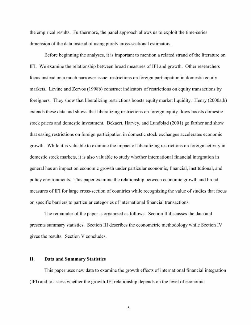
I. Introduction

Theory provides conflicting predictions about the growth effects of international financial

integration (IFI), i.e., the degree to which an economy does not restrict cross-border transactions.

According to some theories, IFI facilitates risk-sharing and thereby enhances production

specialization, capital allocation, and economic growth (Obstfeld, 1994; Acemoglu and Zilibotti,

1997). Further, in the standard neoclassical growth model, IFI eases the flow of capital to capital-

scarce countries with positive output effects. Also, IFI may enhance the functioning of domestic

financial systems, through the intensification of competition and the importation of financial

services, with positive growth effects (Klein and Olivei, 2000; Levine, 2001). On the other hand,

IFI in the presence of pre-existing distortions can actually retard growth.1 Boyd and Smith (1992),

for instance, show that IFI in countries with weak institutions and policies – e.g., weak financial and

legal systems – may actually induce a capital outflow from capital-scarce countries to capital-

abundant countries with better institutions. Thus, some theories predict that international financial

integration will promote growth only in countries with sound institutions and good policies.

Although theoretical disputes and the concomitant policy debate over the growth effects of

IFI have produced a burgeoning empirical literature, resolving this issue is complicated by the

difficulty in measuring IFI. Countries impose a complex array of price and quantity controls on a

broad assortment of financial transactions. Thus, researchers face enormous hurdles in measuring

cross-country differences in the nature, intensity, and effectiveness of barriers to international

capital flows (Eichengreen, 2001).

1 To paraphrase Eichengreen’s (2001, p.1) insightful literature review, there are innumerable constellations of distortions for which liberalization of international capital controls will hurt resource allocation and growth. For example, in the presence of trade distortions, capital account liberalization may induce capital inflows to sectors in which the country has a comparative disadvantage.

2

In practice, empirical analyses use either (i) proxies for government restrictions on capital

flows or (ii) measures of actual international capital flows. The International Monetary Fund’s

(IMF) IMF-restriction measure is the most commonly used proxy of government restrictions on

international financial transactions. It classifies countries on an annual basis by the presence or

absence of restrictions, i.e., it is a zero-one dummy variable. Quinn (1997) attempts to improve

upon the IMF-restriction measure by reading through the IMF’s narrative descriptions of capital

account restrictions and assigning scores of the intensity of capital restrictions. Unfortunately, the

Quinn (1997) measure is only available for intermittent years for most countries (1958, 1973, 1982,

and 1988). The advantage of the IMF-Restriction and Quinn (1997) measures is that they proxy

directly for government impediments. The disadvantage of both measures, as noted above, stems

from the difficulty in accurately gauging the magnitude and effectiveness of government

restrictions.

Empirical studies also use measures of actual international capital flows to proxy for

international financial openness. The assumption is that more capital flows as a share of Gross

Domestic Product (GDP) are a signal of greater IFI. The advantage of these measures is that they

are widely available and they are not subjective measures of capital restrictions. A disadvantage is

that many factors influence capital flows. Indeed, growth may influence capital flows and policy

changes may influence both growth and capital flows, producing a spurious, positive relationship

between growth and capital flows, and growth may affect capital flows. This highlights the need to

account for possible endogeneity in assessing the growth IFI-relationship.

Empirical evidence yields conflicting conclusions about the growth effects of IFI. Grilli and

Milesi-Ferretti (1995), Rodrik (1998), and Kraay (1998) find no link between economic growth and

the IMF-restriction measure. In contrast, Edwards (2001) finds that the IMF-restriction measure is

3

negatively associated with growth in rich countries but positively associated with growth in poor

countries. He thus argues that good institutions are necessary to enjoy the positive growth effects of

IFI. Arteta, Eichengreen, and Wyplosz (2001), however, argue that Edwards’s results are not robust

to small changes in the econometric specification. While Quinn (1997) finds that his measure of

capital account openness is positively linked with growth, Arteta, Eichengreen, and Wyplosz (2001)

and Kraay (1998) find these results are not robust. Finally, while some studies find that foreign

direct investment (FDI) inflows are positively associated with economic growth when countries are

sufficiently rich (Blomstrom, Lipsey, and Zejan, 1994), educated (Borenzstein, De Gregorio, and

Lee, 1998), or financially developed (Alfaro et al., 2001), Carkovic and Levine (2002) find that

these results are not robust to controlling for simultaneity bias.2

In light of the current state of the literature on the growth effects of IFI, we contribute to

existing empirical analyses in four ways.

First, we examine an extensive array of IFI indicators. We examine the IMF-restriction

measure and the Quinn measure of capital account restrictions. Furthermore, we examine various

measures of capital flows: FDI, portfolio, and total capital flows. Moreover, we consider measures

of just capital inflows as well as measures of total capital flows (inflows plus outflows) to proxy for

IFI because openness is defined both in terms of receiving foreign capital and in terms of domestic

residents having the ability to diversity their investments abroad. We examine a wide array of IFI

proxies because each indicator has advantages and disadvantages.

Second, we examine two new measures of IFI. Lane and Milesi-Ferretti (2002) carefully

compute the accumulated stock of foreign assets and liabilities for an extensive sample of countries.

2 For more detailed literature reviews of cross-country studies of the causes and effects of IFI, see Eichengreen (2001) and Edison, Klein, Ricci, and Sløk (2002). For a review of country-specific experiences with IFI, see Cooper (1999).

4

Since we want to measure the average level of openness over an extended period of time, these

stock measures provide a useful additional indicator. Furthermore, these stock measures are less

sensitive to short-run fluctuations in capital flows associated with factors that are unrelated to IFI,

and may therefore provide a more accurate indicator of IFI than capital flow measures. As proxies

for IFI, we examine both the accumulated stock of liabilities (as a share of GDP) and the

accumulated stock of liabilities and assets (as a share of GDP). Also, we break down the

accumulated stocks of financial assets and liabilities into FDI, portfolio, and total financial claims in

assessing the links between economic growth and a wide assortment of IFI indicators. Thus, we

add these additional IFI indicators to the empirical examination of growth and international

financial integration.

Third, since theory and some past empirical evidence suggest that IFI will only have positive

growth effects under particular institutional and policy regimes, we examine an extensive array of

interaction terms. Specifically, we examine whether IFI is positively associated with growth when

countries have well-developed banks, well-developed stock markets, well functioning legal systems

that protect the rule of law, low levels of government corruption, sufficiently high levels of real per

capita GDP, high levels of educational attainment, prudent fiscal balances, and low inflation rates.

Thus, we search for economic, financial, institutional, and policy conditions under which IFI boosts

growth.

Fourth, we use newly developed panel techniques that control for (i) simultaneity bias, (ii)

the bias induced by the standard practice of including lagged dependent variables in growth

regressions, and (iii) the bias created by the omission of country-specific effects in empirical studies

of the IFI-growth relationship. Since each of these econometric biases is a serious concern in

assessing the growth-IFI nexus, applying panel techniques enhances the confidence we can have in

5

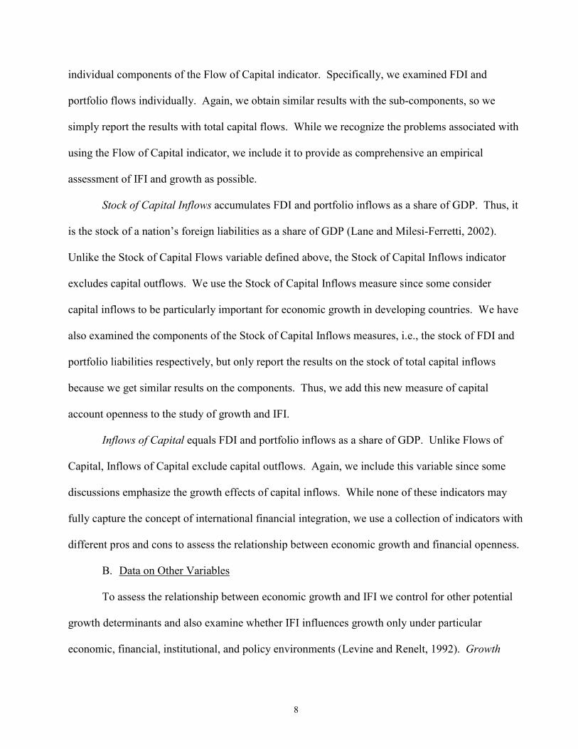
the empirical results. Furthermore, the panel approach allows us to exploit the time-series

dimension of the data instead of using purely cross-sectional estimators.

Before beginning the analyses, it is important to mention a related strand of the literature on

IFI. We examine the relationship between broad measures of IFI and growth. Other researchers

focus instead on a much narrower issue: restrictions on foreign participation in domestic equity

markets. Levine and Zervos (1998b) construct indicators of restrictions on equity transactions by

foreigners. They show that liberalizing restrictions boosts equity market liquidity. Henry (2000a,b)

extends these data and shows that liberalizing restrictions on foreign equity flows boosts domestic

stock prices and domestic investment. Bekaert, Harvey, and Lundblad (2001) go farther and show

that easing restrictions on foreign participation in domestic stock exchanges accelerates economic

growth. While it is valuable to examine the impact of liberalizing restrictions on foreign activity in

domestic stock markets, it is also valuable to study whether international financial integration in

general has an impact on economic growth under particular economic, financial, institutional, and

policy environments. This paper examine the relationship between economic growth and broad

measures of IFI for large cross-section of countries while recognizing the value of studies that focus

on specific barriers to particular categories of international financial transactions.

The remainder of the paper is organized as follows. Section II discusses the data and

presents summary statistics. Section III describes the econometric methodology while Section IV

gives the results. Section V concludes.

II. Data and Summary Statistics

This paper uses new data to examine the growth effects of international financial integration

(IFI) and to assess whether the growth-IFI relationship depends on the level of economic

6

development, financial development, institutional development, or macroeconomic policies. Given

existing barriers to measuring IFI confidently for a broad cross-section of countries, this paper seeks

to improve the analysis of IFI and growth by (i) assessing a broader array of IFI indicators than any

previous study and (ii) using a new type of financial openness indicator. The new indicators are

based on the Lane and Milesi-Ferretti (2002) measures of the accumulated stock of foreign assets

and liabilities.

A. Data on International Financial Integration3

IMF-Restriction: The IMF-Restriction measure equals one in years where there are

restrictions on capital account transactions and zero in years where the are no restrictions on these

external transactions. The data are from the IMF’s Annual Report on Exchange Arrangements and

Exchange Restrictions (AREAER) (line E.2). When conducting regressions averaged over, for

example, the 1980-2000 period, we follow the literature and average the IMF-Restriction measure

over the entire period and use this to measure the average level of openness during the period (e.g.,

see Grilli and Milesi-Ferretti, 1995; Rodrik, 1998; and Klein and Olivei, 2001).4 As emphasized

above, the IMF-Restriction measure may not accurately capture the magnitude and effectiveness of

restrictions on capital flows.

Quinn measure: Based on descriptive information in the in the AREAER, Quinn (1997)

assigns scores associated of the intensity of official restrictions on both capital inflows and

outflows. This measure attempts to improve upon the IMF-Restriction measure by providing

3 The Data Appendix Data provides more detailed information on the variables used in this paper. 4 In 1997, however, there was structural break in the AREAER documentation of capital controls. No longer are countries categorized as having open or restricted capital accounts. Since 1997, information is provided on thirteen separate categories of capital flows, including a distinction between restrictions on inflows and outflows. Because of the structural break, we only use information on IMF-Restriction through 1996.

7

information about the magnitude of restrictions, rather than simply designating countries as closed

or open. The Quinn measure, however, is a particularly subjective measure. Also, it is highly

correlated (0.9) with the IMF-Restriction measure (Edison, Klein, Ricci, and Sløk, 2002).

Moreover, for non-OECD countries, it is only available for two years (1982, 1988) over the sample

period that we examine. Thus, we cannot use the Quinn measure in our panel estimates. Since the

use of panel estimates to reduce statistical biases is an important contribution of this paper, we

confirm our pure cross-country, ordinary least squares (OLS) results using the Quinn measure but

do not report these results in the tables.

Stock of Capital Flows accumulates FDI and portfolio inflows and outflows as a share of

GDP. Thus, it is the stock of a nation’s foreign assets plus liabilities as a share of GDP (Lane and

Milesi-Ferretti, 2002). We examine assets plus liabilities because theoretical concepts of openness

include both (i) the ability of foreigners to invest in a country and (ii) the ability of residents to

invest abroad. We have also examined the components of the Stock of Capital Flows measures, i.e.,

the accumulated stock of FDI and portfolio flows respectively. Since we obtain the same results

with these components, we focus on the stock of total capital inflows and outflows. This is the first

time these stock measures of IFI have been used to study economic growth. The advantage of the

stock measure is that it accumulates flows over a long period. Thus, unlike standard capital flow

measures, the stock measure does not vary very much with short-run changes in the political and

policy climate.

Flow of Capital equals FDI and portfolio inflows and outflows as a share of GDP. Thus, it

is total capital inflows plus outflows divided by GDP. Kraay (1998) used this indicator to measure

capital account openness. As noted, it is important to measure both inflows and outflows in

creating an IFI proxy. As with the Stock of Capital Flows measure, we have examined the

8

individual components of the Flow of Capital indicator. Specifically, we examined FDI and

portfolio flows individually. Again, we obtain similar results with the sub-components, so we

simply report the results with total capital flows. While we recognize the problems associated with

using the Flow of Capital indicator, we include it to provide as comprehensive an empirical

assessment of IFI and growth as possible.

Stock of Capital Inflows accumulates FDI and portfolio inflows as a share of GDP. Thus, it

is the stock of a nation’s foreign liabilities as a share of GDP (Lane and Milesi-Ferretti, 2002).

Unlike the Stock of Capital Flows variable defined above, the Stock of Capital Inflows indicator

excludes capital outflows. We use the Stock of Capital Inflows measure since some consider

capital inflows to be particularly important for economic growth in developing countries. We have

also examined the components of the Stock of Capital Inflows measures, i.e., the stock of FDI and

portfolio liabilities respectively, but only report the results on the stock of total capital inflows

because we get similar results on the components. Thus, we add this new measure of capital

account openness to the study of growth and IFI.

Inflows of Capital equals FDI and portfolio inflows as a share of GDP. Unlike Flows of

Capital, Inflows of Capital exclude capital outflows. Again, we include this variable since some

discussions emphasize the growth effects of capital inflows. While none of these indicators may

fully capture the concept of international financial integration, we use a collection of indicators with

different pros and cons to assess the relationship between economic growth and financial openness.

B. Data on Other Variables

To assess the relationship between economic growth and IFI we control for other potential

growth determinants and also examine whether IFI influences growth only under particular

economic, financial, institutional, and policy environments (Levine and Renelt, 1992). Growth

9

equals real per capita GDP growth, which is computed over the period of analysis. Thus, in the

pure cross-country regressions and in the Table 1 summary statistics Growth is computed over the

1980-2000 period. As is common in cross-country growth regressions, we control for initial

conditions. Initial Income equals the logarithm of real per capita GDP in the initial year of the

period under consideration, and Initial Schooling equals the logarithm of the average years of

secondary schooling in the initial year of the period under consideration. We examine both

financial intermediary development and the liquidity of the domestic stock market. Private Credit

equals the logarithm of credit to the private sector by deposit money banks and other financial

institutions as a share of GDP, while Stock Activity equals the logarithm of the total value of

domestic stock transactions on domestic exchanges as a share of GDP. We use logarithms to reduce

the influence of large outliers of the finance variables. Including the finance variables in levels still

produces a positive relationship between financial development and growth (Levine and Zervos,

1998a). We also control for macroeconomic policies. Inflation equals the growth rate of the

consumer price index and Government Balance equals the governments fiscal balance divided by

GDP, with positive values signifying a surplus and negative values a fiscal deficit. Finally, we

examine the level of institutional development, as measured by the law and order tradition (Law and

Order Tradition) of the country and the level of government corruption (Corruption in

Government), where larger values signify better institutions, i.e., a better law and order tradition and

less corruption.

C. Summary Statistics

Table 1 provides summary statistics. Four key points are worth emphasizing before we

undertake a systematic examination of the IFI-growth relationship.

10

First, rich countries tend to be more open. As shown in Table 1, Panel B, there is a

significant positive correlation between Initial Income and Stock of Flows, Stock of Inflows, Flows

of Capital, and Inflows of Capital. Similarly, these measures of IFI are also positively associated

with Initial Schooling in 1980. The IMF-Restriction measure, however, is not significantly

correlated with income or schooling. Rich, well-educated countries tend to be more open to

international financial transactions, as measured by the stock and flow of capital flows, than poorer

countries and countries with less well-educated workers.

Second, countries with well-developed financial intermediaries, stock markets, legal

systems, and low levels of government corruption tend to have greater capital account openness.

Specifically, Private Credit, Stock Activity, Law and Order, and Corruption are all positively

associated with the measures of Stock of Capital Flows, Stock of Capital Inflows, Flows of Capital,

and Inflows of Capital and negatively associated with the IMF-Restriction measure. Thus, while

measures of IFI are generally unrelated to macroeconomic policies, as proxied by Inflation and the

Government Balance, IFI is strongly correlated with measures of institutional and financial

development.

Third, the IMF-Restriction measure is significantly, negatively correlated with the stock and

flow measures of capital account openness. Specifically, countries that have had a large number of

years over the post-1980 period with capital account restrictions (high values of the IMF-Restriction

measure) have, on average, lower values of Stock of Capital Flows, Stock of Capital Inflows, Flows

of Capital, and Inflows of Capital. Thus, measures of government restrictions on capital account

transactions are negatively linked with international capital flows and the accumulated stock of

those flows.

11

Fourth, the correlations between economic growth and the indicators of IFI are mixed. The

IMF-Restriction measure, Stock of Capital Flows, and Flows of Capital are not significantly

correlated with economic growth at the 0.05 level. However, growth is significantly positively

associated with Stock of Capital Inflows and Inflows of Capital. This suggests the value of

examining a range of indicators and studying IFI indicators that focus on capital inflows.

III. Methodology

This section describes three econometric methods that we use to assess the relationship

between IFI and economic growth. We first use simple ordinary least squares (OLS) regressions

with one observation per country over the 1980-2000 period. Second, we use a two-stage least

squares instrumental variable estimator within the purely cross-country context, i.e., while using

one observation per country over the 1980-2000 period. Third, we use a generalized method of

moments (GMM), dynamic panel procedure to control for potential biases associated with the

purely cross-sectional estimators.

A. OLS framework

The pure cross-sectional, OLS analysis uses data averaged over 1980-2000, such that there

is one observation per country, and heteroskedasticity-consistent standard errors. The basic

regression takes the form:

GROWTH = α + βIFI + γ‘X + εi, (1)

where the dependent variable, GROWTH, equals real per capita GDP growth, IFI is one of the five

measures of international financial integration discussed above, and X represents a matrix of

control variables. We focus on the 1980-2000 period because we have complete data for the 57

countries over this period. When using data in 1960s and 1970s, some countries are missing data

12

over certain periods. Twenty years of data allows us to abstract from business-cycle fluctuations

and short-run political and financial shocks and focus on long-run growth. Thus, as discussed in the

Introduction, some theories suggest that greater international financial integration will be positively

associated with economic growth, i.e., these theories predict that β will be significantly greater than

zero.

We also use a slight variant of equation (1) to examine whether IFI influences growth only

under certain economic, institutional, and policy conditions. Specifically, we also examine the

following regression equation with interaction terms.

GROWTH = α + βIFI + δ[IFI*x] + γ‘X + εi, (1’)

where x is a variable included in the matrix of control variables X. For example, if x is the Rule of

Law, equation (1’) permits us to assess whether international financial integration has a different

influence on growth in countries with high values of the Rule of Law than in countries with low

values of the Rule Law. Specifically, differentiate equation (1’) with respect to IFI to obtain,

∂GROWTH/∂IFI = β + δ*x

If δ>0, this would imply that greater international financial integration has a bigger, positive growth

effect in countries with high levels of x. Thus, for example, the theoretical model developed by

Boyd and Smith (1992) predicts that IFI will positively influence economic performance only in

countries with high levels of the Rule of Law and well-developed financial systems. This model,

therefore, predicts that when x is the Rule of Law or a measure of financial development that δ will

be greater than zero. We examine many “x”’s, i.e., we examine many possible economic,

institutional, and policy conditions that may influence the IFI-growth relationship.

13

B. Two-Stage Least Squares

We also use a two-stage least squares instrumental variable estimator to control for

simultaneity bias while allowing for heteroskedasticity-consistent errors. It uses the same countries,

estimation period, and equation specification as the OLS estimator. With the two-stage least

squares estimator, we also examine whether IFI’s influence on growth depends on other economic,

institutional, and policy conditions. That is, we use also interaction terms in the instrumental

variable regressions.

We use two sets of instrumental variables. First, we use exogenous indicators that past

studies have shown are good predictors of “policy openness” (broadly defined). Specifically, La

Porta, Lopez-de-Silanes, Shleifer, and Vishny (1999) show that legal traditions differ in terms of the

priority they attach to private property rights relative to the power of the state and that legal systems

that emphasize the power of the state tend to be less open to competition. According to this view,

the English common law evolved to protect private property owners against the crown. This

facilitated the ability of private property owners to transact confidently, with positive repercussions

on free, competitive markets. In contrast the French and German civil codes in the 19th century

were constructed to solidify State power. Over time, State dominance produced legal traditions that

focus more on the power of the State and less on the rights of individual investors. Countries with a

socialist legal tradition further reflect these differences. As documented by La Porta et al. (1999),

socialist legal origin countries tend to restrict open, competitive markets. According to the La Porta

et al (1999) theory, these legal traditions spread throughout the world through conquest,

colonization, and imitation, so differences in legal origin can be treated as relatively exogenous.

There are five possible legal origins: English Common Law, French Civil Law, German Civil Law,

Scandinavian Civil Code, and Socialist/Communist law. Thus, we include dummy variables for

14

each country’s legal origin (except the Scandinavian law countries) as instrumental variables.

Second, leading economists, historians, and bio-geographers emphasize the impact of geography on

economic institutions and policies (e.g., Engerman and Sokoloff, 1997). Lands with high rates of

disease and poor agricultural yields – such as the tropics – tend to create political institutions that

are closed to competition and free markets so that the elite can exploit the rest of the population

(See, Acemoglu, Johnson, and Robinson, 2001; Easterly and Levine, 2002). In contrast, countries

with better geographical endowments tend to create political institutions that place greater emphasis

on private property rights and competitive markets in part because the elite benefit more from free

markets than from limiting competition and exploiting domestic labor. We use the absolute value

of latitudinal distance from the equator as an additional instrument in the two-stage least squares

regressions. C. Motivation for the Dynamic Panel Model

The dynamic panel approach offers advantages to OLS and also improves on previous

efforts to examine the IFI-growth link using panel procedures. First, estimation using panel data --

that is pooled cross-section and time-series data – allows us to exploit the time-series nature of the

relationship between IFI and growth. Second, in a pure cross-country instrumental variable

regression, any unobserved country-specific effect becomes part of the error term, which may bias

the coefficient estimates as we explain in detail below. Our panel procedures control for country-

specific effects. Third, unlike existing cross-country studies, our panel estimator (a) controls for the

potential endogeneity of all explanatory variables and (b) accounts explicitly for the biases induced

by including initial real per capita GDP in the growth regression. Thus, the dynamic panel

estimator is free from some of the biases plaguing past studies of IFI and growth.

15

D. Detailed Presentation of the Econometric Methodology

We use the Generalized-Method-of-Moments (GMM) estimators developed for dynamic

panel data that were introduced by Holtz-Eakin, Newey, and Rosen (1990), Arellano and Bond

(1991), and Arellano and Bover (1995). Our panel consists of data for a maximum of 57 countries

over the period 1976-2000. We average data over non-overlapping, five-year periods, so that data

permitting there are five observations per country (1976-1980, 1981-1985, ..., 1996-2000).5 The

subscript “t” designates one of these five-year averages. Consider the following regression

equation,

y y y Xi t i t i t i t i i t, , , , ,( ) '− = − + + +− −1 11α β η ε (2)

where y is the logarithm of real per capita GDP, X represents the set of explanatory variables (other

than lagged per capita GDP), η is an unobserved country-specific effect, ε is the error term, and the

subscripts i and t represent country and time period, respectively. Specifically, X includes an IFI

indicator as well as other possible growth determinants. We also use time dummies to account for

period-specific effects, though these are omitted from the equations in the text. We can rewrite

equation (2).

y y Xi t i t i t i i t, , , ,'= + + +−α β η ε 1 (3)

To eliminate the country-specific effect, take first-differences of equation (3).

( ) ( ) ( )y y y y X Xi t i t i t i t i t i t i t i t, , , , , , , ,'− = − + − + −− − − − −1 1 2 1 1α β ε ε

5 For each five-year period, we require that a country has three years of non-missing data for that variable or the variable is set to missing. We include the early period in the panel estimation, 1976-1980, which is excluded from the pure cross-section results, because we need as many time periods as possible to have confidence in the dynamic panel estimation. For this initial period, about 25 percent of the countries have missing data.

16

The use of instruments is required to deal with (1) the endogeneity of the explanatory variables,

and, (2) the problem that by construction the new error term ε εi t i t, ,− −1 is correlated with the

lagged dependent variable, y yi t i t, ,− −−1 2 . Under the assumptions that (a) the error term is not

serially correlated, and (b) the explanatory variables are weakly exogenous (i.e., the explanatory

variables are uncorrelated with future realizations of the error term), the GMM dynamic panel

estimator uses the following moment conditions:

( )[ ]E y for s t Ti t s i t i t, , , ; , ...,− −⋅ − = ≥ =ε ε 1 0 2 3 (4)

( )[ ]E X for s t Ti t s i t i t, , , ; , ...,− −⋅ − = ≥ =ε ε 1 0 2 3 (5)

We refer to the GMM estimator based on these conditions as the difference estimator.

There are, however, conceptual and statistical shortcomings with this difference estimator.

Conceptually, we would also like to study the cross-country relationship between financial

development and per capita GDP growth, which is eliminated in the difference estimator.

Statistically, Alonso-Borrego and Arellano (1996) and Blundell and Bond (1997) show that when

the explanatory variables are persistent over time, lagged levels make weak instruments for the

regression equation in differences. Instrument weakness influences the asymptotic and small-

sample performance of the difference estimator. Asymptotically, the variance of the coefficients

rises. In small samples, weak instruments can bias the coefficients.

To reduce the potential biases and imprecision associated with the usual estimator, we use a

new estimator that combines in a system the regression in differences with the regression in levels

[Arellano and Bover’s 1995 and Blundell and Bond 1997]. The instruments for the regression in

differences are the same as above. The instruments for the regression in levels are the lagged

differences of the corresponding variables. These are appropriate instruments under the following

additional assumption: although there may be correlation between the levels of the right-hand side

17

variables and the country-specific effect in equation (3), there is no correlation between the

differences of these variables and the country-specific effect, i.e.,

[ ] [ ]

[ ] [ ]E y E y

and E X E X for all p and q

i t p i i t q i

i t p i i t q i

, ,

, ,

+ +

+ +

⋅ = ⋅

⋅ = ⋅

η η

η η (6)

The additional moment conditions for the second part of the system (the regression in levels) are:

( ) ( )[ ]E y y for si t s i t s i i t, , ,− − −− ⋅ + = =1 0 1η ε (7)

( ) ( )[ ]E X X for si t s i t s i i t, , ,− − −− ⋅ + = =1 0 1η ε (8)

Thus, we use the moment conditions presented in equations (4), (5), (7), and (8), use instruments

lagged two period (t-2), and employ a GMM procedure to generate consistent and efficient

parameter estimates.6,7

Consistency of the GMM estimator depends on the validity of the instruments. To address

this issue we consider two specification tests suggested by Arellano and Bond (1991), Arellano and

Bover (1995), and Blundell and Bond (1997). The first is a Sargan test of over-identifying

6 We use a variant of the standard two-step system estimator that controls for heteroskedasticity. Typically, the system estimator treats the moment conditions as applying to a particular time period. This provides for a more flexible variance-covariance structure of the moment conditions because the variance for a given moment condition is not assumed to be the same across time. This approach has the drawback that the number of overidentifying conditions increases dramatically as the number of time periods increases. Consequently, this typical two-step estimator tends to induce over-fitting and potentially biased standard errors, which is particularly important for this paper because of data limitations. To limit the number of overidentifying conditions, we follow Calderon, Chong and Loayza (2000) and apply each moment condition to all available periods. This reduces the over-fitting bias of the two-step estimator. However, applying this modified estimator reduces the number of periods by one. While in the standard estimator time dummies and the constant are used as instruments for the second period, this modified estimator does not allow the use of the first and second period. We confirm the results using the standard system estimator. 7 Recall that we assume that the explanatory variables are “weakly exogenous.” This means they can be affected by current and past realizations of the growth rate but not future realizations of the error term. Weak exogeneity does not mean that agents do not take into account expected future growth in their decision to undertake IFI; it just means that unanticipated shocks to future growth do not influence current IFI. We statistically assess the validity of this assumption.

18

restrictions, which tests the overall validity of the instruments by analyzing the sample analog of the

moment conditions used in the estimation process. The second test examines the hypothesis that the

error term ε i t, is not serially correlated. In both the difference regression and the system

difference-level regression we test whether the differenced error term is second-order serially

correlated (by construction, the differenced error term is probably first-order serially correlated even

if the original error term is not).

IV. Results

A. International Financial Integration and Economic Growth

Using the econometric methods outlined above, this section presents regression results

concerning the relationship between economic growth and various measures of IFI and also assesses

whether the growth-IFI relationship depends on economic, financial, institutional, and policy factors

as suggested by some theories.

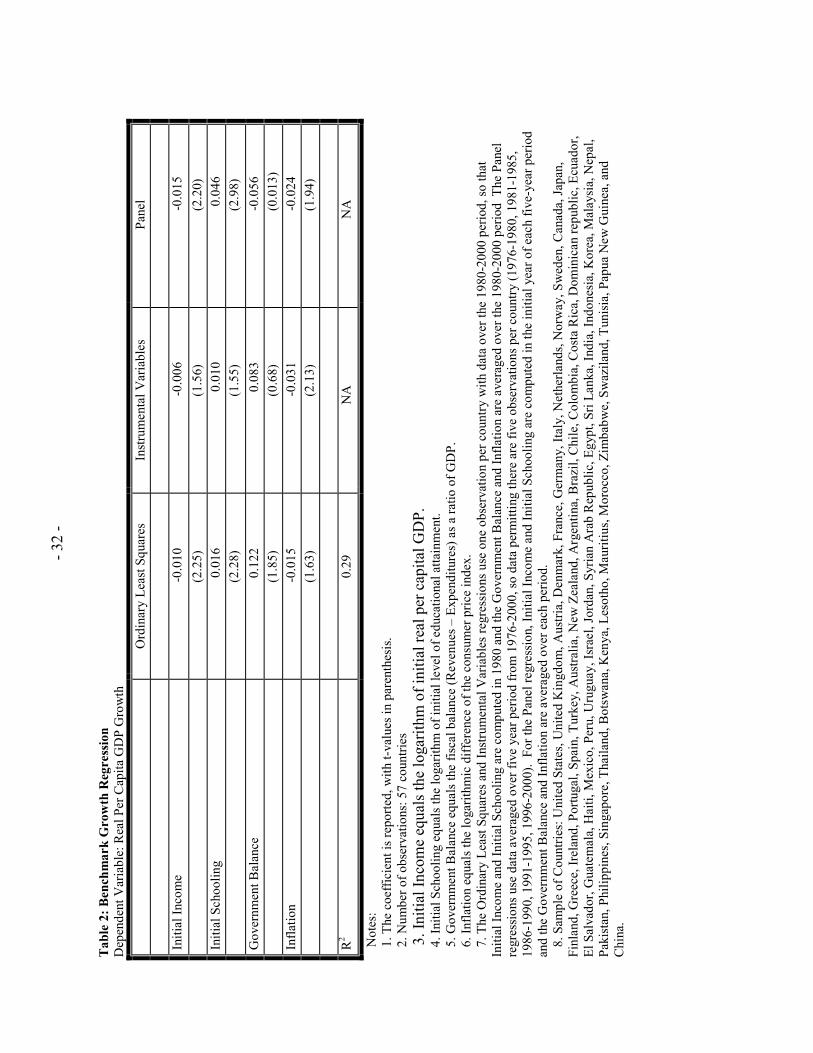
Table 2 presents the benchmark regression without any IFI proxies. Specifically, the

regressions simply include the logarithm of initial real per capita GDP, the logarithm of initial

schooling, the average government fiscal balance over the period, and the average inflation rate

over the period. We present the OLS, instrumental variables (one observation per country) and the

GMM system panel estimator (five observations per country) regressions.

The Table 2 OLS results are consistent with previous cross-country growth regressions. The

logarithm of initial income enters significantly and negatively, which is evidence of conditional

convergence. We also find that the logarithm of initial schooling is significant and positive,

suggesting a positive relationship between educational attainment of the workforce and future

economic growth. The macroeconomic policy indicators, the government balance and inflation

19

enter with the expected signs. While fiscal surplus and inflation enter the growth equation jointly

significantly, neither enters individually significantly in the OLS regression; it is difficult to identify

the independent impact of the fiscal surplus and the rate of inflation on economic growth.

The benchmark regression results are broadly consistent across the three econometric

methodologies. The two-stage least squares regression results produce the same sign as the OLS

regressions. While the logarithm of initial income and the logarithm of initial schooling do not

enter with t-statistics greater than two, inflation is negatively and significantly related to growth in

the two-stage least squares regression.

The system panel estimates further confirm the OLS regressions. The logarithm of initial

income and schooling enter significantly and with the same sign as the OLS regressions. The panel

estimates also suggest a significant, negative relationship between inflation and economic growth.

Unfortunately, when we move to the panel estimator, we lose country observations because some of

the countries do not have sufficient data continuously over the entire 1976-2000 period. We have

40 countries in the Table 2 regression. Importantly, however, the panel estimates pass the

specifications tests defined above. The Sargan test has a p-value of 0.17, which means we do not

reject the econometric specification and the validity of the instruments. Similarly, the serial

correlation test has a p-value of 0.56, which means we do not reject econometric model due to serial

correlation.

Table 3 examines the relationship between economic growth and IFI controlling for the

same benchmark regressors presented in Table 2. We present results on five measures: IMF-

Restriction, the Stock of Capital Flows, Flow of Capital, Stock of Capital Inflows, and Inflow of

Capital. As discussed above, we examined the components of these indicators and obtain similar

results. Thus, Table 3 summarizes the results of 14 regressions, five regressions each for the OLS

20

and two-stage least squares specifications and four regressions for the panel methodology. The

reasons there is one less regression for the panel is that we are unable to use the system panel

estimator for the IMF-Restriction measure because there is too little cross-time variation in this

variable, on average, across the countries and because the IMF-Restriction variable is not available

in the last 5-year period, 1996-2000, as discussed above.

Table 3’s regressions do not suggest a strong relationship between IFI and economic growth.

The IMF-Restriction measure, the Stock of Capital Flows, and the Stock of Capital Inflows are not

significantly related to economic growth in any of the regressions. In the OLS regression, the Flow

of Capital and Inflow of Capital measures are positively associated with growth. In the two-stage

least square regression that controls for the endogeneity of capital flows, however, none of the IFI

measures are significantly associated with growth. This suggests that OLS results may be driven by

reverse causality. Importantly, the instrumental variables do a good job of explaining cross-country

variation in the IFI measures. We reject the null hypothesis that the instruments do not explain the

IFI measures at the 0.01 level in all of the two-stage least squares regressions in Table 3.

The panel estimates in Table 3 suggest that there is a not a robust relationship between IFI

and economic growth.8 There is only one case in which the IFI indicator is significantly associated

with growth, i.e., for the indicator of total capital inflows and outflows as a share of GDP. For

those that have particularly strong priors that the Flows of Capital indicator is better than the other

IFI indicators, these results suggest the IFI exerts a positive influence on economic growth.

However, since the IFI-growth relationship is consistent neither across IFI indicators nor across the

8 The four panel regressions in Table 3 pass the standard specifications tests. Specifically, none reject the Sargan test, i.e., they do not reject the econometric specification and the validity of the instruments. Also, the regressions do not exhibit significant serial correlation, i.e., they do not reject the null hypothesis of no serial correlation as discussed in the methodology section.

21

different estimation procedures, we interpret the econometric results as not strongly rejecting the

null hypothesis of no statistical relationship between IFI and economic growth.

B. IFI Under Different Economic, Financial, Institutional, and Policy Environments

Next, we examine interaction terms to assess whether IFI exerts a positive influence on

growth under certain economic, financial, institutional, and policy environment. Specifically, we

first examine whether the growth effects of IFI depend on the level of GDP per capita or the level of

educational attainment. Second, we examine whether the growth-IFI relationship depends on the

level of financial development, as proxied by banking sector development and stock market

development respectively. Third, we test whether IFI’s growth impact varies with level of

institutional development, as measured by the law and order tradition of the country and the degree

of government corruption. Finally, we study the growth-IFI link under different macroeconomic

policies, as proxied by inflation and the government fiscal surplus. Thus, as discussed above, we

examine the following specification,

GROWTH = α + βIFI + δ[IFI*x] + γx + [the benchmark control variables] + εi,

where x is a variable included in the matrix of control variables X, and is either income per capita,

educational attainment, bank development, stock market development, the Rule of Law,

government corruption, inflation, or the fiscal balance. In Tables 4-7, we report the estimated

coefficients on IFI, the interaction term, and x, i.e., we report statistics on β, δ, and γ. For brevity,

we simply present the OLS result because the two-stage least squares and panel regression results

are very similar.

Contrary to some theories and past empirical evidence, Table 4 indicates that international

financial integration does not exert a positive influence on growth in countries with suitably high

levels of GDP per capita or sufficiently high levels of educational attainment. Out of the ten

22

regressions in Table 4, only in the regression where we interact Initial Income with the Stock of

Capital Flows do we find that IFI and the interaction term enter significantly. However, the results

run counter to theory and past findings. In that regression, the results suggest that IFI only

promotes growth in sufficiently poor countries, i.e. the growth effect becomes negative as countries

become sufficiently rich. In sum, we interpret the Table 4 findings as not rejecting the view that IFI

is unrelated to economic growth even when allowing this relationship to vary under different

economic conditions, as measured by GDP per capita and educational attainment.

Similarly, Table 5 shows that international financial integration does not exert a positive

influence on growth in countries with high levels of bank or stock market development. While

banking sector development enters all of the growth regressions positively and significantly

(Levine, Loayza, and Beck, 2000), the IFI indicator and the interaction terms between IFI and the

financial development indicators never enter significantly. Again, these findings do not show that

IFI is unimportant for growth. Rather, the results do not reject the null hypothesis that IFI is

unrelated to economic growth even when allowing this relationship to vary with financial

development.

We do not find statistical support for the view that the growth effects of international

financial integration increase with greater institutional development (Table 6). We examine the

Rule of Law and Corruption, where higher values imply greater adherence to the rule of law and

less government corruption. In three out of the ten regressions, we find that IFI is positively related

to growth when controlling for institutional development and including interaction terms. However,

those regressions the interaction term enters with a sign that runs counter to theoretical predictions.

Specifically, the regressions suggest that while IFI is positively related with growth, the positive

growth-effects diminish as adherence to the rule of law and the integrity of the government

23

increase. Given the infrequency with which the IFI terms enter significantly and the counter-

intuitive results on the interaction terms in those three regressions, we interpret the results as not

rejecting the view that IFI is unrelated to economic growth even when allowing this relationship to

vary with institutional development.

Finally, we examine whether the growth-IFI relationship varies with macroeconomic

policies. We use inflation and the government fiscal surplus as measures of macroeconomic

policies. Again, we do not find strong evidence for the view that IFI has a positive growth effect

only in countries with sound macroeconomic policies. IFI enters significantly and positively in only

three out of the ten regressions in Table 7 and in these three regressions, the interaction term does

not enter significantly. Since we control for macroeconomic policies in the Table 3 regressions

(which do not include interaction terms), the Table 7 results do not support the view the IFI boosts

growth in general. Turning to the interaction term, the IFI-fiscal balance interaction term does not

enter significantly in any of the equations (Table 7). In the inflation regressions, the IFI-inflation

term enters significantly in two out of the five regressions. For these equations, the results suggest

that IFI in high inflation regimes has a negative growth effect, i.e., IFI is particularly conducive to

growth in low inflation countries. While these regressions offer some support to the view that the

positive growth effects of IFI depend on macroeconomic stability, these findings are not robust

across the different measures of IFI.

V. Conclusions

This paper uses new data and new econometric techniques to investigate the impact of

international financial integration on economic growth and to assess whether the IFI-growth

relationship depends on the level of economic development, educational attainment, financial

24

development, legal system development, government corruption, and macroeconomic policies. We

contribute to the existing literature by (i) using new measures of international financial integration,

(ii) examining an extensive array of IFI indicators, (iii) employing econometric methods that cope

with statistical biases plaguing past studies of the IFI-growth relationship, and (iv) investigating, as

suggested by some theories, whether IFI only has positive growth effects under particular economic,

financial, institutional, and policy regimes. In studying the IFI-growth relationship, the paper

examines up to 57 countries over the last 20-25 years using an assortment of statistical

methodologies.

The data do not support the view that international financial integration per se accelerates

economic growth even when controlling for particular economic, financial, institutional, and policy

characteristics. Note, however, these results do not imply that openness is unassociated with

economic success. Indeed, IFI is positively associated with real per capita GDP, educational

attainment, banking sector development, stock market development, the law and order tradition of

the country, and government integrity (low levels of government corruption). Thus, successful

countries are generally open economies. Rather, this paper finds that IFI is not robustly linked with

economic growth when using a variety of IFI measures and an assortment of econometric

approaches. Similarly, although there are isolated exceptions, we do not reject the null hypothesis

that IFI is unrelated to economic growth even when allowing this relationship to vary with

economic, financial, institutional, and macroeconomic characteristics.

This paper’s findings must be interpreted cautiously. As emphasized in the Introduction,

there are extreme barriers to measuring openness to international financial transactions. There are

many different types of financial transactions, countries impose a complex array of barriers, and the

effectiveness of these barriers varies across countries, time, and type of financial transaction.

25

Although we use new measures of IFI that improve upon past measures and although we use a more

extensive list of IFI measures than past studies, each of these measures may be criticized for not

fully distinguishing international differences in barriers to financial transactions. Given these

qualifications, this paper finds that although international financial integration is associated with

economic success (high levels of GDP per capita and strong institutions), the data do not lend much

support to the view that international financial integration stimulates economic growth.

26

Acknowledgements

The authors wish to thank Tamim Bayoumi, Michael Klein, Phillip Lane, Gian Maria Milesi-Ferreti, and David Robinson for data and helpful comments and Yutong Li and Bennett Sutton for efficient research assistance. The views expressed in this paper are those of the authors and do not necessarily represent those of the IMF or IMF policy. This research was originally conducted as a background paper for Chapter 4 of the October 2001 IMF World Economic Outlook.

27

References Acemoglu, D., S. Johnson, and J. Robinson, 2001. “The colonial origins of comparative

development: an empirical investigation,” American Economic Review, 91,1369-1401. Acemoglu, D., F. Zilibotti, 1997, “Was Prometheus Unbound by chance? Risk Diversification, and

Growth,” Journal of Political Economy, 105, 709-51. Alfaro, L., A. Chanda, S. Kalemli-Ozcan, and S.n Sayek. "FDI and Economic Growth: The Role of

Local Financial Markets." Harvard Business School, Working Paper, 2001, Number 83. Alonso-Borrego, C. and M.Arellano. “Symmetrically Normalised Instrumental Variable Estimation

Using Panel Data,” CEMFI Working Paper No. 9612, September 1996. Arellano, M. and S. Bond. “Some Tests of Specification for Panel Data: Monte Carlo Evidence and

an Application to Employment Equations,” Review of Economic Studies 1991, 58, pp. 277-297.

Arellano, M., and O. Bover. “Another Look at the Instrumental-Variable Estimation of Error-

Components Models,” Journal of Econometrics 1995, 68, pp. 29-52.

Arteta, C., B. Eichengreen, and C. Wyplosz, 2001, “On the Growth Effects of Capital Account Liberalization,” (unpublished; Berkeley: University of California)

Barro, R. J. and J. Lee. “International Measures of Schooling Years and Schooling Quality”, AER

Papers and Proceedings 1996, 86, pp. 218-223. Beck, T., and R. Levine, 2002, “Stock Market, Banks, and Economic Growth: Cross-Country and

Panel Evidence,” University of Minnesota, mimeo. Bekaert, G., C. R. Harvey, and C. Lundblad, 2001, “Does Financial Liberalization Spur Growth?”

NBER Working Paper No. 8245 (Cambridge, Mass.: National Bureau of Economic Research).

Blomstrom, M., Lipsey, R. and M. Zejan, 1994, “What Explains Growth in Developing

Countries?,” National Bureau of Economic Research Working Paper, No. 5057.

Blundell, R. and S. Bond. “Initial Conditions and Moment Restrictions in Dynamic Panel Data Models,” Journal of Econometrics, 1998, 87, pp. 115-43.

Borensztein, E., De Gregorio, J., and J.W. Lee, 1998, How Does Foreign Investment Affect

Growth? Journal of International Economics, 45. Boyd, J. H., and B. D. Smith, 1992, “Intermediation and the Equilibrium Allocation of Investment

Capital: Implications for Economic Development,” Journal of Monetary Economics, 30, 409-432.

28

Calderon, C.; A. Chong, and N. Loayza. “Determinants of Current Account Deficits in Developing

Countries,” World Bank Research Policy Working Paper 2398, July 2000. Carkovic, M. and R. Levine, 2002, Does Foreign Direct Investment Accelerate Economic Growth?”

University of Minnesota Carlson School of Management), mimeo. Cooper, R., 1999, “Should Capital Controls Be Banished?” Brookings Papers on Economic Activity,

1, 89-141. Easterly, W. and R. Levine, 2002, Tropics, germs, and crops. University of Minnesota, mimeo. Edison, H., M. Klein., L. Ricci, and T. Sløk, 2002, “Capital Account Liberalization and Economic

Performance: Survey and Synthesis,” IMF Working Paper No 02/120, (Washington: International Monetary Fund).

Edwards, S., 2001, “Capital Mobility and Economic Performance: Are Emerging Economies

Different?” NBER Working Paper No. 8076 (Cambridge, Mass.: National Bureau of Economic Research).

Eichengreen, B., 2001, “Capital Account Liberalization: What do Cross-Country Studies Tell Us?”

(unpublished; Berkeley: University of California). Engerman, S. and K. Sokoloff, 1997, “Factor endowments, institutions, and differential paths of

growth among new world economies,” In Haber, Stephen (Ed.), How Latin America Fell Behind, Stanford University Press, Stanford CA, pp. 260-304.

Grilli, V. and G. Maria Milesi-Ferreti, 1995, “Economic Effects and Structural Determinants of

Capital Controls,” Staff Papers, Vol. 42 (September), pp. 517–51. Henry, P., 2000a, “Stock Market Liberalization, Economic Reform, and Emerging Market Equity

Prices,” Journal of Finance, Vol. 55 (April), pp. 529–64. Henry, P., 2000b, “Do Stock Market Liberalizations Cause Investment Booms?” Journal of

Financial Economics, 58, 301-334. Holtz-Eakin, D.; Newey, W, and Rosen, H. “Estimating Vector Autoregressions with Panel Data, “

Econometrica, 1990, 56(6), pp. 1371-1395. Klein, M., and G. Olivei, 2000, “Capital Account Liberalization, Financial Depth, and Economic

Growth,” (unpublished; Somerville, Mass.: Tufts University. Kraay, A., 1998, “In Search of the Macroeconomic Effects of Capital Account Liberalization,”

(unpublished; Washington: World Bank).

29

Lane, P., and G. Maria Milesi-Ferretti, forthcoming, “The External Wealth of Nations,” Journal of International Economics.

La Porta, R., F. Lopez-de-Silanes, A. Shleifer, and R. Vishny, 1999, “The Quality of Government,”

Journal of Law, Economics, and Organization, 15, 222-279. Levine, R., 2001, “International Financial Liberalization and Economic Growth,” Review of

International Economic, 9, 688-702. Levine, R., and S. Zervos, 1998a, “Stock Markets, Banks, and Economic Growth,” American

Economic Review, Vol. 88 (June), 537–58. Levine, R., and S. Zervos, 1998b, “Capital Control Liberalization and Stock Market Development,”

World Development, 26, 1169-84. Levine, R., N. Loayza, and T. Beck, 2000, “Financial Intermediation and Growth: Causality and

Causes,” Journal of Financial Economics, 46, 31-77. Levine, R., and D. Renelt, 1992, “A Sensitivity Analysis of Cross-Country Growth Regressions,”

American Economic Review, Vol. 82 (September), pp. 942–63. Obstfeld, M., 1994, “Risk-taking, Global Diversification, and Growth,” American Economic Review

84, 1310-1329. Quinn, D., 1997, “The Correlates of Change in International Financial Regulation,” American

Political Science Review, Vol. 91, (September), pp. 531–51. Rodrik, D., 1998, “Who Needs Capital-Account Convertibility,” (unpublished; Cambridge, Mass.:

Harvard University).

Tab

le 1

. Dat

a D

escr

iptio

n

Pane

l A. S

umm

ary

Stat

istic

s

Var

iabl

e M

ean

St

d.

Dev

.

M

in.

Val

ue

M

ax.

Val

ue

Gro

wth

1

.02

.0

2

-.03

.0

8 In

itial

Inco

me

2 7.

96

.9

9

5.97

9.47

In

itial

Sch

oolin

g3 3.

81

.6

5

2.04

4.65

G

over

nmen

t Bal

ance

4

-.03

.0

3

-.10

.1

0 In

flatio

n ra

te5

.15

.2

2

.02

1.

29

Priv

ate

Cre

dit6

-1.0

0

.82

-3

.21

.5

7 St

ock

Act

ivity

7 -3

.50

1.

81

-8

.09

-.0

2 La

w a

nd O

rder

8 4.

05

1.

36

1.

70

6

Cor

rupt

ion9

4.84

1.20

2.48

6.89

IM

F R

estri

ctio

n10

.74

.3

7

0

1 St

ock

of C

apita

l Flo

ws 1

1 .5

3

.60

.0

1

2.77

Fl

ow o

f Cap

ital 1

2 .0

5

.05

-.0

1

.22

Stoc

k of

Cap

ital I

nflo

ws 1

3 .3

5

.30

.0

1

1.13

In

flow

of C

apita

l 14

.03

.0

2

-.00

.1

2

N

otes

to ta

ble:

1. R

eal p

er c

apita

GD

P gr

owth

rate

(cal

cula

ted

in lo

garit

hmic

term

s)

2.

Log

arith

m o

f Ini

tial r

eal p

er c

apita

l GD

P in

198

0.

3.

Log

arith

m o

f ave

rage

yea

rs o

f sch

oolin

g in

198

0.

4.

Fis

cal B

alan

ce (R

even

ues –

Exp

endi

ture

s) a

s a ra

tio o

f GD

P.

5.

Infla

tion

usin

g co

nsum

er p

rice

inde

x (c

alcu

late

d in

loga

rithm

ic fi

rst d

iffer

ence

term

s).

6.

Log

arith

m o

f priv

ate

cred

it by

dep

osit

mon

ey b

anks

and

oth

er fi

nanc

ial i

nstit

utio

ns a

s a ra

tio to

GD

P

7. L

ogar

ithm

of s

tock

mar

ket t

otal

val

ue tr

aded

as a

ratio

GD

P

8. IC

RG

– L

aw a

nd O

rder

9. IC

RG

– C

orru

ptio

n in

Gov

ernm

ent

10.

Cap

ital A

ccou

nt R

estri

ctio

ns fr

om th

e IM

F A

nnua

l Rep

ort A

REA

ER, a

vera

ge 1

980-

1996

. 1

1. S

tock

of C

apita

l Ass

ets a

nd L

iabi

litie

s div

ided

by

GD

P (a

vera

ge: 1

996

– 19

98, F

DI a

nd P

ortfo

lio).

12.

FD

I plu

s Por

tfolio

inflo

ws a

nd o

utflo

ws d

ivid

ed b

y G

DP

(ave

rage

: 198

0-20

00).

13.

Sto

ck o

f Cap

ital L

iabi

litie

s di

vide

d by

GD

P (a

vera

ge: 1

996

– 19

98, F

DI a

nd P

ortfo

lio).

14.

FD

I and

Por

tfolio

inflo

ws d

ivid

ed b

y G

DP

(ave

rage

: 198

0-20

00).

- 31

-

Pane

l B. C

orre

latio

n M

atri

x

G

row

th

Initi

al

Inco

me

Initi

al

Scho

olin

g G

over

nme

nt B

alan

ce

Infla

tion

IMF

Res

trict

ion

Stoc

k of

C

apita

l Fl

ows

Flow

of

Cap

ital

Stoc

k of

C

apita

l In

flow

s

Inflo

ws o

f C

apita

l Pr

ivat

e C

redi

t St

ock

Act

ivity

La

w a

nd

Ord

er

Cor

rupt

ion

Gro

wth

1.

00

In

itial

Inco

me

-0.1

0 1.

00

Scho

olin

g 0.

24

0.76

* 1.

00

G

over

nmen

t Bal

ance

0.

22

0.05

-0

.02

1.00

In

flatio

n -0

.26*

-0

.00

-0.0

7 -0

.16

1.00

IMF

Res

trict

ion

-0.0

3 -0

.55

-0.4

2 -0

.22

0.14

1.

00

Stoc

k of

Cap

ital F

low

s 0.

07

0.60

* 0.

48*

0.22

-0

.25*

-0

.62*

1.

00

Fl

ow o

f Cap

ital

0.04

0.

54*

0.41

* 0.

21

-0.2

2 -0

.53*

0.

93*

1.00

St

ock

of C

apita

l Inf

low

s 0.

25*

0.55

* 0.

42*

0.24

-0

.23

-0.4

7*

0.77

* 0.

72*

1.00

Inflo

ws o

f Cap

ital

0.29

* 0.

42*

0.32

* 0.

29*

-0.1

7 -0

.36*

0.

62*

0.69

* 0.

92*

1.00

Pr

ivat

e C

redi

t 0.

26*

0.66

* 0.

64*

-0.0

0 -0

.37*

-0

.48*

0.

60*

0.49

* 0.

54*

0.40

* 1.

00

St

ock

Act

ivity

0.

21

0.46

* 0.

46*

0.23

-0

.18

-0.4

1*

0.56

* 0.

49*

0.57

* 0.

51*

0.71

* 1.

00

Law

and

Ord

er

0.26

* 0.

76*

0.59

* 0.

22

-0.2

5 -0

.56*

0.

69*

0.72

* 0.

66*

0.59

* 0.

67*

0.54

* 1.

00

C

orru

ptio

n 0.

10

0.82

* 0.

67*

0.06

-0

.19

-0.4

8*

0.69

* 0.

70*

0.65

* 0.

54*

0.68

* 0.

49*

0.87

* 1.

00

Not

e: S

igni

fican

t coe

ffic

ient

s (at

5 p

erce

nt si

gnifi

canc

e le

vel)

are

deno

ted

by a

*

- 32

-

Tab

le 2

: Ben

chm

ark

Gro

wth

Reg

ress

ion

Dep

ende

nt V

aria

ble:

Rea

l Per

Cap

ita G

DP

Gro

wth

Ord

inar

y Le

ast S

quar

es

Inst

rum

enta

l Var

iabl

es

Pane

l

In

itial

Inco

me

-0.0

10

-0.0

06

-0.0

15

(2

.25)

(1

.56)

(2

.20)

In

itial

Sch

oolin

g 0.

016

0.01

0 0.

046

(2

.28)

(1

.55)

(2

.98)

G

over

nmen

t Bal

ance

0.

122

0.08

3 -0

.056

(1.8

5)

(0.6

8)

(0.0

13)

Infla

tion

-0.0

15

-0.0

31

-0.0

24

(1

.63)

(2

.13)

(1

.94)

R

2 0.

29

NA

N

A

N

otes

:

1. T

he c

oeffi

cien

t is r

epor

ted,

with

t-va

lues

in p

aren

thes

is.

2.

Num

ber o

f obs

erva

tions

: 57

coun

tries

3. In

itial

Inco

me

equa

ls th

e lo

garit

hm o

f ini

tial r

eal p

er c

apita

l GD

P.

4.

Initi

al S

choo

ling

equa

ls th

e lo

garit

hm o

f ini

tial l

evel

of e

duca

tiona

l atta

inm

ent.

5.

Gov

ernm

ent B

alan

ce e

qual

s the

fisc

al b

alan

ce (R

even

ues –

Exp

endi

ture

s) a

s a ra

tio o

f GD

P.

6.

Infla

tion

equa

ls th

e lo

garit

hmic

diff

eren

ce o

f the

con

sum

er p

rice

inde

x.

7.

The

Ord

inar

y Le

ast S

quar

es a

nd In

stru

men

tal V

aria

bles

regr

essi

ons u

se o

ne o

bser

vatio

n pe

r cou

ntry

with

dat

a ov

er th

e 19

80-2

000

perio

d, so

that

In

itial

Inco

me

and

Initi

al S

choo

ling

are

com

pute

d in

198

0 an

d th

e G

over

nmen

t Bal

ance

and

Infla

tion

are

aver

aged

ove

r the

198

0-20

00 p

erio

d T

he P

anel

re

gres

sion

s use

dat

a av

erag

ed o

ver f

ive

year

per

iod

from

197

6-20

00, s

o da

ta p

erm

ittin

g th

ere

are

five

obse

rvat

ions

per

cou

ntry

(197

6-19

80, 1

981-

1985

, 19

86-1

990,

199

1-19

95, 1

996-

2000

). F

or th

e Pa

nel r

egre

ssio

n, In

itial

Inco

me

and

Initi

al S

choo

ling

are

com

pute

d in

the

initi

al y

ear o

f eac

h fiv

e-ye

ar p

erio

d an

d th

e G

over

nmen

t Bal

ance

and

Infla

tion

are

aver

aged

ove

r eac

h pe

riod.

8. S

ampl

e of

Cou

ntrie

s: U

nite

d St

ates

, Uni

ted

Kin

gdom

, Aus

tria,

Den

mar

k, F

ranc

e, G

erm

any,

Ital

y, N

ethe

rland

s, N

orw

ay, S

wed

en, C

anad

a, Ja

pan,

Fi

nlan

d, G

reec

e, Ir

elan

d, P

ortu

gal,

Spai

n, T

urke

y, A

ustra

lia, N

ew Z

eala

nd, A

rgen

tina,

Bra

zil,

Chi

le, C

olom

bia,

Cos

ta R

ica,

Dom

inic

an re

publ

ic, E

cuad

or,

El S

alva

dor,

Gua

tem

ala,

Hai

ti, M

exic

o, P

eru,

Uru

guay

, Isr

ael,

Jord

an, S

yria

n A

rab

Rep

ublic

, Egy

pt, S

ri La

nka,

Indi

a, In

done

sia,

Kor

ea, M

alay

sia,

Nep

al,

Paki

stan

, Phi

lippi

nes,

Sing

apor

e, T

haila

nd, B

otsw

ana,

Ken

ya, L

esot

ho, M

aurit

ius,

Mor

occo

, Zim

babw

e, S

waz

iland

, Tun

isia

, Pap

ua N

ew G

uine

a, a

nd

Chi

na.

- 33

-

Tab

le 3

: Eco

nom

ic G

row

th a

nd In

tern

atio

nal F

inan

cial

Inte

grat

ion

Dep

ende

nt V

aria

ble:

Rea

l Per

Cap

ita G

DP

Gro

wth

Inte

rnat

iona

l Fin

anci

al In

tegr

atio

n M

easu

re

Ord

inar

y L

east

Sq

uare

s In

stru

men

tal V

aria

bles

Pa

nel

IMF

Res

trict

ion

0.00

2 (0

.29)

-0

.011

(0.9

1)

NA

St

ock

of C

apita

l Flo

ws

0.00

3 (0

.72)

0.

008

(0.8

5)

0.00

2 (0

.35)

Fl

ow o

f Cap

ital

0.10

1 (2

.46)

* 0.

056

(0.7

9)

0.07

7 (2

.08)

St

ock

of C

apita

l Inf

low

s 0.

002

(0.2

5)

-0.0

07 (0

.63)

0.

001

(0.0

33)

Inflo

w o

f Cap

ital

0.18

3 (2

.24)

* 0.

078

(0.6

2)

0.13

2 (1

.23)

Not

es:

1.

Num

bers

in p

aren

thes

is a

re t-

stat

istic

s; a

nd *

indi

cate

s sig

nific

ant a

t the

5 p

erce

nt le

vel

2.

The

regr

essi

on a

lso

incl

ude

Initi

al In

com

e, In

itial

Sch

oolin

g, th

e G

over

nmen

t Bal

ance

, and

Infla

tion.

3. C

olum

n 2

pres

ent O

LS re

gres

sion

resu

lts u

sing

het

eros

keda

stic

ity c

onsi

sten

t sta

ndar

d er

rors

.

4. C

olum

n 3

pres

ents

Tw

o-St

age

Leas

t Squ

ares

res

ults

, with

het

eros

keda

stic

ity c

onsi

sten

t sta

ndar

d er

rors

, whe

re th

e in

stru

men

ts a

re th

e la

titud

inal

di

stan

ce fr

om th

e eq

uato

r, an

d a

dum

my

varia

ble

for t

he le

gal o

rigin

of t

he c

ount

ry (C

omm

on, F

renc

h C

ivil,

Ger

man

Civ

il, S

cand

inav

ian,

Soc

ialis

t).

5.

Col

umn

4 pr

esen

ts d

ynam

ic sy

stem

pan

el re

gres

sion

resu

lts w

ith ro

bust

stan

dard

err

ors.

Not

e, w

e ar

e un

able

to u

se th

e sy

stem

pan

el e

stim

ator

for t

he

IMF-

Res

trict

ion

mea

sure

bec

ause

ther

e is

too

little

cro

ss-ti

me

varia

tion

in th

is v

aria

ble,

on

aver

age,

acr

oss t

he c

ount

ries a

nd b

ecau

se th

e IM

F-R

estri

ctio

n va

riabl

e is

not

ava

ilabl

e in

the

last

5-y

ear p

erio

d, 1

996-

2000

, as d

iscu

ssed

in th

e te

xt.

6.

The

Ord

inar

y Le

ast S

quar

es a

nd In

stru

men

tal V

aria

bles

regr

essi

ons u

se o

ne o

bser

vatio

n pe

r cou

ntry

with

dat

a ov

er th

e 19

80-2

000

perio

d, so

that

In

itial

Inco

me

and

Initi

al S

choo

ling

are

com

pute

d in

198

0 an

d th

e G

over

nmen

t Bal

ance

and

Infla

tion

are

aver

aged

ove

r the

198

0-20

00 p

erio

d T

he P

anel

re

gres

sion

s use

dat

a av

erag

ed o

ver f

ive

year

per

iod

from

197

6-20

00, s

o da

ta p

erm

ittin

g th

ere

are

five

obse

rvat

ions

per

cou

ntry

(197

6-19

80, 1

981-

1985

, 19

86-1

990,

199

1-19

95, 1

996-

2000

). F

or th

e Pa

nel r

egre

ssio

n, In

itial

Inco

me

and

Initi

al S

choo

ling

are

com

pute

d in

the

initi

al y

ear o

f eac

h fiv

e-ye

ar p

erio

d an

d th

e G

over

nmen

t Bal

ance

and

Infla

tion

are

aver

aged

ove

r eac

h pe

riod.

5.

The

tabl

e su

mm

ariz

es th

e fin

ding

s fro

m 1

5 se

para

te re

gres

sion

s.

7. IM

F R

estri

ctio

n: C

apita

l Acc

ount

Res

trict

ions

from

the

IMF.

8. S

tock

of C

apita

l Flo

ws:

Sto

ck o

f Cap

ital A

sset

s and

Lia

bilit

ies (

FDI a

nd P

ortfo

lio) d

ivid

ed b

y G

DP.

9. F

low

of C

apita

l: FD

I plu

s Por

tfolio

inflo

ws a

nd o

utflo

ws d

ivid

ed b

y G

DP.

10. S

tock

of C

apita

l Inf

low

s: C

apita

l Lia

bilit

ies(

FDI a

nd P

ortfo

lio) d

ivid

ed b

y G

DP.

11. I

nflo

w o

f Cap

ital:

FDI a

nd P

ortfo

lio in

flow

s div

ided

by

GD

P.

- 34

-

Tab

le 4

: Eco

nom

ic G

row

th a

nd In

tern

atio

nal F

inan

cial

Inte

grat

ion:

Ini

tial E

cono

mic

Con

ditio

ns

Pane

l A. I

nitia

l Inc

ome

Lev

el

Dep

ende

nt V

aria

ble:

Rea

l Per

Cap

ita G

DP

Gro

wth

, 198

0-20

00)

Estim

ated

by

OLS

, Sam

ple

Perio

d 19

80-2

000

Inte

rnat

iona

l Fin

anci

al In

tegr

atio

n M

easu

re

IFI

IFI*

(Ini

tial I

ncom

e)

Initi

al In

com

e IM

F R

estri

ctio

n -0

.002

(0.0

5)

0.00

0 (0

.09)

-0

.01

(2.1

5)*

Stoc

k of

Cap

ital F

low

s 0.

410

(2.5

6)*

-0.0

40 (2

.46)

* -0

.01

(2.0

4)*

Flow

of C

apita

l 0.

079

(0.1

6)

0.00

2 (0

.04)

-0

.01

(3.0

2)*

Stoc

k of

Cap

ital I

nflo

ws

0.01

1 (0

.27)

-0

.001

(0.2

4)

-0.0

1 (2

.18)

* In

flow

of C

apita

l -0

.340

(0.5

5)

0.06

6 (0

.88)

-0

.01

(3.3

4)*

Pane

l B. I

nitia

l Sch

oolin

g D

epen

dent

Var

iabl

e: R

eal P

er C

apita

GD

P G

row

th, 1

980-

2000

Es

timat

ed b

y O

LS, S

ampl

e Pe

riod

1980

-200

0

Inte

rnat

iona

l Fin

anci

al In

tegr

atio

n M

easu

re

IFI

IFI*

(Ini

tial S

choo

ling)

In

itial

Sch

oolin

g IM

F R

estri

ctio

n -0

.010

(0.2

5)

0.00

3 (0

.30)

0.

013

(1.1

6)

Stoc

k of

Cap

ital F

low

s 0.

030

(0.7

5)

-0.0

06 (0

.71)

0.

017

(2.2

6)*

Flow

of C

apita

l 0.

008

(0.0

4)

0.02

3 (0

.43)

0.

014

(1.8

9)

Stoc

k of

Cap

ital I

nflo

ws

0.01

3 (0

.38)

-0

.003

(0.3

4)

0.01

6 (2

.14)

* In

flow

of C

apita

l -0

.140

(0.4

6)

0.08

7 (1

.13)

0.

013

(1.7

7)

Not

es:

1.

Num

bers

in p

aren

thes

is a

re t-

stat

istic

s; a

nd *

indi

cate

s sig

nific

ant a

t the

5 p

erce

nt le

vel

2.

The

regr

essi

on a

lso

incl

ude:

the

loga

rithm

of G

DP

per c

apita

in 1

980,

the

loga

rithm

of t

he se

cond

ary

scho

ol e

nrol

lmen

t rat

e in

198

0, th

e av

erag

e an

nual

CPI

infla

tion

rate

bet

wee

n 19

80-2

000,

and

the

aver

age

annu

al g

over

nmen

t bud

get b

alan

ce fr

om 1

980-

2000

.

3. T

he ta

ble

pres

ents

OLS

regr

essi

on re

sults

usi

ng h

eter

oske

dast

icity

con

sist

ent e

rror

s.

4. T

he ta

ble

sum

mar

izes

the

findi

ngs f

rom

10

sepa

rate

regr

essi

ons.

5.

IMF

Res

trict

ion:

Cap

ital A

ccou

nt R

estri

ctio

ns fr

om th

e IM

F.

6.

Sto

ck o

f Cap

ital F

low

s: S

tock

of C

apita

l Ass

ets a

nd L

iabi

litie

s (FD

I and

Por

tfolio

) div

ided

by

GD

P.

7.

Flo

w o

f Cap

ital:

FDI p

lus P

ortfo

lio in

flow

s and

out

flow

s div

ided

by

GD

P.

8.

Sto

ck o

f Cap

ital I

nflo

ws:

Cap

ital L

iabi

litie

s(FD

I and

Por

tfolio

) div

ided

by

GD

P.

9.

Inflo

w o

f Cap

ital:

FDI a

nd P

ortfo

lio in

flow

s div

ided

by

GD

P.

10

. Ini

tial I

ncom

e: L

ogar

ithm

of I

nitia

l rea

l per

cap

ital G

DP

in 1

980.

11. I

nitia

l Sch

oolin

g: L

ogar

ithm

of a

vera

ge y

ears

of s

econ

dary

scho

olin

g in

198

0.

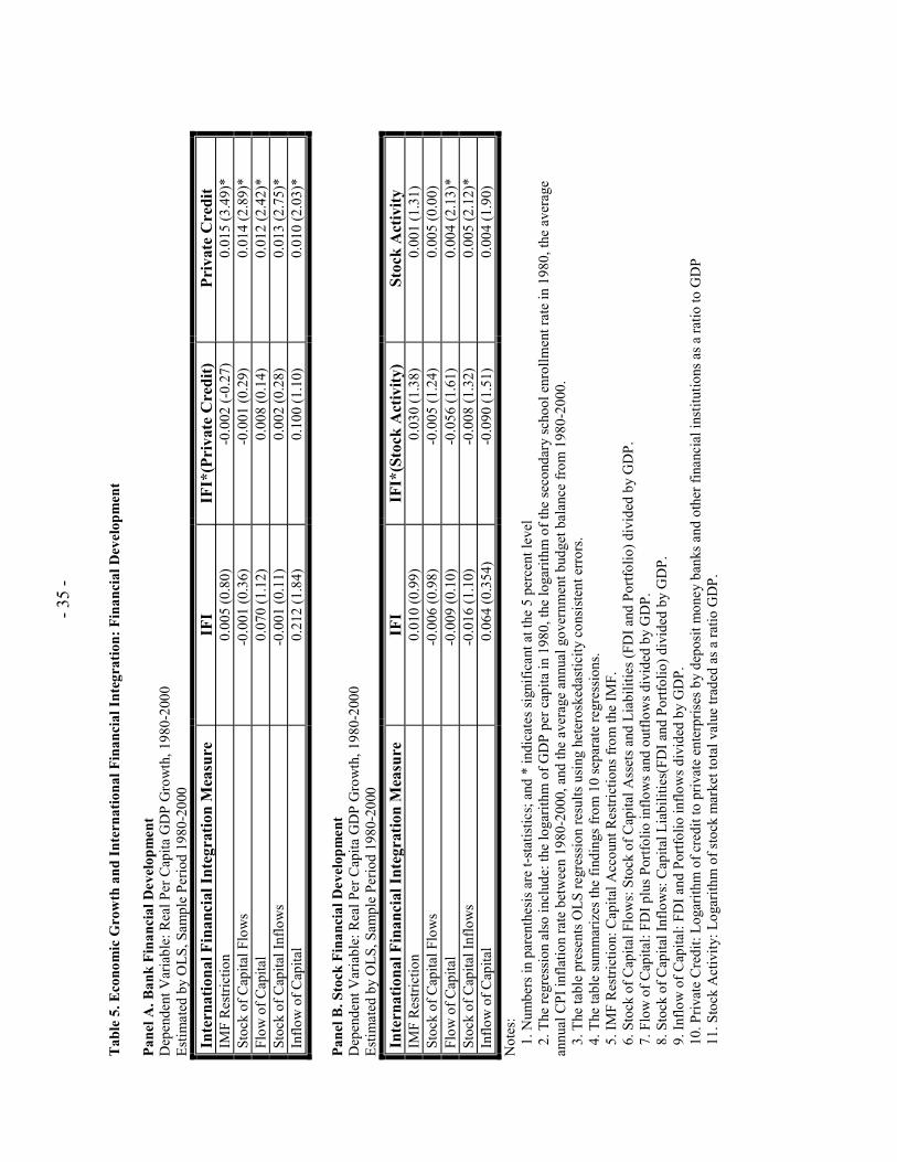
- 35

-

Tab

le 5

. Eco

nom

ic G

row

th a

nd In

tern

atio

nal F

inan

cial

Inte

grat

ion:

Fin

anci

al D

evel

opm

ent

Pane

l A. B

ank

Fina

ncia

l Dev

elop

men

t D

epen

dent

Var

iabl

e: R

eal P

er C

apita

GD

P G

row

th, 1

980-

2000

Es

timat

ed b

y O

LS, S

ampl

e Pe

riod

1980

-200

0

Inte

rnat

iona

l Fin

anci

al In

tegr

atio

n M

easu

re

IFI

IFI*

(Pri

vate

Cre

dit)

Pr

ivat

e C

redi

t IM

F R

estri

ctio

n 0.

005

(0.8

0)

-0.0

02 (-

0.27

) 0.

015

(3.4

9)*

Stoc

k of

Cap

ital F

low

s -0

.001

(0.3

6)

-0.0

01 (0

.29)

0.

014

(2.8

9)*

Flow

of C

apita

l 0.

070

(1.1

2)

0.00

8 (0

.14)

0.

012

(2.4

2)*

Stoc

k of

Cap

ital I

nflo

ws

-0.0

01 (0

.11)

0.

002

(0.2

8)

0.01

3 (2

.75)

* In

flow

of C

apita

l 0.

212

(1.8

4)

0.10

0 (1

.10)

0.

010

(2.0

3)*

Pane

l B. S

tock

Fin

anci

al D

evel

opm

ent

Dep

ende

nt V

aria

ble:

Rea

l Per

Cap

ita G

DP

Gro

wth

, 198

0-20

00

Estim

ated

by

OLS

, Sam

ple

Perio

d 19

80-2

000

Inte

rnat

iona

l Fin

anci

al In

tegr

atio

n M

easu

re

IFI

IFI*

(Sto

ck A

ctiv

ity)

Stoc

k A

ctiv

ity

IMF

Res

trict

ion

0.01

0 (0

.99)

0.

030

(1.3

8)

0.00

1 (1

.31)

St

ock

of C

apita

l Flo

ws

-0.0

06 (0

.98)

-0

.005

(1.2

4)

0.00

5 (0

.00)

Fl

ow o

f Cap

ital

-0.0

09 (0

.10)

-0

.056

(1.6

1)

0.00

4 (2

.13)

* St

ock

of C

apita

l Inf

low

s -0

.016

(1.1

0)

-0.0

08 (1

.32)

0.

005

(2.1

2)*

Inflo

w o

f Cap

ital

0.06

4 (0

.354

) -0

.090

(1.5

1)

0.00

4 (1

.90)

N

otes

:

1. N

umbe

rs in

par

enth

esis

are

t-st

atis

tics;

and

* in

dica

tes s

igni

fican

t at t

he 5

per

cent

leve

l

2. T

he re

gres

sion

als

o in

clud

e: th

e lo

garit

hm o

f GD

P pe

r cap

ita in

198

0, th

e lo

garit

hm o

f the

seco

ndar

y sc

hool

enr

ollm

ent r

ate

in 1

980,

the

aver

age

annu

al C

PI in

flatio

n ra

te b

etw

een

1980

-200

0, a

nd th

e av

erag

e an

nual

gov

ernm

ent b

udge

t bal

ance

from

198

0-20

00.

3.

The

tabl

e pr

esen

ts O

LS re

gres

sion

resu

lts u

sing

het

eros

keda

stic

ity c

onsi

sten

t err

ors.

4.

The

tabl

e su

mm

ariz

es th

e fin

ding

s fro

m 1

0 se

para

te re

gres

sion

s.

5. IM

F R

estri

ctio

n: C

apita

l Acc

ount

Res

trict

ions

from

the

IMF.

6. S

tock

of C

apita

l Flo

ws:

Sto

ck o

f Cap

ital A

sset

s and

Lia

bilit

ies (

FDI a

nd P

ortfo

lio) d

ivid

ed b

y G

DP.

7. F

low

of C

apita

l: FD

I plu

s Por

tfolio

inflo

ws a

nd o

utflo

ws d

ivid

ed b

y G

DP.

8. S

tock

of C

apita

l Inf

low

s: C

apita

l Lia

bilit

ies(

FDI a

nd P

ortfo

lio) d

ivid

ed b

y G

DP.

9. In

flow

of C

apita

l: FD

I and

Por

tfolio

inflo

ws d

ivid

ed b

y G

DP.

10. P

rivat

e C

redi

t: Lo

garit

hm o

f cre

dit t

o pr

ivat

e en

terp

rises

by

depo

sit m

oney

ban

ks a

nd o

ther

fina

ncia

l ins

titut

ions

as a

ratio

to G

DP

11

. Sto

ck A

ctiv

ity: L

ogar

ithm

of s

tock

mar

ket t

otal

val

ue tr

aded

as a

ratio

GD

P.

- 36

-

Tab

le 6

: Eco

nom

ic G

row

th a

nd In

tern

atio

nal F

inan

cial

Inte

grat

ion:

Inst

itutio

nal F

acto

rs

Pane

l A. R

ule

of L

aw

Dep

ende

nt V

aria

ble:

Rea

l Per

Cap

ita G

DP

Gro

wth

, 198

0-20

00

Estim

ated

by

OLS

, Sam

ple

Perio

d 19

80-2

000

Inte

rnat

iona

l Fin

anci

al In

tegr

atio

n M

easu

re

IFI

IFI*

(Rul

e of

Law

) R

ule

of L

aw

IMF

Res

trict

ion

-0.0

15 (0

.89)

0.

004

(1.2

1)

0.00

7 (2

.13)

* St

ock

of C

apita

l Flo

ws

0.08

3 (2

.85)

* -0

.015

(3.0

1)*

0.01

4 (4

.30)

* Fl

ow o

f Cap

ital

0.39

1 (1

.10)

-0

.064

(0.9

6)

0.01

0 (2

.90)

* St

ock

of C

apita

l Inf

low

s 0.

077

(1.7

2)

-0.0

16 (2

.03)

* 0.

014

(3.7

4)*

Inflo

w o

f Cap

ital

0.47

4 (0

.80)

-0

.063

(0.5

4)

0.01

0 (2

.41)

* Pa

nel B

. Cor

rupt

ion

Dep

ende

nt V

aria

ble:

Rea

l Per

Cap

ita G

DP

Gro

wth

, 198

0-20

00

Estim

ated

by

OLS

, Sam

ple

Perio

d 19

80-2

000

Inte

rnat

iona

l Fin

anci

al In

tegr

atio

n M

easu

re

IFI

IFI*

(Cor

rupt

ion)

C

orru

ptio

n IM

F R

estri

ctio

n -0

.027

(1.3

6)

0.00

6 (1

.56)

0.

004

(1.2

2)

Stoc

k of

Cap

ital F

low

s 0.

093

(3.6

2)*

-0.0

15 (3

.61)

* 0.

014

(3.1

7)*

Flow

of C

apita

l 0.

550

(1.2

8)

-0.0

80 (1

.17)

0.

009

(1.9

3)

Stoc

k of

Cap

ital I

nflo

ws

0.11

8 (2

.27)

* -0

.020

(2.5

1)*

0.01

5 (2

.97)

* In

flow

of C

apita

l 0.

723

(0.9

8)

-0.1

00 (0

.78)

0.

008

(1.6

4)

Not

es:

1.

Num

bers

in p

aren

thes

is a

re t-

stat

istic

s; a

nd *

indi

cate

s sig

nific

ant a

t the

5 p

erce

nt le

vel

2.

The

regr

essi

on a

lso

incl

ude:

the

loga

rithm

of G

DP

per c

apita

in 1

980,

the

loga

rithm

of t

he se

cond

ary

scho

ol e

nrol

lmen

t rat

e in

198

0, th

e av

erag

e an

nual

CPI

infla

tion

rate

bet

wee

n 19

80-2

000,

and

the

aver

age

annu

al g

over

nmen

t bud

get b

alan

ce fr

om 1

980-

2000

.

3. T

he ta

ble

pres

ents

OLS

regr

essi

on re

sults

usi

ng h

eter

oske

dast

icity

con

sist

ent e

rror

s.

4. T

he ta

ble

sum

mar

izes

the

findi

ngs f

rom

10

sepa

rate

regr

essi

ons.

5.

IMF

Res

trict

ion:

Cap

ital A

ccou

nt R

estri

ctio

ns fr

om th

e IM

F.

6.

Sto

ck o

f Cap

ital F

low

s: S

tock

of C

apita

l Ass

ets a

nd L

iabi

litie

s (FD

I and

Por

tfolio

) div

ided

by

GD

P.

7.

Flo

w o

f Cap

ital:

FDI p

lus P

ortfo

lio in

flow

s and

out

flow

s div

ided

by

GD

P.

8.

Sto

ck o

f Cap

ital I

nflo

ws:

Cap

ital L

iabi

litie

s(FD

I and

Por

tfolio

) div

ided

by

GD

P.

9.

Inflo

w o

f Cap

ital:

FDI a

nd P

ortfo

lio in

flow

s div

ided

by

GD

P.

10

. Law

and

Ord

er: I

CR

G –

Law

and

Ord

er.

Larg

er v

alue

s im

ply

mor

e of

a la

w a

nd o

rder

trad

ition

.

11. C

orru

ptio

n: IC

RG

– C

orru

ptio

n in

Gov

ernm

ent.

Lar

ger v

alue

s im

ply

less

cor

rupt

ion.

- 37

-

Tab

le 7

: Eco

nom

ic G

row

th a

nd In

tern

atio

nal F

inan

cial

Inte

grat

ion:

Mac

roec

onom

ic P

olic

ies

Pane

l A. F

isca

l Pol

icy

Dep

ende

nt V

aria

ble:

Rea

l Per

Cap

ita G

DP

Gro

wth

, 198

0-20

00

Estim

ated

by

OLS

, Sam

ple

Perio

d 19

80-2

000

Inte

rnat

iona

l Fin

anci

al In

tegr

atio

n M

easu

reIF

I IF

I*(G

over

nmen

t B

alan

ce)

Gov

ernm

ent B

alan

ce

IMF

Res

trict

ion

0.00

1 (0

.14)

-0

.034

(0.2

1)0.

150

(1.1

1)St

ock

of C

apita

l Flo

ws

0.00

4 (0

.93)

0.

058

(0.9

1)0.

090

(0.9

3)Fl

ow o

f Cap

ital

0.10

8 (2

.51)

*0.

373

(0.6

4)0.

078

(0.8

0)St

ock

of C

apita

l Inf

low

s 0.

004

(0.4

9)

0.11

0 (0

.63)

0.09

2 (0

.88)

Inflo

w o

f Cap

ital

0.20

2 (2

.47)

*0.

940

(0.9

7)0.

054

(0.5

5) Pa

nel B

. Mon

etar

y Po

licy

Dep

ende

nt V

aria

ble:

Rea

l Per

Cap

ita G

DP

Gro

wth

, 198

0-20

00

Estim

ated

by

OLS

, Sam

ple

Perio

d 19

80-2

000

Inte

rnat

iona

l Fin

anci

al In

tegr

atio

n M

easu

re

IFI

IFI*

(Inf

latio

n)

Infla

tion

IMF

Res

trict

ion

-0.0

07 (1

.37)

0.

081

(3.0

6)*

-0.0

80 (3

.61)

* St

ock

of C

apita

l Flo

ws

0.00

8 (1

.48)

-0

.100

(1.3

6)

0.00

9 (0

.47)

Fl

ow o

f Cap

ital

0.09

0 (1

.80)

0.

110

(0.1

7)

-0.0

14 (0

.64)

St

ock

of C

apita

l Inf

low

s 0.

016

(1.7

5)

-0.1

80 (2

.56)

* 0.

025

(1.3

3)

Inflo

w o

f Cap

ital

0.21

0 (2

.28)

* -0

.350

(0.4

3)

-0.0

04 (0

.17)

N

otes

:

1. N

umbe

rs in

par

enth

esis

are

t-st

atis

tics;

and

* in

dica

tes s

igni

fican

t at t

he 5

per

cent

leve

l

2. T

he re

gres

sion

als

o in

clud

e: th

e lo

garit

hm o

f GD

P pe

r cap

ita in

198

0, th

e lo

garit

hm o

f the

seco

ndar

y sc

hool

enr

ollm

ent r

ate

in 1

980,

the

aver

age

annu

al C

PI in

flatio

n ra

te b

etw

een

1980

-200

0, a

nd th

e av

erag

e an

nual

gov

ernm

ent b

udge

t bal

ance

from

198

0-20

00.

3.

The

tabl

e pr

esen

ts O

LS re

gres

sion

resu

lts u

sing

het

eros

keda

stic

ity c

onsi

sten

t err

ors.

4.

The

tabl

e su

mm

ariz

es th

e fin

ding

s fro

m 1

0 se

para

te re

gres

sion

s.

5. IM

F R

estri

ctio

n: C

apita

l Acc

ount

Res

trict

ions

from

the

IMF.

6. S

tock

of C

apita

l Flo

ws:

Sto

ck o

f Cap

ital A

sset

s and

Lia

bilit

ies (

FDI a

nd P

ortfo

lio) d

ivid

ed b

y G

DP.

7. F

low

of C

apita

l: FD

I plu

s Por

tfolio

inflo

ws a

nd o

utflo

ws d

ivid

ed b

y G

DP.

8. S

tock

of C

apita

l Inf

low

s: C

apita

l Lia

bilit

ies (

FDI a

nd P

ortfo

lio) d

ivid

ed b

y G

DP.

9. In

flow

of C

apita

l: FD

I and

Por

tfolio

inflo

ws d

ivid

ed b

y G

DP.

10. G

over

nmen

t Bal

ance

: Fis

cal B

alan

ce (R

even

ues –

Exp

endi

ture

s) a

s a ra

tio o

f GD

P.

11

. Inf

latio

n: In

flatio

n us

ing

cons

umer

pric

e in

dex.

- 38

-

Dat

a A

ppen

dix

Var

iabl

e D

efin

ition

So

urce

Gro

wth

R

eal p

er c

apita

GD

P G

row

th

Inte

rnat

iona

l Fin

anci

al S

tatis

tics (

IFS)

, lin

e 99

b.r

Initi

al In

com

e Lo

garit

hm o

f rea

l per

cap

ita G

DP

for i

nitia

l yea

r of

per

iod

Penn

Wor

ld T

able

s

Initi

al S

choo

ling

Loga

rithm

of a

vera

ge y

ears

of s

econ

dary

sc

hool

ing

in th

e po

pula

tion

over

the

age

of 1

5 fo

r the

initi

al y

ear o

f the

per

iod

Bar

ro a

nd L

ee (1

996)

Gov

ernm

ent B

alan

ce

Fisc

al B

alan

ce (R

even

ues –

Exp

endi

ture

s)

divi

ded

by G

DP

Inte

rnat

iona

l Fin

anci

al S

tatis

tics (

IFS)

, lin

e 80

Infla

tion

Loga

rithm

ic d

iffer

ence

of C

onsu

mer

Pric

e In

dex

Inte

rnat

iona

l Fin

anci

al S

tatis

tics (

IFS)

, lin

e 64

Pr

ivat

e C

redi

t C

redi

t by

bank

s and

oth

er fi

nanc

ial

inte

rmed

iarie

s to

priv

ate

ente

rpris

es a

s a sh

are

of

GD

P

Bec

k an

d Le

vine

(200

2)

Stoc

k A

ctiv

ity

Tota

l Val

ue o

f Tra

des o

f Dom

estic

Sto

ck o

n D

omes

tic E

xcha

nges

as a

shar

e of

GD

P B

eck

and

Levi

ne (2

002)

Law

and

Ord

er tr

aditi

on

Mea

sure

of L

aw a

nd o

rder

trad

ition

of a

cou

ntry

, ra

ngin

g fr

om 1

0 fo

r stro

ng la

w a

nd o

rder

tra

ditio

n to

1 fo

r wea

k la

w a

nd o

rder

trad

ition

.

Inte

rnat

iona

l Cou

ntry

Ris

k G

uide

(IC

RG

)

Cor

rupt

ion

in G

over

nmen

t M

easu

re o

f Cor

rupt

ion,

with

0 m

eani

ng h

igh

leve

l of c

orru

ptio

n to

10

low

leve

l In

tern

atio

nal C

ount

ry R

isk

Gui

de (I

CR

G)

IMF

Res

trict

ion

Cap

ital A

ccou

nt R

estri

ctio

n m

easu

re (0

= n

o re

stric

tion,

1 =

rest

rictio

ns)

IMF

Ann

ual R

epor

t on

Exch

ange

Arr

ange

men

ts a

nd

Exch

ange

Res

trict

ions

St

ock

of C

apita

l Flo

ws

Stoc

k of

acc

umul

ated

cap

ital f

low

s (su

m o

f ass

et

and

liabi

litie

s of f

orei

gn d

irect

inve

stm

ent a

nd

portf

olio

flow

s) d

ivid

ed b

y G

DP

Lane

and

Mile

si-F

erre

tti (2

001)

, C

FDIA

H+C

FDIL

H+C

EQA

R+C

EQLR

+IPP

DA

+IPP

DL

Flow

s of C

apita

l C

apita

l inf

low

s and

out

flow

s (fo

reig

n di

rect

in

vest

men

t and

por

tfolio

flow

s) d

ivid

ed b

y G

DP

Inte

rnat

iona

l Fin

anci

al S

tatis

tics (

IFS)

, lin

es

78bd

d+78

bed+

78bf

d+78

bgd

Stoc

k of

Cap

ital I

nflo

ws)

St

ock

of a

ccum

ulat

ed c

apita

l inf

low

s (su

m o

f lia

bilit

ies o

f for

eign

dire

ct in

vest

men

t and

po

rtfol

io fl

ows)

div

ided

by

GD

P

Lane

and

Mile

si-F

erre

tti (2

001)

, C

FDIL

H+C

EQLR

+IPP

DL

Inflo

ws o

f Cap

ital

Cap

ital i

nflo

ws (

sum

of f

orei

gn d

irect

in

vest

men

t and

por

tfolio

inflo

ws)

div

ided

by

GD

P

Inte

rnat

iona

l Fin

anci

al S

tatis

tics (

IFS)

, lin

es

78be

d+78

bgd