1

Internal migration in a developing country: a panel data analysis of

Ecuador (1982-2010)

Vicente Royuela

Universidad de Barcelona

vroyuela@ub.edu

Jessica Ordoñez Cuenca

Universidad de Loja

jordonezx@utpl.edu.ec

Abstract

In this paper, we examine determinants of internal migration flows between the 21 provinces of Ecuador

from 1982 to 2010. Using specifications based on the gravity model, we identified push and pull factors.

We considered multilateral resistance to migration by using various monadic and dyadic fixed effects

structures. The study confirmed the concentration of the population in the two provinces that contain the

country’s main cities. However, in recent years, this trend has weakened, to the extent that the provinces

with the greatest influx of migrants are not necessarily the most populated. This indicates that growth

has become more balanced throughout the territory, and that small and medium-sized cities are

increasingly important.

Keywords: internal migration, Ecuador, urban development, gravity model

JEL code: J61, J62, O15

Acknowledgements: Vicente Royuela acknowledges the support of ECO2013-41022-R. Jessica Ordoñez Cuenca acknowledges the support of the research grant provided by the Ecuadorean Secretaría de Educación Superior, Ciencia, Tecnología e Innovación.

2

1. Introduction

International migration has been the focus of much of the media, and even academic, attention for many

years. However, internal migration continues to be enormously important, due to its volume and its

impact on the configuration of countries (World Bank, 2009): 51% of the world population lived in urban

areas in 2010. In that year, 37% of people living in cities were located in urban areas larger than one

million inhabitants, while in 1960 that proportion was 39%. Consequently, urbanisation can be seen not

only as a megacity phenomenon but also as a process where small and median cities matter more and

more. These changes in the distribution of urban population has been the result of vegetative population

growth and migration flows. The former has been clearly decreasing over time: between 1960 and 1970

the world population increased at a 2% annual growth rate, while between 2000 and 2010 such growth

rate was just 1.2%. This trend leaves a stronger role of migration flows to shape the distribution of

population in space within every country. This paper is focused on the analysis of internal migration

flows and if and how urbanisation has changed its role as push and pull factor for population moves.

The size and intensity of migration flows depend on circumstances in the place of origin, which could

be push factors, and those at the destination, which are pull factors. Migrants subjectively evaluate

economic, psychological and social reasons for moving (Todaro, 1980). Faggian et al. (2015) review

regional science contributions on interregional migration determinants. One of the key aspects is its role

as automatic stabilizer of utility over space. Nevertheless, permanent differentials hold in the long term,

due to place specific aspects, including climatic conditions and natural and social endowments or simply

due to the considerable stability of variables such as housing provision, which contributes to reducing

migration flows and the rate of convergence. There is wide evidence of migration responding to utility

differentials (Biagi et al. 2011, Etzo, 2011, Hunt, 2006) and also responding to natural amenities – place

specific factors (Partridge et al., 2008, Faggian et al., 2012).

As Barro and Sala-i-Martín (1992) ague, the expected consequence of labour flows is territorial

convergence, to the extent that differences that have arisen in income and employment opportunities are

tempered, and the initial equilibrium is restored. If salaries and the marginal product of capital are

inversely related, population flows are accompanied by capital flows, which accelerate the process. Such

economic convergence can take place with or without territorial concentration of economic activity. As

stressed in the 2009 World Development Report, territorial concentration and urban agglomeration

matters: “an important insight of the agglomeration literature – that human capital earns higher returns

where it is plentiful – has been ignored by the literature of labour migration” (World Bank, 2009, p. 158).

3

At the same time, though, several OECD reports (2009a, b, c) have found that growth opportunities are

both significant in big and small urban areas. Following (Barca et al., 2012) “mega-urban regions are not

the only possible growth pattern […] context and institutions do matter when we consider economic

geography”. Finally, as Duranton and Puga (2000) argue, what matters is the efficiency of the overall

“system of cities” and “there appears to be a need for both large and diversified cities and smaller and

more specialised cities”.

This debate is key to the design of all economic and social policies. It is also essential to know the causes

and conditions that influence migration decisions, in order to understand their nature and anticipate the

consequences in terms of economic progress. The size and intensity of migration flows depend on

circumstances in the place of origin, which could be push factors, and those at the destination, which are

pull factors. Migration contributes to the increase urbanization while making cities much more diverse

places (IOM, 2015).

In this short introduction, we focused the attention on world trends and global policy discussions. This

paper, though, is focused on internal migrations in a single country, Ecuador. Our work contributes to

the empirical literature on interregional migration by analysing a small open developing country.

Besides, Ecuador is a country with some circumstances that make it an interesting case study. Let’s start

by looking at one of the more urbanised areas in the world: South America. Out of the 22 world

subregions1, South America represents the part of the developing world where urbanisation is higher

(84% in 2010, only below Northern Europe and Australia & New Zealand, two developed world

subregions). As in many other places in the world, the weight of large cities over total urbanization has

decreased, from 47% in 1960 to 45% in 2010. Indeed, in 2010 46% of all inhabitants lived in urban areas

with small or median cities (below one million inhabitants). Ecuador is one of the countries with lower

urbanisation rates in South America, only above Guyana, Paraguay and Bolivia. Even though this figure

has risen very fast in the last 50 years, this speed has been lower in larger cities: the proportion of urban

population in cities above one million inhabitants represented 52% of total Ecuadorean urban population

in 1960. In 2010 this proportion was about 47%. Consequently, Ecuador represents a representative case

in which the process of urbanisation is taking place with a strong emphasis on small and medium cities.2

1 The classification of geographical regions corresponds to the United Nations Geoscheme, which can be accessed at http://unstats.un.org/unsd/methods/m49/m49.htm. 2 Among the other countries with low (below 80%) urbanisation rates in South America, only Paraguay and Ecuador experienced a decrease of the importance of the largest cities, while in Perú, Colombia and specially in Bolivia, largest cities have grown substantially more than the other cities. Both Guyana and Surinam have no cities above one million inhabitants.

4

Still, persistent territorial inequalities exist. Despite being a small country of around 16 million

inhabitants, it has two main cities: Guayaquil and Quito. As the rate of urbanization stood considerably

lower than that of neighbouring countries, the process of internal migration is ongoing, and the

proportion of the population that lives in cities could be expected to rise in the future. Finally, around

10% of the population of Ecuador has emigrated, which has clearly had a considerable impact on the

changes in internal population flows.

We adopted a random utility maximization (RUM) theoretical model, based on differences in economic

expectations between the provinces of origin and destination. We used census data from 1974 to 2010 to

propose and estimate a model of interregional migration, in which we analysed various key factors:

population, distance, production structure and urbanization. We also controlled for factors that affect the

selectivity of migration, such as age structure or level of education. Finally, we calculated a set of models,

including a series of monadic and dyadic fixed effects that enabled us to control various expressions of

multilateral resistance to migration. In addition to confirming the importance of a sector’s structure on

migration flows, we observed that population flows were to the most populated provinces, but the pace

of concentration had dropped gradually over time. If this trend is confirmed, we can state that there is a

process of territorial balance in Ecuador, in which the growth of cities in provinces is balancing the

territory.

The next section of the document presents the case study of migration between Ecuadorian provinces.

Section 3 describes the theoretical framework of reference, and defines the empirical specification. The

results of the calculations are given in Section 4, and Section 5 contains an analysis of the sensitivity and

robustness of the calculations. The paper ends with the main conclusions of the study, and some policy

recommendations.

2. Internal migration in Ecuador

Economic and social context in Ecuador

Ecuador is the eighth largest economy in Latin America (LA). The country is divided into 24 provinces3,

grouped into four geographical macro-regions: the Coast, the Andes, the Amazon and Islands (Graph 1).

The average growth in GDP in the last 50 years was 4%, and there have been a combination of deep

recessions (the last one was in 1999), and strong periods of expansion (12% a year between 1973 and

3 Ecuador has 24 provinces, 221 cantons and 1149 parishes. While we acknowledge that more detailed data could improve our results, for instance looking at more recent census which have information of migration flows between cantons, we opted to work with province data in order to enlarge the analysed periods.

5

1976; 8% in 2004 and 2011). Since 2000, the country has grown at a rate of 4.5% per year (World Bank,

2016). In addition to oil revenue, remittances from emigrants represented 2.3% of GDP in 2014; an

amount similar to the total revenue from non-oil exports (CEPAL, 2005). Table 1 provides an

international comparison of some of the social and economic indicators.

Graph 1. Ecuador in Latin America

Source: Compiled by the author, based on information from the Instituto Geográfico Militar (IGM) 2012.

The Ecuadorian labour market had an unemployment rate of around 4% in 2014, although around 50%

of the active population worked in the informal sector (Instituto Nacional de Estadísticas y Censos-

INEC, 2015). Those in employment work mainly in the tertiary and primary sectors (between 1990 and

2010, employment in primary activities dropped by close to 10%). 31% of the population lives in

conditions of extreme poverty4. Inequality is high and has varied very little in the last 20 years.5

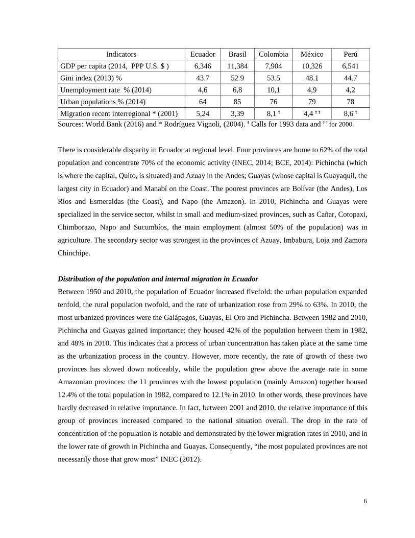
Table 1. International comparison of Ecuador’s social and economic indicators

4 The System of Social Indicators of Ecuador (SIISE, 2014) considers that a person is in extreme poverty if they meet two or more of the following conditions: 1. Their dwelling has inadequate physical characteristics; 2. Their dwelling has inadequate sanitary systems; 3. The household has high economic dependence; 4. There is a child (or children) in the household who does not go to school; 5. The dwelling is in a critical state of overcrowding. 5 The poorest tenth of the population received 1.86% and 1.85% of the national income between 1988 and 2012, whilst the richest tenth received 34.1% and 33.7% in the same period.

6

Indicators Ecuador Brasil Colombia México Perú GDP per capita (2014, PPP U.S. $ ) 6,346 11,384 7,904 10,326 6,541 Gini index (2013) % 43.7 52.9 53.5 48.1 44.7 Unemployment rate % (2014) 4,6 6,8 10,1 4,9 4,2 Urban populations % (2014) 64 85 76 79 78 Migration recent interregional * (2001) 5,24 3,39 8,1 Ϯ 4,4 Ϯ Ϯ 8,6 Ϯ

Sources: World Bank (2016) and * Rodríguez Vignoli, (2004). Ϯ Calls for 1993 data and Ϯ Ϯ for 2000.

There is considerable disparity in Ecuador at regional level. Four provinces are home to 62% of the total

population and concentrate 70% of the economic activity (INEC, 2014; BCE, 2014): Pichincha (which

is where the capital, Quito, is situated) and Azuay in the Andes; Guayas (whose capital is Guayaquil, the

largest city in Ecuador) and Manabí on the Coast. The poorest provinces are Bolívar (the Andes), Los

Ríos and Esmeraldas (the Coast), and Napo (the Amazon). In 2010, Pichincha and Guayas were

specialized in the service sector, whilst in small and medium-sized provinces, such as Cañar, Cotopaxi,

Chimborazo, Napo and Sucumbíos, the main employment (almost 50% of the population) was in

agriculture. The secondary sector was strongest in the provinces of Azuay, Imbabura, Loja and Zamora

Chinchipe.

Distribution of the population and internal migration in Ecuador

Between 1950 and 2010, the population of Ecuador increased fivefold: the urban population expanded

tenfold, the rural population twofold, and the rate of urbanization rose from 29% to 63%. In 2010, the

most urbanized provinces were the Galápagos, Guayas, El Oro and Pichincha. Between 1982 and 2010,

Pichincha and Guayas gained importance: they housed 42% of the population between them in 1982,

and 48% in 2010. This indicates that a process of urban concentration has taken place at the same time

as the urbanization process in the country. However, more recently, the rate of growth of these two

provinces has slowed down noticeably, while the population grew above the average rate in some

Amazonian provinces: the 11 provinces with the lowest population (mainly Amazon) together housed

12.4% of the total population in 1982, compared to 12.1% in 2010. In other words, these provinces have

hardly decreased in relative importance. In fact, between 2001 and 2010, the relative importance of this

group of provinces increased compared to the national situation overall. The drop in the rate of

concentration of the population is notable and demonstrated by the lower migration rates in 2010, and in

the lower rate of growth in Pichincha and Guayas. Consequently, “the most populated provinces are not

necessarily those that grow most” INEC (2012).

7

The changes in the relative importance of each province can be explained partly by transformations in

the country’s production structure. A major downturn in the manufacture and exportation of Panama hats

in the 1950’s led to migration towards the rural areas of the Coast, the Amazon, and abroad (Espinoza

and Achiag, 1981). In the 1960’s there was another major migration process, due to changes in the

agricultural export model (Pachano, 1988). The oil boom (the first oilfield was found in 1962) and the

“process of colonization” 6 made the Amazon a new destination for migration (Guerrero and Sosa, 1996).

In the 1980’s Ecuador was affected by fluctuations in oil production and exportation, natural disasters

and the military conflict with Peru. In 1999, the Ecuadorian economy suffered a serious economic and

financial crisis that had severe effects on unemployment and poverty. It led to high emigration to other

countries, particularly Spain (Bertoli et al., 2011). In 2000, Ecuador introduced dollarization, and a

period of economic stability began. Internal migration between provinces tended to drop, and many

emigrants began to return, due to the international recession and backed by government policy.

Against this background, we analysed changes in interprovincial migration in Ecuador, using census data

from 1982 onwards. Censuses can be used to calculate migration rates by comparing the province of

residence with the province of birth (permanent migration or stock), and with the province of residence

five years before each census (recent migration or flow). Whilst the migrant stock has gradually

increased, from 18.5% in 1982 to 20% in 2010, the flow (recent migrants) has fallen from 8.3% in 1982

to 4.7% in 2010. Therefore, there is a decreasing trend in internal migration flows. Consequently we do

not analyse international migration flows.

The same decreasing trend can be found in Latin America (CEPAL, 2007) for various reasons, according

to Rodríguez Vignoli (2004): the replacement of internal migration by international migration; the

increase in daily journeys for work or study, which eliminate the need to migrate; the increase in home

ownership associated with rising incomes; and a slow-down in migration flows from the countryside to

the city due to the expansion of urbanization. Rodríguez Vignoli does not consider that this is due to a

process of regional convergence. According to CEPAL (2012), in Ecuador migration between areas

6 Since the twenty-first century, measures have been in place to promote the colonization of these areas of the country. In 1885, the “Eastern Province Act” was brought into force, to encourage settlement in the East and to control borders, as Peru was expanding due to rubber activity, which was booming at that time. Among other matters, this Act approved the granting of financial incentives and the free allocation of plots of land to people who moved to the East, as well as various financial benefits for growers of rubber, Chincona, coffee and cacao (Esvertit, 2005). At the start of the 1960s, an agreement was reached to recolonize and resettle the East, to stimulate the impoverished agricultural sector. At the end of 1959, the government obtained funding from international organizations to support this project. In 1964, the Agricultural and Settlement Act was approved, and the Ecuadorian Institute of Agrarian Reform and Settlement (Instituto Ecuatoriano de Reforma Agraria, IERAC) was created to implement the new legislation. The programme involved actions on state properties, followed by semi-public and private properties for social purposes, and finally private properties, and generally followed the FAO’s recommendations (González, 1983).

8

continues and is associated with the multipolar economic development of the country, and the persistence

of chronic poverty in some provinces, which push the population mainly to dynamic provinces or those

with greater opportunities and resources.

Appendix 1 shows the percentage of net migration and the proportion of the total population in each

province. Between 1982 and 2010, except in Pichincha (where the metropolitan area of the capital, Quito,

is situated), all of the Andean provinces were affected by out-migration. Nevertheless, from the 2001

census onwards, this trend was reversed in some Andean provinces, which became net recipients of

migration. In the Coast region, the provinces of Guayas and El Oro, which had been net recipients of

migration, became less attractive to migrants, while the rest of the provinces in the Coast region have net

emigration. The eastern provinces (in the Amazon region) have become less attractive to migrants

overall. As a result, from 2001 most Amazonian provinces were affected by out-migration, although two

of them (Pastaza and Orellana) remained attractive to migrants (expansion of the demographic border

and mining, CEPAL, 2012). In the four censuses that were analysed, the Galápagos attracted migrants,

despite the urban development regulations and the laws on residence in the archipelago, which are

designed to protect the ecosystems and biodiversity. In fact, since 1990 approximately two-thirds of the

resident population in the Galápagos was born outside the province.

3. The gravity model of internal migration in Ecuador, 1982-2010

Theoretical framework and empirical specification

According to models designed by Lewis (1954), Todaro (1969, 1980) and Harris and Todaro (1983),

migrants move from rural or undeveloped areas, with high unemployment and underemployment rates,

poor working conditions and low salaries, to developed, urban areas, with higher levels and/or rates of

productivity growth, as well as better education opportunities, health care and quality of life in general

(Royuela et al., 2010). Any place can be considered a centre of production and consumption, although

urban centres are at an advantage, as they benefit from positive externalities (agglomeration economies),

although excessive concentrations could lead to problems of congestion and social inequalities

(Henderson, 2003). The neoclassical theory of migration is based on the concept of utility maximization:

after a cost-benefit analysis, each individual decides whether or not to migrate, and to which destination

(Borjas, 1988 and 1999). The literature also assumes that migration is selective and depends on

individual characteristics, including sex, age and level of education.

From an aggregate perspective, and taking the work of Ravenstein (1885) as a starting point, migration

models have drawn heavily on gravity models. The economics literature has developed models that result

9

in gravity specifications. Our study is based on a theoretical development given in Beine et al. (2015)7.

Thus, migration from the region of origin 𝑗𝑗 to the region of destination 𝑘𝑘 in the period 𝑡𝑡 (𝑚𝑚𝑗𝑗𝑗𝑗𝑗𝑗) is a

function of the proportion of people who migrate (𝑝𝑝𝑗𝑗𝑗𝑗𝑗𝑗) and the stock of population living in 𝑗𝑗 (𝑠𝑠𝑗𝑗𝑗𝑗).

𝑚𝑚𝑗𝑗𝑗𝑗𝑗𝑗 = 𝑝𝑝𝑗𝑗𝑗𝑗𝑗𝑗𝑠𝑠𝑗𝑗𝑗𝑗 (1)

This is the starting point for the RUM model, which assumes that the utility 𝑈𝑈𝑖𝑖𝑗𝑗𝑗𝑗𝑗𝑗 of an individual 𝑖𝑖

moving from 𝑗𝑗 to 𝑘𝑘 at a time 𝑡𝑡 depends on 𝑤𝑤𝑗𝑗𝑗𝑗𝑗𝑗, the deterministic utility gained by individual 𝑖𝑖 due to

moving from 𝑗𝑗 to 𝑘𝑘 in 𝑡𝑡; 𝑐𝑐𝑗𝑗𝑗𝑗𝑗𝑗, the costs of moving from 𝑗𝑗 to 𝑘𝑘 in time 𝑡𝑡; and ∈𝑖𝑖𝑗𝑗𝑗𝑗𝑗𝑗, an individual stochastic

component of utility:

𝑈𝑈𝑖𝑖𝑗𝑗𝑗𝑗𝑗𝑗 = 𝑤𝑤𝑗𝑗𝑗𝑗𝑗𝑗 − 𝑐𝑐𝑗𝑗𝑗𝑗𝑗𝑗 + ∈𝑖𝑖𝑗𝑗𝑗𝑗𝑗𝑗 (2)

The assumptions about the distribution of the stochastic term in Equation (2) determine the expected

probability of selecting destination 𝑘𝑘. If it is assumed that ∈𝑖𝑖𝑗𝑗𝑗𝑗𝑗𝑗 is stochastic, independent and identically

distributed, according to extreme value type 1, and that the deterministic component of utility does not

vary with the origin 𝑗𝑗 (the expected average utility of not migrating is normalized to zero), then the

expected gross migration flows from 𝑗𝑗 to 𝑘𝑘 could be close to gravity equation (3):

𝐸𝐸�𝑚𝑚𝑗𝑗𝑗𝑗𝑗𝑗� = 𝜙𝜙𝑗𝑗𝑗𝑗𝑗𝑗𝛾𝛾𝑘𝑘𝑘𝑘𝛺𝛺𝑗𝑗𝑘𝑘

𝑠𝑠𝑗𝑗𝑗𝑗 (3)

Where: 𝛾𝛾𝑗𝑗𝑗𝑗 = 𝑒𝑒𝑤𝑤𝑗𝑗𝑗𝑗 ,𝜙𝜙𝑗𝑗𝑗𝑗𝑗𝑗 = 𝑒𝑒−𝑐𝑐𝑗𝑗𝑗𝑗𝑗𝑗 y 𝛺𝛺𝑗𝑗𝑗𝑗 = ∑ 𝜙𝜙𝑗𝑗𝑗𝑗𝑗𝑗 𝜙𝜙𝑗𝑗𝑗𝑗𝑗𝑗 𝛾𝛾𝑗𝑗𝑗𝑗𝑗𝑗∈𝐷𝐷 .

According to Equation (3), expected migration flows depend multiplicatively on (i) 𝑠𝑠𝑗𝑗𝑗𝑗, which is the

capacity of expulsion from 𝑗𝑗 in t; (ii) 𝛾𝛾𝑗𝑗𝑗𝑗 , the capacity of attraction of the destination region 𝑘𝑘; and (iii)

𝜙𝜙𝑗𝑗𝑗𝑗𝑗𝑗< 1, the accessibility of the destination region 𝑘𝑘 to potential migrants from 𝑗𝑗. Expected migration

flows are inversely related to (iv) 𝛺𝛺𝑗𝑗𝑗𝑗, which represents the expected utility of potential migrants from

the situation of origin. The value of this last element increases when accessibility rises (𝜕𝜕𝛺𝛺𝑗𝑗𝑗𝑗 𝜕𝜕𝜙𝜙𝑗𝑗𝑗𝑗𝑗𝑗⁄ >

7 Even this work is devoted to the analysis of international migration, the basic theoretical framework can be applied to any spatial dimension, as any of the assumptions is specific to international frameworks. The RUM model has been extensively used for interregional migration analysis in the literature (e.g. Arzaghi and Rupasingha, 2013). Thus, any difference will be found in the empirical model to be estimated.

10

0), which means that enhanced accessibility of an alternative destination l will invariably lead to a drop

in the expected bilateral flow of migration from 𝑗𝑗 to 𝑘𝑘.

The property of independence of irrelevant alternatives (IIA), which is derived from a distribution

according to McFadden (1974) of the stochastic component of utility in (2), implies that a variation in

the attractiveness or accessibility of an alternative destination (l) leads to a proportional, identical change

in 𝐸𝐸(𝑚𝑚𝑗𝑗𝑗𝑗𝑗𝑗) and 𝐸𝐸(𝑚𝑚𝑗𝑗𝑗𝑗𝑗𝑗). To move from terms of mathematical expectation to an expression based on

data, we must add to Equation (3) a component of the error term 𝜂𝜂𝑗𝑗𝑗𝑗𝑗𝑗, with 𝐸𝐸�𝜂𝜂𝑗𝑗𝑗𝑗𝑗𝑗� = 1, to obtain the

classic gravity model in the literature on migration:

𝑚𝑚𝑗𝑗𝑗𝑗𝑗𝑗 = 𝜙𝜙𝑗𝑗𝑗𝑗𝑗𝑗𝛾𝛾𝑘𝑘𝑘𝑘Ω𝑗𝑗𝑘𝑘

𝑠𝑠𝑗𝑗𝑗𝑗𝜂𝜂𝑗𝑗𝑗𝑗𝑗𝑗 (4)

The IIA axiom may not be true for various reasons, which lead to that known as multilateral resistance

to migration. According to Bertoli et al. (2011), the scale of migration flows between two destinations

depends not only on their relative attractiveness, but also on the attractiveness of alternative destinations.

Therefore, an increase in the attractiveness of a third destination will decrease the probability of

migration flows between the two initial destinations. If this concept is overlooked, biased estimates could

be produced (Bertoli et al., 2013b). Multilateral resistance to migration may arise when assumptions

about the distribution of the stochastic component are altered, or if we consider the sequential nature of

migration decisions.

Population groups in the place of origin may be heterogeneous, and as a result the same destination may

have a different level of attractiveness for them, for example, due to sex, age, level of education or aspects

associated with the psychological costs for different population groups. The existence of this

heterogeneity introduces a pattern of correlation with all destinations into the stochastic component of

utility. According to Bertoli et al. (2013a), if a correlation is assumed to exist in the stochastic component

of utility, then an increase in the attractiveness of a third destination that is perceived as a substitute for

k will reduce the volume of migrants between j and k (𝑚𝑚𝑗𝑗𝑗𝑗𝑗𝑗) proportionally more than the volume of

individuals who decide to remain in the place of origin (𝑚𝑚𝑗𝑗𝑗𝑗𝑗𝑗).

Similarly, we can assume that the model should include not only the present characteristics of the

alternative destinations, but also the future expectations of each one of them (in t+1). Even if we assume

that the stochastic component of utility is independent and identically distributed (IID) and of extreme

11

value type 1, the final model will be sensitive to expectations about the future attractiveness of alternative

destinations (Bertoli at al., 2013b, Beine and Coulombe, 2014). Therefore, in accordance with Hanson

(2010) and Beine et al. (2015), traditional models explain migration flows as a result of different

characteristics in the place of origin and destination, assuming the IIA property and therefore avoiding

multilateral resistance to migration. However, the impact of conditions in the place of origin tends to be

overestimated if the influence of alternative destinations is not considered.

These effects have been controlled in various ways in the literature. When the panel is large enough in

terms of cross-sectional and longitudinal data, the multilateral resistance term adapts to the structure of

the common correlated effects estimator (CCE, Pesaran, 2006) as used, for example, in Bertoli et al.

(2013b) and Bertoli and Fernández-Huertas Moraga (2013). Our case study does not have the right

characteristics to apply this type of techniques. Consequently, we follow the applied migration literature

(see below) and we aim to capture these aspects by using various dummy variable structures, as we have

three data dimensions (origin, 𝑗𝑗, destination 𝑘𝑘, and moment in time 𝑡𝑡).8 Therefore, in this study, we

estimate models with different fixed effects structures, from the simplest model which is a priori biased,

to more complex structures that lose part of the information, but enable us to estimate parameters that

are free of some biases.

1. Basic model with origin and destination variables and time fixed effects.

𝑙𝑙𝑙𝑙 𝑚𝑚𝑗𝑗𝑗𝑗𝑗𝑗 = 𝛼𝛼 + 𝐷𝐷𝑗𝑗 + 𝛽𝛽1𝑋𝑋𝑗𝑗𝑗𝑗𝑗𝑗 + 𝑒𝑒𝑗𝑗𝑗𝑗𝑗𝑗 (5)

Where: 𝛼𝛼 is the intercept, 𝐷𝐷𝑗𝑗 is the vector of dichotomous variables for each year, and 𝑋𝑋𝑗𝑗𝑗𝑗𝑗𝑗 is the vector

of independent variables in the model. The vector of dummy variables for each year enables us to control

common disturbances in time in all provinces. However, if multilateral resistance to migration exists,

this model will produce biased estimates. The inclusion of time fixed effects enables us to capture general

time shocks in all observations. In turn, this enables us to capture the multilateral resistance to migration

of potential destinations that are not included in the database.

2. Panel model with monadic fixed effects of the origin and the destination, and time fixed effects.

𝑙𝑙𝑙𝑙 𝑚𝑚𝑗𝑗𝑗𝑗𝑗𝑗 = 𝐷𝐷𝑗𝑗 + 𝐷𝐷𝑗𝑗 + 𝐷𝐷𝑗𝑗 + 𝛽𝛽1𝑋𝑋𝑗𝑗𝑗𝑗𝑗𝑗 + 𝑒𝑒𝑗𝑗𝑗𝑗𝑗𝑗 (6)

8 See Beine et al. (2011), McKenzie et al. (2013) and Ortega and Peri (2013) for different justifications for the inclusion of these dummies.

12

Where 𝐷𝐷𝑗𝑗 and 𝐷𝐷𝑗𝑗 correspond to dichotomous variables for each origin and destination province

respectively, 𝑋𝑋𝑗𝑗𝑗𝑗𝑗𝑗 is the vector of independent variables in the model, and 𝐷𝐷𝑗𝑗 is again the vector of time

fixed effects. Mayda (2010) includes fixed effects of the origin and destination, to control for specific

effects of each origin / destination that are not captured by deterministic components of utility. This is

the traditional strategy for capturing multilateral resistance to migration in cross-sectional studies. Mayda

(2010) uses it to control for the effect of migration policy that is common to all spatial units. In our case,

it would enable us to capture the permanent migration policy for the Amazonian provinces or the legal

restrictions to immigration in the Galápagos. Nevertheless, this model does not account for most types

of multilateral resistance described above.

3. Panel model with dyadic fixed effects of origin-destination.

𝑙𝑙𝑙𝑙 𝑚𝑚𝑗𝑗𝑗𝑗𝑗𝑗 = 𝐷𝐷𝑗𝑗𝑗𝑗 + 𝐷𝐷𝑗𝑗 + 𝛽𝛽1𝑋𝑋𝑗𝑗𝑗𝑗𝑗𝑗 + 𝑒𝑒𝑗𝑗𝑗𝑗𝑗𝑗 (7)

Where: 𝐷𝐷𝑗𝑗𝑗𝑗 is the vector of dichotomous variables of origin-destination. This specification is similar in

nature to the above, with the added feature that we can now quantify specific deterministic effects for

each pair of regions (Ortega and Peri, 2013). This fixed effects structure captures any specific bilateral

relationship between j and k, which reflect fixed migration costs, geographic aspects and historic

migration networks between pairs of regions, and even permanent migration policies. This structure also

includes constant specific characteristics of the origin and destination. However, the distance variable is

not included in this model: to the extent that it remains constant for each pair of regions (Karemera et

al., 2000; Ortega and Peri, 2013), it shows perfect multicollinearity with this fixed effects structure.

4. Panel model using origin variables of origin and dyadic fixed effects of destination-time.

𝑙𝑙𝑙𝑙 𝑚𝑚𝑗𝑗𝑗𝑗𝑗𝑗 = 𝛼𝛼 + 𝐷𝐷𝑗𝑗𝑗𝑗 + 𝐷𝐷𝑗𝑗 + 𝛽𝛽1𝑋𝑋𝑗𝑗𝑗𝑗 + 𝑒𝑒𝑗𝑗𝑗𝑗𝑗𝑗 (8)

Where: 𝐷𝐷𝑗𝑗𝑗𝑗 is the vector of the destination’s dyadic dummy variables for each year, while 𝑋𝑋𝑗𝑗𝑗𝑗 is the

vector of independent variables of the origin regions. This panel model enables us to control for all of

the “pull” determinants of migration, and particularly multilateral resistance derived from heterogeneity

in the future perspectives of the destination regions (Beine and Parsons, 2012). The structure also enables

us to control for time-invariant characteristics of migration policies that are the same for all provinces.

Beine and Parsons (2012) used dyadic fixed effects of destination-time to control for any specificity

between potential destinations for any period of time. This method can be used to control for bias in the

parameters of the origin variables due to multilateral resistance caused by the heterogeneity of

expectations about each destination. Like Beine and Parsons (2012), we also include fixed effects for

13

each origin. To be clear, this will be our preferred model to capture the parameters associated to the

characteristics of the origin.

5. Ordinary least squares with destination variables and dyadic fixed effects of origin-time

𝑙𝑙𝑙𝑙 𝑚𝑚𝑗𝑗𝑗𝑗𝑗𝑗 = 𝛼𝛼 + 𝐷𝐷𝑗𝑗𝑗𝑗 + 𝐷𝐷𝑗𝑗 + 𝛽𝛽1𝑋𝑋𝑗𝑗𝑗𝑗 + 𝑒𝑒𝑗𝑗𝑗𝑗𝑗𝑗 (9)

Where: 𝐷𝐷𝑗𝑗𝑗𝑗 is the vector of the origin’s dichotomous variables for each year. This method enables us to

control for all the “push” determinants of migration, as well as the multilateral resistance derived from

heterogeneity in migration preferences by origin. Ortega and Peri (2013) use these dyadic fixed effects

of origin-time to control for any specificity in the place of origin in any period of time. This approach

can be used to eliminate the bias in the parameters of the destination associated with multilateral

resistance due to heterogeneity in preferences of migration by origin. Bertoli and Fernández-Huertas

Moraga (2012) use a cross-section model to estimate heterogeneity in preferences by destination

subgroups, with dummy variables to control for these subgroups, which we do not consider in this study.

To be clear, this will be our preferred model to capture the parameters associated to the characteristics

of the destination.

Given the nature of the proposed panel of models, a structure of the random term that is only associated

with idiosyncratic errors 𝑒𝑒𝑗𝑗𝑗𝑗𝑗𝑗 could be assumed for the estimation. Alternatively, we could also assume

the existence of a structure composed of permanent individual errors, corresponding to the fixed structure

of the panel, that is, for each pair of regions [𝜉𝜉𝑗𝑗𝑗𝑗]. The second case represents a random effects model,

which increases the efficiency of the estimation. Given that in most cases the fixed effects structures will

control for unwanted consequences of random effects models, we will generally use the panel estimation

assuming the existence of specific random effects for each pair of regions.

One issue not covered in the theoretical approach of the model presented here is the selection of

deterministic factors for the function of the utility of individuals. In the empirical literature, the most

common aspects are pull factors and opportunities to earn an income at the destination (Mayda, 2010),

the gap in income per capita between the origin and the destination (Ortega and Peri, 2009), the

population in the place of origin and the income at the destinations (Karemera et al., 2000), the

differences in terms of quality of life (Faggian and Royuela, 2010) or the level of urbanization (Royuela,

2015). Given the assumption of normalization in the utility at origin, the deterministic component of

utility in the empirical model measures the effect of increasing the gap in expected benefits between the

origin and the destination. According to empirical literature on migration, we can apply the relative

14

difference in the deterministic component of utility to the variable that approximates material welfare

(Beine and Parsons, 2012, use the log of the income ratio, while Ortega and Peri, 2009, analyse both

linear and logarithmic differentials).

Attractiveness is estimated using the distance between the origin and the destination, which can be

determined physically (using the Euclidean distance or distance by road) or economically (the average

distance in terms of time), or it can be derived from differences in terms of language, customs, history,

culture, and institutions (Belot and Ederveen, 2012; Caragliu et al., 2012).

Very few studies on this research area relate to Ecuador. Studies that do refer to this country mainly

focus on the influence of international migration. Notable studies are those by Gratton (2007) on the

characteristics of migration from Ecuador to Spain and the United States; Bertoli et al. (2011 and 2013a),

who analysed how migration policy redirected traditional migration to the United States to Spain; a study

on the relation between migration, remittances and environmental variables in rural communities of

Ecuador by Gray (2009 and 2010); and, finally, an analysis of how migration affects family structure

and fertility (Laurian et al., 1998).

The empirical model for Ecuador

The proposed empirical model analyses the flow of recent migrations by province of origin and

destination, using databases of Ecuador’s Census of Population and Housing (CPV) from 1982, 1990,

2001 and 2010. Today, Ecuador has 24 provinces. The provinces of Sucumbíos and Orellana were

created in 1989 and 1998 respectively, when they were separated from Napo province. Santo Domingo

de los Tsachillas and Santa Elena, which had belonged to the provinces of Pichincha and Guayas

respectively, became provinces in 2007. To work with a standardized database for the entire period, we

added data from the province of Orellana to that of Napo, Santa Elena to Pichincha, and Santo Domingo

to Guayas, to obtain a total of 21 provinces. We did not take into account non-delimited areas, as these

are not representative at national level.9 Recent internal migration refers to the population that changed

residence in the five years prior to the census. Consequently, it does not include migration that occurred

at an earlier time. To avoid problems of simultaneity, the explanatory variables in the model refer to the

previous census, so that migration flows between 2005 and 2010 are explained by the characteristics of

the provinces in 2001. As the dependent and the explanatory variables are separated five years, we

9 We did not consider migration data for Sucumbíos for 1982, as this information was added to that of the province of Napo. In Ecuador, 1,419 km² of the territory is not assigned to any province. In 2010, these territories had 32,384 inhabitants and corresponded to the areas of Las Golondrinas, La Manga del Cura and El Piedrero.

15

minimize the chance that a shock could be affecting simultaneously both the dependent and the

explanatory variables. As in Rupasingha et al. (2015) and Levine et al. (2000), we understand that future

migration does not affect current levels of explanatory variables. We also used information from the

1974 census to calculate control variables for the characteristics of the origin and destination of migration

flows for the 1982 census. Finally, as Beine et al. (2015) argue, “controlling for multilateral resistance

to migration can make instrumentation unnecessary as long as the endogeneity problem is not due to

reverse causality, or as long as the resistance terms capture a big part of the omitted factors” (p.9).

As explanatory variables, we included basic gravity factors: the population of origin and destination and

the distance between them, which approximates the costs associated with migration (Peeters, 2012). The

distance variable can be measured in kilometres and expressed in logarithms (L Dist), as in Mayda

(2010), or in terms of time (L Time), which is closer to the economic concept of the cost of moving10.

We used proportions of employment by branches of activity to control for the sector structure. In general,

greater importance of the agricultural sector is traditionally associated with a lower level of development.

The most developed provinces were expected to have a higher proportion of people employed in

manufacture (Manufacturing_Ind) and services (Services) and less employment in primary activities,

including agriculture (Agriculture) and mining and quarrying (Mines & Quarrying). The construction

sector was also included in the analysis (Construction). We also considered the characteristics of the

labour market (LM) according to whether workers received salaries (LM-Employee); were owners or

partners (LM-Partner), or were involved in another form of employment (LM-Other).

The probability of obtaining higher income levels is a key factor in the decision to migrate. To represent

this, Karemera et al. (2000) used gross value added (GVA), Mayda (2010) used the average salary of

employees, while Ortega and Peri (2009) and Beine and Parsons (2012) considered GDP per capita. The

Ecuadorian census does not include salary information, and gross value added data was not available for

provinces for the entire study period. Therefore, in order to take into account the concept of different

material characteristics in the place of origin and the destination, we used census information on the

condition of dwellings, including their structural characteristics, the water supply, the existence of a

sewer system and access to electricity. We constructed an index of material conditions (Relative Index

Material WB) for provinces up to 1974 by regressing the non-oil GDP per capita on indicators of the

10 The variables of physical distance and time were obtained from two sources: Ecuador’s yellow pages (L Dist Y-P) and Google Maps (L Dist Google). We added the Euclidean distance between the capitals in each of the provinces (L Dist Crow). The distances for the Galápagos Islands were calculated by adding the distance to the closest province with an air link (Pichincha and Guayas).

16

conditions of dwellings, and keeping the estimated coefficients constant.11 Again, we lagged such

indicator five years before the initial period of the dependent variable, there is a chance that migrants

anticipate future changes of income. Models 4 and 5, including destination-time and origin-time fixed

effects respectively, remove bias due to omitted variables in the destination (model 4) and origin (model

5) region. In addition, our measurement of material welfare, based on housing characteristics, is much

less cyclical than any wages or income variable. We have no information for amenities in our data set.

Nevertheless, the variable that we use for capturing material conditions of people is both just a proxy of

income and at the same time an indicator of the material living conditions of the population. Given the

structure of fixed effects in the empirical models, we account for permanent natural and human made

amenities in both origin and destination.

As an additional approximation to control for the level of income and the selectivity of migrants, we

used the level of education (No Education, Primary, Secondary and Higher Education). A higher level

of education is expected to enable a higher salary to be obtained. Likewise, higher levels of education in

the place of origin are expected to be associated with a higher level of migration. Similarly, given that a

population’s characteristics determine the propensity to migrate, we considered age cohorts in the

regression analyses.

We considered the rate of urbanization (Urbanization rate) as a pull factor for migration. Urbanisation

is associated with economic and social development: increasing industrial expansion, higher productivity

and salaries, greater probability of finding work and a better quality of life, despite the high level of

urban unemployment. Since Alfred Marshall (1890) there is a theoretical framework proving

agglomeration economies. The causes of agglomeration economies are addressed by Duranton and Puga

(2004), Rosenthal and Strange (2004) and Puga (2010) among many others. Various studies relate

empirical findings of a growth augmenting result of various measures of urbanisation (including urban

concentration) on countries’ income in the long run (such as Henderson, 2003; Brülhart and Sbergami,

2009).

11 In addition to the regression model, we considered other alternatives based on information about dwelling indicators (arithmetic means and principal components). Details of the construction of the index that was finally used and the alternative indices can be found in the Additional Material.

17

Table 2. Statistical description of variables Migration jk Average St.Dev. Min. Q1 Q2 Q3 Max. Asymmetry

1982 1466 4981 0 50 181 752 72843 9.29 1990 1235 3050 1 85 225 847 34123 5.43 2001 1306 3452 1 77 239 858 39511 6.14 2010 1369 3004 4 107 335 973 23388 4.06

Standar deviation Correlation

with L Migration

Correlation with L Pobl Media Overall Between Within Min Max

L Migration k 5.31 1.68 1.63 0.39 0 9.54 1 L Pop k 12.42 1.27 1.23 0.31 8.3 15.19 0.518 1 L Dist-crow jk 5.40 0.80 0.80 0 3.12 7.2 -0.565 -0.089 L Dist-Google jk 5.92 0.69 0.69 0 3.48 7.39 -0.580 -0.112 L Time-Google jk 5.75 0.54 0.54 0 3.71 6.69 -0.498 -0.095 L Dist-YP jk 5.94 0.69 0.69 0 3.71 7.39 -0.585 -0.122 L Time-YP jk 5.56 0.61 0.61 0 3.4 6.58 -0.512 -0.128 Urbanization rate (%) k 41.9 18.66 16.62 8.25 6.85 20.71 0.408 0.309 Agriculture (%)k 44.21 16.7 14.37 8.3 9.06 76.85 -0.383 -0.314 Mines & Quarrying (%)k 0.91 1.74 1.51 1.02 0 12.63 -0.271 -0.200 Manufacturing Ind (%)k 9.02 5.62 5.29 1.89 2.95 27.28 0.248 0.393 Industry Other (%)k 0.39 0.23 0.14 0.18 0.04 1.11 0.270 0.322 Construction (%)k 5.41 2.04 1.36 1.51 1.19 11.46 0.224 0.140 Services (%)k 40.07 13.72 11.51 7.32 16.64 75.03 0.375 0.220 LM-Partner (%)k 49.17 9.62 4.67 8.42 22.92 69.65 -0.018 0.195 LM-Employee (%)k 39.87 11.03 7.11 8.42 18.61 69.13 0.177 -0.031 LM-Other (%) k 12.13 5.06 3.92 3.17 1.17 31.11 -0.332 -0.302 No Education (%)k 16.01 9.98 5.61 8.29 2.21 45.15 -0.136 -0.078 Primary Education (%)k 52.00 10.16 4.53 9.07 27.53 69.94 -0.269 -0.245 Secondary Education (%)k 25.45 12.81 5.11 11.78 5.21 48.92 0.165 0.142

Higher Education (%)k 6.45 4.96 2.77 4.1 0.35 22.34 0.389 0.294 Pop_0_4 (%)k 14.09 2.53 1.53 2 10.03 19.79 -0.332 -0.428 Pop _5_9 (%)k 13.38 1.9 1.09 1.55 9.56 17.3 -0.337 -0.325 Pop _10_14 (%)k 12.42 1.24 0.8 0.94 8.68 14.81 -0.276 -0.076 Pop _15_19 (%)k 10.44 0.74 0.48 0.56 8.21 12.3 -0.190 0.098 Pop _20_24 (%) k 8.87 0.97 0.8 0.55 7.13 11.8 0.253 0.002 Pop _25_29 (%)k 7.44 1.14 1 0.52 5.81 11.99 0.218 -0.157 Pop _30_34 (%)k 6.33 0.93 0.73 0.58 4.79 9.83 0.260 0.005 Pop _35_39 (%)k 5.54 0.75 0.44 0.62 4.29 8.68 0.241 0.134 Pop _40_49 (%)k 8.59 1.31 0.62 1.15 6.31 13.4 0.259 0.306 Pop _50_59 (%)k 5.84 1.18 0.74 0.93 3.55 8.23 0.235 0.391 Pop _60_69 (%)k 3.93 1.13 0.87 0.71 1.78 6.47 0.154 0.361 Pop _70+ (%) k 3.39 1.44 1.08 0.96 1.09 6.59 0.136 0.382 Index Material WB (%) k 6224.9 2141 1709 1292 2519 12544 0.355 0.411

If urbanisation is expected to promote economic growth, it is likely to be associated with higher

opportunities and larger migration flows. In addition, as underlined by Rodríguez-Pose and Ketterer

(2012), “economic and noneconomic territorial features have been found to be essential elements

determining utility differentials, and hence migration incentives of potential movers, across different

territories” (p. 536). A significant number of man-made amenities are efficiently produced in urban areas.

Thus, cities lead to more opportunities, and consequently spread the “capabilities” a-la-Sen (Sen, 1987),

and improve the well-being of individuals. By the same arguments, we would expect a high rate of

urbanization in the place of origin to act as a brake on emigration.

18

Both the dependent variable and the explanatory variables are expressed in logarithms, with the

exception of variables that were already expressed as percentages. Consequently, the coefficients are

interpreted as elasticities. Table 2 shows the descriptive statistics of the variables considered in the

model.

6. Estimation and results

Basic results

In this section, we present the results of estimating the models described in Section 3, using a panel data

analysis and considering random effects. A robust estimation of standard errors was made, and we

assumed the presence of a potential time correlation between the observations at origin-destination

(Models 1 to 3), destination (Model 4) and origin (Model 5) level. The estimated models measure the

impact of push and pull variables on migration flows, as well as the characteristics of resident individuals,

to control for the selectivity of migrants to a certain extent. Models 4 and 5 report estimates free of bias

resulting from different types of multilateral resistance and will be our preferred models. Table 4 presents

the results of all models for comparison.

The distance measure considered was the logarithm of the distance between provincial capitals, which

was based on the time it takes to travel on the best route by road, according to Google Maps. In all the

estimated models, the parameter associated with this variable was negative, as expected. When fixed

effects structures were considered the parameter gets bigger, what stressed the importance of space once

local specificities are taken into account.

The index that shows relative differences in material welfare was not significant in Model 4. As this

specification controls for the destination’s specific circumstances, we could state that lower levels of

material welfare in the place of origin do not lead to an increase in migration. On the contrary, in Model

5, controlling for origin specific factors, we observe a positive and significant parameter. The elasticity

is 0.16, a result within the range of results for GDP pc in Caragliu et al. (2013) at the international level,

much higher than Rupasingha et al. (2015) for wages at the county level in the US, and close to some of

the results in Arzhaghi and Rupasingha (2013) for rural urban migration between US counties.

Consequently, we can conclude that material welfare acts as a pull factor for migrants in Ecuador.

Variables related to population structure had significant parameters with different signs, which we

interpret as a control for the selectivity of emigrants in the place of origin. Model 4 reports lower

19

migration from regions with younger (between 20 and 24) and older (above 70) residents, but higher

migration for regions with higher porportions of residents between 25 and 29. It is more difficult to

interpret the results for the destination, as different signs were found for very close age cohorts. However,

the signs and, in most cases, the signficance were maintained in the different specifications of the gravity

model, which indicates that the impact of the age structure on migration is not affected by bias due to

multilateral resistance to migration.

The provinces that had high proportions of the population with primary and secondary levels of education

were those with the highest levels of emigration. In contrast, provinces with increasing proportions of

the population with higher education qualifications did not have differential levels of migration. The

education structure in the destination does not appear to be a pull factor or a barrier to migration flows.

In terms of the structure of employment by sector, we found that a highly cyclical sector such as

construction is always associated with significant parameters for the place of origin and destination. This

confirms empirical evidence in other studies indicating that migration flows are more feasible in periods

of expansion and increasing housing availability than in times of recession. For the destination, the

manufaturing industry sector was a significant parameter in all the models we considered. The fact that

development associated to the growth in manufacturing industry was significant is in favor the Harris-

Todaro models of rural-urban transformation associated to development. On the contrary, the estimates

did not report a significant impact of the weight of mining industries as a pull factor, what contrasts the

role of the oil sector on making the Amazon an atractive destination for migrants.

The strucuture of the labour market only appears to have a degree of influence at the place of origin.

Thus, in Model 4 the “LM-Others” category was associated with a marginally significant, positive

parameter. Therefore, structures that could be related to underempoyment in the place of origin could be

considered push factors.

20

Table 3. Basic results of gravity models 1 to 5.

Model 1 Model 2 Model 3 Model 4 Model 5 L Time Dist Google -1.387*** (0.0741) -1.639*** (0.0746) -1.634*** (0.0889) -1.639*** (0.0983) Relative Index Material WB 0.0382 (0.0336) 0.0651** (0.0286) 0.0733*** (0.0282) -0.00614 (0.0303) 0.163*** (0.0371) L Population_O 0.890*** (0.0367) 0.745*** (0.156) 0.750*** (0.154) 0.721*** (0.0921) Urbanization rate_O -0.0102*** (0.00310) -0.0185*** (0.00359) -0.0185*** (0.00354) -0.0188*** (0.00295) Pop_10_14_O 0.0217 (0.0463) -0.0202 (0.0487) -0.0223 (0.0481) -0.00451 (0.0338) Pop_15_19_O -0.0337 (0.0382) 0.0171 (0.0409) 0.0181 (0.0403) -0.00463 (0.0442) Pop_20_24_O -0.118*** (0.0423) -0.162*** (0.0430) -0.162*** (0.0424) -0.158*** (0.0501) Pop_25_29_O 0.198** (0.0838) 0.163** (0.0790) 0.160** (0.0779) 0.167* (0.0924) Pop_30_34_O -0.0436 (0.0984) 0.0140 (0.0973) 0.0156 (0.0959) 0.0135 (0.104) Pop_35_39_O -0.0260 (0.0838) -0.0204 (0.0841) -0.0240 (0.0830) -0.0114 (0.111) Pop_49_49_O 0.0264 (0.0471) 0.0109 (0.0490) 0.0125 (0.0484) 0.0141 (0.0501) Pop_50_59_O -0.0104 (0.0668) 0.0302 (0.0688) 0.0231 (0.0678) 0.0294 (0.0670) Pop_60_69_O -0.0589 (0.0933) 0.0369 (0.105) 0.0320 (0.104) 0.0494 (0.0851) Pop_70m_O -0.173** (0.0795) -0.249*** (0.0817) -0.246*** (0.0807) -0.257*** (0.0771) Primary Education_O 0.0175*** (0.00585) 0.0105 (0.00650) 0.0105 (0.00641) 0.0107* (0.00590) Seconday Education _O 0.0277*** (0.00973) 0.0226* (0.0119) 0.0226* (0.0118) 0.0238** (0.00985) Higher Education O 0.00380 (0.0133) -0.0103 (0.0159) -0.00986 (0.0157) -0.0138 (0.0150) Mines & Quarrying_O -0.00730 (0.00846) -0.00642 (0.00991) -0.00673 (0.00976) -0.00758 (0.0114) Manufacturing Ind_O 0.00513 (0.00664) 0.0141* (0.00771) 0.0136* (0.00761) 0.0147 (0.00975) Industry Other _O 0.107 (0.0977) 0.0358 (0.102) 0.0272 (0.101) 0.0716 (0.0867) Construction_O 0.0320** (0.0127) 0.0485*** (0.0139) 0.0492*** (0.0137) 0.0388*** (0.0140) Services_O 0.00991 (0.00654) -0.00660 (0.00747) -0.00641 (0.00738) -0.00542 (0.00641) LM-Employee_O -0.00348 (0.00419) 0.00230 (0.00423) 0.00213 (0.00416) 0.00229 (0.00374) LM-Other _O 0.00229 (0.00522) 0.00860 (0.00569) 0.00846 (0.00560) 0.00889* (0.00531) L Population_D 0.579*** (0.0431) -0.695*** (0.156) -0.690*** (0.154) -0.669*** (0.142) Urbanization rate_D -0.00336 (0.00372) 0.00356 (0.00439) 0.00345 (0.00432) 0.00197 (0.00404) Pop_10_14_D -0.0737 (0.0495) 0.0325 (0.0500) 0.0328 (0.0493) 0.0453 (0.0432) Pop_15_19_D 0.172*** (0.0431) 0.107** (0.0447) 0.105** (0.0441) 0.0863* (0.0466) Pop_20_24_D -0.00920 (0.0459) -0.0513 (0.0427) -0.0502 (0.0421) -0.0477 (0.0447) Pop_25_29_D 0.151* (0.0815) -0.0597 (0.0784) -0.0640 (0.0773) -0.0666 (0.0655)

21

Pop_30_34_D -0.0464 (0.0951) 0.176* (0.0952) 0.182* (0.0940) 0.206** (0.0852) Pop_35_39_D -0.280*** (0.0862) -0.151* (0.0880) -0.155* (0.0867) -0.153** (0.0773) Pop_49_49_D 0.195*** (0.0538) 0.245*** (0.0546) 0.247*** (0.0539) 0.238*** (0.0432) Pop_50_59_D -0.229*** (0.0673) -0.254*** (0.0688) -0.259*** (0.0679) -0.235*** (0.0665) Pop_60_69_D -0.130 (0.0864) -0.249** (0.0981) -0.254*** (0.0967) -0.234*** (0.0902) Pop_70m_D -0.0885 (0.0709) 0.135* (0.0742) 0.138* (0.0730) 0.131** (0.0553) Primary Education_D 0.00606 (0.00544) 0.00644 (0.00605) 0.00651 (0.00597) 0.00766 (0.00703) Seconday Education _D -0.0181* (0.00936) 0.00363 (0.0108) 0.00373 (0.0106) 0.00456 (0.0104) Higher Education D 0.00403 (0.0131) 0.00136 (0.0152) 0.00115 (0.0151) -0.00211 (0.0140) Mines & Quarrying_D -0.0431*** (0.0104) -0.0101 (0.0120) -0.0106 (0.0119) -0.0109 (0.0115) Manufacturing Ind_D 0.0174*** (0.00511) 0.0168** (0.00673) 0.0167** (0.00663) 0.0171*** (0.00509) Industry Other_D 0.114 (0.110) 0.0294 (0.111) 0.0293 (0.110) 0.0619 (0.124) Construction_D 0.101*** (0.0146) 0.0649*** (0.0138) 0.0642*** (0.0136) 0.0591*** (0.0110) Services_D 0.0298*** (0.00623) 0.00648 (0.00698) 0.00688 (0.00689) 0.00728 (0.00620) LM-Employee_D -0.0105** (0.00422) -0.00298 (0.00432) -0.00298 (0.00426) -0.00119 (0.00319) LM-Other_D 0.00697 (0.00493) -0.00125 (0.00530) -0.00121 (0.00524) 0.000368 (0.00425) Constant -6.142*** (2.011) 12.68*** (3.396) 2.660 (3.180) 6.024*** (1.921) 21.60*** (2.875)

Fixed effects Time Time, origin and

destination Time and origin -

destination Destination -time and

origin Origin-time and

destination Observ / Nº groups 1,600 420 1,600 420 1,600 420 1,620 420 1,620 420 Overall R2 0.796 0.877 0.979 0.880 0.878 Within / Between R2 0.404 0.796 0.473 0.891 0.473 1.000 0.555 0.890 0.531 0.891

Note: Significance: *:10%; **:5%; ***:1%. Standard errors are given in brackets (robust, and with the possibility of correlation between the various dyadic origin-destination structures). The default categories are Population below 10 years, No Education, Agriculture sector, and LM-Owner Partner.

22

Finally, we paid special attention to the population variable and to the rate of urbanization. Model

4 showed how provinces increasing in size pushed out larger numbers of the population, which

simply confirms a question of scale that is inherent in gravity models. As also expected, greater

and increasing rates of urbanization in the place of origin were factors linked to lower levels of

migration. The models that control for multilateral resistance to migration to a greater or lesser

extent indicated a greater influence of urbanization than observed in Model 1. Model 4, which

controls for the heterogeneity of expectations about the destination, showed a negative impact of

urbanization in the place of origin that was 84% higher than the parameter in Model 1. In other

words, there are fewer reasons to leave provinces with higher rates of urbanization (more and

better services, a priori), and there may be different expectations, perhaps because there is better

information about destinations.

The destination’s level of population and rate of urbanization are variables with parameters that

require deeper reflection. Model 5 reported a significant negative parameter for population, while

the urbanisation rate was not significant. This result could be surprising, but is in line with the

description in Section 2, which indicated a drop in the rate of population concentration in the most

populated provinces, and that “the most populated provinces are not necessarily those that grow

most” (INEC, 2012). In fact, 41% of the urban population was concentrated in the three most

urbanized provinces (Galápagos, Guayas and Pichincha) in 1982. This proportion continued to be

41% in 2010, due to the notable increase in the rate of urbanization in the other provinces.

Model 1 found a positive, significant parameter for population size. In order to understand such

dramatic difference, we follow Baltagi and Griffin (1984) and Pirotte (1999). If we would assume

a dynamic relationship, the fixed-effects estimates would capture the short-run impact of the

variable, being the pool and random effects estimations a mix of the long (which would be

captured by the between estimate) and short estimates. Consequently, Model 1 showed how most

populated provinces are recipients of larger population flows. On the contrary, Model 5 reported

that most growing provinces are not the ones receiving higher migration flows. We interpreted

these results suggesting that the recent process of development in Ecuador is not driving to deepen

territorial concentration, particularly due to the growth of medium-sized and small cities in

comparison to the large metropolises of Guayaquil and Quito.

Analysis of sensitivity and robustness

We then estimated the specifications of the model using different measures and sub-samples. Next

we included the analysis dividing the full sample in two subberiods. Table 4 displays the results

of models 4 and 5 for the subperidos 1982-1990 and 2001-2010. We only present the results of

distance, the material well being index and the ones for population and urbanisation rate. The

23

regressions for the 1982-1990 subperiod, where urbanisation was substantially lower, the

urbanisation rate was relatively more important to retain population. When we considered

variables associated to destination, the process of population concentration was taking place, as

population mattered more as pull factor. On the second subperiod, though, urbanisation is less

important. These results contrast with the ones obtained for the full sample. In any case, it is very

important to take into account that the global model results are not purely an average between

subperiods and consequently that the variance between subperiods matters for understanding

results of the final model. Consequently the results obtained for the full data set are describing a

40 years story, in a contry where urbanisation has boomed and the regional population flows have

decreased.

Table 4. Results by subperiods

Model 4 Model 5 1982-1990 2001-2010 1982-2010 1982-1990 2001-2010 1982-2010 L Time Dist Google -1.694*** -1.582*** -1.634*** -1.706*** -1.582*** -1.639*** Relative Index Material WB -0.310 0.0335 -0.00614 -0.321** 0.0335 0.163*** L Population_O 1.635*** 3.339*** 0.721*** Urbanization rate_O -0.0898*** -0.0110 -0.0188*** L Population_D 2.920*** 1.093 -0.669*** Urbanization rate_D -0.0710*** 0.00361 0.00197

Given that one of the parameters of greatest interest in the study corresponded to the destination’s

population and the rate of urbanization at the destination, we then assessed the robustness of the

results, excluding the destinations of the provinces of Pichincha and Guayas on the one hand, and

the Galápagos on the other. Table 5 shows the estimates of the parameters. It be seen that the

signs and significance of the parameters were similar when these provinces were excluded.

Finally we also tested the influence of the Oil production in the Amazon. Even though we

controlled for the weight of such sector, we removed from the sample the three provinces where

Mining and Quarrying display a stronger role (Napo, which considers Orellana, Sucumbios,

Zamora Chinchipe). The results displayed a non significant parameter for population and a

positive and significant parameter for the urbanization rate. Even though the Oil producer regions

have experienced a huge urbanisation process, they have been attracting decreasing amounts of

migrants. Given their particular characteristics, one they are excluded from the sample we observe

how the overall growth in urbanisation in the country has acted as brake in the process of

population concentration: many rural provinces that in the 70’s had double digit emigration rates

have experienced a a joint course of urbanization and retention of population.

24

Finally, we acknowledge that despite our concerns and the design of our empirical exercise,

endogeneity could be affecting our results if there were shocks affecting both migration and

population simultaneously, biasing the population coefficient and consequently affecting other

parameters. We have performed additional estimates (not reported) removing population as an

explanatory variable. These computations shows very minor absolute changes in the parameters

of the main explanatory variables, and no change is observed in their significance.

Table 5. Sensitivity of parameters associated with the destination’s population and rate of

urbanization Model 1

Total Sample Without

Pichincha and Guayas

Without the Galápagos

Without the Oil Provinces ¥

L Population_D 0.579*** 0.508*** 0.347*** 0.537*** Urbanization rate_D -0.00336 -0.00271 -0.000497 0.00818**

Model 5 L Population_D -0.669*** -0.375** -0.759*** -0.019 Urbanization rate_D 0.00197 0.000610 -0.00568 0.00977**

¥ The provinces spesialized in oil are Napo (which considers Orellana), Sucumbios, Zamora Chinchipe, as both have an average of employment in this sector above 3%.

7. Conclusions

In this study, we analysed determinants of migration flows in Ecuador between 1984 and 2010

by estimating gravity models. To obtain robust parameters with no bias from multilateral

resistance to migration, we estimated a range of specifications using different fixed effects

structures.

The main results obtained are in line with the empirical literature on different countries. Thus,

migration flows were greater between more populated provinces that were close to each other.

The relative index material wellbeing raised as a pull factor, as the estimations showed significant

parameters for the destination regions. The education structure in the destination does not appear

to be a pull factor or a barrier to migration flows, while the sectoral composition of the economy

had a significant role: the Construction sector reported significant parameters both at the origin

and at the destination, while Manufacturing Industry had a key role attracting migrants, in line

with the Harris Todaro transformation models. Labour markets with structures close to under-

employment in the place of origin could be considered push factors.

25

Finally, we paid special attention to the role of population and urbanization. In the descriptive

analysis we found that population flows tend to be towards the most populated provinces, but the

concentration rate has dropped over time. Consequently, in recent periods the largest provinces

have not been those with the most growth. The estimated models confirmed such trend: territorial

concentration has slowed due to the growth of medium-sized and small cities. The sensitivity

analysis allowed us to see that the urbanization process in the whole country was acting as

deterrent factor for population concentration that is favoured. To be clear, we could consider that

a process of territorial balance is occurring in Ecuador, in which growth in provinces, associated

to urbanization, is hampering territorial concentration.

In terms of economic policy, the results highlight the importance of understanding jointly the

migration and urban phenomenon as a factor that shapes the distribution of a population in space.

Consequently, the provision of basic resources (including education and health) should be

increased in parallel, or even proportionally more, in small and medium-sized cities.

Agglomeration economies could be better exploited if, in practice, increasing levels of

urbanization were accompanied by elements that contribute to making better use of the larger size

of cities (Castells-Quintana, 2016).

Additional work is required for further understanding of regional migration flows in Ecuador,

including the role of international migrations in substituting some internal flows, different

behaviours for alternative educational levels, and the inspection of shorter distance flows, such as

the ones that take place at the canton level.

8. References

- Arzaghi, M. and Rupasingha, A. (2013). Migration as a way to diversify: evidence from rural to urban migration in the U.S. Journal of Regional Science, Vol. 53 No. 4, pp. 690-711.

- Baltagi, B. H., and J. M.Griffin. (1984). Short and Long Run Effects in Pooled Models. International Economic Review 25(3):631–45

- Banco Central del Ecuador (BCE) (2014). [online - Date accessed: 18 July 2014]. Available at: http://www.bce.fin.ec/index.php/cambio-de-ano-base.

- Barca, F., McCann, P. and Rodríguez-Pose, A. (2012). The case for regional development intervention: place-based versus place-neutral approaches. Journal of Regional Science, 52(1), 134-152.

- Barro, R. and Sala-i-Martín, X. (1991) Convergence Across States and Regions, Brookings Papers on Economic Activity, 1991(1), 107-182.

- Beine, M., Bertoli, S. and Moraga, J. F. H. (2015). A practitioners' guide to gravity models of international migration. The World Economy, forthcoming.

- Beine, M., F. Docquier, and C. Ozden (2011) ”Diasporas", Journal of Development Economics, 95(1), 30-41.

- Beine, M., and Coulombe, S. (2014). Immigration and Internal Mobility in Canada (No. 4823). CESifo Group Munich.

26

- Beine, M. A. and Parsons, C. R. (2012). Climatic factors as determinants of International Migration.

- Belot, M., and Ederveen, S. (2012). Cultural barriers in migration between OECD countries. Journal of Population Economics, 25(3), 1077-1105.

- Bertoli, S., Fernández-Huertas Moraga, J., andOrtega, F. (2011). Immigration policies and the Ecuadorian exodus. The World Bank Economic Review, 25(1), 57-76.

- Bertoli and Fernández-Huertas Moraga (2012). Visa policies, networks and the cliff at the border. Documentos de trabajo (FEDEA), (12), 1.

- Bertoli, S., Fernández-Huertas Moraga, J. and Ortega, F. (2013). Crossing the border: self-selection, earnings and individual migration decisions. Journal of Development Economics, 101, 75-91.

- Bertoli, S., Brücker, H.and Fernández-Huertas Moraga, J., (2013b) "The European Crisis and Migration to Germany: Expectations and the Diversion of Migration Flows," Working Papers 2013-03, FEDEA

- Bertoli, S., and Fernández-Huertas Moraga, J. (2013). Multilateral resistance to migration. Journal of Development Economics, 102, 79-100.

- Biagi, B., Faggian A. and McCann, P. (2011). Long and Short Distance Migration in Italy: The Role of Economic, Social and Environmental Characteristics, Spatial Economic Analysis 6(1), 111-131.Borjas, G. J. (1988). Economic theory and international migration. The International Migration Review, 23(3), 457-485.

- Borjas, G. J. (1999). The economic analysis of immigration. Handbook of Labor Economics, 3, 1697-1760.

- Brülhart, M., Sbergami, F., (2009). Agglomeration and growth: cross-country evidence. Journal of Urban Economics 65, 48–63.

- Caragliu, A., Del Bo, C., de Groot, H. L.and Linders, G. J. M. (2013). Cultural determinants of migration. The Annals of Regional Science, 51(1), 7-32.

- Castells-Quintana (2016) Malthus living in a slum: urban concentration, infrastructures and economic growth. Journal of Urban Economics, forthcoming

- Comisión Económica Para América Latina CEPAL (2005). Estudio económico de la CEPAL 2004-2005. [Online] 2005. [Date accessed: 18 July 2014]. Available at: http://www.cepal.org/publicaciones/xml/7/22107/Ecuador.pdf.

- Comisión Económica Para América Latina CEPAL (2007). Panorama social de América Latina. [Online]. [Date accessed: 14 July 2014]. Available at: http://www.cepal.org/cgi-bin/getProd.asp?xml=/publicaciones/xml/5/30305/P30305.xml&xsl=/dds/tpl/p9f.xsl.

- Comisión Económica para América Latina y El Caribe. CEPAL (2012). Población, territorio y desarrollo sostenible. http://www.cepal.org/celade/noticias/paginas/0/46070/2012-96-poblacion-web.pdf.

- Comisión Económica Para América Latina CEPAL (2012). Panorama social de América Latina. [Online] [Date accessed: 27 August 2014]. Available at: http://www.cepal.org/publicaciones/xml/9/50229/Panoramadeldesarrolloterritorial.pdf.

- Comisión Económica Para América Latina CEPAL – CEPALSTAT [Online] 2016. [Date accessed: 28 March 2016]. Available at: http://estadisticas.cepal.org/cepalstat/WEB_CEPALSTAT/estadisticasIndicadores.asp?idioma=e

- Comisión Económica Para América Latina CEPAL-Migración Interna (2014) Data base MIALC [Online] [Date accessed: 18 July 2014]. Available at: http://www.cepal.org/celade/migracion/migracion_interna/

- Comisión Económica para América Latina y El Caribe. CEPAL – CELADE [Online] 2014. [Date accessed: 18 July 2014]. Available at: http://www.eclac.cl/celade/migracion/migracion_interna.

- Duranton, G. and Puga, D. (2004) Micro-foundations of urban agglomeration economies, in Henderson, V. and Thisse, J.-F. (Eds), Handbook of Regional and Urban Economics, Vol. 4, North-Holland, Amsterdam, pp. 2063-2117.

27

- Espinoza L. and Achig L. (1981). Hacia un nuevo modelo de la dependencia. In: Proceso de desarrollo de las provincias de Azuay, Cañar y Morona Santiago. Cuenca –Ecuador. Editorial Don Bosco, pp.145-175.

- Esvertit N. (2005). La incipiente provincia. Incorporación del Oriente ecuatoriano al Estado nacional (1830-1895). [Online] Barcelona, TDX-Publicacions i Edicions de la Universitat de Barcelona. . [Date accessed: 18 July 2014]. Available at: http://www.tesisenxarxa.net/TDX-1223105-115651/

- Etzo, I. (2011). The Determinants of the Recent Interregional Migration Flows in Italy: A Panel Data Analysis, Journal of Regional Science 51(5), 948-966.

- Faggian, A. Corcoran, J. and Partridge, M. (2015). Interregional migration analysis, in Karlsson, C. Andersson, M. and Norman, T. (Eds.) Handbook of Research Methods and Applications in Economic Geography, Cheltenham, UK: Edward Elgar Publishing, pages 468–490. DOI 10.4337/9780857932679.00030

- Faggian, A. and Royuela, V. (2010). Migration flows and quality of life in a metropolitan area: the case of Barcelona-Spain. Applied Research in Quality of Life, 5(3), 241-259.

- Faggian, A., Partridge, M.D. and Rickman, D.S. (2012). Cultural avoidance and internal migration in the USA: do the source countries matter?, in Nijkamp, P., Poot, J. and Sahin, M. Migration Impact Assessment, chapter 6, pages 203-224 Edward Elgar Publishing.

- González, E. (1983). Intervención estatal y cambios en la racionalidad de las economías campesinas: el caso de las comunidades de San Vicente y Tumbatu en el valle del Chota. [Available online: https://www.flacso.org.ec/biblio/catalog/resGet.php?resId=1. Date accessed: 05 December 2014]

- Gratton, B. (2007). Ecuadorians in the United States and Spain: History, gender and niche formation. Journal of Ethnic and Migration Studies, 33(4), 581-599.

- Gray, C. L. (2009). Rural out-migration and smallholder agriculture in the Southern Ecuadorian Andes. Population and Environment, 30(4-5), 193-217.

- Gray, C. L. (2010). Gender, natural capital, and migration in the southern Ecuadorian Andes. Environment and planning. A, 42(3), 678.

- Guerrero F. and Sosa R. (1996). Migración y distribución espacial. Consejo Nacional de Población CONADE.

- Hanson, G. H. (2010). International Migration and the Developing World, in D. Rodrik and M. Rosenzweig (eds.), Handbook of Development Economics. Amsterdam: North-Holland), Volume 5. 4363–414

- Harris, J. R. and Todaro, M. P. (1983). Migration, Unemployment and Development: A Two-Sector Analysis. The Struggle for Economic Development: Readings in Problems and Policies, 199.

- Henderson, V. (2003). The urbanization process and economic growth: The so-what question. Journal of Economic Growth, 8(1), 47-71.

- Hunt, J. (2006). Staunching Emigration from East Germany: Age and the Determinants of Migration, Journal of the European Economic Association, 4(5), 1014-1037.

- International Organization for Migration (2015) World Migration Report, IOM, Geneva. - Instituto Geográfico Militar. http://www.igm.gob.ec/work/index.php - Instituto Nacional de Estadísticas y Censos INEC (2015) [Online]. Encuesta nacional de

empleo, desemleo y subempleo. Indicadores laborales a marzo de 2015. [Date accessed: 28 March 2016]. Available at:http://www.ecuadorencifras.gob.ec/documentos/web-inec/EMPLEO/2015/Marzo-2015/Presentacion_Empleo_Marzo_2015.pdf

- Instituto Nacional de Estadísticas y Censos. INEC (2012). [Online] País atrevido: la nueva sociodemográfica del Ecuador. [Date accessed: 18 July 2014]. Available at: http://www.inec.gob.ec/publicaciones_libros/Nuevacarademograficadeecuador.pdf

- Instituto Nacional de Estadísticas y Censos INEC (2014). [Online] Censo de Población y vivienda (1990, 2001, 2010). [Date accessed: 18 July 2014]. Available at: http://redatam.inec.gob.ec/cgibin/RpWebEngine.exe/PortalAction

- Karemera, D., Oguledo, V. I. andDavis, B. (2000). A gravity model analysis of international migration to North America. Applied Economics, 32(13), 1745-1755.

28

- Laurian L., Bilsborrow RE., andMurphy L. (1998). “Migration decisions among settler families in the Ecuadorian Amazon: the second generation”. Research in Rural Sociology. Dev.7. Pp. 169-85.Lee, E. S. (1966). A theory of migration. Demography, 3(1), 47-57.

- Levine, R., N. Loayza, and T. Beck (2000). Financial Intermediation and Growth: Causality and Causes. Journal of Monetary Economics, 46(1):31-77.

- Lewis, W. A. (1954). Economic development with unlimited supplies of labour. The Manchester School, 22(2), 139-191.

- Mayda, A. M. (2010). International migration: A panel data analysis of the determinants of bilateral flows. Journal of Population Economics, 23(4), 1249-1274.

- McFadden, D. (1974). The measurement of urban travel demand. Journal of Public Economics, 3(4), 303-328.

- McKenzie, D. J., C. Theoharides, and D. Yang (2014). Distortions in the International Migrant Labor Market: Evidence from Filipino Migration and Wage Responses to Destination Country Economic Shocks. American Economic Journal: Applied, 6(2) 49–75.

- OECD (2009a), How Regions Grow, Organisation for Economic Cooperation and Development, Paris.

- OECD (2009b), Regions Matter: Economic Recovery, Innovation and Sustainable Development, Organisation for Economic Cooperation and Development, Paris.

- OECD (2009c), Regions at a Glance, Organisation for Economic Cooperation and Development, Paris.

- Ortega, F. and Peri, G. (2009). The causes and effects of international migrations: Evidence from OECD countries 1980-2005 (No. w14833). National Bureau of Economic Research.

- Ortega, F. and Peri, G. (2013). The effect of income and immigration policies on international migration. Migration Studies, 1(1), 47-74.

- Pachano S. (1988). Población, migración y empleo en el Ecuador. Quito-Ecuador. ILDIS. - Partridge, M. D., Rickman, D. S., Kamar A. and Olfert, M. R. (2008). Lost inspace:

population growth in the American hinterlands and small cities. Journal of Economic Geography 8, 727–757.

- Peeters, L. (2012). Gravity and spatial structure: The case of interstate migration In Mexico. Journal of Regional Science, 52(5), 819-856.

- Pesaran, M. H. (2006). Estimation and Inference in Large Heterogeneous Panels with a Multifactor Error Structure. Econometrica, 74(4), 967–1012.

- Pirotte, A. (1999). Convergence of the Static Estimation Toward the Long Run Effects of Dynamic Panel Data Models. Economics Letters, 63,151–58.

- Puga, D. (2010), “The magnitude and causes of agglomeration economies”, Journal of Regional Science, Vol. 50 No. 1, pp. 203-219.

- Ravenstein, E. G. (1885). The laws of migration. Journal of the Statistical Society of London. Vol. 48 (2),167-235.

- Rodríguez-Pose, A. and Ketterer, T.D. (2012). Do local amenities affect the appeal of regions in Europe for migrants?. Journal of Regional Science, 52(4) 535-561.

- Rodríguez Vignoli, J. (2004). Migración interna en América Latina y el Caribe: estudio regional del período 1980-2000 (Vol. 50). United Nations Publications. [online]. Available at: http://www.cepal.org/es/publicaciones/7188-migracion-interna-en-america-latina-y-el-caribe-estudio-regional-del-periodo-1980. [Date accessed: 14 de marzo de 2016].

- Rosenthal, S. and Strange, W. (2004), “Evidence on the nature and sources of agglomeration economies”, in Henderson, J.V. and Thisse, J.-F. (Eds), Handbook of Urban and Regional Economics, Vol. 14, 1st ed., Geography and Cities, North Holland, pp. 2119-2171.

- Royuela, V., Moreno, R. y Vayá, E. (2010). The influence of quality of life on urban growth. A case study of Barcelona. Regional Studies, 44(5), 551-567.

- Royuela V. (2015). The role of urbanization on international migrations. A case study of EU and ENP countries. International Journal of Manpower, 36(4), 469-490.

- Rupasingha, A., Liu, Y. and Partridge, M. (2015). Rural Bound: Determinants of Metro to Non-Metro Migration in the United States. American Journal of Agriculture Economics. 97(3), 680-700.

- Sen, A. (1987). The standard of living, Cambridge, University Press.

29

- Sistema de Indicadores Sociales del Ecuador –SIISE. [Online] (2014). [Date accessed: 18 July 2014]. Available at: http://www.siise.gob.ec/siiseweb/siiseweb.html?sistema=1#

- Todaro, M. (1969). A model of labor migration and urban unemployment in less developed countries. American economic review, 59(1), 138-148.

- Todaro, M. (1980). Internal migration in developing countries: a survey. In Population and economic change in developing countries (pp. 361-402). University of Chicago Press.

- United Nations Geoscheme, which can be accessed at http://unstats.un.org/unsd/methods/m49/m49.htm.

- World Bank. World Development Report 2009: reshaping economic geography. The World Bank and Oxford University Press, Washington DC and New York.

- World Bank. Data base [Online] 2016 [Date accessed: 28 March 2016]. Available at: http://datos.bancomundial.org/pais/ecuador

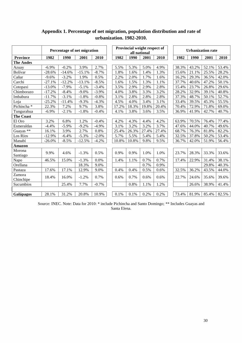
30

Appendix 1. Percentage of net migration, population distribution and rate of urbanization. 1982-2010.

Percentage of net migration

Provincial weight respect of all national

Urbanization rate

Province 1982 1990 2001 2010 1982 1990 2001 2010 1982 1990 2001 2010 The Andes Azuay -6.9% -0.2% 3.9% 2.7% 5.5% 5.3% 5.0% 4.9% 38.3% 43.2% 52.1% 53.4% Bolívar -28.6% -14.6% -15.1% -8.7% 1.8% 1.6% 1.4% 1.3% 15.6% 21.1% 25.5% 28.2% Cañar -9.6% -3.2% 1.9% 0.5% 2.2% 2.0% 1.7% 1.6% 16.2% 29.3% 36.5% 42.0% Carchi -27.1% -12.2% -13.1% -8.5% 1.6% 1.5% 1.3% 1.1% 37.7% 40.6% 47.2% 50.1% Cotopaxi -13.0% -7.9% -5.1% -3.4% 3.5% 2.9% 2.9% 2.8% 15.4% 23.7% 26.8% 29.6% Chimborazo -17.2% -8.4% -9.0% -3.9% 4.0% 3.8% 3.3% 3.2% 28.2% 32.9% 39.1% 40.8% Imbabura -11.7% -3.1% -1.8% -0.8% 3.1% 2.8% 2.8% 2.8% 37.3% 48.7% 50.1% 52.7% Loja -25.2% -11.4% -9.3% -4.3% 4.5% 4.0% 3.4% 3.1% 33.4% 39.5% 45.3% 55.5% Pichincha * 22.3% 7.2% 9.7% 3.8% 17.2% 18.3% 19.8% 20.4% 70.4% 72.9% 71.8% 69.0% Tungurahua -6.9% -2.1% -1.8% -0.4% 4.1% 3.8% 3.6% 3.5% 36.9% 41.9% 42.7% 40.7% The Coast El Oro 3.2% 6.8% 1.2% -0.4% 4.2% 4.3% 4.4% 4.2% 63.9% 70.5% 76.4% 77.4% Esmeraldas -4.4% -5.9% -9.2% -4.9% 3.1% 3.2% 3.2% 3.7% 47.6% 44.0% 40.7% 49.6% Guayas ** 16.1% 3.9% 2.7% 0.8% 25.4% 26.3% 27.4% 27.4% 68.7% 76.3% 81.8% 82.2% Los Ríos -12.9% -6.4% -5.3% -2.0% 5.7% 5.5% 5.4% 5.4% 32.5% 37.8% 50.2% 53.4% Manabí -26.0% -8.5% -12.5% -4.2% 10.8% 10.8% 9.8% 9.5% 36.7% 42.0% 51.9% 56.4% Amazon Morona Santiago 9.9% 4.6% -1.3% 0.5%

0.9% 0.9% 1.0% 1.0%

23.7% 28.3% 33.3% 33.6%

Napo 46.5% 15.0% -1.3% 0.0% 1.4% 1.1% 0.7% 0.7% 17.4% 22.9% 31.4% 38.1% Orellana 18.3% 9.0% 0.7% 0.9% 29.8% 40.3% Pastaza 17.6% 17.1% 12.9% 9.0% 0.4% 0.4% 0.5% 0.6% 32.5% 36.2% 43.5% 44.0% Zamora Chinchipe 18.4% 16.0% -1.2% 0.7%

0.6% 0.7% 0.6% 0.6%

22.7% 24.6% 35.6% 39.6%

Sucumbíos 25.4% 7.7% -0.7% 0.8% 1.1% 1.2% 26.6% 38.9% 41.4% Galápagos 28.1% 31.2% 20.8% 10.9% 0.1% 0.1% 0.2% 0.2% 73.4% 81.9% 85.4% 82.5%

Source: INEC. Note: Data for 2010: * include Pichincha and Santo Domingo; ** Includes Guayas and

Santa Elena.

31

Appendix 2. Definition and sources of variables

Variable Definition Source

Migration

People who changed residence in the 5 years prior to the Census of Population and Housing (CPV) (INEC, 2014), from the province of origin j to province of destination k

1982 : CEPAL – CELADE: 1990-2010: National Institute of Statistics and Census (INEC)

Population Number of people who live in the province j (L_Pop)

1974- 1982: hard copies of the census (CPV). 1990-2010: INEC

Rate of urbanization

Proportion of individuals who live in areas delimited as urban in each province (Urbanization rate)

1982: 1982: hard copies of the census (CPV). 1990-2010: INEC

Distance and time – 1

Kilometres (and time in minutes) from the capital of the province j to the capital of the province k (L Dist Y-P, L Time Y_P)

http://www.guiatelefonica.com.ec/Distancia_entre_ciudades_Ecuador

Distance and time – 2

Kilometres (and time in minutes) from the capital of province j to the capital of province k (L Dist Google, L Time Google)

Google Maps

Branch of activity of the economically active population (EAP)

Percentage of the economically active population that is employed in the following sectors: Agriculture, hunting, forestry and fishing (Agriculture); Mining and quarrying (Mines & Quarrying); Manufacturing industries (Manufacturing Ind); Other industries Industry Other); Construction (Construction); Services (Services).

1974-1982: hard copies of the census (CPV). 1990-2010: CPV – INEC

Level of education

Percentage of people who have completed no regular education level (No Education) primary education (Primary Education), secondary education (Secondary Education) and higher education, including postgraduate studies (Higher Education).

1974-1982: hard copies of the census (CPV). 1990-2010: CPV - INEC

Age Percentage of people by age groups. (Pop_0_4 … Pop_70 and over)

Census of Population and Housing, National Institute of Statistics and Census (INEC)

Category of employment

Percentage of people in each employment category: Employee (LM-Employee); Owner or partner (LM-Partner); Other form of employment (LM-Other)

1974-1982: hard copies of the census (CPV). 1990-2010: CPV - INEC

Characteristics of the dwelling

Characteristics of the conditions of the dwelling, used to construct the index of material welfare (Index Material WB)

1974-1982: hard copies of the census (CPV). 1990-2010: CPV - INEC