Micro-Loans, Insecticide-Treated Bednets, and Malaria: Evidence ...
Intermediated Loans: A New Approach to Microfinance∗
Pushkar Maitra†, Sandip Mitra‡, Dilip Mookherjee§
Alberto Motta¶, Sujata Visaria‖
May 2012Work in Progress: Comments Welcome
Abstract
This paper studies TRAIL, a variation on traditional microfinance, where a micro-finance institution appoints local intermediaries (traders or informal moneylenders)as agents to recommend borrowers for individual liability loans. There is no peermonitoring, group meetings or savings requirements. The loan duration is longer (4months) than in standard microfinance loans, designed to finance agricultural workingcapital. Borrowers who repay loans are eligible for larger loans in future loan cyclesand agents earn commissions that depend on loan repayments. We develop a modelof the credit market with adverse selection, in which borrowers vary with respect to(unobservable) project risk and (observable) landholdings, and the informal market islocally segmented. The model generates detailed predictions concerning informal in-terest rates, borrower selection, take-up and repayment patterns with respect to bothrisk and landholding categories. The predictions of the model are successfully testedusing data from a randomized evaluation currently being conducted in West Bengal,India, with traditional group-based joint liability loans (GBL) serving as the control.TRAIL is more successful in targeting low-risk clients, thereby generating higher re-payment rates, while GBL is more successful in targeting landless households. TRAILalso achieves higher take-up rates, suggesting that it manages to overcome problemsfaced by microfinance clients that are inherent in group-based lending and monitoring.
Key Words: Microfinance, Agent Based Lending, Group Lending, Selection, Takeup,Repayment
∗Funding was provided by AusAID under the ADRA scheme, International Growth Centre at theLondon School of Economics and the Hong Kong Research Grants Council’s General Research Fund.We are especially grateful to the staff of Shree Sanchari for their assistance in implementing the lendingschemes. Research assistance was provided by Clarence Lee and Moumita Poddar. Elizabeth Kwokprovided fantastic administrative support. We thank seminar participants at Monash University, ColumbiaUniversity and the University of Surrey and participants at the APEC Conference on Information andAccess to Markets at HKUST, the International Conference on Applied Microeconomics and DevelopmentEconomics at Kyoto University and the Workshop on Public Service Delivery in Developing Countries atth University of Bristol. The usual caveat applies.†Pushkar Maitra, Department of Economics, Monash University, Clayton Campus, VIC 3800, Australia.
[email protected].‡Sandip Mitra, Sampling and Official Statistics Unit, Indian Statistical Institute, 203 B.T. Road,
Kolkata 700108, India. [email protected].§Dilip Mookherjee, Department of Economics, Boston University, 270 Bay State Road, Boston, MA
02215, USA. [email protected].¶Alberto Motta, School of Economics, University of New South Wales, NSW 2052, Australia.
[email protected].‖Sujata Visaria, Department of Economics, Academic Building, Room 2340, Hong Kong University of
Science and Technology, Clear Water Bay, Hong Kong. [email protected]
1
1 Introduction
Over the last two decades microfinance is often regarded as a panacea for the problem of
low credit access by the poor. However despite the rapid growth in outreach of microfi-
nance institutions (MFIs), financial inclusion is far from universal, and a large proportion
of the world’s poor continue to be effectively excluded from credit markets. In partic-
ular, rigid, high-frequency repayment schedules and low tolerance for risk-taking have
meant that microfinance usually cannot be used to finance agriculture. In their book Poor
Economics, Banerjee and Duflo (2011) argue that the recent microfinance crisis in India
occurred partly due to the limited flexibility MFIs can afford with respect to repayments.
Karlan and Mullainathan (2010) argue that microfinance practitioners have been slow to
implement innovations in standard lending methodologies, which could explain why MFIs
have not yet reached a large proportion of the poor.1 In our field visits in West Ben-
gal, microfinance clients frequently mentioned the different limitations of microfinance:
restrictions on project choice; free riding within groups; contagious defaults; and harmful
effects on social capital. They also mentioned the high cost of attending weekly meetings
and achieving savings targets mandated by MFIs and the fact that no microfinance was
available for investment in agriculture.
These considerations motivated us to design a new approach to microfinance that seeks
to overcome the problems described above. In this approach loan duration matches the
agricultural production cycle, which allows the loans to be used for smallholder agricul-
ture. There is no collateral requirement, which makes the loans accessible to the very
poor. Individual liability loans are provided, thus avoiding problems associated with joint
liability. Savings requirements are dispensed with and groups play no role whatsoever.
At the same time, our approach continues to rely on utilization of local information and
social capital, the key basis of microfinance. Informed third-party individuals from the
local community, such as traders, shopkeepers, lenders or persons suggested by the local
village council are appointed by microfinance institutions as loan intermediaries. The loan
1The evidence on the importance of a rigid repayment schedule is however mixed. Field and Pande(2008) find that when they change the repayment schedule from every week to every month, there isno significant effect on client delinquency or default. They also find no evidence of the group meetingscontributing to higher repayment rates. On the other hand Feigenberg, Field, and Pande (2010) find thatfrequent interaction among group members builds social capital and improves their financial outcomes andthat clients who met more frequently were less likely to default in subsequent loan cycles.
2
intermediary (or agent) recommends borrowers for individual liability loans. The agent
is incentivized through commissions that depend on the loan repayment of the borrowers
they recommend. Restrictions are imposed on borrowers that can be recommended: they
are required to be landless or small/marginal landowners. The interest rate is pegged
below the average informal credit market rate. Borrowers have dynamic incentives to
repay: future eligibility for loans depends on repayment of the current loan, and loan offers
become larger progressively with successful repayment. The loan contract also provides
index insurance: repayment due is reduced in the event of village-level adverse shocks
to crop revenues. Some additional features reduce transactions costs for borrowers: the
MFI’s loan officers visit borrowers in their homes to deliver the loans; borrowers do not
have to attend mandated meetings with agents or MFI officers, or do not have to open
bank accounts.2 Both the transactions costs for borrowers and the administrative costs for
the lender are substantially lower as a result. We call this Agent Intermediated Lending or
AIL scheme. The TRAIL version of the program that we examine in this paper involves
the appointment of local traders as the agent.
We develop a theoretical model of borrower adverse selection to interpret the evidence,
and use the data to test its predictions. It extends Ghatak (2000), where borrowers
vary both with regard to (unobservable) riskiness of their projects as well as (observable)
landholdings. The informal credit market is characterized by segmentation wherein each
segment has a lender with exclusive information about the risk types of borrowers in their
own segment. This allows each lender to extract the surplus from safe borrowers in their
own segment, while competing with all other lenders in the village over lending to risky
types. The TRAIL version of AIL employs these same lenders as agents. While they are
best informed about riskiness of their own clients, they might also have an incentive to not
recommend their own low-risk clients for fear of losing their business. We seek to overcome
this incentive problem by introducing a repayment-based commission. The model predicts
that TRAIL agents select safe borrowers from their clientele if they do not collude with
the borrowers and the commission they receive is sufficiently high. In this case, they
recommend their own-segment clients who pay the lowest interest rate in the informal
market. These tend to be clients with an intermediate level of landholding. In contrast,
under the group based lending (GBL) scheme, clients who pay the highest interest rates
2These costs can be quite substantial for borrowers. See Park and Ren (200) for some evidence on thiscost.
3
in the informal credit market (who tend to have the lowest landholdings) who typically
self-select into the scheme. Additionally, GBL may attract risky as well as safe borrowers.
Hence the model predicts that (assuming the agents are suitably incentivized) the TRAIL
scheme generates superior targeting with respect to risk category of borrowers, while GBL
targets poorer clients. Empirically we expect TRAIL to achieve higher repayment rates,
while GBL is expected to be better targeted to the poor.
A complete welfare evaluation requires us to go beyond the standard performance metrics
that tend to be used by most MFIs, and focus also on impacts on the lives of the borrowers.
For any given client, TRAIL is predicted to generate higher benefits to borrowers on many
counts: they do not have to bear the burden of repaying on behalf of their group members
if they default. They also do not have to incur the costs of attending group meetings,
achieving savings targets, or face the problems of free-riding and social tensions that GBL
generate. Empirically, this should be manifested by higher takeup rates under TRAIL.
The predictions of our model are tested using data from a field experiment we are cur-
rently running in 72 villages in the Hugli and West Medinipur districts of West Bengal,
India. Starting in Fall 2010, Shree Sanchari (henceforth SS), an MFI that has been work-
ing in rural area of several districts in West Bengal, introduced one of three alternative
microcredit schemes in each of these villages. Two versions of the AIL scheme (TRAIL
and GRAIL) were each introduced in 24 villages. In TRAIL the agent is a trader in the
village; GRAIL is similar to TRAIL in all but one respect: in GRAIL the agent is recom-
mended by the village council (or the Gram Panchayat). For the purposes of this paper
we restrict ourselves to the analysis (and comparison) of TRAIL and GBL and leave the
analysis of GRAIL to future research.
In TRAIL, agents were selected from prominent traders in the village, who were asked to
recommend borrowers, and the MFI offered loans to a random subset of the persons rec-
ommended. Agents paid a small deposit to the MFI per recommended borrower who took
the loan. At the end of 4 months, repayments were collected and agents received commis-
sions equal to the interest earned, subject to a minimum repayment amount. Borrowers
were then eligible to take new 4-month loans of a larger size, subject to their repayment
behavior. In the remaining 24 villages SS introduced a group-based lending scheme similar
to the traditional microfinance model, with a few modifications: both men and women are
4
allowed to borrow, and the repayment duration is 4 months, to match the AIL schemes.
In the GBL scheme villages, villagers were invited to form joint liability groups, and 2
randomly chosen groups were offered loans. Groups followed savings requirements and
had mandated bi-monthly meetings with the MFI loan officers. At the end of 4 months,
repayments were collected and borrowers were eligible to take new loans of larger size,
subject to repayment.
The patterns of interest rates predicted by the model turn out to be borne out by the
evidence, and indicate that TRAIL agents were properly incentivized: they recommended
borrowers who were either their own clients or they had better information about (through
past interactions and/or through caste/religion networks). Those recommended by TRAIL
agents but unlucky in the lottery to receive a TRAIL loan turned out to pay an interest
rate substantially below those not recommended by the agent. GBL groups that formed
also tend to consist of safe borrowers compared with those that did not form groups,
judging by informal interest rates paid. Consistent with theoretical predictions, TRAIL
has achieved significantly higher repayment rates (exceeding 95%) than GBL (85%) at
the end of three repayment cycles. Selection across landholding levels also resembles
theoretical predictions: GBL groups consisted of the poorest clients (landless households),
whereas TRAIL borrowers tended to own between 0.5 to 1 acre. Finally, takeup rates are
slightly higher in TRAIL than GBL, and the difference has become statistically significant
from the fourth cycle onwards. In either case takeup rates in either scheme are above 80%.
These early results are encouraging: at the end of three loan cycles the schemes have
achieved high take-up and repayment rates, in a manner consistent with theoretical ex-
pectations. The agents appointed as intermediaries seem to have been incentivized by
the commissions to select safe types from among their clientele and the evidence does
not suggest collusive behavior. However a complete analysis of the comparative effects on
borrowers must also consider impacts on agricultural operations and incomes. To study
those we have to wait for the experiment to run its full course. We therefore defer a more
detailed analysis of borrower impacts to subsequent papers.
Our paper adds to the current (policy and academic) debate on individual versus joint
liability loans in microfinance. For example, the Grameen Bank in its Grameen II model,
Asa and BancoSol have adopted models of individual liability lending. There have been
5
several recent studies evaluating the relative merits and demerits of the two approaches. In
their study conducted in Philippines, Gine and Karlan (2010) find that moving from joint
liability contracts to individual liability contracts (or offering individual liability contracts
from scratch) did not change repayment rates. On the other hand, Attanasio, Augsburg,
Haas, Fitzsimons, and Harmgart (2011) from a study conducted in Mongolia find that
joint liability contracts have stronger effects on food consumption and entrepreneurship
(they attribute this to the disciplining effect of joint liability contracts).3 While under
TRAIL, households are provided individual liability loans, the contractual structure of
the loans making them very different from the individual liability loans discussed in At-
tanasio, Augsburg, Haas, Fitzsimons, and Harmgart (2011) and Gine and Karlan (2010).
The primary difference with respect to the former is in terms of collateral. In Attanasio,
Augsburg, Haas, Fitzsimons, and Harmgart (2011), the lender did not impose predeter-
mined collateral requirements but took collateral if available and in consequence 91% of
the individual loans were collateralized, with the average collateral value close to 90% of the
loan amount (page 15). This was contrary to the original microfinance objective of lend-
ing without collateral and implies that a large section of the population is either excluded
from the credit market or are severly rationed. TRAIL does not involve any collateral
requirements - it really is door-step banking and the household if recommended by the
village agent and selected for the loan, would be offered the loan. The second difference
is in terms of financial inclusion. In the individual lending program in Gine and Karlan
(2010), there is no specific collateral requirement, but all potential borrowers had to satisfy
a minimum savings requirement which could be used in the event the borrower failed to
repay. However the extent of financial inclusion is considerably lower. The loan officers
have a big role to play in deciding whether the bank should enter the community and
ultimately the bank entered only about 54% of the communities randomized. The center
size is significantly smaller on average for individual liability groups: this a consequence
of the unwillingness or inability of the loan officers to enter villages assigned to individual
liability. This imposes considerable restrictions on the specific individual liability lending
model. In TRAIL, the loan officers or the agents are local residents and therefore there is
no selection arising from the unwillingness or inability of external loan officers to entering
3Carpena, Cole, Shapiro, and Zia (2010) using data from a natural experiment from India where a MFIconverted individual liability loans to group liability loans, argue that group liability contracts improveupon individual liability, particularly in ensuring repayment and increasing savings discipline among clients.They argue that their results suggest a careful rethinking of such policy direction (page 4), where the policydirection in question is the move to individual liability contracts.
6
the community. Additionally there are no savings and collateral requirements.
2 Design
We conduct a randomized intervention in 72 villages in 2 districts (Hugli and West Me-
dinipur) of West Bengal in India. The intervention started in October 2010 and is expected
to continue until at least December 2012. The main credit intervention involves providing
agricultural loans, with repayment due in 4 months (120 days). Starting amount of loans
(in Cycle 1) was Rs 2000 but the loan amount increases with timely repayment. Specif-
ically the repayment amount (in each cycle) is 1.06× Outstanding loan. If the amount
due if fully repaid at the end of any cycle, loan offer in next cycle is 133% of that in the
previous cycle. For example a household that fully repays the amount due (initial loan of
Rs 2000 plus interest of 1.5 % a month) of Rs 2120 at the end of the 4 months following
the initial loan disbursement would receive a loan of Rs 2620 in Cycle 2. Borrowers who
repay less than 50% of the repayment obligation in any cycle are terminated and are not
allowed to borrow again; and if there is less than full repayment but more than 50% of
repayment, then the borrower is eligible for only 133% of the amount repaid. Cycle 1
started in October-November 2010, coinciding with planting of potato (the major cash
crop in this area).4 Borrowers are allowed to repay the loan in the form of potato bonds
rather than cash. In this case the amount repaid is calculated at the prevailing price of
potato bonds. While the loans are for agricultural purposes, households are not required
to document to the lender what the loan was actually used for. See Table 1 for more on
the credit program.
In TRAIL villages, SS employed a trader based in the local community as the agent -
only one agent was chosen per village. There were restrictions on who could serve as an
agent. Specifically traders who have at least 50 clients in the village, and/or have been
operating in the village for at least 3 years were given the first priority. Traders who have
fewer than 50 clients or have been working in the village for fewer than 3 years were given
the second priority and finally if an agent could not be obtained from either the first or
the second category of traders, others who come forward to participate as agents (they
4This happens to be the major potato growing region of India, producing approximately 30% of allpotatoes cultivated in India.
7
were given third priority). SS (in conjuction with village elders) created a list of traders
and randomly selected from this list. They approached the first randomly chosen trader
from this list and offered him the contract. If this trader refused to serve as an agent,
SS would go back to the list and randomly choose a second trader and approach him. In
practice the first trader who was approached always accepted the contract. The agent was
required to recommend names of 30 potential borrowers/households in the entire village.5
All recommended borrowers must be residents of the village and must own less than 1.5
acres of agricultural land. Landless households may be recommended. 10 out of these 30
recommended were randomly chosen and offered individual liability, 4-month (120 days),
low interest loan from SS.6
What are the agent incentives? Part of it is monetary. First, they would receive a com-
mission. 75% of all interest payment received would accrue to the agent as commission.
So at the end of Cycle 1 if all 10 households that received the loan repaid in full, the
agent would receive Rs 900 as commission. Second, there is a system of deposits and
bonuses aimed at ensuring that the agent recommends good borrowers. This works as
follows: the agent will be required to deposit Rs 50 per borrower with SS. This deposit
must be received by SS at the time the loans are sanctioned. The bonus is calculated as
follows: if the borrower repays x% of the loan, then the bonus equals x% of the deposit.
(For example, if the borrower repays half of the loan, and the deposit is Rs 500, then
the bonus is half of Rs. 500 = Rs. 250). The original deposit will be returned to the
agent at the end of 2 years (at the end of the 6th cycle), provided the agent has not been
terminated from the scheme. The actual program can however continue even beyond the
2 years. Finally agents (in conversations during field visits) noted that they expected to
increase their visibility within the village community and hence experience an increase in
market share. The other part of the incentives is non-monetary. First, at the end of 2
years the program will offer the agent and his/her family (up to 4 members) a special
holiday package in Puri or Digha (sea-side resorts near Kolkata, the capital of the state
of West Bengal), provided he has participated until the very end. Second, several agents
5Almost 96% of the TRAIL agents state trade/business as their main occupation and the agents areoverwhelmingly upper caste Hindus.
6In GRAIL villages, SS asked a member of the Gram Panchayat (village council) to make an informalrecommendation as to who could serve as an agent. The recommended individual needed to satisfy thefollowing criteria: must have lived in the village for at least 3 years; must have some personal familiaritywith small farmers in the village; and finally should be reputed to be a responsible person. Everything elsewas the same as in TRAIL.
8
view this activity as contributing towards an increase in their long term reputation within
the community and a boost to their ego.
Our idea that members of the local community could be employed to recommend and mon-
itor borrowers follows naturally from a large literature documenting the role of middlemen
and managers in contexts with asymmetric information problems (Melumad, Mookherjee,
and Reichelstein, 1995; Laffont and Martimort, 1998, 2000; Faure-Grimaud, Laffont, and
Martimort, 2003; Mookherjee and Tsumagari, 2004; Celik, 2009; Motta, 2011). Much of
this literature has found that the use of an informed third party as intermediary increases
the principal’s pay-off even if there is collusion between the intermediary and the agents
they supervise. Additionally, our AIL model resembles a lending approach that India’s
central bank has been promoting recently. With a view to increasing financial inclusion
for India’s rural population, the Reserve Bank of India has recommended that a network
of banking correspondents (BCs) and banking facilitators (BFs) be set up. The agents
in our model play the same role that the RBI envisions for BFs: they refer clients to the
formal lender, pursue the clients’ loan applications and facilitate the transactions between
the lender and the client. The final decision on whether to approve the loan rests with the
lender.7 There has been limited expansion of such programs in Thailand (Onchan, 1992),
Philippines (Floro and Ray, 1997), Bangladesh (Maloney and Ahmad, 1988), Malaysia
(Wells, 1978) and Indonesia (Fuentes, 1996).8 The framework is also similar to what
Floro and Yotopoulos (1991) refer to as credit layering, parallel to the distribution chain
in marketing. Our paper provides evidence from a randomized trial on the feasibility and
outcomes of such a scheme.
The trader-agent intermediated lending (TRAIL) treatment is compared to a Group Based
lending (GBL) model which uses the standard lending protocol used by SS (and indeed
almost all of the microfinance organizations in India): groups of size 5, joint liability and
initial savings requirement with one variation - repayment is due after 120 days and not
7Banking Correspondents (or BCs) on the other hand can disburse small loans and collect deposits aswell and they can make the final decision on whether to provide the loan or not. See Srinivasan (2008) formore detail.
8The programs were not particularly successful, even though given the complementarity between theformal and the informal financial sectors in the economy, this kind of programs could potentially increasecompetition in the formal financial sector. Floro and Ray (1997) argue that in the case of Philippines theproblem arose from the fact that the major group of informal lenders engaged in strategic cooperationthereby limiting competition. In the presence of this kind of anti-competitive behavior, programs thatpromote formal-informal sector linkages are open to extreme rent seeking behavior on the part of informallenders.
9
a fortnight after loans disbursed. This essentially implies that unlike in the traditional
model, the borrowers are able to invest in projects with a longer gestational period and
more importantly in agriculture, should they wish. Of the groups that were formed and
survived until the cut-off date of October 15, 2010, 2 were randomly selected via public
lottery. Members of the selected groups receive a total of Rs 10,000, which is divided
(typically equally) among the group members. They are joint liability loans of 4-month
duration, have similar dynamic lending criteria and have the same loan cycles as the agent
intermediated loans.
3 Data and Descriptive Statistics
We conduct an extensive household level survey of 50 households in each of the intervention
villages. The survey collects information on household demographics, assets, landholding,
cultivation, land use, input use, allocation of output, sales and storage, credit, incomes,
relationships within village. We plan to have 7 surveys over the period 2010 - 2012
(matching the credit cycles). Treatment households are recommended households that
receive loan (in TRAIL) or members of groups that are chosen to receive joint liability
loans (in GBL). Control 1 households are those that were recommended but did not receive
loan (in TRAIL) or members of groups that did not receive loans (in GBL). In each village
we also surveyed 30 households as additional control. These are the Control 2 households.
Table 2 presents the sample sizes of the Treatment, Control 1 and Control 2 households
in each of the sample villages. Each village is subject to only one treatment and we refer
to villages that receive the TRAIL (GBL) treatment as TRAIL (GBL) villages.
Villages were randomly allocated to the treatment. Table 3 shows that at the village
level, there are no significant differences in village size, number of potato cultivators in the
village and the number of potato cultivators in the different landholding categories across
the two treatment groups: the differences TRAIL − GBL is never statistically significant.
In terms of household characteristics, comparison across the different treatments is not
so easy. This is because there is a process of selection involved (recommendation in
TRAIL and group formation in GBL) and so the sample of household in each village
is not random. We instead restrict ourselves to a random set of households selected in
10
2007-2008 as a part of a different and related project conducted in these village (see
Mitra, Mookherjee, Torero, and Visaria, 2012, for more details). This sample was selected
long before the credit interventions were introduced in these villages. There are a few
systematic differences in terms of the household characteristics in the TRAIL and GBL
villages; crucially households in TRAIL villages report far greater interactions with the
agent compared to interactions with the group leaders in GBL villages.
The process of selection is very different in TRAIL and GBL and this becomes clear when
we compare the average characteristics of the recommended/selected households in TRAIL
and GBL (Table 4). The selection process in TRAIL is significantly less pro-poor compared
to GBL: the average level of landholding is significantly higher in TRAIL recommended
households, while households that select into groups in GBL are significantly more likely to
be landless. Prior interaction between the agent and the TRAIL recommended households
is significantly greater compared to the prior interaction between the group leader and the
GBL selected household.
How different are TRAIL and GBL selected households compared to the average house-
hold? To examine this, Table 5 compares the means and standard errors of the selected
households to the average household (defined by the 2007-2008 sample). Recommended
households in TRAIL have greater prior interaction with the agent relative to a randomly
selected household in the same village; TRAIL and GBL selected household have less
landholding compared to the sample average. This is due to the experimental design −
the credit intervention was restricted to households with at most 1.5 acres of land. On
the other hand TRAIL and GBL selected households are more likely to have received GP
benefits. All of this suggests that selected households are poorer compared to the village
averages. Targeting has indeed worked.
The majority of loans are from traders (see Figure 1) - 56% for the full sample, followed by
cooperatives (12.6%) and SS (11%). There are some interesting differences across the two
districts - the fraction of loans from the trader is higher in West Medinipur (58%) compared
to Hugli (54%) and this is balanced by the fact that borrowing from the cooperative is
higher in Hugli, relative to West Medinipur. The average interest rate and the size of the
loan varies significantly across the different lender categories. Interest rate varies from
almost 34% per annum for borrowing from the money lender to 10.5% per annum for
11
borrowing from the bank. Also interesting is that while only 3.5% of all loans are bank
loans, the average amount of bank loans is more than Rs 31,000. It appears that while
formal sector (bank) loans are difficult to obtain, if they can be obtained, the loan amount
can be substantial.
Before proceeding further, it is worth discussing the relationship between landholding and
the interest rate that households have to pay on loans from informal sources and on the
relationship between landholding and project returns. These empirical relationships have
implications on the assumptions that we make in the model (in Section 4). First, Figure
2 presents the predicted value of interest rate in the informal market on landholding and
shows that there is a u-shaped relationship between interest rate in the informal market and
landholding. Second, this u-shaped relationship suggests that project returns are convex
in the level of landholding. Table 6 presents evidence in support of this. Project returns
(here defined as crop profit from potato cultivation) is indeed convex in the amount of
landholding. This effect persists even when we control for the variety of potato cultivated
(column 2).
4 The Model
In this section we develop a theoretical framework to highlight the particular characteris-
tics of the AIL scheme. To compare more effectively with the commonly used microfinance
models, we build on Ghatak (2000). The action in that model stems from the combina-
tion of asymmetric information and lack of collateralizable wealth. Borrowers have some
information about the riskiness of each other’s projects that lenders do not. All projects
require one unit of capital but a safe project has probability of success ps ∈ (0, 1), which
is strictly higher than the probability of success of a risky one, pr. If a lender cannot
identify a borrower’s type then they have to offer the same interest rate to all borrowers.
Owing to limited liability and the lack of collateralizable wealth, borrowers repay the loan
only if the project is successful. Hence, a lender dislikes risky borrowers whose repayment
rates are inherently low. As a consequence, the interest rate in the credit market rises.
If the interest rate ends up being high enough, the safe borrowers might decide not to
borrow even if their project would make a positive contribution to social surplus. This is
known as the under-investment problem in credit markets with adverse selection (Stiglitz
12
and Weiss, 1981). Ghatak (2000) shows that adopting a GBL scheme, a lender can utilise
information borrowers may have about each other and achieve high repayment rates. It
does so by offering a menu of contracts and allows individuals to self select.
How does GBL compare with AIL in such a context? To answer this question and to
accommodate the peculiar features of AIL, we need to extend Ghatak (2000). In his
model all lenders are equally uninformed, so local lenders have no additional information
about risk types of borrowers, compared with external lenders. In practice, local lenders
have extensive past experience in lending to their respective clienteles and have thereby
accumulated substantial knowledge about their relative reliability in repaying loans. This
is exactly the comparative advantage of local lenders vis-a-vis external lenders, which
makes it difficult for formal financial institutions with access to capital at lower costs from
driving local lenders out of business. To accommodate this we need to allow local lenders
to have better information about risk types of local borrowers they have dealt with in the
past, compared to other lenders who do not have that experience.
We therefore posit that local credit markets are segmented, with each segment occupied by
one lender who lends habitually to borrowers in that segment and thus comes to learn their
respective risk types. This information is not available to lenders in other segments of the
market. Lenders therefore acquire a measure of monopoly power within their respective
segments as a result of their ability to discriminate between safe and risky types from past
experience. All segments involve the same ratio θ of risky to safe types of borrowers.
The other direction we extend the Ghatak model is to introduce an additional dimension
of heterogeneity, with respect to level of landholding a ≥ 0 of each borrower. This char-
acteristic is observable. This is necessary to examine the relative success of AIL and GBL
with respect to targeting poor versus very poor borrowers.
To keep the analysis simple, we preserve other aspects of the Ghatak model. All borrowers
and lenders are risk neutral. Lenders face no capacity constraints and have the same cost ρI
per unit of money loaned. All projects involve a fixed scale of cultivation with a given need
for working capital, so loan sizes do not vary.9 Let the scale of cultivation be normalized
9The model can be extended to allow for variable scale of cultivation and thereby variable loan sizes.Although the results would remain qualitatively similar to the ones presented here, the analysis wouldbecome considerably more complicated.
13
to one unit of land, and the required loan size to one rupee. If a < 1, the borrower needs
to lease in 1 − a in order to cultivate. Project returns will be assumed to be increasing
in a, owing to the reduction in distortions associated with tenancy, ranging from inferior
quality of leased in land to Marshallian undersupply of effort.10 If successful, a borrower
of type i ∈ {r, s} with landholding a obtains a payoff Ri(a). Additional assumptions on
this payoff will be provided below. We also make the simplifying assumption that the
probability of success is independent of landholding.11
Higher landholdings are also associated with a higher autarkic outside option, should the
farmer in question decide not to pursue the cultivation project. For instance, the owner
of the land always has the option of leasing it out. It is reasonable to suppose that the
outside option is linear in a. We normalize and postulate that the outside option equals
a.
Using his privileged information, a lender operating in any given segment can make per-
sonalized offers to her own clients. But he can also try to attract borrowers belonging
to other segments. Since loan sizes do not vary, the terms of the loan are summarized
entirely by the interest rate. A contract Γ = {rs(a), rr(a), r(a)} specifies the interest rates
respectively for own-segment safe borrowers, own-segment risky borrowers, and other-
segment borrowers, for any given landholding a. Interestingly, the same conditions that
give rise to the asymmetric information problem in Ghatak (2000) also ensure existence
of an equilibrium in the segmented informal market. These conditions are
Rr(a)− a
pr≥Rs(a)− a
ps(1)
Rs(a)− a
ps<ρIp
(2)
psRs(a) >ρI + a (3)
where equation (1) ensures that any interest rate that satisfies the safe borrowers’ par-
ticipation constraint also satisfies the risky borrowers’ participation constraint (i.e., there
is no interest rate that attracts only safe borrowers); equation (2) implies that the par-
10Tenurial laws in West Bengal mandate tenants’ share should be at least 0.75, unless the landlord sharesin provision of material inputs in which case they share 50 : 50 in both inputs and outputs. The latterarrangement is rare, as most landlords are not involved in cultivation (see for example Banerjee, Ghatak,and Gertler, 2003)
11This assumption can be relaxed at the cost of increasing the complexity of the analysis and weakeningthe sharpness of the predictions. Moreover, the data shows no tendency for loan repayment rates to varywith landholdings.
14
ticipation constraint of safe borrowers is not satisfied when the interest rate, r, is greater
or equal to ρI/p, with p ≡ θpr + (1 − θ)ps; equation (3) entails that the safe project is
socially productive. If the lenders charge all borrowers the same interest rate r, and both
types of borrowers borrow in equilibrium, the lenders need to charge at least r = ρI/p
to break even. Hence, from equation (1) and equation (2) follows that there does not
exist a pooling contract that attracts both types of borrowers and satisfies the break even
condition of the lenders. The only possible individual liability contract then is the one
that attracts risky borrowers.
Condition equation (3) implies that safe borrowers would make a positive contribution to
social surplus. Hence, the equilibrium in the informal market where only risky borrowers
borrow is socially inefficient. The repayment rates and welfare are strictly less than that
under full-information.12
Why are these conditions necessary for the existence of an equilibrium in the informal
market? Owing to her privileged information, an informal lender can identify her safe
clients and offer them an interest rate low enough to convince them to accept (the safe
project is after all socially productive, so such an interest rate exists), but high enough to
extract all their surplus. The asymmetric information problem is assumed to be severe and
therefore the other lenders are not willing to compete for these safe clients because it is not
possible to attract them without attracting the risky clients as well. Hence, asymmetric
information shields the lender from the competition. This result is encapsulated in the
following Lemma. The formal proof is presented in the Appendix.
Lemma 1 In equilibrium, the safe borrowers do not borrow from other-segment lenders.
Using Lemma 1 it is possible to show that there is a unique equilibrium where the lenders
offer a relatively low interest rate to their safe clients, and extract all their surplus. In
equilibrium, the lenders also offer a relatively high but fair interest rate to their risky
12Note that our model is also equipped to deal with the over-investment problem analyzed in Ghatak(2000). In the over-investment case equation (1) and equation (3) hold but equation (2) doesn’t. Inaddition we need prRr(a) < ρI + a to ensure that the risky project is socially unproductive. Then thereis a pooling contract that attracts both types of borrowers and satisfies the breakeven condition of thelenders. But this is an inefficient outcome for society because the risky project should not be financed.Risky projects thrive only because they are cross-subsidized by the safe ones. Under these circumstances,we prove in Proposition 2 that an equilibrium in the informal credit market does not exist.
15

clients. This is the result of the competitive tension between different lenders who actively
attempt to undercut each other. Proposition 2 presents this result more formally:
Proposition 2 There is a unique equilibrium outcome in the informal market, in which
safe types owning land a borrow from their own-segment lender at interest rate rs(a) ≡
Rs(a)− aps
, while risky types borrow (from any lender) at interest rate rr ≡ ρIpr
which does
not depend on their landholding.
It is worth noting that the equilibrium interest rate for the risky borrowers is higher than
the one for the safe borrowers (owing to (A2)). Moreover, the former does not depend
on the level of landholding. On the other hand, the interest rate for the safe borrowers
depends on the level of landholding. The nature of this relationship depends on the shape
of the return function Ri(a): it is rising or falling in a depending on whether R′i(a) exceeds
or falls below 1ps
. If Ri(a) is convex in a, the interest rate is likely to exhibit a u-shape. As
we have already seen in Table 6, the evidence does support this assumption. The model
thus provides an explanation of the observed u-shape of the interest rate.
The u-shaped interest rate curve in Figure 3 has an intuitive interpretation: It can be
seen as the surplus that the lender extracts from his safe clients. Initially the surplus is
large because the lender is in a strong bargaining position owing to the client’s outside
option, a, which is low. An increase in a boosts the value of the project, and consequently
the surplus that the lender can extract. But it also increases the client’s outside option,
weakening the bargaining position of the lender. If Ri(a) is convex, the second effect could
dominate for low values of a, while it would be dominated for high values of a.
Note also that (3) implies that safe types will operate the project, irrespective of their
landholding. On the other hand, risky types may or may not participate at any given level
of landholding, depending on how Rr(a) − apr
relates to ρIpr
. Figure 4 depicts a possible
scenario where the risky project has higher returns than the safe one, but it is not socially
productive for low values of a. This case is consistent with a situation where participation
rates for risky types increase rapidly with landholding for low values of a and stabilize
afterward. The overall pattern of interest rates that would be observed in the informal
market would then flatten out (or even rise) once risky types enter the market. Once they
have all entered, the u-shaped pattern will then resume.
16
Finally, note that the payoff in the informal credit market represents the outside option
for borrowing from external lenders. For a borrower of type (i, a), let us denote this
outside option by ui(a). Proposition 2 implies that borrower (s, a) obtains a payoff equal
to a, whereas a borrower (r, a) obtains a positive payoff prRr(a) − ρI > a. Lenders
make positive profits on their own-segment safe borrowers. In equilibrium Πr(a) = 0 and
Πs(a) = psRs(a)− ρI − a, where Πi(a) denotes the profit from borrower (i, a).
4.1 Implications of GBL
Now suppose an MFI enters and offers joint liability loans to qualifying groups of borrow-
ers. In order to benchmark AIL against GBL, we revisit Ghatak (2000) in light of the
endogenous outside options analyzed in the previous section. As in Ghatak we simplify
and assume that GBL requires the borrowers to form groups of two: there is an individual
liability component, r, and a joint liability component, c. Limited liability still applies,
but if a borrower’s project is successful, and the other member of the group fails, the
former has to pay the additional joint liability component, c. The contracting problem
is the following sequential game: first, the bank offers a finite set of joint liability con-
tracts {(r1(a), c1(a)), (r2(a), c2(a)), ...}; second, borrowers who wish to accept any one of
these contracts select a partner and do so; finally, projects are carried out and outcome-
contingent transfers as specified in the contract are met. Borrowers who choose not to
borrow enjoy their reservation payoff of ui(a). Instead of looking at the optimal joint
liability contract we take r(a) = c(a) = rT as given and we study the impact of this
group loan on the credit market.13 Further, borrowers have to attend group meetings,
and meet saving requirements in order to qualify for a group loan. This imposes cost γi
for risk type i. Ghatak (2000) proves that any joint liability contract (r, c), with r > 0
and c > 0, induces assortative matching in the formation of groups. This result extends
to our framework: the borrowers that self-selected in a group are of the same risk type.
The expected gain for type (i, a) from a group loan instead of the informal market loan is
Ui(rT , a)− ui(a) = pi [Ri(a) + (pi − 2)rT ]− γi − ui(a). (4)
13Without loss of generality Ghatak (2000) restricts attention to the set of contracts which have nonnegative individual and joint liability payments, FJL = {(r, c) : r(a) ≥ 0, c(a) ≥ 0}. Gangopadhyay,Ghatak, and Lensink (2005) shows that ex-post incentive-compatibility requires r = c. Accordingly theyfurther restrict attention to the set FJL = {(r, c) : r(a) = c(a) ≥ 0}.
17

The borrowers accept the group loan if the above expression is positive and the limited
liability constraint is satisfied:
2rT ≤ Ri(a), i = r, s. (5)
For a safe type borrower with land a, this expression reduces to
Us(rT , rT , a)− us(a) = ps[rs(a)− (2− ps)rT − γs] (6)
which implies that the gain is higher if the borrower faces a higher interest rate in the
informal sector. Among safe types, therefore, we expect higher participation rates from
those landholdings that correspond to higher interest rates.
For a risky type borrower who participates in the informal market, the gain is
Ur(rT , a)− ur(a) = ρI − pr(2− pr)rT − γr (7)
the difference between the expected interest costs, less the cost cr of qualifying for the
group loan. This expression is independent of a. On the other hand, for a risky type
borrower excluded from the informal market the gain is
Ur(rT , a)− ur(a) = prRr(a)− a− pr(2− pr)rT − γr (8)
which is likely to vary with a in ways that depend on the curvature of Rr.
The relative benefits from a group loan for safe and risky types (for given a) are also
ambiguous. Safe types could gain more as they earn a lower payoff in the informal market.
On the other hand, their expected repayment is higher. To see this, rearrange equation
(4) and compare the gains of two borrowers (s, a) and (r, a):
psRs(a)− prRr(a)︸ ︷︷ ︸ambiguous
+[(2pr − p2
r)− (2ps − p2s)]rT︸ ︷︷ ︸
negative (by assumption)
+ γr − γs︸ ︷︷ ︸ambiguous
+ ur(a)− us(a)︸ ︷︷ ︸,non-negative (in equilibrium)
4.2 Agent-Intermediated Lending: TRAIL
Under TRAIL, the contracting problem is as follows: first, the bank offers a contract
(rT ,K) to the informal lender or the agent/intermediary; second, the lender recommends
a borrower who either accepts or refuses the loan; finally, projects are carried out and
18
outcome-contingent transfers as specified in the contract are met; the borrower repays
rT if the project is successful and zero otherwise; the lender obtains a fraction K of the
repayment, rT . Borrowers who choose not to borrow receive their reservation payoff of
ui(a). We take rT and K as given and we study the impact of this loan on the credit
market.
Suppose the agent and the borrowers (he recommends) play non cooperatively. The
lender’s expected commission from recommending the own-segment safe borrower isKpsrT .
This is higher than the expected commission from other-segment borrowers, KprT , which
is in turn higher than the commission from recommending the own-segment risky borrower,
KprrT . The opportunity cost of recommending risky and other-segment borrowers is zero,
ensuring that the latter option is always preferred by the lender. On the other hand, rec-
ommending the own-segment safe borrower entails losing the opportunity to serve her in
the informal market, and to earn the associated profit Πs(a). Note that the lender can
minimize the opportunity cost Πs(a) by selecting a safe client with a suitable level of land-
holding. The level of landholding which minimizes Πs(a) is a∗ = arg min rs(a) ≡ Rs(a)− aps
,
i.e, the landholding corresponding to the lowest interest rate for a safe type borrower. It is
optimal for the lender to recommend own-segment safe borrowers (s, a∗) if the commission
rate is high enough to outweigh the foregone profits from lending to a∗:
K ≥ psRs(a∗)− ρI − a∗
rT (ps − p)≡ K (9)
The borrower (i, a) accepts the offer if the MFI interest rate is lower than the one in the
informal market, i.e., the rT ≤ ri(a). In what follows, we make the following assumption.
Assumption 1: rT is lower than the maximum interest rate offered in the informal mar-
ket.
This assumption is consistent with our data. It implies that it is always profitable for the
lender to recommend some borrower. The following proposition summarizes these results:
Proposition 3 Suppose Agent-Intermediated Lending is not subject to collusion.
a) If K ≥ K, lenders recommend own-segment safe borrowers with a level of landholding
corresponding to the lowest informal sector interest rate such that rs(a) ≥ rT .
19
b) If K < K or rT > r∗s(a) for all a, lenders recommend other-segment borrowers with
any level of landholding.
Now consider what happens when AIL is subject to collusion. The collusion process is
modelled as follows: the lender makes a take-it-or-leave-it offer to the borrower. This
offer requires the borrower to pay a bribe b in exchange for being recommended. If the
borrower refuses the offer, the game is played non-cooperatively. The lender keeps in mind
that he must leave the borrower with at least the same level of utility she would obtain
by rejecting the collusive offer, i.e., ui(a). It turns out that:
Proposition 4 If Agent-Intermediated Lending is subject to collusion, it is never optimal
for a lender to recommend own-segment safe borrowers. On the other hand, it is always
optimal to recommend a borrower from other segments. In some circumstances it can
also be optimal to recommend risky borrowers in one’s own segment with any level of
landholding.
The intuition behind this Proposition is the following. Given that the lender has all the
bargaining power, he can extract the entire surplus generated by the AIL recommendation.
This is achieved by asking a bribe that leaves the borrower with exactly the same level
of utility she would obtain by rejecting the collusive offer. When it comes to the own-
segment safe borrower, the lender becomes effectively the residual claimant of the project.
The lender obtains a gain equal to KpsrT +ρI−psrT = ρI−(1−K)psrT by recommending
the own-segment safe borrower. Analogously the gain from recommending an own-segment
risky type is ρ− (1−K)prrT . These are the saving of the lender’s cost of capital ρI as the
borrower switches to borrowing from the MFI, less the net expected repayment (1−K)pirT
by the coalition of the lender and the borrower type i. The expected repayment is lower
for the risky type. Hence the agent prefers to recommend a risky rather than safe type
from his own segment. Selecting safe clients is never optimal, in stark contrast with the
no-collusion case.
But an even more attractive option is to report other-segment farmers. If possible, it is
optimal for the lender to ask a bribe that attracts only the safe borrowers from other
segment. Denote this by option (i). This is the first-best option for the lender because
20
it combines high expected commission with zero opportunity cost. If this option is not
available the lender considers two alternatives: (ii) ask a bribe that attracts both the
risky and safe borrowers from other segments or (iii) ask a bribe that attracts only the
risky borrowers. The trade off is between obtaining a higher expected commission (that
is, KprT instead of KprrT ), and setting a lower bribe, which is required to attract both
risky and safe borrowers from other segments. If option (i) or (ii) is selected, the lender
recommends other-segment borrowers with level of landholding such that psRs(a) − a is
maximized. In option (i) this comes from the fact that the lender is the residual claimant
of the project and wants to maximize the expected returns. In option (ii) this result is due
to the fact that the lender tries to maximize the bribe. There can also be circumstances
where option (iii) is best, which explains the last statement in the Proposition.
4.3 Summary of Theoretical Predictions
The predictions of the TRAIL model depend on whether agents collude with borrowers,
and also on the size of the commission. Say that TRAIL is effective if there is no collusion
and K > K. In that case, the agent recommends safe types paying the lowest informal
interest rate (among those for whom this interest rate is higher than the AIL interest
rate). And if TRAIL is not effective, then the agent recommends more risky clients.
This indicates a way of testing whether TRAIL is effective. First check whether the
average interest rate on informal loans paid by Control 1 households (those recommended
by the agent but did not receive the loan under this scheme) is systematically lower than
that faced by Control 2 households (who were not recommended by the agent). We need
to exclude Treatment households (those who were recommended by the agent and were
randomly selected to receive credit) from the analysis here because the very fact that these
households received low interest loans from SS due to agent recommendation could mean
that their type becomes public within the community. They might now have access to low
interest informal loans, which they would not have otherwise. Additionally we can check
whether
a. the agent actually uses the information on interest rates paid (i.e., knowledge about
the type of the borrower) in the recommendation process; and
21
b. they exhibit a bias in favor of recommending clients on whom they have more in-
formation, either through prior economic interactions or through caste and religion
networks.
Assuming that this test for effectiveness is passed. Then we expect the following differences
between TRAIL and GBL:
Targeting: TRAIL selection will be biased in favor of those paying the lowest interest
rates in the informal market (subject to the constraint of the TRAIL rate being
lower than the average informal rate, which is true). This corresponds to households
with an intermediate level of landholding. In contrast GBL selection will be biased
in favor of landless households (paying the highest average informal interest rate).
Takeup: Controlling for landholding, takeup rates should be higher under TRAIL, since
TRAIL clients incur a lower repayment burden and avoid the cost of attending
meetings and achieving savings targets.
Repayment: TRAIL should achieve higher repayment rates than GBL.
5 Results
Are the predictions regarding selection, takeup and repayment validated empirically? To
answer this question we examine the evidence on selection/recommendation of clients and
on takeup/continuation and repayment over the first year of this ongoing project. In our
empirical analysis we use non-parametric plots and regressions which control for household
characteristics and village fixed effects.
TRAIL effectiveness
The basic premise of the TRAIL model is that the agent has information on the type of the
borrower and will use this information to recommend safe (own segment) borrowers. The
interest rate paid by households on informal loans is a measure of the innate riskiness of
the borrower. If TRAIL is effective, then the agent will recommend his own segment safe
types. To see if this is true, we compare the interest rates on informal loans (excluding
22
loans from friends and family) paid by Control 1 households to that paid by Control
2 households. If TRAIL is effective then the average interest rate paid by Control 1
households should be significantly lower than that paid by Control 2 households. This
is clearly true irrespective of the level of landholding (see Panel A, Figure 5). This is
further supported by the regression results presented in column 1, Table 7: controlling
for landholding, Control 1 households pay a significantly lower interest rates on informal
loans, compared to Control 2 households.
Next we seek an answer to the question: do agents exhibit bias towards own segment safe
clients? To do this, we examine the effect of risk types and prior interactions between the
agent and the household on the likelihood of being recommended. We define a dummy
variable Prior Interaction, which takes the value of 1 if the agent has previously interacted
with the household (the household has previously bought from the agent or borrowed from
the agent or worked for the agent) and interact this variable with risk type of the household
captured by the average interest rate the household pays on informal loans. We define two
dummies to capture the risk type of the household: Average Interest Low if the average
interest rate on informal loans is less than 18% and No informal borrowing if the household
did not borrow from informal sources in the three months prior to the survey. This could
of course mean either that the household voluntarily chooses not to borrow from informal
sources or are excluded (involntarily) from the informal market. However it does imply
that in this case the risk type of the household cannot be determined.
The regression results are presented in Table 8. In all the regressions we control for
landholding. The results in column 1 support our hypothesis of the agents being biased in
favor of households who have prior interactions with the agent - prior interaction increases
the likelihood of being recommended by 15 percentage points. The results in column 2
support the hypothesis that the agent chooses to recommend safe households: households
with low average interest rate are 77 percentage point more likely to be recommended.
The coefficient estimate associated with prior interaction becomes slightly weaker when
we include the risk type dummies (column 3), but it continues to remain statistically
significant. Overall however the information on the risk type of the household appears to
be more important than prior interaction. The difference estimates Prior Interaction ×
No Informal Borrowing and Prior Interaction × Average Interest Low is never statistically
23
significant. Irrespective of prior interaction, households that are able to borrow at a
lower interest rate from the informal market are more likely to be recommended and prior
interaction has no additional effect on the likelihood of being recommended. Columns 5
and 6 builds on this by successively adding additional networks. Agents belonging to high
caste are significantly less likely to recommend scheduled caste (SC) households; Hindu
agents are less likely to recommed non Hindu households; agents exhibit a slight bias in
favor of households where the primary occupation is labor.
All of this suggests that TRAIL is indeed effective.
The patterns of group formation under GBL reveal an interesting pattern. Remember
Control 1 households in GBL villages are those who select themselves into groups but
do not receive the SS loan. So the interest rate paid on informal loans by Control 1
households is a measure of the riskiness of the group members. While theoretically it is
possible for groups to comprise of both risky and safe types (and this, we argue theoretically
contributes to a lower repayment rate in GBL), we see that Control 1 households in TRAIL
and GBL pay very similar interest rates on informal loans. This appears to suggest that
there is assortative matching by type in groups (as in Ghatak, 2000): risky households are
excluded from groups; safe households self select into GBL and risky households borrow
from the informal market at higher interest rates. See Panel B in Figure 5 and further
support from the regression results presented in column 2 in Table 7.
Targeting by Landholding: Selection/Recommendation
Overall around 96% of households who were recommended/formed a group owned no
more than 1.5 acres of land. This requirement was imposed on the agents and in the
group formation process in TRAIL and GRAIL. The corresponding proportion was around
81% for the Control 2 (non-recommended/non-selected) households. Here sampling was
conducted on the basis of the land distribution at the village level. There is no difference
in the proportion of households that do not satisfy the landownership criterion across
the different treatment groups. In analyzing selection we therefore restrict ourselves to
households owning no more than 1.5 acres of land.
The theoretical model predicts that TRAIL selection will be biased in favor of those
24

paying the lowest interest rates in the informal market, subject to the constraint that the
interest rate offered under TRAIL is lower than the informal rate (i.e., households with
an intermediate level of landholding). In contrast GBL selection will be biased in favor
of landholdings exhibiting the highest average informal interest rate (i.e., the landless
households).
Figure 6 presents the lowess plots of the likelihood of being recommended (or choosing
to form a group) on landholding. There is an inverted u-shaped relationship between the
likelihood of being recommended in TRAIL and landholding, with the likelihood of being
recommended highest in the intermediate landholding range. The pattern of recommen-
dation in TRAIL is consistent with the agent recommending his own segment safe types,
those who pay lower interest rates in the informal market. That said, the peak of the
likelihood of recommendation is attained at a level of landholding of around 0.5 acres,
slightly higher than the size (0.3 acres) associated with the lowest interest rate (Panel A
in Figure 5). The likelihood of group formation (in GBL) decreases monotonically with
an increase in landholding, indicating that GBL is more pro-poor.
These non-parametric patterns are corroborated in the regression results presented in
Table 9. These are reduced form regressions for the likelihood of being recommended in
TRAIL and the likelihood of forming a group in GBL. Consistent with the lowess plots
in Figure 6, there is an inverted u-shaped relationship between landownership and the
likelihood of the household being recommended. The probability of being recommended
by a TRAIL agent is highest for households owning approximately 0.5 acres of land. In an
alternate specification we included a landless household dummy (as opposed to continuous
landholding and landholding squared). The landless dummy was not significant in the
recommendation regression for TRAIL, but landless households are significantly more
likely to select themselves into groups under GBL.
There is also evidence of biases in favor of recommending borrowers from specific reli-
gion, caste and occupation groups in TRAIL. This has already been reported in the test
for TRAIL effectiveness (Table 8). Hindu TRAIL agents were significantly less likely to
recommend a non-Hindu household. In the case of TRAIL agents who are businessmen
exhibited a slight bias in favor of households where the primary occupation of the house-
hold head is labor. Finally, prior interaction with the agent (bought from agent, borrowed
25
money from agent and worked for agent to a lesser degree) significantly affected the likeli-
hood of being recommended. In the case of GBL, prior interaction with the group leader
(in the form of borrowing from the group leader) significantly increases the likelihood of
being a part of a group. This is partly a result of the specific model of microfinance that
is adopted by many MFIs in India where the group leader is chosen first, who then has
some say in inviting other members into the group.
Takeup
Controlling for landholding, takeup rates should be higher under TRAIL, since TRAIL
clients incur a lower repayment burden and avoid the cost of attending meetings and
achieving savings targets. Figure 7 presents the takeup rate in Cycle 1 and the likelihood
of continuation in subsequent cycles (this of course depends on repayment in the previous
cycle and the willingness to re-borrow). There is no particular pattern in the (conditional)
takeup rates in the two treatments across the different cycles, conditional on eligibility.
Table 10 presents the linear probability regressions for loan takeup in Cycle 1. There is,
as one would expect from Figure 7, no difference in the takeup rate between TRAIL and
GBL. The takeup rate is significantly lower in Hugli (driven by TRAIL). This last result is
interesting as it corroborates the anecdotal evidence obtained from field visits that suggest
that access to microcredit is significantly higher in Hugli, which is closer to Kolkata (the
state capital) and demand for additional credit is significantly lower in Hugli. The results
are robust to the presence of other MFIs in the village and the intensity of microfinance
activity in the village.
This Hugli effect persists over time and indeed becomes stronger. Table 11 presents the
linear probability regression results for continuing to borrow in Cycles 2 (column 2), 3
(column 3) and 4 (column 4), conditional on eligibility. For comparison purposes we also
include the results from takeup in cycle 1. Both the takeup and continuation probabilities
are lower in Hugli compared to West Medinipur and this difference becomes stronger over
the first three cycles (increasing from 14 percentage points in cycle 1 to 20 percentage
points in cycle 3), though falls in cycle 4 (down slightly to 15 percentage points, still
statistically significant). There is no statistically significant difference in the takeup rate
between TRAIL and GBL. Landholding has no effect on takeup/continuation rate in any
26
cycle. Again the results are robust to the inclusion of intensity of microfinance activity in
the village and presence of other MFIs in the village.
However these household level regressions do not tell the full story. If we are interested in
overall financial inclusion, then we would like to know what proportion of the maximum
eligible actually receive the loan in each cycle. Ideally one would want everyone eligible
to receive the loan i.e., takeup rate to be 100%. However takeup rate in is considerably
less than 100% in all the cycles. This is partly voluntary (some households chose not
to borrow) and partly involuntary (households could not borrow because they could not
repay their existing loans) and in some cases groups did not survive. In Figure 8 we present
the average proportion of eligble households actually receiving the loan in each cycle, by
treatment. While the proportion of households receiving the loans is always higher in
TRAIL, the difference is only statistically significant in Cycle 4. This is corroborated by
the regression results presented in Table 12, where the proportion of households in each
village receiving the loan is regressed on the treatment dummy (TRAIL) and the district
dummy (Hugli). While takeup rate is always significantly lower in Hugli, the treatment
difference, though always positive (takeup rate is higher in TRAIL compared to GBL) is
only statistically significant in Cycle 4. In this cycle, the takeup rate (at the village level)
is around 17 percentage points higher in TRAIL.
Repayment Patterns
The theoretical model predicts that if TRAIL is effective: TRAIL should achieve higher
repayment rates compared to GBL. Figure 9 and Table 13 present the repayment rate
over the course of the first year of the credit program (comprising three successive 4-
month loan cycles). At the end of the first year (end of Cycle 3), repayment rates though
high are less than 100%, while all loans were been fully repaid at the end of Cycles 1
and 2. The average repayment rate after one year is around 94% across all treatments.
There is a fair amount of variation: ranging from 87% in GBL to 99% in TRAIL. The
regression results on repayment in Cycle 3 essentially tells the same story. Repayment
rates in TRAIL are almost 9.5 percentage points higher compared to GBL, and the effect
is statistically significant. The evidence is thus consistent with the theoretical prediction.
Again landholding has no effect on repayment rate. The results are robust to the inclusion
27
of cultivation status of and the area of land cultivated by the household.
6 Discussion
The primary aim of this paper can be summarized as follows: Is it possible to design a
more flexible system of microfinance that targets smallholder agriculture, without requir-
ing collateral and without endangering financial sustainability? This system should allow
individual liability loans, drop savings requirements, have less rigid repayment schedules
(so that recipients can invest in high return projects with longer gestation period like
agriculture) and reduce/eliminate costly meetings with MFI officials. To address these
questions we design and implement an intermediated loan (AIL) system in a field exper-
iment, with group-based lending (GBL) as a control. We compare targeting (selection),
takeup, repayment rates and impacts on borrowers. We build a theoretical model that
addresses some of these issues relating to incentives and use the model to interpret the
results. We extend the well known model of Ghatak (2000) to incorporate an informal
credit market with segmentation, where lenders in particular segments have a monopoly
over information about risk types of borrowers in those segments as a result of past expe-
rience from interacting with them and allow the borrowers to be heterogenous in terms of
landholding (an observable). This enables us to examine targeting patterns across different
landholding levels under TRAIL and GBL, and test the predictions of our model.
The results presented in this paper suggest that TRAIL is effective (TRAIL agents recom-
mend safe clients and there is no evidence of collusion); confirms predictions that: TRAIL
agents select households with intermediate landholdings, while GBL selection is biased
in favor of low landholdings; repayment rates are higher in TRAIL as are takeup rates,
though the differences are not statistically significant in this case, though financial inclu-
sion is higher in the case of TRAIL. The agent intermediated lending model is working
well at least in terms of the conventional MFI metrics of takeup and repayment rates. If
anything it is doing better than GBL. Comparing TRAIL and GBL in terms of targeting
is hard, because GBL is more pro-poor (more likely to select landless households) but
TRAIL and GBL both appear to be able to target safe borrowers.
One implication of this assortative matching on types in GBL is that it is not the presence
28
of risky households in the groups that contributes to lower repayment rates in GBL (Table
13). We therefore need to look at alternative explanations to explain the lower repayment
rates in GBL. Possibly the explanations lie in how the TRAIL and GBL households use
credit, which is an issue of some importance since the GBL households appear to be poorer
and more disadvantaged compared to the TRAIL households. Alternatively the excessive
monitoring by peers and the inflexibility of MFIs can be contributing to lower repayment
rates in GBL. At this stage we do not have an answer to this question.
The process of targeting differed substantially between the two treatments. GBL is more
pro-poor, with landless households most likely to form groups and avail of credit. Under
TRAIL, agents tend to favor intermediate landholding groups, and targeting has been
driven by the information set available to the agents. TRAIL agents in particular appear
to use this information very effectively. This suggests that different means of credit delivery
could be used to target different segments of the population - there is no one size fits all
policy. For instance, GBL and TRAIL could be offered at the same time, with poorest
(landless, minority caste and religion) households self-selecting into GBL contracts, while
small and marginal landowners are more likely to be recommended under AIL.
At this stage it seems premature to comment on broader welfare implications of these
different approaches or the policy implications. Impacts of the different treatments on
cultivation, profits, household incomes and assets need to be assessed, which will form the
topic of our next paper.
A.1 Appendix
A.1.1 Proof of Lemma 1
Proof. Each lender can commit to a contract, consisting in a triple
Γ = {rs(a), rr(a), r(a)} .
This contract defines the interest rates respectively for own-segment safe borrowers, own-
segment risky borrowers, and other-segment borrowers, for a given autarky option a. The
other-segment interest rates can be thought as the competitive market interest rate. In
the competitive market lenders compete a la’ Bertrand. The lender maximizes the interest
29
rate for the own-segment borrower, subject to the relevant constraints. In what follows,
let us denote as r(a) the most competitive interest rate in the informal market. For a
given autarky option a, the lender’s best reponse is
r∗i (a) = arg maxri
ri(a) i = r, s (A-1)
subject to
ri(a) ≤r(a) (A-2)
ri(a) ≤Ri(a)− a
pi(A-3)
ri(a) ≥ρIpi, (A-4)
where the incentive-compatibility constraint (given by equation (A-2)) for each type of
borrower requires that it is in the self-interest of a borrower to choose the own-segment
lender’s contract, rather than borrowing from the competitive market. The participation
constraint (equation (A-3)) of each borrower requires that the expected payoff of a bor-
rower from the contract is at least as large as the value of her autarky option. Finally, the
break-even constraint (equation (A-4)) of the lender requires that the expected repayment
from each loan is at least as large as the opportunity cost of capital, ρI . As long as the
break-even (equation (A-4)) constraint is satisfied, the optimal interest rate can be written
as
r∗i (a) = min
{r(a), Ri(a)− a
pi
}(A-5)
Consider now the competitive market. Denote by α and (1− α) respectively the fraction
of risky and safe types in the competitive market. Having this schedule in place, we can
show that in equilibrium α = 1 is the only possible candidate. Suppose not. If α 6= 1,
a fraction of the safe borrowers borrow from the competitive market. For this to be the
case, the most competitive interest rate in the informal market, r(a), must satisfy the
participation constraint for the safe borrowers. Thus,
r(a) ≤ Rs(a)− a
ps. (A-6)
The break-even constraint of the lender requires that the expected repayment from each
loan in the competitive market is at least as large as the opportunity cost of capital,
i.e., r(a) ≥ ρIαpr+(1−α)ps
. Hence, from equations (A-5) and (A-6) it follows that r∗s(a) =
min{r(a), Rs(a)− a
ps
}= r(a). Given that r∗s(a) = r(a) ≥ ρI
αpr+(1−α)ps> ρI
psfor each
30

α ∈ (0, 1),14 the break-even constraint (equation (A-4)) is also satisfied. Hence, there is a
strictly profitable deviation where the lenders offer r∗s(a) and attract all the own-segment
safe borrowers. It follows that α 6= 1 cannot be an equilibrium. QED
A.1.2 Proof of Proposition 2
If an equilibrium exists, Lemma 1 entails that it must feature α = 1, i.e., the competitive
market can be populated only by risky borrowers. Hence, the break-even constraint in
the competitive market requires that r(a) ≥ ρIpr
. Moreover, it is possible to show that in
equilibrium r(a) = ρIpr
. Suppose not. Then a lender could reduce r(a), attract all the risky
borrowers, and make a positive profit. If Rr(a) − apr< ρI
prthere is no interest rate that
satisfies both the break-even constraint and the risky borrowers’ participation constraint
in the competitive market. For simplicity, in this case, we assume the following:
Assumption 0: If Rr(a) − apr< ρI
pr, the lenders set r(a) = rr(a) = ρI
prand neither the
own-segment nor the other-segment risky borrowers accept the contract.
Having this schedule in place, it is easy to see that, if an equilibrium exists, the equilibrium
interest rates for the own-segment risky borrower, and the other segment borrower are
r∗(a) ≡ρIpr
(A-7)
r∗r(a) ≡ρIpr
We are now left to study the conditions such that an equilibrium exists where α = 1. In
what follows, we assume the safe borrowers’ projects are socially efficient, i.e., equation
(3) holds. We want to prove that the sufficient and almost necessary conditions for the
existence of an equilibrium are equation (1) and equation (2)15 and that the equilibrium
is unique and consists of the triple {r∗s(a), r∗r , r∗} =
{Rs(a)− a
ps, ρIpr ,
ρIpr
}.
From equation (3), (A-1), and (A-7) follows that r∗(a) = r∗r(a) = ρIpr
, and r∗s(a) =
min{ρIpr, Rs(a)− a
ps
}.
14Note that from equation (1) follows that any interest rate that satisfies the safe farmers’ participationconstraint also satisfies the risky farmers’ participation constraint. Hence, α = 0 is not admissible.
15These conditions are almost necessary. To see this point note that there is a non-generic case where
Rs(a) − aps
= ρIp
and an equilibrium exists such that {r∗s (a), r∗r , r∗} =
{ρIp, ρIpr, ρIpr
}. The details are
provided in the proof.
31
Proof.
1. Consider first the case where Rs(a)− aps≥ ρI
p . If this condition holds, we will show
that α = 1 cannot hold in equilibrium because there is a profitable deviation where
a lender can attract safe borrowers from other segments. Given that we proved that
α 6= 1 cannot hold in equilibrium either, we conclude that there is no equilibrium if
Rs(a)− aps≥ ρI
p . To see this point note that from ρIpr> ρI
p follows that r∗s(a) ≥ ρIp .
Consider now the following sub-cases:
a) Rr(a) − apr
< Rs(a) − aps
. In this case there is a profitable deviation where
a lender (i) offers any r(a) in the interval(
max[Rr(a)− a
pr, ρIps
], r∗s(a)
)(ii)
induces the risky borrowers from other segments to refuse the contract because
r(a) > Rr(a)− apr
, (iii) induces the safe borrowers from other segments to accept
because r(a) < r∗s(a) (vi) and makes positive profits because the break even
condition is strictly satisfied, i.e., r(a) > ρIps
.
b) Rr(a) − apr≥ Rs(a) − a
ps. To begin with assume that Rs(a) − a
ps> ρI
p . Hence,
r∗s(a) > ρIp . In this case there is a profitable deviation where a lender (i) offers
any r(a) in the interval(ρIp , r
∗s(a)
)(ii) induces the risky borrowers from other
segments to accept the contract because r(a) < r∗r(a) = ρIpr
(iii) induces the
safe borrowers from other segments to accept because r(a) < r∗s(a) and (vi)
makes positive profits because the break even condition is strictly satisfied, i.e.,
r(a) > ρIp . Note that this profitable deviation exists only if Rs(a) − a
ps> ρI
p .
On the other hand, in the non-generic case where Rs(a) − aps
= ρIp , there
is no profitable deviation. Indeed, r∗s(a) = min{ρIpr, ρIp
}= ρI
p and the only
profitable deviation would involve offering r(a) = ρIp and attracting both types
of borrowers. This deviation yields zero profit. Hence an equilibrium exists
where {r∗s(a), r∗r , r∗} =
{ρIp ,
ρIpr, ρIpr
}.
2. Consider now the case where Rs(a) − aps< ρI
p . Given that ρIp < ρI
pr, this implies
that Rs(a) − aps< ρI
prand so r∗s(a) = Rs(a) − a
ps< ρI
p . Consider now the following
sub-cases:
a) Rr(a) − apr< Rs(a) − a
ps. In this case, there is a profitable deviation where a
lender (i) offers any r(a) in the interval(
max[Rr(a)− a
pr, ρIps
], Rs(a)− a
ps
)(ii)
32

induces the risky borrowers from other segments to refuse the contract because
r(a) > Rr(a)− apr
, (iii) induces the safe borrowers from other segments to accept
because r(a) < r∗s(a) = Rs(a)− aps
(iii) makes positive profits because the break
even condition is strictly satisfied, i.e., r(a) > ρIps
.
b) Rr(a)− apr≥ Rs(a)− a
ps. In this case there is no profitable deviation. Increasing
r(a) above r∗(a) = ρIpr
entails (i) losing all the risky borrowers to the competi-
tion in case Rr(a)− apr≥ ρI
pr, or (ii) no effect at all if Rr(a)− a
pr< ρI
pr(i.e., the
risky borrowers are not willing to borrow in the first place.) Decreasing r(a)
below r∗(a) would violate the break even condition unless the lower interest
rate would manage to attract safe borrowers form other segments. Given that
Rs(a) − aps< ρI
p (i.e., the safe borrowers are not willing to accept the interest
rate ρIp ), the lender should reduce r(a) below ρI
p in order to attract the safe
borrowers from other segments. Note that the risky borrowers are also willing
to borrow at r(a) because (i) any interest rate that satisfies the safe borrowers’
participation constraint also satisfies the risky borrowers’ participation con-
straint, i.e., Rr(a) − apr≥ Rs(a) − a
ps, and (ii) the risky borrowers prefer r(a)
to the own segment interest rate, i.e., r(a) < ρIp < r∗r(a) = ρI
pr. Hence, offering
r(a) < ρIp would violate the break even constraint, i.e., r(a) ≥ ρI
p . It follows
that triple {r∗s(a), r∗r , r∗} =
{Rs − a
ps, ρIpr ,
ρIpr
}is an equilibrium if Rs − a
ps< ρI
p
and Rr(a)− apr≥ Rs(a)− a
ps. QED
A.1.3 Proof of Proposition 4
These are the options available to the lender:
Proof.
a) By recommending the own-segment safe borrower (s, a) and setting
b∗s(a) ≡ psRs(a)− psrT − a
the lender ensures that the safe borrower is indifferent between accepting and refusing
33

the offer.16 The lender’s expected gain is
KpsrT︸ ︷︷ ︸commission
− Πs(a)︸ ︷︷ ︸lender’s opportunity cost
+ b∗s(a)︸ ︷︷ ︸bribe
=
=KpsrT − (psRs(a)− ρI − a) + (psRs(a)− psrT − a)
=ρI − (1−K)psrT
b) The “socially productive” own-segment risky borrower (s, a) outside option from the
collusive agreement is ur(a) = prRr(a) − ρI . By recommending the “socially pro-
ductive” own-segment risky borrower (r, a) and setting
b∗r ≡ (prRr(a)− prrT )− (prRr(a)− ρI) = ρI − prrT
the lender ensures that the risky borrower is indifferent between accepting and re-
fusing the offer. The lender’s gain is
KprrT︸ ︷︷ ︸commission
− Πr(a)︸ ︷︷ ︸lender’s opportunity cost
+ b∗r︸︷︷︸bribe
=
=KprrT + ρI − prrT
=ρI − (1−K)prrT
c) The “socially unproductive” own-segment risky borrower (s, a) outside option from the
collusive agreement is ur(a) = a. From the definition of “socially unproductive” it
follows that the lender needs to offer a negative bribe b∗(a) = prRr(a)−prrT −a < 0
in order to ensure that the risky borrower is willing to accept the offer. The lender’s
gain would be
KprrT︸ ︷︷ ︸commission
− Πr(a)︸ ︷︷ ︸lender’s opportunity cost
+ b∗(a)︸ ︷︷ ︸bribe
=
=KprrT + (prRr(a)− prrT − a).
d) If b∗s > b∗r , the lender can recommend the other-segment borrower, set the bribe to b∗s
and attract only the other-segment safe borrowers. Note that the risky borrowers
are not attracted by the deal because b∗s > b∗r and so they strictly prefer not be
16The safe farmer is indifferent because she obtains an expected payoff equal to a in both cases. Indeed,the own-segment safe farmer (s, a) outside option from the collusive agreement is us(a) = a.
34

recommended. The lender’s gain is
KpsrT︸ ︷︷ ︸commission
− 0︸︷︷︸lender’s opportunity cost
+ b∗s︸︷︷︸bribe
=
=KpsrT + psRs(a)− psrT − a
e) If b∗r > b∗s, the lender can recommend the other-segment borrower, set the bribe to b∗r
and attract only the other-segment risky borrowers. Note that the safe borrowers
are not attracted by the deal because b∗r > b∗s and so they strictly prefer not be
recommended (i.e., the bribe b∗r is too high.) The lender’s gain is the same as in
point 2
KprrT︸ ︷︷ ︸commission
− 0︸︷︷︸lender’s opportunity cost
+ b∗r︸︷︷︸bribe
=
=KprrT + ρI − prrT
=ρI − (1−K)prrT
f) If the lender set the bribe to min [b∗r , b∗s] both the other-segment safe and the risky
borrowers are attracted. The lender’s gain is
KprT︸ ︷︷ ︸commission
− 0︸︷︷︸lender’s opportunity cost
+ min [b∗r , b∗s]︸ ︷︷ ︸
bribe
=
=KprT + min [psRs(a)− psrT − a, ρI − prrT ]
By assumption, option a is strictly dominated by option b. Therefore, option a is
never selected. If b∗s > b∗r , the lender prefers option d; accordingly she recommends
other-segment safe borrowers with a level of landholding a such that psRs(a)− a is
maximized. If b∗r > b∗s, the optimal candidates are options b, e (which yield the
same gain) and f. The trade off is between obtaining a higher expected repayment
(that is, KprT under option f but only KprrT under option b and e), and a lower
bribe (that is b∗s under option f and b∗r(> b∗s) under option b and e). If option f is
selected, then the lender targets other-segment borrowers with a level of landholding
a such that psRs(a) − a is maximized. Otherwise, if options b or eare selected the
lender targets risky borrowers with any level of landholding.
35
References
Attanasio, O., B. Augsburg, R. D. Haas, E. Fitzsimons, and H. Harmgart (2011): “Group Lendingor Individual Lending? Evidence from a Randomised Field Experiment in Mongolia,” Mimeo, IFS.
Banerjee, A. V., and E. Duflo (2011): Poor Economics: A Radical Rethinking of the Way to FightGlobal Poverty. Public Affairs.
Banerjee, A. V., M. Ghatak, and P. Gertler (2003): “Empowerment and efficiency: tenancy reformin West Bengal,” Journal of Political Economy, 110(2), 239 – 280.
Carpena, F., S. Cole, J. Shapiro, and B. Zia (2010): “Liability Structure in Small-scale Finance.Evidence from a Natural Experiment,” Discussion paper, World Bank Policy Research Working Paper5427.
Celik, G. (2009): “Mechanism Design with Collusive Supervision,” Journal of Economic Theory, 144(1),69 – 95.
Faure-Grimaud, A., J. J. Laffont, and D. Martimort (2003): “Collusion, Delegation and Supervi-sion with Soft Information,” Review of Economic Studies, 70, 253 – 275.
Feigenberg, M., E. Field, and R. Pande (2010): “Building Social Capital Through MicroFinance,”Discussion Paper w16018, NBER Working Paper.
Field, E., and R. Pande (2008): “Repayment frequency and default in micro-finance: Evidence fromIndia,” Journal of the European Economic Association, 6(2-3), 501 – 509.
Floro, M. S., and D. Ray (1997): “Vertical Links Between Formal and Informal Financial Institutions,”Review of Development Economics, 1(1), 34 – 56.
Floro, M. S., and P. Yotopoulos (1991): Informal Credit Markets and the New Institutional Eco-nomics: The Case of Philippine Agriculture. Westview Press, Boulder, CO.
Fuentes, G. (1996): “The Use of Village Agents in Rural Credit Delivery,” Journal of DevelopmentStudies, 33(2), 188 – 209.
Gangopadhyay, S., M. Ghatak, and R. Lensink (2005): “On Joint Liability Lending and the PeerSelection Effect,” Economic Journal.
Ghatak, M. (2000): “Screening by the company you keep: joint liability lending and the peer selectioneffect,” Economic Journal, 110(465), 601 – 631.
Gine, X., and D. Karlan (2010): “Group versus individual liability: Long-term evidence from Philippinemicrocredit lending groups,” Discussion paper, Yale University.
Karlan, D., and S. Mullainathan (2010): “Rigidity in Microfinancing: Can One Size Fit All?,”Discussion paper, QFinance.
Laffont, J. J., and D. Martimort (1998): “Collusion and delegation,” RAND Journal of Economics,29, 280 – 305.
(2000): “Mechanism design with collusion and correlation,” Econometrica, 68, 309 – 342.
Maloney, C., and A. B. Ahmad (1988): Rural Savings and Credit in Bangladesh. University Press Ltd.,Dhaka Bangladesh.
Melumad, N. D., D. Mookherjee, and S. Reichelstein (1995): “Hierarchical Decentralization ofIncentive Contracts,” RAND Journal of Economics, 26, 654 – 672.
36
Mitra, S., D. Mookherjee, M. Torero, and S. Visaria (2012): “Asymmetric Information andMiddleman Margins: An Experiment with West Bengal Potato Farmers,” Discussion paper, Mimeo,Hong kong University of Science and Technology.
Mookherjee, D., and M. Tsumagari (2004): “The Organization of Supplier Networks: Effects ofDelegation and Intermediation,” Econometrica, 72(4), 1179 – 1219.
Motta, A. (2011): “Collision and Selective Supervision,” Discussion paper, UNSW, Australia.
Onchan, T. (1992): “Informal Rural Finance in Thailand,” in Informal Finance in Low-Income Countries,ed. by D. W. Adams, and D. Fitchett. Westview Press, Boulder, CO.
Park, A., and C. Ren (200): “Microfinance with Chinese Characteristics,” World Development, 29(1),39 – 62.
Srinivasan, N. (2008): Microfinance India. State of the Sector Report. SAGE.
Stiglitz, J., and A. Weiss (1981): “Credit Rationing in Markets with Imperfect Information,” AmericanEconomic Review, 71(3), 393 – 410.
Wells, R. J. G. (1978): “An Input Credit Programme for Small Farmers in West Malaysia,” Journal ofAdministration Overseas, 17, 4 – 16.
37
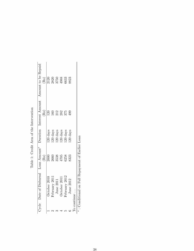
Tab
le1:
Cre
dit
Arm
ofth
eIn
terv
enti
on
Cycl
eD
ate
ofD
isb
urs
alL
oan
Am
ount∗
Du
rati
onIn
tere
stA
mou
nt
Am
ount
tob
eR
epaid
(Rs)
(Rs)
(Rs)
1O
ctob
er20
1020
0012
0d
ays
120
2120
2F
ebru
ary
2011
2660
120
day
s16
028
20
3Ju
ne
201
135
3812
0d
ays
212
3750
4O
ctob
er20
1147
0512
0d
ays
282
4988
5F
ebru
ary
2012
6258
120
day
s37
566
33
6Ju
ne
201
283
2312
0d
ays
499
8823
To
conti
nu
e...
∗:
Con
dit
ion
al
on
Fu
llR
epay
men
tof
Ear
lier
Loa
n
38
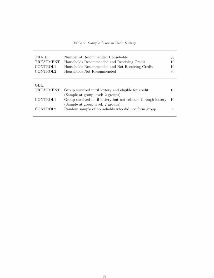
Table 2: Sample Sizes in Each Village
TRAIL: Number of Recommended Households 30TREATMENT Households Recommended and Receiving Credit 10CONTROL1 Households Recommended and Not Receiving Credit 10CONTROL2 Households Not Recommended 30
GBL:TREATMENT Group survived until lottery and eligible for credit 10
(Sample at group level: 2 groups)CONTROL1 Group survived until lottery but not selected through lottery 10
(Sample at group level: 2 groups)CONTROL2 Random sample of households who did not form group 30
39
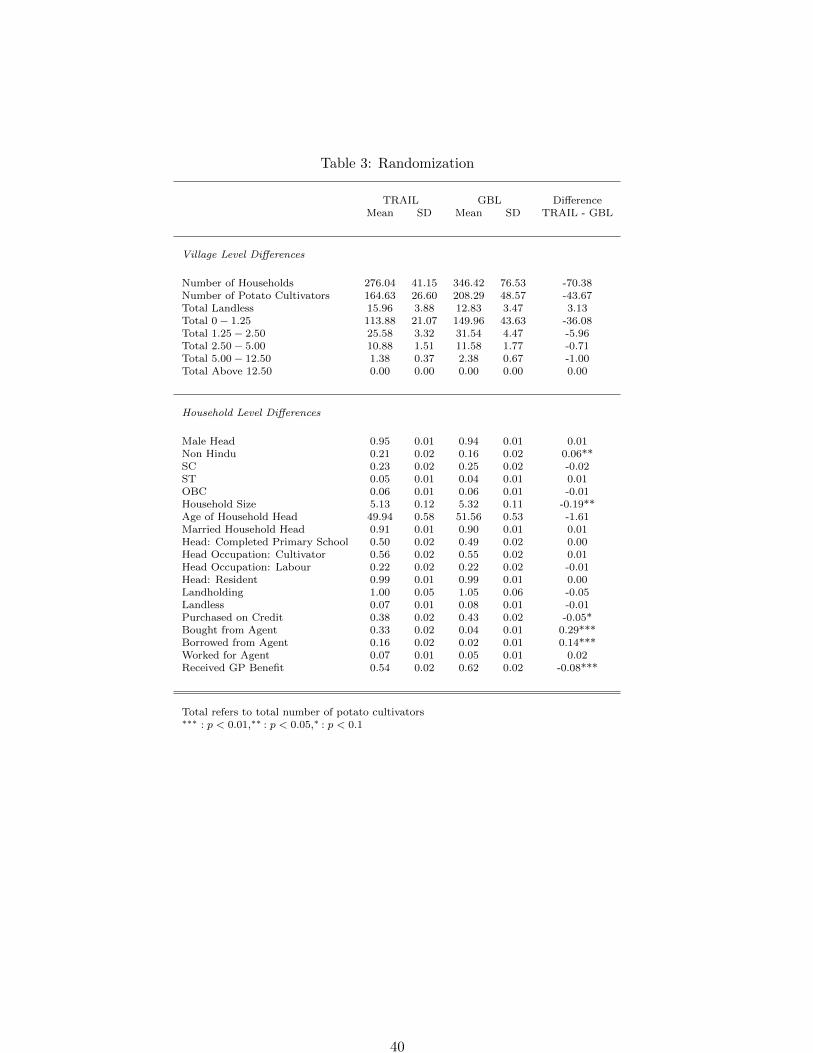
Table 3: Randomization
TRAIL GBL DifferenceMean SD Mean SD TRAIL - GBL
Village Level Differences
Number of Households 276.04 41.15 346.42 76.53 -70.38Number of Potato Cultivators 164.63 26.60 208.29 48.57 -43.67Total Landless 15.96 3.88 12.83 3.47 3.13Total 0− 1.25 113.88 21.07 149.96 43.63 -36.08Total 1.25− 2.50 25.58 3.32 31.54 4.47 -5.96Total 2.50− 5.00 10.88 1.51 11.58 1.77 -0.71Total 5.00− 12.50 1.38 0.37 2.38 0.67 -1.00Total Above 12.50 0.00 0.00 0.00 0.00 0.00
Household Level Differences
Male Head 0.95 0.01 0.94 0.01 0.01Non Hindu 0.21 0.02 0.16 0.02 0.06**SC 0.23 0.02 0.25 0.02 -0.02ST 0.05 0.01 0.04 0.01 0.01OBC 0.06 0.01 0.06 0.01 -0.01Household Size 5.13 0.12 5.32 0.11 -0.19**Age of Household Head 49.94 0.58 51.56 0.53 -1.61Married Household Head 0.91 0.01 0.90 0.01 0.01Head: Completed Primary School 0.50 0.02 0.49 0.02 0.00Head Occupation: Cultivator 0.56 0.02 0.55 0.02 0.01Head Occupation: Labour 0.22 0.02 0.22 0.02 -0.01Head: Resident 0.99 0.01 0.99 0.01 0.00Landholding 1.00 0.05 1.05 0.06 -0.05Landless 0.07 0.01 0.08 0.01 -0.01Purchased on Credit 0.38 0.02 0.43 0.02 -0.05*Bought from Agent 0.33 0.02 0.04 0.01 0.29***Borrowed from Agent 0.16 0.02 0.02 0.01 0.14***Worked for Agent 0.07 0.01 0.05 0.01 0.02Received GP Benefit 0.54 0.02 0.62 0.02 -0.08***
Total refers to total number of potato cultivators∗∗∗ : p < 0.01,∗∗ : p < 0.05,∗ : p < 0.1
40
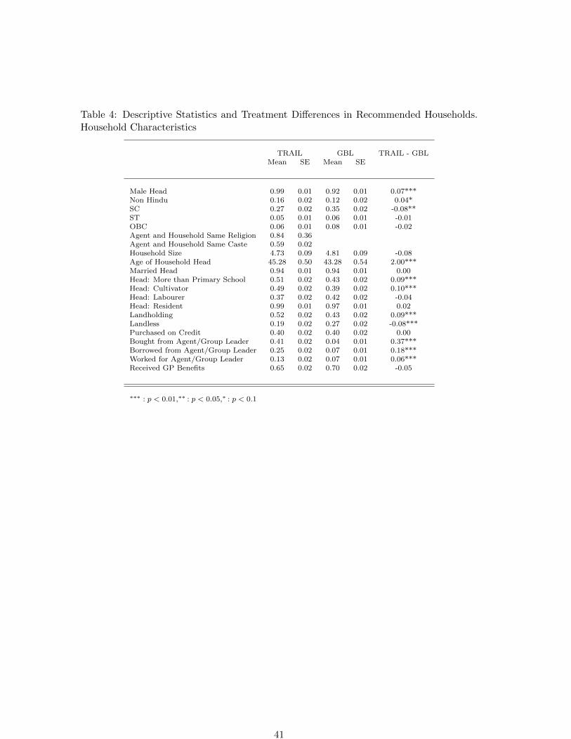
Table 4: Descriptive Statistics and Treatment Differences in Recommended Households.Household Characteristics
TRAIL GBL TRAIL - GBLMean SE Mean SE
Male Head 0.99 0.01 0.92 0.01 0.07***Non Hindu 0.16 0.02 0.12 0.02 0.04*SC 0.27 0.02 0.35 0.02 -0.08**ST 0.05 0.01 0.06 0.01 -0.01OBC 0.06 0.01 0.08 0.01 -0.02Agent and Household Same Religion 0.84 0.36Agent and Household Same Caste 0.59 0.02Household Size 4.73 0.09 4.81 0.09 -0.08Age of Household Head 45.28 0.50 43.28 0.54 2.00***Married Head 0.94 0.01 0.94 0.01 0.00Head: More than Primary School 0.51 0.02 0.43 0.02 0.09***Head: Cultivator 0.49 0.02 0.39 0.02 0.10***Head: Labourer 0.37 0.02 0.42 0.02 -0.04Head: Resident 0.99 0.01 0.97 0.01 0.02Landholding 0.52 0.02 0.43 0.02 0.09***Landless 0.19 0.02 0.27 0.02 -0.08***Purchased on Credit 0.40 0.02 0.40 0.02 0.00Bought from Agent/Group Leader 0.41 0.02 0.04 0.01 0.37***Borrowed from Agent/Group Leader 0.25 0.02 0.07 0.01 0.18***Worked for Agent/Group Leader 0.13 0.02 0.07 0.01 0.06***Received GP Benefits 0.65 0.02 0.70 0.02 -0.05
∗∗∗ : p < 0.01,∗∗ : p < 0.05,∗ : p < 0.1
41
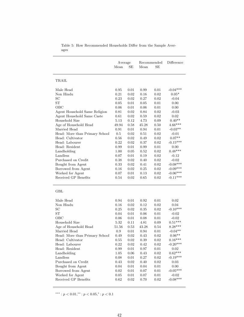
Table 5: How Recommended Households Differ from the Sample Aver-ages
Average Recommended DifferenceMean SE Mean SE
TRAIL
Male Head 0.95 0.01 0.99 0.01 -0.04***Non Hindu 0.21 0.02 0.16 0.02 0.05*SC 0.23 0.02 0.27 0.02 -0.04ST 0.05 0.01 0.05 0.01 0.00OBC 0.06 0.01 0.06 0.01 0.00Agent Household Same Religion 0.81 0.02 0.84 0.02 -0.03Agent Household Same Caste 0.61 0.02 0.59 0.02 0.02Household Size 5.13 0.12 4.73 0.09 0.40**Age of Household Head 49.94 0.58 45.28 0.50 4.66***Married Head 0.91 0.01 0.94 0.01 -0.03**Head: More than Primary School 0.5 0.02 0.51 0.02 -0.01Head: Cultivator 0.56 0.02 0.49 0.02 0.07**Head: Labourer 0.22 0.02 0.37 0.02 -0.15***Head: Resident 0.99 0.01 0.99 0.01 0.00Landholding 1.00 0.05 0.52 0.02 0.48***Landless 0.07 0.01 0.19 0.02 -0.12Purchased on Credit 0.38 0.02 0.40 0.02 -0.02Bought from Agent 0.33 0.02 0.41 0.02 -0.08***Borrowed from Agent 0.16 0.02 0.25 0.02 -0.09***Worked for Agent 0.07 0.01 0.13 0.02 -0.06***Received GP Benefits 0.54 0.02 0.65 0.02 -0.11***
GBL
Male Head 0.94 0.01 0.92 0.01 0.02Non Hindu 0.16 0.02 0.12 0.02 0.04SC 0.25 0.02 0.35 0.02 -0.10***ST 0.04 0.01 0.06 0.01 -0.02OBC 0.06 0.01 0.08 0.01 -0.02Household Size 5.32 0.11 4.81 0.09 0.51***Age of Household Head 51.56 0.53 43.28 0.54 8.28***Married Head 0.9 0.01 0.94 0.01 -0.04**Head: More than Primary School 0.49 0.02 0.43 0.02 0.06**Head: Cultivator 0.55 0.02 0.39 0.02 0.16***Head: Labourer 0.22 0.02 0.42 0.02 -0.20***Head: Resident 0.99 0.01 0.97 0.01 0.02Landholding 1.05 0.06 0.43 0.02 0.62***Landless 0.08 0.01 0.27 0.02 -0.19***Purchased on Credit 0.43 0.02 0.40 0.02 0.03Bought from Agent 0.04 0.01 0.04 0.01 0.00Borrowed from Agent 0.02 0.01 0.07 0.01 -0.05***Worked for Agent 0.05 0.01 0.07 0.01 -0.02Received GP Benefits 0.62 0.02 0.70 0.02 -0.08***
∗∗∗ : p < 0.01,∗∗ : p < 0.05,∗ : p < 0.1
42
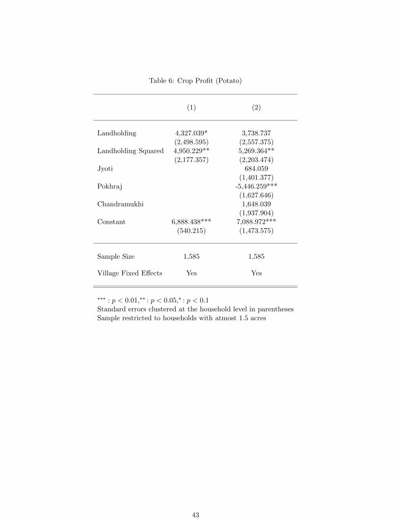
Table 6: Crop Profit (Potato)
(1) (2)
Landholding 4,327.039* 3,738.737(2,498.595) (2,557.375)
Landholding Squared 4,950.229** 5,269.364**(2,177.357) (2,203.474)
Jyoti 684.059(1,401.377)
Pokhraj -5,446.259***(1,627.646)
Chandramukhi 1,648.039(1,937.904)
Constant 6,888.438*** 7,088.972***(540.215) (1,473.575)
Sample Size 1,585 1,585
Village Fixed Effects Yes Yes
∗∗∗ : p < 0.01,∗∗ : p < 0.05,∗ : p < 0.1Standard errors clustered at the household level in parenthesesSample restricted to households with atmost 1.5 acres
43
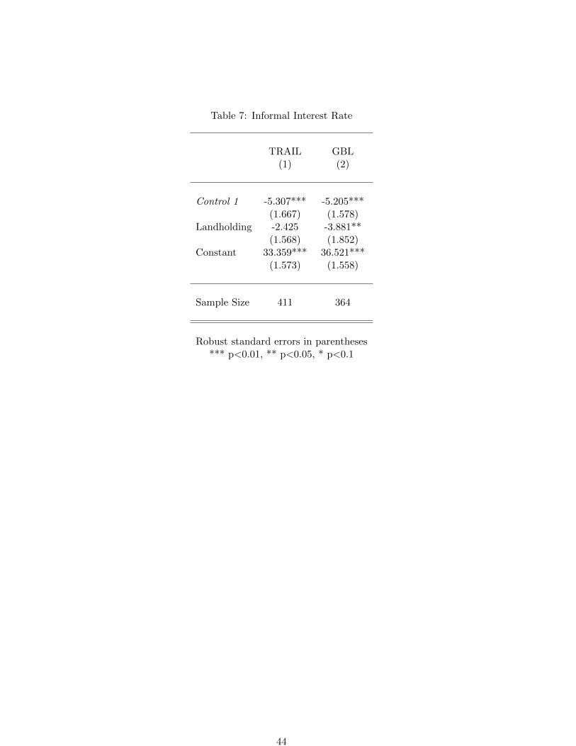
Table 7: Informal Interest Rate
TRAIL GBL(1) (2)
Control 1 -5.307*** -5.205***(1.667) (1.578)
Landholding -2.425 -3.881**(1.568) (1.852)
Constant 33.359*** 36.521***(1.573) (1.558)
Sample Size 411 364
Robust standard errors in parentheses*** p<0.01, ** p<0.05, * p<0.1
44
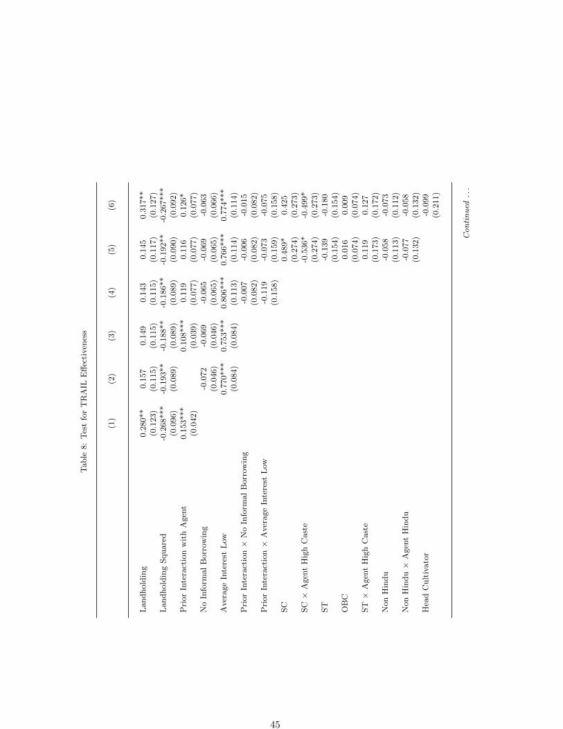
Table
8:
Tes
tfo
rT
RA
ILE
ffec
tiven
ess
(1)
(2)
(3)
(4)
(5)
(6)
Landhold
ing
0.2
80**
0.1
57
0.1
49
0.1
43
0.1
45
0.3
17**
(0.1
23)
(0.1
15)
(0.1
15)
(0.1
15)
(0.1
17)
(0.1
27)
Landhold
ing
Square
d-0
.268***
-0.1
93**
-0.1
88**
-0.1
86**
-0.1
92**
-0.2
67***
(0.0
96)
(0.0
89)
(0.0
89)
(0.0
89)
(0.0
90)
(0.0
92)
Pri
or
Inte
ract
ion
wit
hA
gen
t0.1
53***
0.1
08***
0.1
19
0.1
16
0.1
26*
(0.0
42)
(0.0
39)
(0.0
77)
(0.0
77)
(0.0
77)
No
Info
rmal
Borr
owin
g-0
.072
-0.0
69
-0.0
65
-0.0
69
-0.0
63
(0.0
46)
(0.0
46)
(0.0
65)
(0.0
65)
(0.0
66)
Aver
age
Inte
rest
Low
0.7
70***
0.7
53***
0.8
06***
0.7
66***
0.7
74***
(0.0
84)
(0.0
84)
(0.1
13)
(0.1
14)
(0.1
14)
Pri
or
Inte
ract
ion×
No
Info
rmal
Borr
owin
g-0
.007
-0.0
06
-0.0
15
(0.0
82)
(0.0
82)
(0.0
82)
Pri
or
Inte
ract
ion×
Aver
age
Inte
rest
Low
-0.1
19
-0.0
73
-0.0
75
(0.1
58)
(0.1
59)
(0.1
58)
SC
0.4
89*
0.4
25
(0.2
74)
(0.2
73)
SC×
Agen
tH
igh
Cast
e-0
.536*
-0.4
99*
(0.2
74)
(0.2
73)
ST
-0.1
39
-0.1
80
(0.1
54)
(0.1
54)
OB
C0.0
16
0.0
09
(0.0
74)
(0.0
74)
ST×
Agen
tH
igh
Cast
e0.1
19
0.1
27
(0.1
73)
(0.1
72)
Non
Hin
du
-0.0
58
-0.0
73
(0.1
13)
(0.1
12)
Non
Hin
du×
Agen
tH
indu
-0.0
77
-0.0
58
(0.1
32)
(0.1
32)
Hea
dC
ult
ivato
r-0
.099
(0.2
11)
Co
nti
nu
ed...
45
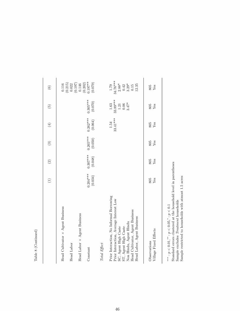
Table
8(C
onti
nued
)
(1)
(2)
(3)
(4)
(5)
(6)
Hea
dC
ult
ivato
r×
Agen
tB
usi
nes
s0.1
16
(0.2
15)
Hea
dL
ab
or
0.0
22
(0.1
97)
Hea
dL
ab
or×
Agen
tB
usi
nes
s0.1
46
(0.2
02)
Const
ant
0.2
04***
0.3
07***
0.2
65***
0.2
62***
0.3
05***
0.1
97**
(0.0
34)
(0.0
48)
(0.0
50)
(0.0
64)
(0.0
70)
(0.0
79)
To
tal
Eff
ect
Pri
or
Inte
ract
ion,
No
Info
rmal
Borr
owin
g1.5
41.6
31.7
9P
rior
Inte
ract
ion,
Aver
age
Inte
rest
Low
33.4
1***
33.8
9***
34.7
6***
SC
,A
gen
tH
igh
Cast
e1.2
12.8
8*
ST
,A
gen
tH
igh
Cast
e0.0
60.4
2N
on
Hin
du,
Agen
tH
indu
3.4
7*
3.2
9*
Hea
dC
ult
ivato
r,A
gen
tB
usi
nes
s0.1
5H
ead
Lab
or,
Agen
tB
usi
nes
s12.3
5
Obse
rvati
ons
805
805
805
805
805
805
Villa
ge
Fix
edE
ffec
tsY
esY
esY
esY
esY
esY
es
∗∗∗
:p<
0.0
1,∗∗
:p<
0.0
5,∗
:p<
0.1
Sta
ndard
erro
rscl
ust
ered
at
the
house
hold
level
inpare
nth
eses
Sam
ple
excl
udes
Tre
atm
ent
house
hold
sSam
ple
rest
rict
edto
house
hold
sw
ith
atm
ost
1.5
acr
es
46
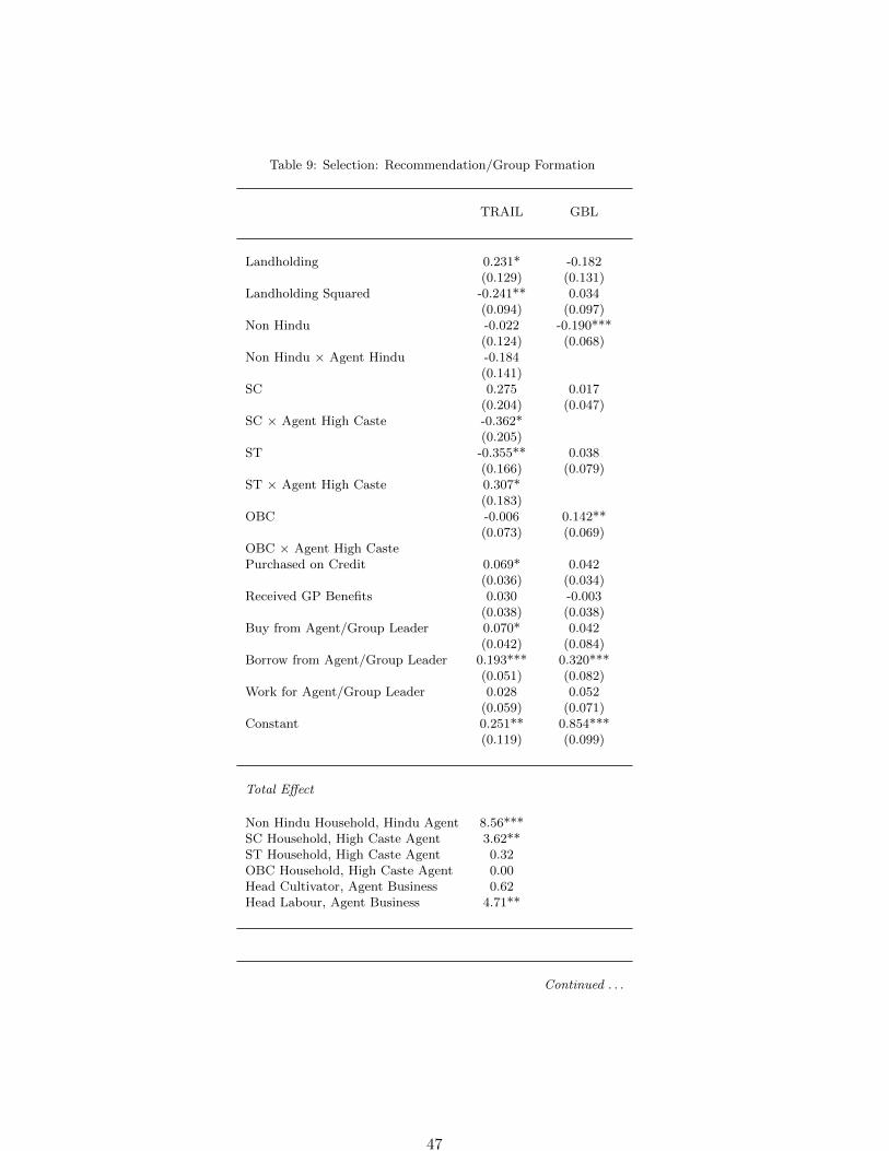
Table 9: Selection: Recommendation/Group Formation
TRAIL GBL
Landholding 0.231* -0.182(0.129) (0.131)
Landholding Squared -0.241** 0.034(0.094) (0.097)
Non Hindu -0.022 -0.190***(0.124) (0.068)
Non Hindu × Agent Hindu -0.184(0.141)
SC 0.275 0.017(0.204) (0.047)
SC × Agent High Caste -0.362*(0.205)
ST -0.355** 0.038(0.166) (0.079)
ST × Agent High Caste 0.307*(0.183)
OBC -0.006 0.142**(0.073) (0.069)
OBC × Agent High CastePurchased on Credit 0.069* 0.042
(0.036) (0.034)Received GP Benefits 0.030 -0.003
(0.038) (0.038)Buy from Agent/Group Leader 0.070* 0.042
(0.042) (0.084)Borrow from Agent/Group Leader 0.193*** 0.320***
(0.051) (0.082)Work for Agent/Group Leader 0.028 0.052
(0.059) (0.071)Constant 0.251** 0.854***
(0.119) (0.099)
Total Effect
Non Hindu Household, Hindu Agent 8.56***SC Household, High Caste Agent 3.62**ST Household, High Caste Agent 0.32OBC Household, High Caste Agent 0.00Head Cultivator, Agent Business 0.62Head Labour, Agent Business 4.71**
Continued . . .
47
Table 9 (Continued)
TRAIL GBL
Sample Size 1,031 1,038Number of Villages 24 24Village Fixed Effects Yes Yes
Linear Probability EstimatesRobust Standard errors in parenthesesSample restricted to households with at most 1.5 acres∗∗∗ : p < 0.01,∗∗ : p < 0.05,∗ : p < 0.1Regressions also control for age, gender, educational attainment,
and primary occupation of the household headand interactions with the primary occupation of the agent,and household size
48
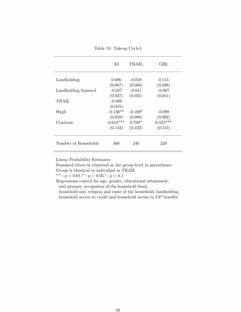
Table 10: Takeup Cycle1
All TRAIL GBL
Landholding 0.006 -0.058 0.113(0.067) (0.088) (0.098)
Landholding Squared -0.027 -0.011 -0.067(0.027) (0.031) (0.051)
TRAIL -0.009(0.055)
Hugli -0.136** -0.169* -0.098(0.058) (0.086) (0.092)
Constant 0.644*** 0.794* 0.555***(0.133) (0.423) (0.155)
Number of Households 460 240 220
Linear Probability EstimatesStandard errors in clustered at the group level in parenthesesGroup is identical to individual in TRAIL∗∗∗ : p < 0.01,∗∗ : p < 0.05,∗ : p < 0.1Regressions control for age, gender, educational attainment,
and primary occupation of the household head,household size, religion and caste of the household, landholding,household access to credit and household access to GP benefits
49
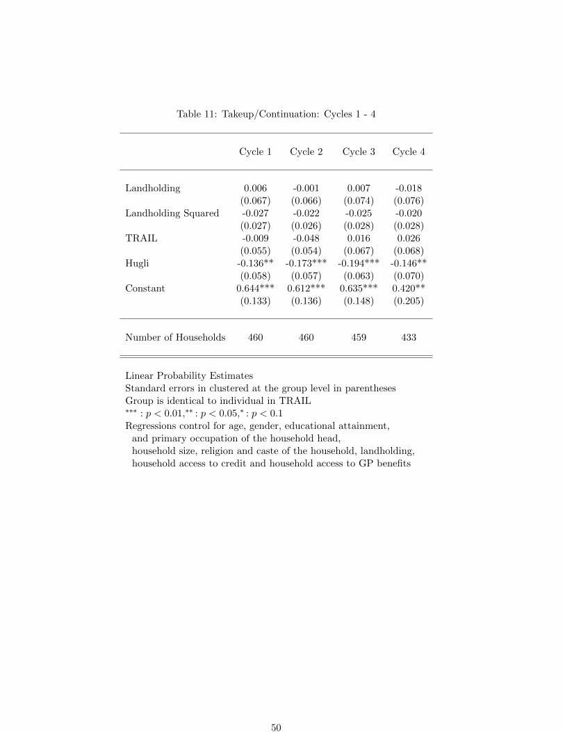
Table 11: Takeup/Continuation: Cycles 1 - 4
Cycle 1 Cycle 2 Cycle 3 Cycle 4
Landholding 0.006 -0.001 0.007 -0.018(0.067) (0.066) (0.074) (0.076)
Landholding Squared -0.027 -0.022 -0.025 -0.020(0.027) (0.026) (0.028) (0.028)
TRAIL -0.009 -0.048 0.016 0.026(0.055) (0.054) (0.067) (0.068)
Hugli -0.136** -0.173*** -0.194*** -0.146**(0.058) (0.057) (0.063) (0.070)
Constant 0.644*** 0.612*** 0.635*** 0.420**(0.133) (0.136) (0.148) (0.205)
Number of Households 460 460 459 433
Linear Probability EstimatesStandard errors in clustered at the group level in parenthesesGroup is identical to individual in TRAIL∗∗∗ : p < 0.01,∗∗ : p < 0.05,∗ : p < 0.1Regressions control for age, gender, educational attainment,
and primary occupation of the household head,household size, religion and caste of the household, landholding,household access to credit and household access to GP benefits
50
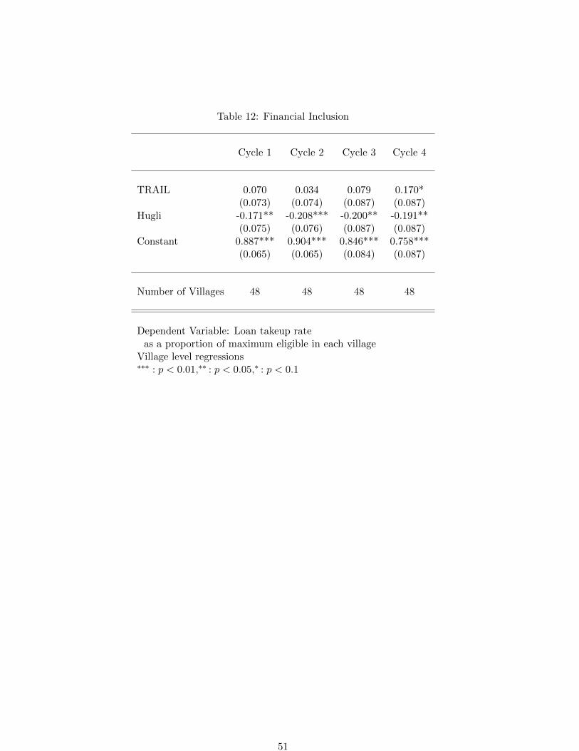
Table 12: Financial Inclusion
Cycle 1 Cycle 2 Cycle 3 Cycle 4
TRAIL 0.070 0.034 0.079 0.170*(0.073) (0.074) (0.087) (0.087)
Hugli -0.171** -0.208*** -0.200** -0.191**(0.075) (0.076) (0.087) (0.087)
Constant 0.887*** 0.904*** 0.846*** 0.758***(0.065) (0.065) (0.084) (0.087)
Number of Villages 48 48 48 48
Dependent Variable: Loan takeup rateas a proportion of maximum eligible in each village
Village level regressions∗∗∗ : p < 0.01,∗∗ : p < 0.05,∗ : p < 0.1
51
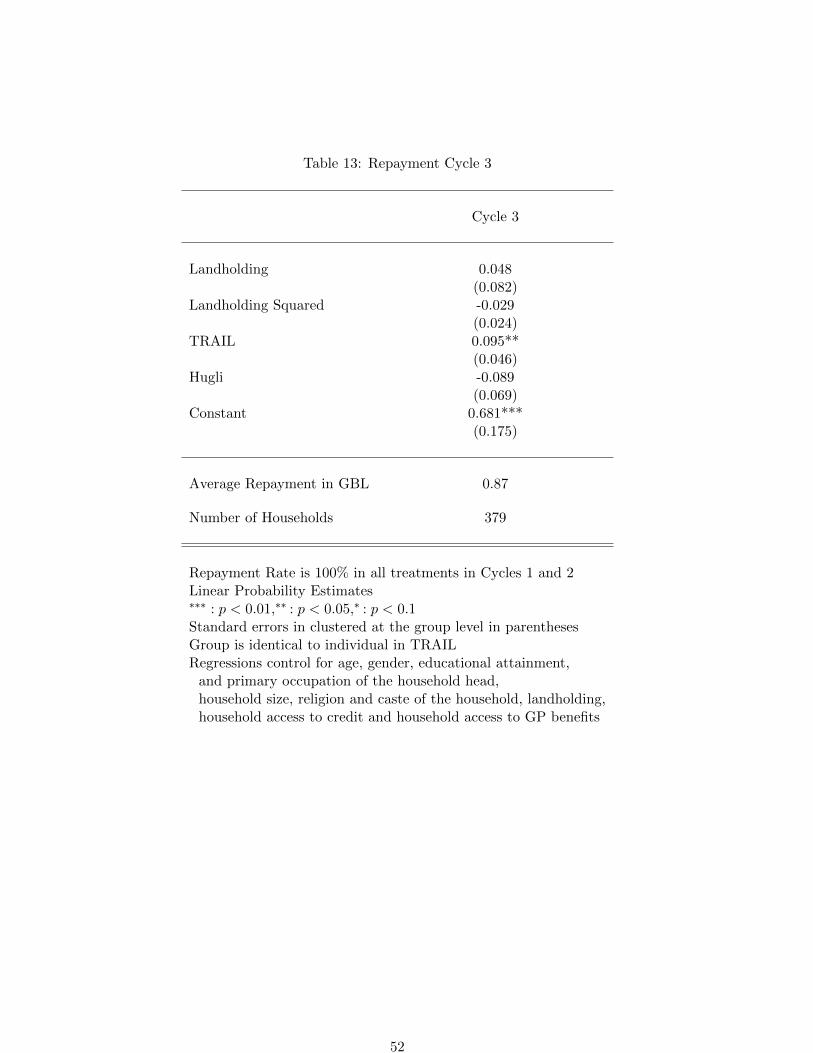
Table 13: Repayment Cycle 3
Cycle 3
Landholding 0.048(0.082)
Landholding Squared -0.029(0.024)
TRAIL 0.095**(0.046)
Hugli -0.089(0.069)
Constant 0.681***(0.175)
Average Repayment in GBL 0.87
Number of Households 379
Repayment Rate is 100% in all treatments in Cycles 1 and 2Linear Probability Estimates∗∗∗ : p < 0.01,∗∗ : p < 0.05,∗ : p < 0.1Standard errors in clustered at the group level in parenthesesGroup is identical to individual in TRAILRegressions control for age, gender, educational attainment,
and primary occupation of the household head,household size, religion and caste of the household, landholding,household access to credit and household access to GP benefits
52
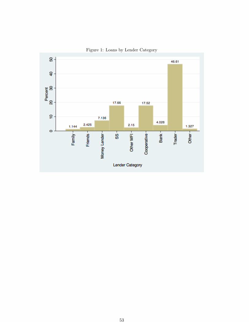
Figure 1: Loans by Lender Category
53
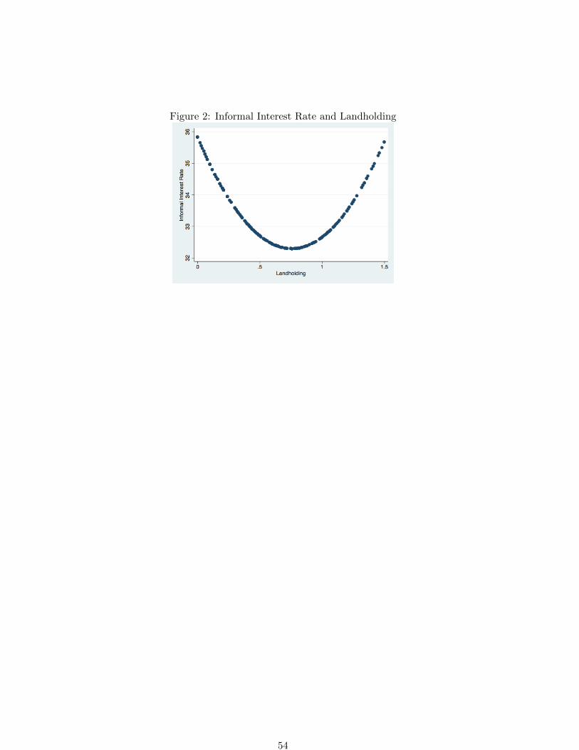
Figure 2: Informal Interest Rate and Landholding
54
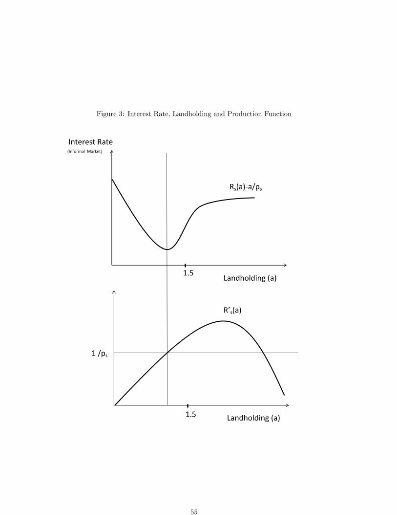
Figure 3: Interest Rate, Landholding and Production Function
Interest Rate
(Informal Market)
R’s(a)
Landholding (a) 1.5
Rs(a)-a/ps
1.5
1 /ps
Landholding (a)
55
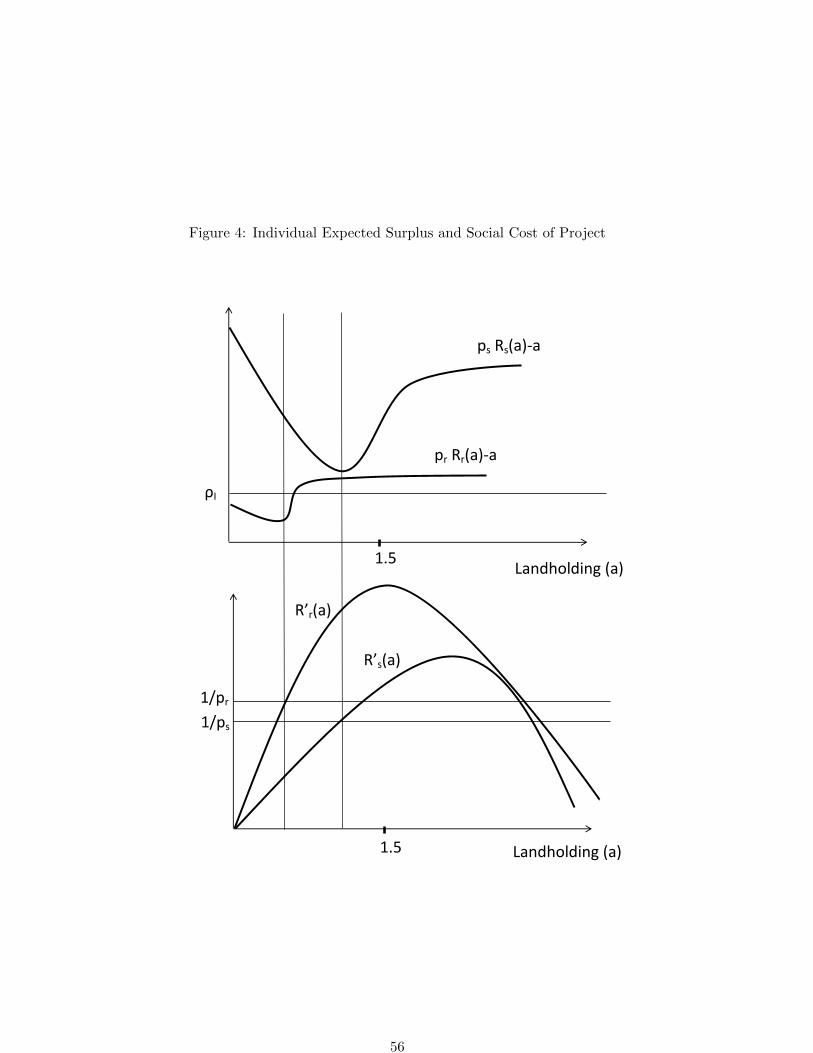
Figure 4: Individual Expected Surplus and Social Cost of Project
ρI
R’s(a)
R’r(a)
1/ps
1/pr
Landholding (a) 1.5
ps Rs(a)-a
1.5
pr Rr(a)-a
Landholding (a)
56
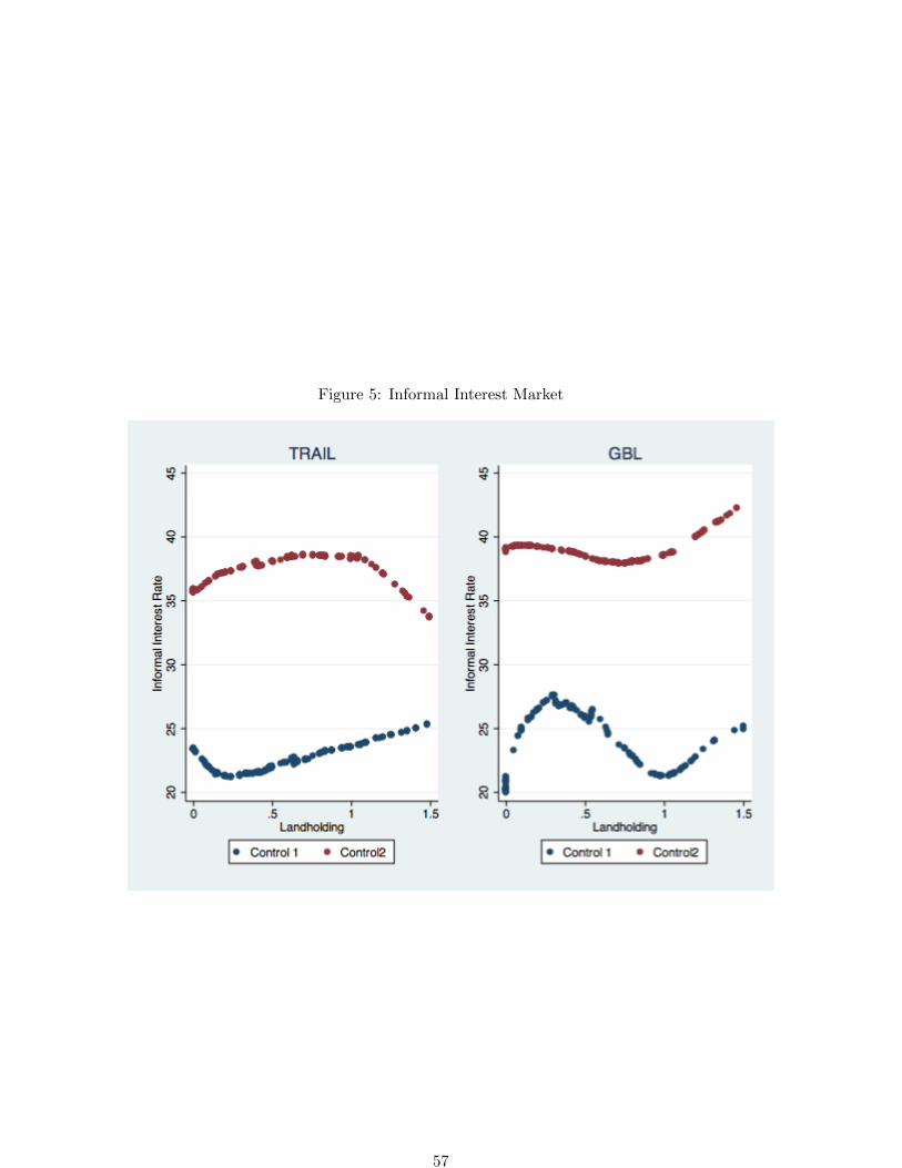
Figure 5: Informal Interest Market
57
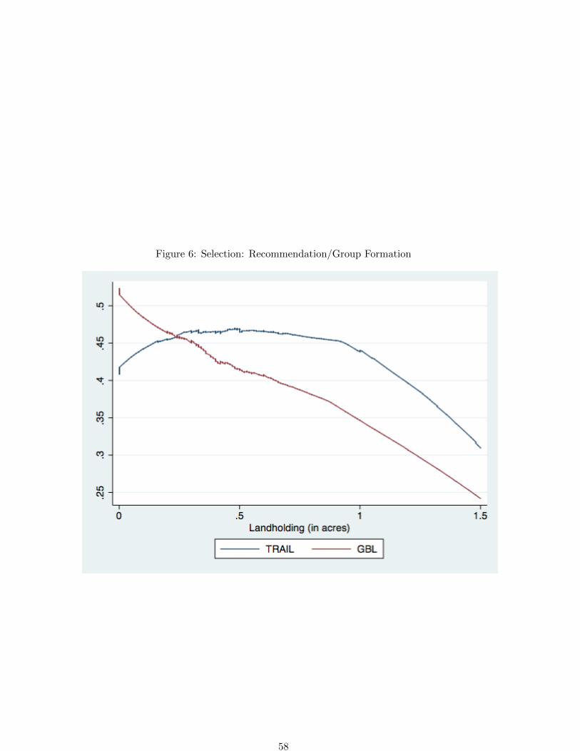
Figure 6: Selection: Recommendation/Group Formation
58
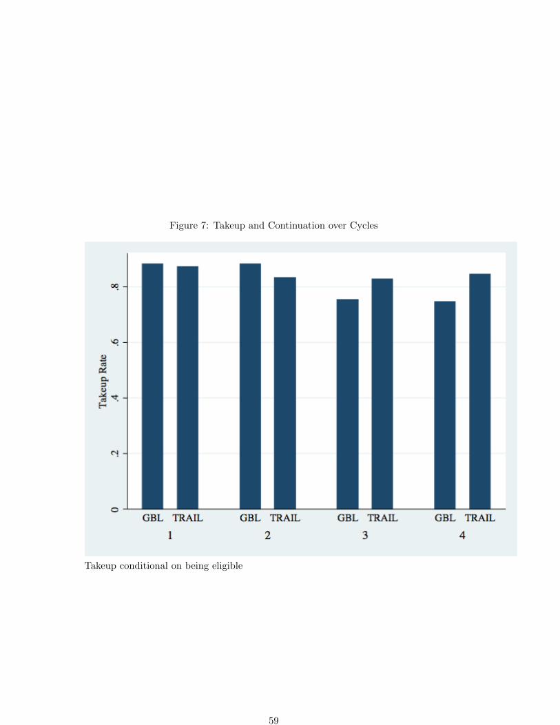
Figure 7: Takeup and Continuation over Cycles
Takeup conditional on being eligible
59
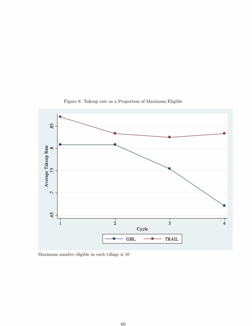
Figure 8: Takeup rate as a Proportion of Maximum Eligible
Maximum number eligible in each village is 10
60
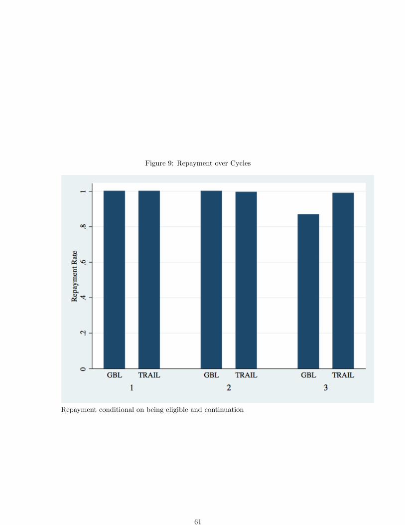
Figure 9: Repayment over Cycles
Repayment conditional on being eligible and continuation
61