Interleaved Text/Image Deep Miningon a Large-Scale Radiology Database

Hoo-Chang Shin Le Lu Lauren Kim Ari Seff Jianhua Yao Ronald M. Summers

Imaging Biomarkers and Computer-Aided Diagnosis LaboratoryRadiology and Imaging Sciences

National Institutes of Health Clinical CenterBethesda, MD 20892-1182

{hoochang.shin, le.lu, lauren.kim2, ari.seff, rms}@nih.gov, jyao@cc.nih.gov

Abstract

Despite tremendous progress in computer vision, effec-tive learning on very large-scale (> 100K patients) medi-cal image databases has been vastly hindered. We presentan interleaved text/image deep learning system to extractand mine the semantic interactions of radiology images andreports from a national research hospital’s picture archiv-ing and communication system. Instead of using full 3Dmedical volumes, we focus on a collection of representa-tive ~216K 2D key images/slices (selected by clinicians fordiagnostic reference) with text-driven scalar and vector la-bels. Our system interleaves between unsupervised learn-ing (e.g., latent Dirichlet allocation, recurrent neural netlanguage models) on document- and sentence-level texts togenerate semantic labels and supervised learning via deepconvolutional neural networks (CNNs) to map from imagesto label spaces. Disease-related key words can be predictedfor radiology images in a retrieval manner. We have demon-strated promising quantitative and qualitative results. Thelarge-scale datasets of extracted key images and their cat-egorization, embedded vector labels and sentence descrip-tions can be harnessed to alleviate the deep learning “data-hungry” obstacle in the medical domain.

1. Introduction

The ImageNet Large Scale Visual Recognition Chal-lenge [8] provides more than one million labeled imagesfrom 1,000 object categories. The accessibility of a hugeamount of well-annotated image data in computer visionrekindles deep convolutional neural networks (CNNs) [24,41, 45] as a premier learning tool to solve the visual objectclass recognition tasks. Deep CNNs can perform signifi-cantly better than traditional shallow learning methods, but

total number of # words in documents # image modalities# documents ∼780k mean 131.13 CT ∼169k# images ∼216k std 95.72 MR ∼46k# words ∼1 billion max 1502 PET 67# vocabulary ∼29k min 2 others 34

Table 1. Some statistics of the dataset. “Others” include CR(Computed Radiography), RF (Radio Fluoroscopy), and US (Ul-trasound).

right 937k images 312k contrast 260k unremarkable 195kleft 870k seen 299k axial 253k lower 195k

impression 421k mass 296k lung 243k upper 192kevidence 352k normal 278k bone 219k lesion 180kfindings 340k small 275k chest 208k lobe 174k

CT 312k noted 263k MRI 204k pleural 172k

Table 2. Examples of the most frequently occurring words in theradiology report documents.

usually requires much more training data [24, 38]. In themedical domain, however, there are no similar large-scalelabeled image datasets available. On the other hand, gigan-tic collections of radiology images and reports are storedin many modern hospitals’ picture archiving and commu-nication system (PACS). The invaluable semantic diagnos-tic knowledge inhabiting the mapping between hundreds ofthousands of clinician-created high quality text reports andlinked image volumes remains largely unexplored. One ofour primary goals is to extract and associate radiology im-ages with clinically semantic scalar and vector labels viainterleaved text/image data mining and deep learning on alarge-scale PACS database (~780K imaging examinations).To the best of our knowledge, this is the first reported workof “Deep Mining into PACS” at a very large scale.

Building the ImageNet database was mainly a manualprocess [8]: harvesting images returned from Google im-age search engine (according to the WordNet ontology hi-

1

erarchy) and pruning falsely tagged images using crowd-sourcing such as Amazon Mechanical Turk (AMT). Thisdoes not meet our data collection and labeling needs due tothe demanding difficulties of medical annotation tasks andthe data privacy reasons. Thus we propose to mine imagecategorization labels from hierarchical, Bayesian documentclustering method, e.g., generative latent Dirichlet alloca-tion (LDA) topic modeling [6], using all available radiol-ogy text reports in PACS. The Radiology reports are textdocuments describing patient history, symptoms, image ob-servations and impressions written by board-certified radi-ologists. However, the reports do not contain specific im-age labels to be trained my a machine learning algorithm.We find that LDA-generated image categorization labelsare valid, demonstrating good semantic coherence amongclinician observers [22, 11], and can be effectively learnedusing deep CNNs with image inputs alone [24, 41]. Ourdeep CNN models on medical image modalities (mostly CT,MRI) are initialized with the model parameters pre-trainedfrom ImageNet [8] using Caffe [19] framework. Kulkarni etal. [25] have spearheaded the efforts of learning the seman-tic connections between image contents and the sentencesdescribing them (i.e., captions). Detecting objects of inter-est, attributes and prepositions and applying contextual reg-ularization with a conditional random field (CRF) is a feasi-ble approach [25] because many useful tools are available incomputer vision. There has not yet been much comparabledevelopment on large-scale medical imaging understanding.

Our work has been inspired by the works building verylarge-scale image databases [8, 38] and the works estab-lishing semantic connections of texts and images [25]. Weobserve good semantic coherence between labels obtainedby hierarchical document topic models [6] and clinician’sassessment. Based on this, both unsupervised (recurrentneural net language models [30, 32]) and supervised deepCNNs with categorization and regression losses are usedfor annotating large collection of radiology images. Thefact that deep learning requires no hand-crafted image fea-tures is very desirable since significant adaption would beneeded to apply conventional image features, e.g., HOG,SIFT for medical image learning. The large-scale datasetsof extracted key images and their categorization, vector la-bels, describing sentences can be harnessed to alleviate deeplearning’s “data-hungry” challenge in the medical domain1.

1.1. Related Work

The ImageCLEF medical image annotation tasks of2005-2007 have 9,000 training and 1,000 testing 2D images(converted as 32×32 pixel thumbnails in [9]) with 57 labels.Local image descriptors and intensity histograms are used

1We are currently working on the institutional review board ap-proval to share our extracted data (not original full radiology reports).We make our code and trained deep text/image models available inhttps://github.com/rsummers11/CADLab.

in a bag-of-features approach in that work for this scenerecognition-like problem. Unsupervised latent Dirichlet al-location based matching from lung disease words (e.g., fi-brosis, emphysema) in radiology reports to 2D image blocksfrom axial CT chest scans (of 24 patients) is studied in [7].This work is motivated by generative models of combiningwords and images [2, 5] under a very limited word/imagevocabulary.

The most related works are [42, 11] which first mapwords into vector space using recurrent neural networks andthen project images into the label-associated word-vectorembeddings by minimizing the L2 ([42]) or hinge ranklosses ([11]) between the visual and label manifolds. Thelanguage model is trained on the texts of Wikipedia andtested on label-associated images from the CIFAR [23, 42]and ImageNet [8, 11] datsets. In comparison, our work ison a large, unlabeled medical dataset of associated imagesand text, where the text-derived labels are computed andverified with human intervention. Image-to-language cor-respondence was learned from ImageNet dataset and rea-sonably high quality image description datasets (Pascal1K[36], Flickr8K [16], Flickr30K [47]) in [20], where suchcaption datasets are not available in the medical domain.Graphical models have been employed to predict image at-tributes ([27, 39]), or to describe images ([25]) using man-ually annotated datasets ([36, 26]). Automatic label miningon large, unlabeled datasets is presented in [35, 18], how-ever the variety of the label-space is limited (image text an-notations). We analyze/mine the medical image semanticson both document and sentence levels, and deep CNNs areadapted to learn them from image contents [18, 41].

2. Data

To gain the most comprehensive understanding of diag-nostic semantics, we use all available radiology reports ofaround ~780K imaging examinations, stored in the PACSof National Institutes of Health Clinical Center since theyear 2000. Around 216K key 2D image slices (instead ofall 3D image volumes) are studied here. Within 3D pa-tient scans, most of the imaging information represented isnormal anatomy, i.e, not the focus of the radiology reports.These “key images” were referenced (see Figure 1) by ra-diologists manually during radiology report writing, to pro-vide a visual reference to pathologies or other notable find-ings. Therefore 2D key images are more correlated with thediagnostic semantics in the reports than the whole 3D scans,but not all reports have referenced key images (215, 786 im-ages from 61, 845 unique patients). Table 1 provides ex-tracted database statistics, and Table 2 shows examples ofthe most frequently occurring words in radiology reports.Leveraging our deep learning models exploited in this pa-per will make it possible to automatically select key imagesfrom 3D patient scans to avoid mis-referencing.

0001#REPORT# :# REASON#FOR#EXAM# (Entered#by# ordering# clinician# into#CRIS):# hx# of# head# and#neck#cancer.#needs#scan#CT#of#the#nasopharynx.#HISTORY:#Head#and#neck#cancer.#TECHNIQUE:# ConLguous# 2.5# mm# axial# images# of# the# nasopharynx# were# performed# without# IV#contrast.#COMPARISON:#xx/xx/xxxx.#FINDINGS:# No# soV# Lssue# masses# are# seen# within# the# soV# Lssues# of# the# neck.# The# paroLd# and#submandibular# glands# are# predominantly# faWyXreplaced.# SoV# Lssues# of# the# Naso,# oropharynx# are#unremarkable.#There#may#be#mild#fat#stranding#of#the#right#parapharyngeal#soV#Lssues#(series#1001,#image#32).#No#abnormal#masses#are#seen#at#that#site.#No#bulky#lymphadenopathy#is#seen.#There#is#a#fusiform#aneurysm#of#the#basilar#artery#as#previously#described.#It#appears#to#the#mildly#increased#in#size# and# currently#measures# 2.0# cm# in# transverse# dimensions# and# previously#measured# 1.8# cm.# It#measured#1.5#cm#in#transverse#dimensions#on#xx/xx/xxxx.#AtheroscleroLc#calcificaLons#are#also#seen#within# the#caroLd#arteries#bilaterally.#There# is#nearXcomplete#opacificaLon#of# the#maxillary# sinuses#bilaterally.# This# has# increased# predominantly# within# the# leV#maxillary# sinus# and#mildly# within# the#right# maxillary# sinus.# The# ethmoidal# air# cells# are# clear.# Sphenoidal# and# frontal# sinuses# are# clear.#DegeneraLve#changes#of#the#cervical#spine#are#noted.##IMPRESSIONS:#1.#No#soV#Lssue#masses#however,#mild# right#parapharyngeal# fat# stranding# is# seen# it#may# be# postoperaLve# or# post# radiaLon# in# nature.# 2.# Basilar# artery# aneurysm# that# has# gradually#increased# in#size#when#compared#to#prior#examinaLons.#3.#AtheroscleroLc#disease#of# the#coronary#arteries#bilaterally..##

0001#Report:#CHEST,#ABDOMEN,#PELVIS#CT:#MulLdetector#helical#(5#mm,#quad)#images#following,#and#abdomen# images# prior# to# vascular# contrast# infusion# (45# s# delay,# 2# cc/s,# 130# cc# Isovue)# obtained#without# apparent# complicaLon.#History:# renal# cell# pt# on#Medarex# protocol# here# for# end#of# course#evaluaLon.#CHEST:#MulLple#right,#and#at#least#one#leV#lung#masses#minimallyXmoderately#increasing#since#xx/xx/xxxx,#compaLble#with#metastases#despite#moderate#decrease#in#at#least#one#right#midXlung#mass#(e.g.#series#4# image#30).#Minimal#pretracheal# and# subcarinal# adenopathy# increasing.# Spine#osteophytes.#Enlargement#thyroid#on#right#side,#and#thyroid#heterogeneity#unchanged,#possibly#due#to#goiter.#No#evidence#of#pleural#or#pericardial#effusion,#axilla#or#leV#hilum#adenopathy.#ABDOMEN,#PELVIS:#Few#right#and#leV#liver#foci,#leV#periaorLc#and#leV#adrenal#fossa,#and#right#sacrum#mass# and# lyLc# lesion# (series# 3# image# 88X95)# increasing# minimally,# compaLble# with# metastases.#ScaWered# lumbar# vertebra# and# bilateral# ilium# foci# (e.g.# series# 3# image# 55,# 60,# 80,# 84X7,# 96)# foci#possibly#due#to#bone#metastases.#Uterine#fundus#focus#(series#3#image#95)#increasing#in#density#since#xx/xx/xxxx,# possibly# due# to# fibroid,# metastasis.# No# evidence# of# splenomegaly,# hydronephrosis,#gallbladder#calcificaLon,#or#bulky#mesenteric#adenopathy.#

Figure 1. Two examples of radiology reports and the referenced“key images” (providing a visual reference to pathologies or othernotable findings).

Finding and extracting key images from radiology re-ports is done by natural language processing (NLP), i.e,finding a sentence mentioning a referenced image. For ex-ample, “There may be mild fat stranding of the right para-pharyngeal soft tissues (series 1001, image 32)” is listedin Figure 1. The NLP steps [4] are sentence tokenization,word/number matching and stemming, and rule-based in-formation extraction (e.g., translating “image 1013-78” to“images 1013-1078”). A total of ~187K images can beretrieved and matched in this manner, whereas the rest of~28K key images are extracted according to their referenceaccession numbers in PACS. Our report-extracted key im-age database is the largest one ever reported and is highlyrepresentative of the huge collection of radiology diagnos-tic semantics over the last decade. Exploring effective deeplearning models on this database opens new ways to parseand understand large-scale radiology image informatics.

3. Document Topic Learning with LatentDirichlet Allocation

We propose to mine image categorization labels usingunsupervised document topic-modeling algorithm, e.g. la-tent Dirichlet allocation (LDA) [6], on the ~780K radiologytext reports in PACS. Unlike images from ImageNet [8, 38]which often have a dominant object appearing in the center,our key images are CT/MRI slices showing several coexist-ing organs/pathologies. There are high amounts of intrinsicambiguity in defining and assigning a semantic label set toimages, even for experienced clinicians. Our hypothesis isthat the large collection of sub-million radiology reports sta-tistically defines the categories meaningful for topic-mining(LDA) and visual learning (deep CNN).

LDA [6] was originally proposed to find latent topic

models for a collection of text documents (e.g., newspa-pers). There are some other popular methods for docu-ment topic modeling, such as Probabilistic Latent SemanticAnalysis (pLSA) [17] and Non-negative Matrix Factoriza-tion (NMF) [29]. We choose LDA for extracting latent topiclabels among radiology report documents because LDA isshown to be more flexible yet learns more coherent topicsover large sets of documents [43]. Furthermore, pLSA canbe regarded as a special case of LDA [13] and NMF as asemi-equivalent model of pLSA [12, 10].

LDA offers a hierarchy of extracted topics and the num-ber of topics can be chosen by evaluating each model’s per-plexity score (Equation 1), which is a common way to mea-sure how well a probabilistic model generalizes by evalu-ating the log-likelihood of the model on a held-out test set.For an unseen document set Dtest, the perplexity score isdefined as in Equation 1, where M is the number of doc-uments in the test set (unseen hold-out set of documents),wd the words in the unseen document d, Nd the number ofwords in document d, with Φ the topic matrix, and α thehyperparameter for topic distribution of the documents.

perplexity(Dtest) = exp

{−∑M

d=1 log p(wd|Φ, α)∑Md=1Nd

}(1)

A lower perplexity score generally implies a better fit of themodel for a given document set [6].

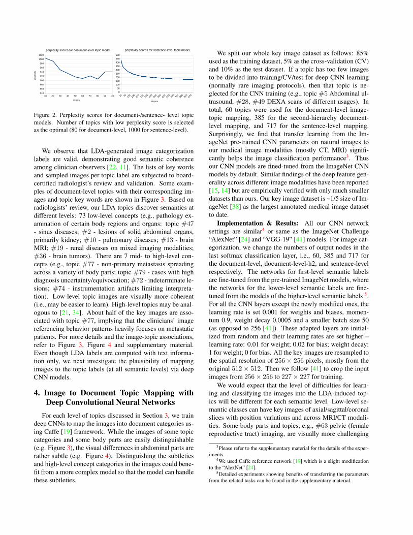
Based on the perplexity score evaluated on 80% of thetotal documents used for training and 20% used for testing,the number of topics chosen is 80 for the document-levelmodel using perplexity scores for model selection (Figure2). Although the document distribution in the topic space isapproximately balanced2, the distribution of image countsfor the topics is unbalanced. Specifically, topic #77 (non-primary metastasis spreading across a variety of body parts)contains nearly half of the ~216K key images. To addressthe data bias, a second-hierarchy topics are obtained foreach of the first document-level topics, resulting in 800 top-ics, where the number of second-hierarchy topics is alsochosen based on the average perplexity scores evaluated oneach document-level topic. Lastly, to compare the methodof using the whole report with using only the sentence di-rectly describing the key images for latent topic mining,a sentence-level (third-hierarchy) LDA topics are obtainedbased on three sentences only: the sentence mentioning thekey-image (Figure 1) and its adjacent sentences as proxi-mal context. The perplexity scores keep decreasing with anincreasing number of topics; we choose the topic count tobe 1000 as the rate of the perplexity score decrease is verysmall beyond that point (Figure 2).

2Please refer to the supplementary material for the distribution of doc-uments and images for LDA topics.

0

20000

40000

60000

80000

100000

120000

document-level topic count

#documents

#images

0

2000

4000

6000

8000

10000

12000

14000

document-level 2nd hierarchy topic count

#documents

#images

0

20000

40000

60000

80000

100000

120000

document-level topic count

#documents

#images

0

2000

4000

6000

8000

10000

12000

14000

document-level 2nd hierarchy topic count

#documents

#images

0

500

1000

1500

2000

2500

sentence-level topic count

#images

0

20000

40000

60000

80000

100000

120000

document-level topic count

#documents

#images

0

2000

4000

6000

8000

10000

12000

14000

document-level 2nd hierarchy topic count

#documents

#images

10 20 30 40 50 60 70 80 90 100

840

860

880

900

920

940

960

980

1000

1020

perplexity scores for document-level topic model

perplexity

#topics

perp

lexity

0

50

100

150

200

250

300

350

400

450

500

perplexity scores for sentence-level topic model

perplexity

#topics

perp

lexity

0

50

100

150

200

250

300

350

400

450

500

perplexity scores for sentence-level topic model

perplexity

#topics

perp

lexity

10 20 30 40 50 60 70 80 90 100

840

860

880

900

920

940

960

980

1000

1020

perplexity scores for document-level topic model

perplexity

#topics

perp

lexity

Figure 2. Perplexity scores for document-/sentence- level topicmodels. Number of topics with low perplexity score is selectedas the optimal (80 for document-level, 1000 for sentence-level).

We observe that LDA-generated image categorizationlabels are valid, demonstrating good semantic coherenceamong clinician observers [22, 11]. The lists of key wordsand sampled images per topic label are subjected to board-certified radiologist’s review and validation. Some exam-ples of document-level topics with their corresponding im-ages and topic key words are shown in Figure 3. Based onradiologists’ review, our LDA topics discover semantics atdifferent levels: 73 low-level concepts (e.g., pathology ex-amination of certain body regions and organs: topic #47- sinus diseases; #2 - lesions of solid abdominal organs,primarily kidney; #10 - pulmonary diseases; #13 - brainMRI; #19 - renal diseases on mixed imaging modalities;#36 - brain tumors). There are 7 mid- to high-level con-cepts (e.g., topic #77 - non-primary metastasis spreadingacross a variety of body parts; topic #79 - cases with highdiagnosis uncertainty/equivocation; #72 - indeterminate le-sions; #74 - instrumentation artifacts limiting interpreta-tion). Low-level topic images are visually more coherent(i.e., may be easier to learn). High-level topics may be anal-ogous to [21, 34]. About half of the key images are asso-ciated with topic #77, implying that the clinicians’ imagereferencing behavior patterns heavily focuses on metastaticpatients. For more details and the image-topic associations,refer to Figure 3, Figure 4 and supplementary material.Even though LDA labels are computed with text informa-tion only, we next investigate the plausibility of mappingimages to the topic labels (at all semantic levels) via deepCNN models.

4. Image to Document Topic Mapping withDeep Convolutional Neural Networks

For each level of topics discussed in Section 3, we traindeep CNNs to map the images into document categories us-ing Caffe [19] framework. While the images of some topiccategories and some body parts are easily distinguishable(e.g. Figure 3), the visual differences in abdominal parts arerather subtle (e.g. Figure 4). Distinguishing the subtletiesand high-level concept categories in the images could bene-fit from a more complex model so that the model can handlethese subtleties.

We split our whole key image dataset as follows: 85%used as the training dataset, 5% as the cross-validation (CV)and 10% as the test dataset. If a topic has too few imagesto be divided into training/CV/test for deep CNN learning(normally rare imaging protocols), then that topic is ne-glected for the CNN training (e.g., topic #5 Abdominal ul-trasound, #28, #49 DEXA scans of different usages). Intotal, 60 topics were used for the document-level image-topic mapping, 385 for the second-hierarchy document-level mapping, and 717 for the sentence-level mapping.Surprisingly, we find that transfer learning from the Im-ageNet pre-trained CNN parameters on natural images toour medical image modalities (mostly CT, MRI) signifi-cantly helps the image classification performance3. Thusour CNN models are fined-tuned from the ImageNet CNNmodels by default. Similar findings of the deep feature gen-erality across different image modalities have been reported[15, 14] but are empirically verified with only much smallerdatasets than ours. Our key image dataset is ~1/5 size of Im-ageNet [38] as the largest annotated medical image datasetto date.

Implementation & Results: All our CNN networksettings are similar4 or same as the ImageNet Challenge“AlexNet” [24] and “VGG-19” [41] models. For image cat-egorization, we change the numbers of output nodes in thelast softmax classification layer, i.e., 60, 385 and 717 forthe document-level, document-level-h2, and sentence-levelrespectively. The networks for first-level semantic labelsare fine-tuned from the pre-trained ImageNet models, wherethe networks for the lower-level semantic labels are fine-tuned from the models of the higher-level semantic labels 5.For all the CNN layers except the newly modified ones, thelearning rate is set 0.001 for weights and biases, momen-tum 0.9, weight decay 0.0005 and a smaller batch size 50(as opposed to 256 [41]). These adapted layers are initial-ized from random and their learning rates are set higher –learning rate: 0.01 for weight; 0.02 for bias; weight decay:1 for weight; 0 for bias. All the key images are resampled tothe spatial resolution of 256 × 256 pixels, mostly from theoriginal 512 × 512. Then we follow [41] to crop the inputimages from 256× 256 to 227× 227 for training.

We would expect that the level of difficulties for learn-ing and classifying the images into the LDA-induced top-ics will be different for each semantic level. Low-level se-mantic classes can have key images of axial/sagittal/coronalslices with position variations and across MRI/CT modali-ties. Some body parts and topics, e.g., #63 pelvic (femalereproductive tract) imaging, are visually more challenging

3Please refer to the supplementary material for the details of the exper-iments.

4We used Caffe reference network [19] which is a slight modificationto the “AlexNet” [24].

5Detailed experiments showing benefits of transferring the parametersfrom the related tasks can be found in the supplementary material.

Topic&04:&axial,contrast,mri,sagiWal,post,flair,enhancement,blood,dynamic,brain,relaLve,volume,this,precontrast,from,tesla,fse,diffusion,gradient,resecLon,comparisons,maps,philips,progression,some,suscepLbility,perfusion,stable,achieva,technique,echo,weighted,1.5,evidence,mass,#findings,hemorrhage,enhanced,impression,frontal,signal,coronal,dL,tumor,t1Xffe,hydrocephalus,magnevist,reformaLons,bolus,lesion#

Topic&17:&breast,performed,suspicious,breasts,seen,impression,mass,screening,mammogram,dated,annual,cancer,mri,benign,bilateral,was,biXrads,mammograms,#NegaLve,dense,history,calcificaLons,images,views,studies,quadrant,mammography,volume,organ,aspect,suggested,category,mastectomy,before,Lssue,enhancement,microcalcificaLons,heterogeneously,prior,family,examinaLon,recommend,malignancy,high,suggest,outer,masses,developing,clip,paLent#

Topic&31:&spine,cord,cervical,thoracic,spinal,level,canal,lumbar,sagiWal,vertebral,neural,disc,signal,mri,body,technique,levels,findings,foramina,mild,disk,nerve,within,small,marrow,central,bodies,normal,impression,enhancing,conus,syrinx,this,narrowing,lesions,roots,contrast,throughout,bone,degeneraLve,foramen,protrusion,mulLple,l5Xs1,also,abnormal,c5Xc6,#posterior,changes,heights#

Topic&78:&bone,lesion,hip,knee,femoral,lyLc,femur,proximal,head,scleroLc,joint,shoulder,hips,evidence,pelvis,distal,lesions,findings,humeral,lateral,fracture,medial,humerus,focal,impression,bony,prosthesis,history,iliac,pain,bilateral,blasLc,avn,acetabulum,seen,marrow,sclerosis,view,both,osteolyLc,corLcal,heads,area,cortex,effusion,replacement,Lbial,involving,consistent,views#

#

Figure 3. Examples of LDA generated document-level topics with corresponding images and key words. Topic #4 MRI of brain tumor;#17 breast imaging; #31 degenerative spine disc disease; #78 bone metastases.

Topic&77.0:&kidney,images,abdomen,e.g,prior,mass,pancreas,following,cysts,adrenal,liver,foci,renal,contrast,approximate,including,focus,cyst,bilateral,masses,size,enhancing,for,also,given,possibly,mid,2.5,vascular,without,due,nephrectomy,please,1.5,from,few,mulLphase,#subcenLmeter,least,comparison,paLent,dualXphase,length,apparent,#complicaLon,obtained,upper,study,lower,vhl#

Topic&77.2:&bulky,pelvis,bone,gross,since,liver,abdomen,calcificaLon,vascular,study,lung,mass,isovue,dfov,without,contrast,administraLon,impression,metastasis,chest,for,images,mesenteric,axilla,following,hilum,cc/s,helical,mulLdetector,ascites,#enteric,reason,apparent,complicaLon,pleural,splenomegaly,pericardial,hydronephrosis,delay,effusion,mediasLnum,obtained,300,spine,gallbladder,report,130,retroperitoneal,spleen,e.g#

Topic&77.5:&images,axial,t1Xweighted,without,prior,#liver,following,t2Xweighted,tesla,fatXsuppressed,mulLple,sequences,e.g,characterisLc,obtained,1.5,foci,fat,#abdomen,for,prolonged,coronal,including,relaxaLon,hydronephrosis,mri,magnevist,splenomegaly,complicaLon,apparent,vascular,pleural,impression,report,effusion,contrast,reason,study,mass,administraLon,since,focus,mulLphase,definite,echo,defect,gross,filling,ascites,into#

Topic&77.9:&lung,chest,pleural,images,bilateral,minimal,effusion,lower,obtained,pericardial,mulLdetector,helical,axilla,study,report,mass,infiltrate,for,scarring,since,bulky,and/or,clinical,splenomegaly,dfov,#cavity,e.g,impression,decreasing,infiltrates,focal,mediasLnum,disease,atelectasis,hydronephrosis,small,reason,upper,untoward,history,probable,appearing,calcificaLon,lobe,8Xchannel,supine,#scaWered,prone,bone,intervals#

Document.level&Topic&77:&compaLble,adenopathy,series,unchanged,image,evidence,images,e.g,pelvis,lung,since,abdomen,vascular,minimal,foci,bulky,mass,calcificaLon,bone,chest,contrast,liver,effusion,pleural,obtained,gross,following,without,splenomegaly,axilla,hydronephrosis,metastasis,bilateral,pericardial,increasing,helical,mulLdetector,apparent,complicaLon,hilum,due,spine,gallbladder,administraLon,mesenteric,fat,dfov,cc/s,appearing,delay#

Figure 4. Examples of some second-hierarchy topics of document-level topic #77, with corresponding images and topic key-words.The key-words and the images for the document-level topic (#77) indicates metastatic disease. The key-words for topic #77 are:[abdomen,pelvis,chest,contrast,performed,oral,was,present,masses,stable,intravenous,adenopathy,liver,retroperitoneal,comparison,administration,scans,130,small,parenchymal,mediastinal,dated,after,which,evidence,were,pulmonary,made,adrenal,prior,pelvic,without,cysts,spleen,mass,disease,multiple,isovue-300,obtained,areas,consistent,nodules,changes,pleural,lesions,following,abdominal,that,hilar,axillary].

AlexNet 8-layers VGG 19-layersCV top-1 top-5 CV top-1 top-5

document-level 0.6078 0.6072 0.9294 0.6634 0.6582 0.9460document-level-h2 0.3448 0.3252 0.5632 0.5408 0.5390 0.6960

sentence-level 0.48 0.48 0.56 0.51 0.50 0.58

Table 3. Validation and top-1, top-5 test scores in classificationaccuracy using AlexNet [24] and VGG-19 [41] deep CNN models.

Figure 5. Confusion matrices of (a) document-, (b) second-hierarchy document-, (c) sentence- level classification [41] ((b)and (c) can be viewed best in electronic version of this document).

than others. Mid- to high-level concepts all demonstratemuch larger within-class variations in their visual appear-ance since they are diseases occurring within different or-gans and are only coherent at high level semantics. Table3 provides the validation and top-1, top-5 testing in clas-sification accuracies for each level of topic models usingAlexNet [24] and VGG-19 [41] based deep CNN models.Out of the three tasks, document-level-h2 is the hardest withdocument-level being relatively the easiest. Our top-1 test-ing accuracies are closely comparable with the validationones, showing good training/testing generality and no ob-servable over-fitting. All top-5 accuracy scores are signif-icantly higher than top-1 values (increasing from 0.658 to0.946 using VGG-19, or 0.607 to 0.929 via AlexNet indocument-level), which indicates the classification errorsor fusions are not uniformly distributed among other falseclasses. Latent “blocky subspace of classes” may exist (i.e.,several topic classes form a tightly correlated subgroup) inour discovered label space, where the confusion matrices inFigure 5 verify this finding.

It is shown that the deeper 19-layer model (VGG-19[41]) performs consistently better than the 8-layer model(AlexNet [24]) in classification accuracy, especially fordocument-level-h2. Compared with the ImageNet 2014 re-sults, top-1 error rates are moderately higher (34% ver-sus 30%) and top-5 test errors 6%~8% are comparable.In summary, our quantitative results are very encouraginggiven fewer image categorization labels (60 versus 1000)but much higher annotation uncertainties because of the un-supervised LDA topic models. Multi-level semantic con-cepts show good image learnability by deep CNN modelswhich sheds light on the feasibility of automatically parsingvery large-scale radiology image databases.

−0.4 −0.2 0.0 0.2 0.4 0.6

−0.4

−0.2

0.0

0.2

0.4

Comp.1

Com

p.2

mass

lobulated

huge

heterogeneouslesion

enhancing

cysticheterogenously

measuring

inhomogeneouslyheterogenously

spine

lumbar

lumbosacralcervicalvertebraespinalvertebra

vertebral

thoracicpancreas

pancreaticspleengallbladderhepaticportal

splenic

axialcoronal

demonstrates

t1

mr

saggitaltransverse

sagitalt2

weightedt1wi

mri

fracturecomminuted

dislocationfractures

fractured

deformity

clinicalclinicallyevaluation

radiological

poor

documented

calcificationcalcifications

appearances

eccentric

thickening

hyperdense

heartcardiacbeatsystolicatrialpulmonaleregurgitation

findings

finding

pathology

evidencesuspectedtentative

pathologicalcolon

sigmoidileum

colonic

cecum

ileo

rectum

caecum

smalllarge seenwellappearanceconfined

around

surrounding

Figure 6. Example words embedded in the vector space usingword-to-vector modeling (https://code.google.com/p/word2vec/)visualized on 2D space, showing (clinical) words with similarmeanings are located nearby in the vector space.

5. Generating Image-to-Text DescriptionThe deep CNN image categorization on multi-level doc-

ument topic labels in Section 4 demonstrates promising re-sults. The ontology of document clustering-discovered cat-egories needs to be further reviewed and refined through a“clinician in-the-loop” process. In order to help understandthe semantic contents of a given image in more detail, wepropose to generate relevant key-word text descriptions [25]using deep language/image learning models.

5.1. Word-to-Vector Modeling and RemovingWord-Level Ambiguity

In radiology reports, there exist many recurring wordmorphisms in text identification, e.g., [mr, mri, t1-/t2-weighted6], [cyst, cystic, cysts], [tumor, tumour, tumors,metastasis, metastatic], etc. We train a deep word-to-vectormodel [33, 32, 30] to address this word-level labeling spaceambiguity. A total of ~1.2 billion words from our radiologyreports as well as from biomedical research articles obtainedfrom OpenI [1] are used. Words with similar meaning aremapped or projected to closer locations in the vector spacethan dissimilar ones (i.e., locality-preserving mapping). Anexample visualization of the word vectors on the 2-D spaceusing PCA is shown in Figure 6.

A skip-gram model [30, 32] is employed with the map-ping vector dimension of R256 per word, trained using thehierarchical softmax cost function, sliding-window size of10 and frequent words sub-sampled in 0.01% frequency. Itis found that combining an additional (more diverse) set ofrelated documents, such as OpenI biomedical research arti-cles, is helpful for the model to learn a better vector repre-sentation while keeping all the hyperparameters the same.

6Natural language expressions for imaging modalities of magnetic res-onance imaging (MRI).

#words/sentence mean median std max min

reports-wide 11.7 9 8.97 1014 1image references 23.22 19 16.99 221 4image references, no stopwords no digits 13.46 11 9.94 143 2image references, disease terms only 5.17 4 2.52 25 1

Table 4. Some statistics about number of words per sentence –across the radiology reports (reports-wide), across the sentencesreferring the “key images” and its two adjacent ones (image ref-erences) and these not counting stopwords and digits as well ascounting disease related words only.

Some examples of query words and their correspondingclosest words in terms of cosine similarity for the word-vector models [33] trained on radiology reports only (totalof ~1 billion words) and with additional OpenI articles (to-tal of ~1.2 billion words) can be found in the supplementarymaterial.

5.2. Image-to-Description Relation Mining andMatching

The sentence (and adjacent sentences) referring to a keyimage may contain a variety of words, but we are mostly in-terested in the disease-related terms (which are highly cor-related to diagnostic semantics). To obtain only the disease-related terms, we exploit the human disease terms and theirsynonyms from the Disease-Ontology (DO) [40], a collec-tion of 8,707 unique disease-related terms. While the sen-tences referring to an image and their adjacent sentenceshave 50.08 words on average, the number of disease-relatedterms in the three consecutive sentences is 5.17 on aver-age with a standard deviation of 2.5. Therefore we choseto use bi-grams for the image descriptions, to achieve agood trade-off between the medium level complexity andnot neglecting too many text-image pairs. Complete statis-tics about the number of words in the documents are shownin Table 4.

Bi-gram disease terms are extracted so that we can traina deep CNN (in Section 5.3) to predict the vector/word-level image representation (R256×2). If multiple bi-gramscan be extracted per image from the sentence referring theimage and the two adjacent ones, the image is trained asmany times as the number of bi-grams with different targetvectors (R256×2). If a disease term cannot form a bi-gram,then the term is ignored. This is a challenging weakly an-notated learning problem using referring sentences for la-bels. This process is shown in Figure 7, and the illustrationsfor the complete work-flow can be found in the supplemen-tary material. The bi-grams of DO disease-related terms inthe vector representation (R256×2) are analogous to detect-ing multiple objects of interest and describing their spatialconfigurations in the image caption [25]. A deep regres-sion CNN model is employed here to map an image to acontinuous output word-vector space from an image. Theresulting bi-gram vector can be matched against a reference

Figure 7. An example illustration of how word sequences arelearned for an image. Bi-grams are selected from the image’sreference sentences containing disease-related terms from the dis-ease ontology (DO) [40]. Each bi-gram is converted to a vectorof Z ∈ R256×2 to learn from an image. Image input vectors as{X ∈ R256×256}) are learned through a CNN by minimizing thecross-entropy loss between the target vector and output vector. Thewords “nodes” and “hepatis” in the second line are DO terms butare ignored since they can not form a bi-gram. This figure was re-produced with permission to use the DO logo from http://disease-ontology.org/.

disease-related vocabulary in the word-vector space usingcosine similarity.

5.3. Image-to-Words Deep CNN Regression

It has been shown [44] that deep recurrent neural net-works (RNN7) can learn the language representation for ma-chine translation. To learn the image-to-text representation,we map the images to the vectors of word sequences de-scribing the image. This can be formulated as a regressionCNN, replacing the softmax cost in Section 4 with the cross-entropy cost function for the last output layer of VGG-19CNN model [41]:

E = − 1

n

N∑n=1

[g(z)ng(zn) + (1− g(zn)) log(1− g(zn))],

(2)where zn or zn is any uni-element of the target word vec-tors Zn or optimized output vectors Zn, g(x) is the sigmoid

7While RNN [37, 46] is the popular choice for learning language mod-els [3, 31], deep CNN [28, 24] is more suitable for image classification.

function (g(x) = 1/(1 + ex)), and n is the number of sam-ples in the database.

We adopt the CNN model of [41] for the image-to-textrepresentation since it works consistently better than theother relatively simpler model [24] in our image categoriza-tion task. We fine-tune the parameters of the CNNs for pre-dicting the topic-level labels in Section 4 with the modifiedcost function, to model the image-to-text representation in-stead of classifying images into categories. The newly mod-ified output layer has 512 nodes for bi-grams as 256 × 2(double the dimensionality of the word vectors), with thecross-entropy cost decreasing and converging during train-ing in about 10,000 iterations.

5.4. Word Prediction from Images as Retrieval

For any key image in testing, first we predict its cate-gorization topic labels for each hierarchy (document-level,document-level-h2, sentence-level) using the three deepCNN models [41] in Section 4. Top 50 key-words in eachLDA document-topics are mapped into the word-to-vectorspace as multivariate variables R256 (Section 5.1). Then,the image is mapped to a R256×2 output vector using thebi-gram CNN model in Section 5.3. Lastly, we match eachof the 50 topic key-word vectors (R256) against the first andsecond half of the R256×2 output vector (i.e., treated as twowords in the word-to-word matching) using cosine similar-ity.

The closest key-words at three hierarchy levels (withthe highest cosine similarity against either of the bi-gramwords) are kept per image. The rate of predicted disease-related words matching the actual words in the report sen-tences (recall-at-K, K=1 (R@1 score)) was 0.56. Text gener-ation examples are shown in Figure 8, with three key-wordsfrom three categorization levels per image. We only reportR@1 score on disease-related words compared to the pre-vious works [20, 11] where they report from R@1 up toR@20 on the entire image caption words (e.g. R@1=0.16on Flickr30K dataset [20]). As we used NLP to parse andextract image-describing sentences from the whole radiol-ogy reports, our ground-truth image-to-text associations aremuch noisier than the caption dataset used in [11, 20]. Alsofor that reason, our generated image-to-text associations arenot as exact as the generated descriptions in [11, 20].

6. Conclusion & DiscussionIt has been unclear how to extend the significant suc-

cess in image classification using deep convolutional neuralnetworks from computer vision to medical imaging. Openquestions remain such as defining clinically relevant imagelabels, how to annotate the huge amount of medical imagesrequired by deep learning models, and to what extent andscale the deep CNN architecture is generalizable in medicalimage analysis.

Input image Output text Original text

Figure 8. Examples of text key-word generation results, and av-erage cosine distances between the generated words from thedisease-related words in the original texts. It is also noticeable thatkidney and adenopathy appear in the 3rd and 4th row images butwere not mentioned in the reports. The rate of predicted disease-related words matching the actual words in the report sentences(recall-at-K, K=1 (R@1 score)) was 0.56.

In this paper, we present an interleaved text/image deepmining system to extract the semantic interactions of ra-diology reports and diagnostic key images at a very largeand unprecedented scale in the medical domain. Images areclassified into different levels of semantic topics accordingto their associated documents, and a neural language modelis learned to assign field-specific (disease) terms to predictwhat is in the radiology image. We demonstrate promisingquantitative and qualitative results, suggesting a way to ex-tend the deep image classification systems to learning med-ical imaging informatics from “big-data” at a modern hos-pital scale.

To the best of our knowledge, this is the first studyperforming a large-scale image/text analysis on a hospi-tal picture archiving and communication system (PACS)database. We hope that this study will inspire and encourageother institutions in mining other large unannotated clinicaldatabases, to achieve towards establishing a central trainingresource and performance benchmark for large-scale med-ical image research, similarly to the ImageNet [8, 38] forcomputer vision.

Acknowledgments

This work was supported in part by the Intramural Re-search Program of the National Institutes of Health Clin-ical Center, and in part by a grant from the KRIBB Re-search Initiative Program (Korean Visiting Scientist Train-ing Award), Korea Research Institute of Bioscience andBiotechnology, Republic of Korea. This study utilized thehigh-performance computational capabilities of the BiowulfLinux cluster at the National Institutes of Health, Bethesda,MD (http://biowulf.nih.gov), and we thank NVIDIA for theGPU donation of K40.

References[1] Openi - an open access biomedical image search engine.

http://openi.nlm.nih.gov. Lister Hill NationalCenter for Biomedical Communications, U.S. National Li-brary of Medicine. 6

[2] K. Barnard, P. Duygulu, D. Forsyth, N. Freitas, D. Blei, andM. Jordan. Matching words and pictures. JMRL, 3:1107–1135, 2003. 2

[3] Y. Bengio, H. Schwenk, J.-S. Senecal, F. Morin, and J.-L.Gauvain. Neural probabilistic language models. In Innova-tions in Machine Learning, pages 137–186. Springer, 2006.7

[4] S. Bird, E. Klein, and E. Loper. Natural language processingwith Python. O’Reilly Media, Inc., 2009. 3

[5] D. Blei and M. Jordan. Modeling annotated data. In ACMSIGIR, 2003. 2

[6] D. M. Blei, A. Y. Ng, and M. I. Jordan. Latent dirichletallocation. Journal of machine Learning research, 3:993–1022, 2003. 2, 3

[7] L. Carrivick, S. Prabhu, P. Goddard, and J. Rossiter. Un-supervised learning in radiology using novel latent variablemodels. In CVPR, 2005. 2

[8] J. Deng, W. Dong, R. Socher, L.-J. Li, K. Li, and L. Fei-Fei. Imagenet: A large-scale hierarchical image database. InComputer Vision and Pattern Recognition, pages 248–255.IEEE, 2009. 1, 2, 3, 8

[9] T. Deselaers and H. Ney. Deformations, patches, and dis-criminative models for automatic annotation of medical ra-diographs. PRL, 2008. 2

[10] C. Ding, T. Li, and W. Peng. Nonnegative matrix factoriza-tion and probabilistic latent semantic indexing: Equivalencechi-square statistic, and a hybrid method. In Proceedings ofthe national conference on artificial intelligence, volume 21,page 342. Menlo Park, CA; Cambridge, MA; London; AAAIPress; MIT Press; 1999, 2006. 3

[11] A. Frome, G. Corrado, J. Shlens, S. Bengio, J. Dean, M. Ran-zato, and T. Mikolov. Devise: A deep visual-semantic em-bedding model. In NIPS, pages 2121–2129, 2013. 2, 4, 8

[12] E. Gaussier and C. Goutte. Relation between plsa and nmfand implications. In Proceedings of the 28th annual interna-tional ACM SIGIR conference on Research and developmentin information retrieval, pages 601–602. ACM, 2005. 3

[13] M. Girolami and A. Kaban. On an equivalence between plsiand lda. In Proceedings of the 26th annual internationalACM SIGIR conference on Research and development in in-formaion retrieval, pages 433–434. ACM, 2003. 3

[14] A. Gupta, M. Ayhan, and A. Maida. Natural image bases torepresent neuroimaging data. In ICML, 2013. 4

[15] S. Gupta, R. Girshick, P. Arbelez, and J. Malik. Learningrich features from rgb-d images for object detection and seg-mentation. In ECCV, 2014. 4

[16] M. Hodosh, P. Young, and J. Hockenmaier. Framing imagedescription as a ranking task: Data, models and evaluationmetrics. Journal of Artificial Intelligence Research, pages853–899, 2013. 2

[17] T. Hofmann. Probabilistic latent semantic indexing. InProceedings of the 22nd annual international ACM SIGIRconference on Research and development in information re-trieval, pages 50–57. ACM, 1999. 3

[18] M. Jaderberg, A. Vedaldi, and A. Zisserman. Deep featuresfor text spotting. In ECCV, pages 512–528. 2014. 2

[19] Y. Jia, E. Shelhamer, J. Donahue, S. Karayev, J. Long, R. Gir-shick, S. Guadarrama, and T. Darrell. Caffe: Convolu-tional architecture for fast feature embedding. arXiv preprintarXiv:1408.5093, 2014. 2, 4

[20] A. Karpathy, A. Joulin, and F. F. F. Li. Deep fragmentembeddings for bidirectional image sentence mapping. InAdvances in Neural Information Processing Systems, pages1889–1897, 2014. 2, 8

[21] H. Kiapour, K. Yamaguchi, A. Berg, and T. Berg. Hipsterwars: Discovering elements of fashion styles. In ECCV,2014. 4

[22] R. Kiros and C. Szepesvri. Deep representations and codesfor image auto-annotation. In NIPS, pages 917–925, 2012.2, 4

[23] A. Krizhevsky and G. Hinton. Learning multiple layers offeatures from tiny images. Computer Science Department,University of Toronto, Tech. Rep, 2009. 2

[24] A. Krizhevsky, I. Sutskever, and G. E. Hinton. Imagenetclassification with deep convolutional neural networks. InAdvances in neural information processing systems, pages1097–1105, 2012. 1, 2, 4, 6, 7, 8

[25] G. Kulkarni, V. Premraj, V. Ordonez, S. Dhar, S. Li, Y. Choi,A. Berg, and T. Berg. Babytalk: Understanding and gener-ating simple image descriptions. IEEE Trans. Pattern Anal.Mach. Intell., 35(12):2891–2903, 2013. 2, 6, 7

[26] C. H. Lampert, H. Nickisch, and S. Harmeling. Learning todetect unseen object classes by between-class attribute trans-fer. In CVPR, pages 951–958, 2009. 2

[27] C. H. Lampert, H. Nickisch, and S. Harmeling. Attribute-based classification for zero-shot visual object categoriza-tion. IEEE Transactions on Pattern Analysis and MachineIntelligence, 36(3):453–465, 2014. 2

[28] Y. LeCun, F. J. Huang, and L. Bottou. Learning methodsfor generic object recognition with invariance to pose andlighting. In Computer Vision and Pattern Recognition, 2004.CVPR 2004. Proceedings of the 2004 IEEE Computer Soci-ety Conference on, volume 2, pages II–97. IEEE, 2004. 7

[29] D. D. Lee and H. S. Seung. Learning the parts of objects bynon-negative matrix factorization. Nature, 401(6755):788–791, 1999. 3

[30] T. Mikolov, K. Chen, G. Corrado, and J. Dean. Efficientestimation of word representations in vector space. arXivpreprint arXiv:1301.3781, 2013. 2, 6

[31] T. Mikolov, M. Karafiat, L. Burget, J. Cernocky, and S. Khu-danpur. Recurrent neural network based language model. InINTERSPEECH, pages 1045–1048, 2010. 7

[32] T. Mikolov, I. Sutskever, K. Chen, G. S. Corrado, andJ. Dean. Distributed representations of words and phrasesand their compositionality. In Advances in Neural Informa-tion Processing Systems, pages 3111–3119, 2013. 2, 6

[33] T. Mikolov, W.-t. Yih, and G. Zweig. Linguistic regularitiesin continuous space word representations. In HLT-NAACL,pages 746–751. Citeseer, 2013. 6, 7

[34] V. Ordonez and T. Berg. Learning high-level judgments ofurban perception. In ECCV, 2014. 4

[35] V. Ordonez, G. Kulkarni, and T. L. Berg. Im2text: De-scribing images using 1 million captioned photographs. InAdvances in Neural Information Processing Systems, pages1143–1151, 2011. 2

[36] C. Rashtchian, P. Young, M. Hodosh, and J. Hockenmaier.Collecting image annotations using amazon’s mechanicalturk. In Proceedings of the NAACL HLT 2010 Workshopon Creating Speech and Language Data with Amazon’s Me-chanical Turk, pages 139–147. Association for Computa-tional Linguistics, 2010. 2

[37] D. E. Rumelhart, G. E. Hinton, and R. J. Williams. Learningrepresentations by back-propagating errors. Cognitive mod-eling, 1988. 7

[38] O. Russakovsky, J. Deng, H. Su, J. Krause, S. Satheesh,S. Ma, Z. Huang, A. Karpathy, A. Khosla, M. Bernstein, et al.Imagenet large scale visual recognition challenge. arXivpreprint arXiv:1409.0575, 2014. 1, 2, 3, 4, 8

[39] W. Scheirer, N. Kumar, P. Belhumeur, and T. Boult. Multi-attribute spaces: Calibration for attribute fusion and similar-ity search. In CVPR, 2012. 2

[40] L. M. Schriml, C. Arze, S. Nadendla, Y.-W. W. Chang,M. Mazaitis, V. Felix, G. Feng, and W. A. Kibbe. Diseaseontology: a backbone for disease semantic integration. Nu-cleic acids research, 40(D1):D940–D946, 2012. 7

[41] K. Simonyan and A. Zisserman. Very deep convolutionalnetworks for large-scale image recognition. arXiv preprintarXiv:1409.1556, 2014. 1, 2, 4, 6, 7, 8

[42] R. Socher, M. Ganjoo, C. D. Manning, and A. Ng. Zero-shotlearning through cross-modal transfer. In Advances in NeuralInformation Processing Systems, pages 935–943, 2013. 2

[43] K. Stevens, P. Kegelmeyer, D. Andrzejewski, and D. But-tler. Exploring topic coherence over many models and manytopics. In Proceedings of the 2012 Joint Conference on Em-pirical Methods in Natural Language Processing and Com-putational Natural Language Learning, pages 952–961. As-sociation for Computational Linguistics, 2012. 3

[44] I. Sutskever, O. Vinyals, and Q. V. Le. Sequence to sequencelearning with neural networks. Advances in neural informa-tion processing systems, 2014. 7

[45] C. Szegedy, W. Liu, Y. Jia, P. Sermanet, S. Reed,D. Anguelov, D. Erhan, V. Vanhoucke, and A. Rabi-novich. Going deeper with convolutions. arXiv preprintarXiv:1409.4842, 2014. 1

[46] P. J. Werbos. Backpropagation through time: what it doesand how to do it. Proceedings of the IEEE, 78(10):1550–1560, 1990. 7

[47] P. Young, A. Lai, M. Hodosh, and J. Hockenmaier. From im-age descriptions to visual denotations: New similarity met-rics for semantic inference over event descriptions. Transac-tions of the Association for Computational Linguistics, 2:67–78, 2014. 2