Intergenerational problem

Intergenerational problemGeneration G1 G2 G3 G4

Time t1 +$1 -$1

Time t2 +$1 -$1

Time t3 +$1 -$1

Time t4 +$1

Intergenerational problem

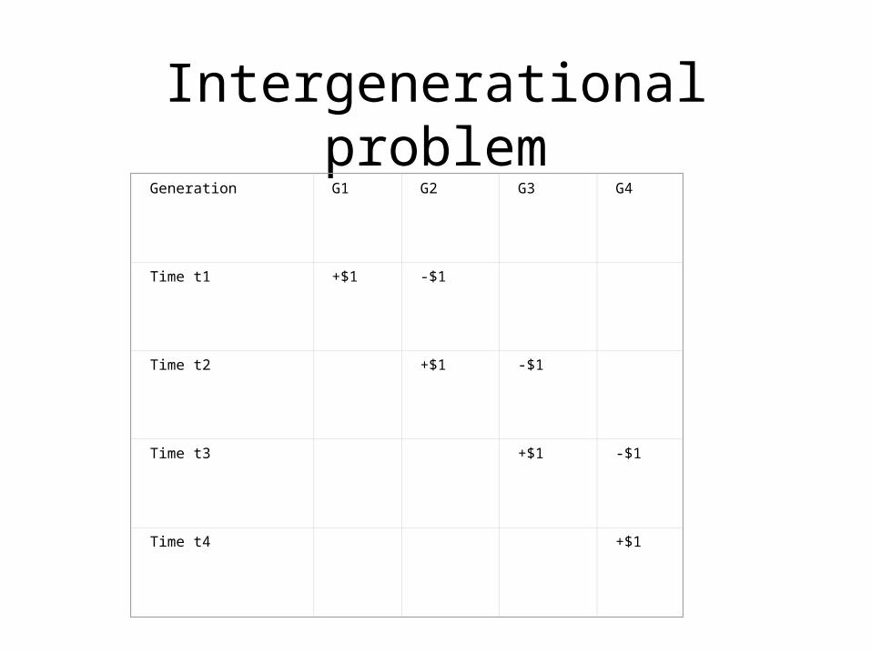
• Each generation lives for two periods (young and old).

• The initial generation (G1) is old at time t1. • They receive $1 per head by taxing

generation G2 at time t1. • Similarly, G2 receives $1 by taxing G3 in

t2. G3, in turn, gets $1 in t3 by taxing G4. • This process continues indefinitely.


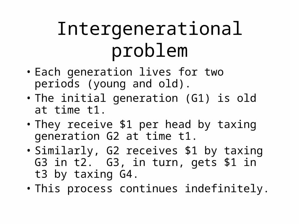
• Let us now consider two systems: pay as you go and a switch to privatized system. We will consider the outcomes in turn.

• Pay as you go: It is easy to see that each generation (except the generation G1) pays $1 in one period and gets $1 in the following period. For example generation G2 pays $1 in t1 and gets $1 in t2. Therefore, the rate of return is zero.


• Privatized scheme: Let us assume that the investors are only allowed to invest in bonds under a privatized individual account system. Let us suppose that the system starts at t2. Suppose the rate of return on the bond is 5%.


• It might seem that the individuals in generation G3 would now get $1.05 in period t3 rather than $1 in the pay as you go regime. Note that the $1 that is owed to G2 has to be paid from somewhere. Suppose that the government pays G2 by selling bonds in t2. The only way the government can sell the bonds is to offer a market interest rate of 5%. In other words, the government owes $1.05 in t3.


• If the government simply wants to keep the principal of the loan at $1, it has to pay for the interest payment in t3. If this five cents ($0.05=$1.05-$1.00) is to be paid for by taxes, it is likely to tax the younger generation. Thus, the net gain of G3 would be $1.05 (from bond holding) minus $0.05 (from tax payment). Thus, once the interest cost (through taxes) is included, G3 does not gain anything from the new privatized system.


• Once the government has borrowed that $1, private accounts do not generate any additional national savings. The $1 extra in private accounts is exactly offset by $1 extra borrowed by the government. With no added savings at the national level, there would be no additional capital formation and therefore no increased wealth for future generations. In future years, nobody in the society will have more income than they would under a pay as you go system.


• The result can be worse for the retired old. If the taxes are paid (at least in part) by the old, they will be worse off. Instead, if the benefits are cut, the retired generation will be worse off as well.


• There is one way of making future generations better off by privatization. Suppose young people direct their $1 contribution to privatized individual accounts. The $1 hole is now "financed" in two parts. The government cuts the benefits of the current old generation by $0.50 and imposes an additional tax of $0.50 to the current young generation. This means no new borrowing is necessary to finance anything else in the future. Future generations will be able to enjoy the 5% without offsetting taxes.


• Of course, there is no free lunch. The above process will make the current old generation worse off. They will see their benefits dwindle by $0.50. In addition, even though the current young people will get a 5% rate of return on their investment, they will also pay an additional tax of $0.50.


• The essential nature of this argument does not change if we have other forms of financing schemes. For example, if all generations hold diversified portfolios (with bonds and stocks), it does not alter the conclusion. The main insight is that higher rates of return for stocks also have higher risk.


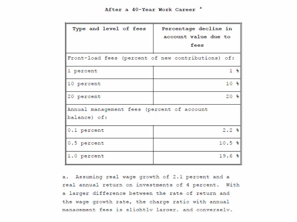
• In summary, privatization of accounts by itself does not have any effect on the economy as a whole. Benefits from privatization only comes from raising taxes or cutting benefits (or both) which might then be used to raise national saving.

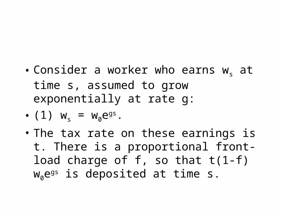
• Consider a worker who earns ws at time s, assumed to grow exponentially at rate g:

• (1) ws = w0egs.

• The tax rate on these earnings is t. There is a proportional front-load charge of f, so that t(1-f) w0egs is deposited at time s.

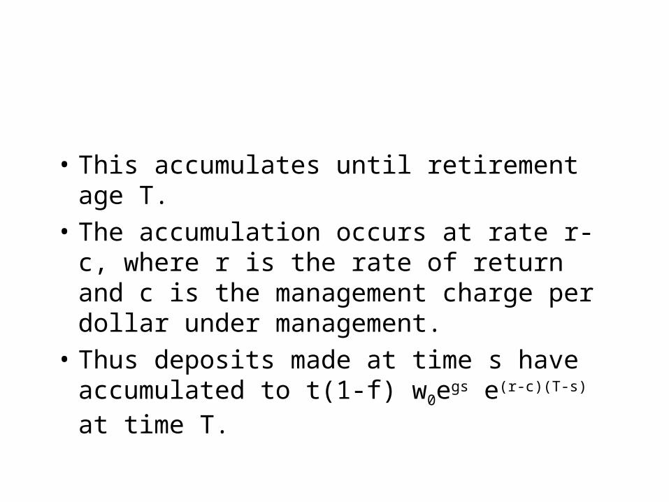
• This accumulates until retirement age T.

• The accumulation occurs at rate r-c, where r is the rate of return and c is the management charge per dollar under management.

• Thus deposits made at time s have accumulated to t(1-f) w0egs e(r-c)(T-s) at time T.

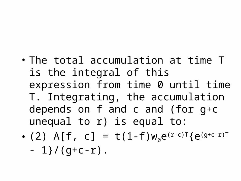
• The total accumulation at time T is the integral of this expression from time 0 until time T. Integrating, the accumulation depends on f and c and (for g+c unequal to r) is equal to:

• (2) A[f, c] = t(1-f)w0e(r-c)T{e(g+c-r)T - 1}/(g+c-r).

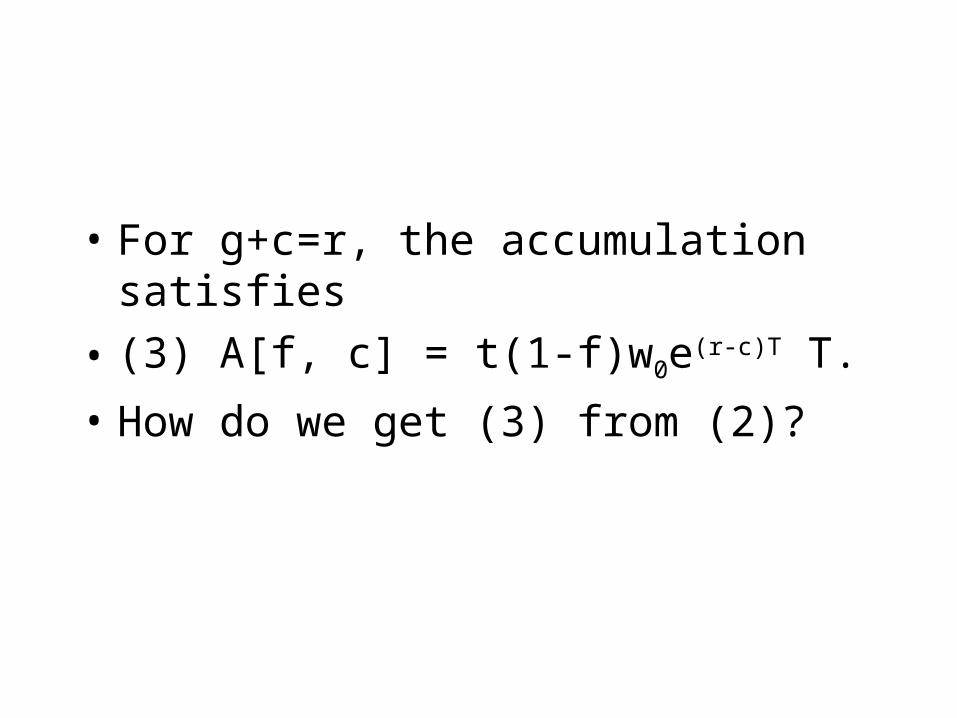
• For g+c=r, the accumulation satisfies

• (3) A[f, c] = t(1-f)w0e(r-c)T T.

• How do we get (3) from (2)?

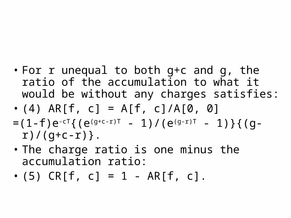
• For r unequal to both g+c and g, the ratio of the accumulation to what it would be without any charges satisfies:

• (4) AR[f, c] = A[f, c]/A[0, 0]=(1-f)e-cT{(e(g+c-r)T - 1)/(e(g-r)T - 1)}{(g-r)/(g+c-r)}.• The charge ratio is one minus the accumulation

ratio:• (5) CR[f, c] = 1 - AR[f, c].

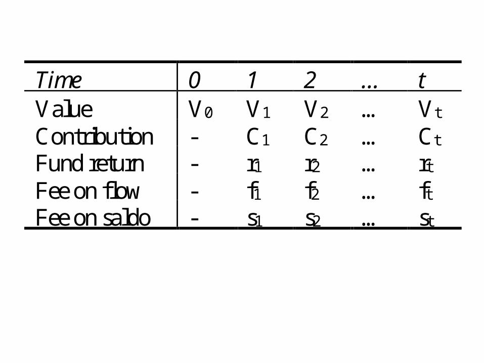
Time 0 1 2 … t Value V0 V1 V2 … Vt Contribution - C1 C2 … Ct Fund return - r1 r2 … rt Fee on flow - f1 f2 … ft Fee on saldo - s1 s2 … st

• Let Vt denote the value of the fund at the

end of time t. The contribution during time t is denoted by Ct (we will assume that the

entire payment occurs at the beginning of the period so that the interest earned by the contribution is the same as interest earned by the balance Vt-1 brought in from the

previous period).

• The rate of return between time t-1 and time t is denoted by rt. There are two types of

fees charged by the AFOREs: fees on flow and fees on saldo. We denote the fee on flow at period t by ft and the fee on saldo at

period t by st.

• Therefore, we can write the value of the fund at time 1 as follows:

• V1 = [V0 + c1(1 - f1)](1 + r1)(1 – s1)• Similarly, the value of the fund at time 2 can be

written as follows:• V2 = [V1 + c2(1 –f2)](1 + r2)(1 – s2)• In general, we can write this recursive relation that

connects period t-1 and t as follows:• Vt = [Vt-1 + ct(1 – ft)](1 + rt)(1 – st)

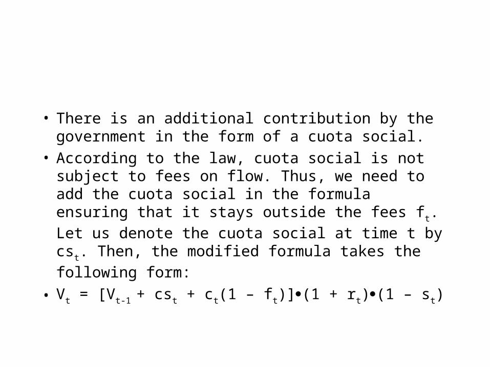
• There is an additional contribution by the government in the form of a cuota social.

• According to the law, cuota social is not subject to fees on flow. Thus, we need to add the cuota social in the formula ensuring that it stays outside the fees ft. Let us denote the cuota social at time t by cst.

Then, the modified formula takes the following form:

• Vt = [Vt-1 + cst + ct(1 – ft)](1 + rt)(1 – st)

• AFORE 2003 Spreadsheet

• Comparison with IMSS

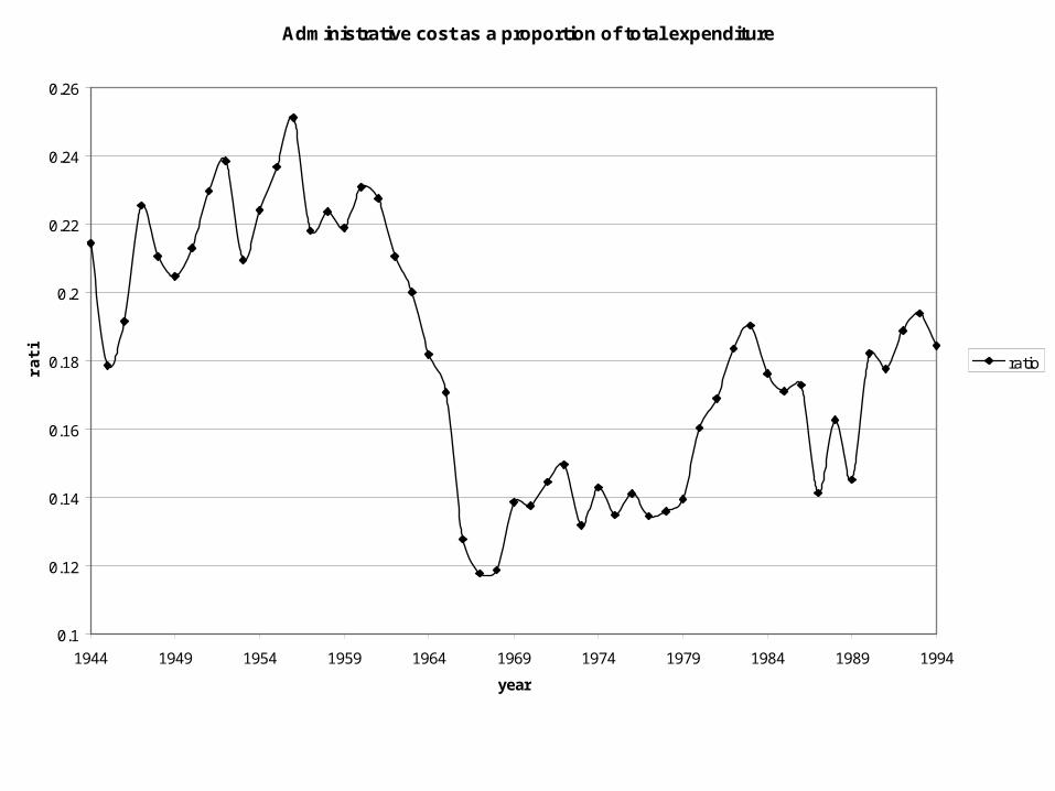
Administrative cost as a proportion of total expenditure

0.1

0.12

0.14

0.16

0.18

0.2

0.22

0.24

0.26

1944 1949 1954 1959 1964 1969 1974 1979 1984 1989 1994

year

rati

o

ratio

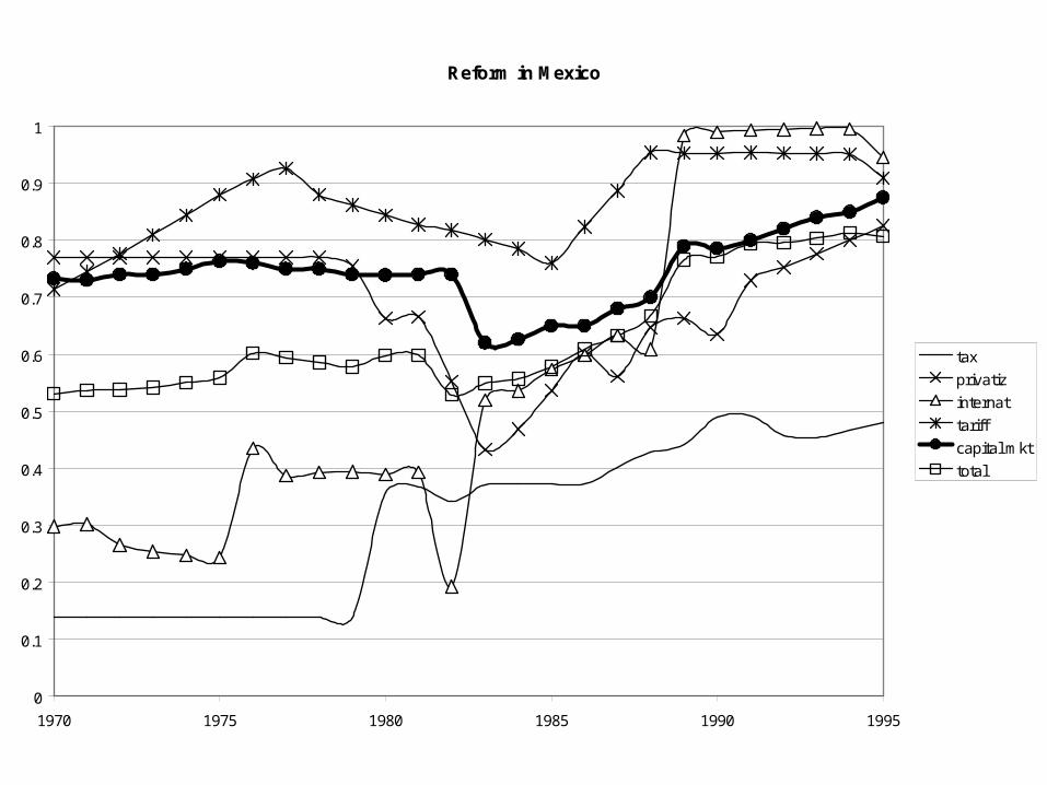
Reform in Mexico

0

0.1

0.2

0.3

0.4

0.5

0.6

0.7

0.8

0.9

1

1970 1975 1980 1985 1990 1995

tax

privatiz

internat

tariff

capital mkt

total

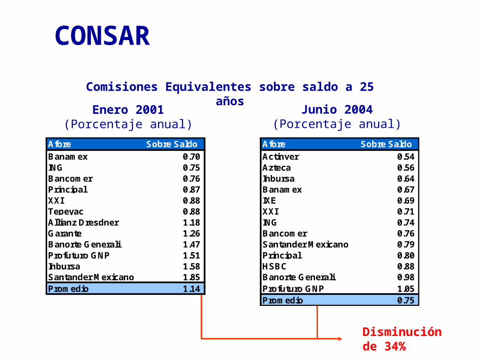
Disminuciónde 34%

CONSAR

Enero 2001(Porcentaje anual)

Junio 2004(Porcentaje anual)

Afore Sobre Saldo Afore Sobre Saldo

Banamex 0.70 Actinver 0.54 ING 0.75 Azteca 0.56 Bancomer 0.76 Inbursa 0.64 Principal 0.87 Banamex 0.67 XXI 0.88 IXE 0.69 Tepeyac 0.88 XXI 0.71 Allianz Dresdner 1.18 ING 0.74 Garante 1.26 Bancomer 0.76 Banorte Generali 1.47 Santander Mexicano 0.79 Profuturo GNP 1.51 Principal 0.80 Inbursa 1.58 HSBC 0.88 Santander Mexicano 1.85 Banorte Generali 0.98 Promedio 1.14 Profuturo GNP 1.05

Promedio 0.75

Comisiones Equivalentes sobre saldo a 25 años

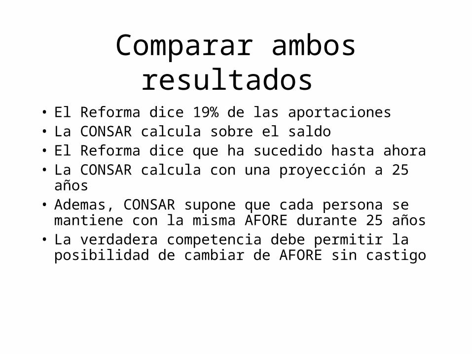
Comparar ambos resultados

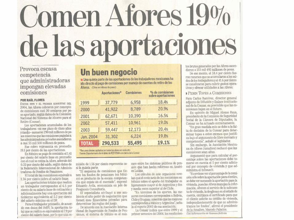
• El Reforma dice 19% de las aportaciones• La CONSAR calcula sobre el saldo• El Reforma dice que ha sucedido hasta ahora• La CONSAR calcula con una proyección a 25

años• Ademas, CONSAR supone que cada persona se

mantiene con la misma AFORE durante 25 años• La verdadera competencia debe permitir la

posibilidad de cambiar de AFORE sin castigo

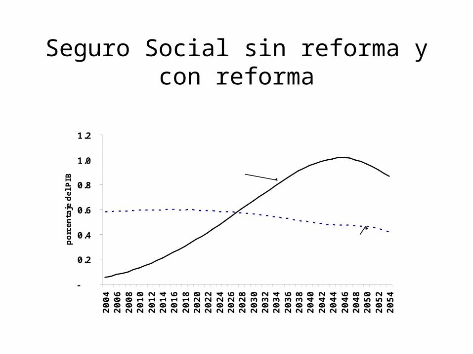
Seguro Social sin reforma y con reforma

-

0.2

0.4

0.6

0.8

1.0

1.2

2004

2006

2008

2010

2012

2014

2016

2018

2020

2022

2024

2026

2028

2030

2032

2034

2036

2038

2040

2042

2044

2046

2048

2050

2052

2054

porc

enta

je d

el P

IB

Sin reforma

Con reforma

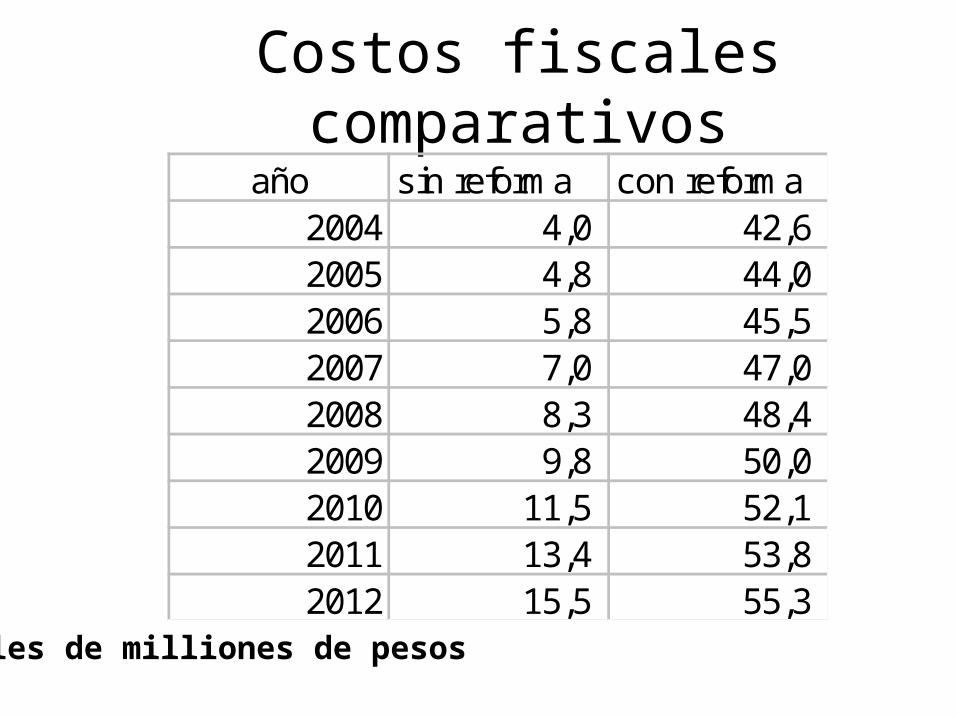
Costos fiscales comparativosaño sin reforma con reforma

2004 4,0 42,6 2005 4,8 44,0 2006 5,8 45,5 2007 7,0 47,0 2008 8,3 48,4 2009 9,8 50,0 2010 11,5 52,1 2011 13,4 53,8 2012 15,5 55,3

Miles de milliones de pesos

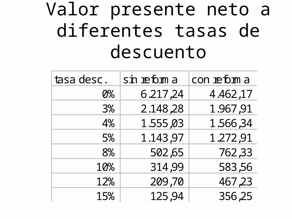
Valor presente neto a diferentes tasas de descuento

tasa desc. sin reforma con reforma0% 6.217,24 4.462,173% 2.148,28 1.967,914% 1.555,03 1.566,345% 1.143,97 1.272,918% 502,65 762,33

10% 314,99 583,5612% 209,70 467,2315% 125,94 356,25

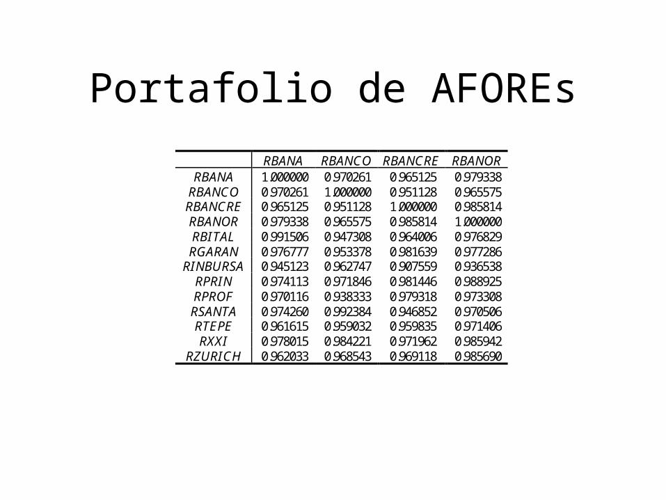
Portafolio de AFOREs

RBANA RBANCO RBANCRE RBANOR RBANA 1.000000 0.970261 0.965125 0.979338

RBANCO 0.970261 1.000000 0.951128 0.965575 RBANCRE 0.965125 0.951128 1.000000 0.985814 RBANOR 0.979338 0.965575 0.985814 1.000000 RBITAL 0.991506 0.947308 0.964006 0.976829 RGARAN 0.976777 0.953378 0.981639 0.977286

RINBURSA 0.945123 0.962747 0.907559 0.936538 RPRIN 0.974113 0.971846 0.981446 0.988925 RPROF 0.970116 0.938333 0.979318 0.973308 RSANTA 0.974260 0.992384 0.946852 0.970506 RTEPE 0.961615 0.959032 0.959835 0.971406 RXXI 0.978015 0.984221 0.971962 0.985942

RZURICH 0.962033 0.968543 0.969118 0.985690

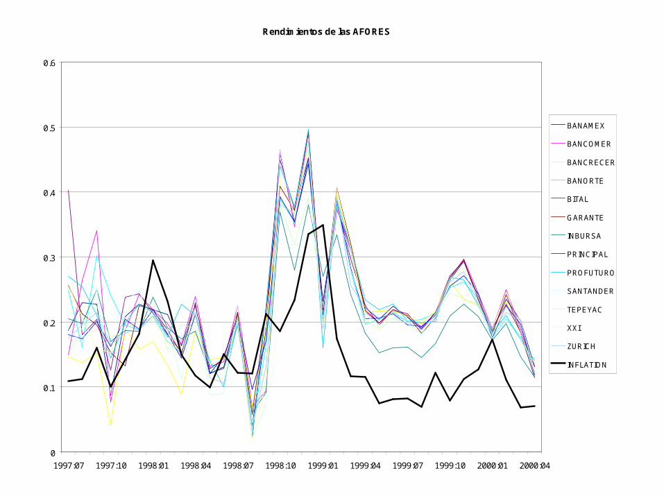
Rendimientos de las AFORES

0

0.1

0.2

0.3

0.4

0.5

0.6

1997:07 1997:10 1998:01 1998:04 1998:07 1998:10 1999:01 1999:04 1999:07 1999:10 2000:01 2000:04

BANAMEX

BANCOMER

BANCRECER

BANORTE

BITAL

GARANTE

INBURSA

PRINCIPAL

PROFUTURO

SANTANDER

TEPEYAC

XXI

ZURICH

INFLATION

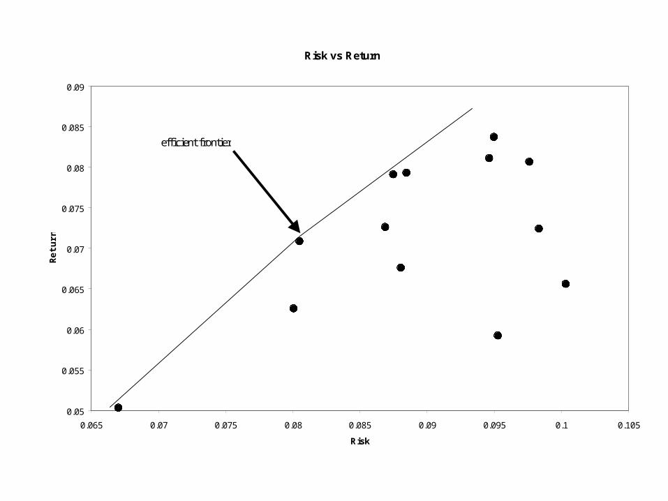
Risk vs Return

0.05

0.055

0.06

0.065

0.07

0.075

0.08

0.085

0.09

0.065 0.07 0.075 0.08 0.085 0.09 0.095 0.1 0.105

Risk

Ret

urn

efficient frontier

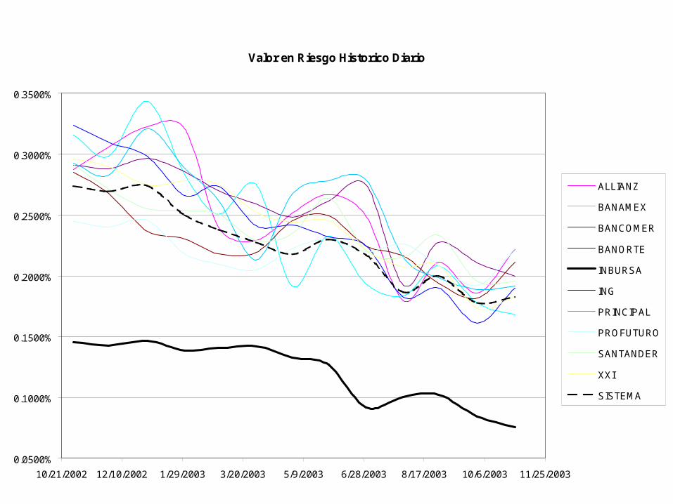
Valor en Riesgo Historico Diario

0.0500%

0.1000%

0.1500%

0.2000%

0.2500%

0.3000%

0.3500%

10/21/2002 12/10/2002 1/29/2003 3/20/2003 5/9/2003 6/28/2003 8/17/2003 10/6/2003 11/25/2003

ALLIANZ

BANAMEX

BANCOMER

BANORTE

INBURSA

ING

PRINCIPAL

PROFUTURO

SANTANDER

XXI

SISTEMA

• Scenario 1: Affiliate with three minimum salary (flat profile with the assumption of the salario minimo at 16,931 per year), 5% real interest rate (we assume it is the same for all AFORES), 0% inflation, 0 initial quantity brought into the system

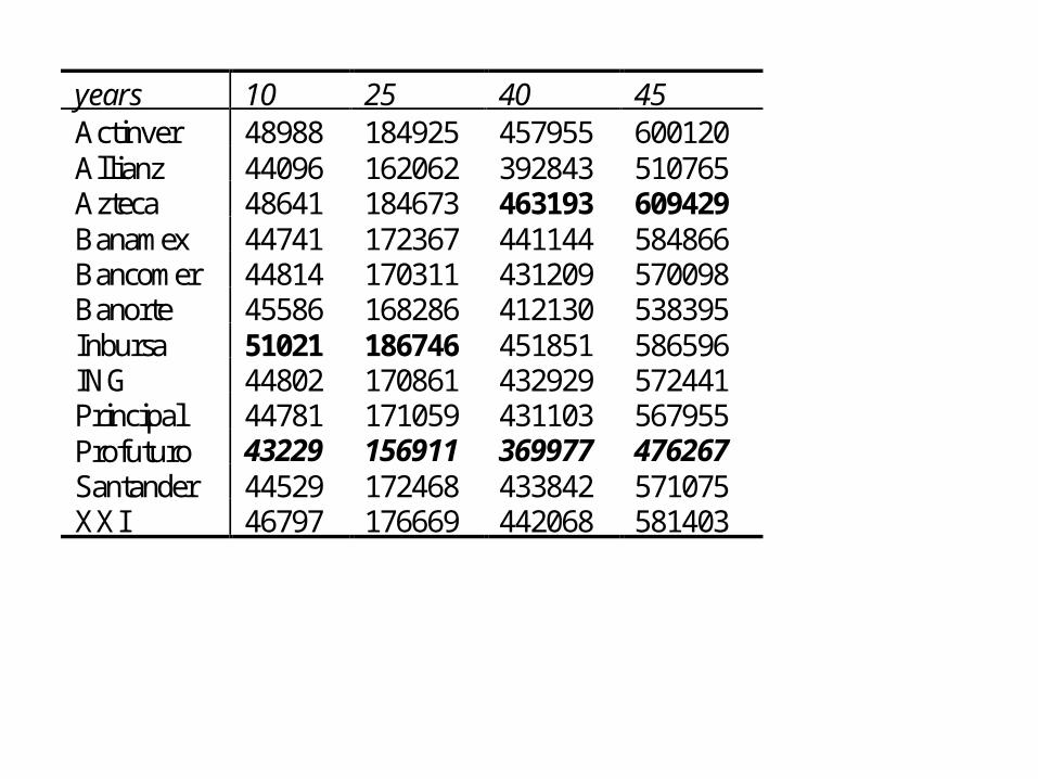
years 10 25 40 45 Actinver 48988 184925 457955 600120 Allianz 44096 162062 392843 510765 Azteca 48641 184673 463193 609429 Banamex 44741 172367 441144 584866 Bancomer 44814 170311 431209 570098 Banorte 45586 168286 412130 538395 Inbursa 51021 186746 451851 586596 ING 44802 170861 432929 572441 Principal 44781 171059 431103 567955 Profuturo 43229 156911 369977 476267 Santander 44529 172468 433842 571075 XXI 46797 176669 442068 581403

• Scenario 2: Suppose we keep all the other assumptions the same as in scenario 1 but simply change the amount of money an affiliate brings into the system. (3 times salario minimo and 5% real return with 0% inflation but an initial amount of 50,000.)

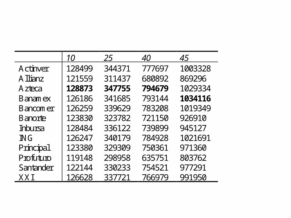
10 25 40 45 Actinver 128499 344371 777697 1003328 Allianz 121559 311437 680892 869296 Azteca 128873 347755 794679 1029334 Banamex 126186 341685 793144 1034116 Bancomer 126259 339629 783208 1019349 Banorte 123830 323782 721150 926910 Inbursa 128484 336122 739899 945127 ING 126247 340179 784928 1021691 Principal 123380 329309 750361 971360 Profuturo 119148 298958 635751 803762 Santander 122144 330233 754521 977291 XXI 126628 337721 766979 991950

• Impact of the real interest rate: If the real interest rate is high and stays high (for example, 10%), the charges of Inbursa begin to have a bigger bite by the twenty-seventh year. Azteca becomes the best AFORE.

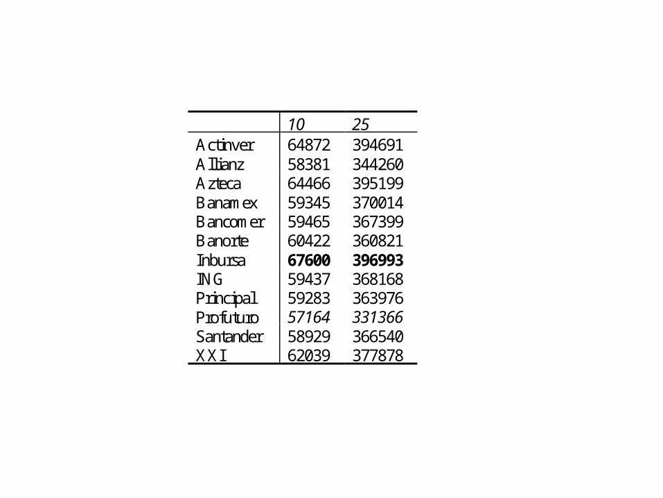
10 25 Actinver 64872 394691 Allianz 58381 344260 Azteca 64466 395199 Banamex 59345 370014 Bancomer 59465 367399 Banorte 60422 360821 Inbursa 67600 396993 ING 59437 368168 Principal 59283 363976 Profuturo 57164 331366 Santander 58929 366540 XXI 62039 377878

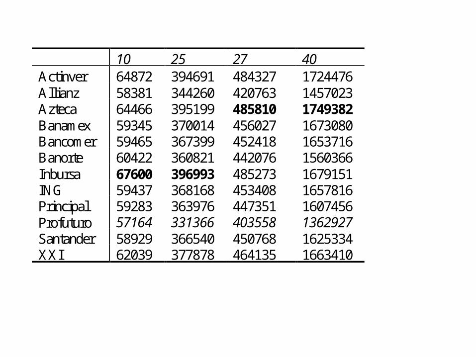
10 25 27 40 Actinver 64872 394691 484327 1724476 Allianz 58381 344260 420763 1457023 Azteca 64466 395199 485810 1749382 Banamex 59345 370014 456027 1673080 Bancomer 59465 367399 452418 1653716 Banorte 60422 360821 442076 1560366 Inbursa 67600 396993 485273 1679151 ING 59437 368168 453408 1657816 Principal 59283 363976 447351 1607456 Profuturo 57164 331366 403558 1362927 Santander 58929 366540 450768 1625334 XXI 62039 377878 464135 1663410

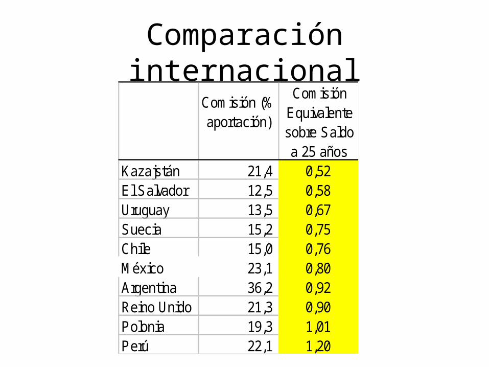
Comparación internacional

Comisión (% aportación)

Comisión Equivalente sobre Saldo a 25 años

Kazajstán 21,4 0,52 El Salvador 12,5 0,58 Uruguay 13,5 0,67 Suecia 15,2 0,75 Chile 15,0 0,76 México 23,1 0,80 Argentina 36,2 0,92 Reino Unido 21,3 0,90 Polonia 19,3 1,01 Perú 22,1 1,20

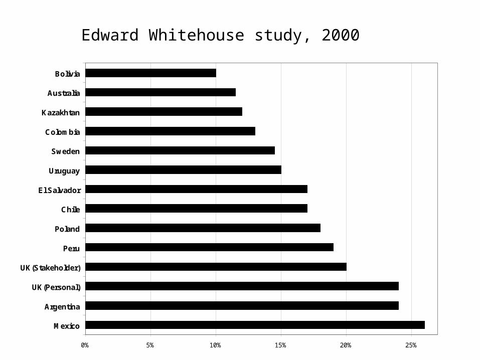
0% 5% 10% 15% 20% 25%

Mexico

Argentina

UK(Personal)

UK(Stakeholder)

Peru

Poland

Chile

El Salvador

Uruguay

Sweden

Colombia

Kazakhtan

Australia

Bolivia

Edward Whitehouse study, 2000

Intergenerational problem

Documents

Transcript of Intergenerational problem