
Interfacial Tension of Reservoir Fluids: an Integrated ...
239
Interfacial Tension of Reservoir Fluids: an Integrated Experimental and Modelling Investigation by Luís M. C. Pereira Thesis submitted for the degree of Doctor of Philosophy in Petroleum Engineering School of Energy, Geoscience, Infrastructure and Society Heriot-Watt University July 2016 The copyright in this thesis is owned by the author. Any quotation from the thesis or use of any of the information contained in it must acknowledge this thesis as the source of the quotation or information.
Transcript of Interfacial Tension of Reservoir Fluids: an Integrated ...
Interfacial Tension of Reservoir Fluids: an
Integrated Experimental and Modelling
Investigation
by
Luís M. C. Pereira
Thesis submitted for the degree of Doctor of Philosophy in
Petroleum Engineering
School of Energy, Geoscience, Infrastructure and Society
Heriot-Watt University
July 2016
The copyright in this thesis is owned by the author. Any quotation from the thesis or use
of any of the information contained in it must acknowledge this thesis as the source of the
quotation or information.

PREFACE
The work presented in this manuscript has been developed as part of my PhD studies at
Heriot-Watt University (HWU) under the supervision of Prof. Bahman Tohidi and Dr.
Antonin Chapoy, between January 2013 and June 2016. The research described here was
performed in the context of a Joint Industrial Project conducted in the Gas Hydrates, Flow
Assurance and Phase Equilibria research group at HWU. Phase behaviour models
implemented in the in-house PVT software of this research group (HWPVT) were used
throughout this work. Part of the material in this manuscript has been presented or
published elsewhere before; the list of publications concerning the studies described in
this manuscript is given in LIST OF PUBLICATIONS BY THE CANDIDATE.
Luís Pereira
July 2016
ABSTRACT
Interfacial tension (IFT) is a property of paramount importance in many technical areas
as it deals with the forces acting at the interface whenever two immiscible or partially
miscible phases are in contact. With respect to petroleum engineering operations, it
influences most, if not all, multiphase processes associated with the extraction and
refining of Oil and Gas, from the optimisation of reservoir engineering strategies to the
design of petrochemical facilities. This property is also of key importance for the
development of successful and economical CO2 geological storage projects as it controls,
to a large extent, the amount of CO2 that can be safely stored in a target reservoir.
Therefore, an accurate knowledge of the IFT of reservoir fluids is needed.
Aiming at filling the experimental gap found in literature and extending the measurement
of this property to reservoir conditions, the present work contributes with fundamental
IFT data of binary and multicomponent synthetic reservoir fluids. Two new setups have
been developed, validated and used to study the impact of high pressures (up to 69 MPa)
and high temperatures (up to 469 K) on the IFT of hydrocarbon systems including
n-alkanes and main gas components such as CH4, CO2, and N2, as well as of the effect
sparingly soluble gaseous impurities and NaCl on the IFT of water and CO2 systems.
Saturated density data of the phases, required to determine pertinent IFT values, have also
been measured with a vibrating U-tube densitometer. Results indicated a strong
dependence of the IFT values with temperature, pressure, phase density and salt
concentration, whereas changes on the IFT due to the presence of up to 10 mole% gaseous
impurities (sparingly soluble in water) laid very close to experimental uncertainties.
Additionally, the predictive capabilities of classical methods for computing IFT values
have been compared to a more robust theoretical approach, the Density Gradient Theory
(DGT), as well as to experimental data measured in this work and collected from
literature. Results demonstrated the superior capabilities of the DGT for accurately
predicting the IFT of synthetic hydrocarbon mixtures and of a real petroleum fluid with
no further adjustable parameters for mixtures. In the case of aqueous systems, one binary
interaction coefficient, estimated with the help of a single experimental data point,
allowed the correct description of the IFT of binary and multicomponent systems in both
two- and three-phase equilibria conditions, as well as the impact of salts with the DGT.

Aos meus pais, pelo amor incondicional e educação.

ACKNOWLEDGMENTS
This work would have been impossible without the help, support and contributions of all
the people that were around me during these three and a half years and for which I will
forever be grateful.
First, I would like to thank Prof. Bahman Tohidi for having given me the opportunity to
conduct my PhD studies in his group, for what I have learnt with him and for his guidance
throughout these years. Special and countless thanks are owed to Dr. Antonin Chapoy
for his much valued inputs towards my research, for his support and for his seemingly
limitless patience; this work is much indebted to him. I cannot forget also the help and
assistance given by Dr. Rod Burgass in the laboratory and by Mr. Jim Allinson and Mr.
Jack Irvine during the design and construction of the experimental setups used in this
work. Moreover, I specially appreciate the financial support received from GALP
Energia through my scholarship. Last but foremost, I am extremely grateful to Prof. João
Coutinho, my MSc supervisor, for believing that I was up to the challenge, for sharing
with me his knowledge of thermodynamics, and most importantly, life lessons that made
a better “me”, and for all the invaluable discussions we had.
I had the privilege of sharing the office with fantastic people, each one with unique ways
of companionship, and to have met friends who were the source of revitalization outside
the working hours. For their friendship, dinners and adventures we shared together, I am
truly grateful to Alfonso (Fon), Foroogh, Anthony, Duarte, Wissem, Mohamed, Bouja,
Morteza, Mohammadreza, Edris, Diana and Martha. An extra special thank must go to
Fon, who, with his fonsenglish and excellent mathematical knowledge, among many
others talents, was always there not only to cheer me up, but also to help me overcome
the obstacles and tackle the problems that arose during an important period of my PhD.
Words cannot express my gratitude to my long-term companion, Ana, for her love and
her patience (most of the time), to her goes my biggest Thank You.

Please note this form should bound into the submitted thesis.
Updated February 2008, November 2008, February 2009, January 2011
ACADEMIC REGISTRY Research Thesis Submission
Name: Luís Manuel Cravo Pereira
School/PGI: School of Energy, Geoscience, Infrastructure and Society
Version: (i.e. First,
Resubmission, Final) Final Degree Sought
(Award and Subject area)
PhD
Petroleum Engineering
Declaration In accordance with the appropriate regulations I hereby submit my thesis and I declare that:
1) the thesis embodies the results of my own work and has been composed by myself 2) where appropriate, I have made acknowledgement of the work of others and have made reference to
work carried out in collaboration with other persons 3) the thesis is the correct version of the thesis for submission and is the same version as any electronic
versions submitted*. 4) my thesis for the award referred to, deposited in the Heriot-Watt University Library, should be made
available for loan or photocopying and be available via the Institutional Repository, subject to such conditions as the Librarian may require
5) I understand that as a student of the University I am required to abide by the Regulations of the University and to conform to its discipline.
* Please note that it is the responsibility of the candidate to ensure that the correct version of the thesis is
submitted.
Signature of Candidate:
Date: 25/07/2016
Submission
Submitted By (name in capitals):
Signature of Individual Submitting:
Date Submitted:
For Completion in the Student Service Centre (SSC)
Received in the SSC by (name in
capitals):
Method of Submission (Handed in to SSC; posted through internal/external mail):
E-thesis Submitted (mandatory for
final theses)
Signature:
Date:
i
TABLE OF CONTENTS
LIST OF PUBLICATIONS BY THE CANDIDATE iii
LIST OF TABLES v
LIST OF FIGURES viii
NOMENCLATURE xv
INTRODUCTION 1
Background 1 Thesis Objectives 2 Thesis Outline 2
CHAPTER 1 – INTERFACIAL TENSION 3
1.1 Fundamentals 3 1.2 Significance of Fluid−Liquid Interfacial Tensions 7 1.3 Literature Survey 11
1.3.1 Hydrocarbon systems 11
1.3.2 Aqueous systems 14 1.4 Summary 20
CHAPTER 2 – EXPERIMENTAL TECHNIQUES FOR MEASURING
INTERFACIAL TENSION 21
2.1 Introduction 21 2.2 Capillary Rise Technique 22
2.2.1 Generalities 22 2.2.2 Experimental setup 26
2.3 Pendant Drop Technique 29 2.3.1 Generalities 29
2.3.2 Experimental setup 32 2.4 Summary 36
CHAPTER 3 – THERMODYNAMIC MODELLING OF INTERFACIAL
TENSION 37
3.1 Introduction 37 3.2 Parachor Method 38 3.3 Sutton’s Correlation 40
3.4 Density Gradient Theory 42 3.4.1 Theory outline 42
3.4.2 Influence parameter 45 3.4.3 Molecular distribution across a planar interface 52
3.5 Linear Gradient Theory 56 3.6 Phase Behaviour Model 57 3.7 Summary 61
CHAPTER 4 – INTERFACIAL TENSION OF HYDROCARBON SYSTEMS 63
4.1 Introduction 63 4.2 Experimental Procedure 64
4.2.1 Materials and sample preparation 64 4.2.2 Measuring procedure 65
4.3 Experimental Results 68
ii
4.3.1 Binary mixtures 68 4.3.2 Multicomponent mixtures 72
4.3.3 Experimental uncertainties 74 4.4 Modelling 75
4.4.1 Binary and multicomponent synthetic mixtures 75 4.4.2 Real Black oil 82
4.5 Microstructure of Interfaces 92 4.6 Summary 94
CHAPTER 5 – INTERFACIAL TENSION OF AQUEOUS SYSTEMS 96
5.1 Introduction 96 5.2 Experimental Procedure 97
5.2.1 Materials and sample preparation 97 5.2.2 Measuring procedure 98
5.3 Experimental Results 100
5.3.1 CO2 and H2O 100 5.3.2 CO2-rich mixtures and water 108 5.3.3 CO2 and NaCl brines 110 5.3.4 Experimental uncertainties 114
5.3.5 Implications on the geological storage of CO2 114 5.4 Modelling 119
5.4.1 Binary mixtures 119 5.4.2 Multicomponent mixtures 132
5.5 Microstructure of Interfaces 146 5.6 Summary 154
CHAPTER 6 – CONCLUSIONS AND RECOMMENDATIONS FOR FUTURE
WORK 158
6.1 Introduction 158 6.2 Experimental Investigation 158 6.3 Modelling Investigation 161
6.4 Recommendations for Future Work 163
APPENDIX A Peng-Robinson 1978 Equation of State 167
APPENDIX B Cubic-Plus-Association Equation of State 168
APPENDIX C Optimized Binary Interaction Coefficients and Volume
Corrections for the Correlation of Saturated Density Data with the PR78 EoS 170
APPENDIX D Saturated Density Data 171
APPENDIX E Interfacial Tension Data 178
APPENDIX F Complementary Modelling Results 188
REFERENCES 193
iii
LIST OF PUBLICATIONS BY THE CANDITATE
L.M.C. Pereira, A. Chapoy, R. Burgass, B. Tohidi, Interfacial tension of CO2 + brine
systems under geological sequestration conditions: experiments, modelling and
implications, (in preparation).
L.M.C. Pereira, A. Chapoy, R. Burgass, B. Tohidi, Measurement and modelling of high
pressure density and interfacial tension of (gas + n-alkane) binary mixtures, J. Chem.
Thermodyn. 97, 55–69 (2016).
K. Kashefi, L.M.C. Pereira, A. Chapoy, R. Burgass, B. Tohidi, Measurement and
modelling of interfacial tension in methane/water and methane/brine systems at reservoir
conditions, Fluid Phase Equilib. 409, 301–311 (2016).
L.M.C. Pereira, A. Chapoy, R. Burgass, M.B. Oliveira, J.A.P. Coutinho, B. Tohidi,
Study of the impact of high temperatures and pressures on the equilibrium densities and
interfacial tension of the carbon dioxide/water system, J. Chem. Thermodyn. 93, 404–
415 (2016). Part of the special issue of JCT on Thermophysical Properties for Carbon
Dioxide Transportation and Storage.
L.M.C. Pereira, A. Chapoy, B. Tohidi, Modelling of CO2/brine interfacial tensions
under CO2 geological storage conditions, presented (poster) in Scottish Carbon Capture
& Storage Conference, Edinburgh, UK (2015).
A. Gonzalez, L. Pereira, P. Paricaud, C. Coquelet, A. Chapoy, Modeling of transport
properties using the SAFT-VR Mie equation of state, published and presented (oral) in
SPE Annual Technical Conference and Exhibition (Paper # SPE-175051-MS), Houston,
Texas, USA (2015).
L.M.C. Pereira, A. Chapoy, B. Tohidi, Vapor-liquid and liquid-liquid interfacial tension
of water and hydrocarbon systems at representative reservoir conditions: experimental
and modeling results, published and presented (oral) in SPE Annual Technical
Conference and Exhibition (Paper # SPE-170670-MS), Amsterdam, The Netherlands
(2014).
L.M.C. Pereira, A. Chapoy, B. Tohidi, Interfacial tension studies in CO2-rich mixtures
at representative reservoir conditions, published and presented (oral) in Rio Oil & Gas
Expo and Conference (Paper # IBP 1902_14), Rio de Janeiro, Brazil (2014).

iv
L. Pereira, A. Chapoy, B. Tohidi, A comprehensive study of the impact of elevated
temperatures and pressures on the interfacial tension of the carbon dioxide/water system,
presented (oral) in the 20th European Conference on Thermophysical Properties, Porto,
Portugal (2014).
L. Pereira, M. Kapateh, A. Chapoy, Impact of impurities on thermophysical properties
and dehydration requirements of CO2-rich systems, presented (oral) in UKCCSRC
Biannual Meeting, Cambridge, UK (2014).
v
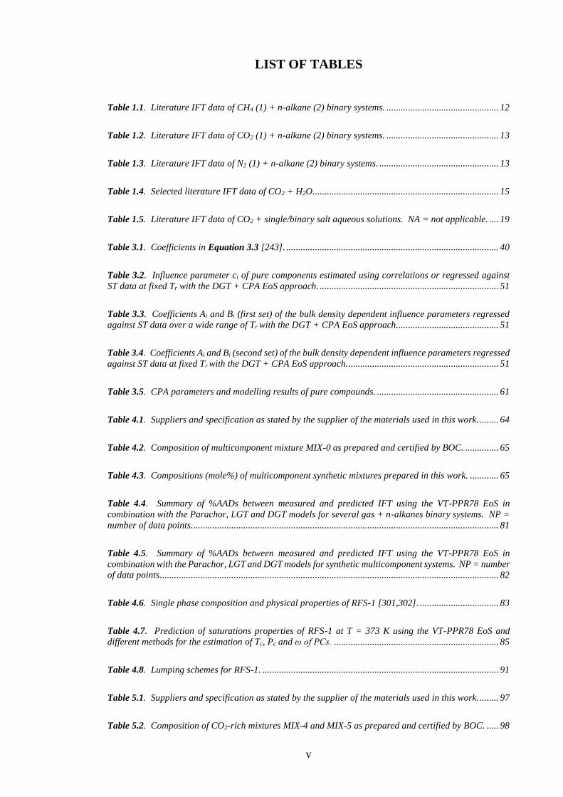
LIST OF TABLES
Table 1.1. Literature IFT data of CH4 (1) + n-alkane (2) binary systems. ............................................... 12
Table 1.2. Literature IFT data of CO2 (1) + n-alkane (2) binary systems. ............................................... 13
Table 1.3. Literature IFT data of N2 (1) + n-alkane (2) binary systems. .................................................. 13
Table 1.4. Selected literature IFT data of CO2 + H2O. ............................................................................. 15
Table 1.5. Literature IFT data of CO2 + single/binary salt aqueous solutions. NA = not applicable. .... 19
Table 3.1. Coefficients in Equation 3.3 [243]. ......................................................................................... 40
Table 3.2. Influence parameter ci of pure components estimated using correlations or regressed against
ST data at fixed Tr with the DGT + CPA EoS approach. ........................................................................... 51
Table 3.3. Coefficients Ai and Bi (first set) of the bulk density dependent influence parameters regressed
against ST data over a wide range of Tr with the DGT + CPA EoS approach. .......................................... 51
Table 3.4. Coefficients Ai and Bi (second set) of the bulk density dependent influence parameters regressed
against ST data at fixed Tr with the DGT + CPA EoS approach. ............................................................... 51
Table 3.5. CPA parameters and modelling results of pure compounds. ................................................... 61
Table 4.1. Suppliers and specification as stated by the supplier of the materials used in this work. ........ 64
Table 4.2. Composition of multicomponent mixture MIX-0 as prepared and certified by BOC. .............. 65
Table 4.3. Compositions (mole%) of multicomponent synthetic mixtures prepared in this work. ............ 65
Table 4.4. Summary of %AADs between measured and predicted IFT using the VT-PPR78 EoS in
combination with the Parachor, LGT and DGT models for several gas + n-alkanes binary systems. NP =
number of data points. ................................................................................................................................ 81
Table 4.5. Summary of %AADs between measured and predicted IFT using the VT-PPR78 EoS in
combination with the Parachor, LGT and DGT models for synthetic multicomponent systems. NP = number
of data points. ............................................................................................................................................. 82
Table 4.6. Single phase composition and physical properties of RFS-1 [301,302]. ................................. 83
Table 4.7. Prediction of saturations properties of RFS-1 at T = 373 K using the VT-PPR78 EoS and
different methods for the estimation of Tc, Pc and ω of PCs. ..................................................................... 85
Table 4.8. Lumping schemes for RFS-1. ................................................................................................... 91
Table 5.1. Suppliers and specification as stated by the supplier of the materials used in this work. ........ 97
Table 5.2. Composition of CO2-rich mixtures MIX-4 and MIX-5 as prepared and certified by BOC. ..... 98
vi
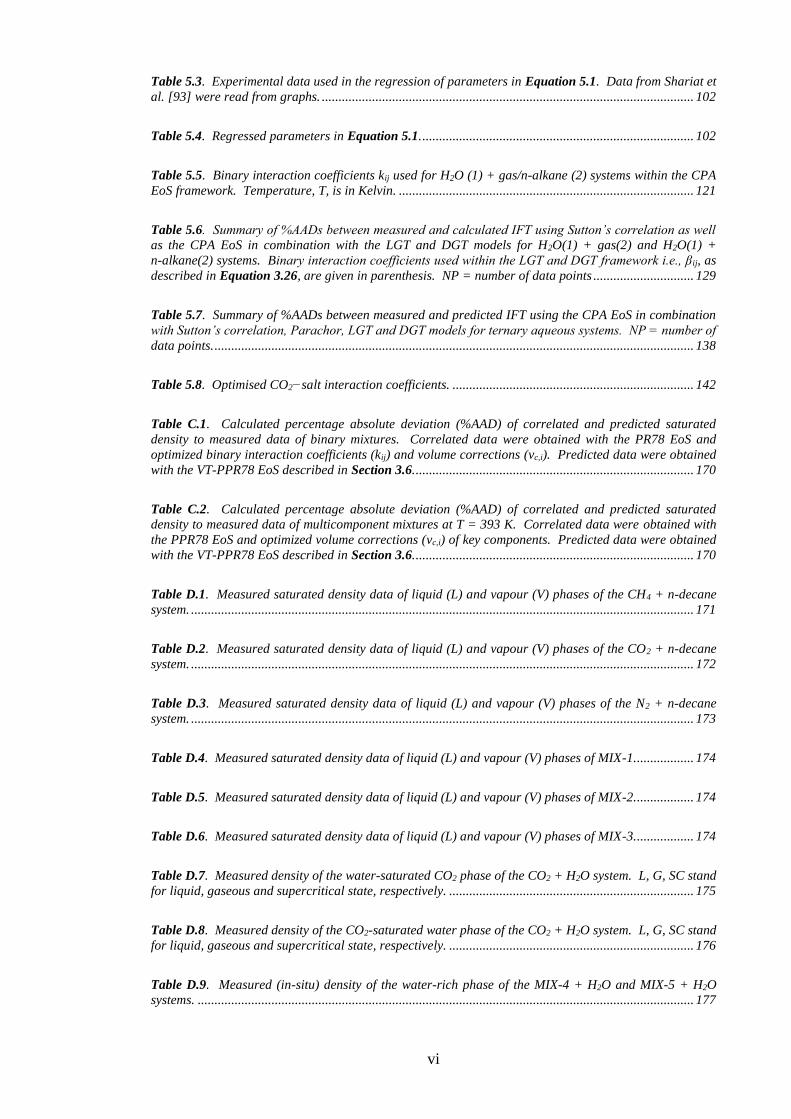
Table 5.3. Experimental data used in the regression of parameters in Equation 5.1. Data from Shariat et
al. [93] were read from graphs. ............................................................................................................... 102
Table 5.4. Regressed parameters in Equation 5.1. ................................................................................. 102
Table 5.5. Binary interaction coefficients kij used for H2O (1) + gas/n-alkane (2) systems within the CPA
EoS framework. Temperature, T, is in Kelvin. ........................................................................................ 121
Table 5.6. Summary of %AADs between measured and calculated IFT using Sutton’s correlation as well
as the CPA EoS in combination with the LGT and DGT models for H2O(1) + gas(2) and H2O(1) +
n-alkane(2) systems. Binary interaction coefficients used within the LGT and DGT framework i.e., βij, as
described in Equation 3.26, are given in parenthesis. NP = number of data points .............................. 129
Table 5.7. Summary of %AADs between measured and predicted IFT using the CPA EoS in combination
with Sutton’s correlation, Parachor, LGT and DGT models for ternary aqueous systems. NP = number of
data points. ............................................................................................................................................... 138
Table 5.8. Optimised CO2−salt interaction coefficients. ........................................................................ 142
Table C.1. Calculated percentage absolute deviation (%AAD) of correlated and predicted saturated
density to measured data of binary mixtures. Correlated data were obtained with the PR78 EoS and
optimized binary interaction coefficients (kij) and volume corrections (vc,i). Predicted data were obtained
with the VT-PPR78 EoS described in Section 3.6. ................................................................................... 170
Table C.2. Calculated percentage absolute deviation (%AAD) of correlated and predicted saturated
density to measured data of multicomponent mixtures at T = 393 K. Correlated data were obtained with
the PPR78 EoS and optimized volume corrections (vc,i) of key components. Predicted data were obtained
with the VT-PPR78 EoS described in Section 3.6. ................................................................................... 170
Table D.1. Measured saturated density data of liquid (L) and vapour (V) phases of the CH4 + n-decane
system. ...................................................................................................................................................... 171
Table D.2. Measured saturated density data of liquid (L) and vapour (V) phases of the CO2 + n-decane
system. ...................................................................................................................................................... 172
Table D.3. Measured saturated density data of liquid (L) and vapour (V) phases of the N2 + n-decane
system. ...................................................................................................................................................... 173
Table D.4. Measured saturated density data of liquid (L) and vapour (V) phases of MIX-1. ................. 174
Table D.5. Measured saturated density data of liquid (L) and vapour (V) phases of MIX-2. ................. 174
Table D.6. Measured saturated density data of liquid (L) and vapour (V) phases of MIX-3. ................. 174
Table D.7. Measured density of the water-saturated CO2 phase of the CO2 + H2O system. L, G, SC stand
for liquid, gaseous and supercritical state, respectively. ......................................................................... 175
Table D.8. Measured density of the CO2-saturated water phase of the CO2 + H2O system. L, G, SC stand
for liquid, gaseous and supercritical state, respectively. ......................................................................... 176
Table D.9. Measured (in-situ) density of the water-rich phase of the MIX-4 + H2O and MIX-5 + H2O
systems. .................................................................................................................................................... 177
vii
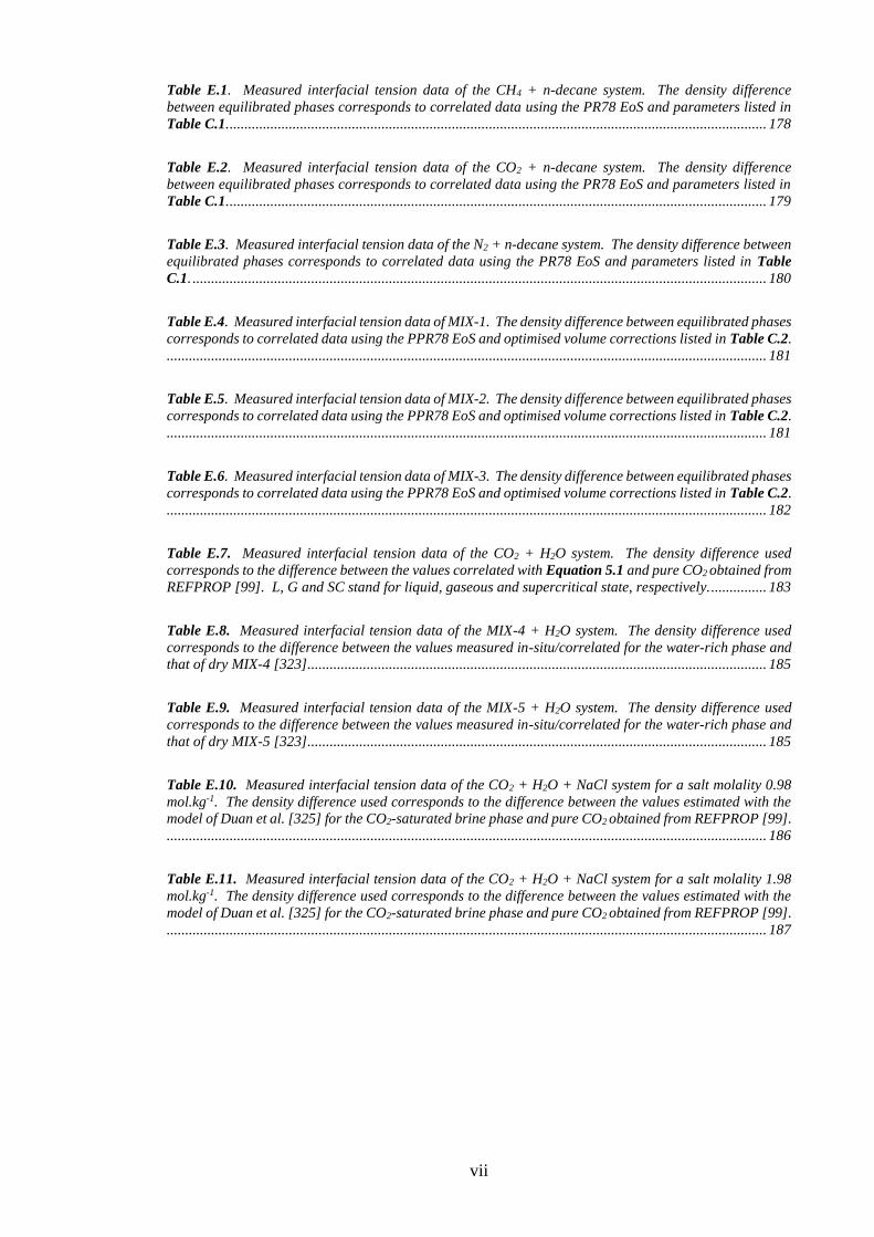
Table E.1. Measured interfacial tension data of the CH4 + n-decane system. The density difference
between equilibrated phases corresponds to correlated data using the PR78 EoS and parameters listed in
Table C.1. ................................................................................................................................................. 178
Table E.2. Measured interfacial tension data of the CO2 + n-decane system. The density difference
between equilibrated phases corresponds to correlated data using the PR78 EoS and parameters listed in
Table C.1. ................................................................................................................................................. 179
Table E.3. Measured interfacial tension data of the N2 + n-decane system. The density difference between
equilibrated phases corresponds to correlated data using the PR78 EoS and parameters listed in Table
C.1. ........................................................................................................................................................... 180
Table E.4. Measured interfacial tension data of MIX-1. The density difference between equilibrated phases
corresponds to correlated data using the PPR78 EoS and optimised volume corrections listed in Table C.2.
.................................................................................................................................................................. 181
Table E.5. Measured interfacial tension data of MIX-2. The density difference between equilibrated phases
corresponds to correlated data using the PPR78 EoS and optimised volume corrections listed in Table C.2.
.................................................................................................................................................................. 181
Table E.6. Measured interfacial tension data of MIX-3. The density difference between equilibrated phases
corresponds to correlated data using the PPR78 EoS and optimised volume corrections listed in Table C.2.
.................................................................................................................................................................. 182
Table E.7. Measured interfacial tension data of the CO2 + H2O system. The density difference used
corresponds to the difference between the values correlated with Equation 5.1 and pure CO2 obtained from
REFPROP [99]. L, G and SC stand for liquid, gaseous and supercritical state, respectively. ............... 183
Table E.8. Measured interfacial tension data of the MIX-4 + H2O system. The density difference used
corresponds to the difference between the values measured in-situ/correlated for the water-rich phase and
that of dry MIX-4 [323]. ........................................................................................................................... 185
Table E.9. Measured interfacial tension data of the MIX-5 + H2O system. The density difference used
corresponds to the difference between the values measured in-situ/correlated for the water-rich phase and
that of dry MIX-5 [323]. ........................................................................................................................... 185
Table E.10. Measured interfacial tension data of the CO2 + H2O + NaCl system for a salt molality 0.98
mol.kg-1. The density difference used corresponds to the difference between the values estimated with the
model of Duan et al. [325] for the CO2-saturated brine phase and pure CO2 obtained from REFPROP [99].
.................................................................................................................................................................. 186
Table E.11. Measured interfacial tension data of the CO2 + H2O + NaCl system for a salt molality 1.98
mol.kg-1. The density difference used corresponds to the difference between the values estimated with the
model of Duan et al. [325] for the CO2-saturated brine phase and pure CO2 obtained from REFPROP [99].
.................................................................................................................................................................. 187
viii
LIST OF FIGURES
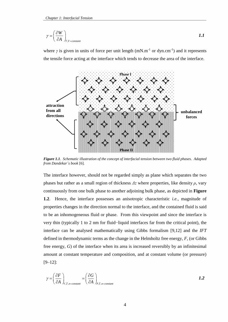
Figure 1.1. Schematic illustration of the concept of interfacial tension between two fluid phases. Adapted
from Dandekar´s book [6]............................................................................................................................ 4
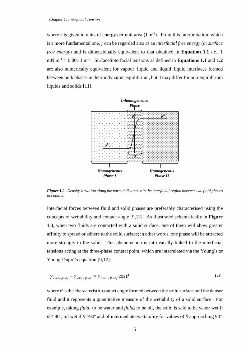
Figure 1.2. Density variation along the normal distance z in the interfacial region between two fluid phases
in contact. ..................................................................................................................................................... 5
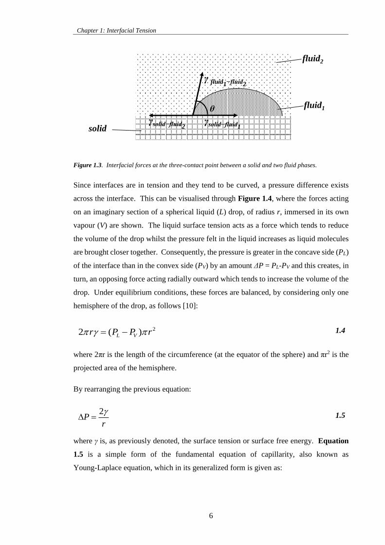
Figure 1.3. Interfacial forces at the three-contact point between a solid and two fluid phases. ................ 6
Figure 1.4. Direction of forces acting on an imaginary section of one hemisphere of a spherical liquid
drop immersed in its own vapour. Adapted from Pellicer et al. [10]. ......................................................... 7
Figure 1.5. IFT-pressure diagram of CO2 + H2O and CO2 + H2O + Salt systems. IFT data reported by
Georgiadis et al. [91] were recalculated using the correlation developed in this work for estimating the
density of the CO2-saturated water phase. ................................................................................................. 19
Figure 2.1. Schematic illustration of various techniques used for interfacial tension measurements: (a)
Wilhelmy plate, (b) Du Noüy ring, (c) Maximum bubble pressure, (d) Spinning drop or bubble, (e) Capillary
rise and (f) Pendant drop. Adapted from Drelich et al. [132] and Berry et al. [133]. ............................. 22
Figure 2.2. Schematic illustration of (a) capillary rise and (b) capillary depression in a vertical capillary
tube. The contact angle θ between the liquid and the wall of the tube is less than 90° in cases i and ii where
the adhesive forces are stronger than cohesive forces. In cases iii and iv, θ is greater than 90° and cohesive
forces are predominant. ρ1 and ρ2 correspond to the density of the fluid (vapour or liquid) and liquid
phases, respectively. ................................................................................................................................... 23
Figure 2.3. Schematic illustration of the differential capillary rise method. ............................................ 26
Figure 2.4. Schematic illustration of the experimental facility based on the differential CR method. In the
scheme the followings are annotated: high-pressure see-through windowed equilibrium cell (CR.A); fluid
ports (CR.A1, CR.A2 and CR.A3); vibrating U-tube densitometer (CR.B) and evaluation unit (CR.C); 100
cm3 movable piston (CR.D); check valves (CR.E1 and CR.E2); 300 or 600 cm3 sample vessels (CR.F1 and
CR.F2); automatic high pressure DBR pump system (CR.G) and valves CR1, CR2, CR3, CR4 and CR5. .. 27
Figure 2.5. Picture of the liquid rise in the capillary tubes obtained with the setup based on the differential
CR method for a mixture composed of CO2 and n-decane. ........................................................................ 29
Figure 2.6. Schematic illustration of the selected plane method in pendant drops. ................................. 30
Figure 2.7. Schematic illustration of the setup based on the PD method. In the scheme the followings are
annotated: high-pressure cylindrical equilibrium cell (PD.A);300 cm3 sample vessel (PD.B), hand pump
(PD.C); automatic high pressure DBR pump system (PD.D) and valves PD1, PD2 and PD3. ................... 32
Figure 2.8. Example of a drop of water in a CO2 atmosphere captured with the setup based on the PD
method at P = 3.66 MPa and T = 333 K. ................................................................................................... 33
Figure 2.9. Schematic illustration of the density measuring setup based on the differential CR setup.
Annotations are the same as in Figure 2.4. ............................................................................................... 34
Figure 2.10. Schematic illustration of the PD setup with in-situ density measurements of the saturated
liquid phase. Annotations are the same as in Figures 2.4 and 2.7. In the scheme the new parts are
annotated as: 16 cm3 movable piston (PD.E) and valves PD4 and PD5. ................................................... 35
ix
Figure 3.1 ci/(aibi2/3) values of n-decane computed using two different EoSs............................................ 47
Figure 3.2. ST-temperature diagrams of water, carbon dioxide and n-decane. Symbols represent
experimental surface tension data from REFPROP [99] and lines represent the DGT + CPA EoS
estimations with the different approaches described in the text for the influence parameters. .................. 52
Figure 3.3. Schematic illustration of possible density profiles (full lines) across the interface between two
fluid phases in equilibrium, I and II. Symbols represent the density in the homogeneous phases (),
adsorption () and desorption () points. Adapted from Mejía [261]. .................................................. 53
Figure 4.1. Saturated density−pressure diagrams of (a) n-decane + CH4, (b) n-decane + CO2 and (c) n-
decane + N2. Full symbols represent experimental data measured in this work: T = 313 K (), 343 K (),
393 K () and 442 K (). Empty symbols represent literature data: (a) Reamer et al. [50], T = 311 K
(), 344 K () and 444 K (); Sage et al. [49], T = 394 K (); (b) Reamer and Sage [45], T = 311 K
(), 344 K () and 444 K (); Nagarajan and Robinson [46], T = 344 K (); Shaver et al. [47], T =
344 K ( ); Mejía et al. [48], T =344 K (); (c) Jianhua et al. [52], T = 313 K (). Solid lines represent
correlated densities with the PR78 EoS and parameters listed in Table C.1 in APPENDIX C at pertinent
temperatures. .............................................................................................................................................. 69
Figure 4.2. IFT−pressure diagrams of (a) n-decane + CH4, (b) n-decane + CO2 and (c) n-decane + N2.
Full symbols represent experimental data measured in this work: T = 313 K (), 343 K (), 393 K ()
and 442 K (). Empty symbols represent literature data: (a) Stegemeier et al. [67], smoothed data T =
311 K (); Amin and Smith [51], T = 311 K (); (b) Nagarajan and Robinson [46], T = 344 K ();
Shaver et al. [47], T = 344 K ( ); Georgiadis et al. [53], T = 344 K () and 443 K (); Mejía et al. [48],
T =344 K (); (c) Jianhua et al. [52], T = 313 K (). Data from Georgiadis et al. [53] were recalculated
using the approach adopted in this work for the density difference between the equilibrated phases. ...... 71
Figure 4.3. Saturated density−pressure diagrams of multicomponent synthetic mixtures. Full symbols
represent experimental data measured in this work at T = 393 K: MIX-1 (), MIX-2 () and MIX-3 ().
Solid lines represent correlated densities with the PPR78 EoS and volume corrections listed in Table C.2
in APPENDIX C. Dashed and dotted-dashed lines correspond to the correlated densities of the binary
mixtures CH4 + n-decane and CO2 + n-decane at T = 393 K, respectively, calculated with the PR78 EoS
and optimized parameters (kijs and vc,i) listed in Table C.1. ...................................................................... 73
Figure 4.4. IFT−pressure diagrams of binary and multicomponent synthetic mixtures measured in this
work at T = 393 K: MIX-1 (), MIX-2 (), MIX-3 (), CH4 + n-decane () and CO2 + n-decane ().
.................................................................................................................................................................... 73
Figure 4.5. (a) Pressure−composition and (b) pressure−density diagrams of n-decane + CH4 (red),
n-decane + CO2 (green) and n-decane + N2 (black). Symbols in (a) represent solubility data taken from
literature: Reamer et al. [50], T = 344 K (), Reamer and Sage [45], T = 344 K () and Azarnoosh and
McKetta [297], smoothed data T = 344 K (). Symbols in (b) represent density data measured in this
work at T = 343 K. Solid lines represent predictions from VT-PPR78 EoS. ............................................. 76
Figure 4.6. IFT−pressure diagrams of (a) n-alkane + CH4, (b) n-alkane +CO2 and (c) n-alkane +N2.
Symbols in (a) represent experimental IFT data of CH4 and: propane taken from Weinaug and Katz [41],
T = 338 K (); n-hexane taken from Niño-Amézquita et al. [61], T = 350 K (); n-heptane taken from
Jaeger et al. [64], T = 323 K () and n-decane from this work, T = 343 K (). Symbols in (b) represent
experimental IFT data of CO2 and: n-butane taken from Hsu et al. [68], T = 344 K (); n-heptane taken
from Jaeger et al.[63], T = 353 K (); n-decane from this work, T = 343 K () and n-tetradecane taken
from Cumicheo et al. [54], T = 344 K (). Symbols in (c) represent experimental IFT data of N2 and: n-
hexane taken from Garrido et al. [74], T = 333 K (); n-heptane taken from Niño-Amézquita et al. [69],
T = 323 K () and n-decane from this work, T = 343 K () and 442 K (). Dashed, dotted and solid
lines represent predictions from the Parachor, LGT and DGT approaches, respectively, in combination
with the VT-PPR78 EoS. ............................................................................................................................ 79
Figure 4.7. IFT−pressure diagrams of multicomponent synthetic mixtures investigated at T = 393 K.
Symbols correspond to IFT data measured in this work. Dashed, dotted and solid lines represent
x
predictions from the Parachor, LGT and DGT approaches, respectively, in combination with the VT-PPR78
EoS. ............................................................................................................................................................ 80
Figure 4.8. Flow diagram in FMC (a) and BMC (b) tests. ....................................................................... 82
Figure 4.9. Predicted phase envelopes of RFS-1 using the VT-PPR78 EoS and different methods for the
estimation of Tc, Pc and ω of PCs (Table 4.7). ........................................................................................... 85
Figure 4.10. Predicted and experimental phase densities of multiple contact studies performed on RFS-1
at T = 373 K and P = 34.58 MPa: (a) FMC and (b) BMC. Experimental data were taken from Dandekar’s
thesis [302]. Predictions were obtained with the VT-PPR78 EoS and using Set 1 (Table 4.7) and calibrated
volume corrections. .................................................................................................................................... 86
Figure 4.11. Predicted and experimental phase compositions of multiple contact studies performed of
RFS-1 at T = 373 K and P = 34.58 MPa: (a) FMC and (b) BMC. Experimental data were taken from
Dandekar’s thesis [302]. Predictions were obtained with the VT-PPR78 EoS and using Set 1 (Table 4.7)
and calibrated volume corrections. ............................................................................................................ 87
Figure 4.12. Predicted and experimental IFT of multiple contact studies performed on RFS-1 at T = 373
K and P = 34.58 MPa. Experimental data were taken from Dandekar’s thesis [302]. Predictions were
obtained with the VT-PPR78 EoS in combination with the Parachor, LGT and DGT models. ................. 89
Figure 4.13. Percentage average absolute deviations (%AAD) of predictions with the DGT and LGT
models to measured IFT data of the BMC test as function of the adjustment of the influence parameter of
the heavy end (C20+). .................................................................................................................................. 90
Figure 4.14. Overall absolute variations (Δ%) of predictions of the BMC test as function of the number of
groups considered in each lumping scheme for RFS-1. Overall absolute variations were calculated relative
to predictions obtained with the full compositional phase behaviour and IFT models (i.e., considering all
components and pseudo-components in Table 4.8).................................................................................... 91
Figure 4.15. Density profiles across the interface as function of pressure computed with the DGT (βij = 0)
+ VT-PPR78 EoS approach for (a) n-decane + CH4, (b) n-decane + CO2 and (c) n-decane + N2 at T = 343
K: n-decane (solid lines) and gas (dashed lines). (a) P = 1.87 MPa (black), 10.69 MPa (green) and 24.43
MPa (red). (b) P = 0.99 MPa (black), 5.69 MPa (green) and 10.43 MPa (red). (c) P = 14.50 MPa (black),
28.29 MPa (green) and 64.47 MPa (red). .................................................................................................. 93
Figure 4.16. Gas adsorption (Γ12)−pressure diagram of n-decane + CH4 (green), n-decane + CO2 (black)
and n-decane + N2 (red) at T = 343 K. Symbols represent the gas adsorption calculated with Equation
3.41 and experimental IFT data measured in this work (solid symbols) and from literature [47] (empty
symbols). Solid lines represent the gas adsorption calculated with Equation 3.38 and density profiles
predicted with the DGT (βij = 0) + VT-PPR78 EoS approach. .................................................................. 93
Figure 5.1. IFT-time diagram of the CO2 + H2O system at T = 298 K: P = 3.68 MPa () and 10.63 MPa
(); at T = 374 K: P = 5.60 MPa () and 69.12 MPa () and at T = 469 K: P = 14.91 MPa () and
29.97 MPa (). ......................................................................................................................................... 99
Figure 5.2. Density−pressure diagrams of (a) water-saturated and (b) CO2-saturated phases of the CO2
+ H2O system. Black symbols represent the experimental data measured in this work: T = 298 K (), 333
K (), 373 K (), 393 K () and 423 K (). Red symbols represent literature data: King et al. [314], T
= 298 K (); Yaginuma et al. [95], T = 304 K (); Hebach et al. [96], T = 313 K () and 333 K ();
Kvamme et al. [87], T = 323 K (); Tabasinejad et al. [97], T = 423 K (); Shariat et al. [93], T = 373
K (), 423 K () and 477 K (). Solid lines represent pure density of (a) CO2 and (b) water at pertinent
temperatures obtained from REFPROP [99]. Data from Shariat et al. [93] were read from graphs. ... 100
xi
Figure 5.3. Relative deviation between densities of the CO2-saturated water phase estimated from
Equation 5.1 and experimental data from studies listed in Table 5.3. .................................................... 103
Figure 5.4. ΔIFT−pressure diagram of the CO2 + H2O system: T = 298 K (), 313 K (), 324 K (),
333 K (), 374 K (), 424 K () and 469 K (). .................................................................................. 104
Figure 5.5. IFT−pressure diagrams of the CO2 + H2O system. IFT data reported by Hebach et al. [82]
and Georgiadis et al. [91] were recalculated using the correlation developed in this work for estimating
the density of the CO2-saturated water phase. Data from Shariat et al. [93] were read from graphs. ... 105
Figure 5.6. IFT−pressure diagram of CO2 + H2O. Symbols represent data measured in this work. .... 107
Figure 5.7. IFT−temperature diagram of CO2 + H2O. Symbols represent isobars correlated from data
measured in this work. ............................................................................................................................. 107
Figure 5.8. Density−pressure diagrams of the (a) CO2-rich and (b) water-rich phases of H2O + CO2
(black), H2O + MIX-4 (green) and H2O + MIX-5 (red). Solid lines in (a) represent the density of pure CO2
[99]. Coloured symbols in (a) represent the dry density of MIX-4 (green) and MIX-5 (red) measured in
our laboratory [323]. Coloured and black symbols in (b) represent the density of the water-rich phase
measured in this work. ............................................................................................................................. 108
Figure 5.9. IFT−pressure and density difference−pressure diagrams of CO2 + H2O (black), MIX-4 + H2O
(green) and MIX-5 + H2O (red). Symbols represent data measured in the present work. ...................... 109
Figure 5.10. Average IFT change−temperature diagram of MIX-4 + H2O and MIX-5 + H2O. IFT change
was calculated relative to CO2−H2O IFT values correlated from measurements performed in this work and
averaged over the pressure range investigated. Error bars correspond to averaged uncertainties of
experimental measurements (Tables E.8 and E.9)................................................................................... 110
Figure 5.11. Relative deviation−pressure diagrams of (a) CO2 + H2O and (b) CO2 + NaCl(aq) systems.
Symbols represent deviations of CO2-saturated liquid densities estimated using the Duan et al. [325] model
to measured data from: this work, T = 298 K (), 333 K (), 373 K ( ), 393 K () and 423 K (); Yan
et al. [324], T = 323 K (), 373 K ( ) and 413 K (). Deviations in (b) were calculated only for data
reported by Yan et al. [324] for NaCl solutions with molality m= 1 mol.kg-1.......................................... 111
Figure 5.12. IFT−pressure diagrams of CO2 + H2O and CO2 + brine systems. .................................... 113
Figure 5.13. Average IFT increase−temperature diagram of CO2 + NaCl(aq) systems. IFT increase was
calculated relative to CO2−H2O IFT values correlated from measurements performed in this work and
averaged over the pressure range investigated. Error bars correspond to averaged experimental
uncertainties (Tables E.10 and E.11). ..................................................................................................... 113
Figure 5.14. Schematic representation of the two field scenarios considered for CO2 storage. ............ 117
Figure 5.15. (a) CO2 storage capacity−caprock depth and (b) IFT/ρCO2−caprock depth diagrams for an
onshore field. Lines correspond to estimations using a geothermal gradient of 30 (black) and 40 K.km-1
(red). Temperature at reference depth (surface) is taken equal to T = 288 K. Pressure is deduced using a
hydrostatic gradient of 10 MPa.km-1. ....................................................................................................... 118
Figure 5.16. (a) CO2 storage capacity−caprock depth and (b) IFT/ρCO2−caprock depth diagrams for an
offshore field. Lines correspond to estimations using a geothermal gradient of 30 (black) and 40 K.km-1
(red). Temperature at reference depth (surface) is taken equal to T = 277 K. Pressure is deduced using a
hydrostatic gradient of 10 MPa.km-1. ....................................................................................................... 118
xii
Figure 5.17. (a) Pressure−composition and (b) Δρ−pressure diagrams of the CO2 + H2O system. Symbols
in (a) represent solubility data: Spycher et al. [336], T= 298 K () and 373 K (); Takenouchi and
Kennedy [337], T =473 K (); Tabasinejad et al. [290], T = 478 K (). Symbols in (b) represent the
density difference used in the calculation of the experimental IFT values given in Table E.7: T = 298 K
(), 313 K ( ), 333 K (), 373 K (), 424 K () and 469 K (). Solid lines represent CPA EoS estimates
and predictions. ........................................................................................................................................ 121
Figure 5.18. (a) Pressure−composition and (b) Δρ−pressure diagrams of the CH4 + H2O system. Symbols
in (a) represent solubility data: Chapoy et al. [338], T = 308 K (); Culberson and McKetta [339], T =
344 K () and 378 K (); Sultanov et al. [340], T = 423 K (); Rigby and Prausnitz [341],T=348 K (
); Tabasinejad et al. [290], T = 461 K (). Symbols in (b) represent the density difference between CH4
and H2O taken from Weygand and Franck [100]: T = 298 K (), 373 K () and 473 K (). Solid lines
represent CPA EoS estimates and predictions. ........................................................................................ 121
Figure 5.19. (a) Pressure−composition and (b) Δρ−pressure diagrams of the N2 + H2O system. Symbols
in (a) represent solubility data: Wiebe et al. [342], T = 298 K (); O’Sullivan and Smith [343], T =398 K
( ); Rigby and Prausnitz [341], T = 298 K (); Tabasinejad et al. [290], T = 422 K () and 461 K ().
Symbols in (b) represent the density difference between N2 and H2O taken from Wiegand and Franck [100]:
T = 298 K (), 373 K () and 473 K (). Solid lines represent CPA EoS estimates and predictions. 122
Figure 5.20. Mutual solubility−temperature diagram of the n-alkane + H2O systems at atmospheric/three-
phase pressure conditions: n-C6 + H2O (black), n-C10 + H2O (green) and n-C16 + H2O (red). Symbols and
lines represent experimental solubility data taken from literature [330–333] and CPA EoS estimates,
respectively: solubility of water in the hydrocarbon-rich phase (triangles and dashed lines); solubility of
hydrocarbon in the water-rich phase (circles and solid lines). ................................................................ 122
Figure 5.21. Δρ−pressure diagrams of (a) n-C6 + H2O, (b) n-C10 + H2O and (c) n-C16 + H2O. Symbols
and lines represent pure component density difference data between the n-alkane and water
taken/calculated from [99,100,344] and CPA EoS predictions, respectively. ......................................... 123
Figure 5.22. IFT−pressure diagrams of aqueous systems of interest. Symbols represent experimental data
measured in this work and gathered from literature [31,100] at T = 298 (black) and 373−374 K (red).
Lines represent values computed with the DGT and LGT using either constant pure component influence
parameters listed in Table 3.2 (solid lines) or estimated through bulk density dependent functions and
coefficients listed in Table 3.3 (dashed lines) or 3.4 (dotted lines). βijs were fixed to 0 except for computing
the IFT of the n-C10 + H2O system with the DGT (βi j= 0.02; see text). ................................................... 126
Figure 5.23. IFT−pressure diagrams of (a) CH4 + H2O, (b) CO2 + H2O and (c) N2 + H2O. Symbols
represent experimental IFT data. Dashed, dotted and solid lines represented represent estimations using
Sutton’s correlation, LGT and DGT approaches, respectively, at pertinent conditions. See Table 5.6 for βij
used within the LGT and DGT framework. .............................................................................................. 130
Figure 5.24. IFT−pressure diagrams of (a) n-C6 + H2O, (b) n-C10 + H2O and (c) n-C16 + H2O. Symbols
represent experimental IFT data. Dashed, dotted and solid lines represented represent estimations using
Sutton’s correlation, LGT and DGT approaches, respectively, at pertinent conditions. See Table 5.6 for βij
used within the LGT and DGT framework. .............................................................................................. 131
Figure 5.25. K values−pressure diagram of [0.5CO2 + 0.5CH4] + H2O at T = 323 K. Solid symbols
represent K values calculated using experimental vapour−liquid equilibrium data from Ghafri et al. [347].
Solid lines represent K values predicted by CPA EoS. Dashed and dotted lines represent K values of H2O
in CO2 + H2O and CH4 + H2O systems, respectively, calculated using solubility data predicted by the
model of Duan and co-workers [320,349]. .............................................................................................. 135
Figure 5.26. Water content−pressure diagram of CO2 + CH4 + H2O mixtures at T = 323 K. Solid lines
represent CPA EoS predictions for the CO2 + CH4 + H2O mixtures at pertinent compositions. ............. 135
xiii
Figure 5.27. Pressure−density diagrams of the (a) CH4 + n-C10 + H2O and (b) CH4 + n-C16 + H2O systems
at T=423 K. Symbols represent experimental density data [124]. Solid lines represent CPA EoS
predictions. Dashed horizontal line in (b) represent the dew point pressure of the hydrocarbon-rich phase
determined experimentally [124]; the overall molar composition of this mixture is: 0.4353CH4 +0.0333
n-C16 + 0.5314H2O. ................................................................................................................................. 135
Figure 5.28. IFT−pressure diagram of CO2 + CH4 + H2O mixtures at T = 333 K. Symbols represent
experimental V−L1 IFT data from Ren et al.[105] and from the present work. Lines represent predicted
IFT values with Sutton’s correlation (dashed lines), LGT (dotted lines) and DGT (solid lines) in
combination with the CPA EoS. ............................................................................................................... 138
Figure 5.29. IFT−pressure diagrams of (a) [0.2 CO2 + 0.8n-C10] + H2O and (b) [0.5 CO2 + 0.5n-C10] +
H2O (b) mixtures. Solid symbols represent experimental L1−L2 IFT data [31]. Lines represent predicted
IFT values with Sutton’s correlation (dashed lines), LGT (dotted lines) and DGT (solid lines) models in
combination with the CPA EoS. ............................................................................................................... 139
Figure 5.30. IFT−pressure diagrams of the CH4 + n-C10 + H2O system at T = 423 K. Solid symbols
represent experimental IFT data [125]: V−L1 (red), V−L2 (black) and L1−L2 (green). Lines represent
predicted IFT values with (a) Sutton’s correlation + Parachor, (b) LGT and (c) DGT models in combination
with the CPA EoS. .................................................................................................................................... 139
Figure 5.31. IFT−pressure diagrams of the CH4 + n-C16 + H2O system at T = 423 K. Solid symbols
represent experimental IFT data [126]: V−L1 (red), V−L2 (black) and L1−L2 (green). Lines represent
predicted IFT values with (a) Sutton’s correlation + Parachor, (b) LGT and (c) DGT models in combination
with the CPA EoS ..................................................................................................................................... 140
Figure 5.32. IFT−pressure diagrams of (a) CO2 + NaCl(aq) and (b) CO2 + CaCl2(aq) systems. Solid lines
represent DGT predictions at pertinent salt molalities and temperatures. Predictions were obtained using
a binary interaction coefficient βij = 0.27, as estimated for the CO2 + H2O system (Table 5.6). ............ 144
Figure 5.33. IFT−pressure diagrams of (a) CO2 + [NaCl + KCl](aq) and (b) CO2 + [NaCl + CaCl2](aq)
systems. Solid lines represent DGT predictions at pertinent salt molalities and temperatures. Predictions
were obtained using a binary interaction coefficient βij = 0.27, as estimated for the CO2 + H2O system
(Table 5.6). ............................................................................................................................................... 145
Figure 5.34. IFT−total salt molality diagram of CO2 +[0.864 NaCl + 0.136 KCl](aq) systems at T = 373
K. Symbols represent experimental data from Li et al. [115] for fixed pressure. IFT data points for zero
salt molality were interpolated from measurements performed in this work. Full lines represent DGT
predictions. ............................................................................................................................................... 145
Figure 5.35. Density profiles across the interface as computed by the DGT + CPA EoS approach for CO2
+ H2O using different values for βij. ......................................................................................................... 147
Figure 5.36. Density profiles across the interface as computed by the DGT + CPA EoS approach for CH4
+ H2O using different values for βij. ......................................................................................................... 147
Figure 5.37. Density profiles across the interface as computed by the DGT + CPA EoS approach for n-C10
+ H2O using different values for βij. ......................................................................................................... 147
Figure 5.38. Density profiles across the interface as computed by the DGT + CPA EoS approach for CO2
+ H2O, CH4 + H2O and n-C10 + H2O at T = 298 K and for two pressures. ............................................ 148
Figure 5.39. (a) CO2 adsorption (Γ12)−pressure and (b) IFT−pressure diagrams of CO2 + H2O at T = 298
K (black), 333 K (green) and 373 K (red). Symbols in (a) represent CO2 adsorption in the interface
calculated with Equation 3.41 and using IFT data measured in this work. Symbols in (b) represent
experimental IFT data measured in this work. Solid lines in (a) represent the CO2 adsorption calculated
xiv
with Equation 3.38 and using density profiles computed by the DGT approach (βij = 0.27). Solid lines in
(b) represent DGT estimations. Error bars (orange) in the inserted graph (b) represent the combined
experimental uncertainties listed in Table E.7 and the dashed line represents the three-phase equilibrium
pressure line at T = 298.6 K. ................................................................................................................... 150
Figure 5.40. Density profiles across the interface as computed by the DGT + CPA for CO2 + H2O at T =
298.6 K and for the three-phase equilibrium pressure. ............................................................................ 152
Figure 5.41. Density profiles of CO2 across the V−L1 interface as computed by the DGT + CPA for CO2
+ H2O at T = 298.6 K and for pressures approaching the three-phase equilibrium pressure. ................ 153
Figure 5.42. Density profiles of CO2 (black), CH4 (red) and H2O (green) across the interface as computed
by the DGT + CPA for [0.5CO2 + 0.5CH4] + H2O (dashed) and [0.8CO2 + 0.2CH4] + H2O (solid) mixtures
at T = 333 K and P = 5 MPa. .................................................................................................................. 154
Figure 5.43. Density profiles of CO2 (black), n-C10 (red) and H2O (green) across the interface as computed
by the DGT + CPA for [0.2CO2 + 0.8n-C10] + H2O (dashed) and [0.5CO2 + 0.5n-C10] + H2O (solid)
mixtures at T = 373 K and P = 60 MPa. .................................................................................................. 154
Figure F.1. Pressure−density diagrams of (a) CH4 + n-alkane, (b) CO2 + n-alkane and (c) N2 + n-alkane.
Symbols in (a) represent experimental density data of CH4 and propane taken from Weinaug and Katz [41],
T = 258 K () and 338 K (). Symbols in (b) represent experimental density data of CO2 and: n-butane
taken from Hsu et al. [68], T = 344 K () and n-tetradecane taken from Cumicheo et al. [54], T = 344 K
(). Symbols in (c) represent experimental density data of N2 and: n-pentane () and n-octane () from
Jianhua et al. [52], T = 313 K. Solid lines represent predictions with the VT-PPR78 EoS. ................... 188
Figure F.2. Pressure−composition diagram of CO2 + n-decane. Solid symbols represent experimental
solubility data from Reamer and Sage [45]. Lines represent CPA EoS predictions i.e. kij = 0 (dotted) and
CPA EoS estimations i.e., kij ≠ 0 (solid), at pertinent temperatures. ........................................................ 189
Figure F.3. Pressure−composition diagram of CH4 + n-decane (black) and CH4 + n-hexadecane (blue).
Solid symbols represent experimental solubility data at T = 444 K from Reamer et al. [50] (black) and from
Sultanov et al. [345] (blue). Lines represent CPA EoS predictions i.e. kij = 0 (dotted) and CPA EoS
estimations i.e., kij ≠ 0 (solid), for pertinent systems. ............................................................................... 189
Figure F.4. Pressure−composition diagram of CH4 +CO2. Solid symbols represent experimental
solubility data from Wei et al. [346]. Lines represent CPA EoS predictions i.e. kij = 0 (dotted) and CPA
EoS estimations i.e., kij ≠ 0 (solid), at pertinent temperatures. ................................................................ 190
Figure F.5. CO2 solubility−composition diagrams of CO2 + NaCl(aq) mixtures. Lines represent CPA EoS
estimates at pertinent conditions. ............................................................................................................. 190
Figure F.6. CO2 solubility−composition diagrams of CO2 + CaCl2(aq) mixtures. Lines represent CPA
EoS + Electrolyte model estimates at pertinent conditions. ..................................................................... 191
Figure F.7. Water content−composition diagrams of (a) CO2 + NaCl(aq) and (b) CO2 + KCl(aq) mixtures.
Symbols represent experimental data taken from Hou et al. [372]: T = 323 K (), 373 K () and 423 K
(). Lines represent CPA EoS + Electrolyte model predictions at pertinent conditions. ...................... 191
Figure F.8. CO2 solubility−composition diagrams of CO2 + [NaCl + CaCl2](aq) mixtures. Symbols
represent experimental data taken from (a) Liu et al. [373] and (b) Zhao et al.[374]. Lines represent CPA
EoS + Electrolyte model predictions at pertinent conditions. .................................................................. 191
Figure F.9. CO2 solubility−composition diagram of CO2 + [NaCl + KCl](aq) mixtures. Symbols represent
experimental data taken from Tong et al. [360]. Lines represent CPA EoS + Electrolyte model predictions
at pertinent conditions. ............................................................................................................................. 192

xv
NOMENCLATURE
List of Main Symbols
%AAD Percentage average absolute deviation
[c] Matrix of influence parameters
A Interface area / Constant
a Capillary constant / Energy parameter in the EoS / Constant
a0 Pure compound parameter in the energy part of the CPA EoS
ADSA Axisymmetric drop shape analysis
Ar Argon
aw Activity of mixed salt solution
aw0 Activity of single salt solution
B Constant
b Co-volume parameter in the EoS
BMC Backward-multiple-contact
Bo Bond number
c Influence parameter
c1 Pure compound parameter in the energy part of the CPA EoS
CaCl2 Calcium chloride
CCS Carbon capture and storage
CH4 Methane
CO2 Carbon dioxide
CPA Cubic-plus-association
CR Capillary rise
DGT Density gradient theory
E Scaling exponent
EOR Enhanced oil recovery
EoS Equation of state
F Helmholtz free energy
f Helmholtz free energy density / Function
FMC Forward-multiple-contact
G Gibbs free energy
g Gravitational acceleration / Radial distribution function in the CPA
EoS
xvi
H Maximum column of CO2 / Constant
h Height of the liquid rise or depression in the capillary tube
H2 Molecular hydrogen
H2O Water
H2S Hydrogen sulphide
his Adjustable interaction coefficient between salt and non-electrolyte
components
HPHT High pressure and high temperature
I Ionic strength
ID Inner diameter
IFT Interfacial tension
k Binary interaction coefficient in the EoS
KCl Potassium chloride
L Length of the interface / Liquid state / Liquid phase
L1 Water-rich liquid phase
L2 Hydrocarbon-rich liquid phase / CO2-rich liquid phase
LGT Linear gradient theory
m Salt molality
MC Monte Carlo computer simulation
MCO2 Mass of CO2 per unit area of the reservoir (CO2 storage capacity)
mCR-1 Modified CR-1 mixing rule
MD Molecular Dynamics computer simulation
MgCl2 Magnesium chloride
MIX-0, -1, -2,
-3, -4 and -5
Multicomponent mixture 0, 1, 2, 3, 4 and 5
Mm Salt-free mixture molecular weight
MW Molecular weight
N Number of grid points
N2 Molecular nitrogen
NaCl Sodium chloride
n-C10 Normal decane
n-C16 Normal hexadecane
n-C6 Normal hexane
Ncomp Number of components
O2 Molecular oxygen

xvii
P Pressure
PC Pseudo-component / Perturbed Chain
Pce Capillary entry pressure
Pch Parachor value
PD Pendant drop
PPR78 Predictive Peng-Robinson 1978
PR78 Peng-Robinson 1978
r Radius
R Radii of curvature / Maximum radius of cylindrical pores / Universal
gas constant
RFS-1 Real black oil
SAFT Statistical associating fluid theory
SC Supercritical
SG Specific gravity
SRK72 Soave-Redlich-Kwong 1972
ST Surface tension
Sw Residual water saturation
T Temperature
u Standard uncertainty
U Expanded uncertainty
UCEP Upper critical end point
V Volume / Vapour state / Vapour phase / Fluid phase rich in light
components (e.g., CO2 and CH4)
v Molar volume
VLE Vapour−liquid equilibrium
VT Volume-translated
W Reversible work
WAG Water-alternating-gas
x Liquid mole fraction
XA Mole fraction of molecules not bounded at site A
y Vapour mole fraction / Ionic strength fraction
z Normal distance across the interfacial region / Ion charge
Greek Letters
α Symmetrical concentration / Tilting angle / Stationary point

xviii
β Binary interaction coefficient in the DGT and the LGT / Bond number
/ Stationary point
βCPA Association volume in the CPA EoS
γ Interfacial tension / Surface tension
Γ Adsorption / Surface excess / Interfacial excess
γEL Debye-Hückel activity coefficient
Δ Difference / Variation
ΔAB Association strength
ΔC Symmetrical interface segregation
Δh Difference between the levels of two menisci in capillary tubes with
different inner diameter
ε Association energy parameter in the CPA EoS
θ Contact angle
μ Chemical potential
ρ Density
ϕ Porosity / Fugacity coefficient
ω Acentric factor
Ω Grand thermodynamic potential
List of Main Subscripts and Superscripts
0 Property evaluated at local density ρ(z) / Origin / Reference dimension
c Critical / Capillary tube / Correction / Combined
Eq. Property evaluated at bulk phase compositions
Est. Estimated value
Exp. Experimental value
h Hydrocarbon phase
I Phase I
i, j and k Components i,j and k
II Phase II
L Liquid phase
r Reduced
ref Reference component
Sat. Saturation
V Vapour phase
w Water phase
1
INTRODUCTION
Background
Mitigating the atmospheric carbon dioxide (CO2) concentration is known to be one of the
most challenging and compelling endeavours humanity will face in the years to come [1].
One defining stage in the process involves the safe storage of captured CO2. Among
current options, geological storage of CO2 is considered to be one of the most promising
approaches [1,2]. Furthermore, since nearly two-thirds of the original oil in place is left
unrecovered in reservoirs at the end of primary recovery and secondary waterfloods,
carbon dioxide enhanced oil recovery and water-alternating-gas injection methods have
attracted interest in the Oil and Gas industry not only as technical and profitable
techniques to increase oil recovery efficiency, but also as economical and ecological
methods to reduce CO2 emissions [3–5]. In these multiphase subsurface processes, the
flow and accumulation of fluids through the reservoir rock are controlled to a large extent
by fluid−fluid and fluid−solid (rock) interactions [3,6].
A quantitative index of the interactions between fluid phases is given by the interfacial
tension [6]. This property provides an idea of the dissimilarities between the contacting
fluid phases; that is, near miscible fluids will have a low interfacial tension whereas
immiscible fluids will show a greater value of interfacial tension. When dealing with
reservoir engineering processes, such as those mentioned in the previous paragraph,
reservoir fluids coexist in the interstices of the rock typically as a mixture of immiscible
or partially miscible fluid phases. These fluids can be grouped into three broad phases:
an oil phase, a water (brine) phase and a gas phase. Depending on the reservoir
conditions, these three fluid phases may coexist simultaneously in the pore space of the
rock and thus, three fluid−fluid interfaces arise: oil−water, gas−water and oil−gas. The
volume occupied by each one of these phases in the pore space and their chemical
properties depend on the nature of the reservoir (petroleum/aquifer) and may vary as a
result of injection/production operations. For instance, when pressure in a petroleum
reservoir drops below that of the saturation pressure, both oil and gas phases may be
formed from what was initially only an oil phase (as in an oil reservoir) or a gas phase (as
in a gas reservoir) in contact with a water phase. Likewise, when injected into a reservoir,
CO2 will partially dissolve in the resident fluid (water/oil) and some may remain as a
separated phase. It is precisely the existence of this multiphase behaviour over a broad
range of pressure and temperatures, coupled with different fluid compositions, that makes
2
the study of the interfacial tension of reservoir fluids of practical importance. Although
entirely related to the fluid phases in contact, this property greatly influences several rock
properties such as capillary pressure, wettability and relative permeabilities [3,6].
Consequently, the accurate knowledge of the interfacial tension of reservoir fluids is
crucial not only for maximising the storage of CO2 in subsurface formations [7], but also
for designing more efficient oil recovery processes [3].
Thesis Objectives
Despite its key role in reservoir engineering processes, experimental interfacial tension
data of reservoir fluids at subsurface conditions are still scarce. Moreover, the simulation
of multiphase processes requires the development of a general and robust thermodynamic
model which when validated with experimental data can be used for estimating the
interfacial tension of reservoir fluids. Thus, the main objective of the work developed in
this thesis has been to contribute with reliable experimental interfacial tension data of
model reservoir mixtures relevant for CO2 storage and enhanced oil recovery projects,
and to showcase the capabilities of selected theoretical approaches for replicating them.
The studied systems comprised binary and multicomponent synthetic mixtures composed
of water, salts, n-alkanes and gases, as well as one real petroleum fluid. The examined
theoretical approaches included standard methods used in the Oil and Gas industry and
an approach with a sound theoretical background, based on the energy of the interface,
called the Density Gradient Theory. The investigations covered a broad range of
pressures and temperatures (up to 300 MPa and 473 K), including two- and three-phase
equilibria conditions.
Thesis Outline
This thesis commences with relevant background knowledge on the concept of interfacial
tension, together with a brief description of its impact on industrial processes and a review
of previous studies available in literature (CHAPTER 1). Following this, a complete
description of the experimental apparatus used to measure this property is given in
CHAPTER 2, while the selected theoretical models are briefly described in CHAPTER
3. The experimental and modelling results are presented, analysed and discussed in
CHAPTER 4 for hydrocarbon systems and in CHAPTER 5 for aqueous systems. The
main achievements and conclusions of this thesis as well as recommendations for future
work are summarised in CHAPTER 6.
3
CHAPTER 1 – INTERFACIAL TENSION
1.1 Fundamentals
Interfacial forces are present in many practical situations of life as well as in numerous
industrial processes dealing with multiphase conditions. Whenever two homogenous
phases of different nature (e.g., oil and water) or physical state (i.e., gas, liquid and solid)
coexist in equilibrium, forces acting at the boundary of the contiguous phases are often
described using the concept of interfacial tension or surface tension. The term surface
tension is often reserved to describe vapour−liquid interfaces and the term interfacial
tension to describe liquid−liquid and solid−liquid interfaces. Generally speaking, all
surfaces also act as interfaces and hence, the term interfacial tension (IFT) encompasses
surface tension (ST). For the sake of clarity, the term ST is used henceforth for describing
the interfacial forces in single component systems (e.g., a liquid/solid in equilibrium with
its own vapour) and the term IFT is used for multicomponent phase contacts, namely
fluid−liquid and fluid−solid interfaces. For simplicity, the Greek letter γ is also used
throughout to denote both ST and IFT.
As the name suggests, interfaces are under tension and this can be readily visualised
through Figure 1.1, which shows schematically the direction of intermolecular forces
acting near the boundary between two fluid phases (I and II) in contact. Molecules in
phases I and II are attracted equally from all directions by intermolecular forces (e.g.,
hydrogen bonding) resulting in a zero sum of force vectors. On the other hand, molecules
at the interface experience a net imbalance of forces; they are attracted inward and to the
side by neighbouring molecules but not outward, creating an inward pull of molecules
back to the bulk of phases I and II. As a result, the interface tends to diminish its area as
molecules move from a state of high energy (interface) to a state of lower energy (bulk
phase). This contraction continues until both bulk phases reach the maximum number of
molecules that can allocate in its interior for a given volume and set of conditions or
external forces [8,9]. In this sense, the interface remains in a state of tension, with the
system being characterised by a value of interfacial tension or surface tension. Based on
this, IFT (or ST) is often interpreted as a mechanical quantity corresponding to the
reversible work (W) required to increase the interface area (A) by an infinitesimal amount
[9–11]:
Chapter 1: Interfacial Tension
4
,T V constant
W
A
1.1
where γ is given in units of force per unit length (mN.m-1 or dyn.cm-1) and it represents
the tensile force acting at the interface which tends to decrease the area of the interface.
Figure 1.1. Schematic illustration of the concept of interfacial tension between two fluid phases. Adapted
from Dandekar´s book [6].
The interface however, should not be regarded simply as plane which separates the two
phases but rather as a small region of thickness Δz where properties, like density ρ, vary
continuously from one bulk phase to another adjoining bulk phase, as depicted in Figure
1.2. Hence, the interface possesses an anisotropic characteristic i.e., magnitude of
properties changes in the direction normal to the interface, and the contained fluid is said
to be an inhomogeneous fluid or phase. From this viewpoint and since the interface is
very thin (typically 1 to 2 nm for fluid−liquid interfaces far from the critical point), the
interface can be analysed mathematically using Gibbs formalism [9,12] and the IFT
defined in thermodynamic terms as the change in the Helmholtz free energy, F, (or Gibbs
free energy, G) of the interface when its area is increased reversibly by an infinitesimal
amount at constant temperature and composition, and at constant volume (or pressure)
[9–12]:
, , , ,V T n constant P T n constant
F G
A A
1.2
attraction
from all
directionsunbalanced
forces
Phase I
Phase II
Chapter 1: Interfacial Tension
5
where γ is given in units of energy per unit area (J.m-2). From this interpretation, which
is a more fundamental one, γ can be regarded also as an interfacial free energy (or surface
free energy) and is dimensionally equivalent to that obtained in Equation 1.1 i.e., 1
mN.m-1 = 0.001 J.m-2. Surface/interfacial tensions as defined in Equations 1.1 and 1.2
are also numerically equivalent for vapour−liquid and liquid−liquid interfaces formed
between bulk phases in thermodynamic equilibrium, but it may differ for non-equilibrium
liquids and solids [11].
Figure 1.2. Density variation along the normal distance z in the interfacial region between two fluid phases
in contact.
Interfacial forces between fluid and solid phases are preferably characterised using the
concepts of wettability and contact angle [9,12]. As illustrated schematically in Figure
1.3, when two fluids are contacted with a solid surface, one of them will show greater
affinity to spread or adhere to the solid surface; in other words, one phase will be attracted
more strongly to the solid. This phenomenon is intrinsically linked to the interfacial
tensions acting at the three-phase contact point, which are interrelated via the Young’s or
Young-Dupré’s equation [9,12]:
2 1 1 2cossolid fluid solid fluid fluid fluid 1.3
where θ is the characteristic contact angle formed between the solid surface and the denser
fluid and it represents a quantitative measure of the wettability of a solid surface. For
example, taking fluid1 to be water and fluid2 to be oil, the solid is said to be water wet if
θ < 90º, oil wet if θ >90º and of intermediate wettability for values of θ approaching 90º.
Homogeneous
Phase I
Homogeneous
Phase II
Inhomogeneous
Phase
ρ
Δz
ρI
ρII
Chapter 1: Interfacial Tension
6
Figure 1.3. Interfacial forces at the three-contact point between a solid and two fluid phases.
Since interfaces are in tension and they tend to be curved, a pressure difference exists
across the interface. This can be visualised through Figure 1.4, where the forces acting
on an imaginary section of a spherical liquid (L) drop, of radius r, immersed in its own
vapour (V) are shown. The liquid surface tension acts as a force which tends to reduce
the volume of the drop whilst the pressure felt in the liquid increases as liquid molecules
are brought closer together. Consequently, the pressure is greater in the concave side (PL)
of the interface than in the convex side (PV) by an amount ΔP = PL-PV and this creates, in
turn, an opposing force acting radially outward which tends to increase the volume of the
drop. Under equilibrium conditions, these forces are balanced, by considering only one
hemisphere of the drop, as follows [10]:
22 ( )L Vr P P r 1.4
where 2πr is the length of the circumference (at the equator of the sphere) and πr2 is the
projected area of the hemisphere.
By rearranging the previous equation:
2P
r
1.5
where γ is, as previously denoted, the surface tension or surface free energy. Equation
1.5 is a simple form of the fundamental equation of capillarity, also known as
Young-Laplace equation, which in its generalized form is given as:
solidγsolid−fluid2
γ fluid1−fluid2
γsolid−fluid1
θ fluid1
fluid2
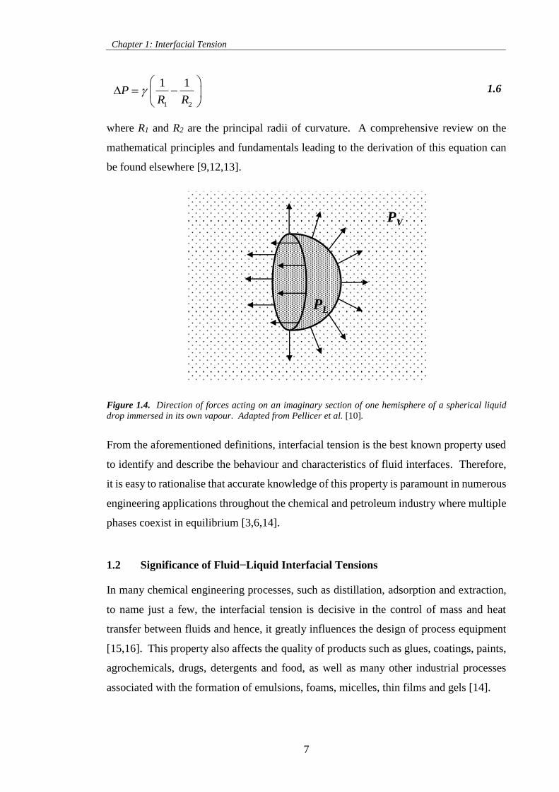
Chapter 1: Interfacial Tension
7
1 2
1 1P
R R
1.6
where R1 and R2 are the principal radii of curvature. A comprehensive review on the
mathematical principles and fundamentals leading to the derivation of this equation can
be found elsewhere [9,12,13].
Figure 1.4. Direction of forces acting on an imaginary section of one hemisphere of a spherical liquid
drop immersed in its own vapour. Adapted from Pellicer et al. [10].
From the aforementioned definitions, interfacial tension is the best known property used
to identify and describe the behaviour and characteristics of fluid interfaces. Therefore,
it is easy to rationalise that accurate knowledge of this property is paramount in numerous
engineering applications throughout the chemical and petroleum industry where multiple
phases coexist in equilibrium [3,6,14].
1.2 Significance of Fluid−Liquid Interfacial Tensions
In many chemical engineering processes, such as distillation, adsorption and extraction,
to name just a few, the interfacial tension is decisive in the control of mass and heat
transfer between fluids and hence, it greatly influences the design of process equipment
[15,16]. This property also affects the quality of products such as glues, coatings, paints,
agrochemicals, drugs, detergents and food, as well as many other industrial processes
associated with the formation of emulsions, foams, micelles, thin films and gels [14].
PL
PV
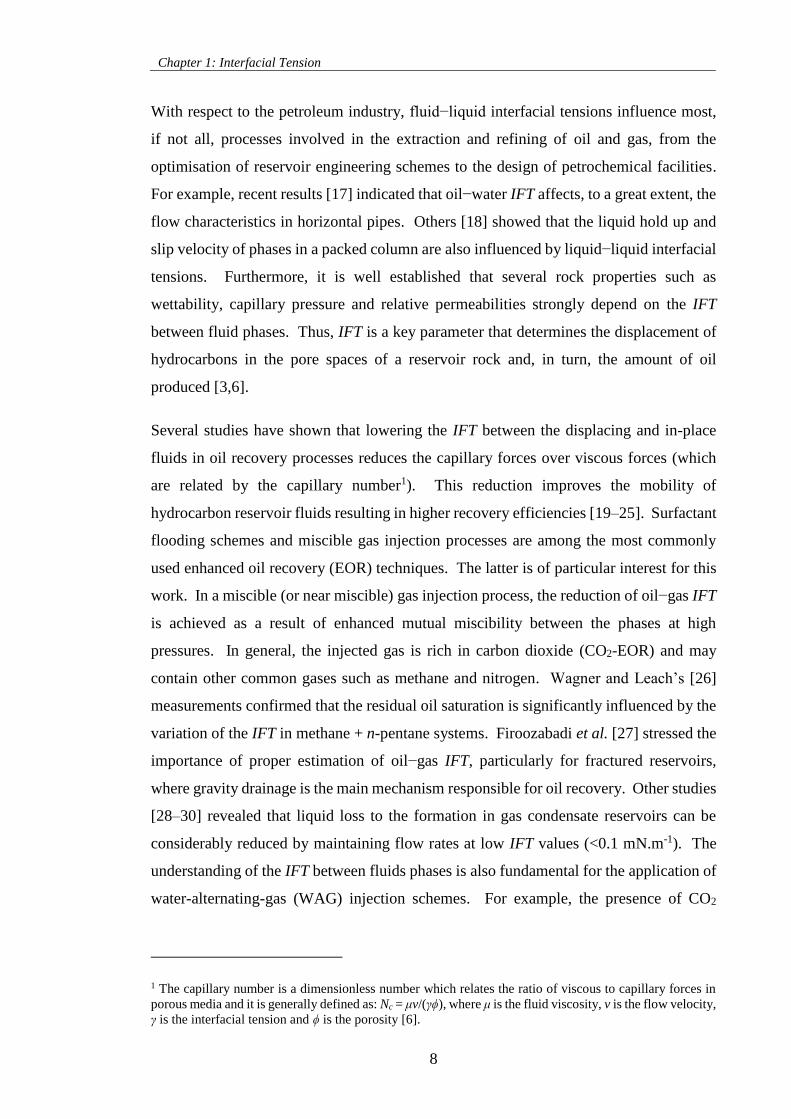
Chapter 1: Interfacial Tension
8
With respect to the petroleum industry, fluid−liquid interfacial tensions influence most,
if not all, processes involved in the extraction and refining of oil and gas, from the
optimisation of reservoir engineering schemes to the design of petrochemical facilities.
For example, recent results [17] indicated that oil−water IFT affects, to a great extent, the
flow characteristics in horizontal pipes. Others [18] showed that the liquid hold up and
slip velocity of phases in a packed column are also influenced by liquid−liquid interfacial
tensions. Furthermore, it is well established that several rock properties such as
wettability, capillary pressure and relative permeabilities strongly depend on the IFT
between fluid phases. Thus, IFT is a key parameter that determines the displacement of
hydrocarbons in the pore spaces of a reservoir rock and, in turn, the amount of oil
produced [3,6].
Several studies have shown that lowering the IFT between the displacing and in-place
fluids in oil recovery processes reduces the capillary forces over viscous forces (which
are related by the capillary number1). This reduction improves the mobility of
hydrocarbon reservoir fluids resulting in higher recovery efficiencies [19–25]. Surfactant
flooding schemes and miscible gas injection processes are among the most commonly
used enhanced oil recovery (EOR) techniques. The latter is of particular interest for this
work. In a miscible (or near miscible) gas injection process, the reduction of oil−gas IFT
is achieved as a result of enhanced mutual miscibility between the phases at high
pressures. In general, the injected gas is rich in carbon dioxide (CO2-EOR) and may
contain other common gases such as methane and nitrogen. Wagner and Leach’s [26]
measurements confirmed that the residual oil saturation is significantly influenced by the
variation of the IFT in methane + n-pentane systems. Firoozabadi et al. [27] stressed the
importance of proper estimation of oil−gas IFT, particularly for fractured reservoirs,
where gravity drainage is the main mechanism responsible for oil recovery. Other studies
[28–30] revealed that liquid loss to the formation in gas condensate reservoirs can be
considerably reduced by maintaining flow rates at low IFT values (<0.1 mN.m-1). The
understanding of the IFT between fluids phases is also fundamental for the application of
water-alternating-gas (WAG) injection schemes. For example, the presence of CO2
1 The capillary number is a dimensionless number which relates the ratio of viscous to capillary forces in
porous media and it is generally defined as: Nc = μv/(γϕ), where μ is the fluid viscosity, v is the flow velocity,
γ is the interfacial tension and ϕ is the porosity [6].
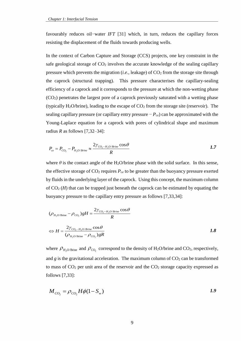
Chapter 1: Interfacial Tension
9
favourably reduces oil−water IFT [31] which, in turn, reduces the capillary forces
resisting the displacement of the fluids towards producing wells.
In the context of Carbon Capture and Storage (CCS) projects, one key constraint in the
safe geological storage of CO2 involves the accurate knowledge of the sealing capillary
pressure which prevents the migration (i.e., leakage) of CO2 from the storage site through
the caprock (structural trapping). This pressure characterises the capillary-sealing
efficiency of a caprock and it corresponds to the pressure at which the non-wetting phase
(CO2) penetrates the largest pore of a caprock previously saturated with a wetting phase
(typically H2O/brine), leading to the escape of CO2 from the storage site (reservoir). The
sealing capillary pressure (or capillary entry pressure − Pce) can be approximated with the
Young-Laplace equation for a caprock with pores of cylindrical shape and maximum
radius R as follows [7,32–34]:
2 2
2 2
/
/
2 cosCO H O Brine
ce CO H O BrineP P PR
1.7
where θ is the contact angle of the H2O/brine phase with the solid surface. In this sense,
the effective storage of CO2 requires Pce to be greater than the buoyancy pressure exerted
by fluids in the underlying layer of the caprock. Using this concept, the maximum column
of CO2 (H) that can be trapped just beneath the caprock can be estimated by equating the
buoyancy pressure to the capillary entry pressure as follows [7,33,34]:
2 2
2 2
/
/Brine
2 cos( )
CO H O Brine
H O CO gHR
2 2
2 2
/
/Brine
2 cos
( )
CO H O Brine
H O CO
HgR
1.8
where 2 /BrineH O and
2CO correspond to the density of H2O/brine and CO2, respectively,
and g is the gravitational acceleration. The maximum column of CO2 can be transformed
to mass of CO2 per unit area of the reservoir and the CO2 storage capacity expressed as
follows [7,33]:
2 2(1 )CO CO wM H S 1.9
Chapter 1: Interfacial Tension
10
where 2COM is the mass of CO2 per unit of surface area of the reservoir, ϕ is the porosity
and Sw is the residual water saturation in the reservoir. From previous definitions it
becomes clear that CO2−H2O/brine IFT is a key parameter in the capillary-sealing
efficiency of a caprock and, consequently, in the CO2 storage capacity by structural
trapping. In the same way, oil−water and oil−gas interfacial tensions are crucial for a
proper estimation of oil and gas reserves [35,36].
Capillary forces are also responsible for the trapping of injected CO2 in the pore spaces
of reservoir rocks such as aquifers. When injected, CO2 will displace the formation fluids
through connected paths in the pore network of a reservoir rock. However, the existence
of a finite CO2−fluid (water/brine) interfacial tension means that CO2 bubbles will remain
immobilized when the formation is reimbibed with the water/brine. This mechanism is
known as capillary or residual trapping and it can account for trapping saturations ranging
from 10 to 30 % of the pore volume of the rock at the end of reimbibition, depending on
the initial CO2 saturation and the reservoir rock properties [37]. It is also important to
note that other mechanisms responsible for the sequestration of CO2 in underground
formations are solubility and mineral trapping [2]. However, these mechanisms operate
in the long-term (from hundreds to millions of years) and their contribution in the short-
term (decades), namely during the injection period, is expected to be small [38].
Among possible geological sites, deep saline aquifers offer the largest CO2 capacity [39];
however, the need for considerable investment in infrastructures have turned depleted
hydrocarbon reservoirs in more attractive alternatives. These reservoirs have an
established geological database and the experience acquired during the oil and gas
exploitation as well as infrastructures already in-place (pipelines, well and surface
equipment) strengthens their potential use as CO2 storage sites [39,40]. Depleted
hydrocarbon reservoirs are filled with connate fluids, constituted of residual gas, oil,
water and ions in solution, and are located in general at depths greater than 800 m, where
temperatures and pressures normally exceed the critical conditions of pure CO2 (Tc ~ 304
K and Pc ~ 7.38 MPa).
All aspects considered, accurate estimation of the effect of pressure, temperature and
composition on the IFT of fluid phases is indispensable for the design and/or optimisation
of not only production and recovery processes of petroleum technology, but also for the
safe and efficient geological storage of CO2.
Chapter 1: Interfacial Tension
11
1.3 Literature Survey
Due to its key role in the design and optimisation of the processes mentioned in the
foregoing section, the study of interfacial tension of both simple and complex mixtures
has been subject of extensive research for many years. Several authors have focused on
measuring fundamental IFT data of binary systems which, in turn, are necessary for the
development and validation of thermodynamic models. A case to point out is the study
of Weinaug and Katz [41] who investigated the interfacial tension of methane + propane
mixtures with the capillary rise technique at temperatures up to 363.2 K and pressures
ranging from 10.34 MPa down to ambient, with measured IFT values ranging from 12.13
down to 0.50 mN.m-1. Through validation with measured data, Weinaug and Katz [41]
heuristically extended to mixtures the equation originally proposed by Macleod [42] and
Sugden [43] for pure substances. This equation is known as the Parachor method and is
still to date widely used in commercial PVT software packages and reservoir simulators
for predicting the interfacial tension between oil and gas phases (CHAPTER 3). A brief
review of IFT data available in literature for systems of interest is now presented.
1.3.1 Hydrocarbon systems
High pressure IFT binary data between n-alkanes and common gases such as carbon
dioxide, methane and nitrogen have been collected for this work. Sources as well as
temperature and pressure conditions are listed in Tables 1.1, 1.2 and 1.3. From these it
can be seen that most studies have been conducted for systems containing n-alkanes with
a carbon number ≤ 10 and over a limited range of temperatures and pressures.
Furthermore, as will be emphasised throughout this work, the measurement of
fluid−liquid interfacial tensions through indirect techniques requires an accurate
estimation of the density of the equilibrated phases in contact. Nourozieh et al. [44]
showed that experimental saturated density data of the CO2 + n-decane system are still
scarce, with most studies limited to measurements of the saturated liquid phase and a
temperature of 344 K. The most wide-ranging study was reported by Reamer and Sage
[45] who measured the volumetric properties of this system at temperatures over the range
278 to 511 K and pressures up to 69 MPa. Nagarajan and Robinson [46], Shaver et al.
[47] and Mejía et al. [48] have also reported saturated phase densities of this system at
temperatures up to 377 K and pressures up to near the critical point. Saturated density
data of n-decane with either CH4 or N2 are also, to the author’s knowledge, still limited
to the works of Sage and co-workers [49,50], Amin and Smith [51] and Jianhua et al.
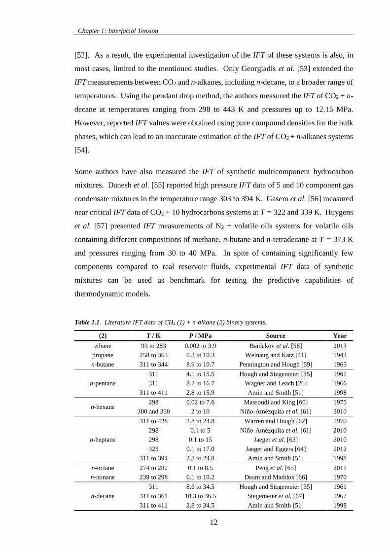
Chapter 1: Interfacial Tension
12
[52]. As a result, the experimental investigation of the IFT of these systems is also, in
most cases, limited to the mentioned studies. Only Georgiadis et al. [53] extended the
IFT measurements between CO2 and n-alkanes, including n-decane, to a broader range of
temperatures. Using the pendant drop method, the authors measured the IFT of CO2 + n-
decane at temperatures ranging from 298 to 443 K and pressures up to 12.15 MPa.
However, reported IFT values were obtained using pure compound densities for the bulk
phases, which can lead to an inaccurate estimation of the IFT of CO2 + n-alkanes systems
[54].
Some authors have also measured the IFT of synthetic multicomponent hydrocarbon
mixtures. Danesh et al. [55] reported high pressure IFT data of 5 and 10 component gas
condensate mixtures in the temperature range 303 to 394 K. Gasem et al. [56] measured
near critical IFT data of CO2 + 10 hydrocarbons systems at T = 322 and 339 K. Huygens
et al. [57] presented IFT measurements of N2 + volatile oils systems for volatile oils
containing different compositions of methane, n-butane and n-tetradecane at T = 373 K
and pressures ranging from 30 to 40 MPa. In spite of containing significantly few
components compared to real reservoir fluids, experimental IFT data of synthetic
mixtures can be used as benchmark for testing the predictive capabilities of
thermodynamic models.
Table 1.1. Literature IFT data of CH4 (1) + n-alkane (2) binary systems.
(2) T / K P / MPa Source Year
ethane 93 to 283 0.002 to 3.9 Baidakov et al. [58] 2013
propane 258 to 363 0.3 to 10.3 Weinaug and Katz [41] 1943
n-butane 311 to 344 8.9 to 10.7 Pennington and Hough [59] 1965
n-pentane
311 4.1 to 15.5 Hough and Stegemeier [35] 1961
311 8.2 to 16.7 Wagner and Leach [26] 1966
311 to 411 2.8 to 15.9 Amin and Smith [51] 1998
n-hexane 298 0.02 to 7.6 Massoudi and King [60] 1975
300 and 350 2 to 10 Niño-Amézquita et al. [61] 2010
n-heptane
311 to 428 2.8 to 24.8 Warren and Hough [62] 1970
298 0.1 to 5 Niño-Amézquita et al. [61] 2010
298 0.1 to 15 Jaeger et al. [63] 2010
323 0.1 to 17.0 Jaeger and Eggers [64] 2012
311 to 394 2.8 to 24.8 Amin and Smith [51] 1998
n-octane 274 to 282 0.1 to 8.5 Peng et al. [65] 2011
n-nonane 239 to 298 0.1 to 10.2 Deam and Maddox [66] 1970
n-decane
311 8.6 to 34.5 Hough and Stegemeier [35] 1961
311 to 361 10.3 to 36.5 Stegemeier et al. [67] 1962
311 to 411 2.8 to 34.5 Amin and Smith [51] 1998
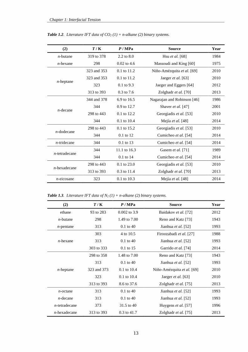
Chapter 1: Interfacial Tension
13
Table 1.2. Literature IFT data of CO2 (1) + n-alkane (2) binary systems.
(2) T / K P / MPa Source Year
n-butane 319 to 378 2.2 to 8.0 Hsu et al. [68] 1984
n-hexane 298 0.02 to 4.6 Massoudi and King [60] 1975
n-heptane
323 and 353 0.1 to 11.2 Niño-Amézquita et al. [69] 2010
323 and 353 0.1 to 11.2 Jaeger et al. [63] 2010
323 0.1 to 9.3 Jaeger and Eggers [64] 2012
313 to 393 0.3 to 7.6 Zolghadr et al. [70] 2013
n-decane
344 and 378 6.9 to 16.5 Nagarajan and Robinson [46] 1986
344 0.9 to 12.7 Shaver et al. [47] 2001
298 to 443 0.1 to 12.2 Georgiadis et al. [53] 2010
344 0.1 to 10.4 Mejía et al. [48] 2014
n-dodecane 298 to 443 0.1 to 15.2 Georgiadis et al. [53] 2010
344 0.1 to 12 Cumicheo et al. [54] 2014
n-tridecane 344 0.1 to 13 Cumicheo et al. [54] 2014
n-tetradecane 344 11.1 to 16.3 Gasem et al. [71] 1989
344 0.1 to 14 Cumicheo et al. [54] 2014
n-hexadecane 298 to 443 0.1 to 23.0 Georgiadis et al. [53] 2010
313 to 393 0.3 to 11.4 Zolghadr et al. [70] 2013
n-eicosane 323 0.1 to 10.3 Mejía et al. [48] 2014
Table 1.3. Literature IFT data of N2 (1) + n-alkane (2) binary systems.
(2) T / K P / MPa Source Year
ethane 93 to 283 0.002 to 3.9 Baidakov et al. [72] 2012
n-butane 298 1.49 to 7.00 Reno and Katz [73] 1943
n-pentane 313 0.1 to 40 Jianhua et al. [52] 1993
n-hexane
303 4 to 10.5 Firoozabadi et al. [27] 1988
313 0.1 to 40 Jianhua et al. [52] 1993
303 to 333 0.1 to 15 Garrido et al. [74] 2014
n-heptane
298 to 358 1.48 to 7.00 Reno and Katz [73] 1943
313 0.1 to 40 Jianhua et al. [52] 1993
323 and 373 0.1 to 10.4 Niño-Amézquita et al. [69] 2010
323 0.1 to 10.4 Jaeger et al. [63] 2010
313 to 393 8.6 to 37.6 Zolghadr et al. [75] 2013
n-octane 313 0.1 to 40 Jianhua et al. [52] 1993
n-decane 313 0.1 to 40 Jianhua et al. [52] 1993
n-tetradecane 373 31.5 to 40 Huygens et al. [57] 1996
n-hexadecane 313 to 393 0.3 to 41.7 Zolghadr et al. [75] 2013
Chapter 1: Interfacial Tension
14
1.3.2 Aqueous systems
The interfacial properties of aqueous systems have attracted a great attention from
researchers during the past two decades due to its influence in many different technical
areas. Considering its importance on the geological storage of CO2, many studies have
been conducted on the experimental measurement of the IFT of the CO2 + H2O system
[7,76–94]. In most of these studies the pendant drop method has been used to measure
CO2−H2O IFTs over a wide range of experimental conditions. However, at the time of
this work and to the author’s knowledge, data available in literature above 398 K are still
limited to the study of Shariat et al. [93].
A brief literature review carried by Georgiadis et al. [91] showed that CO2−H2O IFT data
above CO2 supercritical conditions are scarce and/or inconsistent. Amongst all factors
pointed for these discrepancies, the assumption of pure density for the phases involved
and the presence of impurities stand out as the most important factors. Yaginuma et al.
[95], Hebach et al. [96], Kvamme et al. [87], Chiquet et al. [7], Bachu and Bennion [89],
Tabasinejad et al. [97], Shariat et al. [93] and, more recently, Efika et al. [98], measured
densities of the saturated phases with a vibrating U-tube densitometer. Their results
showed that the approximation of the water-saturated CO2-rich phase density to that of
pure CO2 [99] is in fact valid for temperatures and pressures up to 473 K and 140 MPa,
respectively. However, as demonstrated by Chiquet et al. [7], the effect of dissolved CO2
on the density of the liquid aqueous phase can cause severe underestimation of the IFTs
close to the density inversion conditions, where the deviations of the real (measured)
density difference from that of pure substances are greatest. For systems with relatively
low mutual solubility such as hydrocarbon + water and nitrogen + water, the density of
the saturated phases has been commonly approximated to that of pure substances [100–
104] without any significant loss of accuracy. The second factor is the most difficult to
control. Impurities are inherently present in trace amounts in any high pressure setup and
can behave as surfactants decreasing the interfacial tension values [81,83,84,86]. Thus,
a thorough cleaning procedure of the experimental device with different solvents is
recommended before measuring this property. All things considered, the experimental
studies on CO2−H2O IFT considered in this work are listed in Table 1.4.
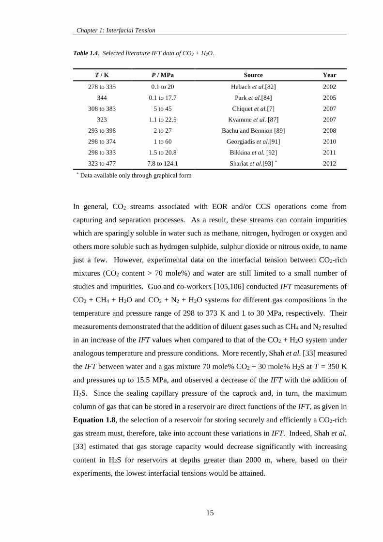
Chapter 1: Interfacial Tension
15
Table 1.4. Selected literature IFT data of CO2 + H2O.
T / K P / MPa Source Year
278 to 335 0.1 to 20 Hebach et al.[82] 2002
344 0.1 to 17.7 Park et al.[84] 2005
308 to 383 5 to 45 Chiquet et al.[7] 2007
323 1.1 to 22.5 Kvamme et al. [87] 2007
293 to 398 2 to 27 Bachu and Bennion [89] 2008
298 to 374 1 to 60 Georgiadis et al.[91] 2010
298 to 333 1.5 to 20.8 Bikkina et al. [92] 2011
323 to 477 7.8 to 124.1 Shariat et al.[93] * 2012
* Data available only through graphical form
In general, CO2 streams associated with EOR and/or CCS operations come from
capturing and separation processes. As a result, these streams can contain impurities
which are sparingly soluble in water such as methane, nitrogen, hydrogen or oxygen and
others more soluble such as hydrogen sulphide, sulphur dioxide or nitrous oxide, to name
just a few. However, experimental data on the interfacial tension between CO2-rich
mixtures (CO2 content > 70 mole%) and water are still limited to a small number of
studies and impurities. Guo and co-workers [105,106] conducted IFT measurements of
CO2 + CH4 + H2O and CO2 + N2 + H2O systems for different gas compositions in the
temperature and pressure range of 298 to 373 K and 1 to 30 MPa, respectively. Their
measurements demonstrated that the addition of diluent gases such as CH4 and N2 resulted
in an increase of the IFT values when compared to that of the CO2 + H2O system under
analogous temperature and pressure conditions. More recently, Shah et al. [33] measured
the IFT between water and a gas mixture 70 mole% CO2 + 30 mole% H2S at T = 350 K
and pressures up to 15.5 MPa, and observed a decrease of the IFT with the addition of
H2S. Since the sealing capillary pressure of the caprock and, in turn, the maximum
column of gas that can be stored in a reservoir are direct functions of the IFT, as given in
Equation 1.8, the selection of a reservoir for storing securely and efficiently a CO2-rich
gas stream must, therefore, take into account these variations in IFT. Indeed, Shah et al.
[33] estimated that gas storage capacity would decrease significantly with increasing
content in H2S for reservoirs at depths greater than 2000 m, where, based on their
experiments, the lowest interfacial tensions would be attained.
Chapter 1: Interfacial Tension
16
The presence of dissolved ions in the formation water is also an important aspect that
should be taken into account. Cations such as Na+, K+ Ca2+, Mg2+ and anions such as Cl-,
SO4- and HCO3
-, to name just a few, are among the most abundant ions in the reservoir
brine; the total concentration of these ions typically increases with reservoir depth and
can reach concentrations of up to or greater than 400 g.L-1 [89].
It is well established that the addition of salts such as NaCl, KCl, CaCl2 or MgCl2, affects
the physical properties and phase behaviour of aqueous systems, in particular the IFT.
Several authors [90,107–113] have related the increase of gas−water IFT upon the
addition of salts to the distribution of ions between the interfacial region and the bulk
aqueous phase. Johansson and Eriksson [108] reported surface tension values for
different salt solutions that exceeded those of salt-free water under analogous conditions.
Using the concept of an electrolyte free layer and Gibbs adsorption equation, the authors
[108] showed that the IFT increase must be related to the negative adsorption (i.e.,
depletion) of ions in the interface and, thereby to their tendency to remain in the aqueous
bulk phase. Hey et al. [114] showed that in 1:1 electrolytes solutions this increase was
directly proportional to the enthalpy of hydration of ions (i.e., attraction to water),
suggesting that ions were preferably fully hydrated in the bulk aqueous phase than partly
hydrated in the interface. In general, the attraction of cations to water molecules is
stronger than anions and hence, cations are strongly repelled while anions approach more
closely to the interface [108,113]. Such gradient of ions results in an electrostatic
potential differential at the interface which enhances the offset of water molecules from
the interface towards the aqueous bulk phase and increases the magnitude of the
interfacial tension [115]. Cation hydration increases as the ratio of cation charge to cation
surface area is increased and thus the impact on the IFT is expected to increase as follows
[116]:
2 2
4Cs Rb NH K Na Li Ca Mg 1.10
The findings described above are in agreement with Molecular Dynamics simulations
performed by Li et al. [117] for CO2 + brine systems and salts with the chloride (Cl-)
anion over a broad range of pressure and temperature conditions. In their work, computed
IFT values and density profiles of species across the interface also indicated a negative
adsorption (negative surface excess) of ions at the interface.
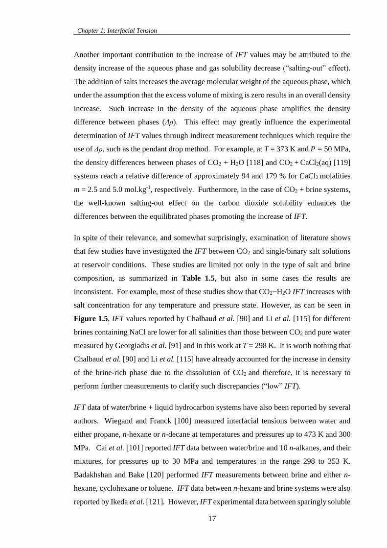
Chapter 1: Interfacial Tension
17
Another important contribution to the increase of IFT values may be attributed to the
density increase of the aqueous phase and gas solubility decrease (“salting-out” effect).
The addition of salts increases the average molecular weight of the aqueous phase, which
under the assumption that the excess volume of mixing is zero results in an overall density
increase. Such increase in the density of the aqueous phase amplifies the density
difference between phases (Δρ). This effect may greatly influence the experimental
determination of IFT values through indirect measurement techniques which require the
use of Δρ, such as the pendant drop method. For example, at T = 373 K and P = 50 MPa,
the density differences between phases of CO2 + H2O [118] and CO2 + CaCl2(aq) [119]
systems reach a relative difference of approximately 94 and 179 % for CaCl2 molalities
m = 2.5 and 5.0 mol.kg-1, respectively. Furthermore, in the case of CO2 + brine systems,
the well-known salting-out effect on the carbon dioxide solubility enhances the
differences between the equilibrated phases promoting the increase of IFT.
In spite of their relevance, and somewhat surprisingly, examination of literature shows
that few studies have investigated the IFT between CO2 and single/binary salt solutions
at reservoir conditions. These studies are limited not only in the type of salt and brine
composition, as summarized in Table 1.5, but also in some cases the results are
inconsistent. For example, most of these studies show that CO2−H2O IFT increases with
salt concentration for any temperature and pressure state. However, as can be seen in
Figure 1.5, IFT values reported by Chalbaud et al. [90] and Li et al. [115] for different
brines containing NaCl are lower for all salinities than those between CO2 and pure water
measured by Georgiadis et al. [91] and in this work at T = 298 K. It is worth nothing that
Chalbaud et al. [90] and Li et al. [115] have already accounted for the increase in density
of the brine-rich phase due to the dissolution of CO2 and therefore, it is necessary to
perform further measurements to clarify such discrepancies (“low” IFT).
IFT data of water/brine + liquid hydrocarbon systems have also been reported by several
authors. Wiegand and Franck [100] measured interfacial tensions between water and
either propane, n-hexane or n-decane at temperatures and pressures up to 473 K and 300
MPa. Cai et al. [101] reported IFT data between water/brine and 10 n-alkanes, and their
mixtures, for pressures up to 30 MPa and temperatures in the range 298 to 353 K.
Badakhshan and Bake [120] performed IFT measurements between brine and either n-
hexane, cyclohexane or toluene. IFT data between n-hexane and brine systems were also
reported by Ikeda et al. [121]. However, IFT experimental data between sparingly soluble
Chapter 1: Interfacial Tension
18
gases and brine at reservoir conditions are scarce in literature and, to the author’s
knowledge, still limited to the IFT of brine + natural gas [122] and brine + methane
systems [103].
Of relevance for the scope of this work are also the works of Jennings and Newman [123]
and Georgiadis et al. [31] as well as studies previously conducted in our laboratories
[124]. Jennings and Newman [123] and Georgiadis et al. [31] reported two-phase IFT
data of the CH4 + n-decane + H2O and CO2 + n-decane + H2O systems, respectively.
Therein, the authors investigated the impact of CH4/CO2 composition in the single
hydrocarbon phase on the interfacial tension with water. The required density difference
data were estimated by Jennings and Newman [123] based on density measurements of
the mutually saturated phases whereas Georgiadis et al. [31] used pure H2O density for
the water-rich phase and modelled densities for the n-decane-rich phase. On the other
hand, volumetric and IFT data of four water + hydrocarbon mixtures were measured in
our laboratories in the context of a reservoir fluid studies project (2002−2005) [124], and
the results reported through the works of Bahramian et al. [125] and Pereira et al. [126].
The systems investigated included three ternary mixtures CH4 + n-decane + H2O, CH4 +
n-hexadecane + H2O and CH4 + toluene + H2O, and a quaternary mixture CH4 + n-decane
+ cyclohexane + H2O. Two- and three-phase interfacial tensions were measured at T =
423 K and over a wide range of equilibrium pressures (up to 140 MPa). IFT
measurements were made between water-rich liquid and equilibrium vapour phase,
hydrocarbon-rich liquid and equilibrium vapour phase, and water-rich liquid and
hydrocarbon-rich liquid. Together, these studies provide valuable insights on the IFT
between phases that coexist in the pore spaces of reservoir rocks and simulate, to some
extent, IFTs variations during EOR and CO2 storage processes due to changes in
composition, temperature and pressure.
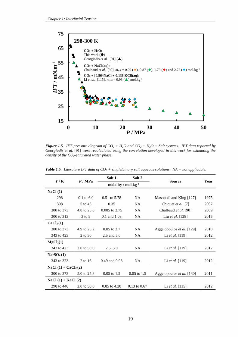
Chapter 1: Interfacial Tension
19
Figure 1.5. IFT-pressure diagram of CO2 + H2O and CO2 + H2O + Salt systems. IFT data reported by
Georgiadis et al. [91] were recalculated using the correlation developed in this work for estimating the
density of the CO2-saturated water phase.
Table 1.5. Literature IFT data of CO2 + single/binary salt aqueous solutions. NA = not applicable.
T / K P / MPa Salt 1 Salt 2
Source Year molality / mol.kg-1
NaCl (1)
298 0.1 to 6.0 0.51 to 5.78 NA Massoudi and King [127] 1975
308 5 to 45 0.35 NA Chiquet et al. [7] 2007
300 to 373 4.8 to 25.8 0.085 to 2.75 NA Chalbaud et al. [90] 2009
300 to 313 3 to 9 0.1 and 1.03 NA Liu et al. [128] 2015
CaCl2 (1)
300 to 373 4.9 to 25.2 0.05 to 2.7 NA Aggelopoulos et al. [129] 2010
343 to 423 2 to 50 2.5 and 5.0 NA Li et al. [119] 2012
MgCl2(1)
343 to 423 2.0 to 50.0 2.5, 5.0 NA Li et al. [119] 2012
Na2SO4 (1)
343 to 373 2 to 16 0.49 and 0.98 NA Li et al. [119] 2012
NaCl (1) + CaCl2 (2)
300 to 373 5.0 to 25.3 0.05 to 1.5 0.05 to 1.5 Aggelopoulos et al. [130] 2011
NaCl (1) + KaCl (2)
298 to 448 2.0 to 50.0 0.85 to 4.28 0.13 to 0.67 Li et al. [115] 2012
15
25
35
45
55
65
75
0 10 20 30 40 50
IFT
/ m
N.m
-1
P / MPa
298-300 K
CO2 + H2O:
This work ()
Georgiadis et al. [91] ()
CO2 + NaCl(aq):
Chalbaud et al. [90], msalt = 0.09 (), 0.87 (), 1.79 () and 2.75 () mol.kg-1
CO2 + [0.864NaCl + 0.136 KCl](aq):
Li et al. [115], msalt = 0.98 () mol.kg-1

Chapter 1: Interfacial Tension
20
1.4 Summary
The interpretation of interfacial tension has been explained along with the concepts of
wettability, contact angle and capillary pressure. From these it was possible to show that
fluid−liquid interfacial tensions play a key role in many practical applications where
multiple phases coexist in equilibrium. Particular attention was given to the impact of
IFTs on the saturation, distribution and displacement of hydrocarbon and aqueous phases
in a reservoir as well as on the geological storage of CO2.
A critical analysis has also been performed on experimental IFT data available in
literature for binary and multicomponent systems comprising reservoir fluids. The impact
of density, diluent gases and salts on the IFT were briefly discussed. The systems which
require further investigation were identified: gas + n-decane (gas = CO2, CH4 and N2) and
carbon dioxide + water/brine.
21
CHAPTER 2 – EXPERIMENTAL TECHNIQUES FOR
MEASURING INTERFACIAL TENSION
2.1 Introduction
Due to its major role in many technical areas, a number of tensiometers have been
developed for the experimental determination of the IFT between fluid phases in contact.
Among all 17 techniques reviewed by Dorsey [131] in 1926, only a few are still
commonly employed for interfacial tension measurements in fluid−liquid interfaces. The
most popular techniques are depicted schematically in Figure 2.1. They were briefly
reviewed in 2002 by Drelich et al. [132] and are described in detail in Rusanov and
Prokhorov’s book [11]. The Pendant Drop (PD) and Capillary Rise (CR) methods, due
to their simplicity and ease of implementation at high pressure and high temperature
(HPHT) conditions, are arguably the most widely used methods for measuring the IFT of
reservoir fluids.
In the context of the PD technique, a drop of a denser fluid is formed at the tip of a
capillary tube and kept in equilibrium with a surrounding less dense fluid (vapour or
liquid) and the shape of the drop is subsequently analysed, as depicted in Figure 2.1f. On
the other hand, the CR method relies on the fundamentals of capillarity and on the rise of
fluids in capillary tubes as depicted in Figure 2.1e. Once the profile of the drop or the
height of the liquid column are determined, they are combined with pertinent phase
density data to obtain interfacial tension values. In essence, the estimation of the IFT
with the foregoing techniques relies on the balance between capillary and gravity forces.
In the CR method the IFT forces are balanced with a variable volume of liquid, whereas
in the PD drop the effect of gravity on the shape of a drop of fixed volume is analysed
[132].
The accurate measurement of IFT with the PD method requires a sufficiently large density
difference between the phases to elongate the drop, reducing the errors that arise from the
determination of the profile of the drop. For this reason, the CR technique is in general
preferred for systems at/or near critical conditions, where the density difference and the
IFT values are considerably lower. Overall, these methods have been applied in the study
of interfacial phenomena of a variety of fluids and interfaces over a broad range of
conditions and with established high precision and repeatability [11].
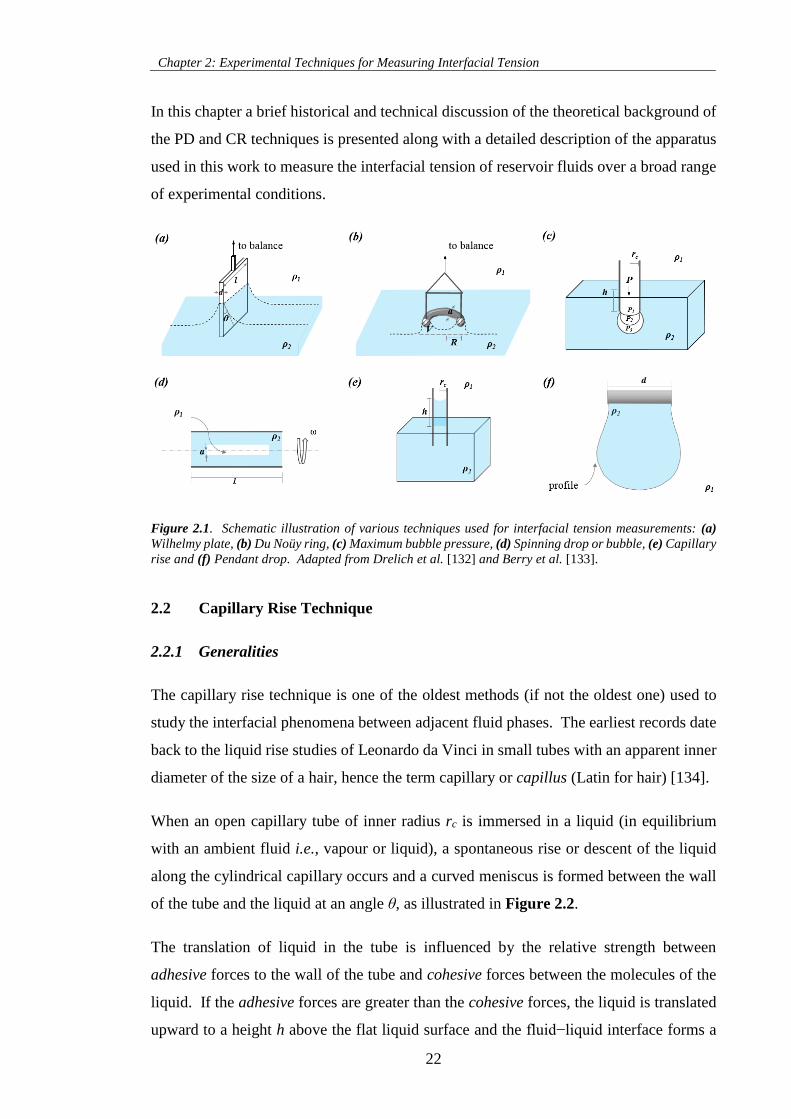
Chapter 2: Experimental Techniques for Measuring Interfacial Tension
22
In this chapter a brief historical and technical discussion of the theoretical background of
the PD and CR techniques is presented along with a detailed description of the apparatus
used in this work to measure the interfacial tension of reservoir fluids over a broad range
of experimental conditions.
Figure 2.1. Schematic illustration of various techniques used for interfacial tension measurements: (a)
Wilhelmy plate, (b) Du Noüy ring, (c) Maximum bubble pressure, (d) Spinning drop or bubble, (e) Capillary
rise and (f) Pendant drop. Adapted from Drelich et al. [132] and Berry et al. [133].
2.2 Capillary Rise Technique
2.2.1 Generalities
The capillary rise technique is one of the oldest methods (if not the oldest one) used to
study the interfacial phenomena between adjacent fluid phases. The earliest records date
back to the liquid rise studies of Leonardo da Vinci in small tubes with an apparent inner
diameter of the size of a hair, hence the term capillary or capillus (Latin for hair) [134].
When an open capillary tube of inner radius rc is immersed in a liquid (in equilibrium
with an ambient fluid i.e., vapour or liquid), a spontaneous rise or descent of the liquid
along the cylindrical capillary occurs and a curved meniscus is formed between the wall
of the tube and the liquid at an angle θ, as illustrated in Figure 2.2.
The translation of liquid in the tube is influenced by the relative strength between
adhesive forces to the wall of the tube and cohesive forces between the molecules of the
liquid. If the adhesive forces are greater than the cohesive forces, the liquid is translated
upward to a height h above the flat liquid surface and the fluid−liquid interface forms a
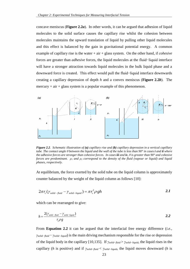
Chapter 2: Experimental Techniques for Measuring Interfacial Tension
23
concave meniscus (Figure 2.2a). In other words, it can be argued that adhesion of liquid
molecules to the solid surface causes the capillary rise whilst the cohesion between
molecules maintains the upward translation of liquid by pulling other liquid molecules
and this effect is balanced by the gain in gravitational potential energy. A common
example of capillary rise is the water + air + glass system. On the other hand, if cohesive
forces are greater than adhesive forces, the liquid molecules at the fluid−liquid interface
will have a stronger attraction towards liquid molecules in the bulk liquid phase and a
downward force is created. This effect would pull the fluid−liquid interface downwards
creating a capillary depression of depth h and a convex meniscus (Figure 2.2b). The
mercury + air + glass system is a popular example of this phenomenon.
Figure 2.2. Schematic illustration of (a) capillary rise and (b) capillary depression in a vertical capillary
tube. The contact angle θ between the liquid and the wall of the tube is less than 90° in cases i and ii where
the adhesive forces are stronger than cohesive forces. In cases iii and iv, θ is greater than 90° and cohesive
forces are predominant. ρ1 and ρ2 correspond to the density of the fluid (vapour or liquid) and liquid
phases, respectively.
At equilibrium, the force exerted by the solid tube on the liquid column is approximately
counter balanced by the weight of the liquid column as follows [10]:
22 ( )c solid fluid solid liquid cr r gh 2.1
which can be rearranged to give:
2( )solid fluid solid liquid
c
hr g
2.2
From Equation 2.2 it can be argued that the interfacial free energy difference (i.e.,
γsolid−fluid − γsolid−liquid) is the main driving mechanism responsible for the rise or depression
of the liquid body in the capillary [10,135]. If γsolid−fluid > γsolid−liquid, the liquid rises in the
capillary (h is positive) and if γsolid−fluid < γsolid−liquid, the liquid moves downward (h is
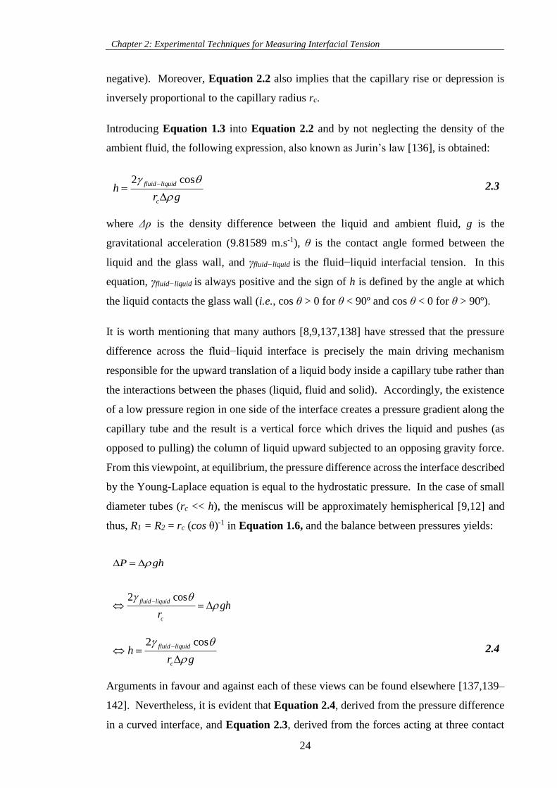
Chapter 2: Experimental Techniques for Measuring Interfacial Tension
24
negative). Moreover, Equation 2.2 also implies that the capillary rise or depression is
inversely proportional to the capillary radius rc.
Introducing Equation 1.3 into Equation 2.2 and by not neglecting the density of the
ambient fluid, the following expression, also known as Jurin’s law [136], is obtained:
2 cosfluid liquid
c
hr g
2.3
where Δρ is the density difference between the liquid and ambient fluid, g is the
gravitational acceleration (9.81589 m.s-1), θ is the contact angle formed between the
liquid and the glass wall, and γfluid−liquid is the fluid−liquid interfacial tension. In this
equation, γfluid−liquid is always positive and the sign of h is defined by the angle at which
the liquid contacts the glass wall (i.e., cos θ > 0 for θ < 90º and cos θ < 0 for θ > 90º).
It is worth mentioning that many authors [8,9,137,138] have stressed that the pressure
difference across the fluid−liquid interface is precisely the main driving mechanism
responsible for the upward translation of a liquid body inside a capillary tube rather than
the interactions between the phases (liquid, fluid and solid). Accordingly, the existence
of a low pressure region in one side of the interface creates a pressure gradient along the
capillary tube and the result is a vertical force which drives the liquid and pushes (as
opposed to pulling) the column of liquid upward subjected to an opposing gravity force.
From this viewpoint, at equilibrium, the pressure difference across the interface described
by the Young-Laplace equation is equal to the hydrostatic pressure. In the case of small
diameter tubes (rc << h), the meniscus will be approximately hemispherical [9,12] and
thus, R1 = R2 = rc (cos θ)-1 in Equation 1.6, and the balance between pressures yields:
P gh
2 cosfluid liquid
c
ghr
2 cosfluid liquid
c
hr g
2.4
Arguments in favour and against each of these views can be found elsewhere [137,139–
142]. Nevertheless, it is evident that Equation 2.4, derived from the pressure difference
in a curved interface, and Equation 2.3, derived from the forces acting at three contact
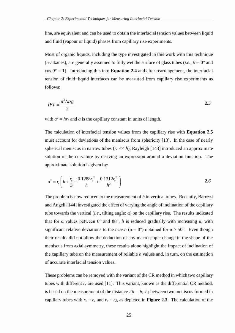
Chapter 2: Experimental Techniques for Measuring Interfacial Tension
25
line, are equivalent and can be used to obtain the interfacial tension values between liquid
and fluid (vapour or liquid) phases from capillary rise experiments.
Most of organic liquids, including the type investigated in this work with this technique
(n-alkanes), are generally assumed to fully wet the surface of glass tubes (i.e., θ = 0° and
cos 0° = 1). Introducing this into Equation 2.4 and after rearrangement, the interfacial
tension of fluid−liquid interfaces can be measured from capillary rise experiments as
follows:
2
2
a gIFT
2.5
with a2 = hrc and a is the capillary constant in units of length.
The calculation of interfacial tension values from the capillary rise with Equation 2.5
must account for deviations of the meniscus from sphericity [13]. In the case of nearly
spherical meniscus in narrow tubes (rc << h), Rayleigh [143] introduced an approximate
solution of the curvature by deriving an expression around a deviation function. The
approximate solution is given by:
2 32
2
0.1288 0.1312
3
c c cc
r r ra r h
h h
2.6
The problem is now reduced to the measurement of h in vertical tubes. Recently, Barozzi
and Angeli [144] investigated the effect of varying the angle of inclination of the capillary
tube towards the vertical (i.e., tilting angle: α) on the capillary rise. The results indicated
that for α values between 0° and 88°, h is reduced gradually with increasing α, with
significant relative deviations to the true h (α = 0°) obtained for α > 50°. Even though
their results did not allow the deduction of any macroscopic change in the shape of the
meniscus from axial symmetry, these results alone highlight the impact of inclination of
the capillary tube on the measurement of reliable h values and, in turn, on the estimation
of accurate interfacial tension values.
These problems can be removed with the variant of the CR method in which two capillary
tubes with different rc are used [11]. This variant, known as the differential CR method,
is based on the measurement of the distance Δh = h1-h2 between two meniscus formed in
capillary tubes with rc = r1 and rc = r2, as depicted in Figure 2.3. The calculation of the
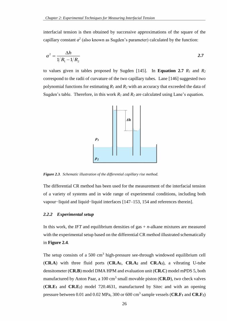
Chapter 2: Experimental Techniques for Measuring Interfacial Tension
26
interfacial tension is then obtained by successive approximations of the square of the
capillary constant a2 (also known as Sugden’s parameter) calculated by the function:
2
1 21 1
ha
R R
2.7
to values given in tables proposed by Sugden [145]. In Equation 2.7 R1 and R2
correspond to the radii of curvature of the two capillary tubes. Lane [146] suggested two
polynomial functions for estimating R1 and R2 with an accuracy that exceeded the data of
Sugden’s table. Therefore, in this work R1 and R2 are calculated using Lane’s equation.
Figure 2.3. Schematic illustration of the differential capillary rise method.
The differential CR method has been used for the measurement of the interfacial tension
of a variety of systems and in wide range of experimental conditions, including both
vapour−liquid and liquid−liquid interfaces [147–153, 154 and references therein].
2.2.2 Experimental setup
In this work, the IFT and equilibrium densities of gas + n-alkane mixtures are measured
with the experimental setup based on the differential CR method illustrated schematically
in Figure 2.4.
The setup consists of a 500 cm3 high-pressure see-through windowed equilibrium cell
(CR.A) with three fluid ports (CR.A1, CR.A2 and CR.A3), a vibrating U-tube
densitometer (CR.B) model DMA HPM and evaluation unit (CR.C) model mPDS 5, both
manufactured by Anton Paar, a 100 cm3 small movable piston (CR.D), two check valves
(CR.E1 and CR.E2) model 720.4631, manufactured by Sitec and with an opening
pressure between 0.01 and 0.02 MPa, 300 or 600 cm3 sample vessels (CR.F1 and CR.F2)
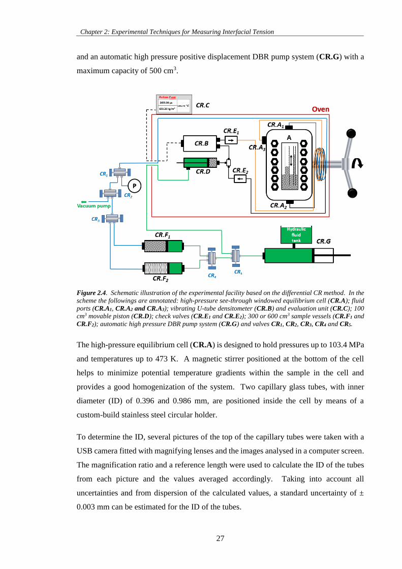
Chapter 2: Experimental Techniques for Measuring Interfacial Tension
27
and an automatic high pressure positive displacement DBR pump system (CR.G) with a
maximum capacity of 500 cm3.
Figure 2.4. Schematic illustration of the experimental facility based on the differential CR method. In the
scheme the followings are annotated: high-pressure see-through windowed equilibrium cell (CR.A); fluid
ports (CR.A1, CR.A2 and CR.A3); vibrating U-tube densitometer (CR.B) and evaluation unit (CR.C); 100
cm3 movable piston (CR.D); check valves (CR.E1 and CR.E2); 300 or 600 cm3 sample vessels (CR.F1 and
CR.F2); automatic high pressure DBR pump system (CR.G) and valves CR1, CR2, CR3, CR4 and CR5.
The high-pressure equilibrium cell (CR.A) is designed to hold pressures up to 103.4 MPa
and temperatures up to 473 K. A magnetic stirrer positioned at the bottom of the cell
helps to minimize potential temperature gradients within the sample in the cell and
provides a good homogenization of the system. Two capillary glass tubes, with inner
diameter (ID) of 0.396 and 0.986 mm, are positioned inside the cell by means of a
custom-build stainless steel circular holder.
To determine the ID, several pictures of the top of the capillary tubes were taken with a
USB camera fitted with magnifying lenses and the images analysed in a computer screen.
The magnification ratio and a reference length were used to calculate the ID of the tubes
from each picture and the values averaged accordingly. Taking into account all
uncertainties and from dispersion of the calculated values, a standard uncertainty of ±
0.003 mm can be estimated for the ID of the tubes.
Chapter 2: Experimental Techniques for Measuring Interfacial Tension
28
The fluid ports CR.A2 and CR.A3 of the cell are connected to the inlet and outlet of the
densitometer (CR.B) by means of 0.29 mm ID high-pressure tubing with measured length
of 3 m which ensures a minimum volume of approximately 0.2 cm3. The two check
valves (CR.E1 and CR.E2) and the movable piston (CR.D) enables a closed loop flow of
fluids between the equilibrium cell and the densitometer. Turning the equilibrium cell
upside down allows the density measurement of either the saturated liquid or vapour
phase. All parts described before are housed inside an oven, manufactured by Cincinnati
Sub-Zero model Z-16, with an overall temperature control stability of ± 0.1 K.
The pressure is monitored by means of a pressure transducer (Quartzdyne Series I)
connected to valve CR1 and previously calibrated against a dead weight pressure balance.
This calibration procedure ensures a standard uncertainty of u(P) = 0.04 MPa. The
temperature is measured by a high precision built-in thermometer in the densitometer
with a specified standard uncertainty of u(T) = 0.1 K. The temperature readings from the
densitometer were checked against a Prema 3040 high precision thermometer and
deviations were observed to be within the densitometer uncertainties.
Tested fluids are stored in sample vessels and loaded into equilibrium cell through valves
CR1, CR2 and CR3 and fluid port CR.A1. Each sample vessel contains a piston which
can be used to control the internal volume of the vessel and, consequently, the pressure.
The back pressure in both the sample vessels (CR.F1 and CR.F2) and the movable piston
(CR.D) are controlled by means of pressurized hydraulic fluid and the DBR pump system
(CR.G), and also valves CR4 and CR5.
An image capturing system (not shown in Figure 2.4) is used to measure the height of
the liquid rise in the capillaries. It consists of a camera (Cohu model DSP 3600) mounted
in a structure capable of vertical displacement (cathetometer). High magnification lenses
are fitted into the camera and images, with a magnification factor higher than 15x, are
displayed in a computer screen. As an example, a picture taken with this setup is depicted
in Figure 2.5.
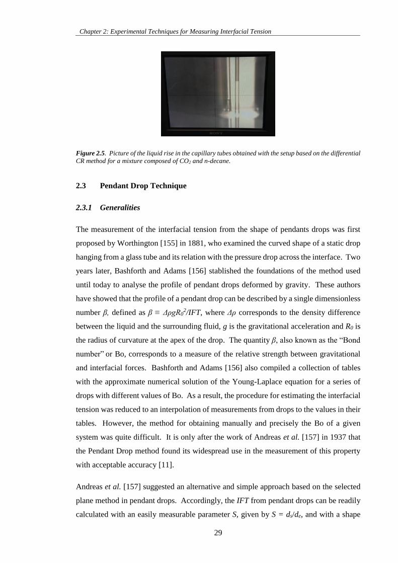
Chapter 2: Experimental Techniques for Measuring Interfacial Tension
29
Figure 2.5. Picture of the liquid rise in the capillary tubes obtained with the setup based on the differential
CR method for a mixture composed of CO2 and n-decane.
2.3 Pendant Drop Technique
2.3.1 Generalities
The measurement of the interfacial tension from the shape of pendants drops was first
proposed by Worthington [155] in 1881, who examined the curved shape of a static drop
hanging from a glass tube and its relation with the pressure drop across the interface. Two
years later, Bashforth and Adams [156] stablished the foundations of the method used
until today to analyse the profile of pendant drops deformed by gravity. These authors
have showed that the profile of a pendant drop can be described by a single dimensionless
number β, defined as β ≡ ΔρgR02/IFT, where Δρ corresponds to the density difference
between the liquid and the surrounding fluid, g is the gravitational acceleration and R0 is
the radius of curvature at the apex of the drop. The quantity β, also known as the “Bond
number” or Bo, corresponds to a measure of the relative strength between gravitational
and interfacial forces. Bashforth and Adams [156] also compiled a collection of tables
with the approximate numerical solution of the Young-Laplace equation for a series of
drops with different values of Bo. As a result, the procedure for estimating the interfacial
tension was reduced to an interpolation of measurements from drops to the values in their
tables. However, the method for obtaining manually and precisely the Bo of a given
system was quite difficult. It is only after the work of Andreas et al. [157] in 1937 that
the Pendant Drop method found its widespread use in the measurement of this property
with acceptable accuracy [11].
Andreas et al. [157] suggested an alternative and simple approach based on the selected
plane method in pendant drops. Accordingly, the IFT from pendant drops can be readily
calculated with an easily measurable parameter S, given by S = ds/de, and with a shape
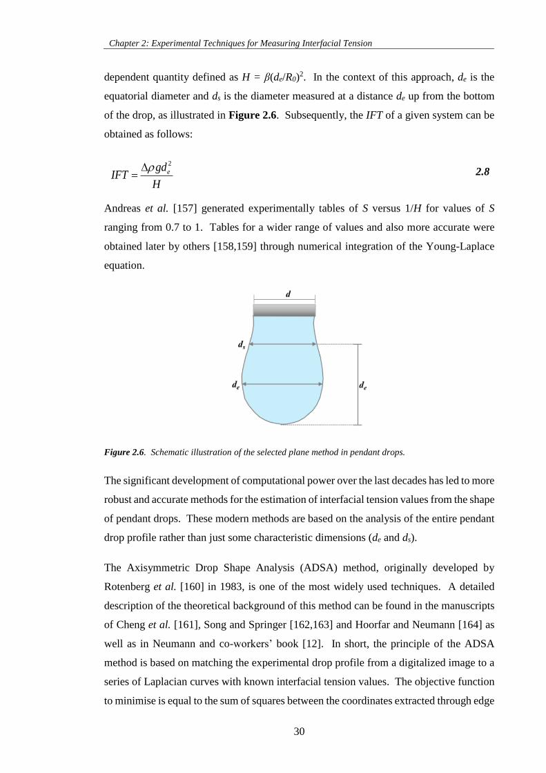
Chapter 2: Experimental Techniques for Measuring Interfacial Tension
30
dependent quantity defined as H = β(de/R0)2. In the context of this approach, de is the
equatorial diameter and ds is the diameter measured at a distance de up from the bottom
of the drop, as illustrated in Figure 2.6. Subsequently, the IFT of a given system can be
obtained as follows:
2
egdIFT
H
2.8
Andreas et al. [157] generated experimentally tables of S versus 1/H for values of S
ranging from 0.7 to 1. Tables for a wider range of values and also more accurate were
obtained later by others [158,159] through numerical integration of the Young-Laplace
equation.
Figure 2.6. Schematic illustration of the selected plane method in pendant drops.
The significant development of computational power over the last decades has led to more
robust and accurate methods for the estimation of interfacial tension values from the shape
of pendant drops. These modern methods are based on the analysis of the entire pendant
drop profile rather than just some characteristic dimensions (de and ds).
The Axisymmetric Drop Shape Analysis (ADSA) method, originally developed by
Rotenberg et al. [160] in 1983, is one of the most widely used techniques. A detailed
description of the theoretical background of this method can be found in the manuscripts
of Cheng et al. [161], Song and Springer [162,163] and Hoorfar and Neumann [164] as
well as in Neumann and co-workers’ book [12]. In short, the principle of the ADSA
method is based on matching the experimental drop profile from a digitalized image to a
series of Laplacian curves with known interfacial tension values. The objective function
to minimise is equal to the sum of squares between the coordinates extracted through edge
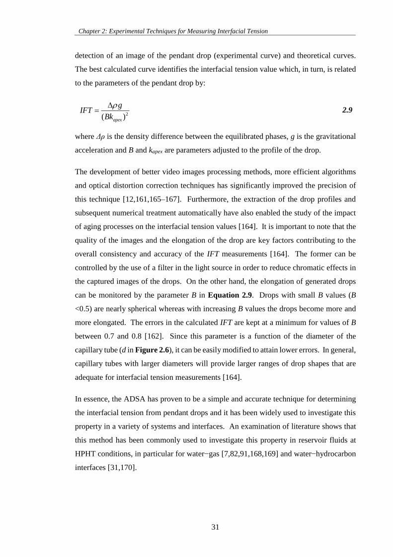
Chapter 2: Experimental Techniques for Measuring Interfacial Tension
31
detection of an image of the pendant drop (experimental curve) and theoretical curves.
The best calculated curve identifies the interfacial tension value which, in turn, is related
to the parameters of the pendant drop by:
2( )apex
gIFT
Bk
2.9
where Δρ is the density difference between the equilibrated phases, g is the gravitational
acceleration and B and kapex are parameters adjusted to the profile of the drop.
The development of better video images processing methods, more efficient algorithms
and optical distortion correction techniques has significantly improved the precision of
this technique [12,161,165–167]. Furthermore, the extraction of the drop profiles and
subsequent numerical treatment automatically have also enabled the study of the impact
of aging processes on the interfacial tension values [164]. It is important to note that the
quality of the images and the elongation of the drop are key factors contributing to the
overall consistency and accuracy of the IFT measurements [164]. The former can be
controlled by the use of a filter in the light source in order to reduce chromatic effects in
the captured images of the drops. On the other hand, the elongation of generated drops
can be monitored by the parameter B in Equation 2.9. Drops with small B values (B
<0.5) are nearly spherical whereas with increasing B values the drops become more and
more elongated. The errors in the calculated IFT are kept at a minimum for values of B
between 0.7 and 0.8 [162]. Since this parameter is a function of the diameter of the
capillary tube (d in Figure 2.6), it can be easily modified to attain lower errors. In general,
capillary tubes with larger diameters will provide larger ranges of drop shapes that are
adequate for interfacial tension measurements [164].
In essence, the ADSA has proven to be a simple and accurate technique for determining
the interfacial tension from pendant drops and it has been widely used to investigate this
property in a variety of systems and interfaces. An examination of literature shows that
this method has been commonly used to investigate this property in reservoir fluids at
HPHT conditions, in particular for water−gas [7,82,91,168,169] and water−hydrocarbon
interfaces [31,170].
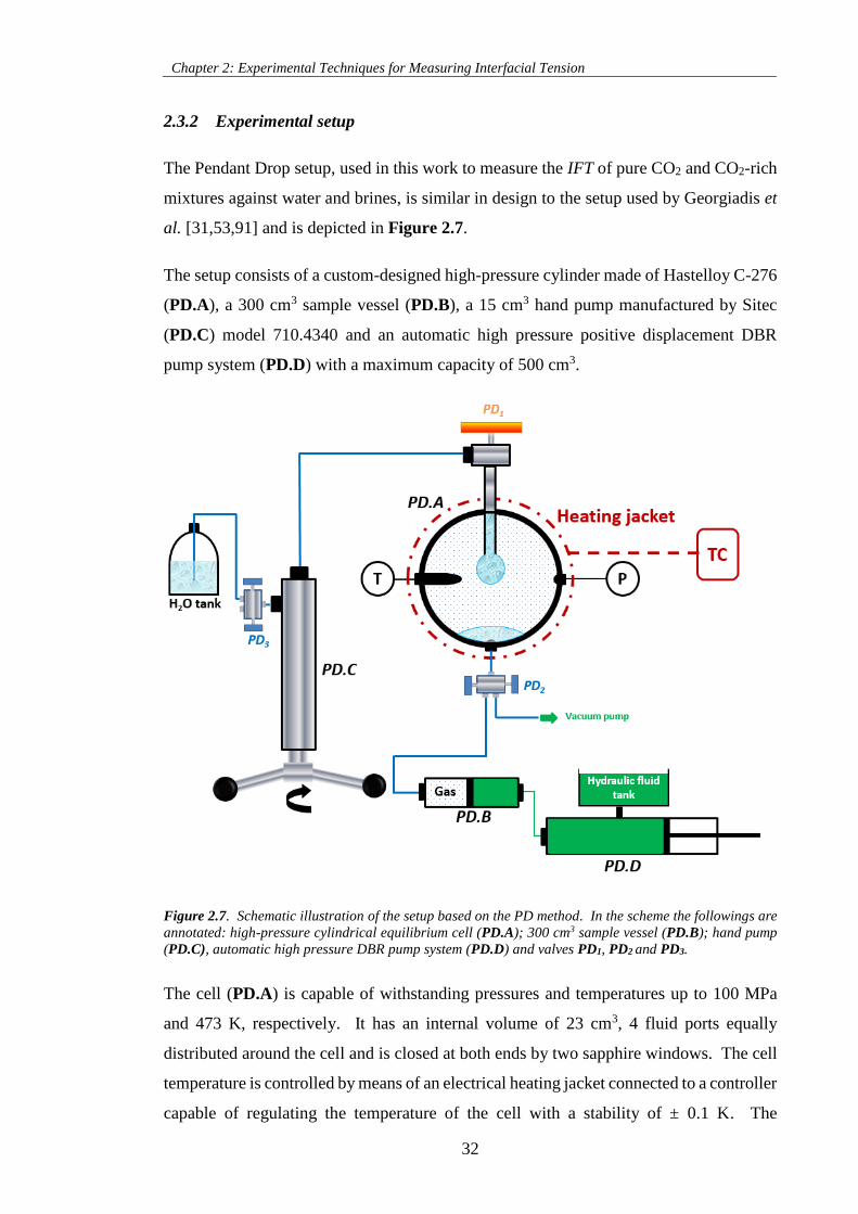
Chapter 2: Experimental Techniques for Measuring Interfacial Tension
32
2.3.2 Experimental setup
The Pendant Drop setup, used in this work to measure the IFT of pure CO2 and CO2-rich
mixtures against water and brines, is similar in design to the setup used by Georgiadis et
al. [31,53,91] and is depicted in Figure 2.7.
The setup consists of a custom-designed high-pressure cylinder made of Hastelloy C-276
(PD.A), a 300 cm3 sample vessel (PD.B), a 15 cm3 hand pump manufactured by Sitec
(PD.C) model 710.4340 and an automatic high pressure positive displacement DBR
pump system (PD.D) with a maximum capacity of 500 cm3.
Figure 2.7. Schematic illustration of the setup based on the PD method. In the scheme the followings are
annotated: high-pressure cylindrical equilibrium cell (PD.A); 300 cm3 sample vessel (PD.B); hand pump
(PD.C), automatic high pressure DBR pump system (PD.D) and valves PD1, PD2 and PD3.
The cell (PD.A) is capable of withstanding pressures and temperatures up to 100 MPa
and 473 K, respectively. It has an internal volume of 23 cm3, 4 fluid ports equally
distributed around the cell and is closed at both ends by two sapphire windows. The cell
temperature is controlled by means of an electrical heating jacket connected to a controller
capable of regulating the temperature of the cell with a stability of ± 0.1 K. The
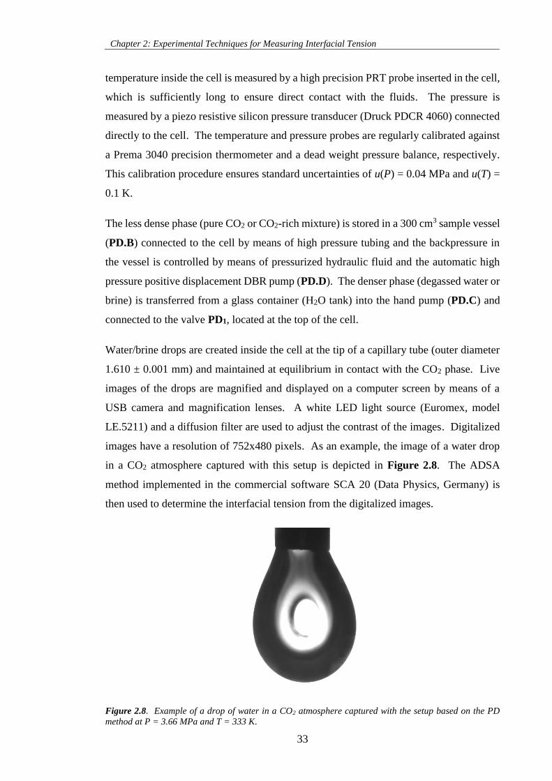
Chapter 2: Experimental Techniques for Measuring Interfacial Tension
33
temperature inside the cell is measured by a high precision PRT probe inserted in the cell,
which is sufficiently long to ensure direct contact with the fluids. The pressure is
measured by a piezo resistive silicon pressure transducer (Druck PDCR 4060) connected
directly to the cell. The temperature and pressure probes are regularly calibrated against
a Prema 3040 precision thermometer and a dead weight pressure balance, respectively.
This calibration procedure ensures standard uncertainties of u(P) = 0.04 MPa and u(T) =
0.1 K.
The less dense phase (pure CO2 or CO2-rich mixture) is stored in a 300 cm3 sample vessel
(PD.B) connected to the cell by means of high pressure tubing and the backpressure in
the vessel is controlled by means of pressurized hydraulic fluid and the automatic high
pressure positive displacement DBR pump (PD.D). The denser phase (degassed water or
brine) is transferred from a glass container (H2O tank) into the hand pump (PD.C) and
connected to the valve PD1, located at the top of the cell.
Water/brine drops are created inside the cell at the tip of a capillary tube (outer diameter
1.610 ± 0.001 mm) and maintained at equilibrium in contact with the CO2 phase. Live
images of the drops are magnified and displayed on a computer screen by means of a
USB camera and magnification lenses. A white LED light source (Euromex, model
LE.5211) and a diffusion filter are used to adjust the contrast of the images. Digitalized
images have a resolution of 752x480 pixels. As an example, the image of a water drop
in a CO2 atmosphere captured with this setup is depicted in Figure 2.8. The ADSA
method implemented in the commercial software SCA 20 (Data Physics, Germany) is
then used to determine the interfacial tension from the digitalized images.
Figure 2.8. Example of a drop of water in a CO2 atmosphere captured with the setup based on the PD
method at P = 3.66 MPa and T = 333 K.
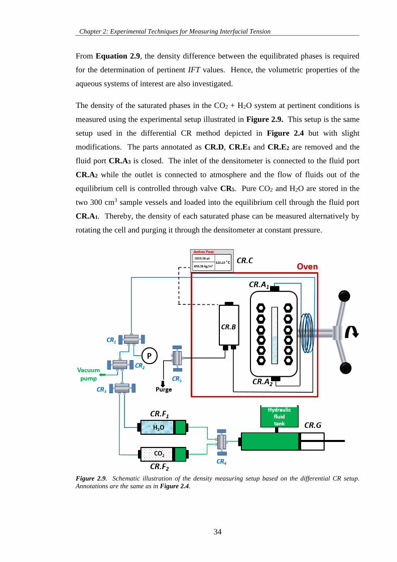
Chapter 2: Experimental Techniques for Measuring Interfacial Tension
34
From Equation 2.9, the density difference between the equilibrated phases is required
for the determination of pertinent IFT values. Hence, the volumetric properties of the
aqueous systems of interest are also investigated.
The density of the saturated phases in the CO2 + H2O system at pertinent conditions is
measured using the experimental setup illustrated in Figure 2.9. This setup is the same
setup used in the differential CR method depicted in Figure 2.4 but with slight
modifications. The parts annotated as CR.D, CR.E1 and CR.E2 are removed and the
fluid port CR.A3 is closed. The inlet of the densitometer is connected to the fluid port
CR.A2 while the outlet is connected to atmosphere and the flow of fluids out of the
equilibrium cell is controlled through valve CR5. Pure CO2 and H2O are stored in the
two 300 cm3 sample vessels and loaded into the equilibrium cell through the fluid port
CR.A1. Thereby, the density of each saturated phase can be measured alternatively by
rotating the cell and purging it through the densitometer at constant pressure.
Figure 2.9. Schematic illustration of the density measuring setup based on the differential CR setup.
Annotations are the same as in Figure 2.4.
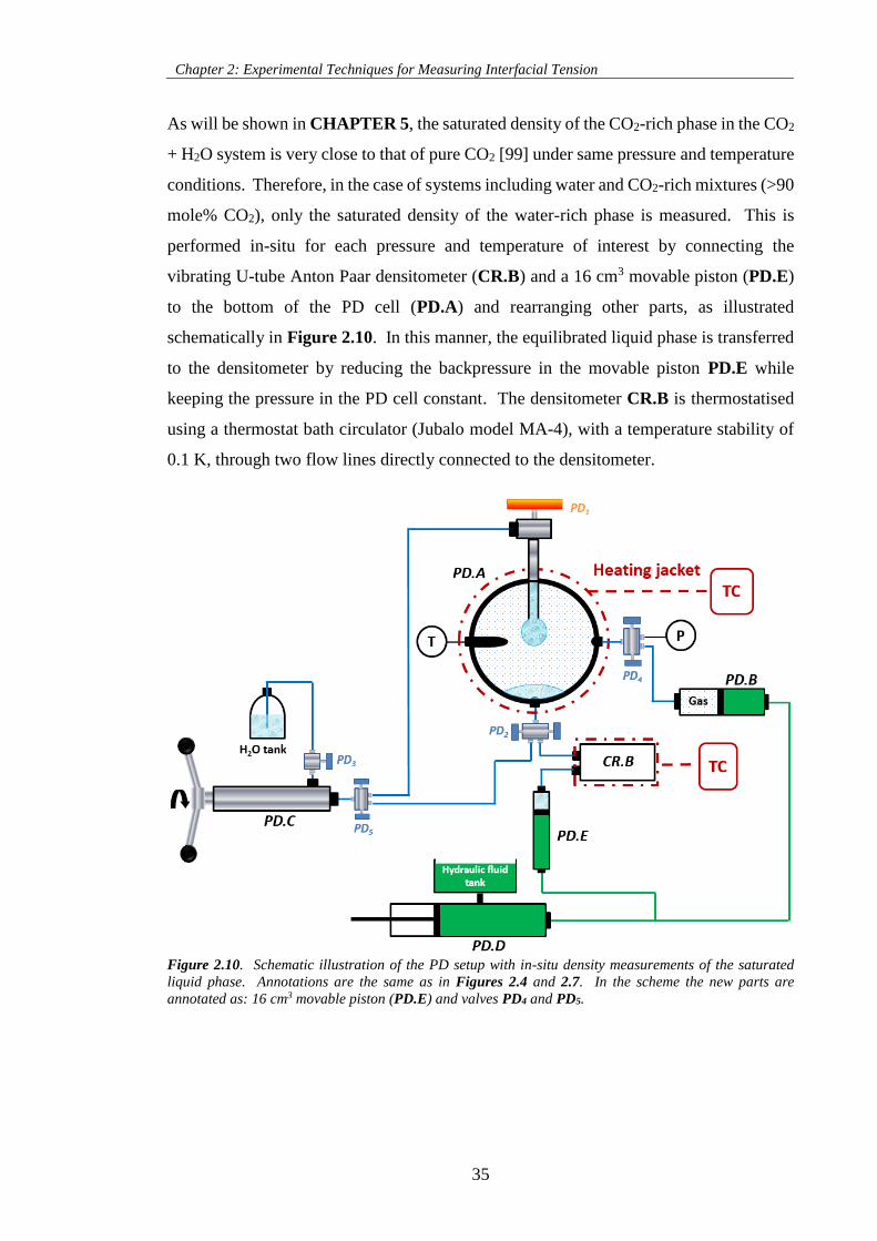
Chapter 2: Experimental Techniques for Measuring Interfacial Tension
35
As will be shown in CHAPTER 5, the saturated density of the CO2-rich phase in the CO2
+ H2O system is very close to that of pure CO2 [99] under same pressure and temperature
conditions. Therefore, in the case of systems including water and CO2-rich mixtures (>90
mole% CO2), only the saturated density of the water-rich phase is measured. This is
performed in-situ for each pressure and temperature of interest by connecting the
vibrating U-tube Anton Paar densitometer (CR.B) and a 16 cm3 movable piston (PD.E)
to the bottom of the PD cell (PD.A) and rearranging other parts, as illustrated
schematically in Figure 2.10. In this manner, the equilibrated liquid phase is transferred
to the densitometer by reducing the backpressure in the movable piston PD.E while
keeping the pressure in the PD cell constant. The densitometer CR.B is thermostatised
using a thermostat bath circulator (Jubalo model MA-4), with a temperature stability of
0.1 K, through two flow lines directly connected to the densitometer.
Figure 2.10. Schematic illustration of the PD setup with in-situ density measurements of the saturated
liquid phase. Annotations are the same as in Figures 2.4 and 2.7. In the scheme the new parts are
annotated as: 16 cm3 movable piston (PD.E) and valves PD4 and PD5.

Chapter 2: Experimental Techniques for Measuring Interfacial Tension
36
2.4 Summary
Two experimental setups and their theoretical background for measuring the IFT of
fluid−liquid interfaces have been described. The experimental setups are based on the
differential capillary rise (CR) and pendant drop (PD) techniques. The first is suitable for
measuring this property in systems at/or near critical conditions where low values are
expected (IFT < 1.5 mN.m-1). Hence, the CR setup is used in CHAPTER 4 to measure
the IFT of synthetic hydrocarbon reservoir fluids. The IFT between aqueous and
CO2-rich phases is measured with the PD setup and the results presented in CHAPTER
5. Aiming at reporting more realistic IFT values, a vibrating U-tube densitometer is also
used to measure saturated density data of the investigated systems.
37
CHAPTER 3 – THERMODYNAMIC MODELLING OF
INTERFACIAL TENSION
3.1 Introduction
The high costs of experimental facilities and the time needed to perform these
measurements necessitate the deployment of theoretical tools, which when validated with
experimental data over a broad range of conditions can be used to correlate or even predict
interfacial tensions.
Numerous approaches have been proposed and many empirical or semi-empirical
methods are being used as standard models in commercial simulators for the Oil and Gas
industry. The most popular approaches include the Parachor method [42,43], scaling law
[171], the corresponding-states theory [172–174], thermodynamic [175,176] and
empirical correlations [116,177,178]. Among these, the Parachor method [41,42] and the
scaling law [171] gained the most attention due to their simplicity and accuracy for
describing the IFT of vapour−liquid interfaces in hydrocarbon systems. Even though a
Parachor value has been reported for water, this method is not recommended for the
prediction of IFT of aqueous interfaces [179,180]. Instead, a more accurate and reliable
model for estimating the interfacial tension of hydrocarbon + water systems was proposed
by Firoozabadi and Ramey [180]. In their work, the authors successfully correlated the
IFT between water and hydrocarbons against the density of the contacted phases over a
broad range of conditions. Later, Argaud [116] and Sutton [177,178] developed new
versions of the original correlation from Firoozabadi and Ramey [180] by readjusting the
model to a broader class of compounds and larger database. Although good results were
obtained with these approaches, they are limited on their transferability and predictive
capabilities.
Other more robust methods, based on statistical thermodynamics, take into account the
molecular distribution of species across the interface. Some of these methods include the
perturbation theory [181], integral and density functional theories [181–184], the Linear
Gradient Theory (LGT) [185,186] and the Square Gradient Theory (SGT) or Density
Gradient Theory (DGT) [187,188]. In particular, the latter has been thoroughly applied
in the prediction of IFT values of a wide class of systems and interfaces. Such systems
include pure substances and mixtures containing hydrocarbons [54,61,69,189–200],
alcohols [189,201–204], esters [205,206], glycols [207], polymers [208–210], near
Chapter 3: Thermodynamic Modelling of Interfacial Tension
38
critical systems [211–214], real petroleum mixtures [196,215] and most recently, aqueous
systems containing common gases such as CO2, CH4 and N2 [168,216–223]. It is worth
mentioning that several authors have also successfully described this property using
Molecular Dynamic (MD) and Monte Carlo (MC) computer simulation approaches
[48,117,197,218,223–233].
The accurate estimation of IFT values with the methods described above relies on a
correct description of both composition and density of the bulk phases by a
thermodynamic phase behaviour model. In general, classical cubic equations of state
(EoSs) such as the Soave-Redlich-Kwong 1972 (SRK72) EoS [234] and the Peng-
Robinson 1978 (PR78) EoS [235] are used for simple systems containing just gases and
hydrocarbons. On the other hand, theoretically sound EoSs are preferred for systems
containing polar and/or associating compounds such as water, alcohols and glycols, with
strong hydrogen bonding interactions. The most popular are the Statistical Associating
Fluid Theory (SAFT) [236–238] EoS, and its variants, and the Cubic-Plus-Association
(CPA) [239,240] EoS.
In this chapter a brief description of the theoretical approaches used to describe the phase
behaviour and IFT of reservoir fluids is presented. Aiming at searching for one accurate
and general model for predicting the IFT of multiphase systems containing both
associating and non-associating molecules, the predictive capabilities of the DGT
[187,188] are further assessed in this work by comparison with experimental IFT data as
well as with other theoretical approaches such as the Parachor [42,43], Sutton’s
correlation [178] and the LGT [185,186].
3.2 Parachor Method
The Parachor model [42,43] and its derivatives are indeed the most successful and widely
used approaches in the petroleum industry due to their simplicity and good description of
the IFT of both simple and complex reservoir mixtures at HPHT conditions. In the
Parachor approach, the interfacial tension can be correlated to the bulk density difference
of the phases in equilibrium by the equation proposed by Macleod [42] and Sugden [43]
for pure substances:
Chapter 3: Thermodynamic Modelling of Interfacial Tension
39
1/ ( )E L V
chIFT P 3.1
where Pch is the Parachor value, ρL and ρV are the liquid and vapour molar density of the
coexisting saturated phases and E is the scaling exponent. The scaling exponent
characterises the dependence of IFT with the density difference as the latter quantity
vanishes near the critical point.
Using the simple molar averaging technique, Weinaug and Katz [41] extended this
approach to mixtures:
1/E
,
1
(x )compN
L V
ch i i i
i
IFT P y
3.2
where xi and yi are the equilibrium mole fractions of component i in the liquid and vapour
phases, respectively, and Pch,i is the Parachor of component i.
A considerable volume of research and review works show in detail modifications for the
scaling exponent, with values ranging from 3.45 to 4, and correlations for expressing the
Parachor values as function of properties such as molecular weight and specific gravity
or critical properties. Reviewed modifications can be found in the work of Ali [241] as
well as of Daniel et al. [242]. In this work, E is set equal to 4 and the Parachor values of
well-defined substances, in units of (mN.m-1)1/4.(g.cm-3)-1, are calculated with the
correlation regressed by Fanchi [243]:
2 3
, 0 1 , 2 , 3 4 5 6 /ch i c i c i i i i iP a aV a T a H a H a H a H 3.3
5/6 1/4
, ,i c i c iH V T 3.4
where Tc,i and Vc,i are the critical temperature (K) and the critical volume (L.mol-1) of
component i, respectively. Regressed coefficients a0 to a6 are listed in Table 3.1. This
correlation can be used to calculate the Parachor of n-alkanes up to C20 as well as of
common gases such as CO2, N2 and CH4. In the case of real petroleum fluids, several
researches [27,243–245] have recognized that the Parachor of the heaviest fraction (or
residue of distillation) exhibits a discontinuity from the other distillation cuts apparently
due to the presence of heavy surface active compounds of asphaltic nature. As an attempt
to circumvent this problem, and as a way of estimating the Parachor of cuts, Fanchi [243]
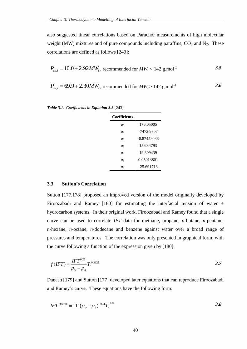
Chapter 3: Thermodynamic Modelling of Interfacial Tension
40
also suggested linear correlations based on Parachor measurements of high molecular
weight (MW) mixtures and of pure compounds including paraffins, CO2 and N2. These
correlations are defined as follows [243]:
, 10.0 2.92ch i iP MW , recommended for MWi < 142 g.mol-1 3.5
, 69.9 2.30ch i iP MW , recommended for MWi > 142 g.mol-1 3.6
Table 3.1. Coefficients in Equation 3.3 [243].
Coefficients
a0 176.05005
a1 -7472.9807
a2 -0.87458088
a3 1560.4793
a4 19.309439
a5 0.05013801
a6 -25.691718
3.3 Sutton’s Correlation
Sutton [177,178] proposed an improved version of the model originally developed by
Firoozabadi and Ramey [180] for estimating the interfacial tension of water +
hydrocarbon systems. In their original work, Firoozabadi and Ramey found that a single
curve can be used to correlate IFT data for methane, propane, n-butane, n-pentane,
n-hexane, n-octane, n-dodecane and benzene against water over a broad range of
pressures and temperatures. The correlation was only presented in graphical form, with
the curve following a function of the expression given by [180]:
0.250.3125( ) r
w h
IFTf IFT T
3.7
Danesh [179] and Sutton [177] developed later equations that can reproduce Firoozabadi
and Ramey’s curve. These equations have the following form:
1.251.024111( )Danesh
w h rIFT T
3.8
Chapter 3: Thermodynamic Modelling of Interfacial Tension
41
4
0.3125
1.58( ) 1.76Sutton w h
r
IFTT
3.9
In 2009, Sutton [178] improved the accuracy of his earlier version of the correlation by
replacing the exponent 0.3125 with a quadratic function of temperature and readjusting
the remaining constants in Equation 3.9 to a larger database. Data sources comprised
IFT data used in the original work of Firoozabadi and Ramey [180] as well as more
recently published IFT data between water and various pure hydrocarbon compounds,
including methane through n-hexadecane, toluene and benzene. In order to accurately
describe the effect of temperature, Sutton [178] also included in the analysis pure water
IFT data at saturation conditions (i.e, surface tension). Supplement IFT data of
multicomponent gas mixtures against water were also used to test the model. The
improved correlation has the following form [178]:
3 6 2
3.6667
(0.821976 1.83785 10 1.34016 10 )
1.53988( ) 2.08339w h
T T
r
IFTT
3.10
where ρw and ρh are the density of the water and hydrocarbon phases in g.cm-3,
respectively, T is the temperature of the system in units of R° and Tr is the reduced
temperature of the hydrocarbon phase, defined as Tr = Tc/T. The critical temperature Tc
takes the value of 302.881 for gas−water interfacial tension calculations.
In his approach, Sutton [178] considered the density of the hydrocarbon and water phases
to be approximately equal to that of pure compounds determined from multi-parameter
models. Therefore, the accuracy of this correlation in predicting IFT values can be rather
affected by changes from pure density values due to the mutual dissolution of water and
hydrocarbons molecules, in particular the increase of water molecules in the oleic phase
at high temperatures. Nevertheless, the new model represented in Equation 3.10 allowed
a description of the IFT of gas + water and liquid hydrocarbon + water binary mixtures
over a wide range of pressure and temperature conditions, with calculated deviations
significantly lower than those obtained with Equations 3.8 and 3.9. Also, the good
results obtained for the interfacial tension between water and gas mixtures including up
to 40 mole% CO2 or up to 49 mole% N2, showed the potential of the improved model for
describing more realistic systems.
Chapter 3: Thermodynamic Modelling of Interfacial Tension
42
3.4 Density Gradient Theory
The Density Gradient Theory (DGT) of fluid interfaces is a more rigorous theoretical
approach which has gradually shown to be a good tool for predicting interfacial
properties. This theory has its origins in the work of van der Waals [246], but only after
the reformulation of Cahn and Hilliard [187] it was found useful in modelling interfacial
properties. Accordingly, the DGT approach considers the free energy density of
homogeneous fluid (bulk phase) and the influence parameter of inhomogeneous fluid
(interface) to determine the density gradient of components across the interface by
minimization of the Helmholtz free energy and to compute interfacial tension values. In
general, EoSs are used to estimate the equilibrium properties of the bulk phases and to
evaluate the energy across the interface. The influence parameters, although they can be
derived from theoretical expressions [199,212,247], are usually fitted against surface
tension data of pure substances. Since the DGT has already been presented in great detail
by several authors in literature, the reader is referred to the studies of Miqueu et al.
[191,192,194], Davis’ book [248], Carey’s [249] and Cornelisse’s thesis [250] for a
comprehensive description of the model; a brief description is now presented.
3.4.1 Theory outline
The basis of the DGT lies on the gradient theory formulated in 1894 by van der Waals
[246]. Accordingly, the Helmholtz free energy F of an inhomogeneous system (e.g. a
flat interface between two phases in equilibrium) in the absence of any external potential
(gravitational, electrical, etc.) is given by:
( )V
F f z dV 3.11
where f [ρ(z)] is the Helmholtz free energy density (f = F/V), z denotes the direction
normal to the interface and ρ the density of the fluid at the position z.
According to the formalism introduced in 1958 by Cahn and Hilliard [187], the property
(e.g. density) of an inhomogeneous system can be defined as dependent on both the value
of this property at a local position (interface) and the characteristics of this property in
the immediate environment (bulk). Under this assumption, the Helmholtz free energy of
the inhomogeneous phase can be described by a continuous function of z, from which the
density distribution of each component ρi(z) can be determined and the IFT computed.
Chapter 3: Thermodynamic Modelling of Interfacial Tension
43
In the case of a fluid−liquid system separated by a flat interface, the Helmholtz free
energy density of the inhomogeneous phase f can be expanded in a Taylor series around
the Helmholtz free energy density of the fluid in a hypothetical homogeneous state f 0 and
truncated after the second-order term. This expansion is expressed as follows [187]:
0 1( ) ( )
2
jiij
i j
ddf z f z c
dz dz
for i,j = 1…Ncomp 3.12
where (dρi/dz) is the local density gradient of component i in a system of Ncomp
constituents and cij are the so-called cross influence parameters of the inhomogeneous
phase. These parameters relate the response of the density gradients to the local
deviations of the chemical potentials from their bulk values and, in turn, the energy of the
interface [247–249].
Substituting Equation 3.12 into Equation 3.11 gives:
0 1( )
2
jiij
Vi j
ddF f z c dV
dz dz
3.13
Thereby, it is evident from Equation 3.13 that in the absence of any external potential, F
is a result of the sum of two contributions: the Helmholtz free energy density f 0[ρ(z)] of
a homogenous fluid evaluated at the local density ρ(z) and a corrective term consisting on
the influence parameter and the density gradients in the inhomogeneous fluid.
For a given thermodynamic condition, the density distribution of molecules across the
interfacial region must be constrained to the condition of phase equilibrium, or minimum
Helmholtz free energy F. This minimization, which is performed by applying the
Euler-Lagrange theory to Equation 3.13, yields a set of partial differential equations
defined for planar interfaces of the following form [191,192,194]:
1
2
j kj jkij
j k j i i
d c dddc
dz dz dz dz
for i,j,k = 1…Ncomp 3.14
where Ω is the grand thermodynamic potential defined as:
0 .( ) .Eq
i i iµzf 3.15
In the case of planar interfaces, the density dependence of the influence parameters in the
inhomogeneous phase can be neglected as showed by Carey et al. [189] and McCoy and
Chapter 3: Thermodynamic Modelling of Interfacial Tension
44
Davis [251] and hence, ∂c/∂ρ = 0. Furthermore, since µi0 ≡ (∂f 0/∂ρi)T,V,ρj≠i
, the partial
derivative of Ω with respect to ρi is given by the following expression:
0 .( ) Eq
i i i
i
z
3.16
where µi0 and µi
Eq. correspond to the chemical potential of component i evaluated at the
position z and in the bulk phase, respectively.
After substituting Equation 3.16 into Equation 3.14, the equations governing the density
distribution of species across the interfacial region are reduced to a set of non-linear
differential equations expressed as follows [248]:
2
2
j
ij i
j
dc
dz
for i,j = 1…Ncomp 3.17
with
0 .
1(z),..., ( )comp
Eq
i i N iz
3.18
The boundary conditions associated with Equation 3.17 for a planar interface are: ρi (z
→ -∞) = ρiI and ρi (z → +∞) = ρi
II, where ρiI and ρi
II correspond to the equilibrium densities
of the examined phases in contact (I: vapour/liquid and II: liquid). Correspondingly, the
density gradients will vanish in the bulk phases [248].
Multiplying Equation 3.17 by dρi/dz, summing over i and integrating yields the following
expression [248]:
1
( )2
jiij
i j
ddc z
dz dz
3.19
0 .( ) ( ) ( ) Eq
i i
i
z z P f z P 3.20
where P is the equilibrium pressure and ΔΩ is the variation of the grand thermodynamic
potential.
Equations 3.19 and 3.20 can be used to eliminate f 0[ρ(z)] from Equation 3.13 and the
following expression is obtained:
Chapter 3: Thermodynamic Modelling of Interfacial Tension
45
. jEq ii i ij
Vi i j
ddF P c dV
dz dz
3.21
Since V = A ∫dz, Equation 3.21 becomes:
. jEq ii i ij
i i j
ddF P A c dz
dz dz
3.22
where the upper and lower limits of the integral are extended to ± ∞ because the
derivatives dρi/dz go to zero outside the inhomogeneous phase [248].
From the definition of interfacial tension given by Equation 1.2 and according to the
framework of the DGT presented in the foregoing equations, the IFT of fluid−liquid
interfaces can be computed by [184,247]:
2 ( )ji
ij
i j
ddIFT c dz z dz
dz dz
3.23
Alternatively, the spatial variable z can be eliminated and the IFT computed from [194]:
2 ( )
IIref
Iref
jiij ref
i j ref ref
ddIFT c d
d d
3.24
In summary, the only inputs required to compute interfacial tension values with
Equations 3.23 and 3.24 are the influence parameters of the various components in the
system considered and the density distribution each component across the interfacial
region.
3.4.2 Influence parameter
As stated in the preceding section, the influence parameter relates the response of local
gradients to the deviations of properties from their bulk values. Even though the influence
parameters of pure substances ci and cj can be derived from theoretical expressions, its
application to practical systems can be rather complicated as it requires the prior
calculation of the radial density distribution function of a pure fluid in the homogeneous
state [199,212,247]. To overcome this constraint, these parameters are commonly
correlated against ST data of pure substances by rewriting Equation 3.24 for one-
component systems:
Chapter 3: Thermodynamic Modelling of Interfacial Tension
46
.
.
2
exp1
_2 ( )liq
i
vapi
i
i
i
STc
d
3.25
The cross influence parameters cij are related to pure component influence parameters ci
and cj with the mixing rule suggested by Carey et al. [252]:
(1 )ij ij i jc c c 3.26
where βij is the adjustable binary interaction coefficient of influence parameters. When
βij is set to zero, Equation 3.26 is reduced to the simple geometric mixing rule and this
makes the calculation of the interfacial tension with Equations 3.23 and 3.24 fully
predictive. Furthermore, thermodynamic stability of the interface requires the matrix
encompassing all of the influence parameters [cij] to be positive definite i.e., the
eigenvalues of the matrix [cij] should be all non-negative [250,253].
As an example, the influence parameter of n-decane computed with the PR78 EoS [235]
and CPA EoS [239,240] in combination with the DGT is plotted in Figure 3.1 as
ci/(aibi2/3) as a function of reduced temperature Tr, where ai and bi are the energy and
co-volume parameters of the pertinent EoS, respectively. From this figure it can be seen
that ci/(aibi2/3) values increase slowly with increasing temperature and they are similar in
magnitude for both EoSs and at Tr up to 0.8. Beyond this point, PR78 ci/(aibi2/3) values
diverge while approaching the critical temperature (ST = 0). This in line with the
theoretical definition of the influence parameter [247] and the scaling laws near the
critical point [250,254,255]. On the other hand, CPA ci/(aibi2/3) values at Tr > 0.8
converge to zero. This difference in behaviour near the critical point is related to the
description of the critical properties from these EoSs. In the case of the PR78 EoS, or
any other classical cubic EoSs, the coefficients ai and bi are calculated directly from
critical properties (Tc and Pc). As a result, the temperature dependence of the influence
parameter near the critical point is maintained. In the case of the CPA EoS, ai and bi are
fitted to saturation properties and hence, two different critical temperatures arises: one
calculated by the CPA, and the other implicit in the experimental ST data used for
calculating the influence parameters (which should be zero at Tc), as reported by
Queimada et al.[195]. Similar behaviour was also observed by Breure and Peters [199]
when combining the DGT with the PC-SAFT EoS.
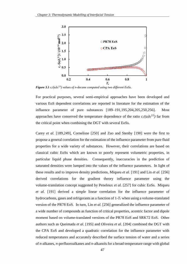
Chapter 3: Thermodynamic Modelling of Interfacial Tension
47
Figure 3.1 ci/(aibi
2/3) values of n-decane computed using two different EoSs.
For practical purposes, several semi-empirical approaches have been developed and
various EoS dependent correlations are reported in literature for the estimation of the
influence parameter of pure substances [189–191,195,204,205,250,256]. Most
approaches have conserved the temperature dependence of the ratio ci/(aibi2/3) far from
the critical point when combining the DGT with several EoSs.
Carey et al. [189,249], Cornelisse [250] and Zuo and Stenby [190] were the first to
propose a general correlation for the estimation of the influence parameter from pure fluid
properties for a wide variety of substances. However, their correlations are based on
classical cubic EoSs which are known to poorly represent volumetric properties, in
particular liquid phase densities. Consequently, inaccuracies in the prediction of
saturated densities were lumped into the values of the influence parameters. In light of
these results and to improve density predictions, Miqueu et al. [191] and Lin et al. [256]
derived correlations for the gradient theory influence parameter using the
volume-translation concept suggested by Peneloux et al. [257] for cubic EoSs. Miqueu
et al. [191] derived a simple linear correlation for the influence parameter of
hydrocarbons, gases and refrigerants as a function of 1-Tr when using a volume-translated
version of the PR78 EoS. In turn, Lin et al. [256] generalized the influence parameter of
a wide number of compounds as function of critical properties, acentric factor and dipole
moment based on volume-translated versions of the PR78 EoS and SRK72 EoS. Other
authors such as Queimada et al. [195] and Oliveira et al. [204] combined the DGT with
the CPA EoS and developed a quadratic correlation for the influence parameter with
reduced temperatures and accurately described the surface tension of water and a series
of n-alkanes, n-perfluoroalkanes and n-alkanols for a broad temperature range with global
Chapter 3: Thermodynamic Modelling of Interfacial Tension
48
average errors lower than 1 %. This work was also extended to several ester compounds
and their mixtures (biodiesels) by the same authors [205,206]. Another approach used by
several authors [61,204,216–218] consists of taking the influence parameter as a constant
value, usually calculated from surface tension data far from the critical point. Most
recently, the findings of Khosharay and co-workers [220,221,258] suggested that an
influence parameter dependent on both bulk liquid and vapour densities would produce
better results [258], in particular for aqueous systems [220,221].
Due to its simplicity and applicability to reservoir fluids [192,194,196], the expression
derived by Miqueu et al. [191] is adopted in this work for the estimation of the influence
parameter of systems containing non-polar and/or weakly polar substances such as
n-alkanes and common gases (CO2, CH4 and N2). This expression has the following form
[191]:
1610
1.2326 1.3757i
i
A
3.27
1610
0.9051 1.5410i
i
B
3.28
2/3
,1i i r i i i ic A T B a b 3.29
,
,
c i
r i
TT
T 3.30
where Tc,i and ωi correspond to the critical temperature and acentric factor of component
i, respectively, and ai and bi are the energy and co-volume parameters of the PR78 EoS.
This correlation was derived using properties in sub-critical conditions. Thus, the
influence parameter of pure fluids at or above supercritical conditions is estimated using
the generalized Equation 3.29 and by setting Tr to a fixed value. In this work, Tr is fixed
to the upper limit of temperatures considered by Miqueu et al. [191] and hence, the
influence parameters of supercritical CO2, CH4 and N2 are estimated for Tr = 0.96, 0.94
and 0.87, respectively. This procedure is adopted from Zuo and Stenby [190].
In contrast, the influence parameters of substances in aqueous systems are estimated using
two different approaches. The first consisted on taking the influence parameters to be
constant. These parameters are estimated using the empirical correlations regressed by
Queimada et al. [195] for water and Oliveira et al. [204] for n-alkanes and calculated for
Chapter 3: Thermodynamic Modelling of Interfacial Tension
49
a fixed value of Tr. The influence parameters of CO2, CH4 and N2 are regressed with
Equation 3.25 using surface tension data from REFPROP [99] at one temperature. The
influence parameters of some substances of interest estimated with this approach are
listed in Table 3.2 along with the percentage average absolute deviation (%AAD)2 to ST
data [99,259].
The second approach consisted on adopting the method suggested by Khosharay and co-
workers [220,221,258]. Accordingly, the influence parameters of pure substances
calculated from Equation 3.25 are expressed as function of bulk vapour and liquid molar
densities by [220,221,258]:
L V
i V L
i i
cA B
3.31
where Ai and Bi are the regression coefficients for component i.
For multicomponent systems, the influence parameters of component i with this approach
are calculated from the regressed coefficients (Ai and Bi) and the molar fraction of
component i in the coexisting bulk phases and are given by:
I II
i ii II I
i i i i
y xc
A x B y
3.32
The values of Ai and Bi for substances of interest are obtained by fitting Equation 3.31 to
the influence parameters calculated from Equation 3.25 using surface tension data. The
required ST data are taken from REFPROP [99] for water, gases, n-hexane and n-decane
and from the DIPPR database [259] for n-hexadecane. Two different sets of coefficients
are regressed:
The first set is fitted against surface tension data over a broad range of
reduced temperatures, as done in the works of Khosharay et al. [220,221,258];
For the second set, the influence parameters are considered to be
temperature independent and the coefficients fitted against surface tension data at the
lowest reduced temperatures. This temperature was selected as opposed to the highest to
2 mod% 1/ ( ) 100Exp ExpNP el
i i iiAAD NP X X X where X is the property under evaluation.
Chapter 3: Thermodynamic Modelling of Interfacial Tension
50
avoid most of the errors that arise from inappropriate prediction of saturated pure densities
by the CPA EoS near the critical point [195]; this behaviour is similar to that of classical
equation of states, such as cubics and generalised van der Waals’ equations, which do not
take into account fluctuations of the density of fluids near the vicinity of the critical point
[260].
The fitted coefficients Ai and Bi for some substances of interest are given in Tables 3.3
and 3.4 and, as an example, a comparison between the approaches for water, carbon
dioxide and n-decane is plotted in Figure 3.2.
As can be seen in Figure 3.2, all approaches provide a good description of the surface
tension of pure components. The lowest deviations were obtained with the method
proposed by Khosharay and co-workers and with the coefficients Ai and Bi fitted using
surface tension data over a broad range of reduced temperatures, as could be expected,
with an overall %AAD of 2.0 % (Table 3.3). On the other hand, the influence parameters
and coefficients Ai and Bi regressed at fixed Tr resulted in an increase of deviations to
experimental ST data, as listed in Table 3.2 and Table 3.4. This deterioration is partly
related to the wide range of temperatures considered, but also to the poor description of
the saturation properties by the phase equilibrium model near the critical region [195].
Nonetheless, using a constant influence parameter or as function of bulk densities fitted
at low temperatures allowed an estimation of the ST of pure fluids with an overall %AAD
of 5.7 and 4.3 %, respectively.
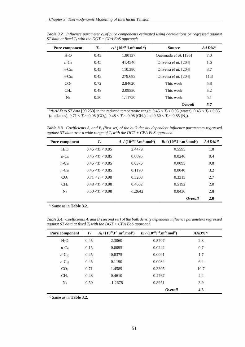
Chapter 3: Thermodynamic Modelling of Interfacial Tension
51
Table 3.2. Influence parameter ci of pure components estimated using correlations or regressed against
ST data at fixed Tr with the DGT + CPA EoS approach.
Pure component Tr ci / (10-20 J.m5.mol-2) Source AAD%a)
H2O 0.45 1.80137 Queimada et al. [195] 7.0
n-C6 0.45 41.4546 Oliveira et al. [204] 1.6
n-C10 0.45 110.380 Oliveira et al. [204] 3.7
n-C16 0.45 279.683 Oliveira et al. [204] 11.3
CO2 0.72 2.84620 This work 5.8
CH4 0.48 2.09550 This work 5.2
N2 0.50 1.11750 This work 5.1
Overall 5.7
a)%AAD to ST data [99,259] in the reduced temperature range: 0.45 < Tr < 0.95 (water), 0.45 < Tr < 0.85
(n-alkanes), 0.71 < Tr < 0.98 (CO2), 0.48 < Tr < 0.98 (CH4) and 0.50 < Tr < 0.85 (N2).
Table 3.3. Coefficients Ai and Bi (first set) of the bulk density dependent influence parameters regressed
against ST data over a wide range of Tr with the DGT + CPA EoS approach.
Pure component Tr Ai / (1020J-1.m-5.mol2) Bi / (1020J-1.m-5.mol2) AAD% a)
H2O 0.45 <Tr < 0.95 2.4479 0.5595 1.8
n-C6 0.45 <Tr < 0.85 0.0095 0.0246 0.4
n-C10 0.45 <Tr < 0.85 0.0375 0.0095 0.8
n-C16 0.45 <Tr < 0.85 0.1190 0.0040 3.2
CO2 0.71 <Tr< 0.98 0.3208 0.3315 2.7
CH4 0.48 <Tr < 0.98 0.4602 0.5192 2.0
N2 0.50 <Tr < 0.98 -1.2642 0.8436 2.8
Overall 2.0
a) Same as in Table 3.2.
Table 3.4. Coefficients Ai and Bi (second set) of the bulk density dependent influence parameters regressed
against ST data at fixed Tr with the DGT + CPA EoS approach.
Pure component Tr Ai / (1020J-1.m-5.mol2) Bi / (1020J-1.m-5.mol2) AAD% a)
H2O 0.45 2.3060 0.5707 2.3
n-C6 0.15 0.0095 0.0242 0.7
n-C10 0.45 0.0375 0.0091 1.7
n-C16 0.45 0.1190 0.0034 6.4
CO2 0.71 1.4589 0.3305 10.7
CH4 0.48 0.4610 0.4767 4.2
N2 0.50 -1.2678 0.8951 3.9
Overall 4.3
a) Same as in Table 3.2.
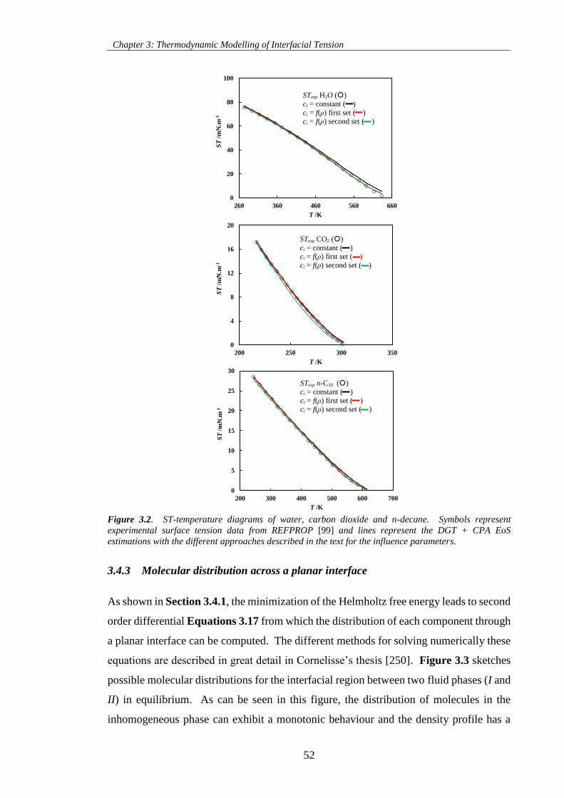
Chapter 3: Thermodynamic Modelling of Interfacial Tension
52
Figure 3.2. ST-temperature diagrams of water, carbon dioxide and n-decane. Symbols represent
experimental surface tension data from REFPROP [99] and lines represent the DGT + CPA EoS
estimations with the different approaches described in the text for the influence parameters.
3.4.3 Molecular distribution across a planar interface
As shown in Section 3.4.1, the minimization of the Helmholtz free energy leads to second
order differential Equations 3.17 from which the distribution of each component through
a planar interface can be computed. The different methods for solving numerically these
equations are described in great detail in Cornelisse’s thesis [250]. Figure 3.3 sketches
possible molecular distributions for the interfacial region between two fluid phases (I and
II) in equilibrium. As can be seen in this figure, the distribution of molecules in the
inhomogeneous phase can exhibit a monotonic behaviour and the density profile has a
0
20
40
60
80
100
260 360 460 560 660
ST
/mN
.m-1
T /K
water ST
Estimated: cii=constant
first set
second set
cii = constant
cii = f(ρ) first set
cii = f(ρ) second set
0
4
8
12
16
20
200 250 300 350
ST
/mN
.m-1
T /K
carbon dioxide ST
cii constant
first set
second set
cii = constant
cii = f(ρ) first set
cii = f(ρ) second set
0
5
10
15
20
25
30
200 300 400 500 600 700
ST
/mN
.m-1
T /K
n-decane ST
cii constant
first set
second set
cii = constant
cii = f(ρ) first set
cii = f(ρ) second set
STexp H2O ()
ci = constant ( )
ci = f(ρ) first set ( ) ci = f(ρ) second set ( )
STexp CO2 ()
ci = constant ( ) ci = f(ρ) first set ( )
ci = f(ρ) second set ( )
STexp n-C10 () ci = constant ( )
ci = f(ρ) first set ( ) ci = f(ρ) second set ( )
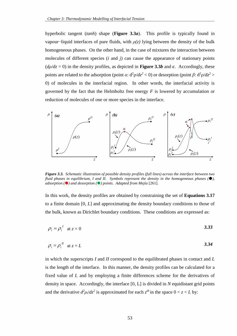
Chapter 3: Thermodynamic Modelling of Interfacial Tension
53
hyperbolic tangent (tanh) shape (Figure 3.3a). This profile is typically found in
vapour−liquid interfaces of pure fluids, with ρ(z) lying between the density of the bulk
homogeneous phases. On the other hand, in the case of mixtures the interaction between
molecules of different species (i and j) can cause the appearance of stationary points
(dρ/dz = 0) in the density profiles, as depicted in Figure 3.3b and c. Accordingly, these
points are related to the adsorption (point α: d2ρ/dz2 < 0) or desorption (point β: d2ρ/dz2 >
0) of molecules in the interfacial region. In other words, the interfacial activity is
governed by the fact that the Helmholtz free energy F is lowered by accumulation or
reduction of molecules of one or more species in the interface.
Figure 3.3. Schematic illustration of possible density profiles (full lines) across the interface between two
fluid phases in equilibrium, I and II. Symbols represent the density in the homogeneous phases (),
adsorption () and desorption () points. Adapted from Mejía [261].
In this work, the density profiles are obtained by constraining the set of Equations 3.17
to a finite domain [0, L] and approximating the density boundary conditions to those of
the bulk, known as Dirichlet boundary conditions. These conditions are expressed as:
I
i i at z = 0 3.33
II
i i at z = L 3.34
in which the superscripts I and II correspond to the equilibrated phases in contact and L
is the length of the interface. In this manner, the density profiles can be calculated for a
fixed value of L and by employing a finite differences scheme for the derivatives of
density in space. Accordingly, the interface [0, L] is divided in N equidistant grid points
and the derivative d2ρi/dz2 is approximated for each zth in the space 0 < z < L by:
Chapter 3: Thermodynamic Modelling of Interfacial Tension
54
2
1 1
2 2
12
th th thth z z zii i i
dz
dz z
3.35
The resultant set of non-linear equations is solved by a Newton-Raphson iteration scheme
together with the boundary conditions given in Equations 3.33 and 3.34. Since the
interface thickness is not known a priori, L is first estimated and subsequently enlarged
until the variation of the IFT values computed with Equation 3.23 is lower than 0.1 %.
This procedure ensures that only one solution exists. Usually initial values of L = 0.5 nm
sufficed for the method to converge at each enlargement of the interface. The
convergence criterion used for the density profiles at each intermediate value of L is
|ρi(zth)/dρi(z
th)| < 10-4. As suggested by Cornelisse [250], a linear distribution of each
component across the interfacial region is used as first guess of the density profiles for
the first estimate of L. The number of equations to solve at each enlargement of L is equal
to (N 2)×Ncomp and hence, N must be selected carefully to avoid not only numerical
problems, but also impracticable computation times. In this work, N = 500 proven to be
sufficient for the type of systems investigated.
The procedure described above allows the computation of the density profiles in a mixture
without any prior assumption on the distribution of the components across the interface
and is the method of choice if computation time is not a problem. However, taking cij to
be equal to the geometric mean (βij = 0) greatly simplifies Equations 3.17 and the
problem to be solved is reduced to a system of algebraic equations defined as
[192,194,248,250]:
0 . 0 .
1 1( ,..., ) ( ,..., )comp comp
Eq Eq
i ref N ref ref i N ic c
3.36
where i = 1…Ncomp 1 and the subscript ref denotes the reference component of the
mixture (i ≠ ref).
It is clear from the previous simplification that the density profile of each component can
be computed as roots of the algebraic Equations 3.36, i.e., the density of one component
(dependent variable, i) can be described as function of the density of the other one, in
which the latter is used as an independent (reference, ref) variable in a Newton-Raphson
root finding scheme. The selection of the reference component density needs to be done
with care, as it needs to be a monotonic function of z over the entire interfacial region
[192,248,250,262,263]. Since it is not known beforehand whether or not the density of a
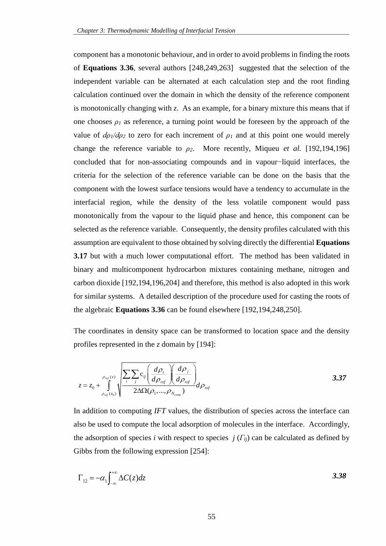
Chapter 3: Thermodynamic Modelling of Interfacial Tension
55
component has a monotonic behaviour, and in order to avoid problems in finding the roots
of Equations 3.36, several authors [248,249,263] suggested that the selection of the
independent variable can be alternated at each calculation step and the root finding
calculation continued over the domain in which the density of the reference component
is monotonically changing with z. As an example, for a binary mixture this means that if
one chooses ρ1 as reference, a turning point would be foreseen by the approach of the
value of dρ1/dρ2 to zero for each increment of ρ1 and at this point one would merely
change the reference variable to ρ2. More recently, Miqueu et al. [192,194,196]
concluded that for non-associating compounds and in vapour−liquid interfaces, the
criteria for the selection of the reference variable can be done on the basis that the
component with the lowest surface tensions would have a tendency to accumulate in the
interfacial region, while the density of the less volatile component would pass
monotonically from the vapour to the liquid phase and hence, this component can be
selected as the reference variable. Consequently, the density profiles calculated with this
assumption are equivalent to those obtained by solving directly the differential Equations
3.17 but with a much lower computational effort. The method has been validated in
binary and multicomponent hydrocarbon mixtures containing methane, nitrogen and
carbon dioxide [192,194,196,204] and therefore, this method is also adopted in this work
for similar systems. A detailed description of the procedure used for casting the roots of
the algebraic Equations 3.36 can be found elsewhere [192,194,248,250].
The coordinates in density space can be transformed to location space and the density
profiles represented in the z domain by [194]:
0
( )
0
1( )
c
2 ( ,..., )
ref
compref
jiijz
i j ref ref
ref
Nz
dd
d dz z d
3.37
In addition to computing IFT values, the distribution of species across the interface can
also be used to compute the local adsorption of molecules in the interface. Accordingly,
the adsorption of species i with respect to species j (Γij) can be calculated as defined by
Gibbs from the following expression [254]:
12 1 ( )C z dz
3.38
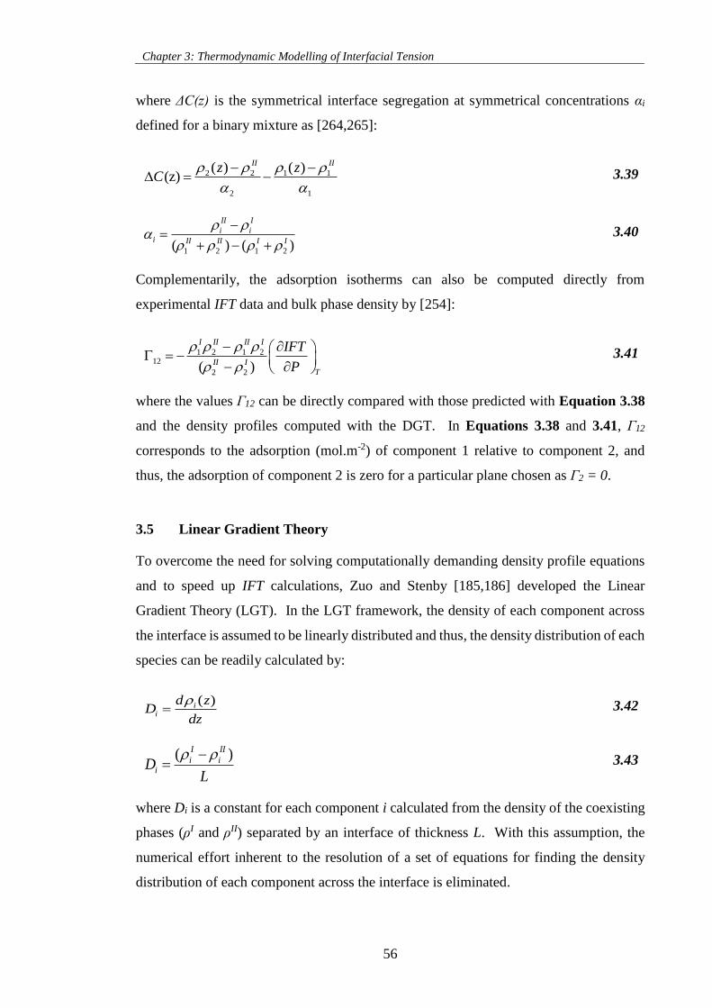
Chapter 3: Thermodynamic Modelling of Interfacial Tension
56
where ΔC(z) is the symmetrical interface segregation at symmetrical concentrations αi
defined for a binary mixture as [264,265]:
2 2 1 1
2 1
( ) ( )(z)
II IIz zC
3.39
1 2 1 2( ) ( )
II I
i ii II II I I
3.40
Complementarily, the adsorption isotherms can also be computed directly from
experimental IFT data and bulk phase density by [254]:
1 2 1 212
2 2( )
I II II I
II I
T
IFT
P
3.41
where the values Γ12 can be directly compared with those predicted with Equation 3.38
and the density profiles computed with the DGT. In Equations 3.38 and 3.41, Γ12
corresponds to the adsorption (mol.m-2) of component 1 relative to component 2, and
thus, the adsorption of component 2 is zero for a particular plane chosen as Γ2 = 0.
3.5 Linear Gradient Theory
To overcome the need for solving computationally demanding density profile equations
and to speed up IFT calculations, Zuo and Stenby [185,186] developed the Linear
Gradient Theory (LGT). In the LGT framework, the density of each component across
the interface is assumed to be linearly distributed and thus, the density distribution of each
species can be readily calculated by:
( )ii
d zD
dz
3.42
( )I II
i iiD
L
3.43
where Di is a constant for each component i calculated from the density of the coexisting
phases (ρI and ρII) separated by an interface of thickness L. With this assumption, the
numerical effort inherent to the resolution of a set of equations for finding the density
distribution of each component across the interface is eliminated.
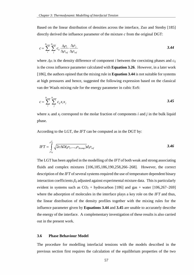
Chapter 3: Thermodynamic Modelling of Interfacial Tension
57
Based on the linear distribution of densities across the interface, Zuo and Stenby [185]
directly derived the influence parameter of the mixture c from the original DGT:
comp compN N
jiij
i j ref ref
c c
3.44
where Δρi is the density difference of component i between the coexisting phases and cij
is the cross influence parameter calculated with Equation 3.26. However, in a later work
[186], the authors opined that the mixing rule in Equation 3.44 is not suitable for systems
at high pressures and hence, suggested the following expression based on the classical
van der Waals mixing rule for the energy parameter in cubic EoS:
comp compN N
ij i j
i j
c c x x 3.45
where xi and xj correspond to the molar fraction of components i and j in the bulk liquid
phase.
According to the LGT, the IFT can be computed as in the DGT by:
12 ( ,..., )
IIref
Iref
Ncomp refIFT c d
3.46
The LGT has been applied in the modelling of the IFT of both weak and strong associating
fluids and complex mixtures [106,185,186,190,258,266–268]. However, the correct
description of the IFT of several systems required the use of temperature dependent binary
interaction coefficients βij adjusted against experimental mixture data. This is particularly
evident in systems such as CO2 + hydrocarbon [186] and gas + water [106,267–269]
where the adsorption of molecules in the interface plays a key role on the IFT and thus,
the linear distribution of the density profiles together with the mixing rules for the
influence parameter given by Equations 3.44 and 3.45 are unable to accurately describe
the energy of the interface. A complementary investigation of these results is also carried
out in the present work.
3.6 Phase Behaviour Model
The procedure for modelling interfacial tensions with the models described in the
previous section first requires the calculation of the equilibrium properties of the two
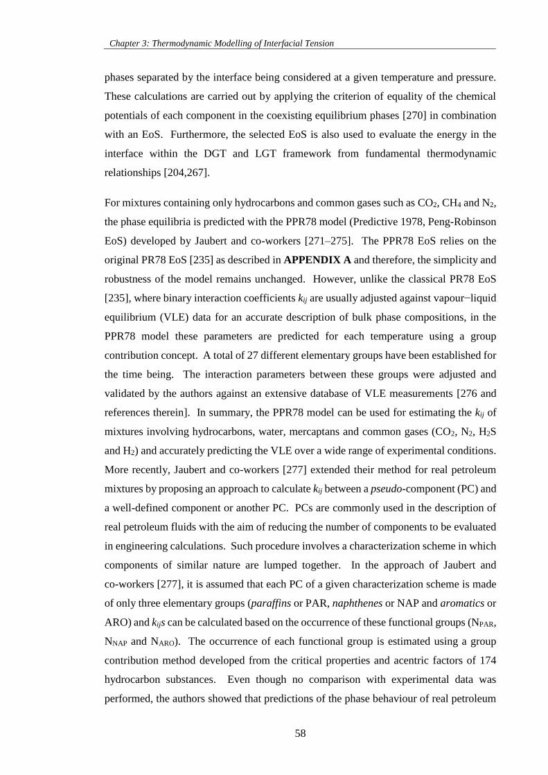
Chapter 3: Thermodynamic Modelling of Interfacial Tension
58
phases separated by the interface being considered at a given temperature and pressure.
These calculations are carried out by applying the criterion of equality of the chemical
potentials of each component in the coexisting equilibrium phases [270] in combination
with an EoS. Furthermore, the selected EoS is also used to evaluate the energy in the
interface within the DGT and LGT framework from fundamental thermodynamic
relationships [204,267].
For mixtures containing only hydrocarbons and common gases such as CO2, CH4 and N2,
the phase equilibria is predicted with the PPR78 model (Predictive 1978, Peng-Robinson
EoS) developed by Jaubert and co-workers [271–275]. The PPR78 EoS relies on the
original PR78 EoS [235] as described in APPENDIX A and therefore, the simplicity and
robustness of the model remains unchanged. However, unlike the classical PR78 EoS
[235], where binary interaction coefficients kij are usually adjusted against vapour−liquid
equilibrium (VLE) data for an accurate description of bulk phase compositions, in the
PPR78 model these parameters are predicted for each temperature using a group
contribution concept. A total of 27 different elementary groups have been established for
the time being. The interaction parameters between these groups were adjusted and
validated by the authors against an extensive database of VLE measurements [276 and
references therein]. In summary, the PPR78 model can be used for estimating the kij of
mixtures involving hydrocarbons, water, mercaptans and common gases (CO2, N2, H2S
and H2) and accurately predicting the VLE over a wide range of experimental conditions.
More recently, Jaubert and co-workers [277] extended their method for real petroleum
mixtures by proposing an approach to calculate kij between a pseudo-component (PC) and
a well-defined component or another PC. PCs are commonly used in the description of
real petroleum fluids with the aim of reducing the number of components to be evaluated
in engineering calculations. Such procedure involves a characterization scheme in which
components of similar nature are lumped together. In the approach of Jaubert and
co-workers [277], it is assumed that each PC of a given characterization scheme is made
of only three elementary groups (paraffins or PAR, naphthenes or NAP and aromatics or
ARO) and kijs can be calculated based on the occurrence of these functional groups (NPAR,
NNAP and NARO). The occurrence of each functional group is estimated using a group
contribution method developed from the critical properties and acentric factors of 174
hydrocarbon substances. Even though no comparison with experimental data was
performed, the authors showed that predictions of the phase behaviour of real petroleum
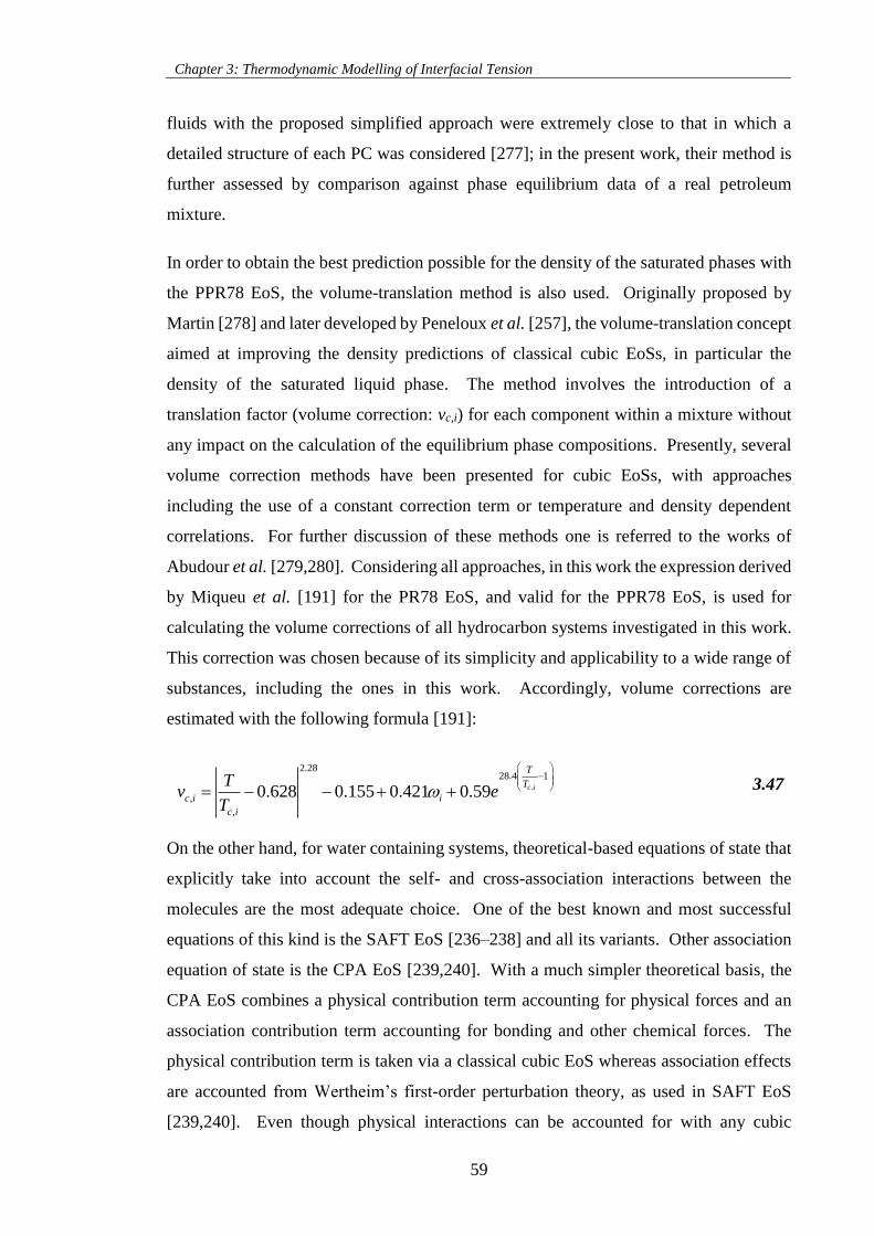
Chapter 3: Thermodynamic Modelling of Interfacial Tension
59
fluids with the proposed simplified approach were extremely close to that in which a
detailed structure of each PC was considered [277]; in the present work, their method is
further assessed by comparison against phase equilibrium data of a real petroleum
mixture.
In order to obtain the best prediction possible for the density of the saturated phases with
the PPR78 EoS, the volume-translation method is also used. Originally proposed by
Martin [278] and later developed by Peneloux et al. [257], the volume-translation concept
aimed at improving the density predictions of classical cubic EoSs, in particular the
density of the saturated liquid phase. The method involves the introduction of a
translation factor (volume correction: vc,i) for each component within a mixture without
any impact on the calculation of the equilibrium phase compositions. Presently, several
volume correction methods have been presented for cubic EoSs, with approaches
including the use of a constant correction term or temperature and density dependent
correlations. For further discussion of these methods one is referred to the works of
Abudour et al. [279,280]. Considering all approaches, in this work the expression derived
by Miqueu et al. [191] for the PR78 EoS, and valid for the PPR78 EoS, is used for
calculating the volume corrections of all hydrocarbon systems investigated in this work.
This correction was chosen because of its simplicity and applicability to a wide range of
substances, including the ones in this work. Accordingly, volume corrections are
estimated with the following formula [191]:
,
2.2828.4 1
,
,
0.628 0.155 0.421 0.59 c i
T
T
c i i
c i
Tv e
T
3.47
On the other hand, for water containing systems, theoretical-based equations of state that
explicitly take into account the self- and cross-association interactions between the
molecules are the most adequate choice. One of the best known and most successful
equations of this kind is the SAFT EoS [236–238] and all its variants. Other association
equation of state is the CPA EoS [239,240]. With a much simpler theoretical basis, the
CPA EoS combines a physical contribution term accounting for physical forces and an
association contribution term accounting for bonding and other chemical forces. The
physical contribution term is taken via a classical cubic EoS whereas association effects
are accounted from Wertheim’s first-order perturbation theory, as used in SAFT EoS
[239,240]. Even though physical interactions can be accounted for with any cubic
Chapter 3: Thermodynamic Modelling of Interfacial Tension
60
equation of state, the SRK72 EoS [234] is most commonly used and hence, it is also
adopted in this work, as described briefly in APPENDIX B. According to the CPA EoS
framework, non-associating molecules are defined by three molecular parameters (a0, c1
and b) and for associating molecules, two more parameters are included to model the
associating interactions (ε: association energy and βCPA: association volume). CPA
parameters are typically regressed simultaneously against experimental vapour pressure
and saturated liquid density data of pure compounds and thus, a good representation of
the volumetric properties of mixtures is usually obtained.
The CPA EoS has been shown to be able to properly describe the phase equilibria of water
with alkanes, cycloalkanes and alkenes [281,282], aromatics [282,283], alcohols [284],
glycols [285,286], fluoralkanes [287] and common gases such as CO2 [288], CH4 [289]
and N2 [290].
With relevance for this work, Tsivintzelis et al. [288] and Oliveira et al. [291,292]
investigated the CPA EoS description of the phase equilibria of CO2 binary mixtures with
water, alcohols, glycols, hydrocarbons, alcohols, esters and acids, over a broad range of
temperatures and pressures. Although CO2 can be regarded as a non-associating
compound, the findings of Tsivintzelis et al. [288] revealed the importance of taking into
consideration the specific strong interactions between CO2 and water, mainly Lewis
electron donor-acceptor type. Accordingly, the best description is obtained when the
interactions are accounted for through the procedure proposed by Folas et al. [283], where
the solvation is taken into account via the modified combining rule CR-1 (APPENDIX
B), where the cross-association energy is taken as half of the water self-associating
association energy and the cross-association volume is regressed from equilibria
experimental data along with the binary interaction coefficient, kij. In this work, the
solvation is taken by considering one cross-associating site in the CO2 molecules and
using the binary coefficients regressed against solubility data over the temperature range
298 to 477 K reported in the work of Tsivintzelis et al. [288]. Water is modelled as a
self-associating fluid with a 4C association scheme (according to the terminology
introduced by Huang and Radosz [238]), in which the hydrogen bonding between the
hydrogen atoms and the lone pairs of the oxygen are considered. No other type of
cross-association or self-associating molecules are considered throughout this work.
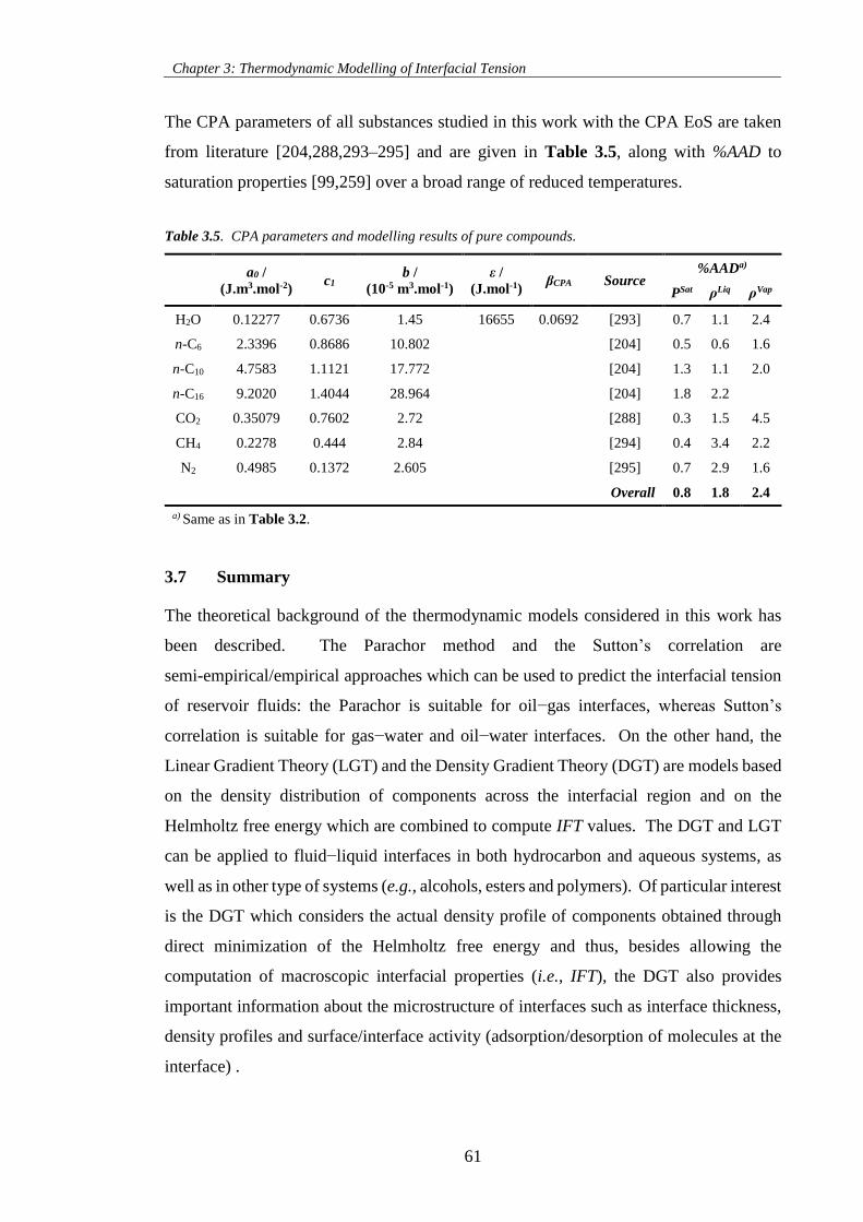
Chapter 3: Thermodynamic Modelling of Interfacial Tension
61
The CPA parameters of all substances studied in this work with the CPA EoS are taken
from literature [204,288,293–295] and are given in Table 3.5, along with %AAD to
saturation properties [99,259] over a broad range of reduced temperatures.
Table 3.5. CPA parameters and modelling results of pure compounds.
a0 /
(J.m3.mol-2) c1
b /
(10-5 m3.mol-1)
ε /
(J.mol-1) βCPA Source
%AADa)
PSat ρLiq ρVap
H2O 0.12277 0.6736 1.45 16655 0.0692 [293] 0.7 1.1 2.4
n-C6 2.3396 0.8686 10.802 [204] 0.5 0.6 1.6
n-C10 4.7583 1.1121 17.772 [204] 1.3 1.1 2.0
n-C16 9.2020 1.4044 28.964 [204] 1.8 2.2
CO2 0.35079 0.7602 2.72 [288] 0.3 1.5 4.5
CH4 0.2278 0.444 2.84 [294] 0.4 3.4 2.2
N2 0.4985 0.1372 2.605 [295] 0.7 2.9 1.6
Overall 0.8 1.8 2.4
a) Same as in Table 3.2.
3.7 Summary
The theoretical background of the thermodynamic models considered in this work has
been described. The Parachor method and the Sutton’s correlation are
semi-empirical/empirical approaches which can be used to predict the interfacial tension
of reservoir fluids: the Parachor is suitable for oil−gas interfaces, whereas Sutton’s
correlation is suitable for gas−water and oil−water interfaces. On the other hand, the
Linear Gradient Theory (LGT) and the Density Gradient Theory (DGT) are models based
on the density distribution of components across the interfacial region and on the
Helmholtz free energy which are combined to compute IFT values. The DGT and LGT
can be applied to fluid−liquid interfaces in both hydrocarbon and aqueous systems, as
well as in other type of systems (e.g., alcohols, esters and polymers). Of particular interest
is the DGT which considers the actual density profile of components obtained through
direct minimization of the Helmholtz free energy and thus, besides allowing the
computation of macroscopic interfacial properties (i.e., IFT), the DGT also provides
important information about the microstructure of interfaces such as interface thickness,
density profiles and surface/interface activity (adsorption/desorption of molecules at the
interface) .

Chapter 3: Thermodynamic Modelling of Interfacial Tension
62
In order to accurately describe the required bulk phase properties, the VT-PPR78 EoS
and the CPA EoS have been considered. The first is based on the classical cubic
Peng-Robinson 1978 EoS with volume corrections and a predictive feature for the
estimation of kij between mixture components. This EoS is used in CHAPTER 4 to
model the phase equilibria of the hydrocarbon systems examined. The second EoS is
suitable for modelling mixtures containing both inert and/or associating molecules. The
CPA Eos is used in CHAPTER 5 to model the phase equilibria of the aqueous systems
investigated. Furthermore, both EoSs are also used to evaluate the Helmholtz free energy
density of the interface within the DGT and LGT approaches.
63
CHAPTER 4 – INTERFACIAL TENSION OF HYDROCARBON
SYSTEMS
4.1 Introduction
As presented in CHAPTER 1, the deployment of more efficient and economical
extraction methods and processing facilities of oil and gas requires the accurate
knowledge of the interfacial tension of gas + oil systems. Thus, in this chapter an
experimental and modelling investigation on the IFT and density of oil + gas systems was
conducted for binary and multicomponent mixtures composed of n-alkanes and common
gases such as carbon dioxide, methane and nitrogen.
Aiming at filling the experimental gap found in literature (Section 1.3.1), saturated
density and IFT measurements of binary systems gas + n-decane (gas = CO2, CH4 and
N2) were extended for different isotherms (up to 442 K) and pressures up to 69 MPa or
near the critical point of each mixture. Measurements were carried out with the
experimental setup based on the Capillary Rise technique (Section 2.2) and both the
equipment and methodology were validated through comparison with selected
experimental data available in literature. Densities of the saturated phases were measured
with a high pressure densitometer and the data correlated with a thermodynamic phase
behaviour model based on the PR78 EoS (APPENDIX A). Modelled density data were
combined with measured capillary constants to estimate pertinent IFT values.
Complementarily, measurements were also carried out for three multicomponent
synthetic mixtures at a representative reservoir temperature of 393 K. The studied
synthetic mixtures comprised systems of up to 9 components which can be used to mimic
the behaviour of real gas condensate and petroleum mixtures, particularly during CO2
injection processes.
The development of predictive models capable of accurately accounting the effect of
temperature and pressure on the phase behaviour and IFT is necessary for the design of
more efficient oil recovery processes. Therefore, the predictive capabilities of the
Parachor, LGT and DGT approaches in combination with the VT-PPR78 EoS were
assessed by comparison with data measured in this work and gathered from literature for
hydrocarbon systems. This means that in the case of the LGT and DGT models the binary
coefficient in the mixing rule of the influence parameters was fixed to zero (i.e., βij = 0).
In total, 16 gas + n-alkane binary and 3 multicomponent synthetic mixtures as well as 1
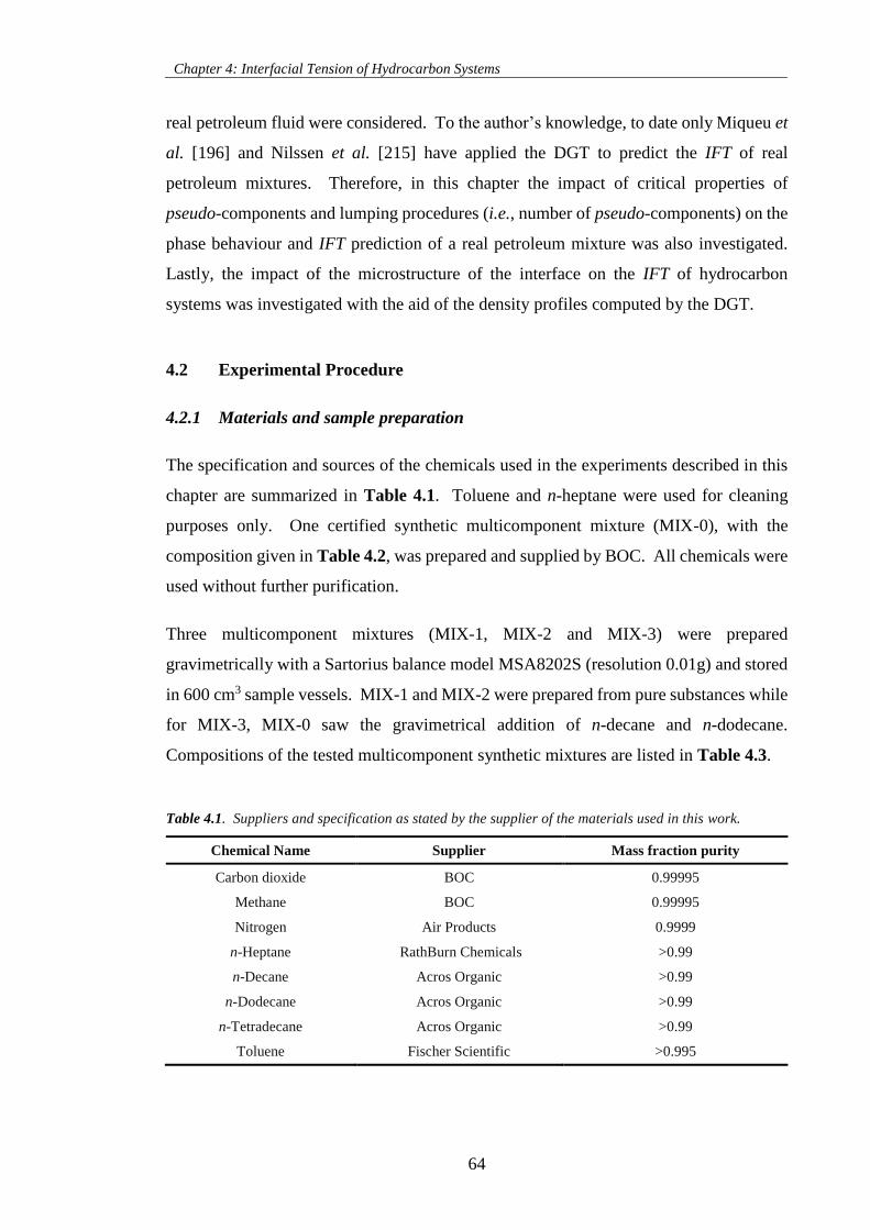
Chapter 4: Interfacial Tension of Hydrocarbon Systems
64
real petroleum fluid were considered. To the author’s knowledge, to date only Miqueu et
al. [196] and Nilssen et al. [215] have applied the DGT to predict the IFT of real
petroleum mixtures. Therefore, in this chapter the impact of critical properties of
pseudo-components and lumping procedures (i.e., number of pseudo-components) on the
phase behaviour and IFT prediction of a real petroleum mixture was also investigated.
Lastly, the impact of the microstructure of the interface on the IFT of hydrocarbon
systems was investigated with the aid of the density profiles computed by the DGT.
4.2 Experimental Procedure
4.2.1 Materials and sample preparation
The specification and sources of the chemicals used in the experiments described in this
chapter are summarized in Table 4.1. Toluene and n-heptane were used for cleaning
purposes only. One certified synthetic multicomponent mixture (MIX-0), with the
composition given in Table 4.2, was prepared and supplied by BOC. All chemicals were
used without further purification.
Three multicomponent mixtures (MIX-1, MIX-2 and MIX-3) were prepared
gravimetrically with a Sartorius balance model MSA8202S (resolution 0.01g) and stored
in 600 cm3 sample vessels. MIX-1 and MIX-2 were prepared from pure substances while
for MIX-3, MIX-0 saw the gravimetrical addition of n-decane and n-dodecane.
Compositions of the tested multicomponent synthetic mixtures are listed in Table 4.3.
Table 4.1. Suppliers and specification as stated by the supplier of the materials used in this work.
Chemical Name Supplier Mass fraction purity
Carbon dioxide BOC 0.99995
Methane BOC 0.99995
Nitrogen Air Products 0.9999
n-Heptane RathBurn Chemicals >0.99
n-Decane Acros Organic >0.99
n-Dodecane Acros Organic >0.99
n-Tetradecane Acros Organic >0.99
Toluene Fischer Scientific >0.995
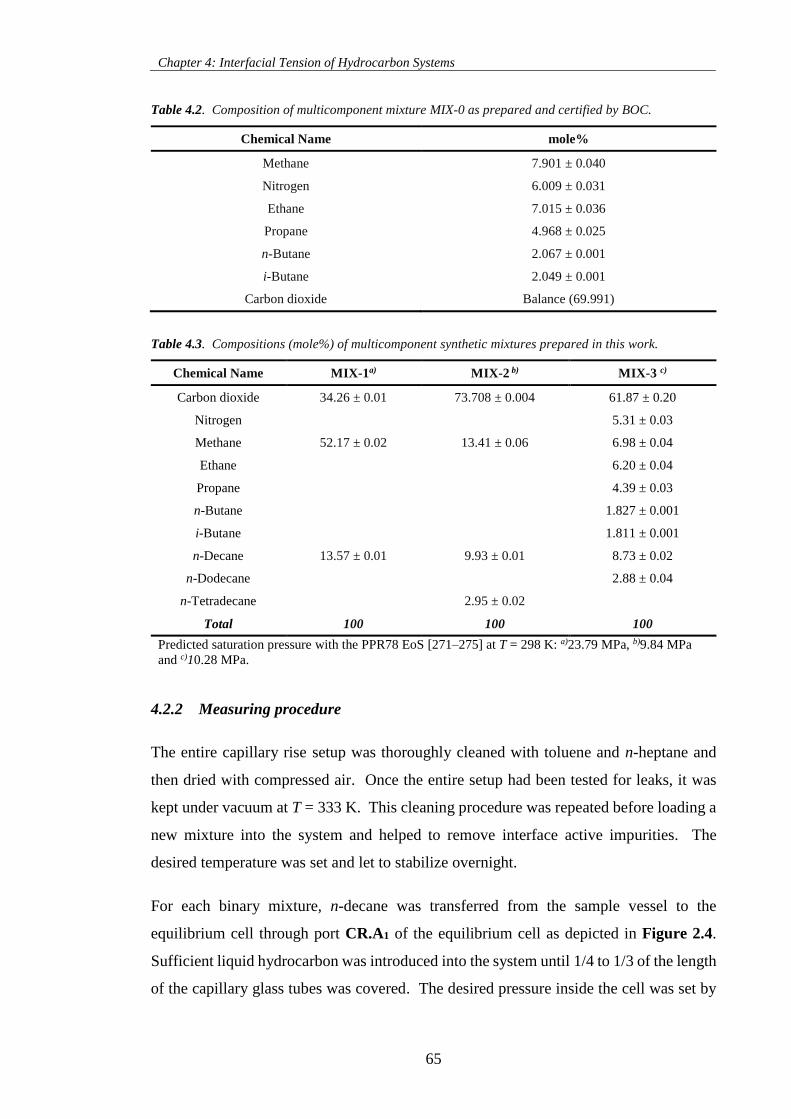
Chapter 4: Interfacial Tension of Hydrocarbon Systems
65
Table 4.2. Composition of multicomponent mixture MIX-0 as prepared and certified by BOC.
Chemical Name mole%
Methane 7.901 ± 0.040
Nitrogen 6.009 ± 0.031
Ethane 7.015 ± 0.036
Propane 4.968 ± 0.025
n-Butane 2.067 ± 0.001
i-Butane 2.049 ± 0.001
Carbon dioxide Balance (69.991)
Table 4.3. Compositions (mole%) of multicomponent synthetic mixtures prepared in this work.
Chemical Name MIX-1a) MIX-2 b) MIX-3 c)
Carbon dioxide 34.26 ± 0.01 73.708 ± 0.004 61.87 ± 0.20
Nitrogen 5.31 ± 0.03
Methane 52.17 ± 0.02 13.41 ± 0.06 6.98 ± 0.04
Ethane 6.20 ± 0.04
Propane 4.39 ± 0.03
n-Butane 1.827 ± 0.001
i-Butane 1.811 ± 0.001
n-Decane 13.57 ± 0.01 9.93 ± 0.01 8.73 ± 0.02
n-Dodecane 2.88 ± 0.04
n-Tetradecane 2.95 ± 0.02
Total 100 100 100
Predicted saturation pressure with the PPR78 EoS [271–275] at T = 298 K: a)23.79 MPa, b)9.84 MPa
and c)10.28 MPa.
4.2.2 Measuring procedure
The entire capillary rise setup was thoroughly cleaned with toluene and n-heptane and
then dried with compressed air. Once the entire setup had been tested for leaks, it was
kept under vacuum at T = 333 K. This cleaning procedure was repeated before loading a
new mixture into the system and helped to remove interface active impurities. The
desired temperature was set and let to stabilize overnight.
For each binary mixture, n-decane was transferred from the sample vessel to the
equilibrium cell through port CR.A1 of the equilibrium cell as depicted in Figure 2.4.
Sufficient liquid hydrocarbon was introduced into the system until 1/4 to 1/3 of the length
of the capillary glass tubes was covered. The desired pressure inside the cell was set by
Chapter 4: Interfacial Tension of Hydrocarbon Systems
66
injecting pure gas (i.e., methane, carbon dioxide or nitrogen) into the equilibrium cell and
controlling the back pressure of the sample vessel.
On the other hand, for multicomponent mixtures they were loaded into the equilibrium
cell by pumping hydraulic fluid behind the piston in the sample vessel containing the
testing fluid (MIX-1, MIX-2 or MIX-3) and the pressure inside the equilibrium cell
increased at successive steps by controlling the amount of sample transferred. The
pressure inside the sample vessel was maintained at values sufficiently higher than the
predicted saturation pressure at ambient temperature, i.e., T ≈ 298 K (Table 4.3), to ensure
that the tested mixture was in single-phase state at each loading step.
For each pressure and temperature state, valves CR1, CR4 and CR5 were kept closed and
the content of the cell was stirred until pressure and temperature readings were stabilized.
Once equilibrium was achieved, normally after 10 min, stirring was stopped and the liquid
rise in each capillary tube was measured.
The saturated liquid density was measured by displacing the phase in the equilibrium cell
into the densitometer whilst stirring. Opening valve CR5 and controlling the movement
of piston CR.D with the aid of the DBR pump, allowed the saturated liquid phase to be
displaced from the equilibrium cell into the densitometer, as depicted in Figure 2.4. The
injection and withdrawal of hydraulic fluid behind piston CR.D were performed at a
constant rate 100 cm3.h-1 with the control software of the pump. The back-flow of fluids
from the densitometer to the equilibrium cell was prevented by means of check valves
CR.E1 and CR.E2. Generally 4-5 cycles (~5 cm3/each) allowed a complete renewal of
the fluids inside the densitometer with a total pressure change in the system of not more
than 0.1 MPa at each stroke, ensuring that the equilibrium conditions were maintained.
Following this, the cycling was stopped, valve CR5 closed and the resonance period of
the vibrating tube (τ) recorded after a 5 min period of stabilization.
The measured period of vibration (τ) of a U-tube can be related to the density (ρ)
according to:
2
1 2D D
4.1
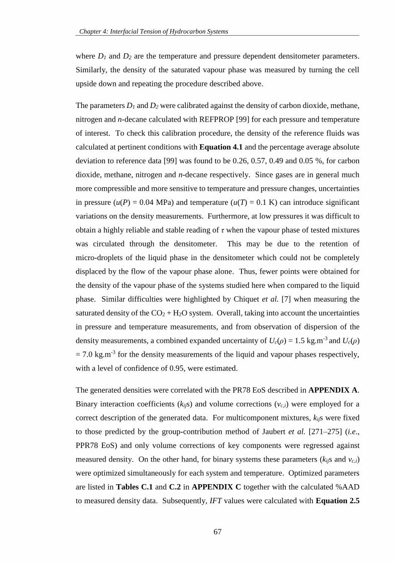
Chapter 4: Interfacial Tension of Hydrocarbon Systems
67
where D1 and D2 are the temperature and pressure dependent densitometer parameters.
Similarly, the density of the saturated vapour phase was measured by turning the cell
upside down and repeating the procedure described above.
The parameters D1 and D2 were calibrated against the density of carbon dioxide, methane,
nitrogen and n-decane calculated with REFPROP [99] for each pressure and temperature
of interest. To check this calibration procedure, the density of the reference fluids was
calculated at pertinent conditions with Equation 4.1 and the percentage average absolute
deviation to reference data [99] was found to be 0.26, 0.57, 0.49 and 0.05 %, for carbon
dioxide, methane, nitrogen and n-decane respectively. Since gases are in general much
more compressible and more sensitive to temperature and pressure changes, uncertainties
in pressure (u(P) = 0.04 MPa) and temperature (u(T) = 0.1 K) can introduce significant
variations on the density measurements. Furthermore, at low pressures it was difficult to
obtain a highly reliable and stable reading of τ when the vapour phase of tested mixtures
was circulated through the densitometer. This may be due to the retention of
micro-droplets of the liquid phase in the densitometer which could not be completely
displaced by the flow of the vapour phase alone. Thus, fewer points were obtained for
the density of the vapour phase of the systems studied here when compared to the liquid
phase. Similar difficulties were highlighted by Chiquet et al. [7] when measuring the
saturated density of the CO2 + H2O system. Overall, taking into account the uncertainties
in pressure and temperature measurements, and from observation of dispersion of the
density measurements, a combined expanded uncertainty of Uc(ρ) = 1.5 kg.m-3 and Uc(ρ)
= 7.0 kg.m-3 for the density measurements of the liquid and vapour phases respectively,
with a level of confidence of 0.95, were estimated.
The generated densities were correlated with the PR78 EoS described in APPENDIX A.
Binary interaction coefficients (kijs) and volume corrections (vc,i) were employed for a
correct description of the generated data. For multicomponent mixtures, kijs were fixed
to those predicted by the group-contribution method of Jaubert et al. [271–275] (i.e.,
PPR78 EoS) and only volume corrections of key components were regressed against
measured density. On the other hand, for binary systems these parameters (kijs and vc,i)
were optimized simultaneously for each system and temperature. Optimized parameters
are listed in Tables C.1 and C.2 in APPENDIX C together with the calculated %AAD
to measured density data. Subsequently, IFT values were calculated with Equation 2.5
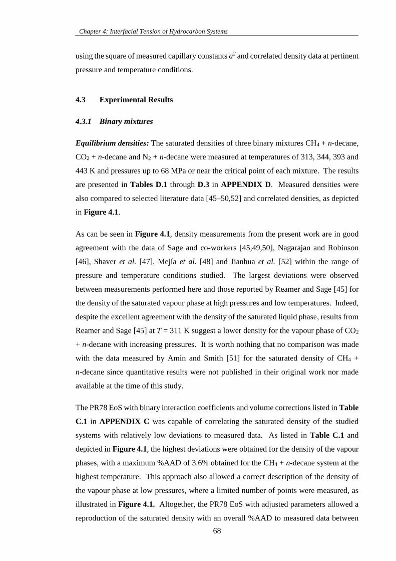
Chapter 4: Interfacial Tension of Hydrocarbon Systems
68
using the square of measured capillary constants a2 and correlated density data at pertinent
pressure and temperature conditions.
4.3 Experimental Results
4.3.1 Binary mixtures
Equilibrium densities: The saturated densities of three binary mixtures CH4 + n-decane,
CO2 + n-decane and N2 + n-decane were measured at temperatures of 313, 344, 393 and
443 K and pressures up to 68 MPa or near the critical point of each mixture. The results
are presented in Tables D.1 through D.3 in APPENDIX D. Measured densities were
also compared to selected literature data [45–50,52] and correlated densities, as depicted
in Figure 4.1.
As can be seen in Figure 4.1, density measurements from the present work are in good
agreement with the data of Sage and co-workers [45,49,50], Nagarajan and Robinson
[46], Shaver et al. [47], Mejía et al. [48] and Jianhua et al. [52] within the range of
pressure and temperature conditions studied. The largest deviations were observed
between measurements performed here and those reported by Reamer and Sage [45] for
the density of the saturated vapour phase at high pressures and low temperatures. Indeed,
despite the excellent agreement with the density of the saturated liquid phase, results from
Reamer and Sage [45] at T = 311 K suggest a lower density for the vapour phase of CO2
+ n-decane with increasing pressures. It is worth nothing that no comparison was made
with the data measured by Amin and Smith [51] for the saturated density of CH4 +
n-decane since quantitative results were not published in their original work nor made
available at the time of this study.
The PR78 EoS with binary interaction coefficients and volume corrections listed in Table
C.1 in APPENDIX C was capable of correlating the saturated density of the studied
systems with relatively low deviations to measured data. As listed in Table C.1 and
depicted in Figure 4.1, the highest deviations were obtained for the density of the vapour
phases, with a maximum %AAD of 3.6% obtained for the CH4 + n-decane system at the
highest temperature. This approach also allowed a correct description of the density of
the vapour phase at low pressures, where a limited number of points were measured, as
illustrated in Figure 4.1. Altogether, the PR78 EoS with adjusted parameters allowed a
reproduction of the saturated density with an overall %AAD to measured data between
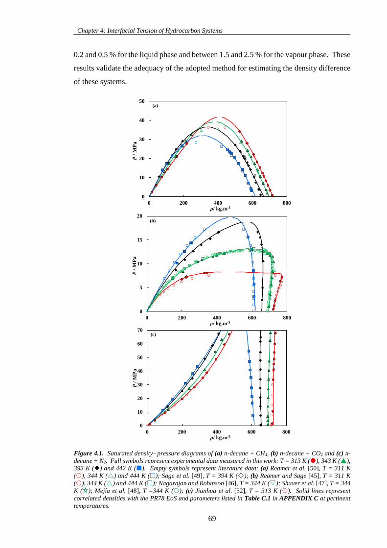
Chapter 4: Interfacial Tension of Hydrocarbon Systems
69
0.2 and 0.5 % for the liquid phase and between 1.5 and 2.5 % for the vapour phase. These
results validate the adequacy of the adopted method for estimating the density difference
of these systems.
Figure 4.1. Saturated density−pressure diagrams of (a) n-decane + CH4, (b) n-decane + CO2 and (c) n-
decane + N2. Full symbols represent experimental data measured in this work: T = 313 K (), 343 K (),
393 K () and 442 K (). Empty symbols represent literature data: (a) Reamer et al. [50], T = 311 K
(), 344 K () and 444 K (); Sage et al. [49], T = 394 K (); (b) Reamer and Sage [45], T = 311 K
(), 344 K () and 444 K (); Nagarajan and Robinson [46], T = 344 K (); Shaver et al. [47], T = 344
K ( ); Mejía et al. [48], T =344 K (); (c) Jianhua et al. [52], T = 313 K (). Solid lines represent
correlated densities with the PR78 EoS and parameters listed in Table C.1 in APPENDIX C at pertinent
temperatures.
0
10
20
30
40
50
0 200 400 600 800
P/
MP
a
ρ/ kg.m-3
0
5
10
15
20
0 200 400 600 800
P/
MP
a
ρ/ kg.m-3
0
10
20
30
40
50
60
70
0 200 400 600 800
P/
MP
a
ρ/ kg.m-3
(c)
(b)
(a)
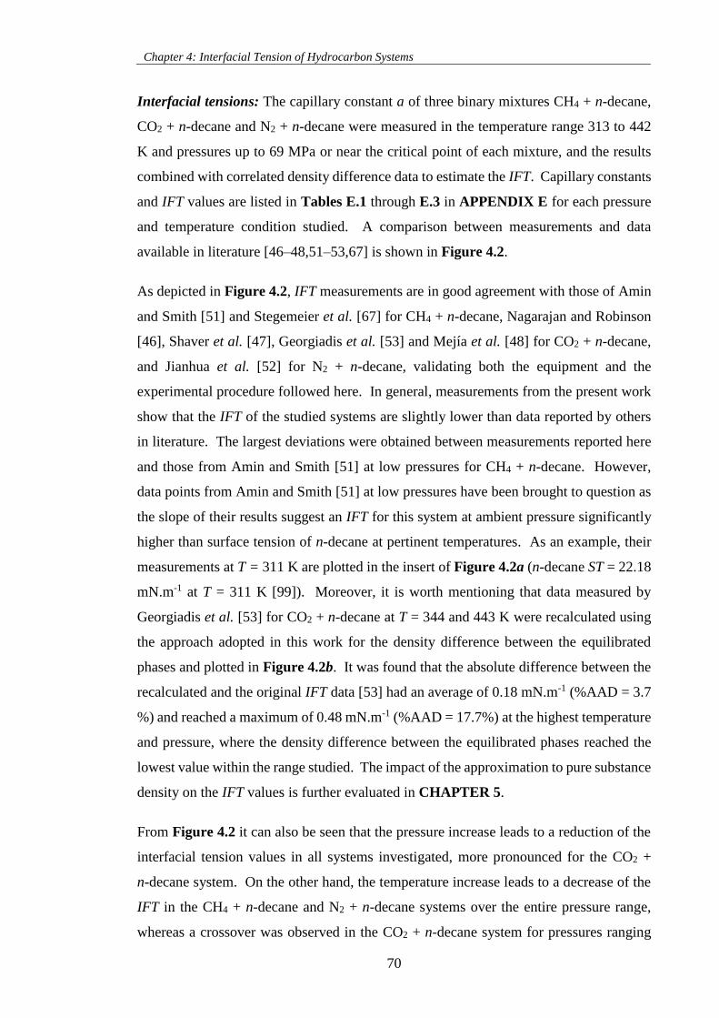
Chapter 4: Interfacial Tension of Hydrocarbon Systems
70
Interfacial tensions: The capillary constant a of three binary mixtures CH4 + n-decane,
CO2 + n-decane and N2 + n-decane were measured in the temperature range 313 to 442
K and pressures up to 69 MPa or near the critical point of each mixture, and the results
combined with correlated density difference data to estimate the IFT. Capillary constants
and IFT values are listed in Tables E.1 through E.3 in APPENDIX E for each pressure
and temperature condition studied. A comparison between measurements and data
available in literature [46–48,51–53,67] is shown in Figure 4.2.
As depicted in Figure 4.2, IFT measurements are in good agreement with those of Amin
and Smith [51] and Stegemeier et al. [67] for CH4 + n-decane, Nagarajan and Robinson
[46], Shaver et al. [47], Georgiadis et al. [53] and Mejía et al. [48] for CO2 + n-decane,
and Jianhua et al. [52] for N2 + n-decane, validating both the equipment and the
experimental procedure followed here. In general, measurements from the present work
show that the IFT of the studied systems are slightly lower than data reported by others
in literature. The largest deviations were obtained between measurements reported here
and those from Amin and Smith [51] at low pressures for CH4 + n-decane. However,
data points from Amin and Smith [51] at low pressures have been brought to question as
the slope of their results suggest an IFT for this system at ambient pressure significantly
higher than surface tension of n-decane at pertinent temperatures. As an example, their
measurements at T = 311 K are plotted in the insert of Figure 4.2a (n-decane ST = 22.18
mN.m-1 at T = 311 K [99]). Moreover, it is worth mentioning that data measured by
Georgiadis et al. [53] for CO2 + n-decane at T = 344 and 443 K were recalculated using
the approach adopted in this work for the density difference between the equilibrated
phases and plotted in Figure 4.2b. It was found that the absolute difference between the
recalculated and the original IFT data [53] had an average of 0.18 mN.m-1 (%AAD = 3.7
%) and reached a maximum of 0.48 mN.m-1 (%AAD = 17.7%) at the highest temperature
and pressure, where the density difference between the equilibrated phases reached the
lowest value within the range studied. The impact of the approximation to pure substance
density on the IFT values is further evaluated in CHAPTER 5.
From Figure 4.2 it can also be seen that the pressure increase leads to a reduction of the
interfacial tension values in all systems investigated, more pronounced for the CO2 +
n-decane system. On the other hand, the temperature increase leads to a decrease of the
IFT in the CH4 + n-decane and N2 + n-decane systems over the entire pressure range,
whereas a crossover was observed in the CO2 + n-decane system for pressures ranging
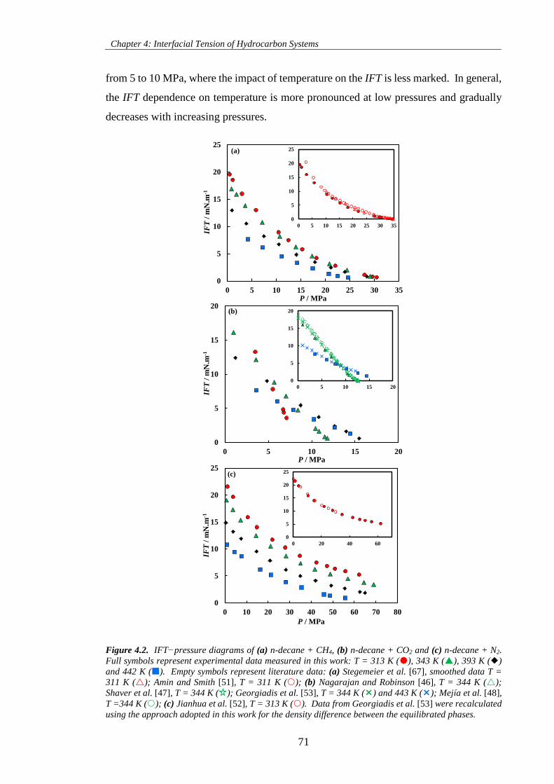
Chapter 4: Interfacial Tension of Hydrocarbon Systems
71
from 5 to 10 MPa, where the impact of temperature on the IFT is less marked. In general,
the IFT dependence on temperature is more pronounced at low pressures and gradually
decreases with increasing pressures.
Figure 4.2. IFT−pressure diagrams of (a) n-decane + CH4, (b) n-decane + CO2 and (c) n-decane + N2.
Full symbols represent experimental data measured in this work: T = 313 K (), 343 K (), 393 K ()
and 442 K (). Empty symbols represent literature data: (a) Stegemeier et al. [67], smoothed data T =
311 K (); Amin and Smith [51], T = 311 K (); (b) Nagarajan and Robinson [46], T = 344 K ();
Shaver et al. [47], T = 344 K ( ); Georgiadis et al. [53], T = 344 K () and 443 K (); Mejía et al. [48],
T =344 K (); (c) Jianhua et al. [52], T = 313 K (). Data from Georgiadis et al. [53] were recalculated
using the approach adopted in this work for the density difference between the equilibrated phases.
0
5
10
15
20
25
0 10 20 30 40 50 60 70 80
IFT
/ m
N.m
-1
P / MPa
0
5
10
15
20
25
0 20 40 60
0
5
10
15
20
25
0 5 10 15 20 25 30 35
IFT
/ m
N.m
-1
P / MPa
0
5
10
15
20
25
0 5 10 15 20 25 30 35
0
5
10
15
20
0 5 10 15 20
IFT
/ m
N.m
-1
P / MPa
0
5
10
15
20
0 5 10 15 20
(a)
(b)
(c)
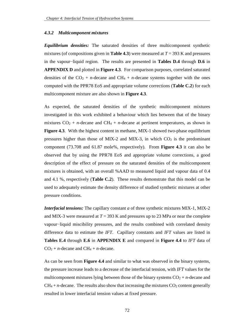
Chapter 4: Interfacial Tension of Hydrocarbon Systems
72
4.3.2 Multicomponent mixtures
Equilibrium densities: The saturated densities of three multicomponent synthetic
mixtures (of compositions given in Table 4.3) were measured at T = 393 K and pressures
in the vapour−liquid region. The results are presented in Tables D.4 through D.6 in
APPENDIX D and plotted in Figure 4.3. For comparison purposes, correlated saturated
densities of the CO2 + n-decane and CH4 + n-decane systems together with the ones
computed with the PPR78 EoS and appropriate volume corrections (Table C.2) for each
multicomponent mixture are also shown in Figure 4.3.
As expected, the saturated densities of the synthetic multicomponent mixtures
investigated in this work exhibited a behaviour which lies between that of the binary
mixtures CO2 + n-decane and CH4 + n-decane at pertinent temperatures, as shown in
Figure 4.3. With the highest content in methane, MIX-1 showed two-phase equilibrium
pressures higher than those of MIX-2 and MIX-3, in which CO2 is the predominant
component (73.708 and 61.87 mole%, respectively). From Figure 4.3 it can also be
observed that by using the PPR78 EoS and appropriate volume corrections, a good
description of the effect of pressure on the saturated densities of the multicomponent
mixtures is obtained, with an overall %AAD to measured liquid and vapour data of 0.4
and 4.1 %, respectively (Table C.2). These results demonstrate that this model can be
used to adequately estimate the density difference of studied synthetic mixtures at other
pressure conditions.
Interfacial tensions: The capillary constant a of three synthetic mixtures MIX-1, MIX-2
and MIX-3 were measured at T = 393 K and pressures up to 23 MPa or near the complete
vapour−liquid miscibility pressures, and the results combined with correlated density
difference data to estimate the IFT. Capillary constants and IFT values are listed in
Tables E.4 through E.6 in APPENDIX E and compared in Figure 4.4 to IFT data of
CO2 + n-decane and CH4 + n-decane.
As can be seen from Figure 4.4 and similar to what was observed in the binary systems,
the pressure increase leads to a decrease of the interfacial tension, with IFT values for the
multicomponent mixtures lying between those of the binary systems CO2 + n-decane and
CH4 + n-decane. The results also show that increasing the mixtures CO2 content generally
resulted in lower interfacial tension values at fixed pressure.
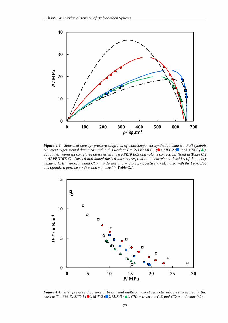
Chapter 4: Interfacial Tension of Hydrocarbon Systems
73
Figure 4.3. Saturated density−pressure diagrams of multicomponent synthetic mixtures. Full symbols
represent experimental data measured in this work at T = 393 K: MIX-1 (), MIX-2 () and MIX-3 ().
Solid lines represent correlated densities with the PPR78 EoS and volume corrections listed in Table C.2
in APPENDIX C. Dashed and dotted-dashed lines correspond to the correlated densities of the binary
mixtures CH4 + n-decane and CO2 + n-decane at T = 393 K, respectively, calculated with the PR78 EoS
and optimized parameters (kijs and vc,i) listed in Table C.1.
Figure 4.4. IFT−pressure diagrams of binary and multicomponent synthetic mixtures measured in this
work at T = 393 K: MIX-1 (), MIX-2 (), MIX-3 (), CH4 + n-decane () and CO2 + n-decane ().
0
10
20
30
40
0 100 200 300 400 500 600 700
P/
MP
a
ρ/ kg.m-3
0
5
10
15
0 5 10 15 20 25 30
IFT
/ m
N.m
-1
P/ MPa
Chapter 4: Interfacial Tension of Hydrocarbon Systems
74
4.3.3 Experimental uncertainties
The measurement of any thermophysical property is always susceptible to uncertainties
which affect the overall accuracy of experimental data. In this work, the combined
expanded uncertainties in the interfacial tension measurements, Uc (IFT), with the
differential CR method are assessed by considering the effect of uncertainties on the
measured capillary constants, U1 (IFT), and uncertainties on the estimation of the density
of the equilibrated phases, U2 (IFT).
U1 (IFT) can be estimated by considering the impact of uncertainties of the cathetometer
and dispersion of the measured difference of the liquid rise height in the capillary tubes,
Δh. It was estimated a combined expanded uncertainty for Δh of 0.010 cm for
measurements ranging from 1.876 to 0.129 cm, with a level of confidence of 0.95. The
calculation of the expanded uncertainty of a2 depends not only of the ID of the capillary
tubes, but also of the magnitude of Δh and, in turn, of the total pressure of the system.
For measurements performed with the CR setup, the combined expanded uncertainty of
a2 was found to be Uc (a2) = 0.000331 cm2, with a level of confidence of 0.95, yielding
expanded relative uncertainties for this parameter between 0.5 and 0.7 % at low pressures
and up to 8 % for pressures close to the complete vapour−liquid miscibility, where Δh
reached the lowest values. Using the law of propagation of errors [296], U1 (IFT) can be
estimated as follows:
1/22
2 2
1 2( ) ( )c
IFTU IFT U a
a
4.2
1/22
22 2( ) ( )c c
aU a U h
h
4.3
The second contribution, U2 (IFT), can be estimated by considering the deviations
between correlated and measured density data for each system, phase and temperature of
interest (Tables C.1 and C.2 in APPENDIX C). The impact of uncertainties in
temperature (u(T) = 0.1 K) and pressure (u(P) = 0.04 MPa), as well as mixtures
composition on the estimation of the density of the saturated phases, are somewhat
suppressed by the deviations of the model to measured data and hence, were not
considered. The expression for estimating U2 (IFT) has the following form [296]:
Chapter 4: Interfacial Tension of Hydrocarbon Systems
75
1/22 2
2 2
2 ( ) ( ) ( )L V
c cL V
IFT IFTU IFT U U
4.4
The combined expanded uncertainties in the IFT measurements estimated with a
confidence level of 0.95, are shown in Tables E.1 through E.6 for each system and
experimental condition, with values averaging 0.13, 0.12 and 0.14 mN.m-1 for CO2 +
n-decane, CH4 + n-decane and N2 + n-decane, respectively, and 0.10, 0.14 and 0.12
mN.m-1 for MIX-1, MIX-2 and MIX-3, respectively. Overall, the combined expanded
uncertainty of the IFT measurements increased with pressure, with relative expanded
uncertainties lower than 1.5% at low pressures and up to 11.3 % near the complete
miscibility conditions, where IFT values are very low (< 1.5 mN.m-1).
4.4 Modelling
4.4.1 Binary and multicomponent synthetic mixtures
In this section the predictive capabilities of the VT-PPR78 EoS and IFT models to
represent the experimental data of the studied synthetic hydrocarbon systems were
evaluated. This analysis was also extended to binary mixtures containing CH4, CO2 and
N2 and other n-alkanes by comparing the IFT predictions against selected literature data
[41,52,54,59,61,63,64,68,69,74].
Classical cubic equations of state have been extensively applied in previous studies
available in literature in combination with IFT methods to model the interfacial tension
of gas + n-alkane systems [173,185,186,190,192,194,196,213–215,250,256,263,266].
Unlike most of these studies, where volume corrections and/or binary interaction
coefficients within the EoS framework were adjusted to bulk phase property data in order
to obtain a good representation of the phase behaviour of the mixtures, here the most
reliable bulk phase properties are obtained in a fully predictive manner with the
VT-PPR78 model. This approach for computing the phase behaviour is an improvement
over the methodology adopted by Miqueu et al.[192,194,196] when modelling the IFT of
some of the systems also considered in this work.
Differences between measured and predicted bulk phase properties of the studied systems
in terms of %AAD are given in Tables C.1 and C.2 and, as an example, a comparison at
T = 343 K for the binary systems gas + n-decane is plotted in Figure 4.5. The deviations
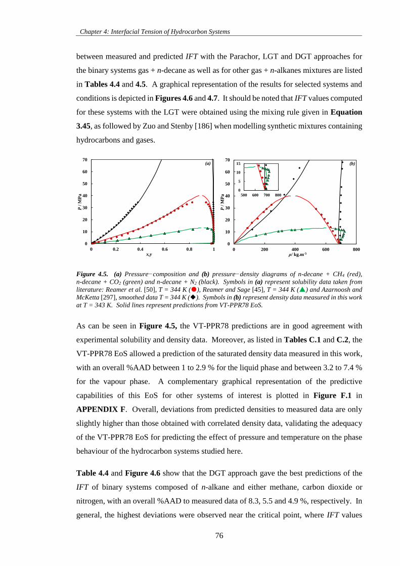
Chapter 4: Interfacial Tension of Hydrocarbon Systems
76
between measured and predicted IFT with the Parachor, LGT and DGT approaches for
the binary systems gas + n-decane as well as for other gas + n-alkanes mixtures are listed
in Tables 4.4 and 4.5. A graphical representation of the results for selected systems and
conditions is depicted in Figures 4.6 and 4.7. It should be noted that IFT values computed
for these systems with the LGT were obtained using the mixing rule given in Equation
3.45, as followed by Zuo and Stenby [186] when modelling synthetic mixtures containing
hydrocarbons and gases.
Figure 4.5. (a) Pressure−composition and (b) pressure−density diagrams of n-decane + CH4 (red),
n-decane + CO2 (green) and n-decane + N2 (black). Symbols in (a) represent solubility data taken from
literature: Reamer et al. [50], T = 344 K (), Reamer and Sage [45], T = 344 K () and Azarnoosh and
McKetta [297], smoothed data T = 344 K (). Symbols in (b) represent density data measured in this work
at T = 343 K. Solid lines represent predictions from VT-PPR78 EoS.
As can be seen in Figure 4.5, the VT-PPR78 predictions are in good agreement with
experimental solubility and density data. Moreover, as listed in Tables C.1 and C.2, the
VT-PPR78 EoS allowed a prediction of the saturated density data measured in this work,
with an overall %AAD between 1 to 2.9 % for the liquid phase and between 3.2 to 7.4 %
for the vapour phase. A complementary graphical representation of the predictive
capabilities of this EoS for other systems of interest is plotted in Figure F.1 in
APPENDIX F. Overall, deviations from predicted densities to measured data are only
slightly higher than those obtained with correlated density data, validating the adequacy
of the VT-PPR78 EoS for predicting the effect of pressure and temperature on the phase
behaviour of the hydrocarbon systems studied here.
Table 4.4 and Figure 4.6 show that the DGT approach gave the best predictions of the
IFT of binary systems composed of n-alkane and either methane, carbon dioxide or
nitrogen, with an overall %AAD to measured data of 8.3, 5.5 and 4.9 %, respectively. In
general, the highest deviations were observed near the critical point, where IFT values
0
10
20
30
40
50
60
70
0 200 400 600 800
P/
MP
a
ρ/ kg.m-3
0
10
20
30
40
50
60
70
0 0.2 0.4 0.6 0.8 1
P/
MP
a
x,y
0
5
10
15
500 600 700 800
(a) (b)
Chapter 4: Interfacial Tension of Hydrocarbon Systems
77
are rather low (IFT < 1.5 mN.m-1) and experimental uncertainties considerable. In this
region, the overall deviations of predictions with all models to measured data ranged
between 15.9 to 54.9 %. These discrepancies may be related to the inappropriate
description of the equilibrium properties by the selected phase behaviour model near the
critical point, as depicted in Figure 4.5 and F.1. In this sense, the computation of more
accurate interfacial tensions near critical point would require a refinement of the phase
behaviour model. The performance of the phase behaviour model near critical point can
be improved by the use of the crossover approach. In such approach, the transition from
classical to non-classical behaviour near the critical region is captured by a crossover
equation and thereby, the equilibrium properties in this region are successfully described.
The crossover approach was already incorporated to the PR78 EoS by others in previous
studies in literature [298,299]. However, this treatment requires the fitting of additional
parameters which characterise the critical region and thus, aiming at keeping the model
predictive, it was decided not to implement this approach here. All things considered, the
VT-PPR78 + DGT results are in good agreement with other DGT studies
[48,54,61,69,300] in which more complex and molecular-based equations of state, such
as SAFT and its derivatives, are used for the description the bulk saturated properties and
the Helmholtz free energy density of the fluid across the interfacial region.
It can be seen in Table 4.4 that the LGT model outperforms in general the Parachor
method for systems in methane and nitrogen atmospheres. Overall, the LGT allowed a
prediction of the IFT of CH4 + n-alkane and N2 + n-alkane systems far from the critical
point (i.e., IFT > 1.5 mN.m-1) with an overall %AAD of 10.1 and 7.7 %, respectively,
whereas deviations to measured data with the Parachor method were 14.5 and 13.9 %,
respectively. On the other hand, a significant underprediction of the IFT was obtained
for the systems containing carbon dioxide with the LGT at moderate pressures, as
depicted in Figure 4.6b, resulting in an overall %AAD of 20.3 %, whereas overall
deviations with the Parachor method yield only 9.3%. These findings are agreement with
the modelling results of Zuo and Stenby [186], in which a large and negative binary
interaction coefficient for the cross influence parameter was necessary for correct
description of the IFT of systems containing CO2 with the LGT model.
At this point it is important to note that the Parachor method can be shown to describe
correctly the IFT vs density difference behaviour near the critical point of pure
components [242]. However, the results obtained in this work with the Parachor method
Chapter 4: Interfacial Tension of Hydrocarbon Systems
78
for binary mixtures indicate a poor description of the IFT of such mixtures, with overall
%AADs higher than 23.8 % for IFT < 1.5 mN.m-1. On the one hand, these results can be
traced back to the inability of the phase behaviour model for describing the bulk
properties in this region. On the other hand, predictions with the Parachor are influenced
by the scaling exponent chosen i.e., by the value of E in Equation 3.2, which normally
ranges between 3.45 and 4. In the regime of low interfacial tension, lower exponents
seem often more suitable, whereas exponents approaching E = 4 (scaling exponent used
in this work) work better for intermediate and high interfacial tension [242]. The selection
of a scaling exponent E ≠ 4 would also require a recalculation of the Parachor values used
in this work (i.e., via Equation 3.3).
In line with what was described for the binary mixtures, Table 4.5 and Figure 4.7 show
that the largest deviations to experimental IFT data of the studied multicomponent
synthetic mixtures were also obtained with the LGT, in particular for MIX-2 and MIX-3
where CO2 is the predominant component, with an overall %AAD of 28.3% for IFT > 1.5
mN.m-1 and of 48.1% for IFT ≤ 1.5 mN.m-1. As depicted in Figure 4.7, the DGT
predictions are superior to that of the Parachor method, with the latter slightly
underpredicting the IFT of these systems. All in all, the DGT predictions for these
systems deviated from measured IFT data with an overall %AAD at moderate and high
pressures of 4.2 and 18.2 %, respectively, whereas the Parachor averaged deviations were
of 11.8 and 34.5 % in the same pressure range.
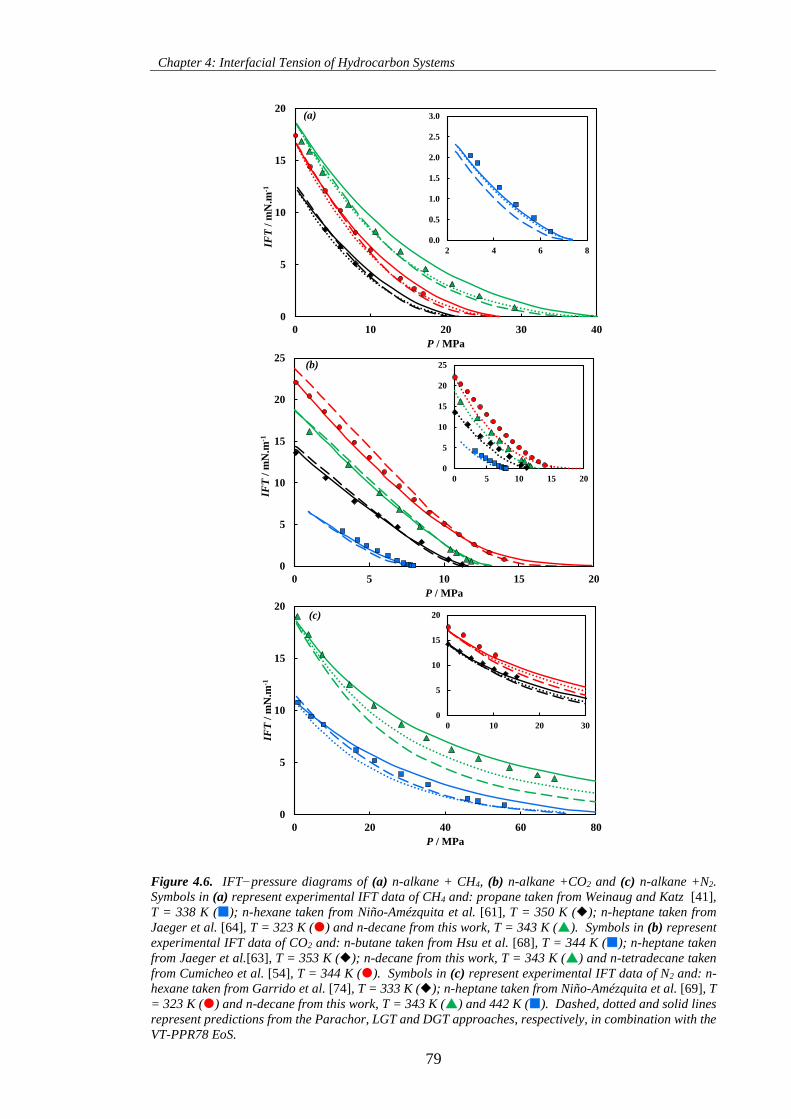
Chapter 4: Interfacial Tension of Hydrocarbon Systems
79
Figure 4.6. IFT−pressure diagrams of (a) n-alkane + CH4, (b) n-alkane +CO2 and (c) n-alkane +N2.
Symbols in (a) represent experimental IFT data of CH4 and: propane taken from Weinaug and Katz [41],
T = 338 K (); n-hexane taken from Niño-Amézquita et al. [61], T = 350 K (); n-heptane taken from
Jaeger et al. [64], T = 323 K () and n-decane from this work, T = 343 K (). Symbols in (b) represent
experimental IFT data of CO2 and: n-butane taken from Hsu et al. [68], T = 344 K (); n-heptane taken
from Jaeger et al.[63], T = 353 K (); n-decane from this work, T = 343 K () and n-tetradecane taken
from Cumicheo et al. [54], T = 344 K (). Symbols in (c) represent experimental IFT data of N2 and: n-
hexane taken from Garrido et al. [74], T = 333 K (); n-heptane taken from Niño-Amézquita et al. [69], T
= 323 K () and n-decane from this work, T = 343 K () and 442 K (). Dashed, dotted and solid lines
represent predictions from the Parachor, LGT and DGT approaches, respectively, in combination with the
VT-PPR78 EoS.
0
5
10
15
20
25
0 5 10 15 20
IFT
/ m
N.m
-1
P / MPa
0
5
10
15
20
25
0 5 10 15 20
0
5
10
15
20
0 10 20 30 40
IFT
/ m
N.m
-1
P / MPa
0.0
0.5
1.0
1.5
2.0
2.5
3.0
2 4 6 8
0
5
10
15
20
0 20 40 60 80
IFT
/ m
N.m
-1
P / MPa
0
5
10
15
20
0 10 20 30
(a)
(b)
(c)
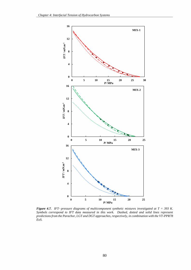
Chapter 4: Interfacial Tension of Hydrocarbon Systems
80
Figure 4.7. IFT−pressure diagrams of multicomponent synthetic mixtures investigated at T = 393 K.
Symbols correspond to IFT data measured in this work. Dashed, dotted and solid lines represent
predictions from the Parachor, LGT and DGT approaches, respectively, in combination with the VT-PPR78
EoS.
0
4
8
12
16
0 5 10 15 20 25 30
IFT
/ m
N.m
-1
P/ MPa
0
4
8
12
16
0 5 10 15 20 25
IFT
/ m
N.m
-1
P/ MPa
0
4
8
12
16
0 5 10 15 20 25
IFT
/ m
N.m
-1
P/ MPa
MIX-1
MIX-2
MIX-3
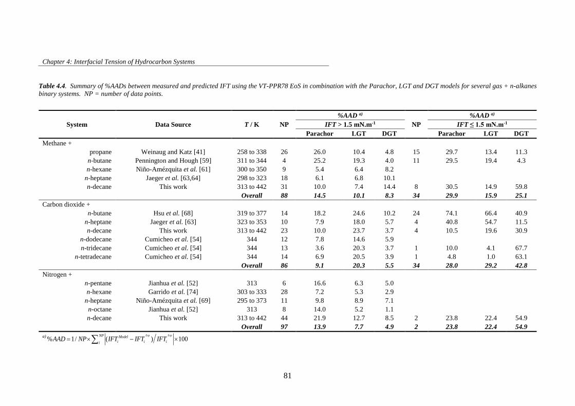
Chapter 4: Interfacial Tension of Hydrocarbon Systems
81
Table 4.4. Summary of %AADs between measured and predicted IFT using the VT-PPR78 EoS in combination with the Parachor, LGT and DGT models for several gas + n-alkanes
binary systems. NP = number of data points.
System
T / K NP
%AAD a)
NP
%AAD a)
Data Source IFT > 1.5 mN.m-1 IFT ≤ 1.5 mN.m-1
Parachor LGT DGT Parachor LGT DGT
Methane +
propane Weinaug and Katz [41] 258 to 338 26 26.0 10.4 4.8 15 29.7 13.4 11.3
n-butane Pennington and Hough [59] 311 to 344 4 25.2 19.3 4.0 11 29.5 19.4 4.3
n-hexane Niño-Amézquita et al. [61] 300 to 350 9 5.4 6.4 8.2
n-heptane Jaeger et al. [63,64] 298 to 323 18 6.1 6.8 10.1
n-decane This work 313 to 442 31 10.0 7.4 14.4 8 30.5 14.9 59.8
Overall 88 14.5 10.1 8.3 34 29.9 15.9 25.1
Carbon dioxide +
n-butane Hsu et al. [68] 319 to 377 14 18.2 24.6 10.2 24 74.1 66.4 40.9
n-heptane Jaeger et al. [63] 323 to 353 10 7.9 18.0 5.7 4 40.8 54.7 11.5
n-decane This work 313 to 442 23 10.0 23.7 3.7 4 10.5 19.6 30.9
n-dodecane Cumicheo et al. [54] 344 12 7.8 14.6 5.9
n-tridecane Cumicheo et al. [54] 344 13 3.6 20.3 3.7 1 10.0 4.1 67.7
n-tetradecane Cumicheo et al. [54] 344 14 6.9 20.5 3.9 1 4.8 1.0 63.1
Overall 86 9.1 20.3 5.5 34 28.0 29.2 42.8
Nitrogen +
n-pentane Jianhua et al. [52] 313 6 16.6 6.3 5.0
n-hexane Garrido et al. [74] 303 to 333 28 7.2 5.3 2.9
n-heptane Niño-Amézquita et al. [69] 295 to 373 11 9.8 8.9 7.1
n-octane Jianhua et al. [52] 313 8 14.0 5.2 1.1
n-decane This work 313 to 442 44 21.9 12.7 8.5 2 23.8 22.4 54.9
Overall 97 13.9 7.7 4.9 2 23.8 22.4 54.9
a)% 1/ ( ) 100
Exp ExpNP Model
i i iiAAD NP IFT IFT IFT
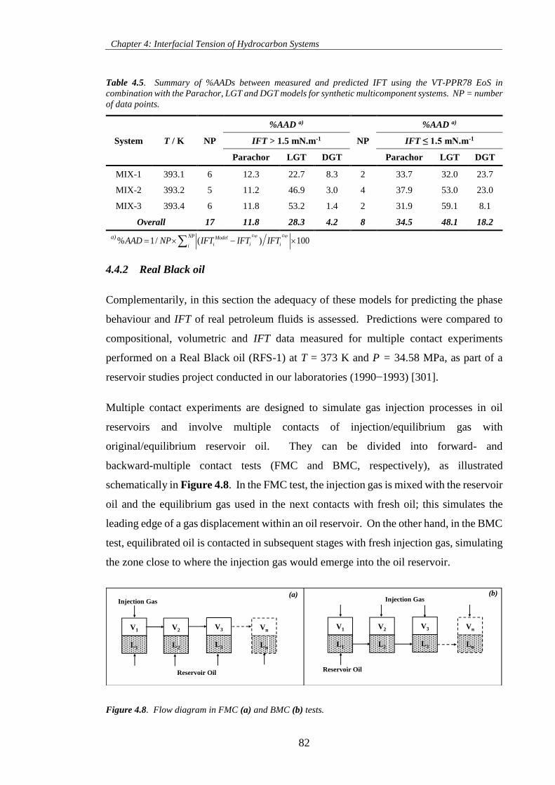
Chapter 4: Interfacial Tension of Hydrocarbon Systems
82
Table 4.5. Summary of %AADs between measured and predicted IFT using the VT-PPR78 EoS in
combination with the Parachor, LGT and DGT models for synthetic multicomponent systems. NP = number
of data points.
System T / K NP
%AAD a)
NP
%AAD a)
IFT > 1.5 mN.m-1 IFT ≤ 1.5 mN.m-1
Parachor LGT DGT Parachor LGT DGT
MIX-1 393.1 6 12.3 22.7 8.3 2 33.7 32.0 23.7
MIX-2 393.2 5 11.2 46.9 3.0 4 37.9 53.0 23.0
MIX-3 393.4 6 11.8 53.2 1.4 2 31.9 59.1 8.1
Overall 17 11.8 28.3 4.2 8 34.5 48.1 18.2
a)% 1/ ( ) 100
Exp ExpNP Model
i i iiAAD NP IFT IFT IFT
4.4.2 Real Black oil
Complementarily, in this section the adequacy of these models for predicting the phase
behaviour and IFT of real petroleum fluids is assessed. Predictions were compared to
compositional, volumetric and IFT data measured for multiple contact experiments
performed on a Real Black oil (RFS-1) at T = 373 K and P = 34.58 MPa, as part of a
reservoir studies project conducted in our laboratories (1990−1993) [301].
Multiple contact experiments are designed to simulate gas injection processes in oil
reservoirs and involve multiple contacts of injection/equilibrium gas with
original/equilibrium reservoir oil. They can be divided into forward- and
backward-multiple contact tests (FMC and BMC, respectively), as illustrated
schematically in Figure 4.8. In the FMC test, the injection gas is mixed with the reservoir
oil and the equilibrium gas used in the next contacts with fresh oil; this simulates the
leading edge of a gas displacement within an oil reservoir. On the other hand, in the BMC
test, equilibrated oil is contacted in subsequent stages with fresh injection gas, simulating
the zone close to where the injection gas would emerge into the oil reservoir.
Figure 4.8. Flow diagram in FMC (a) and BMC (b) tests.
Injection Gas
V1
L1
V2
L2
Vn
Ln
Reservoir Oil
V3
L3
Injection Gas
V1
L1
V2
L2
Vn
Ln
Reservoir Oil
V3
L3
(a) (b)
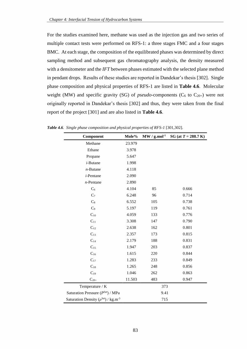
Chapter 4: Interfacial Tension of Hydrocarbon Systems
83
For the studies examined here, methane was used as the injection gas and two series of
multiple contact tests were performed on RFS-1: a three stages FMC and a four stages
BMC. At each stage, the composition of the equilibrated phases was determined by direct
sampling method and subsequent gas chromatography analysis, the density measured
with a densitometer and the IFT between phases estimated with the selected plane method
in pendant drops. Results of these studies are reported in Dandekar’s thesis [302]. Single
phase composition and physical properties of RFS-1 are listed in Table 4.6. Molecular
weight (MW) and specific gravity (SG) of pseudo-components (C6 to C20+) were not
originally reported in Dandekar’s thesis [302] and thus, they were taken from the final
report of the project [301] and are also listed in Table 4.6.
Table 4.6. Single phase composition and physical properties of RFS-1 [301,302].
Component Mole% MW / g.mol-1 SG (at T = 288.7 K)
Methane 23.979
Ethane 3.978
Propane 5.647
i-Butane 1.998
n-Butane 4.118
i-Pentane 2.090
n-Pentane 2.890
C6 4.104 85 0.666
C7 6.248 96 0.714
C8 6.552 105 0.738
C9 5.197 119 0.761
C10 4.059 133 0.776
C11 3.308 147 0.790
C12 2.638 162 0.801
C13 2.357 173 0.815
C14 2.179 188 0.831
C15 1.947 203 0.837
C16 1.615 220 0.844
C17 1.283 233 0.849
C18 1.265 248 0.856
C19 1.046 262 0.863
C20+ 11.503 483 0.947
Temperature / K 373
Saturation Pressure (PSat) / MPa 9.41
Saturation Density (ρSat) / kg.m-3 715
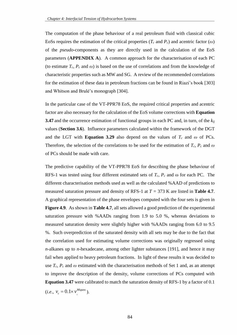
Chapter 4: Interfacial Tension of Hydrocarbon Systems
84
The computation of the phase behaviour of a real petroleum fluid with classical cubic
EoSs requires the estimation of the critical properties (Tc and Pc) and acentric factor (ω)
of the pseudo-components as they are directly used in the calculation of the EoS
parameters (APPENDIX A). A common approach for the characterisation of each PC
(to estimate Tc, Pc and ω) is based on the use of correlations and from the knowledge of
characteristic properties such as MW and SG. A review of the recommended correlations
for the estimation of these data in petroleum fractions can be found in Riazi’s book [303]
and Whitson and Brulé’s monograph [304].
In the particular case of the VT-PPR78 EoS, the required critical properties and acentric
factor are also necessary for the calculation of the EoS volume corrections with Equation
3.47 and the occurrence estimation of functional groups in each PC and, in turn, of the kij
values (Section 3.6). Influence parameters calculated within the framework of the DGT
and the LGT with Equation 3.29 also depend on the values of Tc and ω of PCs.
Therefore, the selection of the correlations to be used for the estimation of Tc, Pc and ω
of PCs should be made with care.
The predictive capability of the VT-PPR78 EoS for describing the phase behaviour of
RFS-1 was tested using four different estimated sets of Tc, Pc and ω for each PC. The
different characterisation methods used as well as the calculated %AAD of predictions to
measured saturation pressure and density of RFS-1 at T = 373 K are listed in Table 4.7.
A graphical representation of the phase envelopes computed with the four sets is given in
Figure 4.9. As shown in Table 4.7, all sets allowed a good prediction of the experimental
saturation pressure with %AADs ranging from 1.9 to 5.0 %, whereas deviations to
measured saturation density were slightly higher with %AADs ranging from 6.0 to 9.5
%. Such overprediction of the saturated density with all sets may be due to the fact that
the correlation used for estimating volume corrections was originally regressed using
n-alkanes up to n-hexadecane, among other lighter substances [191], and hence it may
fail when applied to heavy petroleum fractions. In light of these results it was decided to
use Tc, Pc and ω estimated with the characterisation methods of Set 1 and, as an attempt
to improve the description of the density, volume corrections of PCs computed with
Equation 3.47 were calibrated to match the saturation density of RFS-1 by a factor of 0.1
(i.e., 0.1c
Miqueu
cv v ).
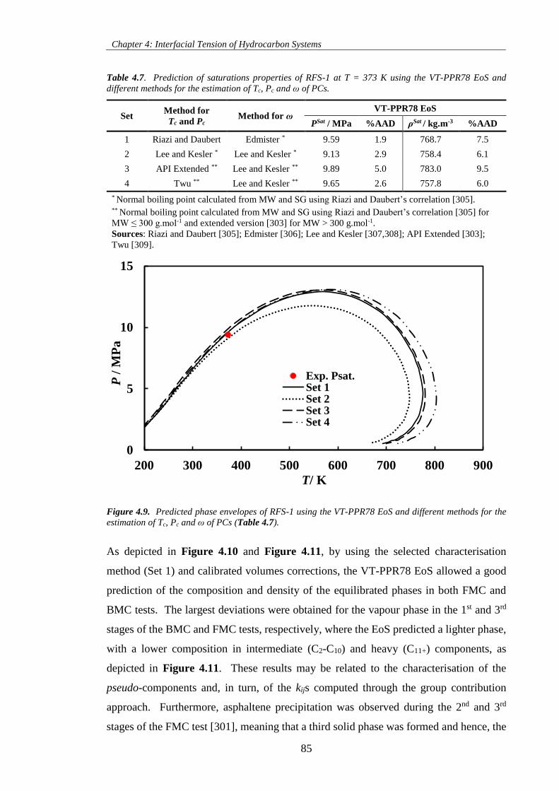
Chapter 4: Interfacial Tension of Hydrocarbon Systems
85
Table 4.7. Prediction of saturations properties of RFS-1 at T = 373 K using the VT-PPR78 EoS and
different methods for the estimation of Tc, Pc and ω of PCs.
Set Method for
Tc and Pc Method for ω
VT-PPR78 EoS
PSat / MPa %AAD ρSat / kg.m-3 %AAD
1 Riazi and Daubert Edmister * 9.59 1.9 768.7 7.5
2 Lee and Kesler * Lee and Kesler * 9.13 2.9 758.4 6.1
3 API Extended ** Lee and Kesler ** 9.89 5.0 783.0 9.5
4 Twu ** Lee and Kesler ** 9.65 2.6 757.8 6.0
* Normal boiling point calculated from MW and SG using Riazi and Daubert’s correlation [305]. ** Normal boiling point calculated from MW and SG using Riazi and Daubert’s correlation [305] for
MW ≤ 300 g.mol-1 and extended version [303] for MW > 300 g.mol-1.
Sources: Riazi and Daubert [305]; Edmister [306]; Lee and Kesler [307,308]; API Extended [303];
Twu [309].
Figure 4.9. Predicted phase envelopes of RFS-1 using the VT-PPR78 EoS and different methods for the
estimation of Tc, Pc and ω of PCs (Table 4.7).
As depicted in Figure 4.10 and Figure 4.11, by using the selected characterisation
method (Set 1) and calibrated volumes corrections, the VT-PPR78 EoS allowed a good
prediction of the composition and density of the equilibrated phases in both FMC and
BMC tests. The largest deviations were obtained for the vapour phase in the 1st and 3rd
stages of the BMC and FMC tests, respectively, where the EoS predicted a lighter phase,
with a lower composition in intermediate (C2-C10) and heavy (C11+) components, as
depicted in Figure 4.11. These results may be related to the characterisation of the
pseudo-components and, in turn, of the kijs computed through the group contribution
approach. Furthermore, asphaltene precipitation was observed during the 2nd and 3rd
stages of the FMC test [301], meaning that a third solid phase was formed and hence, the
0
5
10
15
200 300 400 500 600 700 800 900
P/
MP
a
T/ K
Exp. Psat.Set 1Set 2Set 3Set 4
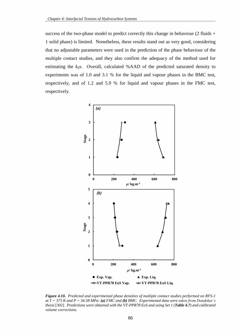
Chapter 4: Interfacial Tension of Hydrocarbon Systems
86
success of the two-phase model to predict correctly this change in behaviour (2 fluids +
1 solid phase) is limited. Nonetheless, these results stand out as very good, considering
that no adjustable parameters were used in the prediction of the phase behaviour of the
multiple contact studies, and they also confirm the adequacy of the method used for
estimating the kijs. Overall, calculated %AAD of the predicted saturated density to
experiments was of 1.0 and 3.1 % for the liquid and vapour phases in the BMC test,
respectively, and of 1.2 and 5.9 % for liquid and vapour phases in the FMC test,
respectively.
Figure 4.10. Predicted and experimental phase densities of multiple contact studies performed on RFS-1
at T = 373 K and P = 34.58 MPa: (a) FMC and (b) BMC. Experimental data were taken from Dandekar’s
thesis [302]. Predictions were obtained with the VT-PPR78 EoS and using Set 1 (Table 4.7) and calibrated
volume corrections.
0
1
2
3
4
0 200 400 600 800
Sta
ge
ρ/ kg.m-3
0
1
2
3
4
5
0 200 400 600 800
Sta
ge
ρ/ kg.m-3
Exp. Vap. Exp. Liq.
VT-PPR78 EoS Vap. VT-PPR78 EoS Liq.
(a)
(b)
Chapter 4: Interfacial Tension of Hydrocarbon Systems
87
Figure 4.11. Predicted and experimental phase compositions of multiple contact studies performed of
RFS-1 at T = 373 K and P = 34.58 MPa: (a) FMC and (b) BMC. Experimental data were taken from
Dandekar’s thesis [302]. Predictions were obtained with the VT-PPR78 EoS and using Set 1 (Table 4.7)
and calibrated volume corrections.
RFS-1
Exp. Vap. FMC
Exp. Liq. FMC
VT-PPR78 EoS Vap.
VT-PPR78 EoS Liq.
100 % C1
0 % C1
20%
30%
10%
40%
50%
60%
70%
80%
90%
RFS-1
Exp. Vap. BMC
Exp. Liq. BMC
VT-PPR78 EoS Vap.
VT-PPR78 EoS Liq.
100 % C1
0 % C1
20%
30%
10%
40%
50%
60%
70%
80%
90%
(a)
(b)
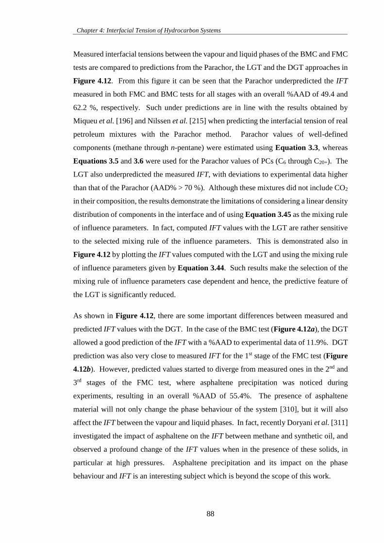
Chapter 4: Interfacial Tension of Hydrocarbon Systems
88
Measured interfacial tensions between the vapour and liquid phases of the BMC and FMC
tests are compared to predictions from the Parachor, the LGT and the DGT approaches in
Figure 4.12. From this figure it can be seen that the Parachor underpredicted the IFT
measured in both FMC and BMC tests for all stages with an overall %AAD of 49.4 and
62.2 %, respectively. Such under predictions are in line with the results obtained by
Miqueu et al. [196] and Nilssen et al. [215] when predicting the interfacial tension of real
petroleum mixtures with the Parachor method. Parachor values of well-defined
components (methane through n-pentane) were estimated using Equation 3.3, whereas
Equations 3.5 and 3.6 were used for the Parachor values of PCs (C6 through C20+). The
LGT also underpredicted the measured IFT, with deviations to experimental data higher
than that of the Parachor (AAD% > 70 %). Although these mixtures did not include CO2
in their composition, the results demonstrate the limitations of considering a linear density
distribution of components in the interface and of using Equation 3.45 as the mixing rule
of influence parameters. In fact, computed IFT values with the LGT are rather sensitive
to the selected mixing rule of the influence parameters. This is demonstrated also in
Figure 4.12 by plotting the IFT values computed with the LGT and using the mixing rule
of influence parameters given by Equation 3.44. Such results make the selection of the
mixing rule of influence parameters case dependent and hence, the predictive feature of
the LGT is significantly reduced.
As shown in Figure 4.12, there are some important differences between measured and
predicted IFT values with the DGT. In the case of the BMC test (Figure 4.12a), the DGT
allowed a good prediction of the IFT with a %AAD to experimental data of 11.9%. DGT
prediction was also very close to measured IFT for the 1st stage of the FMC test (Figure
4.12b). However, predicted values started to diverge from measured ones in the 2nd and
3rd stages of the FMC test, where asphaltene precipitation was noticed during
experiments, resulting in an overall %AAD of 55.4%. The presence of asphaltene
material will not only change the phase behaviour of the system [310], but it will also
affect the IFT between the vapour and liquid phases. In fact, recently Doryani et al. [311]
investigated the impact of asphaltene on the IFT between methane and synthetic oil, and
observed a profound change of the IFT values when in the presence of these solids, in
particular at high pressures. Asphaltene precipitation and its impact on the phase
behaviour and IFT is an interesting subject which is beyond the scope of this work.
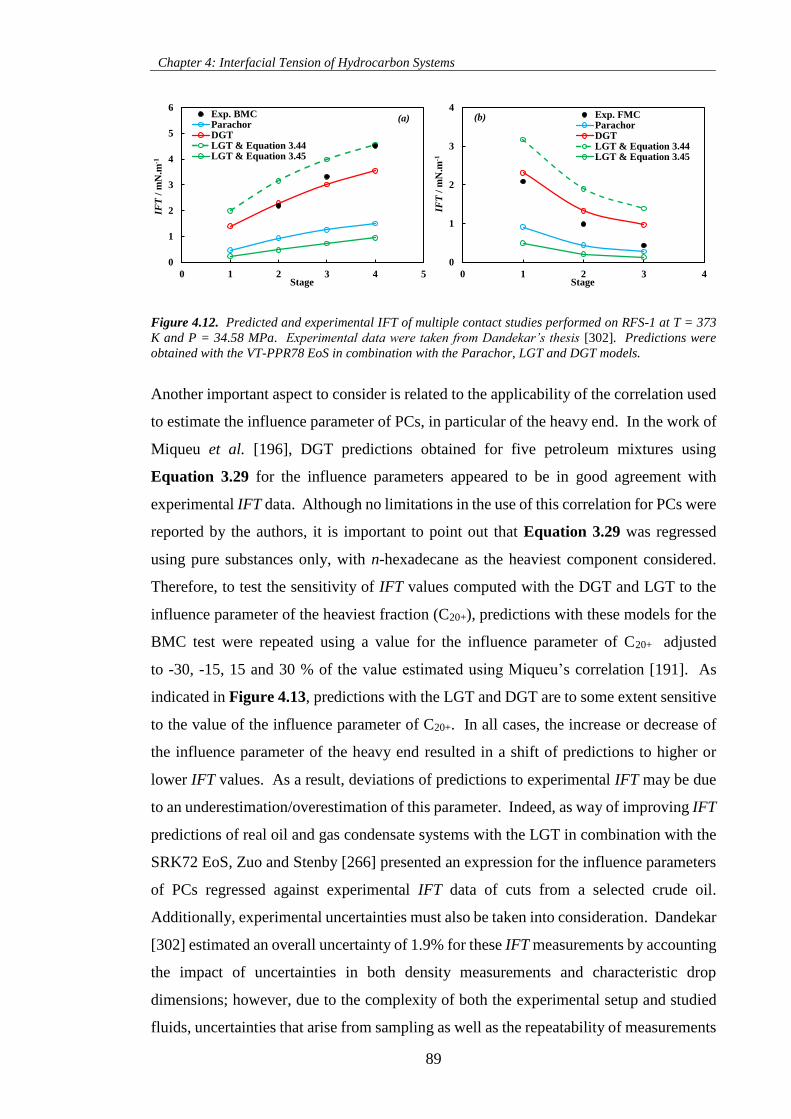
Chapter 4: Interfacial Tension of Hydrocarbon Systems
89
Figure 4.12. Predicted and experimental IFT of multiple contact studies performed on RFS-1 at T = 373
K and P = 34.58 MPa. Experimental data were taken from Dandekar’s thesis [302]. Predictions were
obtained with the VT-PPR78 EoS in combination with the Parachor, LGT and DGT models.
Another important aspect to consider is related to the applicability of the correlation used
to estimate the influence parameter of PCs, in particular of the heavy end. In the work of
Miqueu et al. [196], DGT predictions obtained for five petroleum mixtures using
Equation 3.29 for the influence parameters appeared to be in good agreement with
experimental IFT data. Although no limitations in the use of this correlation for PCs were
reported by the authors, it is important to point out that Equation 3.29 was regressed
using pure substances only, with n-hexadecane as the heaviest component considered.
Therefore, to test the sensitivity of IFT values computed with the DGT and LGT to the
influence parameter of the heaviest fraction (C20+), predictions with these models for the
BMC test were repeated using a value for the influence parameter of C20+ adjusted
to -30, -15, 15 and 30 % of the value estimated using Miqueu’s correlation [191]. As
indicated in Figure 4.13, predictions with the LGT and DGT are to some extent sensitive
to the value of the influence parameter of C20+. In all cases, the increase or decrease of
the influence parameter of the heavy end resulted in a shift of predictions to higher or
lower IFT values. As a result, deviations of predictions to experimental IFT may be due
to an underestimation/overestimation of this parameter. Indeed, as way of improving IFT
predictions of real oil and gas condensate systems with the LGT in combination with the
SRK72 EoS, Zuo and Stenby [266] presented an expression for the influence parameters
of PCs regressed against experimental IFT data of cuts from a selected crude oil.
Additionally, experimental uncertainties must also be taken into consideration. Dandekar
[302] estimated an overall uncertainty of 1.9% for these IFT measurements by accounting
the impact of uncertainties in both density measurements and characteristic drop
dimensions; however, due to the complexity of both the experimental setup and studied
fluids, uncertainties that arise from sampling as well as the repeatability of measurements
0
1
2
3
4
5
6
0 1 2 3 4 5
IFT
/ m
N.m
-1
Stage
Exp. BMCParachorDGTLGT & Equation 3.44LGT & Equation 3.45
0
1
2
3
4
0 1 2 3 4
IFT
/ m
N.m
-1
Stage
Exp. FMCParachorDGTLGT & Equation 3.44LGT & Equation 3.45
(a) (b)
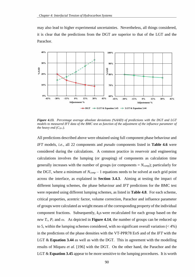
Chapter 4: Interfacial Tension of Hydrocarbon Systems
90
may also lead to higher experimental uncertainties. Nevertheless, all things considered,
it is clear that the predictions from the DGT are superior to that of the LGT and the
Parachor.
Figure 4.13. Percentage average absolute deviations (%AAD) of predictions with the DGT and LGT
models to measured IFT data of the BMC test as function of the adjustment of the influence parameter of
the heavy end (C20+).
All predictions described above were obtained using full component phase behaviour and
IFT models, i.e., all 22 components and pseudo components listed in Table 4.6 were
considered during the calculations. A common practice in reservoir and engineering
calculations involves the lumping (or grouping) of components as calculation time
generally increases with the number of groups (or components = Ncomp); particularly for
the DGT, where a minimum of Ncomp – 1 equations needs to be solved at each grid point
across the interface, as explained in Section 3.4.3. Aiming at testing the impact of
different lumping schemes, the phase behaviour and IFT predictions for the BMC test
were repeated using different lumping schemes, as listed in Table 4.8. For each scheme,
critical properties, acentric factor, volume correction, Parachor and influence parameter
of groups were calculated as weight means of the corresponding property of the individual
component fractions. Subsequently, kijs were recalculated for each group based on the
new Tc, Pc and ω. As depicted in Figure 4.14, the number of groups can be reduced up
to 5, within the lumping schemes considered, with no significant overall variation (< 4%)
in the predictions of the phase densities with the VT-PPR78 EoS and of the IFT with the
LGT & Equation 3.44 as well as with the DGT. This in agreement with the modelling
results of Miqueu et al. [196] with the DGT. On the other hand, the Parachor and the
LGT & Equation 3.45 appear to be more sensitive to the lumping procedures. It is worth
60%
70%
80%
90%
100%
-45% -30% -15% 0% 15% 30% 45%
%A
AD
Adjustement %
0%
10%
20%
30%
40%
-45% -30% -15% 0% 15% 30% 45%
%A
AD
Adjustement %
DGT LGT & Equation 3.45 LGT & Equation 3.44
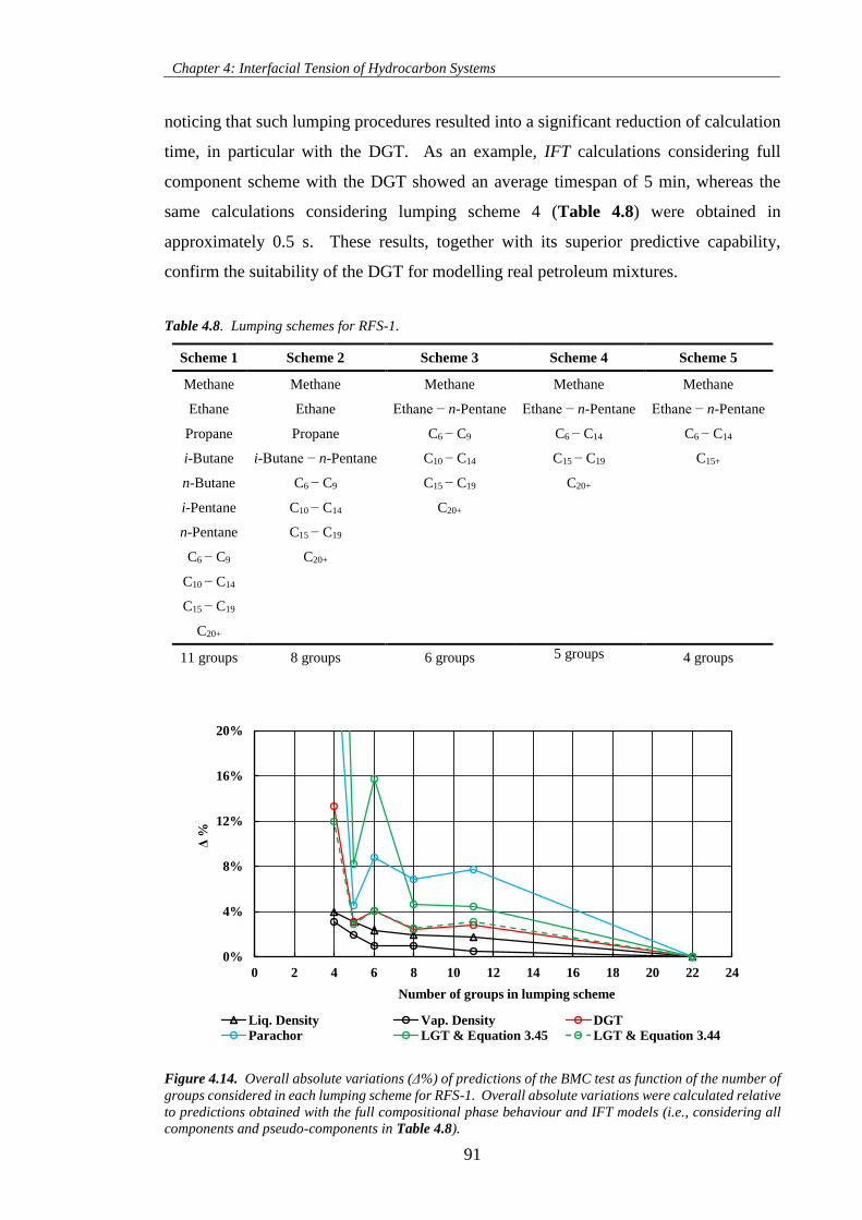
Chapter 4: Interfacial Tension of Hydrocarbon Systems
91
noticing that such lumping procedures resulted into a significant reduction of calculation
time, in particular with the DGT. As an example, IFT calculations considering full
component scheme with the DGT showed an average timespan of 5 min, whereas the
same calculations considering lumping scheme 4 (Table 4.8) were obtained in
approximately 0.5 s. These results, together with its superior predictive capability,
confirm the suitability of the DGT for modelling real petroleum mixtures.
Table 4.8. Lumping schemes for RFS-1.
Scheme 1 Scheme 2 Scheme 3 Scheme 4 Scheme 5
Methane Methane Methane Methane Methane
Ethane Ethane Ethane − n-Pentane Ethane − n-Pentane Ethane − n-Pentane
Propane Propane C6 − C9 C6 − C14 C6 − C14
i-Butane i-Butane − n-Pentane C10 − C14 C15 − C19 C15+
n-Butane C6 − C9 C15 − C19 C20+
i-Pentane C10 − C14 C20+
n-Pentane C15 − C19
C6 − C9 C20+
C10 − C14
C15 − C19
C20+
11 groups 8 groups 6 groups 5 groups 4 groups
Figure 4.14. Overall absolute variations (Δ%) of predictions of the BMC test as function of the number of
groups considered in each lumping scheme for RFS-1. Overall absolute variations were calculated relative
to predictions obtained with the full compositional phase behaviour and IFT models (i.e., considering all
components and pseudo-components in Table 4.8).
0%
4%
8%
12%
16%
20%
0 2 4 6 8 10 12 14 16 18 20 22 24
Δ%
Number of groups in lumping scheme
Liq. Density Vap. Density DGT
Parachor LGT & Equation 3.45 LGT & Equation 3.44
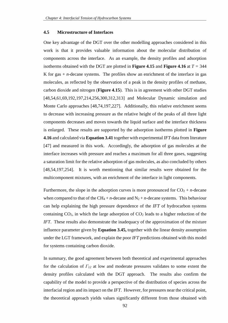
Chapter 4: Interfacial Tension of Hydrocarbon Systems
92
4.5 Microstructure of Interfaces
One key advantage of the DGT over the other modelling approaches considered in this
work is that it provides valuable information about the molecular distribution of
components across the interface. As an example, the density profiles and adsorption
isotherms obtained with the DGT are plotted in Figure 4.15 and Figure 4.16 at T = 344
K for gas + n-decane systems. The profiles show an enrichment of the interface in gas
molecules, as reflected by the observation of a peak in the density profiles of methane,
carbon dioxide and nitrogen (Figure 4.15). This is in agreement with other DGT studies
[48,54,61,69,192,197,214,256,300,312,313] and Molecular Dynamic simulation and
Monte Carlo approaches [48,74,197,227]. Additionally, this relative enrichment seems
to decrease with increasing pressure as the relative height of the peaks of all three light
components decreases and moves towards the liquid surface and the interface thickness
is enlarged. These results are supported by the adsorption isotherms plotted in Figure
4.16 and calculated via Equation 3.41 together with experimental IFT data from literature
[47] and measured in this work. Accordingly, the adsorption of gas molecules at the
interface increases with pressure and reaches a maximum for all three gases, suggesting
a saturation limit for the relative adsorption of gas molecules, as also concluded by others
[48,54,197,254]. It is worth mentioning that similar results were obtained for the
multicomponent mixtures, with an enrichment of the interface in light components.
Furthermore, the slope in the adsorption curves is more pronounced for CO2 + n-decane
when compared to that of the CH4 + n-decane and N2 + n-decane systems. This behaviour
can help explaining the high pressure dependence of the IFT of hydrocarbon systems
containing CO2, in which the large adsorption of CO2 leads to a higher reduction of the
IFT. These results also demonstrate the inadequacy of the approximation of the mixture
influence parameter given by Equation 3.45, together with the linear density assumption
under the LGT framework, and explain the poor IFT predictions obtained with this model
for systems containing carbon dioxide.
In summary, the good agreement between both theoretical and experimental approaches
for the calculation of Γ12 at low and moderate pressures validates to some extent the
density profiles calculated with the DGT approach. The results also confirm the
capability of the model to provide a perspective of the distribution of species across the
interfacial region and its impact on the IFT. However, for pressures near the critical point,
the theoretical approach yields values significantly different from those obtained with
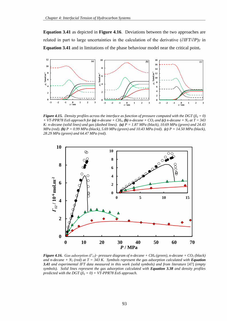
Chapter 4: Interfacial Tension of Hydrocarbon Systems
93
Equation 3.41 as depicted in Figure 4.16. Deviations between the two approaches are
related in part to large uncertainties in the calculation of the derivative (∂IFT/∂P)T in
Equation 3.41 and in limitations of the phase behaviour model near the critical point.
Figure 4.15. Density profiles across the interface as function of pressure computed with the DGT (βij = 0)
+ VT-PPR78 EoS approach for (a) n-decane + CH4, (b) n-decane + CO2 and (c) n-decane + N2 at T = 343
K: n-decane (solid lines) and gas (dashed lines). (a) P = 1.87 MPa (black), 10.69 MPa (green) and 24.43
MPa (red). (b) P = 0.99 MPa (black), 5.69 MPa (green) and 10.43 MPa (red). (c) P = 14.50 MPa (black),
28.29 MPa (green) and 64.47 MPa (red).
Figure 4.16. Gas adsorption (Γ12)−pressure diagram of n-decane + CH4 (green), n-decane + CO2 (black)
and n-decane + N2 (red) at T = 343 K. Symbols represent the gas adsorption calculated with Equation
3.41 and experimental IFT data measured in this work (solid symbols) and from literature [47] (empty
symbols). Solid lines represent the gas adsorption calculated with Equation 3.38 and density profiles
predicted with the DGT (βij = 0) + VT-PPR78 EoS approach.
0
2
4
6
8
10
-3 -2 -1 0 1 2 3
ρi/
km
ol.
m-3
z / nm
0
2
4
6
8
10
12
-3 -2 -1 0 1 2 3
ρi/
km
ol.
m-3
z / nm
0
2
4
6
8
10
12
14
16
18
-3 -2 -1 0 1 2 3
ρi/
km
ol.
m-3
z / nm
(a) (b) (c)
0
2
4
6
8
10
0 10 20 30 40 50 60 70
Γ1
2/
10
-6 m
ol.
m-2
P / MPa
0
2
4
6
8
10
0 5 10 15
Chapter 4: Interfacial Tension of Hydrocarbon Systems
94
4.6 Summary
Interfacial tension and saturated density data of three gas + n-decane binary mixtures as
well as of three multicomponent hydrocarbon systems have been measured over a broad
range of conditions (temperatures up to 442 K and pressures up to 69 MPa). Saturated
density data were correlated with the PR78 EoS and combined with measured capillary
constants to estimate the IFT of the studied systems. Measurements performed here for
the binary systems were found to be in good agreement with selected literature data,
validating both the methodology and the experimental procedure followed. The results
showed that generally the IFT decreased with increasing temperatures and pressures; a
crossover pressure region was observed between isotherms for the CO2 + n-decane
system. Moreover, for systems containing CO2, low interfacial values were achieved at
significantly lower pressures, readily showing that CO2 is an effective agent in the
reduction of interfacial forces and thus, in increasing oil recovery. Both density and IFT
measurements complement the experimental gap found in literature and extend these
measurements to reservoir conditions.
The coupling of the VT-PPR78 EoS with the Parachor, the LGT and the DGT approaches
was applied and their predictive capabilities evaluated by comparison with density and
IFT data measured in this work and from literature. The evaluated systems included
binary and multicomponent synthetic hydrocarbon systems as well as one real petroleum
fluid. The phase behaviour model showed very good capabilities for predicting the effect
of pressure and temperature on the equilibrium phase compositions and densities of the
hydrocarbon systems, considering that no adjustable parameters to mixtures were used.
The poorest predictions were obtained close to the critical region, where classical cubic
EoSs generally fail. Furthermore, some deviations were also observed between predicted
and measured phase behaviour data of the 2nd and 3rd stages of the forward multiple
contact test performed on the real petroleum fluid; asphaltene precipitation, noticed
during experiments, has been pointed out as the potential cause. In general, the best IFT
predictions were obtained with the DGT model with an overall %AAD between 4.9 and
8.3 % to data of binary systems, and between 1.4 and 8.3 % to multicomponent systems
data at low and moderate pressures (IFT > 1.5mN.m-1). In the case of the multiple contact
tests, the DGT allowed predictions of the IFT of the BMC test with a %AAD of 11.9%
to experimental data, whereas for the FMC test, a significant overprediction of the IFT
was obtained in the stages where precipitation of asphaltene occurred, resulting in a
Chapter 4: Interfacial Tension of Hydrocarbon Systems
95
%AAD of 55.4 %. Predictions with the LGT showed to be very sensitive to the selected
influence parameters mixing rule and, for systems with high content in CO2 the Parachor
method performed better than the LGT. For low interfacial tension values (IFT < 1.5
mN.m-1), all IFT models considered deviated significantly to measured data. This can be
attributed in part to the experimental uncertainties in this region, but also to the deviations
of the VT-PPR78 EoS to the bulk properties of the equilibrium phases. Lastly, an
investigation of the impact of different grouping schemes showed that phase behaviour
and IFT predictions of the BMC test with the VT-PPR78 EoS + DGT approach remained
practically unaffected when five or more groups were used in the fluid description. The
use of such lumping schemes resulted in a significant reduction of the computation time,
specifically for the DGT, which makes this model a good candidate for industrial
applications and reservoir engineering calculations.
The DGT, through the calculation of the distribution of components in the interfacial
region, showed a local enrichment and relative adsorption of gas molecules in the
interfacial region, which increased with pressure and reached a saturation limit. This
behaviour was more pronounced for CO2 which seems to explain the high pressure
dependence of the IFT values of CO2 + n-alkane systems when compared to that of N2 +
n-alkane and CH4 + n-alkane systems. These results may also explain the large negative
deviations obtained with the LGT for systems with CO2, in which the assumption of a
linear density distribution of components in the interfacial region proved inadequate.
This show the need for adjusting binary interaction coefficients within the LGT
framework as a way of improving computed IFT values. Altogether, the good agreement
observed between calculated and experimental Gibbs adsorption isotherms confirms the
adequacy of the DGT for describing the complex microstructures that arise from fluid
interfaces and their impact on the IFT values.
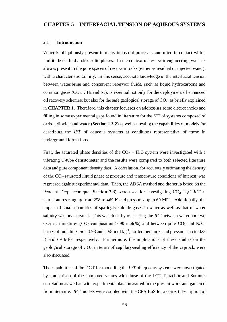
96
CHAPTER 5 – INTERFACIAL TENSION OF AQUEOUS SYSTEMS
5.1 Introduction
Water is ubiquitously present in many industrial processes and often in contact with a
multitude of fluid and/or solid phases. In the context of reservoir engineering, water is
always present in the pore spaces of reservoir rocks (either as residual or injected water),
with a characteristic salinity. In this sense, accurate knowledge of the interfacial tension
between water/brine and concurrent reservoir fluids, such as liquid hydrocarbons and
common gases (CO2, CH4 and N2), is essential not only for the deployment of enhanced
oil recovery schemes, but also for the safe geological storage of CO2, as briefly explained
in CHAPTER 1. Therefore, this chapter focusses on addressing some discrepancies and
filling in some experimental gaps found in literature for the IFT of systems composed of
carbon dioxide and water (Section 1.3.2) as well as testing the capabilities of models for
describing the IFT of aqueous systems at conditions representative of those in
underground formations.
First, the saturated phase densities of the CO2 + H2O system were investigated with a
vibrating U-tube densitometer and the results were compared to both selected literature
data and pure component density data. A correlation, for accurately estimating the density
of the CO2-saturated liquid phase at pressure and temperature conditions of interest, was
regressed against experimental data. Then, the ADSA method and the setup based on the
Pendant Drop technique (Section 2.3) were used for investigating CO2−H2O IFT at
temperatures ranging from 298 to 469 K and pressures up to 69 MPa. Additionally, the
impact of small quantities of sparingly soluble gases in water as well as that of water
salinity was investigated. This was done by measuring the IFT between water and two
CO2-rich mixtures (CO2 composition > 90 mole%) and between pure CO2 and NaCl
brines of molalities m = 0.98 and 1.98 mol.kg-1, for temperatures and pressures up to 423
K and 69 MPa, respectively. Furthermore, the implications of these studies on the
geological storage of CO2, in terms of capillary-sealing efficiency of the caprock, were
also discussed.
The capabilities of the DGT for modelling the IFT of aqueous systems were investigated
by comparison of the computed values with those of the LGT, Parachor and Sutton’s
correlation as well as with experimental data measured in the present work and gathered
from literature. IFT models were coupled with the CPA EoS for a correct description of
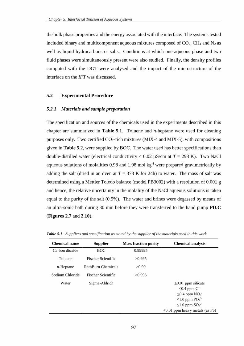
Chapter 5: Interfacial Tension of Aqueous Systems
97
the bulk phase properties and the energy associated with the interface. The systems tested
included binary and multicomponent aqueous mixtures composed of CO2, CH4 and N2 as
well as liquid hydrocarbons or salts. Conditions at which one aqueous phase and two
fluid phases were simultaneously present were also studied. Finally, the density profiles
computed with the DGT were analysed and the impact of the microstructure of the
interface on the IFT was discussed.
5.2 Experimental Procedure
5.2.1 Materials and sample preparation
The specification and sources of the chemicals used in the experiments described in this
chapter are summarized in Table 5.1. Toluene and n-heptane were used for cleaning
purposes only. Two certified CO2-rich mixtures (MIX-4 and MIX-5), with compositions
given in Table 5.2, were supplied by BOC. The water used has better specifications than
double-distilled water (electrical conductivity < 0.02 µS/cm at T = 298 K). Two NaCl
aqueous solutions of molalities 0.98 and 1.98 mol.kg-1 were prepared gravimetrically by
adding the salt (dried in an oven at T = 373 K for 24h) to water. The mass of salt was
determined using a Mettler Toledo balance (model PB3002) with a resolution of 0.001 g
and hence, the relative uncertainty in the molality of the NaCl aqueous solutions is taken
equal to the purity of the salt (0.5%). The water and brines were degassed by means of
an ultra-sonic bath during 30 min before they were transferred to the hand pump PD.C
(Figures 2.7 and 2.10).
Table 5.1. Suppliers and specification as stated by the supplier of the materials used in this work.
Chemical name Supplier Mass fraction purity Chemical analysis
Carbon dioxide BOC 0.99995
Toluene Fischer Scientific >0.995
n-Heptane RathBurn Chemicals >0.99
Sodium Chloride Fischer Scientific >0.995
Water Sigma-Aldrich ≤0.01 ppm silicate
≤0.4 ppm Cl-
≤0.4 ppm NO3-
≤1.0 ppm PO43-
≤1.0 ppm SO42-
≤0.01 ppm heavy metals (as Pb)
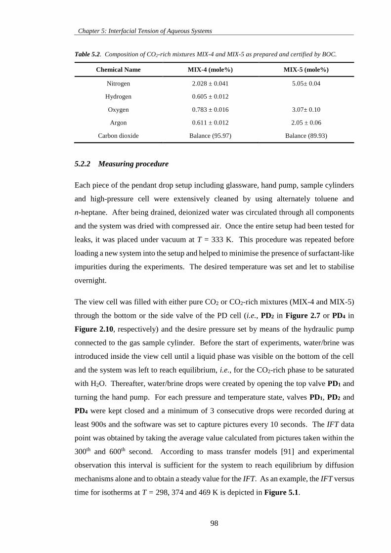
Chapter 5: Interfacial Tension of Aqueous Systems
98
Table 5.2. Composition of CO2-rich mixtures MIX-4 and MIX-5 as prepared and certified by BOC.
Chemical Name MIX-4 (mole%) MIX-5 (mole%)
Nitrogen 2.028 ± 0.041 5.05± 0.04
Hydrogen 0.605 ± 0.012
Oxygen 0.783 ± 0.016 3.07± 0.10
Argon 0.611 ± 0.012 2.05 ± 0.06
Carbon dioxide Balance (95.97) Balance (89.93)
5.2.2 Measuring procedure
Each piece of the pendant drop setup including glassware, hand pump, sample cylinders
and high-pressure cell were extensively cleaned by using alternately toluene and
n-heptane. After being drained, deionized water was circulated through all components
and the system was dried with compressed air. Once the entire setup had been tested for
leaks, it was placed under vacuum at T = 333 K. This procedure was repeated before
loading a new system into the setup and helped to minimise the presence of surfactant-like
impurities during the experiments. The desired temperature was set and let to stabilise
overnight.
The view cell was filled with either pure CO2 or CO2-rich mixtures (MIX-4 and MIX-5)
through the bottom or the side valve of the PD cell (i.e., PD2 in Figure 2.7 or PD4 in
Figure 2.10, respectively) and the desire pressure set by means of the hydraulic pump
connected to the gas sample cylinder. Before the start of experiments, water/brine was
introduced inside the view cell until a liquid phase was visible on the bottom of the cell
and the system was left to reach equilibrium, i.e., for the CO2-rich phase to be saturated
with H2O. Thereafter, water/brine drops were created by opening the top valve PD1 and
turning the hand pump. For each pressure and temperature state, valves PD1, PD2 and
PD4 were kept closed and a minimum of 3 consecutive drops were recorded during at
least 900s and the software was set to capture pictures every 10 seconds. The IFT data
point was obtained by taking the average value calculated from pictures taken within the
300th and 600th second. According to mass transfer models [91] and experimental
observation this interval is sufficient for the system to reach equilibrium by diffusion
mechanisms alone and to obtain a steady value for the IFT. As an example, the IFT versus
time for isotherms at T = 298, 374 and 469 K is depicted in Figure 5.1.
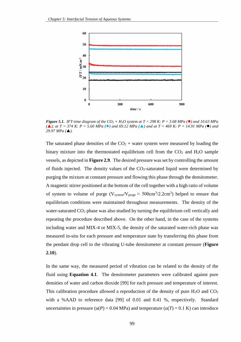
Chapter 5: Interfacial Tension of Aqueous Systems
99
Figure 5.1. IFT-time diagram of the CO2 + H2O system at T = 298 K: P = 3.68 MPa () and 10.63 MPa
(); at T = 374 K: P = 5.60 MPa () and 69.12 MPa () and at T = 469 K: P = 14.91 MPa () and
29.97 MPa ().
The saturated phase densities of the CO2 + water system were measured by loading the
binary mixture into the thermostated equilibrium cell from the CO2 and H2O sample
vessels, as depicted in Figure 2.9. The desired pressure was set by controlling the amount
of fluids injected. The density values of the CO2-saturated liquid were determined by
purging the mixture at constant pressure and flowing this phase through the densitometer.
A magnetic stirrer positioned at the bottom of the cell together with a high ratio of volume
of system to volume of purge (Vsystem/Vpurge ≈ 500cm3/2.2cm3) helped to ensure that
equilibrium conditions were maintained throughout measurements. The density of the
water-saturated CO2 phase was also studied by turning the equilibrium cell vertically and
repeating the procedure described above. On the other hand, in the case of the systems
including water and MIX-4 or MIX-5, the density of the saturated water-rich phase was
measured in-situ for each pressure and temperature state by transferring this phase from
the pendant drop cell to the vibrating U-tube densitometer at constant pressure (Figure
2.10).
In the same way, the measured period of vibration can be related to the density of the
fluid using Equation 4.1. The densitometer parameters were calibrated against pure
densities of water and carbon dioxide [99] for each pressure and temperature of interest.
This calibration procedure allowed a reproduction of the density of pure H2O and CO2
with a %AAD to reference data [99] of 0.01 and 0.41 %, respectively. Standard
uncertainties in pressure (u(P) = 0.04 MPa) and temperature (u(T) = 0.1 K) can introduce
0
10
20
30
40
50
60
0 300 600 900
IFT
/ m
N.m
-1
time / s
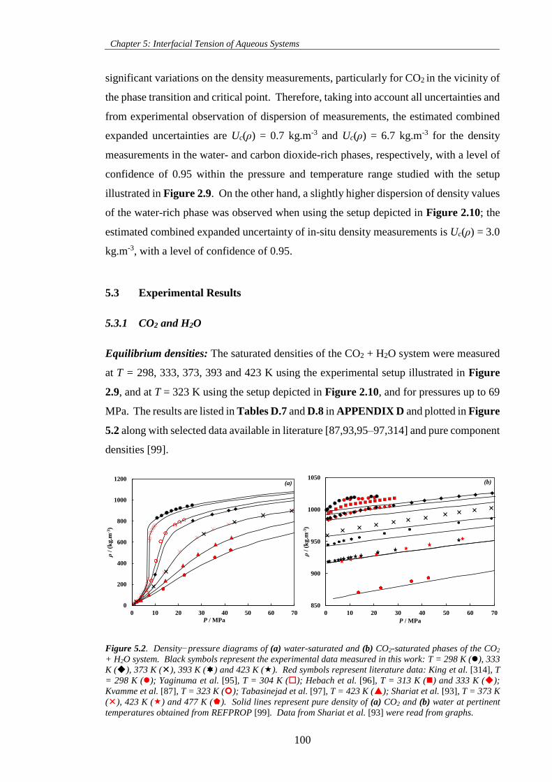
Chapter 5: Interfacial Tension of Aqueous Systems
100
significant variations on the density measurements, particularly for CO2 in the vicinity of
the phase transition and critical point. Therefore, taking into account all uncertainties and
from experimental observation of dispersion of measurements, the estimated combined
expanded uncertainties are Uc(ρ) = 0.7 kg.m-3 and Uc(ρ) = 6.7 kg.m-3 for the density
measurements in the water- and carbon dioxide-rich phases, respectively, with a level of
confidence of 0.95 within the pressure and temperature range studied with the setup
illustrated in Figure 2.9. On the other hand, a slightly higher dispersion of density values
of the water-rich phase was observed when using the setup depicted in Figure 2.10; the
estimated combined expanded uncertainty of in-situ density measurements is Uc(ρ) = 3.0
kg.m-3, with a level of confidence of 0.95.
5.3 Experimental Results
5.3.1 CO2 and H2O
Equilibrium densities: The saturated densities of the CO2 + H2O system were measured
at T = 298, 333, 373, 393 and 423 K using the experimental setup illustrated in Figure
2.9, and at T = 323 K using the setup depicted in Figure 2.10, and for pressures up to 69
MPa. The results are listed in Tables D.7 and D.8 in APPENDIX D and plotted in Figure
5.2 along with selected data available in literature [87,93,95–97,314] and pure component
densities [99].
Figure 5.2. Density−pressure diagrams of (a) water-saturated and (b) CO2-saturated phases of the CO2
+ H2O system. Black symbols represent the experimental data measured in this work: T = 298 K (), 333
K (), 373 K (), 393 K () and 423 K (). Red symbols represent literature data: King et al. [314], T
= 298 K (); Yaginuma et al. [95], T = 304 K (); Hebach et al. [96], T = 313 K () and 333 K ();
Kvamme et al. [87], T = 323 K (); Tabasinejad et al. [97], T = 423 K (); Shariat et al. [93], T = 373 K
(), 423 K () and 477 K (). Solid lines represent pure density of (a) CO2 and (b) water at pertinent
temperatures obtained from REFPROP [99]. Data from Shariat et al. [93] were read from graphs.
850
900
950
1000
1050
0 10 20 30 40 50 60 70
ρ/
(kg.m
-3)
P / MPa
0
200
400
600
800
1000
1200
0 10 20 30 40 50 60 70
ρ/
(kg.m
-3)
P / MPa
(a) (b)
Chapter 5: Interfacial Tension of Aqueous Systems
101
As can be seen in Figure 5.2, for all isotherms the density of the water-saturated CO2
phase is very close to that of pure CO2 within the experimental uncertainty. This is also
in agreement with what was already reported by several authors in literature
[7,87,93,96,97,314] and hence, the density of this phase can be fairly approximated to
that of pure CO2 [99]. On the other hand, the increase in density of the CO2-saturated
water phase with pressure exceeds that of pure water for all isotherms investigated and it
is in good agreement with the data gathered from open literature [93,96,97,314]. This
increase can be divided into two regions: whether CO2 is gaseous or
liquefied/supercritical. The density increase in the CO2-saturated water phases is more
pronounced when in contact with gaseous CO2 and moderate for liquefied/supercritical
CO2, and must be associated with the well-known decrease in solubility of CO2 molecules
in the water-rich phase [315]. The deviation between the pure and measured
CO2-saturated water densities is larger at low temperatures and high pressures, with a
maximum relative density difference of 1.7% (17 kg.m-3) obtained at T = 298.5 K and P
= 11.89 MPa.
Despite the overall low relative deviation observed between the pure and CO2-saturated
water densities in Figure 5.2, the density approximation of this phase to that of pure water
can result in significantly different overall density difference (i.e., Δρ) between the two
equilibrated fluids for interfacial tension estimations (Equation 2.9). In particular, this
is the case close to the density inversion conditions where the lowest values for Δρ are
obtained. The approximation of the density of the CO2-saturated water phase to that of
pure water would result in lower values for Δρ and therefore, in an underestimation of the
IFT values. This behaviour has also been reported by Chiquet et al. [7] who estimated a
Δρ up to 1.7 times smaller than the one obtained from experiments when pure density
assumption for the equilibrated phases is used at T = 308 K and P = 45 MPa.
In order to estimate the density of the CO2-saturated water phase at pertinent experimental
conditions, the correlation proposed by Hebach et al. [96] was extended in this work to
higher temperatures and pressures by using saturated phase density data measured here
and available in literature, as listed in Table 5.3. Accordingly, this correlation is
expressed as follows:
2
2 2 3 2 2
0 1 2 3 4 5 6 7 8
Correlation
H O a a P a T a P a T a TP a P a T P a P T 5.1
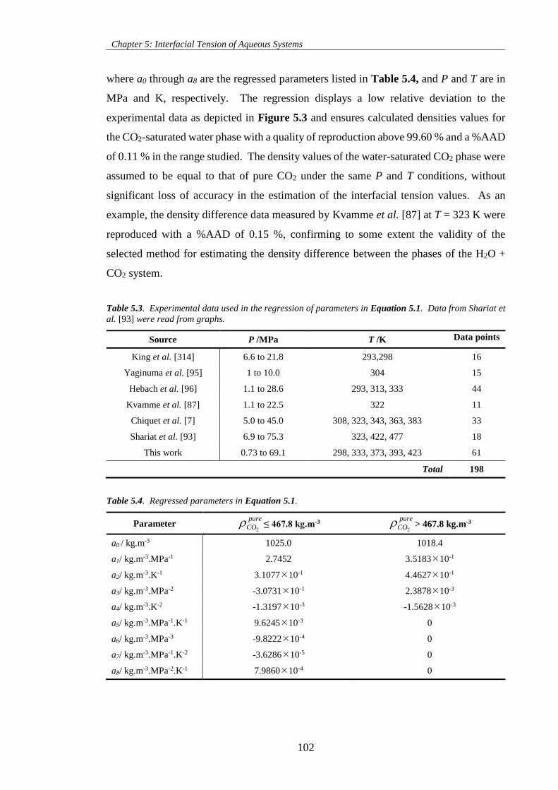
Chapter 5: Interfacial Tension of Aqueous Systems
102
where a0 through a8 are the regressed parameters listed in Table 5.4, and P and T are in
MPa and K, respectively. The regression displays a low relative deviation to the
experimental data as depicted in Figure 5.3 and ensures calculated densities values for
the CO2-saturated water phase with a quality of reproduction above 99.60 % and a %AAD
of 0.11 % in the range studied. The density values of the water-saturated CO2 phase were
assumed to be equal to that of pure CO2 under the same P and T conditions, without
significant loss of accuracy in the estimation of the interfacial tension values. As an
example, the density difference data measured by Kvamme et al. [87] at T = 323 K were
reproduced with a %AAD of 0.15 %, confirming to some extent the validity of the
selected method for estimating the density difference between the phases of the H2O +
CO2 system.
Table 5.3. Experimental data used in the regression of parameters in Equation 5.1. Data from Shariat et
al. [93] were read from graphs.
Source P /MPa T /K Data points
King et al. [314] 6.6 to 21.8 293,298 16
Yaginuma et al. [95] 1 to 10.0 304 15
Hebach et al. [96] 1.1 to 28.6 293, 313, 333 44
Kvamme et al. [87] 1.1 to 22.5 322 11
Chiquet et al. [7] 5.0 to 45.0 308, 323, 343, 363, 383 33
Shariat et al. [93] 6.9 to 75.3 323, 422, 477 18
This work 0.73 to 69.1 298, 333, 373, 393, 423 61
Total 198
Table 5.4. Regressed parameters in Equation 5.1.
Parameter 2
pure
CO ≤ 467.8 kg.m-3 2
pure
CO > 467.8 kg.m-3
a0 / kg.m-3 1025.0 1018.4
a1/ kg.m-3.MPa-1 2.7452 3.518310-1
a2/ kg.m-3.K-1 3.107710-1 4.462710-1
a3/ kg.m-3.MPa-2 -3.073110-1 2.387810-3
a4/ kg.m-3.K-2 -1.319710-3 -1.562810-3
a5/ kg.m-3.MPa-1.K-1 9.624510-3 0
a6/ kg.m-3.MPa-3 -9.822210-4 0
a7/ kg.m-3.MPa-1.K-2 -3.628610-5 0
a8/ kg.m-3.MPa-2.K-1 7.986010-4 0
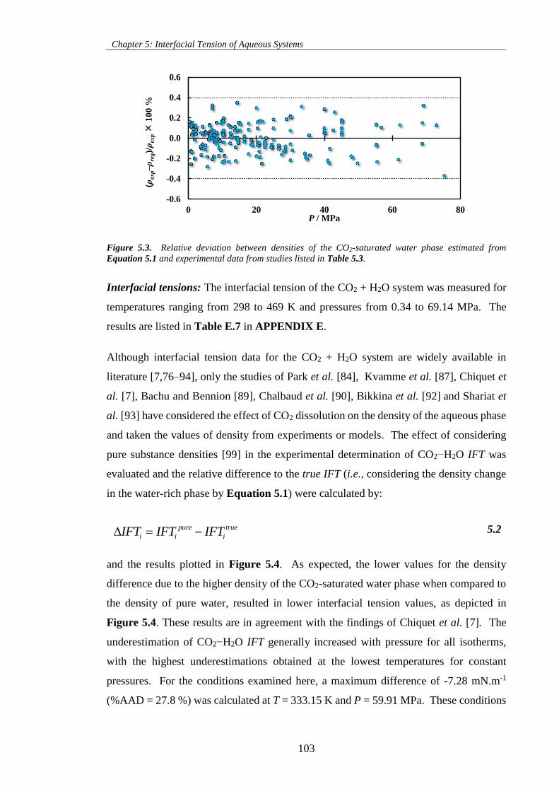
Chapter 5: Interfacial Tension of Aqueous Systems
103
Figure 5.3. Relative deviation between densities of the CO2-saturated water phase estimated from
Equation 5.1 and experimental data from studies listed in Table 5.3.
Interfacial tensions: The interfacial tension of the CO2 + H2O system was measured for
temperatures ranging from 298 to 469 K and pressures from 0.34 to 69.14 MPa. The
results are listed in Table E.7 in APPENDIX E.
Although interfacial tension data for the CO2 + H2O system are widely available in
literature [7,76–94], only the studies of Park et al. [84], Kvamme et al. [87], Chiquet et
al. [7], Bachu and Bennion [89], Chalbaud et al. [90], Bikkina et al. [92] and Shariat et
al. [93] have considered the effect of CO2 dissolution on the density of the aqueous phase
and taken the values of density from experiments or models. The effect of considering
pure substance densities [99] in the experimental determination of CO2−H2O IFT was
evaluated and the relative difference to the true IFT (i.e., considering the density change
in the water-rich phase by Equation 5.1) were calculated by:
pure true
i i iIFT IFT IFT 5.2
and the results plotted in Figure 5.4. As expected, the lower values for the density
difference due to the higher density of the CO2-saturated water phase when compared to
the density of pure water, resulted in lower interfacial tension values, as depicted in
Figure 5.4. These results are in agreement with the findings of Chiquet et al. [7]. The
underestimation of CO2−H2O IFT generally increased with pressure for all isotherms,
with the highest underestimations obtained at the lowest temperatures for constant
pressures. For the conditions examined here, a maximum difference of -7.28 mN.m-1
(%AAD = 27.8 %) was calculated at T = 333.15 K and P = 59.91 MPa. These conditions
-0.6
-0.4
-0.2
0.0
0.2
0.4
0.6
0 20 40 60 80
(ρex
p–
ρre
g)/
ρex
p
10
0 %
P / MPa
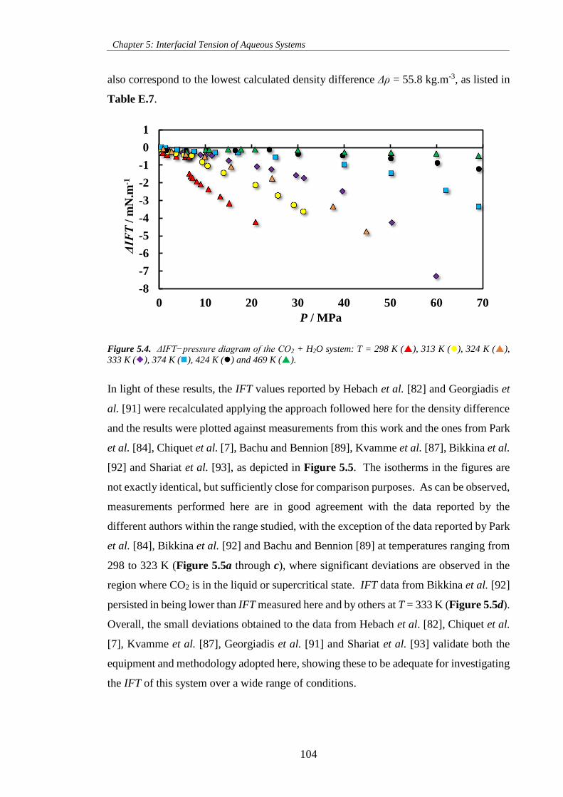
Chapter 5: Interfacial Tension of Aqueous Systems
104
also correspond to the lowest calculated density difference Δρ = 55.8 kg.m-3, as listed in
Table E.7.
Figure 5.4. ΔIFT−pressure diagram of the CO2 + H2O system: T = 298 K (), 313 K (), 324 K (),
333 K (), 374 K (), 424 K () and 469 K ().
In light of these results, the IFT values reported by Hebach et al. [82] and Georgiadis et
al. [91] were recalculated applying the approach followed here for the density difference
and the results were plotted against measurements from this work and the ones from Park
et al. [84], Chiquet et al. [7], Bachu and Bennion [89], Kvamme et al. [87], Bikkina et al.
[92] and Shariat et al. [93], as depicted in Figure 5.5. The isotherms in the figures are
not exactly identical, but sufficiently close for comparison purposes. As can be observed,
measurements performed here are in good agreement with the data reported by the
different authors within the range studied, with the exception of the data reported by Park
et al. [84], Bikkina et al. [92] and Bachu and Bennion [89] at temperatures ranging from
298 to 323 K (Figure 5.5a through c), where significant deviations are observed in the
region where CO2 is in the liquid or supercritical state. IFT data from Bikkina et al. [92]
persisted in being lower than IFT measured here and by others at T = 333 K (Figure 5.5d).
Overall, the small deviations obtained to the data from Hebach et al. [82], Chiquet et al.
[7], Kvamme et al. [87], Georgiadis et al. [91] and Shariat et al. [93] validate both the
equipment and methodology adopted here, showing these to be adequate for investigating
the IFT of this system over a wide range of conditions.
-8
-7
-6
-5
-4
-3
-2
-1
0
1
0 10 20 30 40 50 60 70
ΔIF
T/
mN
.m-1
P / MPa
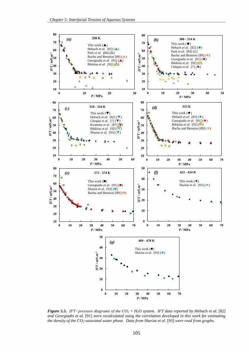
Chapter 5: Interfacial Tension of Aqueous Systems
105
Figure 5.5. IFT−pressure diagrams of the CO2 + H2O system. IFT data reported by Hebach et al. [82]
and Georgiadis et al. [91] were recalculated using the correlation developed in this work for estimating
the density of the CO2-saturated water phase. Data from Shariat et al. [93] were read from graphs.
10
20
30
40
50
60
70
80
0 10 20 30 40 50 60
IFT
/ m
N.m
-1
P / MPa
10
20
30
40
50
60
70
80
0 10 20 30 40 50 60 70
IFT
/ m
N.m
-1
P / MPa
10
20
30
40
50
60
70
80
0 10 20 30 40 50 60 70
IFT
/ m
N.m
-1
P / MPa
10
20
30
40
50
60
70
80
0 10 20 30
IFT
/ m
N.m
-1
P / MPa
0
10
20
30
40
50
0 10 20 30 40 50 60 70
IFT
/ m
N.m
-1
P / MPa
10
20
30
40
50
60
70
80
0 10 20 30 40 50
IFT
/ m
N.m
-1
P / MPa
0
10
20
30
40
50
0 10 20 30 40 50 60 70
IFT
/ m
N.m
-1
P / MPa
298 K 308 - 314 K
318 - 324 K 333 K
373 - 374 K 422 - 424 K
469 - 478 K
This work ()
Hebach et al. [82] ()
Park et al. [84] ( )
Bachu and Bennion [89] () Georgiadis et al. [91] ()
Bikkina et al. [92] ( )
This work () Hebach et al. [82] ()
Park et al. [84] ( )
Bachu and Bennion [89] () Georgiadis et al. [91] ()
Bikkina et al. [92] ( )
Chiquet et al. [7] ()
0
0
This work ()
Hebach et al. [82] () Chiquet et al. [7] ()
Kvamme et al. [87] ( )
Bikkina et al. [92] ( )
Shariat et al. [93] ()
This work ()
Hebach et al. [82] ()
Georgiadis et al. [91] () Bikkina et al. [92] ( )
Bachu and Bennion [89] ()
This work ()
Georgiadis et al. [91] () Shariat et al. [93] ()
Bachu and Bennion [89] ()
This work () Shariat et al. [93] ()
This work () Shariat et al. [93] ()
(g)
(a) (b)
(c) (d)
(e) (f)
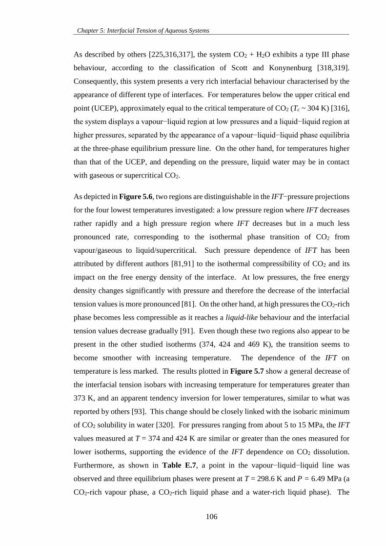
Chapter 5: Interfacial Tension of Aqueous Systems
106
As described by others [225,316,317], the system CO2 + H2O exhibits a type III phase
behaviour, according to the classification of Scott and Konynenburg [318,319].
Consequently, this system presents a very rich interfacial behaviour characterised by the
appearance of different type of interfaces. For temperatures below the upper critical end
point (UCEP), approximately equal to the critical temperature of CO2 (Tc ~ 304 K) [316],
the system displays a vapour−liquid region at low pressures and a liquid−liquid region at
higher pressures, separated by the appearance of a vapour−liquid−liquid phase equilibria
at the three-phase equilibrium pressure line. On the other hand, for temperatures higher
than that of the UCEP, and depending on the pressure, liquid water may be in contact
with gaseous or supercritical CO2.
As depicted in Figure 5.6, two regions are distinguishable in the IFT−pressure projections
for the four lowest temperatures investigated: a low pressure region where IFT decreases
rather rapidly and a high pressure region where IFT decreases but in a much less
pronounced rate, corresponding to the isothermal phase transition of CO2 from
vapour/gaseous to liquid/supercritical. Such pressure dependence of IFT has been
attributed by different authors [81,91] to the isothermal compressibility of CO2 and its
impact on the free energy density of the interface. At low pressures, the free energy
density changes significantly with pressure and therefore the decrease of the interfacial
tension values is more pronounced [81]. On the other hand, at high pressures the CO2-rich
phase becomes less compressible as it reaches a liquid-like behaviour and the interfacial
tension values decrease gradually [91]. Even though these two regions also appear to be
present in the other studied isotherms (374, 424 and 469 K), the transition seems to
become smoother with increasing temperature. The dependence of the IFT on
temperature is less marked. The results plotted in Figure 5.7 show a general decrease of
the interfacial tension isobars with increasing temperature for temperatures greater than
373 K, and an apparent tendency inversion for lower temperatures, similar to what was
reported by others [93]. This change should be closely linked with the isobaric minimum
of CO2 solubility in water [320]. For pressures ranging from about 5 to 15 MPa, the IFT
values measured at T = 374 and 424 K are similar or greater than the ones measured for
lower isotherms, supporting the evidence of the IFT dependence on CO2 dissolution.
Furthermore, as shown in Table E.7, a point in the vapour−liquid−liquid line was
observed and three equilibrium phases were present at T = 298.6 K and P = 6.49 MPa (a
CO2-rich vapour phase, a CO2-rich liquid phase and a water-rich liquid phase). The
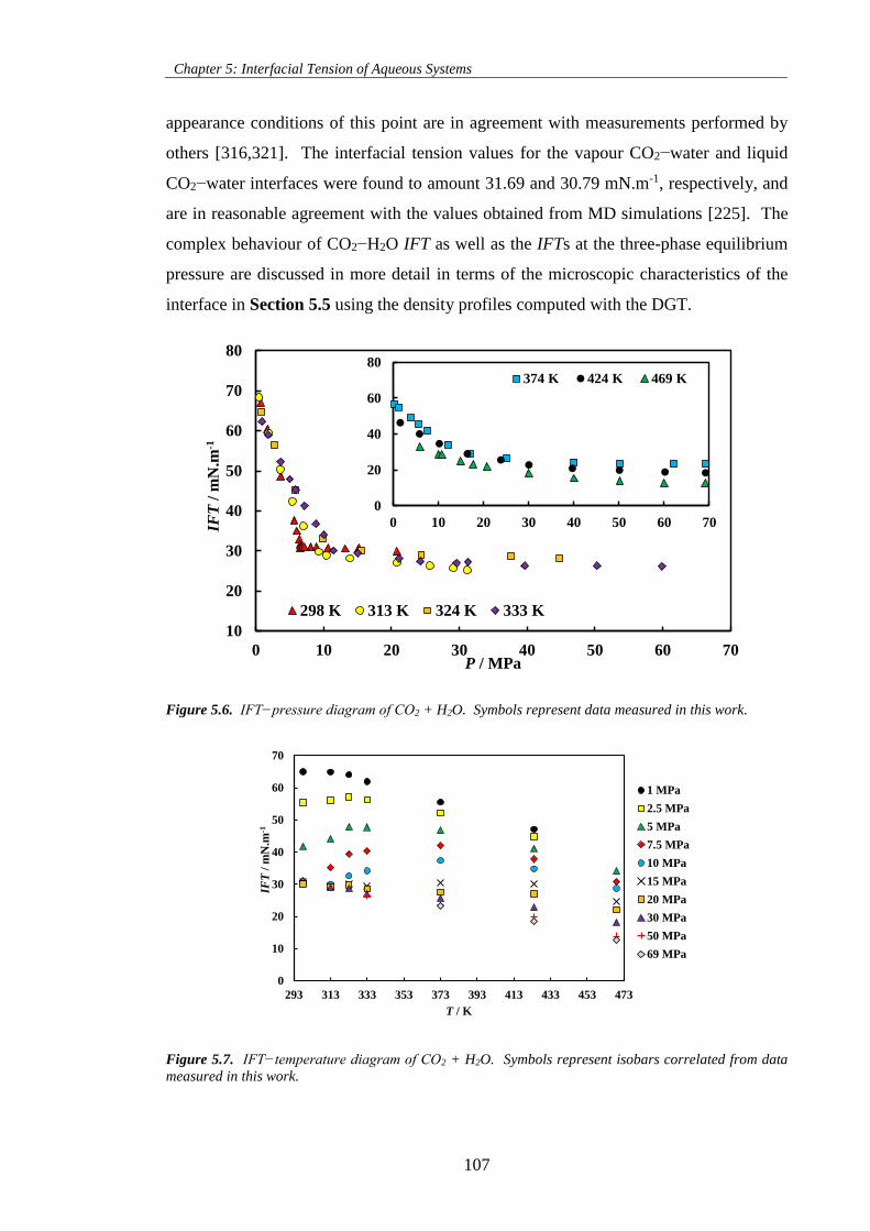
Chapter 5: Interfacial Tension of Aqueous Systems
107
appearance conditions of this point are in agreement with measurements performed by
others [316,321]. The interfacial tension values for the vapour CO2−water and liquid
CO2−water interfaces were found to amount 31.69 and 30.79 mN.m-1, respectively, and
are in reasonable agreement with the values obtained from MD simulations [225]. The
complex behaviour of CO2−H2O IFT as well as the IFTs at the three-phase equilibrium
pressure are discussed in more detail in terms of the microscopic characteristics of the
interface in Section 5.5 using the density profiles computed with the DGT.
Figure 5.6. IFT−pressure diagram of CO2 + H2O. Symbols represent data measured in this work.
Figure 5.7. IFT−temperature diagram of CO2 + H2O. Symbols represent isobars correlated from data
measured in this work.
10
20
30
40
50
60
70
80
0 10 20 30 40 50 60 70
IFT
/ m
N.m
-1
P / MPa
298 K 313 K 324 K 333 K
0
20
40
60
80
0 10 20 30 40 50 60 70
374 K 424 K 469 K
0
10
20
30
40
50
60
70
293 313 333 353 373 393 413 433 453 473
IFT
/ m
N.m
-1
T / K
1 MPa
2.5 MPa
5 MPa
7.5 MPa
10 MPa
15 MPa
20 MPa
30 MPa
50 MPa
69 MPa
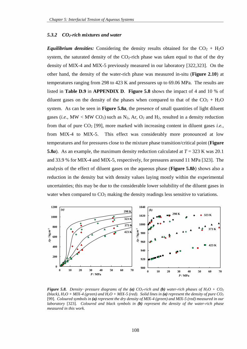
Chapter 5: Interfacial Tension of Aqueous Systems
108
5.3.2 CO2-rich mixtures and water
Equilibrium densities: Considering the density results obtained for the CO2 + H2O
system, the saturated density of the CO2-rich phase was taken equal to that of the dry
density of MIX-4 and MIX-5 previously measured in our laboratory [322,323]. On the
other hand, the density of the water-rich phase was measured in-situ (Figure 2.10) at
temperatures ranging from 298 to 423 K and pressures up to 69.06 MPa. The results are
listed in Table D.9 in APPENDIX D. Figure 5.8 shows the impact of 4 and 10 % of
diluent gases on the density of the phases when compared to that of the CO2 + H2O
system. As can be seen in Figure 5.8a, the presence of small quantities of light diluent
gases (i.e., MW < MW CO2) such as N2, Ar, O2 and H2, resulted in a density reduction
from that of pure CO2 [99], more marked with increasing content in diluent gases i.e.,
from MIX-4 to MIX-5. This effect was considerably more pronounced at low
temperatures and for pressures close to the mixture phase transition/critical point (Figure
5.8a). As an example, the maximum density reduction calculated at T = 323 K was 20.1
and 33.9 % for MIX-4 and MIX-5, respectively, for pressures around 11 MPa [323]. The
analysis of the effect of diluent gases on the aqueous phase (Figure 5.8b) shows also a
reduction in the density but with density values laying mostly within the experimental
uncertainties; this may be due to the considerable lower solubility of the diluent gases in
water when compared to CO2 making the density readings less sensitive to variations.
Figure 5.8. Density−pressure diagrams of the (a) CO2-rich and (b) water-rich phases of H2O + CO2
(black), H2O + MIX-4 (green) and H2O + MIX-5 (red). Solid lines in (a) represent the density of pure CO2
[99]. Coloured symbols in (a) represent the dry density of MIX-4 (green) and MIX-5 (red) measured in our
laboratory [323]. Coloured and black symbols in (b) represent the density of the water-rich phase
measured in this work.
900
920
940
960
980
1000
1020
1040
0 10 20 30 40 50 60 70
Δρ
/ k
g.m
-3
P / MPa
423 K
373 K
323 K298 K
0
200
400
600
800
1000
1200
0 10 20 30 40 50 60 70
Δρ
/ k
g.m
-3
P / MPa
423 K
373 K
323 K
298 K(a) (b)
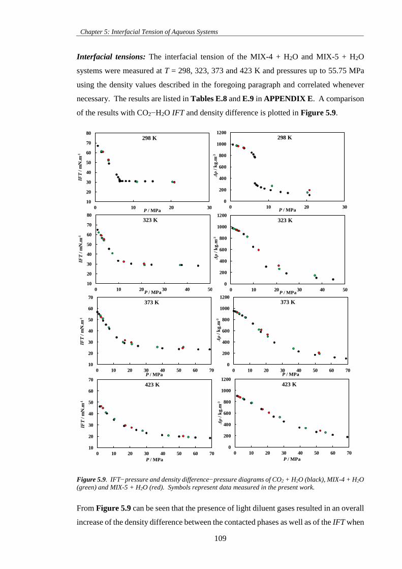
Chapter 5: Interfacial Tension of Aqueous Systems
109
Interfacial tensions: The interfacial tension of the MIX-4 + H2O and MIX-5 + H2O
systems were measured at T = 298, 323, 373 and 423 K and pressures up to 55.75 MPa
using the density values described in the foregoing paragraph and correlated whenever
necessary. The results are listed in Tables E.8 and E.9 in APPENDIX E. A comparison
of the results with CO2−H2O IFT and density difference is plotted in Figure 5.9.
Figure 5.9. IFT−pressure and density difference−pressure diagrams of CO2 + H2O (black), MIX-4 + H2O
(green) and MIX-5 + H2O (red). Symbols represent data measured in the present work.
From Figure 5.9 can be seen that the presence of light diluent gases resulted in an overall
increase of the density difference between the contacted phases as well as of the IFT when
10
20
30
40
50
60
70
80
0 10 20 30
IFT
/ m
N.m
-1
P / MPa
298 K
10
20
30
40
50
60
70
80
0 10 20 30 40 50
IFT
/ m
N.m
-1
P / MPa
323 K
10
20
30
40
50
60
70
0 10 20 30 40 50 60 70
IFT
/ m
N.m
-1
P / MPa
373 K
10
20
30
40
50
60
70
0 10 20 30 40 50 60 70
IFT
/ m
N.m
-1
P / MPa
423 K
0
200
400
600
800
1000
1200
0 10 20 30
Δρ
/ k
g.m
-3P / MPa
298 K
0
200
400
600
800
1000
1200
0 10 20 30 40 50
Δρ
/ k
g.m
-3
P / MPa
323 K
0
200
400
600
800
1000
1200
0 10 20 30 40 50 60 70
Δρ
/ k
g.m
-3
P / MPa
373 K
0
200
400
600
800
1000
1200
0 10 20 30 40 50 60 70
Δρ
/ k
g.m
-3
P / MPa
423 K
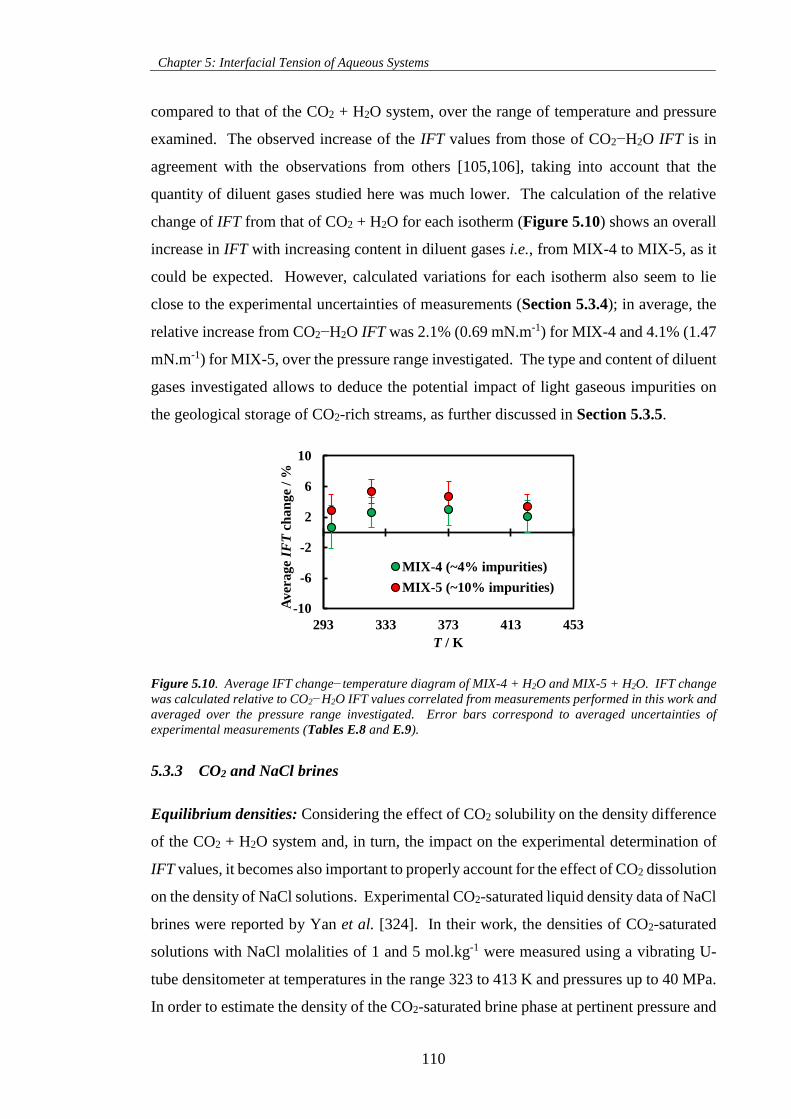
Chapter 5: Interfacial Tension of Aqueous Systems
110
compared to that of the CO2 + H2O system, over the range of temperature and pressure
examined. The observed increase of the IFT values from those of CO2−H2O IFT is in
agreement with the observations from others [105,106], taking into account that the
quantity of diluent gases studied here was much lower. The calculation of the relative
change of IFT from that of CO2 + H2O for each isotherm (Figure 5.10) shows an overall
increase in IFT with increasing content in diluent gases i.e., from MIX-4 to MIX-5, as it
could be expected. However, calculated variations for each isotherm also seem to lie
close to the experimental uncertainties of measurements (Section 5.3.4); in average, the
relative increase from CO2−H2O IFT was 2.1% (0.69 mN.m-1) for MIX-4 and 4.1% (1.47
mN.m-1) for MIX-5, over the pressure range investigated. The type and content of diluent
gases investigated allows to deduce the potential impact of light gaseous impurities on
the geological storage of CO2-rich streams, as further discussed in Section 5.3.5.
Figure 5.10. Average IFT change−temperature diagram of MIX-4 + H2O and MIX-5 + H2O. IFT change
was calculated relative to CO2−H2O IFT values correlated from measurements performed in this work and
averaged over the pressure range investigated. Error bars correspond to averaged uncertainties of
experimental measurements (Tables E.8 and E.9).
5.3.3 CO2 and NaCl brines
Equilibrium densities: Considering the effect of CO2 solubility on the density difference
of the CO2 + H2O system and, in turn, the impact on the experimental determination of
IFT values, it becomes also important to properly account for the effect of CO2 dissolution
on the density of NaCl solutions. Experimental CO2-saturated liquid density data of NaCl
brines were reported by Yan et al. [324]. In their work, the densities of CO2-saturated
solutions with NaCl molalities of 1 and 5 mol.kg-1 were measured using a vibrating U-
tube densitometer at temperatures in the range 323 to 413 K and pressures up to 40 MPa.
In order to estimate the density of the CO2-saturated brine phase at pertinent pressure and
-10
-6
-2
2
6
10
293 333 373 413 453
Av
era
ge
IFT
cha
ng
e /
%
T / K
MIX-4 (~4% impurities)
MIX-5 (~10% impurities)
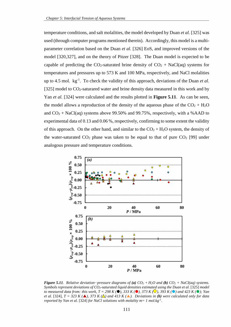
Chapter 5: Interfacial Tension of Aqueous Systems
111
temperature conditions, and salt molalities, the model developed by Duan et al. [325] was
used (through computer programs mentioned therein). Accordingly, this model is a multi-
parameter correlation based on the Duan et al. [326] EoS, and improved versions of the
model [320,327], and on the theory of Pitzer [328]. The Duan model is expected to be
capable of predicting the CO2-saturated brine density of CO2 + NaCl(aq) systems for
temperatures and pressures up to 573 K and 100 MPa, respectively, and NaCl molalities
up to 4.5 mol. kg-1. To check the validity of this approach, deviations of the Duan et al.
[325] model to CO2-saturared water and brine density data measured in this work and by
Yan et al. [324] were calculated and the results plotted in Figure 5.11. As can be seen,
the model allows a reproduction of the density of the aqueous phase of the CO2 + H2O
and CO2 + NaCl(aq) systems above 99.50% and 99.75%, respectively, with a %AAD to
experimental data of 0.13 and 0.06 %, respectively, confirming to some extent the validity
of this approach. On the other hand, and similar to the CO2 + H2O system, the density of
the water-saturated CO2 phase was taken to be equal to that of pure CO2 [99] under
analogous pressure and temperature conditions.
Figure 5.11. Relative deviation−pressure diagrams of (a) CO2 + H2O and (b) CO2 + NaCl(aq) systems.
Symbols represent deviations of CO2-saturated liquid densities estimated using the Duan et al. [325] model
to measured data from: this work, T = 298 K (), 333 K (), 373 K ( ), 393 K () and 423 K (); Yan
et al. [324], T = 323 K (), 373 K ( ) and 413 K (). Deviations in (b) were calculated only for data
reported by Yan et al. [324] for NaCl solutions with molality m= 1 mol.kg-1.
-0.75
-0.50
-0.25
0.00
0.25
0.50
0.75
0 20 40 60 80
(ρex
p–
ρest)/
ρex
p×
10
0 %
P / MPa
-0.75
-0.50
-0.25
0.00
0.25
0.50
0.75
0 20 40 60 80
(ρex
p–
ρest)/
ρex
p×
10
0 %
P / MPa
(a)
(b)
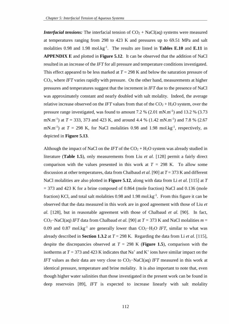
Chapter 5: Interfacial Tension of Aqueous Systems
112
Interfacial tensions: The interfacial tension of CO2 + NaCl(aq) systems were measured
at temperatures ranging from 298 to 423 K and pressures up to 69.51 MPa and salt
molalities 0.98 and 1.98 mol.kg-1. The results are listed in Tables E.10 and E.11 in
APPENDIX E and plotted in Figure 5.12. It can be observed that the addition of NaCl
resulted in an increase of the IFT for all pressure and temperature conditions investigated.
This effect appeared to be less marked at T = 298 K and below the saturation pressure of
CO2, where IFT varies rapidly with pressure. On the other hand, measurements at higher
pressures and temperatures suggest that the increment in IFT due to the presence of NaCl
was approximately constant and nearly doubled with salt molality. Indeed, the average
relative increase observed on the IFT values from that of the CO2 + H2O system, over the
pressure range investigated, was found to amount 7.2 % (2.01 mN.m-1) and 13.2 % (3.73
mN.m-1) at T = 333, 373 and 423 K, and around 4.4 % (1.42 mN.m-1) and 7.8 % (2.67
mN.m-1) at T = 298 K, for NaCl molalities 0.98 and 1.98 mol.kg-1, respectively, as
depicted in Figure 5.13.
Although the impact of NaCl on the IFT of the CO2 + H2O system was already studied in
literature (Table 1.5), only measurements from Liu et al. [128] permit a fairly direct
comparison with the values presented in this work at T = 298 K. To allow some
discussion at other temperatures, data from Chalbaud et al. [90] at T = 373 K and different
NaCl molalities are also plotted in Figure 5.12, along with data from Li et al. [115] at T
= 373 and 423 K for a brine composed of 0.864 (mole fraction) NaCl and 0.136 (mole
fraction) KCl, and total salt molalities 0.98 and 1.98 mol.kg-1. From this figure it can be
observed that the data measured in this work are in good agreement with those of Liu et
al. [128], but in reasonable agreement with those of Chalbaud et al. [90]. In fact,
CO2−NaCl(aq) IFT data from Chalbaud et al. [90] at T = 373 K and NaCl molalities m =
0.09 and 0.87 mol.kg-1 are generally lower than CO2−H2O IFT, similar to what was
already described in Section 1.3.2 at T = 298 K. Regarding the data from Li et al. [115],
despite the discrepancies observed at T = 298 K (Figure 1.5), comparison with the
isotherms at T = 373 and 423 K indicates that Na+ and K+ ions have similar impact on the
IFT values as their data are very close to CO2−NaCl(aq) IFT measured in this work at
identical pressure, temperature and brine molality. It is also important to note that, even
though higher water salinities than those investigated in the present work can be found in
deep reservoirs [89], IFT is expected to increase linearly with salt molality
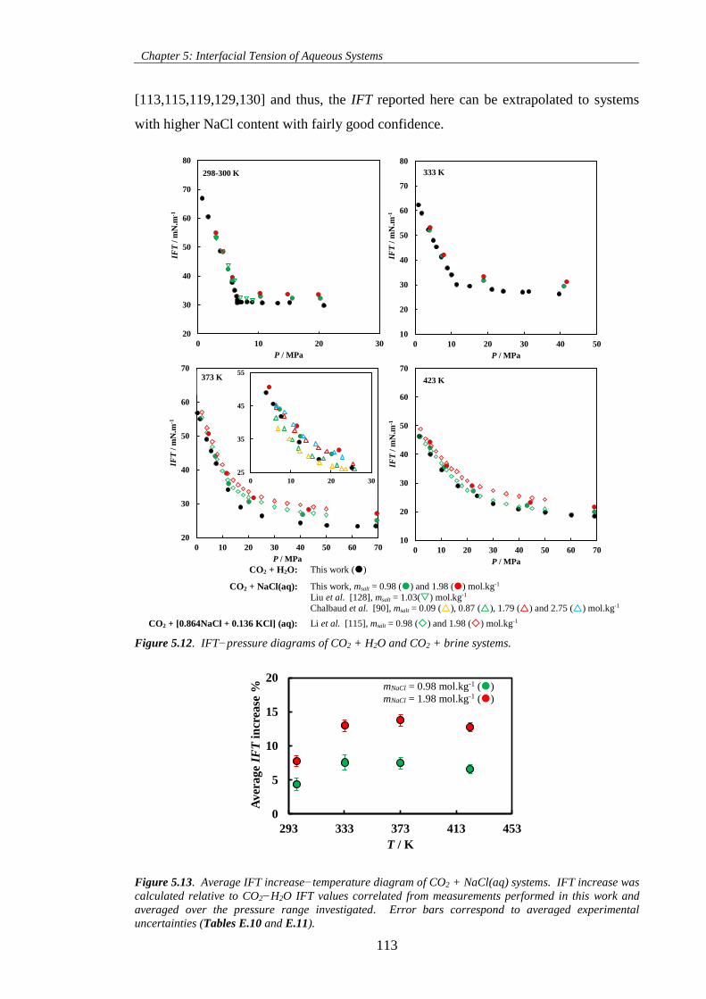
Chapter 5: Interfacial Tension of Aqueous Systems
113
[113,115,119,129,130] and thus, the IFT reported here can be extrapolated to systems
with higher NaCl content with fairly good confidence.
Figure 5.12. IFT−pressure diagrams of CO2 + H2O and CO2 + brine systems.
Figure 5.13. Average IFT increase−temperature diagram of CO2 + NaCl(aq) systems. IFT increase was
calculated relative to CO2−H2O IFT values correlated from measurements performed in this work and
averaged over the pressure range investigated. Error bars correspond to averaged experimental
uncertainties (Tables E.10 and E.11).
20
30
40
50
60
70
80
0 10 20 30
IFT
/ m
N.m
-1
P / MPa
10
20
30
40
50
60
70
80
0 10 20 30 40 50
IFT
/ m
N.m
-1
P / MPa
20
30
40
50
60
70
0 10 20 30 40 50 60 70
IFT
/ m
N.m
-1
P / MPa
10
20
30
40
50
60
70
0 10 20 30 40 50 60 70
IFT
/ m
N.m
-1
P / MPa
298-300 K
373 K
333 K
423 K
25
35
45
55
0 10 20 30
0
5
10
15
20
293 333 373 413 453
Av
era
ge
IFT
incr
ease
%
T / K
CO2 + H2O: This work ()
CO2 + NaCl(aq): This work, msalt = 0.98 () and 1.98 () mol.kg-1
Liu et al. [128], msalt = 1.03() mol.kg-1 Chalbaud et al. [90], msalt = 0.09 (), 0.87 (), 1.79 () and 2.75 () mol.kg-1
CO2 + [0.864NaCl + 0.136 KCl] (aq): Li et al. [115], msalt = 0.98 () and 1.98 () mol.kg-1
mNaCl = 0.98 mol.kg-1 ()
mNaCl = 1.98 mol.kg-1 ()
Chapter 5: Interfacial Tension of Aqueous Systems
114
5.3.4 Experimental uncertainties
The combined expanded uncertainties in the interfacial tension measurements, Uc (IFT),
are assessed by combining the uncertainties on the drop shape analysis for each recorded
image, U1 (IFT), and uncertainties on the estimation of the density difference for the
equilibrated phases, U2 (IFT). The first contribution can be estimated, to some extent, by
the standard deviation of the interfacial tension values calculated from the recorded
images at each experimental condition. This statistical standard error includes the errors
and uncertainties from the use of the Laplace equation, vibrations and reproducibility of
the measurements. The effect of uncertainties in pressure and temperature in determining
the density of the saturated phases used in the interfacial tension calculations can be
evaluated by the law of propagation of errors as follows [296]:
2 2
2 2
1/22 2
2 2
2 ( ) ( ) ( )c H O c CO
H O CO
IFT IFTU IFT U U
5.3
1/22 2
2 2( ) ( ) ( )cU u P u TP T
5.4
The combined expanded uncertainties in the IFT measurements, estimated with a
confidence level of 0.95, are shown in Tables E.7 through E.11 for each system and
experimental condition. It can be observed that in general, the uncertainties caused by
the density of the phases are greater than the uncertainties that arise from the ASDA
method. Overall, the combined expanded uncertainty averaged 0.31 mN.m-1 for the CO2
+ H2O system, 0.67 mN.m-1 for the MIX-4 + H2O and MIX-5 + H2O systems, and 0.27
mN.m-1 for the CO2 + NaCl(aq) systems. A maximum uncertainty of 1.87 mN.m-1 was
estimated at the three-phase equilibrium point of the CO2 + H2O system for the IFT value
between the CO2-rich liquid and the water-rich liquid phases.
5.3.5 Implications on the geological storage of CO2
Considering the wide range of experimental conditions investigated in the foregoing
sections, it is now possible to study the impact of interfacial tension on the geological
storage of CO2. This analysis was performed by deducing the impact of temperature and
pressure, as well as of fluids properties, on the column of CO2 that can be trapped beneath
a caprock due to variations on CO2−H2O IFT via Equation 1.8 (structural trapping). For
Chapter 5: Interfacial Tension of Aqueous Systems
115
the sake of simplicity and as a first approximation, some considerations, based on the
works of others [7,33], have been made:
Type of reservoir: aquifer;
Reservoir fluids: carbon dioxide and water;
The caprock is considered to be fully water wet (cos θ = 1) and with pores of
cylindrical shape and average radius R = 0.1 μm;
The values of porosity and residual water saturation of the reservoir are assumed
to be ϕ = 0.3 and Sw =0.1;
The aforementioned properties of the caprock and reservoir are assumed to be
evenly distributed and constant with depth;
Pores above the caprock are considered to be filled with water, thus the pressure
felt in the caprock is deduced using a hydrostatic gradient of 10 MPa.km-1;
Temperature felt in the caprock is deduced using two geothermal gradients: 30
and 40 K.km-1;
The density of CO2, calculated with REFPROP [99] at the caprock’s temperature
and pressure, is considered to be constant throughout the reservoir (i.e., along H).
The density of water is calculated using Equation 5.1. The dissolution of CO2 in
the aquifer below the reservoir is not considered;
The maximum amount of CO2 that can be trapped beneath the caprock is estimated
using CO2−H2O IFT values correlated from the isotherms investigated in this
work.
Under these assumptions, the column of CO2 that the caprock can safely sustain and, in
turn, the CO2 storage capacity (in millions of tons per km2 i.e., Mt.km-2) of an underlying
reservoir are estimated via Equation 1.9 as function of caprock depth. Estimations were
performed considering two different field scenarios: onshore, with a surface temperature
and pressure of 288 K and 0.1 MPa, respectively, and offshore, with a seabed temperature
and pressure of 277 K and 10 MPa, respectively. Figure 5.14 shows schematically some
of the foregoing assumptions. The results are plotted in Figures 5.15 and 5.16 along with
the variation of CO2−H2O IFT and CO2 density with caprock depth.
The results plotted in Figure 5.15a suggest that CO2 storage capacity in an onshore field
increases with caprock depths up to 2 km and levels off for depths up to 4 km. This
behaviour is in good agreement with that described by Chiquet et al. [7] for a caprock and
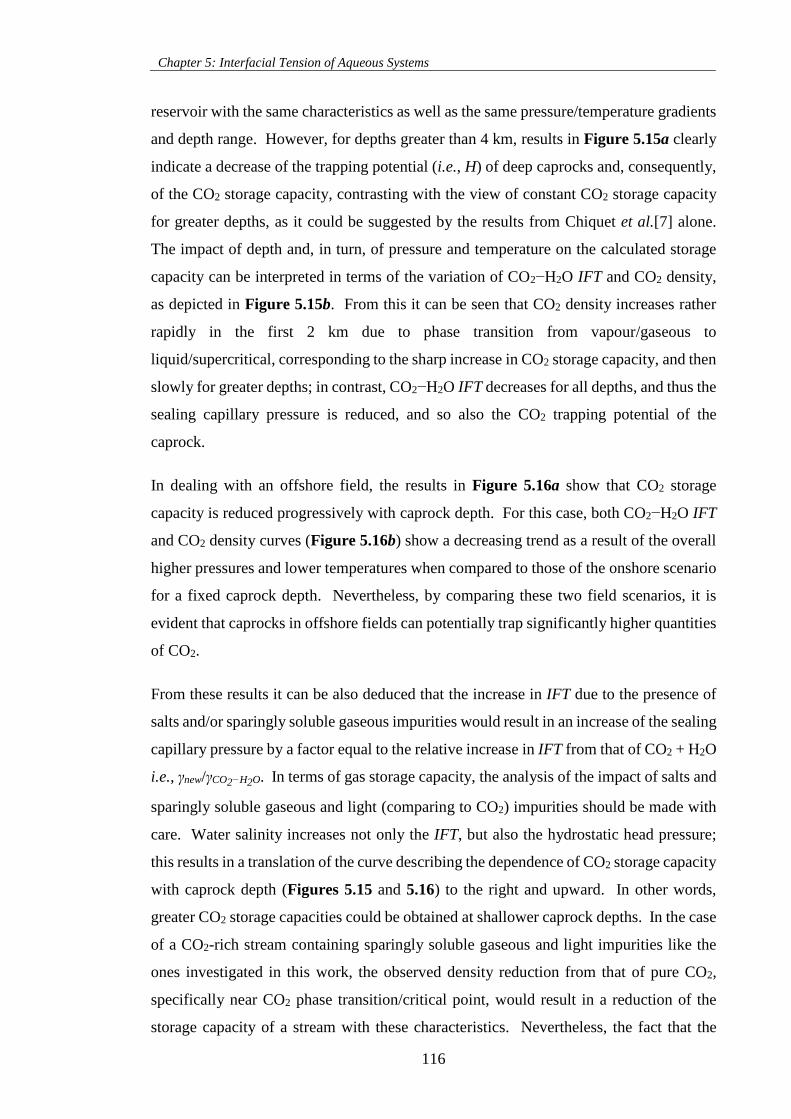
Chapter 5: Interfacial Tension of Aqueous Systems
116
reservoir with the same characteristics as well as the same pressure/temperature gradients
and depth range. However, for depths greater than 4 km, results in Figure 5.15a clearly
indicate a decrease of the trapping potential (i.e., H) of deep caprocks and, consequently,
of the CO2 storage capacity, contrasting with the view of constant CO2 storage capacity
for greater depths, as it could be suggested by the results from Chiquet et al.[7] alone.
The impact of depth and, in turn, of pressure and temperature on the calculated storage
capacity can be interpreted in terms of the variation of CO2−H2O IFT and CO2 density,
as depicted in Figure 5.15b. From this it can be seen that CO2 density increases rather
rapidly in the first 2 km due to phase transition from vapour/gaseous to
liquid/supercritical, corresponding to the sharp increase in CO2 storage capacity, and then
slowly for greater depths; in contrast, CO2−H2O IFT decreases for all depths, and thus the
sealing capillary pressure is reduced, and so also the CO2 trapping potential of the
caprock.
In dealing with an offshore field, the results in Figure 5.16a show that CO2 storage
capacity is reduced progressively with caprock depth. For this case, both CO2−H2O IFT
and CO2 density curves (Figure 5.16b) show a decreasing trend as a result of the overall
higher pressures and lower temperatures when compared to those of the onshore scenario
for a fixed caprock depth. Nevertheless, by comparing these two field scenarios, it is
evident that caprocks in offshore fields can potentially trap significantly higher quantities
of CO2.
From these results it can be also deduced that the increase in IFT due to the presence of
salts and/or sparingly soluble gaseous impurities would result in an increase of the sealing
capillary pressure by a factor equal to the relative increase in IFT from that of CO2 + H2O
i.e., γnew/γCO2−H2O. In terms of gas storage capacity, the analysis of the impact of salts and
sparingly soluble gaseous and light (comparing to CO2) impurities should be made with
care. Water salinity increases not only the IFT, but also the hydrostatic head pressure;
this results in a translation of the curve describing the dependence of CO2 storage capacity
with caprock depth (Figures 5.15 and 5.16) to the right and upward. In other words,
greater CO2 storage capacities could be obtained at shallower caprock depths. In the case
of a CO2-rich stream containing sparingly soluble gaseous and light impurities like the
ones investigated in this work, the observed density reduction from that of pure CO2,
specifically near CO2 phase transition/critical point, would result in a reduction of the
storage capacity of a stream with these characteristics. Nevertheless, the fact that the
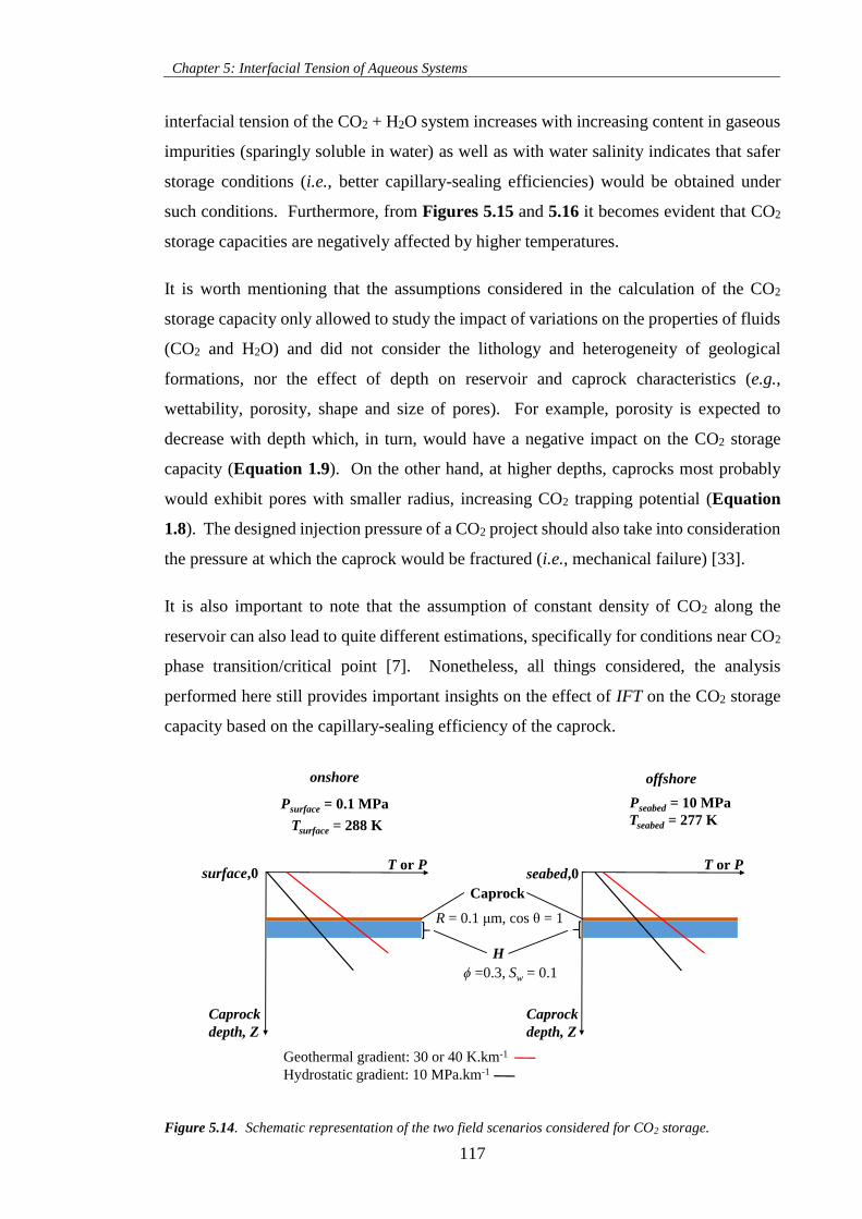
Chapter 5: Interfacial Tension of Aqueous Systems
117
interfacial tension of the CO2 + H2O system increases with increasing content in gaseous
impurities (sparingly soluble in water) as well as with water salinity indicates that safer
storage conditions (i.e., better capillary-sealing efficiencies) would be obtained under
such conditions. Furthermore, from Figures 5.15 and 5.16 it becomes evident that CO2
storage capacities are negatively affected by higher temperatures.
It is worth mentioning that the assumptions considered in the calculation of the CO2
storage capacity only allowed to study the impact of variations on the properties of fluids
(CO2 and H2O) and did not consider the lithology and heterogeneity of geological
formations, nor the effect of depth on reservoir and caprock characteristics (e.g.,
wettability, porosity, shape and size of pores). For example, porosity is expected to
decrease with depth which, in turn, would have a negative impact on the CO2 storage
capacity (Equation 1.9). On the other hand, at higher depths, caprocks most probably
would exhibit pores with smaller radius, increasing CO2 trapping potential (Equation
1.8). The designed injection pressure of a CO2 project should also take into consideration
the pressure at which the caprock would be fractured (i.e., mechanical failure) [33].
It is also important to note that the assumption of constant density of CO2 along the
reservoir can also lead to quite different estimations, specifically for conditions near CO2
phase transition/critical point [7]. Nonetheless, all things considered, the analysis
performed here still provides important insights on the effect of IFT on the CO2 storage
capacity based on the capillary-sealing efficiency of the caprock.
Figure 5.14. Schematic representation of the two field scenarios considered for CO2 storage.
onshore
Caprock
depth, Z
T or Psurface,0
H
Caprock
Caprock
depth, Z
T or P
offshore
Psurface = 0.1 MPa
Tsurface = 288 K
seabed,0
Pseabed = 10 MPa
Tseabed = 277 K
Geothermal gradient: 30 or 40 K.km-1
Hydrostatic gradient: 10 MPa.km-1
ϕ =0.3, Sw = 0.1
R = 0.1 μm, cos θ = 1
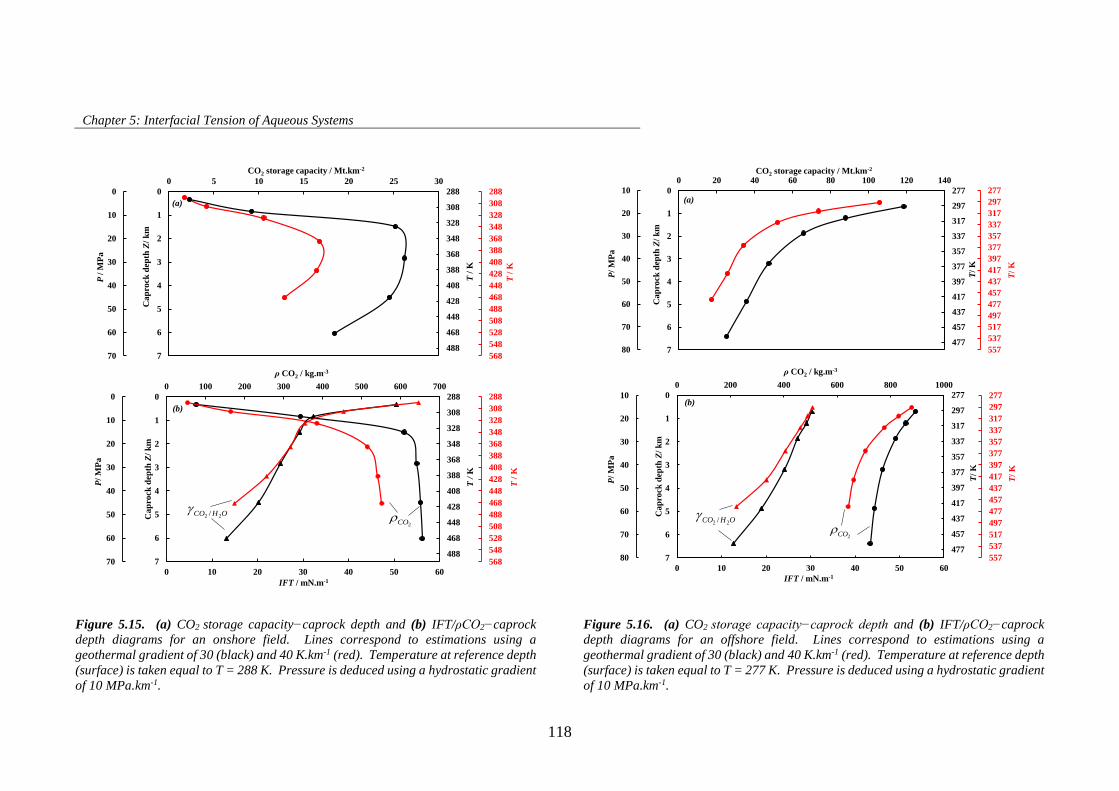
Chapter 5: Interfacial Tension of Aqueous Systems
118
Figure 5.15. (a) CO2 storage capacity−caprock depth and (b) IFT/ρCO2−caprock
depth diagrams for an onshore field. Lines correspond to estimations using a
geothermal gradient of 30 (black) and 40 K.km-1 (red). Temperature at reference depth
(surface) is taken equal to T = 288 K. Pressure is deduced using a hydrostatic gradient
of 10 MPa.km-1.
Figure 5.16. (a) CO2 storage capacity−caprock depth and (b) IFT/ρCO2−caprock
depth diagrams for an offshore field. Lines correspond to estimations using a
geothermal gradient of 30 (black) and 40 K.km-1 (red). Temperature at reference depth
(surface) is taken equal to T = 277 K. Pressure is deduced using a hydrostatic gradient
of 10 MPa.km-1.
0 10 20 30 40 50 60
0
1
2
3
4
5
6
7
0 100 200 300 400 500 600 700
IFT / (mN.m-1)
Ca
pro
ck d
epth
Z/
km
ρ CO2/ (kg.m-3)
288
308
328
348
368
388
408
428
448
468
488
508
528
548
568
0
10
20
30
40
50
60
70
T /
K
P/
MP
a
288
308
328
348
368
388
408
428
448
468
488
T /
K
288
308
328
348
368
388
408
428
448
468
488
0
1
2
3
4
5
6
7
0 5 10 15 20 25 30
T /
K
Ca
pro
ck d
epth
Z/
km
CO2 storage capacity/ (Mt.km-2)
288
308
328
348
368
388
408
428
448
468
488
508
528
548
568
0
10
20
30
40
50
60
70
T /
K
P /
MP
a
2 2/CO H O2CO
(a)
(b)
T /
K
CO2 storage capacity / Mt.km-2
ρ CO2 / kg.m-3
IFT / mN.m-1
277
297
317
337
357
377
397
417
437
457
477
0
1
2
3
4
5
6
7
0 20 40 60 80 100 120 140
T /
K
Ca
pro
ck d
epth
Z/
km
CO2 storage capacity/ (Mt.km-2)
277
297
317
337
357
377
397
417
437
457
477
497
517
537
557
10
20
30
40
50
60
70
80
T/
K
P/
MP
a
277
297
317
337
357
377
397
417
437
457
477
497
517
537
557
10
20
30
40
50
60
70
80
T/
K
P/
MP
a
0
1
2
3
4
5
6
7
0 10 20 30 40 50 60
0
1
2
3
4
5
6
7
0 200 400 600 800 1000
IFT / (mN.m-1)
Ca
pro
ck d
epth
Z/
km
ρ CO2/ (kg.m-3)
277
297
317
337
357
377
397
417
437
457
477
T/
K
2 2/CO H O
2CO
(a)
(b)
T/
K
CO2 storage capacity / Mt.km-2
ρ CO2 / kg.m-3
IFT / mN.m-1
Chapter 5: Interfacial Tension of Aqueous Systems
119
5.4 Modelling
5.4.1 Binary mixtures
In this section the DGT was coupled with the CPA EoS and its ability to describe both
bulk phase and interfacial properties of binary aqueous systems was evaluated by
comparison with experimental data from the present work and gathered from literature.
Modelling results were also compared to IFTs computed using Sutton’s correlation and
the LGT. The systems investigated included two-phase interfacial tensions of common
gases (CO2, N2 and CH4) and n-alkanes (n-C6, n-C10 and n-C16) against water over a broad
range of pressure and temperature conditions. For the thermodynamic conditions
examined, the type of interfaces analysed comprised a liquid water phase in contact with
gases in subcritical and/or supercritical conditions, as well as with liquid hydrocarbons.
In order to provide a correct description of the composition of the phases, binary
interaction coefficients within the CPA EoS framework (kijs) were used. The kij values
were taken from previous works, except for N2 + H2O and n-C16 + H2O systems, which
were regressed against solubility data for the aqueous phase and used to predict the
behaviour of the gas/n-alkane-rich phase. Correlated aqueous phase data of N2 + H2O for
pressures up to 60 MPa from the work of Mao and Duan [329] and experimental n-C16
solubility data in the aqueous phase at P = 5 MPa reported in Bergin’s thesis [330] were
used as regression data. In the case of the gas + water systems, the dependence of kij
values on temperature was preserved, whereas for each n-alkane + water system, a single
kij value, temperature independent, was used. All non-aqueous components were
modelled as inert molecules and only cross-association (solvation) between CO2 and H2O
was explicitly incorporated in the model (Section 3.6 and APPENDIX B). The kijs values
used in this work are summarized in Table 5.5 along with the temperature range of
experimental/calculated solubility data used in their regression.
Figures 5.17a through 5.19a show that the CPA EoS is capable of providing a good
description of both gas solubility and water content of the studied gas + water systems
over a broad range of pressures and temperatures, including near and at CO2 supercritical
conditions. For the n-alkane + water systems, mutual solubility data at high pressures are
scarce, with experimental studies frequently carried at atmospheric conditions or at
three-phase equilibrium pressures [331–333], hence comparison with solubility data at
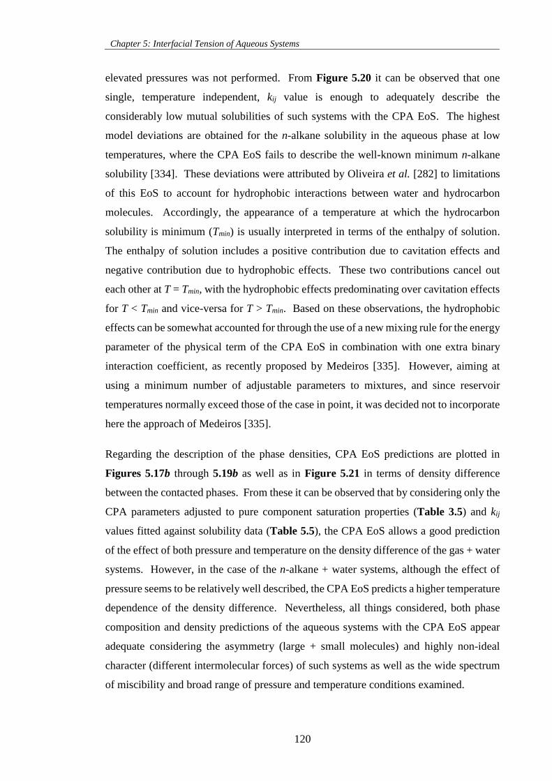
Chapter 5: Interfacial Tension of Aqueous Systems
120
elevated pressures was not performed. From Figure 5.20 it can be observed that one
single, temperature independent, kij value is enough to adequately describe the
considerably low mutual solubilities of such systems with the CPA EoS. The highest
model deviations are obtained for the n-alkane solubility in the aqueous phase at low
temperatures, where the CPA EoS fails to describe the well-known minimum n-alkane
solubility [334]. These deviations were attributed by Oliveira et al. [282] to limitations
of this EoS to account for hydrophobic interactions between water and hydrocarbon
molecules. Accordingly, the appearance of a temperature at which the hydrocarbon
solubility is minimum (Tmin) is usually interpreted in terms of the enthalpy of solution.
The enthalpy of solution includes a positive contribution due to cavitation effects and
negative contribution due to hydrophobic effects. These two contributions cancel out
each other at T = Tmin, with the hydrophobic effects predominating over cavitation effects
for T < Tmin and vice-versa for T > Tmin. Based on these observations, the hydrophobic
effects can be somewhat accounted for through the use of a new mixing rule for the energy
parameter of the physical term of the CPA EoS in combination with one extra binary
interaction coefficient, as recently proposed by Medeiros [335]. However, aiming at
using a minimum number of adjustable parameters to mixtures, and since reservoir
temperatures normally exceed those of the case in point, it was decided not to incorporate
here the approach of Medeiros [335].
Regarding the description of the phase densities, CPA EoS predictions are plotted in
Figures 5.17b through 5.19b as well as in Figure 5.21 in terms of density difference
between the contacted phases. From these it can be observed that by considering only the
CPA parameters adjusted to pure component saturation properties (Table 3.5) and kij
values fitted against solubility data (Table 5.5), the CPA EoS allows a good prediction
of the effect of both pressure and temperature on the density difference of the gas + water
systems. However, in the case of the n-alkane + water systems, although the effect of
pressure seems to be relatively well described, the CPA EoS predicts a higher temperature
dependence of the density difference. Nevertheless, all things considered, both phase
composition and density predictions of the aqueous systems with the CPA EoS appear
adequate considering the asymmetry (large + small molecules) and highly non-ideal
character (different intermolecular forces) of such systems as well as the wide spectrum
of miscibility and broad range of pressure and temperature conditions examined.
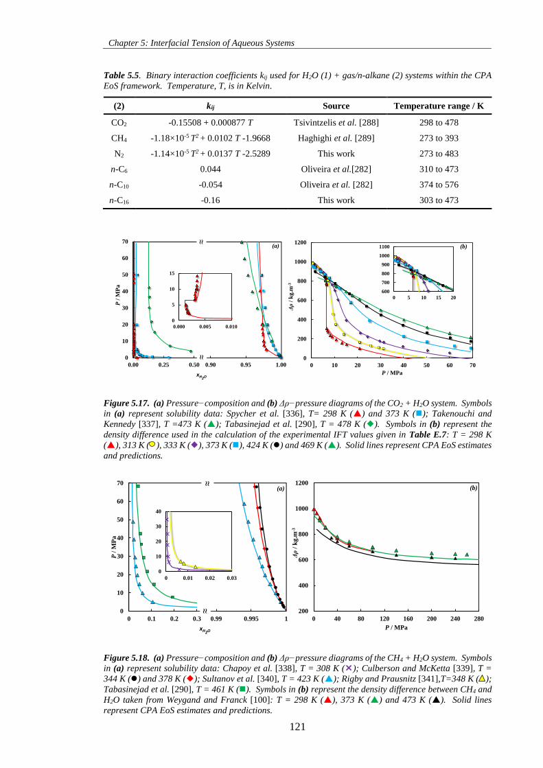
Chapter 5: Interfacial Tension of Aqueous Systems
121
Table 5.5. Binary interaction coefficients kij used for H2O (1) + gas/n-alkane (2) systems within the CPA
EoS framework. Temperature, T, is in Kelvin.
(2) kij Source Temperature range / K
CO2 -0.15508 + 0.000877 T Tsivintzelis et al. [288] 298 to 478
CH4 -1.18×10⁻⁵ T2 + 0.0102 T -1.9668 Haghighi et al. [289] 273 to 393
N2 -1.14×10⁻⁵ T2 + 0.0137 T -2.5289 This work 273 to 483
n-C6 0.044 Oliveira et al.[282] 310 to 473
n-C10 -0.054 Oliveira et al. [282] 374 to 576
n-C16 -0.16 This work 303 to 473
Figure 5.17. (a) Pressure−composition and (b) Δρ−pressure diagrams of the CO2 + H2O system. Symbols
in (a) represent solubility data: Spycher et al. [336], T= 298 K () and 373 K (); Takenouchi and
Kennedy [337], T =473 K (); Tabasinejad et al. [290], T = 478 K (). Symbols in (b) represent the
density difference used in the calculation of the experimental IFT values given in Table E.7: T = 298 K
(), 313 K ( ), 333 K (), 373 K (), 424 K () and 469 K (). Solid lines represent CPA EoS estimates
and predictions.
Figure 5.18. (a) Pressure−composition and (b) Δρ−pressure diagrams of the CH4 + H2O system. Symbols
in (a) represent solubility data: Chapoy et al. [338], T = 308 K (); Culberson and McKetta [339], T =
344 K () and 378 K (); Sultanov et al. [340], T = 423 K (); Rigby and Prausnitz [341],T=348 K ( );
Tabasinejad et al. [290], T = 461 K (). Symbols in (b) represent the density difference between CH4 and
H2O taken from Weygand and Franck [100]: T = 298 K (), 373 K () and 473 K (). Solid lines
represent CPA EoS estimates and predictions.
0.90 0.95 1.00
0
10
20
30
40
50
60
70
0.00 0.25 0.50
P/
MP
a
0
5
10
15
0.000 0.005 0.010
xH2O
≈≈
(a)
0
200
400
600
800
1000
1200
0 10 20 30 40 50 60 70
Δρ
/ k
g.m
-3
P / MPa
(b)
600
700
800
900
1000
1100
0 5 10 15 20
0.99 0.995 1
0
10
20
30
40
50
60
70
0 0.1 0.2 0.3
P/
MP
a
0
10
20
30
40
0 0.01 0.02 0.03
≈≈
xH2O
(a)
200
400
600
800
1000
1200
0 40 80 120 160 200 240 280
Δρ
/ k
g.m
-3
P / MPa
(b)
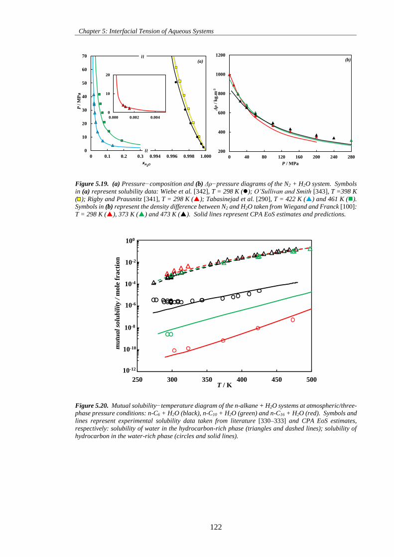
Chapter 5: Interfacial Tension of Aqueous Systems
122
Figure 5.19. (a) Pressure−composition and (b) Δρ−pressure diagrams of the N2 + H2O system. Symbols
in (a) represent solubility data: Wiebe et al. [342], T = 298 K (); O’Sullivan and Smith [343], T =398 K
( ); Rigby and Prausnitz [341], T = 298 K (); Tabasinejad et al. [290], T = 422 K () and 461 K ().
Symbols in (b) represent the density difference between N2 and H2O taken from Wiegand and Franck [100]:
T = 298 K (), 373 K () and 473 K (). Solid lines represent CPA EoS estimates and predictions.
Figure 5.20. Mutual solubility−temperature diagram of the n-alkane + H2O systems at atmospheric/three-
phase pressure conditions: n-C6 + H2O (black), n-C10 + H2O (green) and n-C16 + H2O (red). Symbols and
lines represent experimental solubility data taken from literature [330–333] and CPA EoS estimates,
respectively: solubility of water in the hydrocarbon-rich phase (triangles and dashed lines); solubility of
hydrocarbon in the water-rich phase (circles and solid lines).
0.994 0.996 0.998 1.000
0
10
20
30
40
50
60
70
0 0.1 0.2 0.3
P /
MP
a
≈
xH2O
≈
0
10
20
0.000 0.002 0.004
200
400
600
800
1000
1200
0 40 80 120 160 200 240 280
Δρ
/ k
g.m
-3
P / MPa
(b)(a)
0
0
0
0
0
0
1
250 300 350 400 450 500
mu
tua
l so
lub
ilit
y /
mo
le f
ract
ion
T / K
100
10-2
10-4
10-6
10-8
10-10
10-12
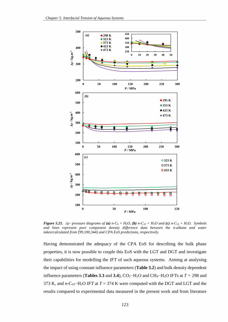
Chapter 5: Interfacial Tension of Aqueous Systems
123
Figure 5.21. Δρ−pressure diagrams of (a) n-C6 + H2O, (b) n-C10 + H2O and (c) n-C16 + H2O. Symbols
and lines represent pure component density difference data between the n-alkane and water
taken/calculated from [99,100,344] and CPA EoS predictions, respectively.
Having demonstrated the adequacy of the CPA EoS for describing the bulk phase
properties, it is now possible to couple this EoS with the LGT and DGT and investigate
their capabilities for modelling the IFT of such aqueous systems. Aiming at analysing
the impact of using constant influence parameters (Table 3.2) and bulk density dependent
influence parameters (Tables 3.3 and 3.4), CO2−H2O and CH4−H2O IFTs at T = 298 and
373 K, and n-C10−H2O IFT at T = 374 K were computed with the DGT and LGT and the
results compared to experimental data measured in the present work and from literature
100
200
300
400
500
600
0 50 100 150
Δρ
/ k
g.m
-3
P / MPa
323 K
373 K
433 K
200
300
400
500
0 50 100 150 200 250 300
Δρ
/ k
g.m
-3
P / MPa
298 K323 K373 K423 K473 K
250
300
350
400
450
0 10 20 30 40 50
100
200
300
400
500
600
0 50 100 150 200 250 300
Δρ
/ k
g.m
-3
P / MPa
295 K
353 K
423 K
473 K
(a)
(b)
(c)
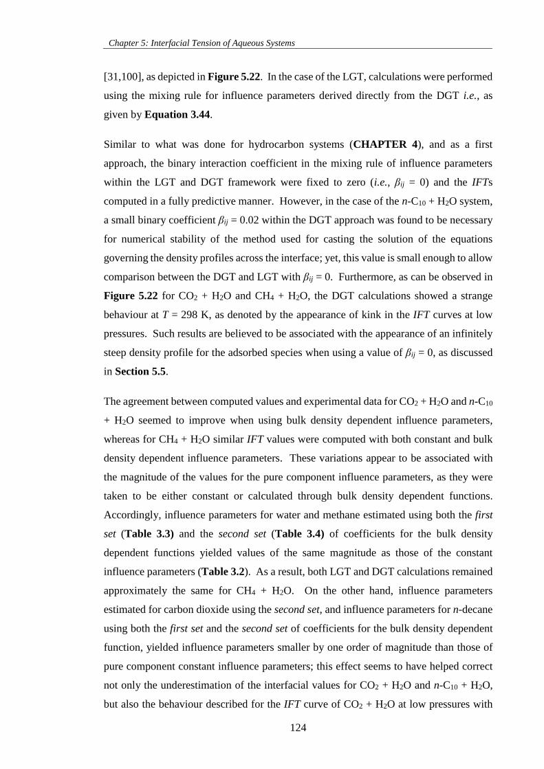
Chapter 5: Interfacial Tension of Aqueous Systems
124
[31,100], as depicted in Figure 5.22. In the case of the LGT, calculations were performed
using the mixing rule for influence parameters derived directly from the DGT i.e., as
given by Equation 3.44.
Similar to what was done for hydrocarbon systems (CHAPTER 4), and as a first
approach, the binary interaction coefficient in the mixing rule of influence parameters
within the LGT and DGT framework were fixed to zero (i.e., βij = 0) and the IFTs
computed in a fully predictive manner. However, in the case of the n-C10 + H2O system,
a small binary coefficient βij = 0.02 within the DGT approach was found to be necessary
for numerical stability of the method used for casting the solution of the equations
governing the density profiles across the interface; yet, this value is small enough to allow
comparison between the DGT and LGT with βij = 0. Furthermore, as can be observed in
Figure 5.22 for CO2 + H2O and CH4 + H2O, the DGT calculations showed a strange
behaviour at T = 298 K, as denoted by the appearance of kink in the IFT curves at low
pressures. Such results are believed to be associated with the appearance of an infinitely
steep density profile for the adsorbed species when using a value of βij = 0, as discussed
in Section 5.5.
The agreement between computed values and experimental data for CO2 + H2O and n-C10
+ H2O seemed to improve when using bulk density dependent influence parameters,
whereas for CH4 + H2O similar IFT values were computed with both constant and bulk
density dependent influence parameters. These variations appear to be associated with
the magnitude of the values for the pure component influence parameters, as they were
taken to be either constant or calculated through bulk density dependent functions.
Accordingly, influence parameters for water and methane estimated using both the first
set (Table 3.3) and the second set (Table 3.4) of coefficients for the bulk density
dependent functions yielded values of the same magnitude as those of the constant
influence parameters (Table 3.2). As a result, both LGT and DGT calculations remained
approximately the same for CH4 + H2O. On the other hand, influence parameters
estimated for carbon dioxide using the second set, and influence parameters for n-decane
using both the first set and the second set of coefficients for the bulk density dependent
function, yielded influence parameters smaller by one order of magnitude than those of
pure component constant influence parameters; this effect seems to have helped correct
not only the underestimation of the interfacial values for CO2 + H2O and n-C10 + H2O,
but also the behaviour described for the IFT curve of CO2 + H2O at low pressures with
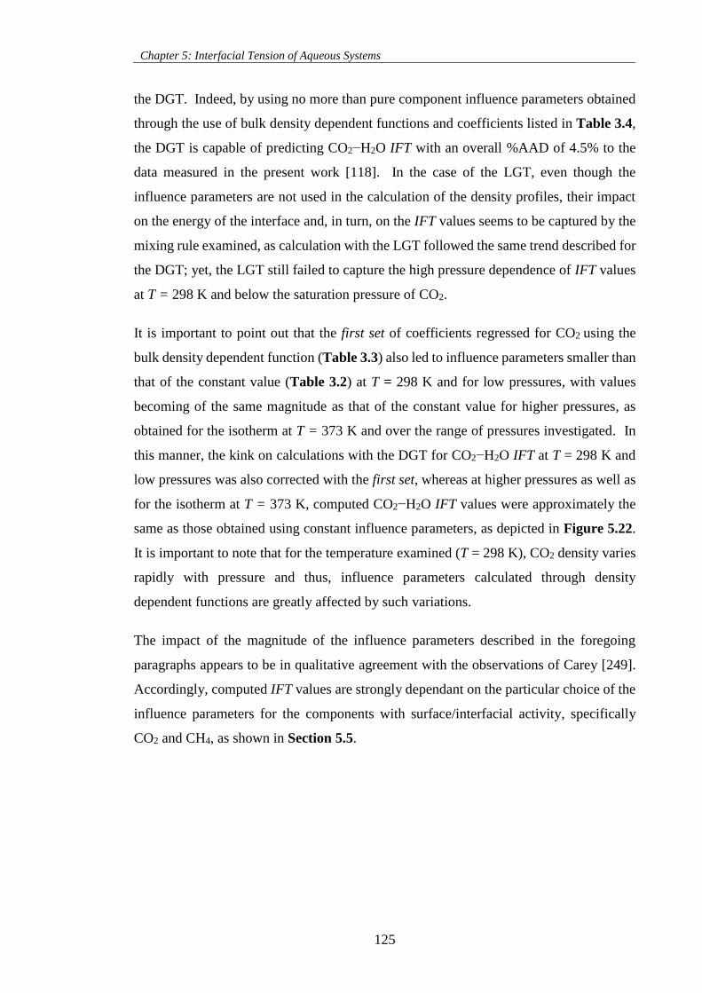
Chapter 5: Interfacial Tension of Aqueous Systems
125
the DGT. Indeed, by using no more than pure component influence parameters obtained
through the use of bulk density dependent functions and coefficients listed in Table 3.4,
the DGT is capable of predicting CO2−H2O IFT with an overall %AAD of 4.5% to the
data measured in the present work [118]. In the case of the LGT, even though the
influence parameters are not used in the calculation of the density profiles, their impact
on the energy of the interface and, in turn, on the IFT values seems to be captured by the
mixing rule examined, as calculation with the LGT followed the same trend described for
the DGT; yet, the LGT still failed to capture the high pressure dependence of IFT values
at T = 298 K and below the saturation pressure of CO2.
It is important to point out that the first set of coefficients regressed for CO2 using the
bulk density dependent function (Table 3.3) also led to influence parameters smaller than
that of the constant value (Table 3.2) at T = 298 K and for low pressures, with values
becoming of the same magnitude as that of the constant value for higher pressures, as
obtained for the isotherm at T = 373 K and over the range of pressures investigated. In
this manner, the kink on calculations with the DGT for CO2−H2O IFT at T = 298 K and
low pressures was also corrected with the first set, whereas at higher pressures as well as
for the isotherm at T = 373 K, computed CO2−H2O IFT values were approximately the
same as those obtained using constant influence parameters, as depicted in Figure 5.22.
It is important to note that for the temperature examined (T = 298 K), CO2 density varies
rapidly with pressure and thus, influence parameters calculated through density
dependent functions are greatly affected by such variations.
The impact of the magnitude of the influence parameters described in the foregoing
paragraphs appears to be in qualitative agreement with the observations of Carey [249].
Accordingly, computed IFT values are strongly dependant on the particular choice of the
influence parameters for the components with surface/interfacial activity, specifically
CO2 and CH4, as shown in Section 5.5.
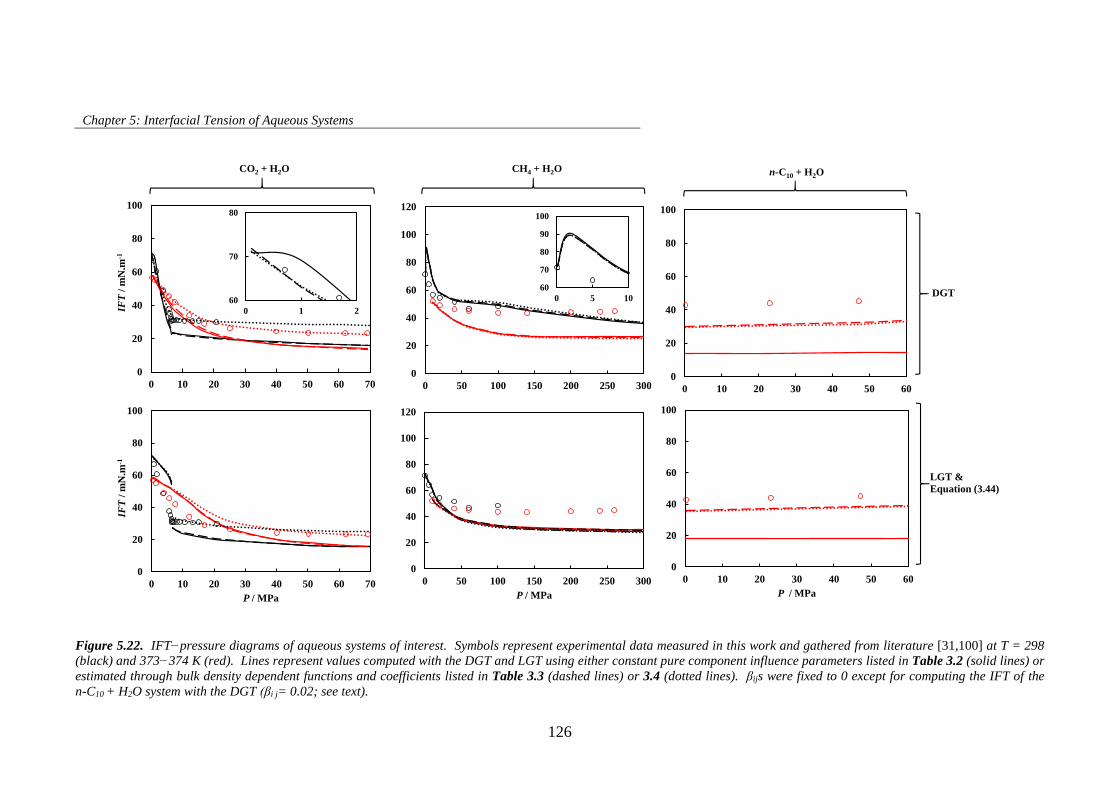
Chapter 5: Interfacial Tension of Aqueous Systems
126
Figure 5.22. IFT−pressure diagrams of aqueous systems of interest. Symbols represent experimental data measured in this work and gathered from literature [31,100] at T = 298
(black) and 373−374 K (red). Lines represent values computed with the DGT and LGT using either constant pure component influence parameters listed in Table 3.2 (solid lines) or
estimated through bulk density dependent functions and coefficients listed in Table 3.3 (dashed lines) or 3.4 (dotted lines). βijs were fixed to 0 except for computing the IFT of the
n-C10 + H2O system with the DGT (βi j= 0.02; see text).
0
20
40
60
80
100
0 10 20 30 40 50 60 70
IFT
/ m
N.m
-1
0
20
40
60
80
100
120
0 50 100 150 200 250 3000
20
40
60
80
100
0 10 20 30 40 50 60
0
20
40
60
80
100
0 10 20 30 40 50 60 70
IFT
/ m
N.m
-1
P / MPa
0
20
40
60
80
100
120
0 50 100 150 200 250 300
P / MPa
0
20
40
60
80
100
0 10 20 30 40 50 60
P / MPa
60
70
80
0 1 2
n-C10 + H2O
DGT
LGT &
Equation (3.44)
CH4 + H2OCO2 + H2O
60
70
80
90
100
0 5 10
Chapter 5: Interfacial Tension of Aqueous Systems
127
Based on what has been described, the better agreement of DGT and LGT calculations to
experimental data appears to be intrinsically associated with the value of influence
parameters of the non-aqueous components. In the case of CO2 and n-C10, they were
positively estimated through the use of bulk density dependent functions together with
specific set of coefficients regressed against surface tension data. Furthermore, the
influence parameters were estimated using pure component properties in the subcritical
region which, in turn, may not be enough for providing an accurate representation of the
influence parameters at/or above supercritical conditions, specifically for CO2 (Tc ~ 304
K) and CH4 (Tc ~ 190 K). As a result, the characteristics of the interface as well as the
IFT are not correctly described. To circumvent this constraint, it was decided to use
henceforth only constant values for the influence parameters of all pure components
(Table 3.2) and the IFT of binary systems corrected using a value for βij ≠ 0. This
procedure is in line with that followed by many others [217–219,222,250] when
modelling such challenging systems.
In order to keep the number of adjustable parameters at a minimum, βijs were estimated
with the help of one experimental IFT data point of each of the binary systems examined,
at moderate pressure and temperature conditions, and then used to compute the IFT at
other conditions. The values of βij used are listed in Table 5.6 along with the %AAD of
computed values with the DGT and LGT to experimental IFT data. A graphical
representation of the results is provided in Figures 5.23 and 5.24 for selected isotherms.
Calculations using Sutton’s correlation have also been included in the figures to allow
some discussion as well as deviations to experimental IFT data in Table 5.6; under this
approach, the required density difference was calculated from pure component density
[99,344], as followed by Sutton [178]. Even though Sutton [178] did not use IFT data for
CO2 + H2O and N2 + H2O in his model development, deviations from this approach to
IFT experiments for these systems are also provided.
From Figures 5.23 and 5.24 it can be observed that the DGT gave the best IFT
estimations, with an overall %AAD to experiments of 4.2% (Table 5.6). The use of a
single binary interaction coefficient between influence parameters helped to improve
significantly IFT estimations as well as to correct the behaviour described at low pressures
(i.e., kink). These modelling results are in agreement with that of others. For example,
Niño-Amezquita and co-workers [219,222] coupled the DGT with the PC-SAFT EoS and
modelled the IFT of CO2 + H2O, up to T = 333 K and P = 25 MPa, using βij = 0.75 and
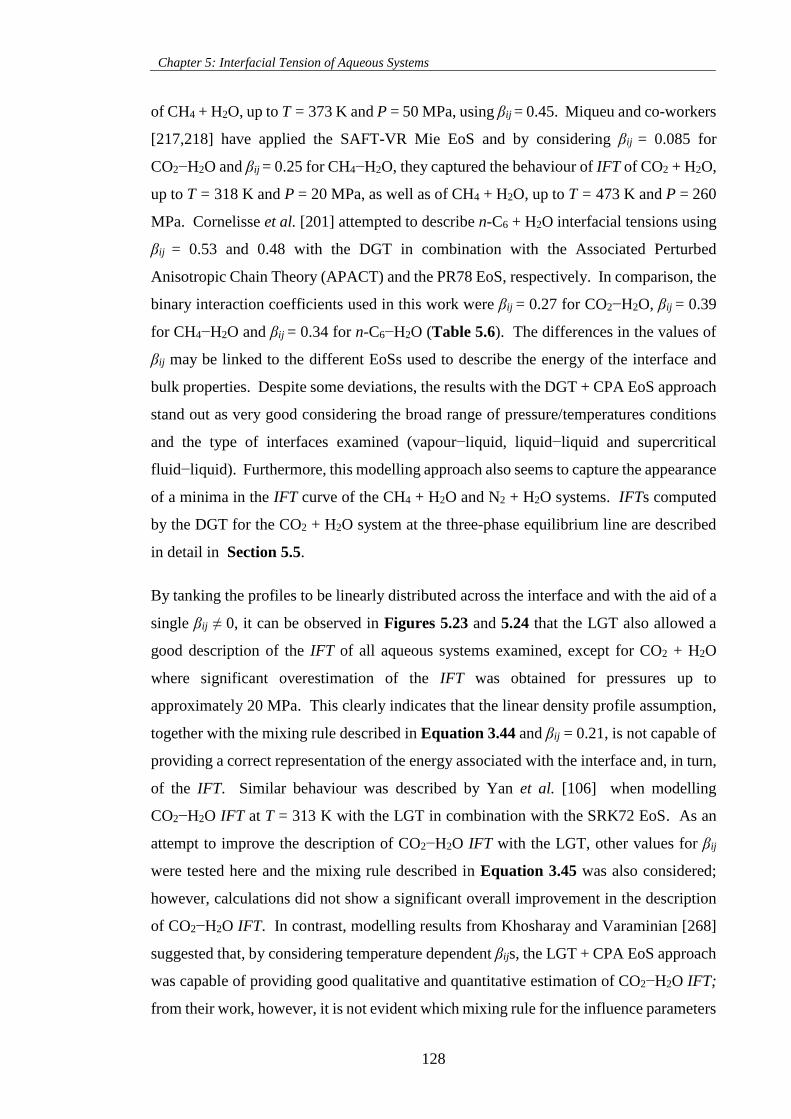
Chapter 5: Interfacial Tension of Aqueous Systems
128
of CH4 + H2O, up to T = 373 K and P = 50 MPa, using βij = 0.45. Miqueu and co-workers
[217,218] have applied the SAFT-VR Mie EoS and by considering βij = 0.085 for
CO2−H2O and βij = 0.25 for CH4−H2O, they captured the behaviour of IFT of CO2 + H2O,
up to T = 318 K and P = 20 MPa, as well as of CH4 + H2O, up to T = 473 K and P = 260
MPa. Cornelisse et al. [201] attempted to describe n-C6 + H2O interfacial tensions using
βij = 0.53 and 0.48 with the DGT in combination with the Associated Perturbed
Anisotropic Chain Theory (APACT) and the PR78 EoS, respectively. In comparison, the
binary interaction coefficients used in this work were βij = 0.27 for CO2−H2O, βij = 0.39
for CH4−H2O and βij = 0.34 for n-C6−H2O (Table 5.6). The differences in the values of
βij may be linked to the different EoSs used to describe the energy of the interface and
bulk properties. Despite some deviations, the results with the DGT + CPA EoS approach
stand out as very good considering the broad range of pressure/temperatures conditions
and the type of interfaces examined (vapour−liquid, liquid−liquid and supercritical
fluid−liquid). Furthermore, this modelling approach also seems to capture the appearance
of a minima in the IFT curve of the CH4 + H2O and N2 + H2O systems. IFTs computed
by the DGT for the CO2 + H2O system at the three-phase equilibrium line are described
in detail in Section 5.5.
By tanking the profiles to be linearly distributed across the interface and with the aid of a
single βij ≠ 0, it can be observed in Figures 5.23 and 5.24 that the LGT also allowed a
good description of the IFT of all aqueous systems examined, except for CO2 + H2O
where significant overestimation of the IFT was obtained for pressures up to
approximately 20 MPa. This clearly indicates that the linear density profile assumption,
together with the mixing rule described in Equation 3.44 and βij = 0.21, is not capable of
providing a correct representation of the energy associated with the interface and, in turn,
of the IFT. Similar behaviour was described by Yan et al. [106] when modelling
CO2−H2O IFT at T = 313 K with the LGT in combination with the SRK72 EoS. As an
attempt to improve the description of CO2−H2O IFT with the LGT, other values for βij
were tested here and the mixing rule described in Equation 3.45 was also considered;
however, calculations did not show a significant overall improvement in the description
of CO2−H2O IFT. In contrast, modelling results from Khosharay and Varaminian [268]
suggested that, by considering temperature dependent βijs, the LGT + CPA EoS approach
was capable of providing good qualitative and quantitative estimation of CO2−H2O IFT;
from their work, however, it is not evident which mixing rule for the influence parameters
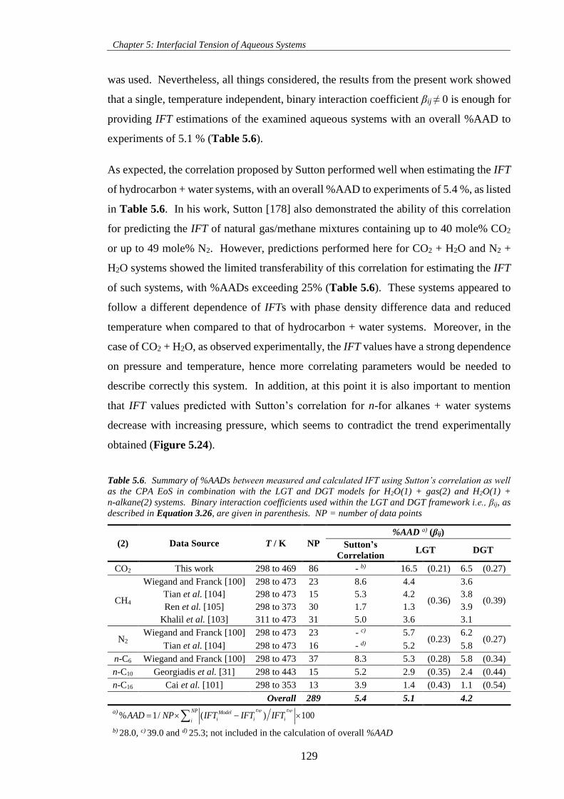
Chapter 5: Interfacial Tension of Aqueous Systems
129
was used. Nevertheless, all things considered, the results from the present work showed
that a single, temperature independent, binary interaction coefficient βij ≠ 0 is enough for
providing IFT estimations of the examined aqueous systems with an overall %AAD to
experiments of 5.1 % (Table 5.6).
As expected, the correlation proposed by Sutton performed well when estimating the IFT
of hydrocarbon + water systems, with an overall %AAD to experiments of 5.4 %, as listed
in Table 5.6. In his work, Sutton [178] also demonstrated the ability of this correlation
for predicting the IFT of natural gas/methane mixtures containing up to 40 mole% CO2
or up to 49 mole% N2. However, predictions performed here for CO2 + H2O and N2 +
H2O systems showed the limited transferability of this correlation for estimating the IFT
of such systems, with %AADs exceeding 25% (Table 5.6). These systems appeared to
follow a different dependence of IFTs with phase density difference data and reduced
temperature when compared to that of hydrocarbon + water systems. Moreover, in the
case of CO2 + H2O, as observed experimentally, the IFT values have a strong dependence
on pressure and temperature, hence more correlating parameters would be needed to
describe correctly this system. In addition, at this point it is also important to mention
that IFT values predicted with Sutton’s correlation for n-for alkanes + water systems
decrease with increasing pressure, which seems to contradict the trend experimentally
obtained (Figure 5.24).
Table 5.6. Summary of %AADs between measured and calculated IFT using Sutton’s correlation as well
as the CPA EoS in combination with the LGT and DGT models for H2O(1) + gas(2) and H2O(1) +
n-alkane(2) systems. Binary interaction coefficients used within the LGT and DGT framework i.e., βij, as
described in Equation 3.26, are given in parenthesis. NP = number of data points
(2) Data Source T / K NP
%AAD a) (βij)
Sutton’s
Correlation LGT DGT
CO2 This work 298 to 469 86 - b) 16.5 (0.21) 6.5 (0.27)
CH4
Wiegand and Franck [100] 298 to 473 23 8.6 4.4
(0.36)
3.6
(0.39) Tian et al. [104] 298 to 473 15 5.3 4.2 3.8
Ren et al. [105] 298 to 373 30 1.7 1.3 3.9
Khalil et al. [103] 311 to 473 31 5.0 3.6 3.1
N2 Wiegand and Franck [100] 298 to 473 23 - c) 5.7
(0.23) 6.2
(0.27) Tian et al. [104] 298 to 473 16 - d) 5.2 5.8
n-C6 Wiegand and Franck [100] 298 to 473 37 8.3 5.3 (0.28) 5.8 (0.34)
n-C10 Georgiadis et al. [31] 298 to 443 15 5.2 2.9 (0.35) 2.4 (0.44)
n-C16 Cai et al. [101] 298 to 353 13 3.9 1.4 (0.43) 1.1 (0.54)
Overall 289 5.4 5.1 4.2
a)% 1/ ( ) 100
Exp ExpNP Model
i i iiAAD NP IFT IFT IFT
b) 28.0, c) 39.0 and d) 25.3; not included in the calculation of overall %AAD
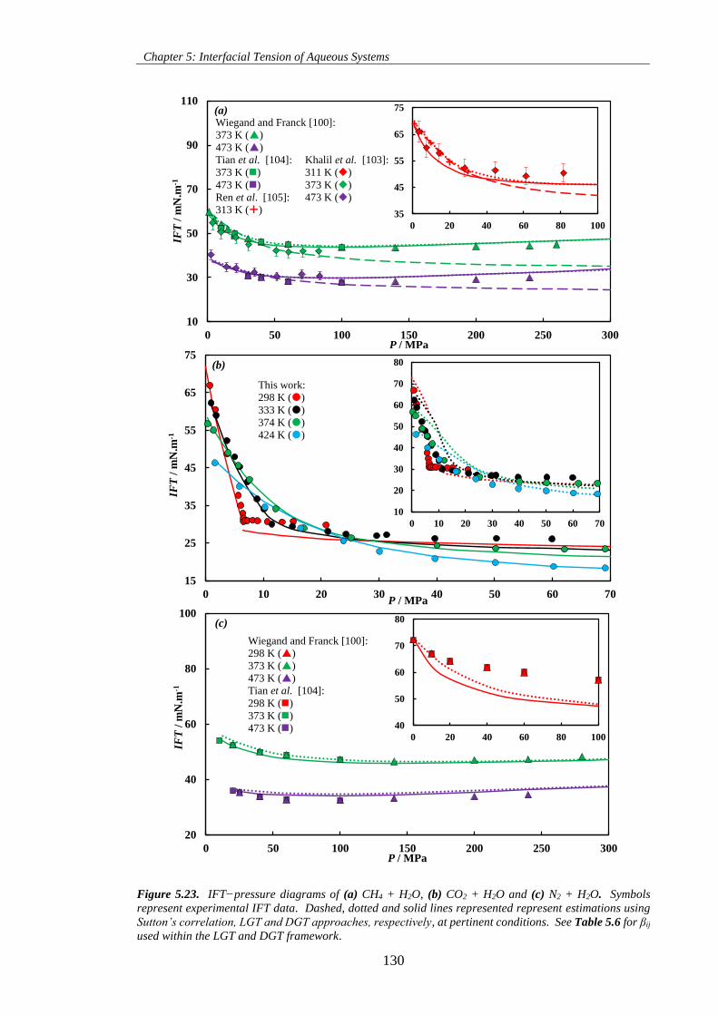
Chapter 5: Interfacial Tension of Aqueous Systems
130
Figure 5.23. IFT−pressure diagrams of (a) CH4 + H2O, (b) CO2 + H2O and (c) N2 + H2O. Symbols
represent experimental IFT data. Dashed, dotted and solid lines represented represent estimations using
Sutton’s correlation, LGT and DGT approaches, respectively, at pertinent conditions. See Table 5.6 for βij
used within the LGT and DGT framework.
20
40
60
80
100
0 50 100 150 200 250 300
IFT
/ m
N.m
-1
P / MPa
40
50
60
70
80
0 20 40 60 80 100
10
30
50
70
90
110
0 50 100 150 200 250 300
IFT
/ m
N.m
-1
P / MPa
35
45
55
65
75
0 20 40 60 80 100
15
25
35
45
55
65
75
0 10 20 30 40 50 60 70
IFT
/ m
N.m
-1
P / MPa
10
20
30
40
50
60
70
80
0 10 20 30 40 50 60 70
(a)
(b)
(c)
Wiegand and Franck [100]:
373 K ()
473 K ()
Tian et al. [104]: Khalil et al. [103]:
373 K () 311 K ()
473 K () 373 K ()
Ren et al. [105]: 473 K ()
313 K ()
Wiegand and Franck [100]:
298 K ()
373 K ()
473 K ()
Tian et al. [104]:
298 K ()
373 K ()
473 K ()
This work:
298 K ()
333 K ()
374 K ()
424 K ()
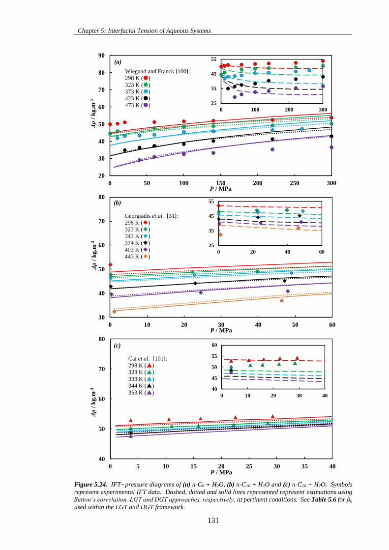
Chapter 5: Interfacial Tension of Aqueous Systems
131
Figure 5.24. IFT−pressure diagrams of (a) n-C6 + H2O, (b) n-C10 + H2O and (c) n-C16 + H2O. Symbols
represent experimental IFT data. Dashed, dotted and solid lines represented represent estimations using
Sutton’s correlation, LGT and DGT approaches, respectively, at pertinent conditions. See Table 5.6 for βij
used within the LGT and DGT framework.
20
30
40
50
60
70
80
90
0 50 100 150 200 250 300
Δρ
/ k
g.m
-3
P / MPa
298 K 323 K
373 K 423 K
473 K 25
35
45
55
0 100 200 300
30
40
50
60
70
80
0 10 20 30 40 50 60
Δρ
/ k
g.m
-3
P / MPa
298 K
323 K
343 K
374 K
403 K
443 K
25
35
45
55
0 20 40 60
(b)
(a)
40
50
60
70
80
0 5 10 15 20 25 30 35 40
Δρ
/ k
g.m
-3
P / MPa
298 K
323 K
333 K
343 K
353 K40
45
50
55
60
0 10 20 30 40
(c)
Wiegand and Franck [100]:
298 K ()
323 K ()
373 K ()
423 K ()
473 K ()
Georgiadis et al. [31]:
298 K ()
323 K ()
343 K ()
374 K ()
403 K ()
443 K ()
Cai et al. [101]:
298 K ()
323 K ()
333 K ()
344 K ()
353 K ()
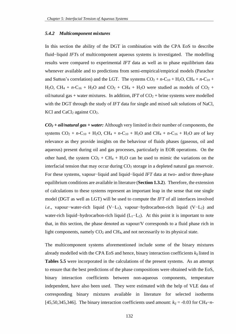
Chapter 5: Interfacial Tension of Aqueous Systems
132
5.4.2 Multicomponent mixtures
In this section the ability of the DGT in combination with the CPA EoS to describe
fluid−liquid IFTs of multicomponent aqueous systems is investigated. The modelling
results were compared to experimental IFT data as well as to phase equilibrium data
whenever available and to predictions from semi-empirical/empirical models (Parachor
and Sutton’s correlation) and the LGT. The systems CO2 + n-C10 + H2O, CH4 + n-C10 +
H2O, CH4 + n-C16 + H2O and CO2 + CH4 + H2O were studied as models of CO2 +
oil/natural gas + water mixtures. In addition, IFT of CO2 + brine systems were modelled
with the DGT through the study of IFT data for single and mixed salt solutions of NaCl,
KCl and CaCl2 against CO2.
CO2 + oil/natural gas + water: Although very limited in their number of components, the
systems CO2 + n-C10 + H2O, CH4 + n-C10 + H2O and CH4 + n-C16 + H2O are of key
relevance as they provide insights on the behaviour of fluids phases (gaseous, oil and
aqueous) present during oil and gas processes, particularly in EOR operations. On the
other hand, the system CO2 + CH4 + H2O can be used to mimic the variations on the
interfacial tension that may occur during CO2 storage in a depleted natural gas reservoir.
For these systems, vapour−liquid and liquid−liquid IFT data at two- and/or three-phase
equilibrium conditions are available in literature (Section 1.3.2). Therefore, the extension
of calculations to these systems represent an important leap in the sense that one single
model (DGT as well as LGT) will be used to compute the IFT of all interfaces involved
i.e., vapour−water-rich liquid (V−L1), vapour−hydrocarbon-rich liquid (V−L2) and
water-rich liquid−hydrocarbon-rich liquid (L1−L2). At this point it is important to note
that, in this section, the phase denoted as vapour/V corresponds to a fluid phase rich in
light components, namely CO2 and CH4, and not necessarily to its physical state.
The multicomponent systems aforementioned include some of the binary mixtures
already modelled with the CPA EoS and hence, binary interaction coefficients kij listed in
Tables 5.5 were incorporated in the calculations of the present systems. As an attempt
to ensure that the best predictions of the phase compositions were obtained with the EoS,
binary interaction coefficients between non-aqueous components, temperature
independent, have also been used. They were estimated with the help of VLE data of
corresponding binary mixtures available in literature for selected isotherms
[45,50,345,346]. The binary interaction coefficients used amount: kij = -0.03 for CH4−n-
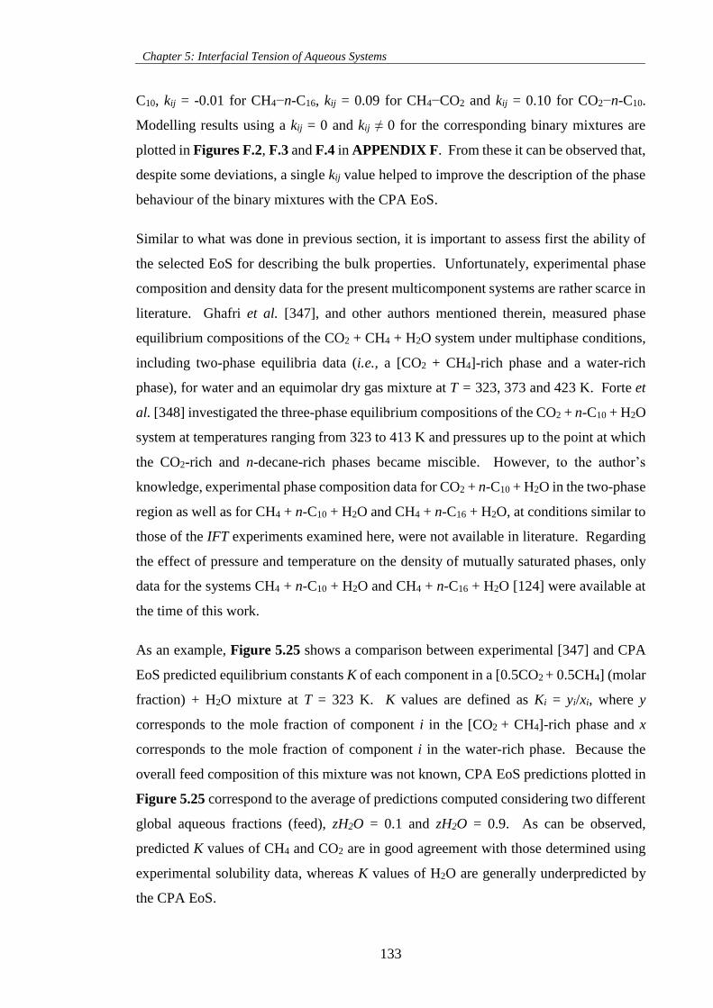
Chapter 5: Interfacial Tension of Aqueous Systems
133
C10, kij = -0.01 for CH4−n-C16, kij = 0.09 for CH4−CO2 and kij = 0.10 for CO2−n-C10.
Modelling results using a kij = 0 and kij ≠ 0 for the corresponding binary mixtures are
plotted in Figures F.2, F.3 and F.4 in APPENDIX F. From these it can be observed that,
despite some deviations, a single kij value helped to improve the description of the phase
behaviour of the binary mixtures with the CPA EoS.
Similar to what was done in previous section, it is important to assess first the ability of
the selected EoS for describing the bulk properties. Unfortunately, experimental phase
composition and density data for the present multicomponent systems are rather scarce in
literature. Ghafri et al. [347], and other authors mentioned therein, measured phase
equilibrium compositions of the CO2 + CH4 + H2O system under multiphase conditions,
including two-phase equilibria data (i.e., a [CO2 + CH4]-rich phase and a water-rich
phase), for water and an equimolar dry gas mixture at T = 323, 373 and 423 K. Forte et
al. [348] investigated the three-phase equilibrium compositions of the CO2 + n-C10 + H2O
system at temperatures ranging from 323 to 413 K and pressures up to the point at which
the CO2-rich and n-decane-rich phases became miscible. However, to the author’s
knowledge, experimental phase composition data for CO2 + n-C10 + H2O in the two-phase
region as well as for CH4 + n-C10 + H2O and CH4 + n-C16 + H2O, at conditions similar to
those of the IFT experiments examined here, were not available in literature. Regarding
the effect of pressure and temperature on the density of mutually saturated phases, only
data for the systems CH4 + n-C10 + H2O and CH4 + n-C16 + H2O [124] were available at
the time of this work.
As an example, Figure 5.25 shows a comparison between experimental [347] and CPA
EoS predicted equilibrium constants K of each component in a [0.5CO2 + 0.5CH4] (molar
fraction) + H2O mixture at T = 323 K. K values are defined as Ki = yi/xi, where y
corresponds to the mole fraction of component i in the [CO2 + CH4]-rich phase and x
corresponds to the mole fraction of component i in the water-rich phase. Because the
overall feed composition of this mixture was not known, CPA EoS predictions plotted in
Figure 5.25 correspond to the average of predictions computed considering two different
global aqueous fractions (feed), zH2O = 0.1 and zH2O = 0.9. As can be observed,
predicted K values of CH4 and CO2 are in good agreement with those determined using
experimental solubility data, whereas K values of H2O are generally underpredicted by
the CPA EoS.
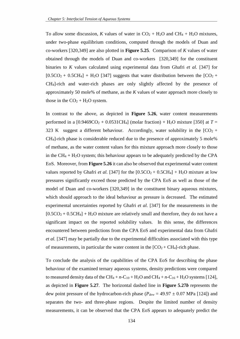
Chapter 5: Interfacial Tension of Aqueous Systems
134
To allow some discussion, K values of water in CO2 + H2O and CH4 + H2O mixtures,
under two-phase equilibrium conditions, computed through the models of Duan and
co-workers [320,349] are also plotted in Figure 5.25. Comparison of K values of water
obtained through the models of Duan and co-workers [320,349] for the constituent
binaries to K values calculated using experimental data from Ghafri et al. [347] for
[0.5CO2 + 0.5CH4] + H2O [347] suggests that water distribution between the [CO2 +
CH4]-rich and water-rich phases are only slightly affected by the presence of
approximately 50 mole% of methane, as the K values of water approach more closely to
those in the CO2 + H2O system.
In contrast to the above, as depicted in Figure 5.26, water content measurements
performed in a [0.9469CO2 + 0.0531CH4] (molar fraction) + H2O mixture [350] at T =
323 K suggest a different behaviour. Accordingly, water solubility in the [CO2 +
CH4]-rich phase is considerable reduced due to the presence of approximately 5 mole%
of methane, as the water content values for this mixture approach more closely to those
in the CH4 + H2O system; this behaviour appears to be adequately predicted by the CPA
EoS. Moreover, from Figure 5.26 it can also be observed that experimental water content
values reported by Ghafri et al. [347] for the [0.5CO2 + 0.5CH4] + H2O mixture at low
pressures significantly exceed those predicted by the CPA EoS as well as those of the
model of Duan and co-workers [320,349] in the constituent binary aqueous mixtures,
which should approach to the ideal behaviour as pressure is decreased. The estimated
experimental uncertainties reported by Ghafri et al. [347] for the measurements in the
[0.5CO2 + 0.5CH4] + H2O mixture are relatively small and therefore, they do not have a
significant impact on the reported solubility values. In this sense, the differences
encountered between predictions from the CPA EoS and experimental data from Ghafri
et al. [347] may be partially due to the experimental difficulties associated with this type
of measurements, in particular the water content in the [CO2 + CH4]-rich phase.
To conclude the analysis of the capabilities of the CPA EoS for describing the phase
behaviour of the examined ternary aqueous systems, density predictions were compared
to measured density data of the CH4 + n-C10 + H2O and CH4 + n-C16 + H2O systems [124],
as depicted in Figure 5.27. The horizontal dashed line in Figure 5.27b represents the
dew point pressure of the hydrocarbon-rich phase (Pdew = 49.97 ± 0.07 MPa [124]) and
separates the two- and three-phase regions. Despite the limited number of density
measurements, it can be observed that the CPA EoS appears to adequately predict the
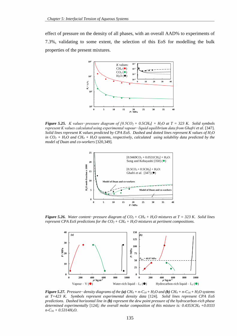
Chapter 5: Interfacial Tension of Aqueous Systems
135
effect of pressure on the density of all phases, with an overall AAD% to experiments of
7.3%, validating to some extent, the selection of this EoS for modelling the bulk
properties of the present mixtures.
Figure 5.25. K values−pressure diagram of [0.5CO2 + 0.5CH4] + H2O at T = 323 K. Solid symbols
represent K values calculated using experimental vapour−liquid equilibrium data from Ghafri et al. [347].
Solid lines represent K values predicted by CPA EoS. Dashed and dotted lines represent K values of H2O
in CO2 + H2O and CH4 + H2O systems, respectively, calculated using solubility data predicted by the
model of Duan and co-workers [320,349].
Figure 5.26. Water content−pressure diagram of CO2 + CH4 + H2O mixtures at T = 323 K. Solid lines
represent CPA EoS predictions for the CO2 + CH4 + H2O mixtures at pertinent compositions.
Figure 5.27. Pressure−density diagrams of the (a) CH4 + n-C10 + H2O and (b) CH4 + n-C16 + H2O systems
at T=423 K. Symbols represent experimental density data [124]. Solid lines represent CPA EoS
predictions. Dashed horizontal line in (b) represent the dew point pressure of the hydrocarbon-rich phase
determined experimentally [124]; the overall molar composition of this mixture is: 0.4353CH4 +0.0333
n-C16 + 0.5314H2O.
10
100
1000
10000
0 5 10 15 20 25 30 35 40
Ki=
yi/x
i
P / MPa
0.00
0.00
0.01
0.10
0 10 20 30 40
104
103
102
101
10-1
10-2
10-3
10-3
10-4
0
5
10
15
20
25
0 5 10 15 20 25 30 35 40
H2O
mole
fra
ctio
n x
1000
P / MPa
Model of Duan and co-workers
Model of Duan and co-workers
0
25
50
75
100
125
150
0 200 400 600 800 1000
P /
MP
a
ρ/ kg.m-3
0
10
20
30
40
0 200 400 600 800 1000
P /
MP
a
ρ/ kg.m-3
(a) (b)
Pdew = 49.97 MPa
Vapour – V () Water-rich liquid – L1 () Hydrocarbon-rich liquid – L2 ()
[0.9469CO2 + 0.0531CH4] + H2O: Song and Kobayashi [350] ()
[0.5CO2 + 0.5CH4] + H2O:
Ghafri et al. [347] ()
K values:
CH4 () CO2 ()
H2O ()
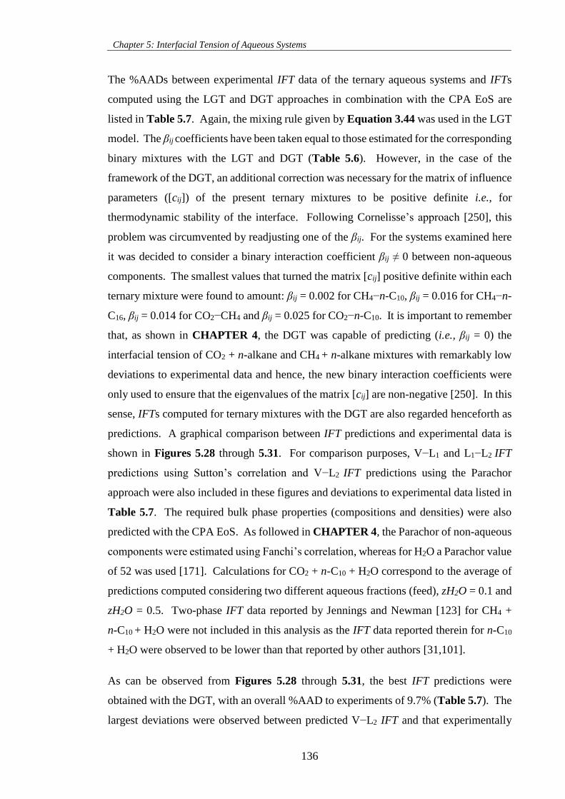
Chapter 5: Interfacial Tension of Aqueous Systems
136
The %AADs between experimental IFT data of the ternary aqueous systems and IFTs
computed using the LGT and DGT approaches in combination with the CPA EoS are
listed in Table 5.7. Again, the mixing rule given by Equation 3.44 was used in the LGT
model. The βij coefficients have been taken equal to those estimated for the corresponding
binary mixtures with the LGT and DGT (Table 5.6). However, in the case of the
framework of the DGT, an additional correction was necessary for the matrix of influence
parameters ([cij]) of the present ternary mixtures to be positive definite i.e., for
thermodynamic stability of the interface. Following Cornelisse’s approach [250], this
problem was circumvented by readjusting one of the βij. For the systems examined here
it was decided to consider a binary interaction coefficient βij ≠ 0 between non-aqueous
components. The smallest values that turned the matrix [cij] positive definite within each
ternary mixture were found to amount: βij = 0.002 for CH4−n-C10, βij = 0.016 for CH4−n-
C16, βij = 0.014 for CO2−CH4 and βij = 0.025 for CO2−n-C10. It is important to remember
that, as shown in CHAPTER 4, the DGT was capable of predicting (i.e., βij = 0) the
interfacial tension of CO2 + n-alkane and CH4 + n-alkane mixtures with remarkably low
deviations to experimental data and hence, the new binary interaction coefficients were
only used to ensure that the eigenvalues of the matrix [cij] are non-negative [250]. In this
sense, IFTs computed for ternary mixtures with the DGT are also regarded henceforth as
predictions. A graphical comparison between IFT predictions and experimental data is
shown in Figures 5.28 through 5.31. For comparison purposes, V−L1 and L1−L2 IFT
predictions using Sutton’s correlation and V−L2 IFT predictions using the Parachor
approach were also included in these figures and deviations to experimental data listed in
Table 5.7. The required bulk phase properties (compositions and densities) were also
predicted with the CPA EoS. As followed in CHAPTER 4, the Parachor of non-aqueous
components were estimated using Fanchi’s correlation, whereas for H2O a Parachor value
of 52 was used [171]. Calculations for CO2 + n-C10 + H2O correspond to the average of
predictions computed considering two different aqueous fractions (feed), zH2O = 0.1 and
zH2O = 0.5. Two-phase IFT data reported by Jennings and Newman [123] for CH4 +
n-C10 + H2O were not included in this analysis as the IFT data reported therein for n-C10
+ H2O were observed to be lower than that reported by other authors [31,101].
As can be observed from Figures 5.28 through 5.31, the best IFT predictions were
obtained with the DGT, with an overall %AAD to experiments of 9.7% (Table 5.7). The
largest deviations were observed between predicted V−L2 IFT and that experimentally
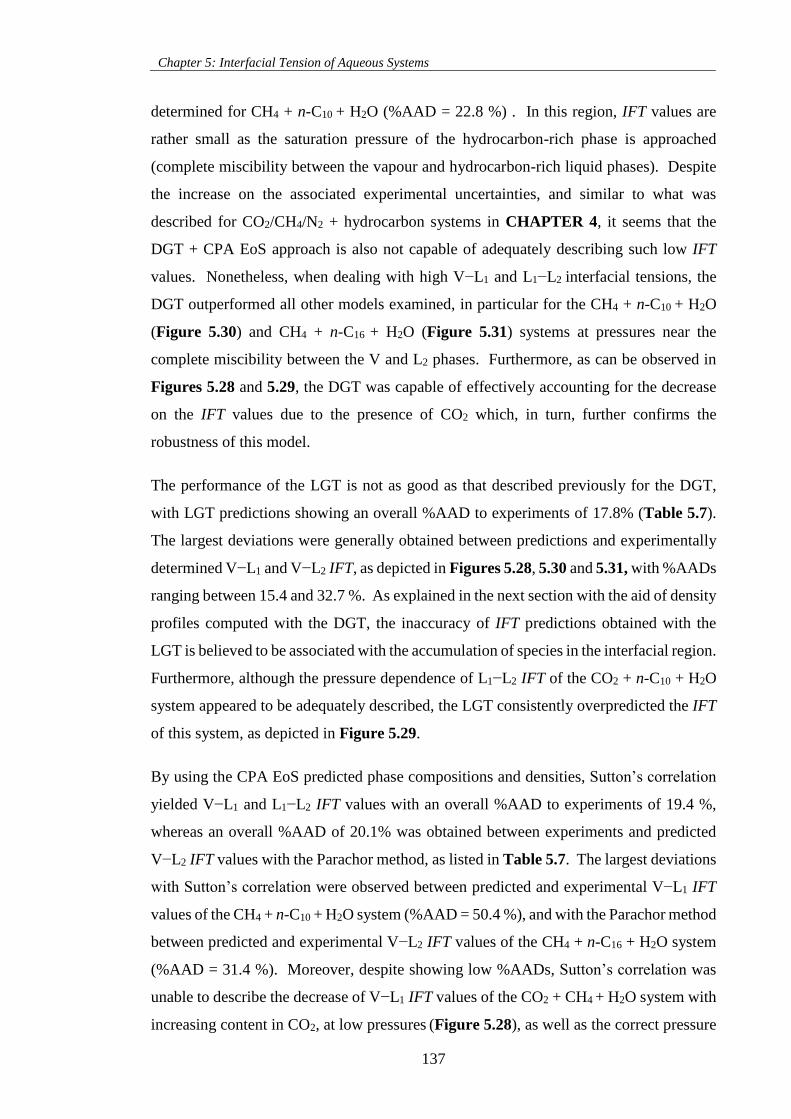
Chapter 5: Interfacial Tension of Aqueous Systems
137
determined for CH4 + n-C10 + H2O (%AAD = 22.8 %) . In this region, IFT values are
rather small as the saturation pressure of the hydrocarbon-rich phase is approached
(complete miscibility between the vapour and hydrocarbon-rich liquid phases). Despite
the increase on the associated experimental uncertainties, and similar to what was
described for CO2/CH4/N2 + hydrocarbon systems in CHAPTER 4, it seems that the
DGT + CPA EoS approach is also not capable of adequately describing such low IFT
values. Nonetheless, when dealing with high V−L1 and L1−L2 interfacial tensions, the
DGT outperformed all other models examined, in particular for the CH4 + n-C10 + H2O
(Figure 5.30) and CH4 + n-C16 + H2O (Figure 5.31) systems at pressures near the
complete miscibility between the V and L2 phases. Furthermore, as can be observed in
Figures 5.28 and 5.29, the DGT was capable of effectively accounting for the decrease
on the IFT values due to the presence of CO2 which, in turn, further confirms the
robustness of this model.
The performance of the LGT is not as good as that described previously for the DGT,
with LGT predictions showing an overall %AAD to experiments of 17.8% (Table 5.7).
The largest deviations were generally obtained between predictions and experimentally
determined V−L1 and V−L2 IFT, as depicted in Figures 5.28, 5.30 and 5.31, with %AADs
ranging between 15.4 and 32.7 %. As explained in the next section with the aid of density
profiles computed with the DGT, the inaccuracy of IFT predictions obtained with the
LGT is believed to be associated with the accumulation of species in the interfacial region.
Furthermore, although the pressure dependence of L1−L2 IFT of the CO2 + n-C10 + H2O
system appeared to be adequately described, the LGT consistently overpredicted the IFT
of this system, as depicted in Figure 5.29.
By using the CPA EoS predicted phase compositions and densities, Sutton’s correlation
yielded V−L1 and L1−L2 IFT values with an overall %AAD to experiments of 19.4 %,
whereas an overall %AAD of 20.1% was obtained between experiments and predicted
V−L2 IFT values with the Parachor method, as listed in Table 5.7. The largest deviations
with Sutton’s correlation were observed between predicted and experimental V−L1 IFT
values of the CH4 + n-C10 + H2O system (%AAD = 50.4 %), and with the Parachor method
between predicted and experimental V−L2 IFT values of the CH4 + n-C16 + H2O system
(%AAD = 31.4 %). Moreover, despite showing low %AADs, Sutton’s correlation was
unable to describe the decrease of V−L1 IFT values of the CO2 + CH4 + H2O system with
increasing content in CO2, at low pressures (Figure 5.28), as well as the correct pressure
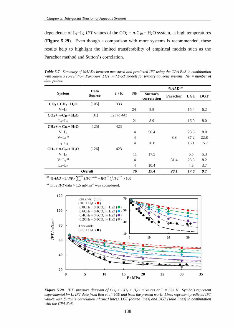
Chapter 5: Interfacial Tension of Aqueous Systems
138
dependence of L1−L2 IFT values of the CO2 + n-C10 + H2O system, at high temperatures
(Figure 5.29). Even though a comparison with more systems is recommended, these
results help to highlight the limited transferability of empirical models such as the
Parachor method and Sutton’s correlation.
Table 5.7. Summary of %AADs between measured and predicted IFT using the CPA EoS in combination
with Sutton’s correlation, Parachor, LGT and DGT models for ternary aqueous systems. NP = number of
data points.
System Data
Source T / K NP
%AAD a)
Sutton's
correlation Parachor LGT DGT
CO2 + CH4+ H2O [105] 333
V−L1 24 8.8 15.4 6.2
CO2 + n-C10 + H2O [31] 323 to 443
L1−L2 21 8.9 16.0 8.0
CH4 + n-C10 + H2O [125] 423
V−L1 4 50.4 23.6 8.0
V−L2 b) 4 8.8 37.2 22.8
L1−L2 4 20.8 16.1 15.7
CH4 + n-C16 + H2O [126] 423
V−L1 11 17.5 6.5 5.3
V−L2 b) 4 31.4 23.3 8.2
L1−L2 4 10.4 4.5 3.7
Overall 76 19.4 20.1 17.8 9.7
a) % 1/ ( ) 100
Exp ExpNP Model
i i iiAAD NP IFT IFT IFT
b) Only IFT data > 1.5 mN.m-1 was considered.
Figure 5.28. IFT−pressure diagram of CO2 + CH4 + H2O mixtures at T = 333 K. Symbols represent
experimental V−L1 IFT data from Ren et al.[105] and from the present work. Lines represent predicted IFT
values with Sutton’s correlation (dashed lines), LGT (dotted lines) and DGT (solid lines) in combination
with the CPA EoS.
20
40
60
80
100
120
0 5 10 15 20 25 30 35
IFT
/ m
N.m
-1
P / MPa
10
30
50
70
0 10 20 30
Ren et al. [105]:
CH4 + H2O ()
[0.8CH4 + 0.2CO2] + H2O ()
[0.6CH4 + 0.4CO2] + H2O ()
[0.4CH4 + 0.6CO2] + H2O ()
[0.2CH4 + 0.8CO2] + H2O ()
This work:
CO2 + H2O ()
Chapter 5: Interfacial Tension of Aqueous Systems
139
Figure 5.29. IFT−pressure diagrams of (a) [0.2 CO2 + 0.8n-C10] + H2O and (b) [0.5 CO2 + 0.5n-C10] +
H2O (b) mixtures. Solid symbols represent experimental L1−L2 IFT data [31]. Lines represent predicted
IFT values with Sutton’s correlation (dashed lines), LGT (dotted lines) and DGT (solid lines) models in
combination with the CPA EoS.
Figure 5.30. IFT−pressure diagrams of the CH4 + n-C10 + H2O system at T = 423 K. Solid symbols
represent experimental IFT data [125]: V−L1 (red), V−L2 (black) and L1−L2 (green). Lines represent
predicted IFT values with (a) Sutton’s correlation + Parachor, (b) LGT and (c) DGT models in combination
with the CPA EoS.
10
20
30
40
50
60
0 10 20 30 40 50 60
IFT
/ m
N.m
-1
P / MPa
323 K 374 K 443 K
10
20
30
40
50
60
0 10 20 30 40 50 60
IFT
/ m
N.m
-1
P / MPa
323 K 374 K 443 K(a) (b)
0
10
20
30
40
50
60
70
0 10 20 30 40
IFT
/ m
N.m
-1
P / MPa
0
10
20
30
40
50
60
70
0 10 20 30 40
IFT
/ m
N.m
-1
P / MPa
0
10
20
30
40
50
60
70
0 10 20 30 40
IFT
/ m
N.m
-1
P / MPa
(b)
(a)
(c)
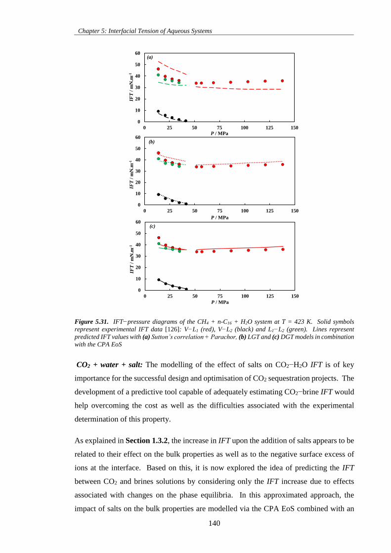
Chapter 5: Interfacial Tension of Aqueous Systems
140
Figure 5.31. IFT−pressure diagrams of the CH4 + n-C16 + H2O system at T = 423 K. Solid symbols
represent experimental IFT data [126]: V−L1 (red), V−L2 (black) and L1−L2 (green). Lines represent
predicted IFT values with (a) Sutton’s correlation + Parachor, (b) LGT and (c) DGT models in combination
with the CPA EoS
CO2 + water + salt: The modelling of the effect of salts on CO2−H2O IFT is of key
importance for the successful design and optimisation of CO2 sequestration projects. The
development of a predictive tool capable of adequately estimating CO2−brine IFT would
help overcoming the cost as well as the difficulties associated with the experimental
determination of this property.
As explained in Section 1.3.2, the increase in IFT upon the addition of salts appears to be
related to their effect on the bulk properties as well as to the negative surface excess of
ions at the interface. Based on this, it is now explored the idea of predicting the IFT
between CO2 and brines solutions by considering only the IFT increase due to effects
associated with changes on the phase equilibria. In this approximated approach, the
impact of salts on the bulk properties are modelled via the CPA EoS combined with an
0
10
20
30
40
50
60
0 25 50 75 100 125 150
IFT
/ m
N.m
-1
P / MPa
0
10
20
30
40
50
60
0 25 50 75 100 125 150
IFT
/ m
N.m
-1
P / MPa
0
10
20
30
40
50
60
0 25 50 75 100 125 150IF
T /
mN
.m-1
P / MPa
(a)
(b)
(c)
Chapter 5: Interfacial Tension of Aqueous Systems
141
electrolyte model and the accompanying IFT predicted via the density profiles of CO2
and H2O in a hypothetical salt-free system computed using the DGT. In other words, the
change in IFT is modelled by considering the salting-out effect and its influence on the
energy of both bulk phases and interface in a salt-free system. Such approach does not
account for the depletion of ions at the interface; however, initial results showed [103]
that this method lead to successful predictions of the IFT of CH4 + NaCl(aq) systems with
salt molalities up to 1.91 mol.kg-1. In this section, the model is extended to CO2 + brine
systems and the validity of such idea (approximation) is tested for higher salt molalities.
The impact of salts on the composition of the equilibrated phases has been considered by
using the method introduced by Aasberg-Petersen et al.[351] and extended to the CPA
EoS by Haghighi et al. [352]. Accordingly, the shift in the equilibrium conditions (i.e.,
V L
i i ) is evaluated by the addition of an electrostatic contribution to the fugacity
coefficient of components in the aqueous phase [351]:
ln ln lnEoS EL
i i i 5.5
where EoS
i is the fugacity coefficient of component i computed by the CPA EoS and EL
i
is the Debye-Hückel activity coefficient expressed as [351]:
1/2
3
2ln ( )EL is m
i
Ah Mf BI
B 5.6
where Mm is the salt-free mixture molecular weight, his is the adjustable interaction
coefficient between the salt and non-electrolytic components and, A and B are parameters
expressed as function of temperature and the dielectric constant of water. The parameters
A and B were transferred directly from the work of Aasberg-Petersen et al. [351] whereas
coefficients his, specifically optimised for CPA EoS, were used.
Water−salt interaction coefficients (hwater−salt) were taken equal to those of the work of
Haghighi et al. [87] and CO2−salt coefficients (hCO2−salt) were regressed here against
solubility data of CO2 in single salt systems for salt molalities up to 5 mol.kg-1. The
regressed coefficients, assumed to be function only of temperature, are listed in Table 5.8
for three salts (NaCl, KCl and CaCl2) along with the range of salinity and temperature
conditions of the experimental data used. The extension of calculations to mixed salt
solutions was performed by employing the approach suggested by Patwardhan and
Chapter 5: Interfacial Tension of Aqueous Systems
142
Kumar [353], and further tested by Tohidi-Kalorazi [354] and Haghighi [352].
Accordingly, the activity of a mixed salt solution (aw) can be evaluated by considering
the activity of the corresponding single salt solutions and calculated as follows [353]:
0
,log logsalt
w i w i
i
a y a 5.7
where 0
,w ia represents the activity of a single electrolyte solution of the same ionic strength
(I = 0.5 ∑j mj zj2, mi and zj correspond to the molality and charge of the jth ion, respectively)
as that of the mixed electrolyte solution and yi represents the ionic strength fraction of the
electrolyte i. The expression above does not include any empirical constants and thus,
the contribution of the electrostatic term for mixed salt solutions is obtained in a fully
predictive manner.
Table 5.8. Optimised CO2−salt interaction coefficients.
Salt Data Source Salt molality
msalt / mol.kg-1 T / K
2CO Salth
NaCl [324,355–357] 0.3 to 5.0 293 to 473 -3.6813×10⁻⁶ T2 + 2.8025 ×10⁻³ T - 0.4808
KCl [358,359] 1.0 to 4.5 313 to 433 -1.4933×10⁻⁶ T2 + 1.0512 ×10⁻³ T - 0.1624
CaCl2 [359,360] 0.3 to 5.0 309 to 424 -1.2369×10⁻⁶ T2 + 8.5643 ×10⁻⁴ T - 0.1155
As an example, a comparison between model estimates and experimental data for the
solubility of CO2 in NaCl and CaCl2 solutions is provided in Figures F.5 and F.6 in
APENDIX F. From these it can be observed that the CPA EoS + Electrolyte model can
successfully account for the decrease in CO2 solubility over a broad range of salt
molalities. Moreover, as can be seen in Figures F.7 through F.9 in APENDIX F, the use
of the regressed CO2−salt coefficients (Table 5.8) allowed a good prediction of the water
content in the CO2-rich phase of CO2 + brine systems as well as of CO2 solubility in
mixed salt solutions composed of NaCl, KCl and CaCl2. It is important to note that the
value of kij used for CO2−H2O throughout the present calculations was the same as that
calculated using the expression listed in Table 5.5.
Having shown the capabilities of the CPA EoS + Electrolyte model for describing the
phase equilibria of CO2 + brines systems, it is now possible to combine this model with
the DGT and to compute the density profiles of CO2 and H2O in a hypothetical salt-free
system and, in turn, the associated IFT. By keeping the binary interaction coefficient βij
Chapter 5: Interfacial Tension of Aqueous Systems
143
= 0.27 for CO2−H2O within the DGT framework (Table 5.6), the IFT of CO2 + brines
systems was predicted and the results compared to experimental data measured in the
present work as well as to that gathered from literature (Section 1.3.2). Results are plotted
in Figures 5.32 and 5.33 for selected isotherms.
As shown in Figures 5.32 and 5.33, the model can adequately predict the increase in IFT
due to the presence of salts such as NaCl, KCl and CaCl2 as well as their mixtures; good
agreement with experimental data measured here for CO2 + NaCl(aq) at T = 333 and 373
K and salt molalities up to 1.98 mol.kg-1 is observed. In addition, as substantiated
experimentally [113,115,119,129,130], predicted IFT values increase linearly with salt
molalities; as an example, results for CO2 + [0.864 NaCl + 0.136 KCl](aq) at T = 373 K
and selected isobars are plotted in Figure 5.34. However, for very concentrated brines,
and depending on the computed CO2−H2O IFT for the examined isotherm, the model
appears to overpredict severely the IFT of CO2 + brine systems, in particular for brines
containing CaCl2. It is important to note that IFT data measured by Aggelopoulos et al.
[129,130] for diluted brines containing CaCl2 persisted in being lower than CO2−H2O IFT
measured in the present work (Figures 5.32b and 5.33b), similar to what was described
previously for IFT data reported by others (Sections 1.3.2 and 5.3.3); yet, the differences
between predicted and experimentally determined IFT values at higher salt concentrations
cannot be attributed to the inconsistencies in the experiments alone. In turn, such
overprediction of IFT values may be most probably due to the strong salting-out effect of
CaCl2 compared to NaCl or KCl, which is intrinsically related to the ionic strength of the
brine. Based on these observations and on the modelling results for the examined brines,
it can be argued that such approximated treatment of the rise in IFT due the presence of
salts (via solubility change) appears to be adequate only for brines with low and medium
ionic strength (up to I = 2.7 mol.kg-1 or 0.9 mCaCl2) under the temperature conditions
examined.
The modelling results explained above are better interpreted by means of the Gibbs
adsorption equation. Accordingly, the change in CO2−brine IFT (dγ) can be related to
the chemical potentials (μ) of CO2 and ions as follows [361]:
2 2CO CO cation cation anion aniond at constant T 5.8
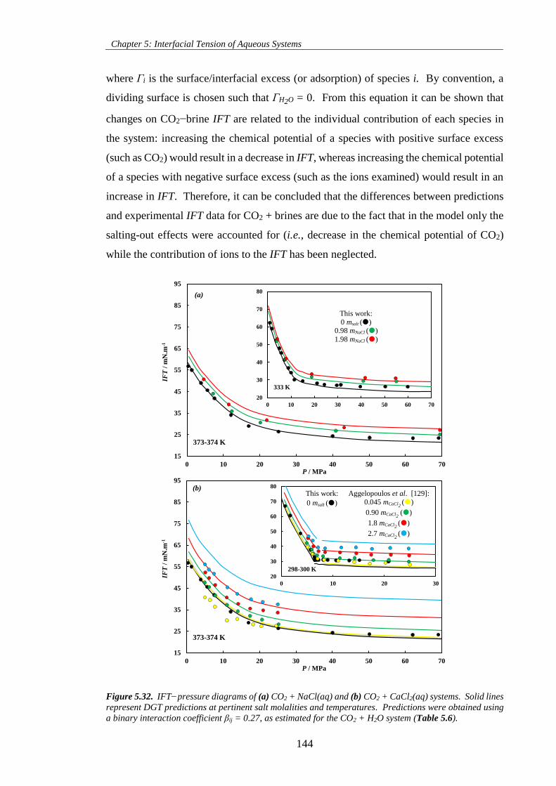
Chapter 5: Interfacial Tension of Aqueous Systems
144
where Γi is the surface/interfacial excess (or adsorption) of species i. By convention, a
dividing surface is chosen such that ΓH2O = 0. From this equation it can be shown that
changes on CO2−brine IFT are related to the individual contribution of each species in
the system: increasing the chemical potential of a species with positive surface excess
(such as CO2) would result in a decrease in IFT, whereas increasing the chemical potential
of a species with negative surface excess (such as the ions examined) would result in an
increase in IFT. Therefore, it can be concluded that the differences between predictions
and experimental IFT data for CO2 + brines are due to the fact that in the model only the
salting-out effects were accounted for (i.e., decrease in the chemical potential of CO2)
while the contribution of ions to the IFT has been neglected.
Figure 5.32. IFT−pressure diagrams of (a) CO2 + NaCl(aq) and (b) CO2 + CaCl2(aq) systems. Solid lines
represent DGT predictions at pertinent salt molalities and temperatures. Predictions were obtained using
a binary interaction coefficient βij = 0.27, as estimated for the CO2 + H2O system (Table 5.6).
15
25
35
45
55
65
75
85
95
0 10 20 30 40 50 60 70
IFT
/ m
N.m
-1
P / MPa
373-374 K
20
30
40
50
60
70
80
0 10 20 30 40 50 60 70
333 K
15
25
35
45
55
65
75
85
95
0 10 20 30 40 50 60 70
IFT
/ m
N.m
-1
P / MPa
373-374 K
20
30
40
50
60
70
80
0 10 20 30
298-300 K
(a)
(b)This work: Aggelopoulos et al. [129]:
0 msalt () 0.045 mCaCl2 ()
0.90 mCaCl2 ()
1.8 mCaCl2 ()
2.7 mCaCl2 ()
This work:
0 msalt () 0.98 mNaCl ()
1.98 mNaCl ()
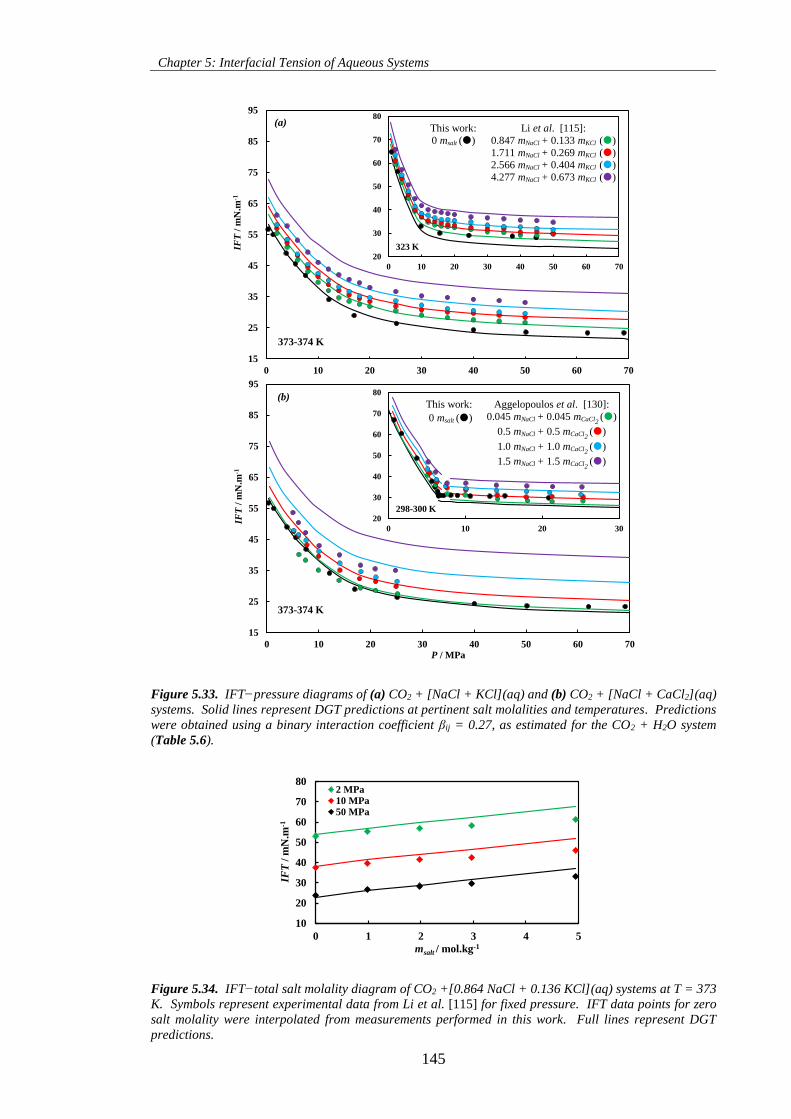
Chapter 5: Interfacial Tension of Aqueous Systems
145
Figure 5.33. IFT−pressure diagrams of (a) CO2 + [NaCl + KCl](aq) and (b) CO2 + [NaCl + CaCl2](aq)
systems. Solid lines represent DGT predictions at pertinent salt molalities and temperatures. Predictions
were obtained using a binary interaction coefficient βij = 0.27, as estimated for the CO2 + H2O system
(Table 5.6).
Figure 5.34. IFT−total salt molality diagram of CO2 +[0.864 NaCl + 0.136 KCl](aq) systems at T = 373
K. Symbols represent experimental data from Li et al. [115] for fixed pressure. IFT data points for zero
salt molality were interpolated from measurements performed in this work. Full lines represent DGT
predictions.
15
25
35
45
55
65
75
85
95
0 10 20 30 40 50 60 70
IFT
/ m
N.m
-1
P / MPa
373-374 K
20
30
40
50
60
70
80
0 10 20 30 40 50 60 70
323 K
15
25
35
45
55
65
75
85
95
0 10 20 30 40 50 60 70
IFT
/ m
N.m
-1
P / MPa
373-374 K
20
30
40
50
60
70
80
0 10 20 30
298-300 K
(b)
(a)
10
20
30
40
50
60
70
80
0 1 2 3 4 5
IFT
/ m
N.m
-1
msalt / mol.kg-1
2 MPa10 MPa50 MPa
This work: Aggelopoulos et al. [130]:
0 msalt () 0.045 mNaCl + 0.045 mCaCl2 ()
0.5 mNaCl + 0.5 mCaCl2 ()
1.0 mNaCl + 1.0 mCaCl2 ()
1.5 mNaCl + 1.5 mCaCl2 ()
This work: Li et al. [115]:
0 msalt () 0.847 mNaCl + 0.133 mKCl ()
1.711 mNaCl + 0.269 mKCl ()
2.566 mNaCl + 0.404 mKCl ()
4.277 mNaCl + 0.673 mKCl ()
Chapter 5: Interfacial Tension of Aqueous Systems
146
5.5 Microstructure of Interfaces
As done in Section 4.5 for the hydrocarbon systems, the density profiles of the aqueous
systems computed using the DGT are analysed in the present section and the impact of
the microstructure of the interface on the IFT is discussed.
First, the effect of using a binary interaction coefficient βij ≠ 0 is described. As an
example, the density profiles computed using different values for βij are plotted in Figures
5.35, 5.36 and 5.37 for the systems CO2 + H2O, CH4 + H2O and n-C10 + H2O at selected
temperatures and pressures. The density profiles of the CO2 + H2O (Figure 5.35) and
CH4 + H2O (Figure 5.36) systems show a local enrichment of the interface in CO2 and
CH4 molecules, as noticed by the appearance of adsorption peaks in the density profiles
of CO2 and CH4, whereas the density profile of water follows the usual tanh shape,
increasing monotonically from the CO2/CH4-rich phase to the water-rich phase. It can
also be observed from these figures that the use of βij = 0 leads to the computation of very
sharp peaks (infinitely steep) at the interface; interfacial tensions associated with these
profiles are those plotted in Figure 5.22, where a kink in the IFT−pressure diagram was
observed. The appearance of such steep gradients creates some numerical convergence
problems which are rather difficult to overcome [250]. A simple way of avoiding these
problems is by using a value for βij ≠ 0. For the CO2 + H2O and CH4 + H2O systems, the
use of positive and increasing values of βij results in a reduction of the maximum
concentration of the components with interfacial activity which, in turn, leads to a better
agreement between the accompanying IFT and that experimentally determined, as
previously described.
Density profiles of the n-C10 + H2O system computed using βij = 0.02 suggest some degree
of adsorption of n-C10 in the interface, as depicted in the insert of Figure 5.37; however,
the use of the optimal value for IFT estimation (βij = 0.44) leads to the computation of
less steep and broader density profiles for n-C10 and H2O and apparently reduces the
amount of n-C10 in the interface. The effect of broadening the interface would lead to a
decrease in IFT, whereas the removal of n-C10 molecules from the interface would result
in increase in IFT. Since better agreement with experimental IFT data was achieved using
higher values of βij, the withdrawal of n-C10 molecules from the interface appears to have
a stronger influence on the computed IFT values at the thermodynamic conditions
examined.
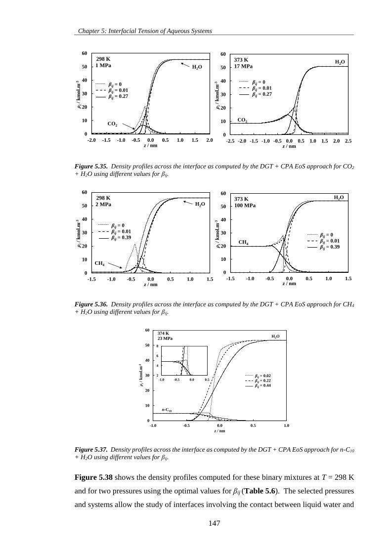
Chapter 5: Interfacial Tension of Aqueous Systems
147
Figure 5.35. Density profiles across the interface as computed by the DGT + CPA EoS approach for CO2
+ H2O using different values for βij.
Figure 5.36. Density profiles across the interface as computed by the DGT + CPA EoS approach for CH4
+ H2O using different values for βij.
Figure 5.37. Density profiles across the interface as computed by the DGT + CPA EoS approach for n-C10
+ H2O using different values for βij.
Figure 5.38 shows the density profiles computed for these binary mixtures at T = 298 K
and for two pressures using the optimal values for βij (Table 5.6). The selected pressures
and systems allow the study of interfaces involving the contact between liquid water and
0
10
20
30
40
50
60
-2.0 -1.5 -1.0 -0.5 0.0 0.5 1.0 1.5 2.0
ρi/
km
ol.
m-3
z / nm
298 K
1 MPa
Series2
Series4
Series5
H2O
βij = 0
βij = 0.01
βij = 0.27
CO2
0
10
20
30
40
50
60
-2.5 -2.0 -1.5 -1.0 -0.5 0.0 0.5 1.0 1.5 2.0 2.5
ρi/
km
ol.
m-3
z / nm
373 K
17 MPa
Series2
Series1
Series6
βij = 0
βij = 0.01
βij = 0.27
H2O
CO2
0
10
20
30
40
50
60
-1.5 -1.0 -0.5 0.0 0.5 1.0 1.5
ρi/
km
ol.
m-3
z / nm
298 K
2 MPa
Series3
Series1
Series6
βij = 0
βij = 0.01
βij = 0.39
CH4
H2O
0
10
20
30
40
50
60
-1.5 -1.0 -0.5 0.0 0.5 1.0 1.5
ρi/
km
ol.
m-3
z / nm
373 K
100 MPa
Series2
Series4
Series6
βij = 0
βij = 0.01
βij = 0.39CH4
H2O
0
10
20
30
40
50
60
-1.0 -0.5 0.0 0.5 1.0
ρi/
km
ol.
m-3
z / nm
374 K
23 MPa
Series4
Series2
Series5
n-C10
H2O
βij = 0.02
βij = 0.22
βij = 0.44
2
4
6
8
-1.0 -0.5 0.0 0.5
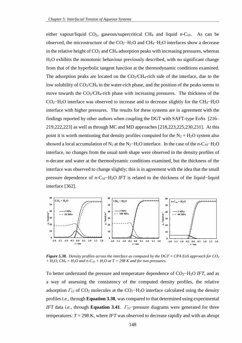
Chapter 5: Interfacial Tension of Aqueous Systems
148
either vapour/liquid CO2, gaseous/supercritical CH4 and liquid n-C10. As can be
observed, the microstructure of the CO2−H2O and CH4−H2O interfaces show a decrease
in the relative height of CO2 and CH4 adsorption peaks with increasing pressures, whereas
H2O exhibits the monotonic behaviour previously described, with no significant change
from that of the hyperbolic tangent function at the thermodynamic conditions examined.
The adsorption peaks are located on the CO2/CH4-rich side of the interface, due to the
low solubility of CO2/CH4 in the water-rich phase, and the position of the peaks seems to
move towards the CO2/CH4-rich phase with increasing pressures. The thickness of the
CO2−H2O interface was observed to increase and to decrease slightly for the CH4−H2O
interface with higher pressures. The results for these systems are in agreement with the
findings reported by other authors when coupling the DGT with SAFT-type EoSs [216–
219,222,223] as well as through MC and MD approaches [218,223,225,230,231]. At this
point it is worth mentioning that density profiles computed for the N2 + H2O system also
showed a local accumulation of N2 at the N2−H2O interface. In the case of the n-C10−H2O
interface, no changes from the usual tanh shape were observed in the density profiles of
n-decane and water at the thermodynamic conditions examined, but the thickness of the
interface was observed to change slightly; this is in agreement with the idea that the small
pressure dependence of n-C10−H2O IFT is related to the thickness of the liquid−liquid
interface [362].
Figure 5.38. Density profiles across the interface as computed by the DGT + CPA EoS approach for CO2
+ H2O, CH4 + H2O and n-C10 + H2O at T = 298 K and for two pressures.
To better understand the pressure and temperature dependence of CO2−H2O IFT, and as
a way of assessing the consistency of the computed density profiles, the relative
adsorption Γ12 of CO2 molecules at the CO2−H2O interface calculated using the density
profiles i.e., through Equation 3.38, was compared to that determined using experimental
IFT data i.e., through Equation 3.41. Γ12−pressure diagrams were generated for three
temperatures: T = 298 K, where IFT was observed to decrease rapidly and with an abrupt
0
10
20
30
40
50
60
-2.0 -1.5 -1.0 -0.5 0.0 0.5 1.0 1.5 2.0
ρi/
km
ol.
m-3
z / nm
CO2 + H2O
2 MPa
10 MPa
0
10
20
30
40
50
60
-2.0 -1.5 -1.0 -0.5 0.0 0.5 1.0 1.5 2.0
ρi/
km
ol.
m-3
z / nm
CH4 + H2O
2 MPa
100 MPa
0
10
20
30
40
50
60
-2.0 -1.5 -1.0 -0.5 0.0 0.5 1.0 1.5 2.0
ρi/
km
ol.
m-3
z / nm
n-C10 + H2O
1 MPa
40 MPa
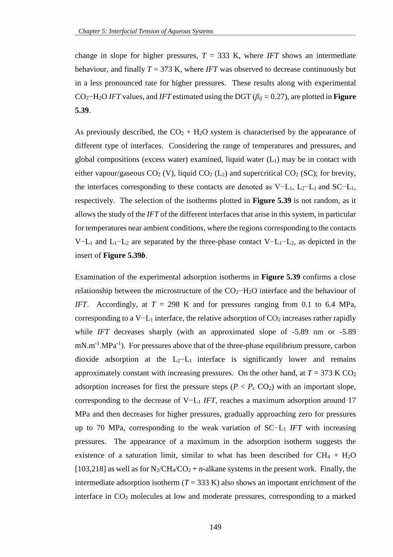
Chapter 5: Interfacial Tension of Aqueous Systems
149
change in slope for higher pressures, T = 333 K, where IFT shows an intermediate
behaviour, and finally T = 373 K, where IFT was observed to decrease continuously but
in a less pronounced rate for higher pressures. These results along with experimental
CO2−H2O IFT values, and IFT estimated using the DGT (βij = 0.27), are plotted in Figure
5.39.
As previously described, the CO2 + H2O system is characterised by the appearance of
different type of interfaces. Considering the range of temperatures and pressures, and
global compositions (excess water) examined, liquid water (L1) may be in contact with
either vapour/gaseous CO2 (V), liquid CO2 (L2) and supercritical CO2 (SC); for brevity,
the interfaces corresponding to these contacts are denoted as V−L1, L2−L1 and SC−L1,
respectively. The selection of the isotherms plotted in Figure 5.39 is not random, as it
allows the study of the IFT of the different interfaces that arise in this system, in particular
for temperatures near ambient conditions, where the regions corresponding to the contacts
V−L1 and L1−L2 are separated by the three-phase contact V−L1−L2, as depicted in the
insert of Figure 5.39b.
Examination of the experimental adsorption isotherms in Figure 5.39 confirms a close
relationship between the microstructure of the CO2−H2O interface and the behaviour of
IFT. Accordingly, at T = 298 K and for pressures ranging from 0.1 to 6.4 MPa,
corresponding to a V−L1 interface, the relative adsorption of CO2 increases rather rapidly
while IFT decreases sharply (with an approximated slope of -5.89 nm or -5.89
mN.m-1.MPa-1). For pressures above that of the three-phase equilibrium pressure, carbon
dioxide adsorption at the L2−L1 interface is significantly lower and remains
approximately constant with increasing pressures. On the other hand, at T = 373 K CO2
adsorption increases for first the pressure steps (P < Pc CO2) with an important slope,
corresponding to the decrease of V−L1 IFT, reaches a maximum adsorption around 17
MPa and then decreases for higher pressures, gradually approaching zero for pressures
up to 70 MPa, corresponding to the weak variation of SC−L1 IFT with increasing
pressures. The appearance of a maximum in the adsorption isotherm suggests the
existence of a saturation limit, similar to what has been described for CH4 + H2O
[103,218] as well as for N2/CH4/CO2 + n-alkane systems in the present work. Finally, the
intermediate adsorption isotherm (T = 333 K) also shows an important enrichment of the
interface in CO2 molecules at low and moderate pressures, corresponding to a marked
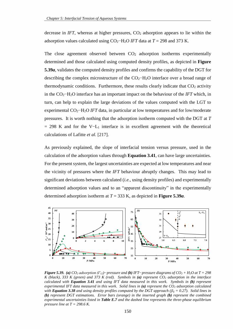
Chapter 5: Interfacial Tension of Aqueous Systems
150
decrease in IFT, whereas at higher pressures, CO2 adsorption appears to lie within the
adsorption values calculated using CO2−H2O IFT data at T = 298 and 373 K.
The close agreement observed between CO2 adsorption isotherms experimentally
determined and those calculated using computed density profiles, as depicted in Figure
5.39a, validates the computed density profiles and confirms the capability of the DGT for
describing the complex microstructure of the CO2−H2O interface over a broad range of
thermodynamic conditions. Furthermore, these results clearly indicate that CO2 activity
in the CO2−H2O interface has an important impact on the behaviour of the IFT which, in
turn, can help to explain the large deviations of the values computed with the LGT to
experimental CO2−H2O IFT data, in particular at low temperatures and for low/moderate
pressures. It is worth nothing that the adsorption isotherm computed with the DGT at T
= 298 K and for the V−L1 interface is in excellent agreement with the theoretical
calculations of Lafitte et al. [217].
As previously explained, the slope of interfacial tension versus pressure, used in the
calculation of the adsorption values through Equation 3.41, can have large uncertainties.
For the present system, the largest uncertainties are expected at low temperatures and near
the vicinity of pressures where the IFT behaviour abruptly changes. This may lead to
significant deviations between calculated (i.e., using density profiles) and experimentally
determined adsorption values and to an “apparent discontinuity” in the experimentally
determined adsorption isotherm at T = 333 K, as depicted in Figure 5.39a.
Figure 5.39. (a) CO2 adsorption (Γ12)−pressure and (b) IFT−pressure diagrams of CO2 + H2O at T = 298
K (black), 333 K (green) and 373 K (red). Symbols in (a) represent CO2 adsorption in the interface
calculated with Equation 3.41 and using IFT data measured in this work. Symbols in (b) represent
experimental IFT data measured in this work. Solid lines in (a) represent the CO2 adsorption calculated
with Equation 3.38 and using density profiles computed by the DGT approach (βij = 0.27). Solid lines in
(b) represent DGT estimations. Error bars (orange) in the inserted graph (b) represent the combined
experimental uncertainties listed in Table E.7 and the dashed line represents the three-phase equilibrium
pressure line at T = 298.6 K.
0
5
10
15
20
25
30
35
40
45
0 10 20 30 40 50 60 70
Γ1
2/
10
-6m
ol.
m-2
P /MPa
(a)
15
25
35
45
55
65
75
0 10 20 30 40 50 60 70
IFT
/ m
N.m
-1
P /MPa
0
10
20
30
40
0 2 4 6 8 10
27
29
31
33
35
5.8 6.3 6.8 7.3 7.8
L2−L1
V−
L1−
L2
V−L1
(b)
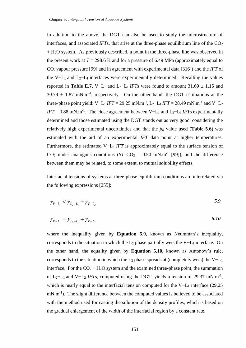
Chapter 5: Interfacial Tension of Aqueous Systems
151
In addition to the above, the DGT can also be used to study the microstructure of
interfaces, and associated IFTs, that arise at the three-phase equilibrium line of the CO2
+ H2O system. As previously described, a point in the three-phase line was observed in
the present work at T = 298.6 K and for a pressure of 6.49 MPa (approximately equal to
CO2 vapour pressure [99] and in agreement with experimental data [316]) and the IFT of
the V−L1 and L2−L1 interfaces were experimentally determined. Recalling the values
reported in Table E.7, V−L1 and L2−L1 IFTs were found to amount 31.69 ± 1.15 and
30.79 ± 1.87 mN.m-1, respectively. On the other hand, the DGT estimations at the
three-phase point yield: V−L1 IFT = 29.25 mN.m-1, L2−L1 IFT = 28.49 mN.m-1 and V−L2
IFT = 0.88 mN.m-1. The close agreement between V−L1 and L2−L1 IFTs experimentally
determined and those estimated using the DGT stands out as very good, considering the
relatively high experimental uncertainties and that the βij value used (Table 5.6) was
estimated with the aid of an experimental IFT data point at higher temperatures.
Furthermore, the estimated V−L2 IFT is approximately equal to the surface tension of
CO2 under analogous conditions (ST CO2 = 0.50 mN.m-1 [99]), and the difference
between them may be related, to some extent, to mutual solubility effects.
Interfacial tensions of systems at three-phase equilibrium conditions are interrelated via
the following expressions [255]:
1 2 1 2V L L L V L 5.9
1 2 1 2V L L L V L 5.10
where the inequality given by Equation 5.9, known as Neumman’s inequality,
corresponds to the situation in which the L2 phase partially wets the V−L1 interface. On
the other hand, the equality given by Equation 5.10, known as Antonow’s rule,
corresponds to the situation in which the L2 phase spreads at (completely wets) the V−L1
interface. For the CO2 + H2O system and the examined three-phase point, the summation
of L2−L1 and V−L2 IFTs, computed using the DGT, yields a tension of 29.37 mN.m-1,
which is nearly equal to the interfacial tension computed for the V−L1 interface (29.25
mN.m-1). The slight difference between the computed values is believed to be associated
with the method used for casting the solution of the density profiles, which is based on
the gradual enlargement of the width of the interfacial region by a constant rate.
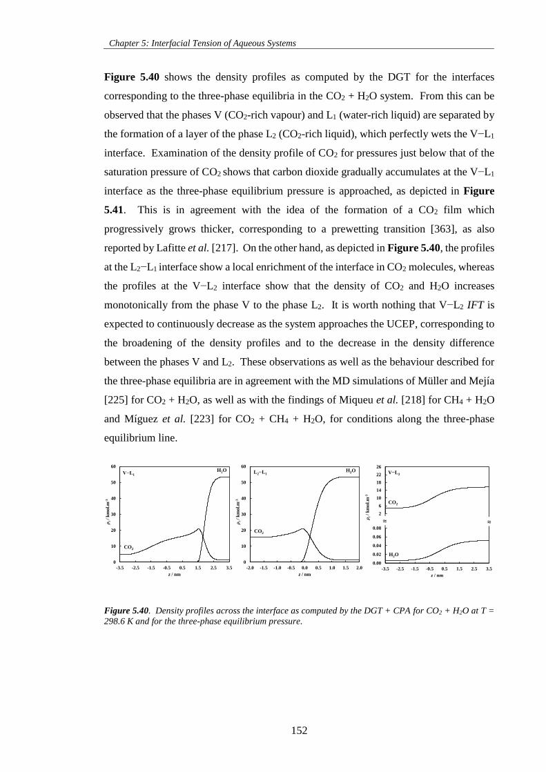
Chapter 5: Interfacial Tension of Aqueous Systems
152
Figure 5.40 shows the density profiles as computed by the DGT for the interfaces
corresponding to the three-phase equilibria in the CO2 + H2O system. From this can be
observed that the phases V (CO2-rich vapour) and L1 (water-rich liquid) are separated by
the formation of a layer of the phase L2 (CO2-rich liquid), which perfectly wets the V−L1
interface. Examination of the density profile of CO2 for pressures just below that of the
saturation pressure of CO2 shows that carbon dioxide gradually accumulates at the V−L1
interface as the three-phase equilibrium pressure is approached, as depicted in Figure
5.41. This is in agreement with the idea of the formation of a CO2 film which
progressively grows thicker, corresponding to a prewetting transition [363], as also
reported by Lafitte et al. [217]. On the other hand, as depicted in Figure 5.40, the profiles
at the L2−L1 interface show a local enrichment of the interface in CO2 molecules, whereas
the profiles at the V−L2 interface show that the density of CO2 and H2O increases
monotonically from the phase V to the phase L2. It is worth nothing that V−L2 IFT is
expected to continuously decrease as the system approaches the UCEP, corresponding to
the broadening of the density profiles and to the decrease in the density difference
between the phases V and L2. These observations as well as the behaviour described for
the three-phase equilibria are in agreement with the MD simulations of Müller and Mejía
[225] for CO2 + H2O, as well as with the findings of Miqueu et al. [218] for CH4 + H2O
and Míguez et al. [223] for CO2 + CH4 + H2O, for conditions along the three-phase
equilibrium line.
Figure 5.40. Density profiles across the interface as computed by the DGT + CPA for CO2 + H2O at T =
298.6 K and for the three-phase equilibrium pressure.
0
10
20
30
40
50
60
-2.0 -1.5 -1.0 -0.5 0.0 0.5 1.0 1.5 2.0
ρi/
km
ol.
m-3
z / nm
L2−L1
0
10
20
30
40
50
60
-3.5 -2.5 -1.5 -0.5 0.5 1.5 2.5 3.5
ρi/
km
ol.
m-3
z / nm
V−L1
2
6
10
14
18
22
26
ρi/
km
ol.
m-3
V−L2
0.00
0.02
0.04
0.06
0.08
-3.5 -2.5 -1.5 -0.5 0.5 1.5 2.5 3.5
z / nm
≈ ≈
CO2
H2O H2O
H2O
CO2
CO2
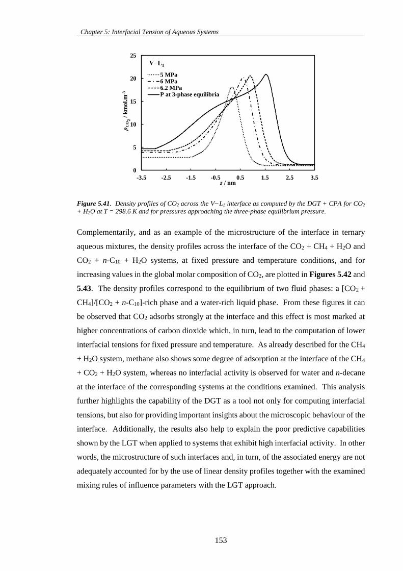
Chapter 5: Interfacial Tension of Aqueous Systems
153
Figure 5.41. Density profiles of CO2 across the V−L1 interface as computed by the DGT + CPA for CO2
+ H2O at T = 298.6 K and for pressures approaching the three-phase equilibrium pressure.
Complementarily, and as an example of the microstructure of the interface in ternary
aqueous mixtures, the density profiles across the interface of the CO2 + CH4 + H2O and
CO2 + n-C10 + H2O systems, at fixed pressure and temperature conditions, and for
increasing values in the global molar composition of CO2, are plotted in Figures 5.42 and
5.43. The density profiles correspond to the equilibrium of two fluid phases: a [CO2 +
CH4]/[CO2 + n-C10]-rich phase and a water-rich liquid phase. From these figures it can
be observed that CO2 adsorbs strongly at the interface and this effect is most marked at
higher concentrations of carbon dioxide which, in turn, lead to the computation of lower
interfacial tensions for fixed pressure and temperature. As already described for the CH4
+ H2O system, methane also shows some degree of adsorption at the interface of the CH4
+ CO2 + H2O system, whereas no interfacial activity is observed for water and n-decane
at the interface of the corresponding systems at the conditions examined. This analysis
further highlights the capability of the DGT as a tool not only for computing interfacial
tensions, but also for providing important insights about the microscopic behaviour of the
interface. Additionally, the results also help to explain the poor predictive capabilities
shown by the LGT when applied to systems that exhibit high interfacial activity. In other
words, the microstructure of such interfaces and, in turn, of the associated energy are not
adequately accounted for by the use of linear density profiles together with the examined
mixing rules of influence parameters with the LGT approach.
0
5
10
15
20
25
-3.5 -2.5 -1.5 -0.5 0.5 1.5 2.5 3.5
ρC
O2
/ k
mo
l.m
-3
z / nm
V−L1
5 MPa6 MPa6.2 MPaP at 3-phase equilibria
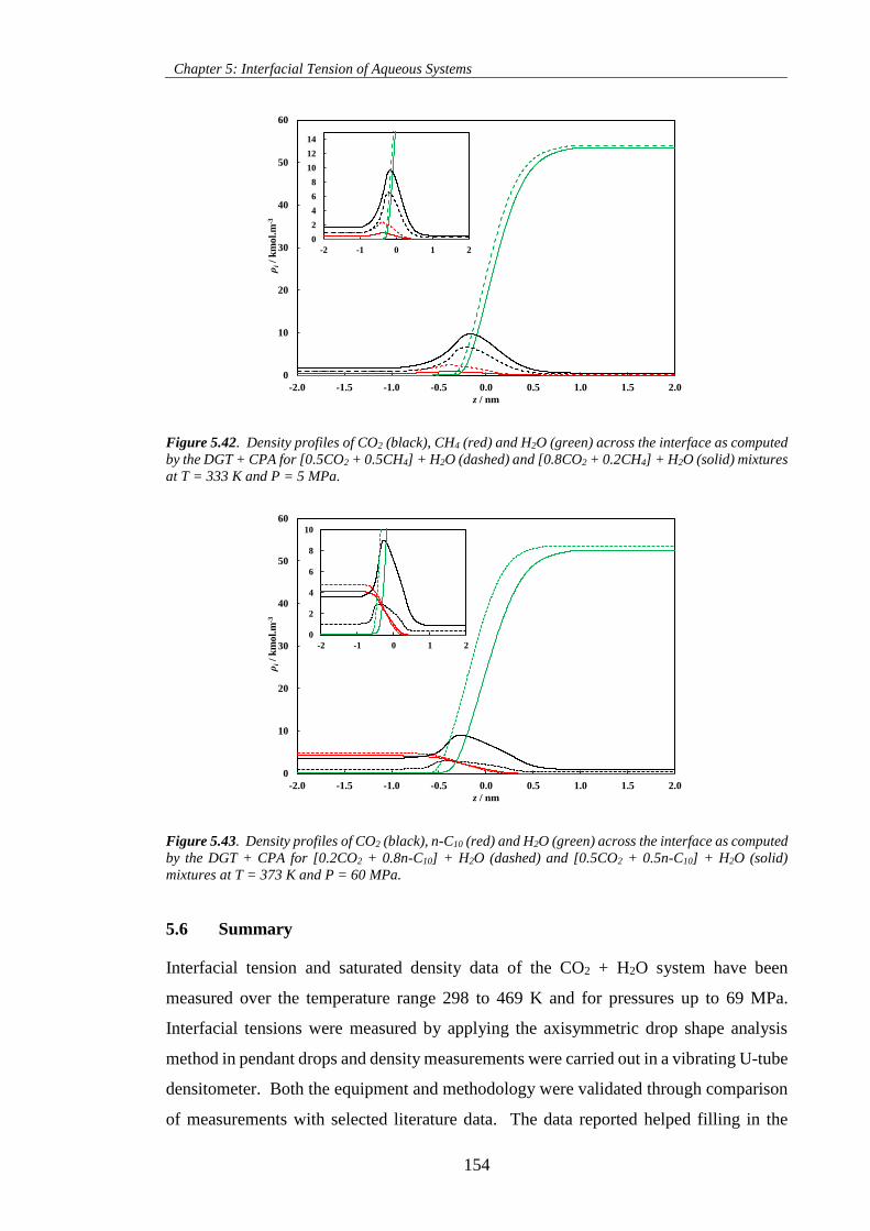
Chapter 5: Interfacial Tension of Aqueous Systems
154
Figure 5.42. Density profiles of CO2 (black), CH4 (red) and H2O (green) across the interface as computed
by the DGT + CPA for [0.5CO2 + 0.5CH4] + H2O (dashed) and [0.8CO2 + 0.2CH4] + H2O (solid) mixtures
at T = 333 K and P = 5 MPa.
Figure 5.43. Density profiles of CO2 (black), n-C10 (red) and H2O (green) across the interface as computed
by the DGT + CPA for [0.2CO2 + 0.8n-C10] + H2O (dashed) and [0.5CO2 + 0.5n-C10] + H2O (solid)
mixtures at T = 373 K and P = 60 MPa.
5.6 Summary
Interfacial tension and saturated density data of the CO2 + H2O system have been
measured over the temperature range 298 to 469 K and for pressures up to 69 MPa.
Interfacial tensions were measured by applying the axisymmetric drop shape analysis
method in pendant drops and density measurements were carried out in a vibrating U-tube
densitometer. Both the equipment and methodology were validated through comparison
of measurements with selected literature data. The data reported helped filling in the
0
10
20
30
40
50
60
-2.0 -1.5 -1.0 -0.5 0.0 0.5 1.0 1.5 2.0
ρi/
km
ol.
m-3
z / nm
0
2
4
6
8
10
12
14
-2 -1 0 1 2
0
10
20
30
40
50
60
-2.0 -1.5 -1.0 -0.5 0.0 0.5 1.0 1.5 2.0
ρi/
km
ol.
m-3
z / nm
0
2
4
6
8
10
-2 -1 0 1 2
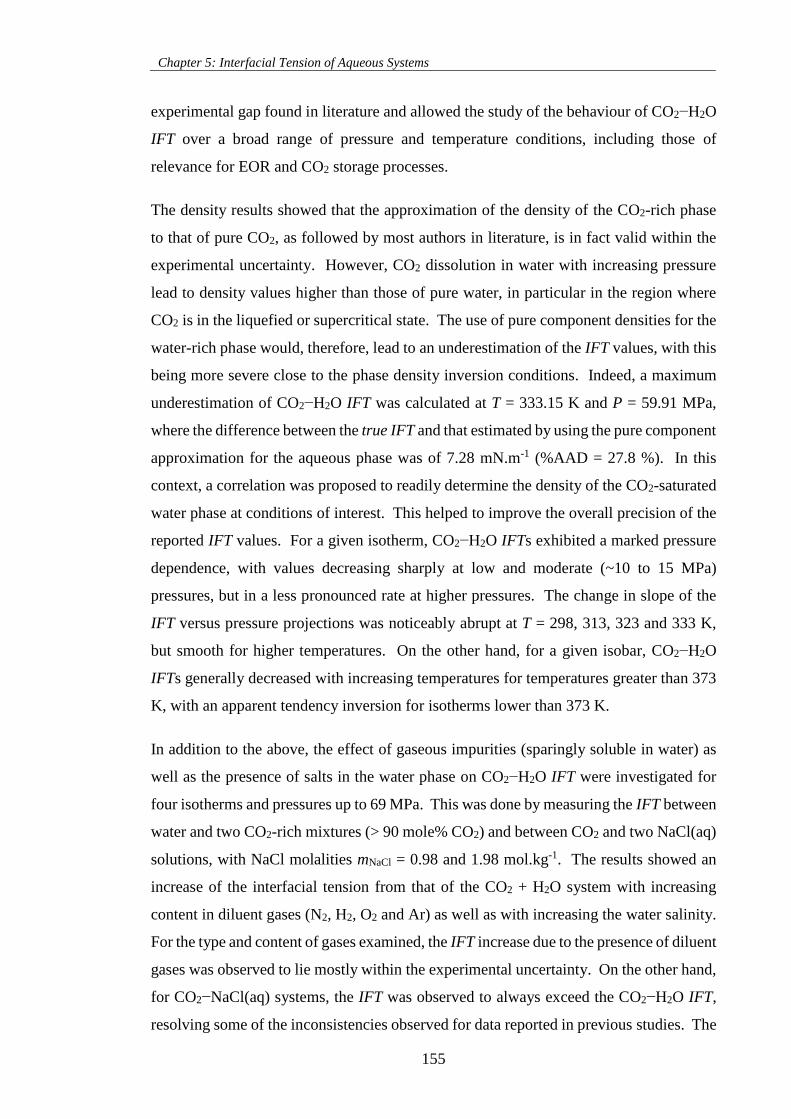
Chapter 5: Interfacial Tension of Aqueous Systems
155
experimental gap found in literature and allowed the study of the behaviour of CO2−H2O
IFT over a broad range of pressure and temperature conditions, including those of
relevance for EOR and CO2 storage processes.
The density results showed that the approximation of the density of the CO2-rich phase
to that of pure CO2, as followed by most authors in literature, is in fact valid within the
experimental uncertainty. However, CO2 dissolution in water with increasing pressure
lead to density values higher than those of pure water, in particular in the region where
CO2 is in the liquefied or supercritical state. The use of pure component densities for the
water-rich phase would, therefore, lead to an underestimation of the IFT values, with this
being more severe close to the phase density inversion conditions. Indeed, a maximum
underestimation of CO2−H2O IFT was calculated at T = 333.15 K and P = 59.91 MPa,
where the difference between the true IFT and that estimated by using the pure component
approximation for the aqueous phase was of 7.28 mN.m-1 (%AAD = 27.8 %). In this
context, a correlation was proposed to readily determine the density of the CO2-saturated
water phase at conditions of interest. This helped to improve the overall precision of the
reported IFT values. For a given isotherm, CO2−H2O IFTs exhibited a marked pressure
dependence, with values decreasing sharply at low and moderate (~10 to 15 MPa)
pressures, but in a less pronounced rate at higher pressures. The change in slope of the
IFT versus pressure projections was noticeably abrupt at T = 298, 313, 323 and 333 K,
but smooth for higher temperatures. On the other hand, for a given isobar, CO2−H2O
IFTs generally decreased with increasing temperatures for temperatures greater than 373
K, with an apparent tendency inversion for isotherms lower than 373 K.
In addition to the above, the effect of gaseous impurities (sparingly soluble in water) as
well as the presence of salts in the water phase on CO2−H2O IFT were investigated for
four isotherms and pressures up to 69 MPa. This was done by measuring the IFT between
water and two CO2-rich mixtures (> 90 mole% CO2) and between CO2 and two NaCl(aq)
solutions, with NaCl molalities mNaCl = 0.98 and 1.98 mol.kg-1. The results showed an
increase of the interfacial tension from that of the CO2 + H2O system with increasing
content in diluent gases (N2, H2, O2 and Ar) as well as with increasing the water salinity.
For the type and content of gases examined, the IFT increase due to the presence of diluent
gases was observed to lie mostly within the experimental uncertainty. On the other hand,
for CO2−NaCl(aq) systems, the IFT was observed to always exceed the CO2−H2O IFT,
resolving some of the inconsistencies observed for data reported in previous studies. The
Chapter 5: Interfacial Tension of Aqueous Systems
156
increase in interfacial tension averaged an amount between 1.42 and 2.01 mN.m-1 for
mNaCl = 0.98 mol.kg-1 and between 2.67 and 3.73 mN.m-1 for mNaCl = 1.98 mol.kg-1. This
corresponds to an average relative increase from CO2−H2O IFT between 4.4 and 13.2%,
over the range of pressures, temperatures and salt molalities examined here.
A brief discussion of the impact of CO2−H2O IFT on the capillary-sealing efficiency of
caprocks was presented. The results suggest the existence of an optimal caprock depth
for the storage of CO2 in reservoirs located onshore, whereas for reservoirs located
offshore, CO2 trapping potential appeared to decrease progressively with increasing
caprock depth. Nonetheless, by comparing these two scenarios, it was evident that
caprocks in offshore fields can potentially trap significantly higher quantities of CO2. In
addition to this, the analysis of the impact of gaseous sparingly soluble impurities and
water salinity indicated that they would have a positive effect on the capillary-sealing
efficiency of caprocks.
The interfacial tension of binary and multicomponent aqueous systems measured in the
present work as well as reported by others in literature were compared to theoretical
calculations obtained with the DGT in combination with the CPA EoS. Comparison to
calculations with the LGT approach and empirical methods, such as the Parachor and
Sutton’s correlation, was also performed. The systems investigated included conditions
at which one aqueous phase was simultaneously in contact with one or two fluid phases.
The results showed that by using constant influence parameters and a single, temperature
independent, binary interaction coefficient adjusted to one IFT data point at moderate
conditions, the DGT was capable of describing the IFT of two- and three-phase aqueous
systems over a broad range of pressure and temperature conditions, with deviations to
experimental data lower than that obtained using other IFT models. The DGT performed
significantly well when describing the complex behaviour of the CO2 + H2O system,
namely the high pressure dependence of the interfacial tension. Moreover, the impact of
salts was also adequately replicated, up to a certain limit of ionic strength, by modelling
the salting-out effect and computing the IFT associated with the density profiles in a
hypothetical salt-free system. Overall, the DGT in combination with the CPA EoS was
capable of accounting for the IFT variations in aqueous systems of relevance for EOR
and CO2 storage processes due to changes in composition, temperature and pressure.

Chapter 5: Interfacial Tension of Aqueous Systems
157
Further to the above, the density profiles computed with the DGT were examined and the
impact of the microstructure of the interface on the IFT was discussed. The use of βij ≠ 0
helped to circumvent the numerical difficulties encountered in the solution of the
equations governing the density profiles of aqueous systems; the appearance of infinitely
steep density profiles was pointed out as a possible cause. The use of the optimal values
of βij for interfacial tension estimations showed a tendency of CO2, CH4 and N2 molecules
to accumulate at the interface of aqueous systems, as reflected by the appearance of
adsorption peaks in the density profiles. In the case of the CO2 + H2O system, a good
agreement between the Gibbs adsorption isotherms computed using the density profiles
and those computed using experimental CO2−H2O IFT was found. This validates to some
extent the computed density profiles and confirms the adequacy of the DGT for describing
the complex microstructure of aqueous interfaces. Particular attention was given to the
CO2−H2O interface near the vicinity of the three-phase equilibrium line, with density
profiles showing the formation of a thin CO2 film as the saturation pressure of CO2 was
approached. This behaviour was found to be in agreement with the findings reported by
others in previous studies available in literature. Furthermore, density profiles computed
for the ternary systems CO2 + n-C10 + H2O and CO2 + CH4 + H2O showed an increasing
enrichment of the fluid−liquid interface in CO2 molecules by increasing the global content
in CO2, readily linking the reduction of interfacial tension to the interfacial activity of
CO2. Together, these results also helped to explain the poor modelling results obtained
with the LGT for aqueous interfaces. Accordingly, it appears that the energy of such
interfaces and, in turn, the IFT are not adequately described by the use of linear density
profiles together with the mixing rules of influence parameters examined within the
framework of the LGT.
158
CHAPTER 6 – CONCLUSIONS AND RECOMMENDATIONS FOR
FUTURE WORK
6.1 Introduction
In this thesis the interfacial tension of reservoir fluids in the context of enhanced oil
recovery processes and CO2 storage in underground formations has been investigated.
The investigations covered both experimental and modelling aspects of the interfacial
tension of fluid−liquid interfaces in hydrocarbon and aqueous systems over a broad range
of conditions (from ambient up to 473 K and 300 MPa). The examined systems
comprised binary and multicomponent synthetic mixtures including n-alkanes, water,
salts and gases, as well as one real petroleum fluid. Though most of the systems studied
here were simple in terms of the number of components, they are not devoid of
complexities as obtainable in real reservoirs. Interfacial tensions were observed to span
from near complete miscibility (low IFT values) to immiscible (high IFT values) two- and
three-phase equilibria conditions. Moreover, as well as complementing and extending
the range of experimental data sets available in literature, the data measured in this thesis
(and by others) were used for testing the capability of theoretical tools for replicating the
IFT variations in reservoir fluids due to changes in composition, temperature and
pressure. More specific details on the experimental and modelling achievements and
results of this thesis are briefly outlined below. Recommendations for future
investigations are also described in this chapter.
6.2 Experimental Investigation
Two new HPHT apparatus were constructed and used to measure the interfacial tension
between fluid phases. One was based on the Differential Capillary Rise method and was
suitable for measuring the interfacial tension of hydrocarbon systems, where low tension
values can be attained at sufficiently high pressure and temperature conditions. The other,
used for aqueous systems, was based on the Pendant Drop method and the axisymmetric
drop shape analysis technique. The measurement of true IFT values requires the accurate
estimation of the density of the phases in contact. Therefore, saturated phase density data
were measured using a vibrating U-tube densitometer and the generated densities used
directly or as correlating data for the experimental determination of IFT values.
Chapter 6: Conclusions and Recommendations for Future Work
159
The interfacial tension and saturated density of gas + oil systems were measured for three
binary mixtures CH4 + n-decane, CO2 + n-decane and N2 + n-decane as well as for three
multicomponent synthetic mixtures composed of CH4, CO2, N2 and n-alkanes, in a total
of up to 9 components. These properties were investigated in the binary mixtures for four
isotherms 313, 344, 393 and 443 K and pressures up to 69 MPa or near the critical point
of each mixture. Good agreement with literature data at pertinent conditions was
observed, validating both the equipment and methodology as well as extending the range
of conditions available from previous studies. The multicomponent mixtures were
investigated at a representative reservoir temperature of 393 K and pressures up to 23
MPa. The results for the hydrocarbon systems showed a clear decreasing trend of IFT
with increasing pressures, more pronounced for systems with higher CO2 content, and
with the values vanishing as the contacted fluid phases became completely miscible. The
increase of temperature resulted in a decrease in the interfacial tension, more markedly at
low pressures and only moderately at higher pressures for the CH4 + n-decane and N2 +
n-decane systems. For CO2 + n-decane, a crossover pressure region between the
examined isotherms was observed. Measured interfacial tensions for these systems
ranged from 21.58 down to 0.50 mN.m-1.
The interfacial tension and saturated density of the CO2 + water system were measured
for temperatures ranging from 298 to 469 K and pressures up to 69 MPa. Density
measurements showed that the density of the CO2-rich phase can be fairly approximated
to that of pure CO2, whereas the use of pure water density for the water-rich phase can
lead to significant underestimation of the interfacial tension values, in particular in the
vicinity of phase density inversion conditions. Indeed, a maximum underestimation of
7.28 mN.m-1 for CO2−H2O IFT was estimated at T = 333.15 K and P = 59.91 MPa,
corresponding to a relative deviation from the true IFT value of 27.8%. In order to readily
determine the density of the CO2-saturated water phase, a correlation was proposed and
IFT values were corrected accordingly. The good agreement observed between the data
generated in this work and that from previous studies in literature for CO2 + H2O validated
the capability of the apparatus and the experimental procedure adopted for measuring
these properties in aqueous systems. CO2−H2O IFT was observed to decrease with a
marked slope at low and moderate (~10 to 15 MPa) pressures, and then in a less
pronounced rate with further increase in pressure. The temperature dependence of
CO2−H2O IFT was less marked. For a given isobar, the results showed a moderate
Chapter 6: Conclusions and Recommendations for Future Work
160
increase of CO2−H2O IFT with increasing temperatures up to 373 K, and then a reversed
behaviour for higher temperatures. Measurements were performed throughout the two-
phase region where, depending on the pressure and temperature, water was in contact
with vapour/gaseous, liquid or supercritical CO2. A point in the three-phase equilibrium
pressure line was observed at T = 298.6 K and interfacial tensions between the aqueous
and the two CO2-rich phases were measured. Overall, CO2−H2O IFTs were observed to
span from 68.52 down to 12.65 mN.m-1.
Further to above and aiming at studying more realistic systems, the impact of gaseous
impurities (sparingly soluble in water) and salts were investigated by measuring the IFT
between water and two CO2-rich mixtures (> 90 mole% CO2), and between CO2 and two
NaCl(aq) brines (mNaCl = 0.98 and 1.98 mol.kg-1). Measurements were carried out at
temperatures in the range 298 to 423 K and pressures up to 69 MPa. Results showed an
increase from CO2−H2O IFT values, more pronounced due to the presence of salts. These
measurements bridge the experimental gap found for studies concerning the impact of
small quantities of gaseous impurities on CO2−H2O IFT, and helped to resolve the
inconsistencies observed in CO2−NaCl(aq) IFT data available in literature, while
extending both pressure and temperature conditions from previous maximum (45 MPa
and 373 K).
The implications of measurements performed here were analysed in terms of the impact
of CO2−H2O IFT on the storage of CO2 in deep aquifers. By deducing the caprock
temperature and pressure with depth, the CO2 trapping potential of caprocks located
onshore and offshore were estimated and the CO2 storage capacity of the underlying
reservoirs calculated. The reservoir and caprock characteristics (porosity, wettability,
etc.) were taken equal to that used previously by others in similar studies and were
assumed to remain constant with depth. The results indicated a progressive increase of
CO2 trapping potential of caprocks and, in turn, of CO2 storage capacity with increasing
depth for reservoirs located onshore. A maximum CO2 trapping potential was estimated
for caprock depths approximately between 2 and 4 km, point from which CO2 storage
capacity is expected to decrease with further increase in depth due to the negative impact
of CO2−H2O IFT on the capillary-sealing efficiency at higher pressures and temperatures.
On the other hand, the results for caprocks located offshore showed that they can trap
significantly higher quantities of CO2 compared to those located onshore, but CO2
trapping potential was observed to continuously decrease with increasing caprock depth.
Chapter 6: Conclusions and Recommendations for Future Work
161
Complementarily, it was possible to deduce that the increase of IFT due to the presence
of gaseous impurities, sparingly soluble in water, as well as with water salinity would
lead to an increase of the capillary-sealing efficiency with respect to the gas and, thereby,
to safer storage conditions.
6.3 Modelling Investigation
Having generated and gathered from literature experimental data, this work set out upon
testing the capabilities of theoretical methods for modelling the interfacial tension of
mixtures of relevance for reservoir engineering processes. The modelling approaches
tested included a standard method used in the petroleum industry (Parachor method), an
empirical correlation (Sutton) and a more robust approach, based on the density
distribution of components across the interfacial region, called the Density Gradient
Theory (DGT). The DGT requires the numerical resolution of a set of
differential/algebraic equations governing the density profiles across the interface before
the IFT can be computed. This can lead to high computation times, in particular for
multicomponent mixtures. Therefore, a simplified version of the DGT, the Linear
Gradient Theory (LGT), with a much lower computational effort, was also considered.
In the framework of the LGT density profiles are assumed to be linearly distributed and
thus, the need for solving time-consuming density profile equations is removed. Both
DGT and LGT rely on the use of influence parameters. These parameters account for the
non-homogenous nature of the interface and were adjusted here against surface tension
data of pure substances or calculated using correlations available in literature. The DGT
and the LGT can be used to compute interfacial tension values of gas−oil, gas−water and
oil−water interfaces and therefore, the studies performed here showcase the possibility of
using one single method for modelling fluid−liquid IFTs of systems in multiphase
conditions.
The IFT models were coupled with equations of state in order to compute the required
phase equilibrium properties of the homogenous fluids (bulk composition and density) as
well as the energy of the interface. Hydrocarbon systems were modelled with the
VT-PPR78 EoS whereas aqueous systems were modelled with the CPA EoS. These EoSs
were capable of adequately describing the phase equilibria and densities of the systems
examined at HPHT conditions. The poorest descriptions were observed near the critical
Chapter 6: Conclusions and Recommendations for Future Work
162
point of mixtures or near the region where the bulk phases become miscible with one
another.
The modelling results showed that the DGT provided the lowest deviations to
experimental IFT data, outperforming the other theoretical approaches examined. The
tested systems included a number of synthetic mixtures as well as one real petroleum
fluid, with temperatures and pressures ranging from ambient up to 473 K and 300 MPa,
respectively. In the absence of water, IFT calculations with the DGT were performed in
a fully predictive manner, with no adjustable parameters to mixtures. For aqueous
systems, the use of a single binary interaction coefficient, adjusted against one IFT data
point at moderate conditions, and constant influence parameters was enough for the DGT
to accurately describe the complex interfacial tension behaviour of binary and
multicomponent systems, including both two- and three-phase equilibria conditions. The
largest deviations were obtained for low IFT values, corresponding to near complete
miscibility conditions, where experimental uncertainties are high and the selected phase
behaviour models failed to adequately describe the bulk properties. Overall, deviations
between experimental and calculated IFT with the DGT for synthetic mixtures and IFT >
1.5 mN.m-1 ranged between 4.2 and 9.7 %. These modelling results confirm the
robustness of the DGT for accurately describing the interfacial tension of reservoir fluid
systems. In addition to this, the fact that the DGT can handle lumping schemes without
significantly changing the magnitude of the computed IFT values, as tested here for the
real petroleum fluid, makes this model more attractive for reservoir engineering
calculations.
Though the computation time of IFT values is significantly lower with the LGT, the
performance of this model was not as good as the DGT, in particular for systems with
high content in CO2. For these systems, the use of binary interaction coefficients,
temperature dependent, may be necessary for the computation of more accurate IFT
values. Nonetheless, the LGT was observed to perform better than the Parachor method
and Sutton’s correlation for some systems, namely CH4 + n-alkane, N2 + n-alkane, CH4
+ n-decane + H2O and CH4 + n-C16 + H2O.
Furthermore, taking advantage of the good modelling capabilities of the DGT, an
approach for predicting the impact of salts on the magnitude of the interfacial tension of
gas + brine systems was developed and analysed. The modelling approach was based on
Chapter 6: Conclusions and Recommendations for Future Work
163
accounting for the salting-out effect on the solubility of the gas, via the CPA EoS in
combination with an electrolyte model, and subsequent computation of density profiles
and IFT in a hypothetical salt-free system with the DGT. Though the distribution of
dissolved salt ions between the interface and the bulk aqueous phase was neglected in the
model, predicted CO2−brine interfacial tensions yield good agreement with values
experimentally determined here and gathered from literature for single and mixed salt
solutions with low and medium ionic strength (up to I = 2.7 mol.kg-1).
Additionally, the density profiles computed with the DGT were analysed and the impact
of the microstructure of the interface on the interfacial tension was discussed. Density
profiles showed a local enrichment of the hydrocarbon and aqueous interfaces in gas
molecules such as CO2, CH4 and N2. For increasing pressures and temperatures, the
relative height of the adsorption peaks were observed to decrease and the interface
thickness to generally increase. To better understand the pressure and temperature
dependence of IFT values, Gibbs adsorption isotherms were calculated using
experimental IFT data and the results compared to theoretical adsorption isotherms
obtained with the density profiles. The good agreement between theoretical and
experimental adsorption isotherms confirms, to some extent, the validity of the density
profiles computed through the framework of the DGT. Moreover, these results further
confirm the suitability of this model for providing insights into the microstructure of
fluid−liquid interfaces. It is worth noting that the modelling results obtained here with
the DGT and the examined EoSs were found to be in agreement with Molecular Dynamics
and Monte Carlo investigations available in literature as well as with other DGT studies
in which equations of state with a sound theoretical background, such as SAFT, were
used.
Finally, theoretical IFT methods tested in this study were implemented in the in-house
PVT software of the Gas Hydrates, Flow Assurance and Phase Equilibria research group
at Heriot-Watt University (HWPVT).
6.4 Recommendations for Future Work
Although this thesis contributed with a considerable amount of experimental IFT data of
relevance for EOR and CO2 storage projects and encouraging results towards the
development of a robust IFT model for reservoir engineering calculations were obtained
Chapter 6: Conclusions and Recommendations for Future Work
164
with the DGT, experimental gaps still exist and refinement of this model in some areas is
still needed. Based on the results and findings of this thesis, several aspects concerning
the experimental measurement and modelling of IFT of reservoir fluids can be mentioned
as subjects for further study.
With respect to the experimental measurement of reservoir fluids, in this thesis great
effort was put into the design, construction and validation of two apparatus suitable for
measuring fluid−liquid interfacial tensions over a broad range of pressure and
temperature conditions. One of the apparatus was specifically developed to measure this
property in hydrocarbon systems and the other was intended for aqueous systems
including corrosive fluids, such as brines. Therefore, taking into account the capabilities
of these apparatus, it is worth ensuring their continued use in making experimental
measurements for systems whose experimental data remains yet unavailable, namely
binary systems gas + n-alkane and CO2 + brine. The study of binary gas + n-alkane IFT
would be necessary for modelling purposes. For instance, the generated IFT data would
be necessary for the tuning of binary interaction coefficients as a way of improving the
description of gas−oil IFT with the LGT. In the case of CO2−brine IFT, data for single
and binary salt systems are still scarce, with only a few number of salts studied to date
and in a narrow range of pressures and temperatures. Consequently, the extension of
measurements to other single salt systems would allow a better understanding of the
specific influence of each salt on the interfacial tension.
In addition to the above, it would be interesting to study the impact of pH of solution on
the interfacial tension at reservoir conditions. For the type of aqueous systems
investigated in this thesis, pH can be expected to be acidic due to the dissolution of CO2
at high pressures and formation of carbonic acid. Under low pH levels, the dissociation
of carbonic acid is negligible. However, for alkaline solutions (high pH levels), the
dissolution of CO2 and concentration of ionic species (bicarbonate, carbonate and proton)
in solution can be significantly affected which, in turn, can have an impact on the
interfacial tension values. Another case to point out is the impact of pH on the interfacial
tension between crude oil and water. As an example, for alkaline pH levels interfacial
active agents present in the oil can be formed at the interface (natural surfactant
generation or saponification) and low or even ultra-low oil−water IFT values (IFT < 0.1
mN.m-1) can be attained [364,365]. In this sense, the study of the impact of pH would
allow a better understanding of the IFT variations in reservoir engineering processes.
Chapter 6: Conclusions and Recommendations for Future Work
165
The experimental methods applied here for measuring the IFT require the accurate
estimation of the density of the equilibrated phases. In this thesis, saturated density data
were measured in-situ or in parallel experiments with a vibrating U-tube densitometer. A
key aspect in the in-situ measurement of the density of the saturated phases is a steady
circulation of fluids in the densitometer while maintaining the pressure and temperature
conditions throughout the system. Here, the circulation of fluids from the IFT cell to the
densitometer was made by using two check valves and a movable piston. However, it is
suggested for future studies the use of a circulation pump and two densitometers, one for
the vapour phase and another for the liquid phase. In this manner, stable density readings
would be more easily attained and phase densities near critical complete miscibility
conditions could be measured. The use of a gas chromatograph sampling system,
connected to the IFT cell, would also greatly benefit this type of experiments as it would
allow an integrated investigation of the composition of the contacted phases, in addition
to the density and IFT. It is worth noting that increasing the complexity of the equipment
would also make measurements more prone to the presence of impurities which can have
a significant impact in the IFT measurements. Therefore, a thorough cleaning of all parts
of the apparatus with different solvents is crucial so surface/interface active impurities
can be kept at a minimum.
In dealing with the modelling of IFT, it was clear from this study, as well as from previous
studies in literature, that the DGT shows an excellent capability for describing
fluid−liquid interfacial tensions while providing other microscopic properties which
characterise the interface such as density profiles, interface thickness and
surface/interface activity. For hydrocarbon systems, IFT calculations are usually made
in a fully predictive manner (βij = 0), whereas the IFT of aqueous interfaces can be
accurately described using a single, temperature independent, binary interaction
coefficient with the DGT. Nevertheless, a drawback of this model may be pointed to the
computational effort required for solving the equations governing the density profiles
across the interface, in particular when using βij ≠ 0. Moreover, although the computation
time can be reduced by using lumping methods without a significant change in the
computed IFT values, the development of more efficient numerical algorithms for solving
these equations would be necessary for the use of the DGT in practical engineering
calculations. Studies towards this direction were recently published by Larsen et al. [366]
and Kou and co-workers [367–369]. By constructing a linear transformation of the
Chapter 6: Conclusions and Recommendations for Future Work
166
Euler-Lagrange equations and introducing a weighted molar density function,
monotonically varying across the interface, Kou and co-workers [368,369] proposed a
numerical algorithm to find the density profiles when using βij = 0 without the need for
selecting a reference component. This treatment makes the method for finding the density
profiles more general as for some systems it may be difficult to know, beforehand, which
component should be used as reference or the system may not have any monotonic
component. As an attempt to speed up calculations, Larsen et al. [366], as well as Kou
and Sun [367,369], proposed adaptive refinement techniques for the number of grid points
considered in the discretization of the interface with no loss of accuracy on the prediction
of the IFT of mixtures (βij = 0). Furthermore, Larsen et al. [366] also proposed a method
to reduce the number of calls to the EoS while solving the density profiles, which can be
very beneficial in terms of computation speed when modelling multicomponent systems.
Finally, another area which can also be improved in the model is the description of low
interfacial tension values. As shown in this thesis, the DGT in combination with the
selected EoSs was not capable of providing a good description of the behaviour of
systems near critical complete miscibility conditions. The correct representation of such
low IFTs is key for the optimisation of miscible (or near miscible) gas injection enhanced
oil recovery mechanisms. In this sense, the use of a phase behaviour model with proper
scaling behaviour near the critical point (crossover) could potentially improve the
description of the IFT in this region. Crossover versions of the PR78 EoS and the CPA
EoS have already been proposed by others in studies available in literature
[298,299,370,371]. The coupling of the DGT with other EoSs such as SAFT could also
help extending the modelling of IFT to systems with highly non-ideal behaviour such as
alcohols, acids, glycols, etc.
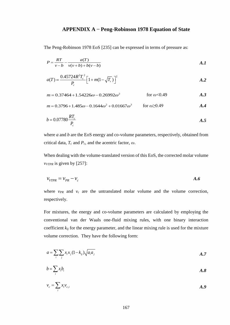
167
APPENDIX A Peng-Robinson 1978 Equation of State
The Peng-Robinson 1978 EoS [235] can be expressed in terms of pressure as:
( )
( ) ( )
RT a TP
v b v v b b v b
A.1
2 220.45724
( ) 1 (1 )cr
c
R Ta T m T
P
A.2
20.37464 1.54226 0.26992m for ω<0.49 A.3
2 30.3796 1.485 0.1644 0.01667m for ω≥0.49 A.4
0.07780 c
c
RTb
P A.5
where a and b are the EoS energy and co-volume parameters, respectively, obtained from
critical data, Tc and Pc, and the acentric factor, ω.
When dealing with the volume-translated version of this EoS, the corrected molar volume
vVTPR is given by [257]:
VTPR PR cv v v A.6
where vPR and vc are the untranslated molar volume and the volume correction,
respectively.
For mixtures, the energy and co-volume parameters are calculated by employing the
conventional van der Waals one-fluid mixing rules, with one binary interaction
coefficient kij for the energy parameter, and the linear mixing rule is used for the mixture
volume correction. They have the following form:
(1 )i j ij i j
i j
a x x k a a A.7
i i
i
b x b A.8
,c i c i
i
v x v A.9
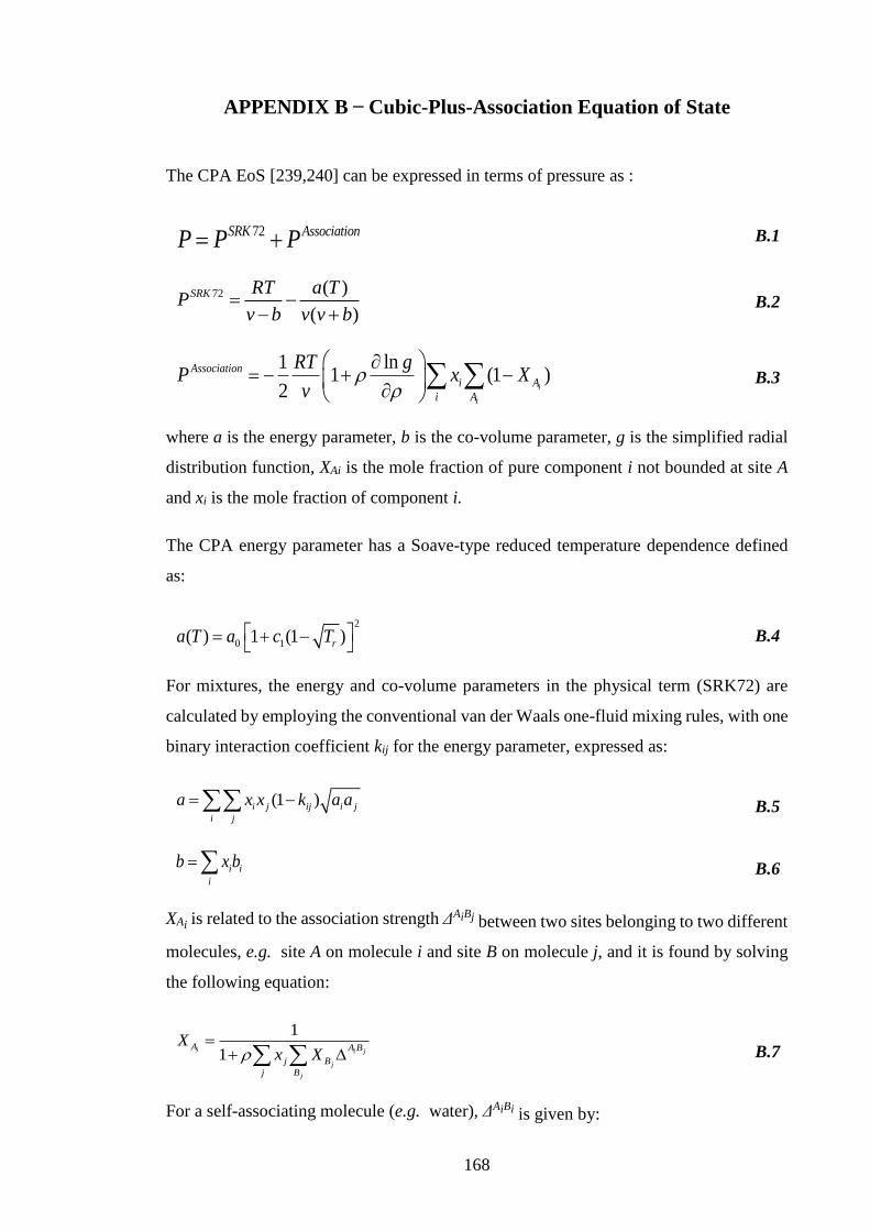
168
APPENDIX B Cubic-Plus-Association Equation of State
The CPA EoS [239,240] can be expressed in terms of pressure as :
72SRK AssociationP P P B.1
72 ( )
( )
SRK RT a TP
v b v v b
B.2
1 ln1 (1 )
2 i
i
Association
i A
i A
RT gP x X
v
B.3
where a is the energy parameter, b is the co-volume parameter, g is the simplified radial
distribution function, XAi is the mole fraction of pure component i not bounded at site A
and xi is the mole fraction of component i.
The CPA energy parameter has a Soave-type reduced temperature dependence defined
as:
2
0 1( ) 1 (1 )ra T a c T B.4
For mixtures, the energy and co-volume parameters in the physical term (SRK72) are
calculated by employing the conventional van der Waals one-fluid mixing rules, with one
binary interaction coefficient kij for the energy parameter, expressed as:
(1 )i j ij i j
i j
a x x k a a B.5
i i
i
b x b B.6
XAi is related to the association strength ΔAiBj between two sites belonging to two different
molecules, e.g. site A on molecule i and site B on molecule j, and it is found by solving
the following equation:
1
1i i j
j
j
A A B
j B
j B
Xx X
B.7
For a self-associating molecule (e.g. water), ΔAiBi is given by:
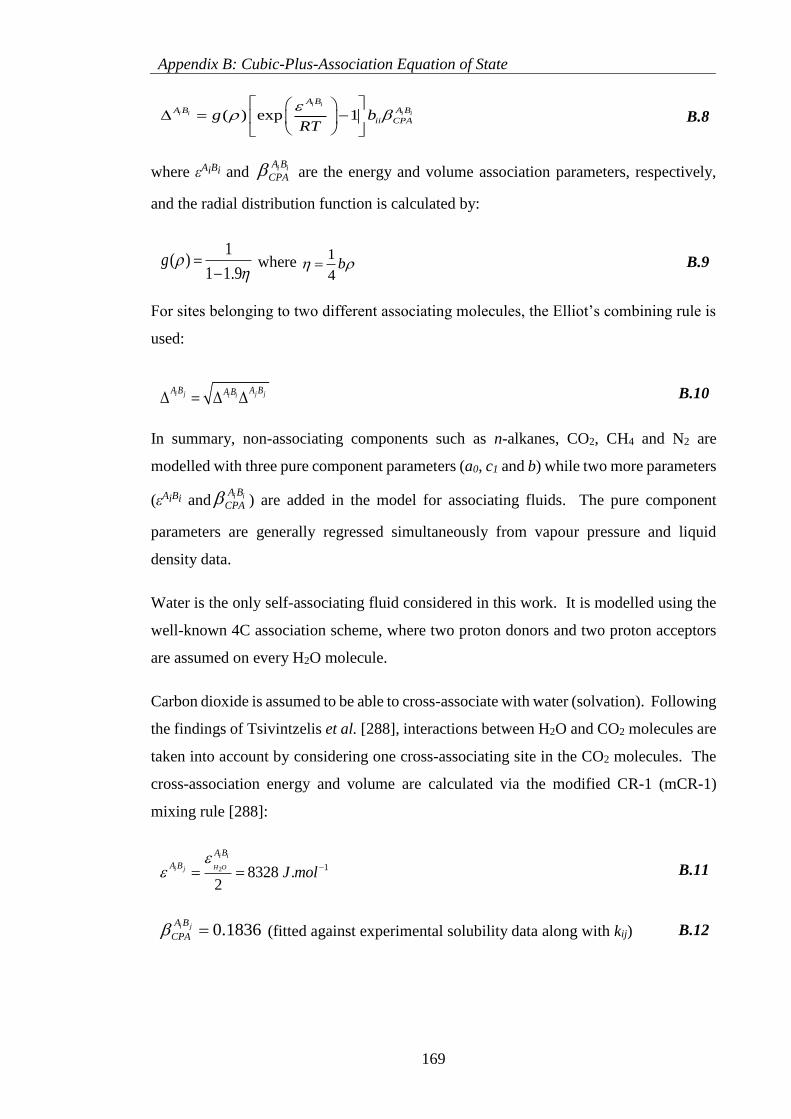
Appendix B: Cubic-Plus-Association Equation of State
169
( ) exp 1i i
i i i i
A BA B A B
ii CPAg bRT
B.8
where εAiBi and i iA B
CPA are the energy and volume association parameters, respectively,
and the radial distribution function is calculated by:
1( )
1 1.9g
where
1
4b B.9
For sites belonging to two different associating molecules, the Elliot’s combining rule is
used:
i j j ji iA B A BA B
B.10
In summary, non-associating components such as n-alkanes, CO2, CH4 and N2 are
modelled with three pure component parameters (a0, c1 and b) while two more parameters
(εAiBi and i iA B
CPA ) are added in the model for associating fluids. The pure component
parameters are generally regressed simultaneously from vapour pressure and liquid
density data.
Water is the only self-associating fluid considered in this work. It is modelled using the
well-known 4C association scheme, where two proton donors and two proton acceptors
are assumed on every H2O molecule.
Carbon dioxide is assumed to be able to cross-associate with water (solvation). Following
the findings of Tsivintzelis et al. [288], interactions between H2O and CO2 molecules are
taken into account by considering one cross-associating site in the CO2 molecules. The
cross-association energy and volume are calculated via the modified CR-1 (mCR-1)
mixing rule [288]:
2 1
28328 .
i i
H Oi j
A B
A BJ mol
B.11
0.1836i jA B
CPA (fitted against experimental solubility data along with kij) B.12
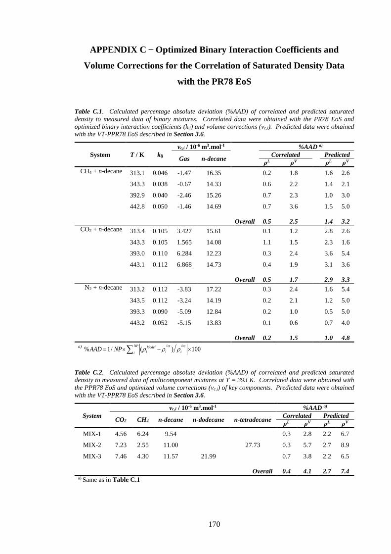
170
APPENDIX C Optimized Binary Interaction Coefficients and
Volume Corrections for the Correlation of Saturated Density Data
with the PR78 EoS
Table C.1. Calculated percentage absolute deviation (%AAD) of correlated and predicted saturated
density to measured data of binary mixtures. Correlated data were obtained with the PR78 EoS and
optimized binary interaction coefficients (kij) and volume corrections (vc,i). Predicted data were obtained
with the VT-PPR78 EoS described in Section 3.6.
System T / K kij
vc,i / 10-6 m3.mol-1 %AAD a)
Gas n-decane Correlated
Predicted
ρL ρV ρL ρV
CH4 + n-decane 313.1 0.046 -1.47 16.35 0.2 1.8 1.6 2.6
343.3 0.038 -0.67 14.33 0.6 2.2 1.4 2.1
392.9 0.040 -2.46 15.26 0.7 2.3 1.0 3.0
442.8 0.050 -1.46 14.69 0.7 3.6 1.5 5.0
Overall 0.5 2.5 1.4 3.2
CO2 + n-decane 313.4 0.105 3.427 15.61 0.1 1.2 2.8 2.6
343.3 0.105 1.565 14.08 1.1 1.5 2.3 1.6
393.0 0.110 6.284 12.23 0.3 2.4 3.6 5.4
443.1 0.112 6.868 14.73 0.4 1.9 3.1 3.6
Overall 0.5 1.7 2.9 3.3
N2 + n-decane 313.2 0.112 -3.83 17.22 0.3 2.4 1.6 5.4
343.5 0.112 -3.24 14.19 0.2 2.1 1.2 5.0
393.3 0.090 -5.09 12.84 0.2 1.0 0.5 5.0
443.2 0.052 -5.15 13.83 0.1 0.6 0.7 4.0
Overall 0.2 1.5 1.0 4.8
a) % 1/ ( ) 100Exp ExpNP Model
i i iiAAD NP
Table C.2. Calculated percentage absolute deviation (%AAD) of correlated and predicted saturated
density to measured data of multicomponent mixtures at T = 393 K. Correlated data were obtained with
the PPR78 EoS and optimized volume corrections (vc,i) of key components. Predicted data were obtained
with the VT-PPR78 EoS described in Section 3.6.
System
vc,i / 10-6 m3.mol-1 %AAD a)
CO2 CH4 n-decane n-dodecane n-tetradecane Correlated Predicted
ρL ρV ρL ρV
MIX-1 4.56 6.24 9.54 0.3 2.8 2.2 6.7
MIX-2 7.23 2.55 11.00 27.73 0.3 5.7 2.7 8.9
MIX-3 7.46 4.30 11.57 21.99 0.7 3.8 2.2 6.5
Overall 0.4 4.1 2.7 7.4 a) Same as in Table C.1
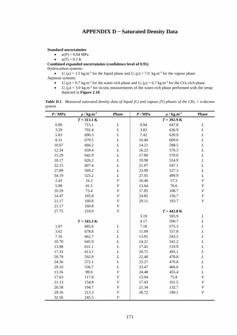
171
APPENDIX D Saturated Density Data
Standard uncertainties
u(P) = 0.04 MPa
u(T) = 0.1 K
Combined expanded uncertainties (confidence level of 0.95)
Hydrocarbon systems:
Uc (ρ) = 1.5 kg.m-3 for the liquid phase and Uc (ρ) = 7.0 kg.m-3 for the vapour phase
Aqueous systems:
Uc (ρ) = 0.7 kg.m-3 for the water-rich phase and Uc (ρ) = 6.7 kg.m-3 for the CO2-rich phase.
Uc (ρ) = 3.0 kg.m-3 for in-situ measurements of the water-rich phase performed with the setup
depicted in Figure 2.10.
Table D.1. Measured saturated density data of liquid (L) and vapour (V) phases of the CH4 + n-decane
system.
P / MPa ρ / kg.m-3 Phase P / MPa ρ / kg.m-3 Phase
T = 313.1 K T = 392.9 K
0.89 715.1 L 0.94 647.8 L
3.29 702.4 L 3.83 636.9 L
5.83 690.3 L 7.42 620.9 L
8.31 679.5 L 10.40 609.0 L
10.67 666.2 L 14.21 588.5 L
12.34 659.4 L 16.23 576.3 L
15.29 642.9 L 17.80 570.0 L
18.17 626.2 L 19.98 554.9 L
22.15 607.4 L 21.07 547.1 L
27.89 569.2 L 23.90 527.3 L
34.19 525.2 L 27.05 499.9 L
2.43 16.3 V 10.46 57.3 V
5.98 41.5 V 13.64 76.6 V
10.29 73.4 V 17.85 108.7 V
14.47 105.8 V 24.85 156.7 V
21.17 160.8 V 29.11 193.7 V
21.17 160.8 V
27.75 218.0 V T = 442.8 K
3.19 593.9 L
T = 343.3 K 4.17 590.7 L
1.87 685.6 L 7.18 575.3 L
3.62 678.8 L 11.09 557.8 L
7.10 662.7 L 13.91 543.5 L
10.70 645.9 L 14.21 541.2 L
13.98 631.1 L 17.41 519.9 L
17.33 613.1 L 20.71 495.1 L
20.79 592.9 L 22.48 478.8 L
24.36 572.1 L 23.27 470.8 L
29.10 536.7 L 23.47 466.6 L
13.16 89.0 V 24.48 455.4 L
17.63 117.8 V 13.94 75.8 V
21.13 154.8 V 17.43 101.5 V
26.58 194.7 V 21.34 132.7 V
29.16 213.3 V 26.72 190.1 V
32.56 245.5 V
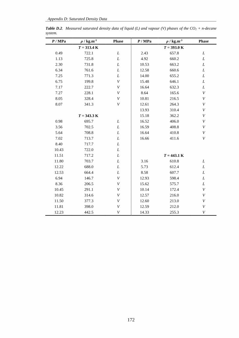
Appendix D: Saturated Density Data
172
Table D.2. Measured saturated density data of liquid (L) and vapour (V) phases of the CO2 + n-decane
system.
P / MPa ρ / kg.m-3 Phase P / MPa ρ / kg.m-3 Phase
T = 313.4 K T = 393.0 K
0.49 722.1 L 2.43 657.8 L
1.13 725.8 L 4.92 660.2 L
2.30 731.8 L 10.53 663.2 L
6.34 761.6 L 12.58 660.6 L
7.25 771.3 L 14.00 655.2 L
6.75 199.8 V 15.48 646.1 L
7.17 222.7 V 16.64 632.3 L
7.27 228.1 V 8.64 165.6 V
8.05 328.4 V 10.81 216.5 V
8.07 341.3 V 12.61 264.3 V
13.93 310.4 V
T = 343.3 K 15.18 362.2 V
0.98 695.7 L 16.52 406.0 V
3.56 702.5 L 16.59 408.8 V
5.64 708.8 L 16.64 410.8 V
7.02 713.7 L 16.66 411.6 V
8.40 717.7 L
10.43 722.0 L
11.51 717.2 L T = 443.1 K
11.80 703.7 L 3.16 610.8 L
12.22 688.0 L 5.73 612.4 L
12.53 664.4 L 8.58 607.7 L
6.94 146.7 V 12.93 598.4 L
8.36 206.5 V 15.62 575.7 L
10.45 291.1 V 10.14 172.4 V
10.82 314.6 V 12.57 216.0 V
11.50 377.3 V 12.60 213.0 V
11.81 398.0 V 12.59 212.0 V
12.23 442.5 V 14.33 255.3 V
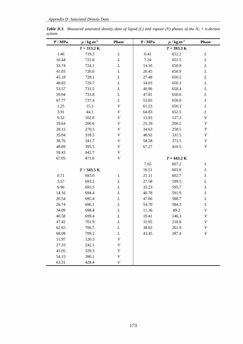
Appendix D: Saturated Density Data
173
Table D.3. Measured saturated density data of liquid (L) and vapour (V) phases of the N2 + n-decane
system.
P / MPa ρ / kg.m-3 Phase P / MPa ρ / kg.m-3 Phase
T = 313.2 K T = 393.3 K
1.46 719.3 L 0.41 652.2 L
10.44 721.8 L 7.24 651.5 L
33.74 724.1 L 14.16 650.9 L
41.03 726.6 L 20.45 650.9 L
45.18 728.1 L 27.48 650.2 L
48.83 729.7 L 34.03 650.3 L
53.57 731.5 L 40.96 650.4 L
59.94 733.8 L 47.81 650.6 L
67.77 737.4 L 53.83 650.6 L
1.25 15.3 V 61.53 650.3 L
3.91 44.1 V 64.83 652.5 L
9.32 102.0 V 13.93 117.3 V
19.64 200.6 V 25.29 200.5 V
28.12 270.3 V 34.63 258.5 V
35.04 318.5 V 48.92 331.5 V
38.76 341.7 V 58.58 373.5 V
48.69 395.5 V 67.27 410.5 V
59.43 442.7 V
67.05 471.0 V T = 443.2 K
7.65 607.2 L
T = 343.5 K 16.51 603.8 L
0.71 693.0 L 21.11 602.7 L
3.57 693.2 L 27.58 599.5 L
6.96 693.5 L 35.23 595.7 L
14.16 694.4 L 40.78 591.9 L
20.54 695.4 L 47.06 588.7 L
26.74 696.1 L 54.70 584.3 L
34.09 698.4 L 11.36 89.2 V
40.58 699.4 L 19.41 146.3 V
47.42 701.9 L 31.05 218.8 V
62.65 706.7 L 38.02 261.9 V
68.08 709.2 L 43.45 287.4 V
11.97 120.3 V
27.33 242.1 V
41.05 329.3 V
54.15 390.1 V
63.31 428.4 V
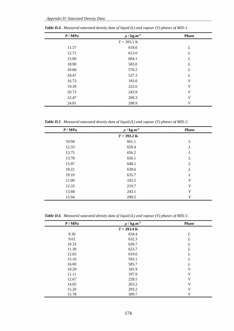
Appendix D: Saturated Density Data
174
Table D.4. Measured saturated density data of liquid (L) and vapour (V) phases of MIX-1.
P / MPa ρ / kg.m-3 Phase
T = 393.1 K
11.57 618.6 L
12.71 613.0 L
15.00 604.1 L
18.90 583.0 L
20.68 570.2 L
24.47 537.3 L
16.73 183.0 V
19.39 222.6 V
20.73 243.9 V
22.47 269.3 V
24.01 298.9 V
Table D.5. Measured saturated density data of liquid (L) and vapour (V) phases of MIX-2.
P / MPa ρ / kg.m-3 Phase
T = 393.2 K
10.94 661.1 L
12.33 659.4 L
13.75 656.2 L
13.78 656.1 L
15.97 648.1 L
18.22 639.6 L
19.10 635.7 L
11.00 192.5 V
12.33 219.7 V
13.68 243.1 V
15.94 299.5 V
Table D.6. Measured saturated density data of liquid (L) and vapour (V) phases of MIX-3.
P / MPa ρ / kg.m-3 Phase
T = 393.4 K
9.36 634.4 L
9.61 632.3 L
10.33 626.7 L
11.30 623.7 L
12.63 619.6 L
15.10 593.1 L
16.00 585.7 L
10.29 181.9 V
11.11 197.9 V
12.67 228.5 V
14.05 263.2 V
15.20 293.2 V
15.78 309.7 V
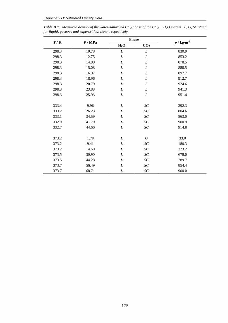
Appendix D: Saturated Density Data
175
Table D.7. Measured density of the water-saturated CO2 phase of the CO2 + H2O system. L, G, SC stand
for liquid, gaseous and supercritical state, respectively.
T / K P / MPa Phase
ρ / kg∙m-3
H2O CO2
298.3 10.78 L L 830.9
298.3 12.75 L L 853.2
298.3 14.88 L L 878.5
298.3 15.08 L L 880.5
298.3 16.97 L L 897.7
298.3 18.96 L L 912.7
298.3 20.79 L L 924.6
298.3 23.83 L L 941.3
298.3 25.93 L L 951.4
333.4 9.96 L SC 292.3
333.2 26.23 L SC 804.6
333.1 34.59 L SC 863.0
332.9 41.70 L SC 900.9
332.7 44.66 L SC 914.8
373.2 1.78 L G 33.0
373.2 9.41 L SC 180.3
373.2 14.60 L SC 323.2
373.5 30.90 L SC 678.0
373.5 44.28 L SC 789.7
373.7 56.49 L SC 854.4
373.7 68.71 L SC 900.0
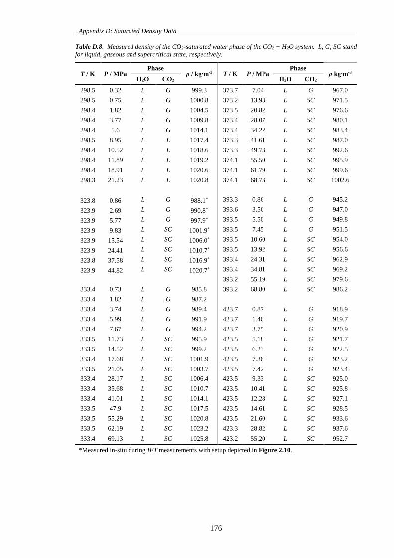
Appendix D: Saturated Density Data
176
Table D.8. Measured density of the CO2-saturated water phase of the CO2 + H2O system. L, G, SC stand
for liquid, gaseous and supercritical state, respectively.
T / K P / MPa Phase
ρ / kg∙m-3 T / K P / MPa Phase
ρ kg∙m-3 H2O CO2 H2O CO2
298.5 0.32 L G 999.3 373.7 7.04 L G 967.0
298.5 0.75 L G 1000.8 373.2 13.93 L SC 971.5
298.4 1.82 L G 1004.5 373.5 20.82 L SC 976.6
298.4 3.77 L G 1009.8 373.4 28.07 L SC 980.1
298.4 5.6 L G 1014.1 373.4 34.22 L SC 983.4
298.5 8.95 L L 1017.4 373.3 41.61 L SC 987.0
298.4 10.52 L L 1018.6 373.3 49.73 L SC 992.6
298.4 11.89 L L 1019.2 374.1 55.50 L SC 995.9
298.4 18.91 L L 1020.6 374.1 61.79 L SC 999.6
298.3 21.23 L L 1020.8 374.1 68.73 L SC 1002.6
323.8 0.86 L G 988.1* 393.3 0.86 L G 945.2
323.9 2.69 L G 990.8* 393.6 3.56 L G 947.0
323.9 5.77 L G 997.9* 393.5 5.50 L G 949.8
323.9 9.83 L SC 1001.9* 393.5 7.45 L G 951.5
323.9 15.54 L SC 1006.0* 393.5 10.60 L SC 954.0
323.9 24.41 L SC 1010.7* 393.5 13.92 L SC 956.6
323.8 37.58 L SC 1016.9* 393.4 24.31 L SC 962.9
323.9 44.82 L SC 1020.7* 393.4 34.81 L SC 969.2
393.2 55.19 L SC 979.6
333.4 0.73 L G 985.8 393.2 68.80 L SC 986.2
333.4 1.82 L G 987.2
333.4 3.74 L G 989.4 423.7 0.87 L G 918.9
333.4 5.99 L G 991.9 423.7 1.46 L G 919.7
333.4 7.67 L G 994.2 423.7 3.75 L G 920.9
333.5 11.73 L SC 995.9 423.5 5.18 L G 921.7
333.5 14.52 L SC 999.2 423.5 6.23 L G 922.5
333.4 17.68 L SC 1001.9 423.5 7.36 L G 923.2
333.5 21.05 L SC 1003.7 423.5 7.42 L G 923.4
333.4 28.17 L SC 1006.4 423.5 9.33 L SC 925.0
333.4 35.68 L SC 1010.7 423.5 10.41 L SC 925.8
333.4 41.01 L SC 1014.1 423.5 12.28 L SC 927.1
333.5 47.9 L SC 1017.5 423.5 14.61 L SC 928.5
333.5 55.29 L SC 1020.8 423.5 21.60 L SC 933.6
333.5 62.19 L SC 1023.2 423.3 28.82 L SC 937.6
333.4 69.13 L SC 1025.8 423.2 55.20 L SC 952.7
*Measured in-situ during IFT measurements with setup depicted in Figure 2.10.
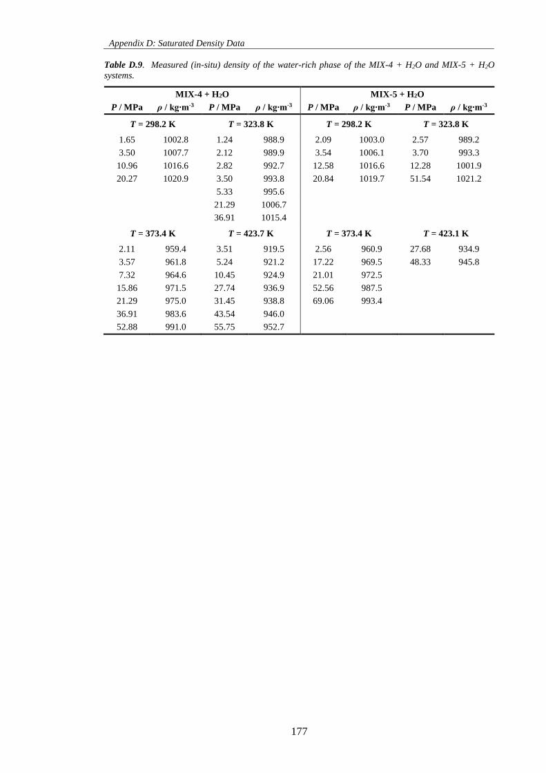
Appendix D: Saturated Density Data
177
Table D.9. Measured (in-situ) density of the water-rich phase of the MIX-4 + H2O and MIX-5 + H2O
systems.
MIX-4 + H2O MIX-5 + H2O
P / MPa ρ / kg∙m-3 P / MPa ρ / kg∙m-3 P / MPa ρ / kg∙m-3 P / MPa ρ / kg∙m-3
T = 298.2 K T = 323.8 K T = 298.2 K T = 323.8 K
1.65 1002.8 1.24 988.9 2.09 1003.0 2.57 989.2
3.50 1007.7 2.12 989.9 3.54 1006.1 3.70 993.3
10.96 1016.6 2.82 992.7 12.58 1016.6 12.28 1001.9
20.27 1020.9 3.50 993.8 20.84 1019.7 51.54 1021.2
5.33 995.6
21.29 1006.7
36.91 1015.4
T = 373.4 K T = 423.7 K T = 373.4 K T = 423.1 K
2.11 959.4 3.51 919.5 2.56 960.9 27.68 934.9
3.57 961.8 5.24 921.2 17.22 969.5 48.33 945.8
7.32 964.6 10.45 924.9 21.01 972.5
15.86 971.5 27.74 936.9 52.56 987.5
21.29 975.0 31.45 938.8 69.06 993.4
36.91 983.6 43.54 946.0
52.88 991.0 55.75 952.7
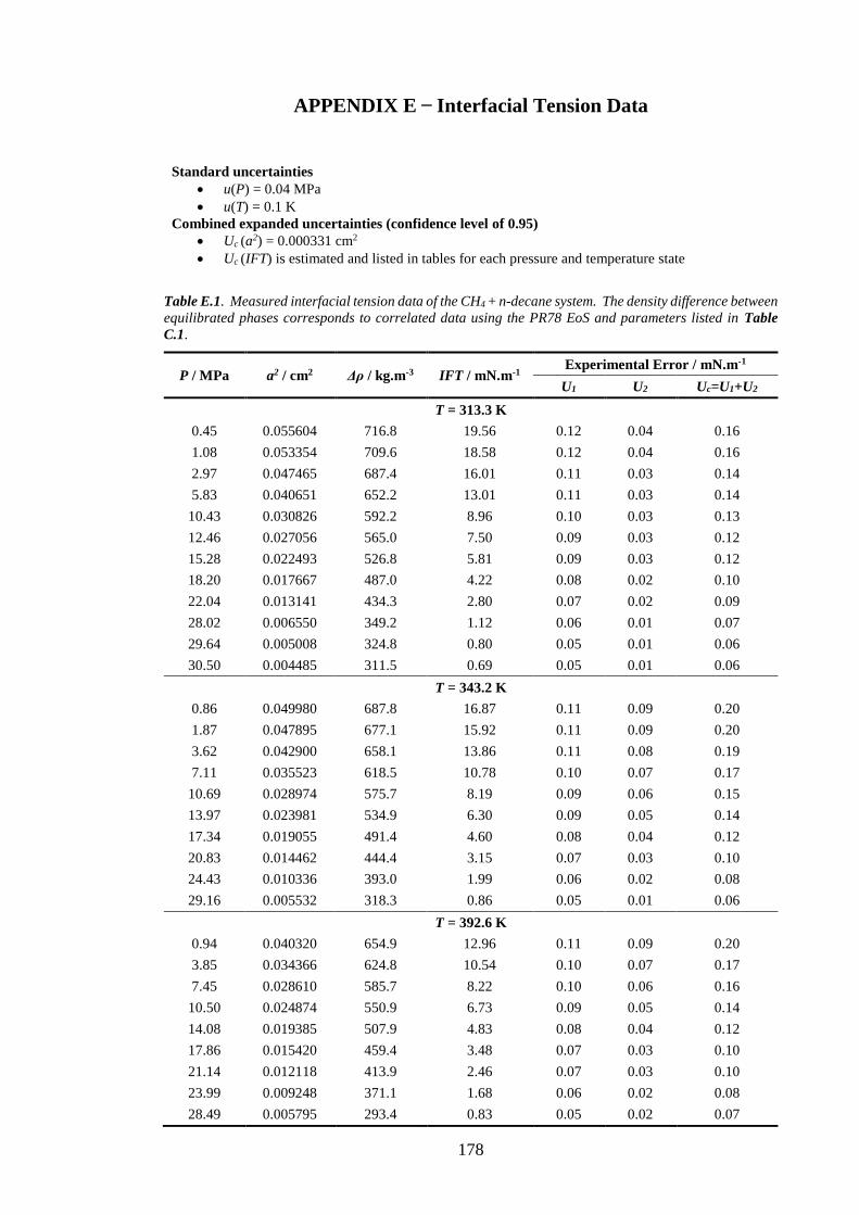
178
APPENDIX E Interfacial Tension Data
Standard uncertainties
u(P) = 0.04 MPa
u(T) = 0.1 K
Combined expanded uncertainties (confidence level of 0.95)
Uc (a2) = 0.000331 cm2
Uc (IFT) is estimated and listed in tables for each pressure and temperature state
Table E.1. Measured interfacial tension data of the CH4 + n-decane system. The density difference between
equilibrated phases corresponds to correlated data using the PR78 EoS and parameters listed in Table
C.1.
P / MPa a2 / cm2 Δρ / kg.m-3 IFT / mN.m-1 Experimental Error / mN.m-1
U1 U2 Uc=U1+U2
T = 313.3 K
0.45 0.055604 716.8 19.56 0.12 0.04 0.16
1.08 0.053354 709.6 18.58 0.12 0.04 0.16
2.97 0.047465 687.4 16.01 0.11 0.03 0.14
5.83 0.040651 652.2 13.01 0.11 0.03 0.14
10.43 0.030826 592.2 8.96 0.10 0.03 0.13
12.46 0.027056 565.0 7.50 0.09 0.03 0.12
15.28 0.022493 526.8 5.81 0.09 0.03 0.12
18.20 0.017667 487.0 4.22 0.08 0.02 0.10
22.04 0.013141 434.3 2.80 0.07 0.02 0.09
28.02 0.006550 349.2 1.12 0.06 0.01 0.07
29.64 0.005008 324.8 0.80 0.05 0.01 0.06
30.50 0.004485 311.5 0.69 0.05 0.01 0.06
T = 343.2 K
0.86 0.049980 687.8 16.87 0.11 0.09 0.20
1.87 0.047895 677.1 15.92 0.11 0.09 0.20
3.62 0.042900 658.1 13.86 0.11 0.08 0.19
7.11 0.035523 618.5 10.78 0.10 0.07 0.17
10.69 0.028974 575.7 8.19 0.09 0.06 0.15
13.97 0.023981 534.9 6.30 0.09 0.05 0.14
17.34 0.019055 491.4 4.60 0.08 0.04 0.12
20.83 0.014462 444.4 3.15 0.07 0.03 0.10
24.43 0.010336 393.0 1.99 0.06 0.02 0.08
29.16 0.005532 318.3 0.86 0.05 0.01 0.06
T = 392.6 K
0.94 0.040320 654.9 12.96 0.11 0.09 0.20
3.85 0.034366 624.8 10.54 0.10 0.07 0.17
7.45 0.028610 585.7 8.22 0.10 0.06 0.16
10.50 0.024874 550.9 6.73 0.09 0.05 0.14
14.08 0.019385 507.9 4.83 0.08 0.04 0.12
17.86 0.015420 459.4 3.48 0.07 0.03 0.10
21.14 0.012118 413.9 2.46 0.07 0.03 0.10
23.99 0.009248 371.1 1.68 0.06 0.02 0.08
28.49 0.005795 293.4 0.83 0.05 0.02 0.07
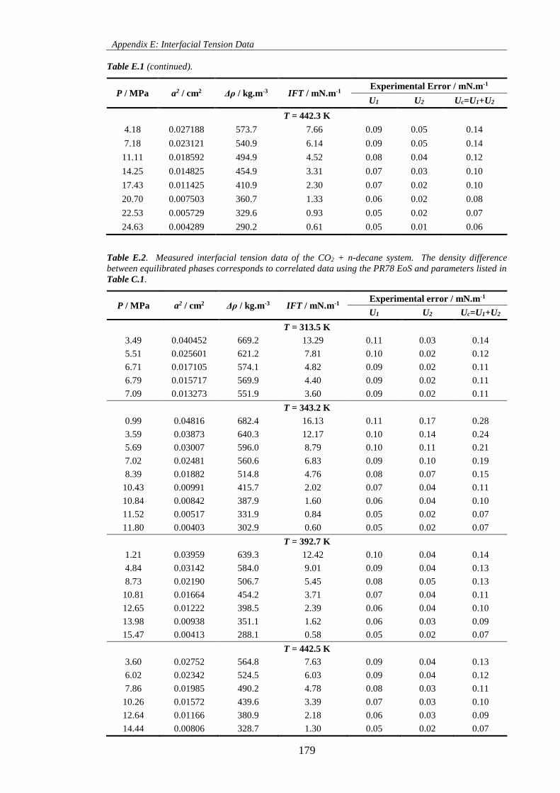
Appendix E: Interfacial Tension Data
179
Table E.1 (continued).
P / MPa a2 / cm2 Δρ / kg.m-3 IFT / mN.m-1 Experimental Error / mN.m-1
U1 U2 Uc=U1+U2
T = 442.3 K
4.18 0.027188 573.7 7.66 0.09 0.05 0.14
7.18 0.023121 540.9 6.14 0.09 0.05 0.14
11.11 0.018592 494.9 4.52 0.08 0.04 0.12
14.25 0.014825 454.9 3.31 0.07 0.03 0.10
17.43 0.011425 410.9 2.30 0.07 0.02 0.10
20.70 0.007503 360.7 1.33 0.06 0.02 0.08
22.53 0.005729 329.6 0.93 0.05 0.02 0.07
24.63 0.004289 290.2 0.61 0.05 0.01 0.06
Table E.2. Measured interfacial tension data of the CO2 + n-decane system. The density difference
between equilibrated phases corresponds to correlated data using the PR78 EoS and parameters listed in
Table C.1.
P / MPa a2 / cm2 Δρ / kg.m-3 IFT / mN.m-1 Experimental error / mN.m-1
U1 U2 Uc=U1+U2
T = 313.5 K
3.49 0.040452 669.2 13.29 0.11 0.03 0.14
5.51 0.025601 621.2 7.81 0.10 0.02 0.12
6.71 0.017105 574.1 4.82 0.09 0.02 0.11
6.79 0.015717 569.9 4.40 0.09 0.02 0.11
7.09 0.013273 551.9 3.60 0.09 0.02 0.11
T = 343.2 K
0.99 0.04816 682.4 16.13 0.11 0.17 0.28
3.59 0.03873 640.3 12.17 0.10 0.14 0.24
5.69 0.03007 596.0 8.79 0.10 0.11 0.21
7.02 0.02481 560.6 6.83 0.09 0.10 0.19
8.39 0.01882 514.8 4.76 0.08 0.07 0.15
10.43 0.00991 415.7 2.02 0.07 0.04 0.11
10.84 0.00842 387.9 1.60 0.06 0.04 0.10
11.52 0.00517 331.9 0.84 0.05 0.02 0.07
11.80 0.00403 302.9 0.60 0.05 0.02 0.07
T = 392.7 K
1.21 0.03959 639.3 12.42 0.10 0.04 0.14
4.84 0.03142 584.0 9.01 0.09 0.04 0.13
8.73 0.02190 506.7 5.45 0.08 0.05 0.13
10.81 0.01664 454.2 3.71 0.07 0.04 0.11
12.65 0.01222 398.5 2.39 0.06 0.04 0.10
13.98 0.00938 351.1 1.62 0.06 0.03 0.09
15.47 0.00413 288.1 0.58 0.05 0.02 0.07
T = 442.5 K
3.60 0.02752 564.8 7.63 0.09 0.04 0.13
6.02 0.02342 524.5 6.03 0.09 0.04 0.12
7.86 0.01985 490.2 4.78 0.08 0.03 0.11
10.26 0.01572 439.6 3.39 0.07 0.03 0.10
12.64 0.01166 380.9 2.18 0.06 0.03 0.09
14.44 0.00806 328.7 1.30 0.05 0.02 0.07
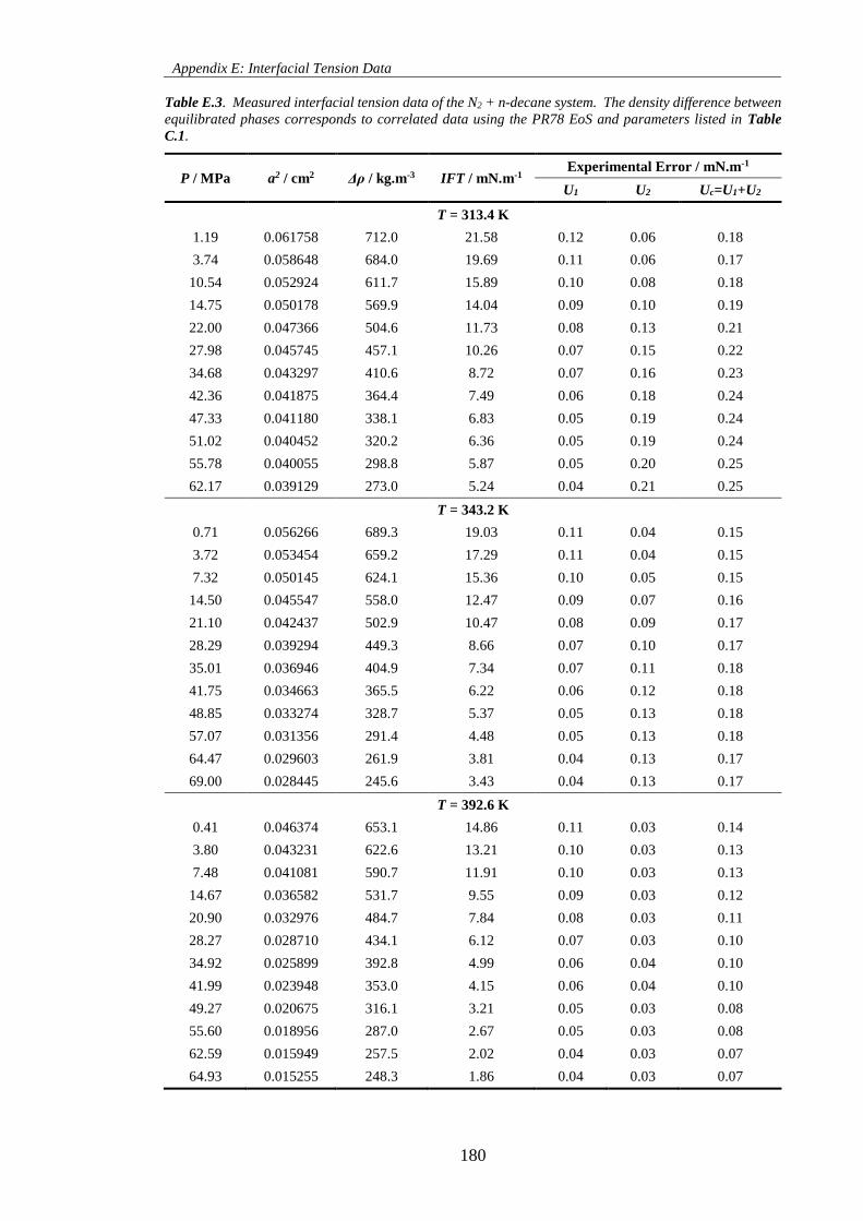
Appendix E: Interfacial Tension Data
180
Table E.3. Measured interfacial tension data of the N2 + n-decane system. The density difference between
equilibrated phases corresponds to correlated data using the PR78 EoS and parameters listed in Table
C.1.
P / MPa a2 / cm2 Δρ / kg.m-3 IFT / mN.m-1 Experimental Error / mN.m-1
U1 U2 Uc=U1+U2
T = 313.4 K
1.19 0.061758 712.0 21.58 0.12 0.06 0.18
3.74 0.058648 684.0 19.69 0.11 0.06 0.17
10.54 0.052924 611.7 15.89 0.10 0.08 0.18
14.75 0.050178 569.9 14.04 0.09 0.10 0.19
22.00 0.047366 504.6 11.73 0.08 0.13 0.21
27.98 0.045745 457.1 10.26 0.07 0.15 0.22
34.68 0.043297 410.6 8.72 0.07 0.16 0.23
42.36 0.041875 364.4 7.49 0.06 0.18 0.24
47.33 0.041180 338.1 6.83 0.05 0.19 0.24
51.02 0.040452 320.2 6.36 0.05 0.19 0.24
55.78 0.040055 298.8 5.87 0.05 0.20 0.25
62.17 0.039129 273.0 5.24 0.04 0.21 0.25
T = 343.2 K
0.71 0.056266 689.3 19.03 0.11 0.04 0.15
3.72 0.053454 659.2 17.29 0.11 0.04 0.15
7.32 0.050145 624.1 15.36 0.10 0.05 0.15
14.50 0.045547 558.0 12.47 0.09 0.07 0.16
21.10 0.042437 502.9 10.47 0.08 0.09 0.17
28.29 0.039294 449.3 8.66 0.07 0.10 0.17
35.01 0.036946 404.9 7.34 0.07 0.11 0.18
41.75 0.034663 365.5 6.22 0.06 0.12 0.18
48.85 0.033274 328.7 5.37 0.05 0.13 0.18
57.07 0.031356 291.4 4.48 0.05 0.13 0.18
64.47 0.029603 261.9 3.81 0.04 0.13 0.17
69.00 0.028445 245.6 3.43 0.04 0.13 0.17
T = 392.6 K
0.41 0.046374 653.1 14.86 0.11 0.03 0.14
3.80 0.043231 622.6 13.21 0.10 0.03 0.13
7.48 0.041081 590.7 11.91 0.10 0.03 0.13
14.67 0.036582 531.7 9.55 0.09 0.03 0.12
20.90 0.032976 484.7 7.84 0.08 0.03 0.11
28.27 0.028710 434.1 6.12 0.07 0.03 0.10
34.92 0.025899 392.8 4.99 0.06 0.04 0.10
41.99 0.023948 353.0 4.15 0.06 0.04 0.10
49.27 0.020675 316.1 3.21 0.05 0.03 0.08
55.60 0.018956 287.0 2.67 0.05 0.03 0.08
62.59 0.015949 257.5 2.02 0.04 0.03 0.07
64.93 0.015255 248.3 1.86 0.04 0.03 0.07
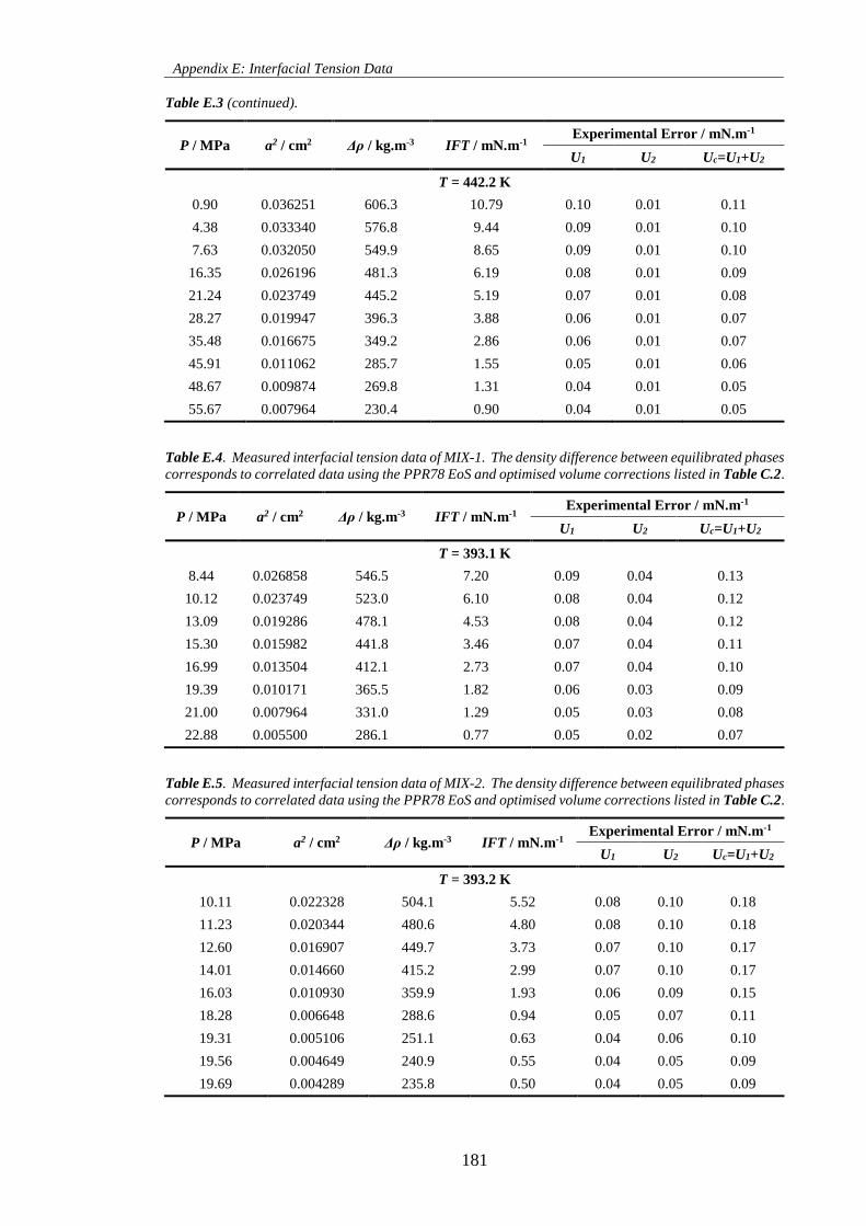
Appendix E: Interfacial Tension Data
181
Table E.3 (continued).
P / MPa a2 / cm2 Δρ / kg.m-3 IFT / mN.m-1 Experimental Error / mN.m-1
U1 U2 Uc=U1+U2
T = 442.2 K
0.90 0.036251 606.3 10.79 0.10 0.01 0.11
4.38 0.033340 576.8 9.44 0.09 0.01 0.10
7.63 0.032050 549.9 8.65 0.09 0.01 0.10
16.35 0.026196 481.3 6.19 0.08 0.01 0.09
21.24 0.023749 445.2 5.19 0.07 0.01 0.08
28.27 0.019947 396.3 3.88 0.06 0.01 0.07
35.48 0.016675 349.2 2.86 0.06 0.01 0.07
45.91 0.011062 285.7 1.55 0.05 0.01 0.06
48.67 0.009874 269.8 1.31 0.04 0.01 0.05
55.67 0.007964 230.4 0.90 0.04 0.01 0.05
Table E.4. Measured interfacial tension data of MIX-1. The density difference between equilibrated phases
corresponds to correlated data using the PPR78 EoS and optimised volume corrections listed in Table C.2.
P / MPa a2 / cm2 Δρ / kg.m-3 IFT / mN.m-1 Experimental Error / mN.m-1
U1 U2 Uc=U1+U2
T = 393.1 K
8.44 0.026858 546.5 7.20 0.09 0.04 0.13
10.12 0.023749 523.0 6.10 0.08 0.04 0.12
13.09 0.019286 478.1 4.53 0.08 0.04 0.12
15.30 0.015982 441.8 3.46 0.07 0.04 0.11
16.99 0.013504 412.1 2.73 0.07 0.04 0.10
19.39 0.010171 365.5 1.82 0.06 0.03 0.09
21.00 0.007964 331.0 1.29 0.05 0.03 0.08
22.88 0.005500 286.1 0.77 0.05 0.02 0.07
Table E.5. Measured interfacial tension data of MIX-2. The density difference between equilibrated phases
corresponds to correlated data using the PPR78 EoS and optimised volume corrections listed in Table C.2.
P / MPa a2 / cm2 Δρ / kg.m-3 IFT / mN.m-1 Experimental Error / mN.m-1
U1 U2 Uc=U1+U2
T = 393.2 K
10.11 0.022328 504.1 5.52 0.08 0.10 0.18
11.23 0.020344 480.6 4.80 0.08 0.10 0.18
12.60 0.016907 449.7 3.73 0.07 0.10 0.17
14.01 0.014660 415.2 2.99 0.07 0.10 0.17
16.03 0.010930 359.9 1.93 0.06 0.09 0.15
18.28 0.006648 288.6 0.94 0.05 0.07 0.11
19.31 0.005106 251.1 0.63 0.04 0.06 0.10
19.56 0.004649 240.9 0.55 0.04 0.05 0.09
19.69 0.004289 235.8 0.50 0.04 0.05 0.09
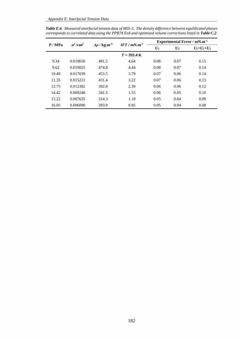
Appendix E: Interfacial Tension Data
182
Table E.6. Measured interfacial tension data of MIX-3. The density difference between equilibrated phases
corresponds to correlated data using the PPR78 EoS and optimised volume corrections listed in Table C.2.
P / MPa a2 /cm2 Δρ / kg.m-3 IFT / mN.m-1 Experimental Error / mN.m-1
U1 U2 Uc=U1+U2
T = 393.4 K
9.34 0.019650 481.5 4.64 0.08 0.07 0.15
9.62 0.019055 474.8 4.44 0.08 0.07 0.14
10.49 0.017039 453.5 3.79 0.07 0.06 0.14
11.35 0.015222 431.4 3.22 0.07 0.06 0.13
12.75 0.012382 392.8 2.39 0.06 0.06 0.12
14.42 0.009248 341.5 1.55 0.06 0.05 0.10
15.22 0.007635 314.3 1.18 0.05 0.04 0.09
16.05 0.006090 283.9 0.85 0.05 0.04 0.08
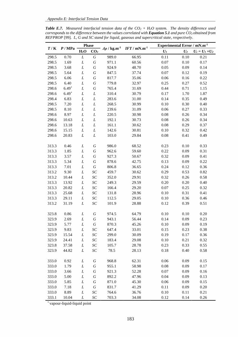
Appendix E: Interfacial Tension Data
183
Table E.7. Measured interfacial tension data of the CO2 + H2O system. The density difference used
corresponds to the difference between the values correlated with Equation 5.1 and pure CO2 obtained from
REFPROP [99]. L, G and SC stand for liquid, gaseous and supercritical state, respectively.
T / K P / MPa Phase
Δρ / kg.m-3 IFT / mN.m-1 Experimental Error / mN.m-1
H2O CO2 U1 U2 Uc = U1 +U2
298.5 0.70 L G 989.0 66.95 0.11 0.10 0.21
298.5 1.69 L G 971.1 60.56 0.07 0.10 0.17
298.5 3.68 L G 924.9 48.70 0.05 0.09 0.14
298.5 5.64 L G 847.5 37.74 0.07 0.12 0.19
298.5 6.06 L G 817.7 35.06 0.06 0.16 0.22
298.5 6.40 L G 779.8 32.97 0.25 0.27 0.52
298.6 6.49* L G 765.4 31.69 0.44 0.71 1.15
298.6 6.49* L L 310.4 30.79 0.17 1.70 1.87
298.4 6.83 L L 283.6 31.00 0.14 0.35 0.49
298.5 7.20 L L 268.5 30.99 0.10 0.30 0.40
298.5 8.10 L L 239.6 31.09 0.06 0.27 0.33
298.6 8.97 L L 220.5 30.98 0.08 0.26 0.34
298.6 10.63 L L 192.1 30.73 0.08 0.26 0.34
298.6 13.18 L L 161.1 30.62 0.08 0.29 0.37
298.6 15.15 L L 142.6 30.81 0.10 0.32 0.42
298.6 20.83 L L 103.0 29.84 0.08 0.41 0.49
313.3 0.46 L G 986.0 68.52 0.23 0.10 0.33
313.3 1.85 L G 962.6 59.60 0.22 0.09 0.31
313.3 3.57 L G 927.3 50.67 0.32 0.09 0.41
313.3 5.34 L G 878.6 42.75 0.13 0.09 0.22
313.3 7.01 L G 806.8 36.65 0.24 0.12 0.36
313.2 9.30 L SC 459.7 30.62 0.29 0.53 0.82
313.2 10.44 L SC 352.0 29.91 0.32 0.26 0.58
313.3 13.92 L SC 249.3 29.59 0.20 0.20 0.40
313.3 20.82 L SC 166.4 29.20 0.07 0.25 0.32
313.3 25.68 L SC 131.8 28.96 0.10 0.31 0.41
313.3 29.11 L SC 112.5 29.05 0.10 0.36 0.46
313.2 31.19 L SC 101.9 28.88 0.12 0.39 0.51
323.8 0.86 L G 974.5 64.79 0.10 0.10 0.20
323.9 2.69 L G 943.1 56.44 0.14 0.09 0.23
323.9 5.77 L G 870.3 45.26 0.10 0.09 0.19
323.9 9.83 L SC 647.4 33.01 0.15 0.23 0.38
323.9 15.54 L SC 299.0 30.09 0.19 0.17 0.36
323.9 24.41 L SC 183.4 29.08 0.10 0.21 0.32
323.8 37.58 L SC 105.7 28.78 0.23 0.33 0.55
323.9 44.82 L SC 78.5 28.13 0.18 0.40 0.58
333.0 0.92 L G 968.8 62.31 0.06 0.09 0.15
333.0 1.79 L G 955.1 58.98 0.08 0.09 0.17
333.0 3.66 L G 921.3 52.28 0.07 0.09 0.16
333.0 5.00 L G 892.2 47.96 0.04 0.09 0.13
333.0 5.85 L G 871.0 45.30 0.06 0.09 0.15
333.0 7.18 L G 831.7 41.29 0.11 0.09 0.20
333.0 8.89 L SC 764.6 36.76 0.10 0.11 0.21
333.1 10.04 L SC 703.3 34.08 0.12 0.14 0.26 * vapour-liquid-liquid point
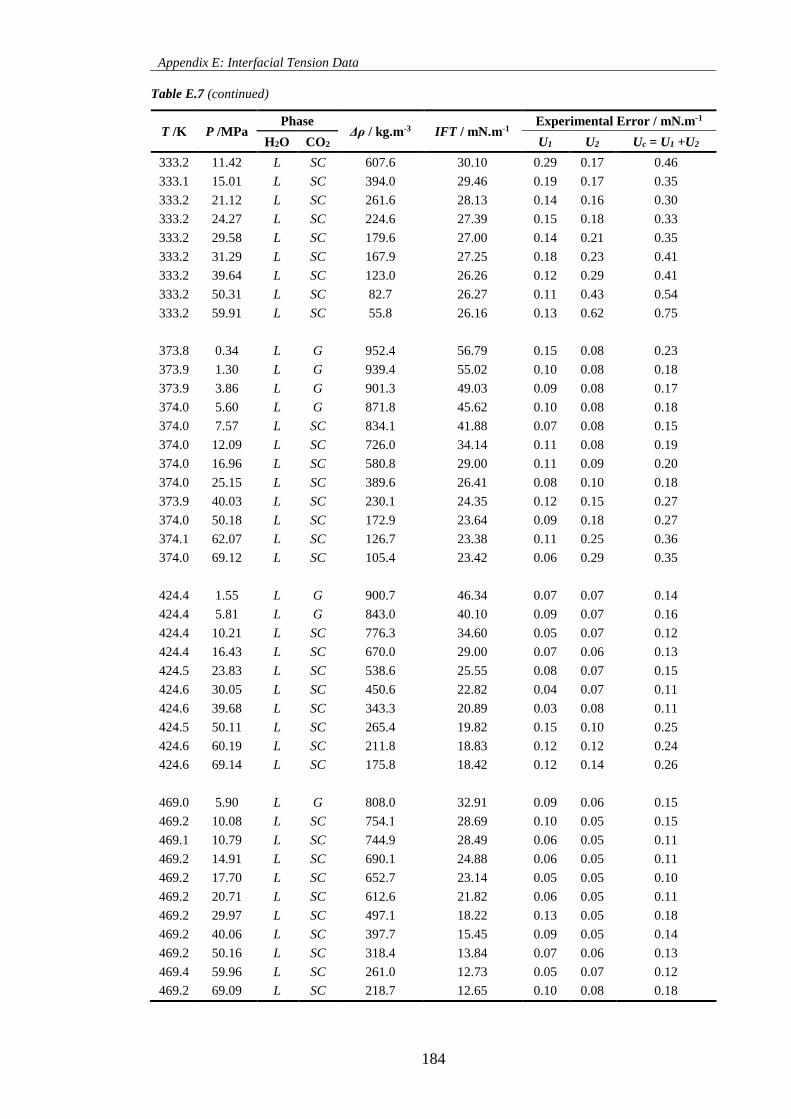
Appendix E: Interfacial Tension Data
184
Table E.7 (continued)
T /K P /MPa Phase
Δρ / kg.m-3 IFT / mN.m-1 Experimental Error / mN.m-1
H2O CO2 U1 U2 Uc = U1 +U2
333.2 11.42 L SC 607.6 30.10 0.29 0.17 0.46
333.1 15.01 L SC 394.0 29.46 0.19 0.17 0.35
333.2 21.12 L SC 261.6 28.13 0.14 0.16 0.30
333.2 24.27 L SC 224.6 27.39 0.15 0.18 0.33
333.2 29.58 L SC 179.6 27.00 0.14 0.21 0.35
333.2 31.29 L SC 167.9 27.25 0.18 0.23 0.41
333.2 39.64 L SC 123.0 26.26 0.12 0.29 0.41
333.2 50.31 L SC 82.7 26.27 0.11 0.43 0.54
333.2 59.91 L SC 55.8 26.16 0.13 0.62 0.75
373.8 0.34 L G 952.4 56.79 0.15 0.08 0.23
373.9 1.30 L G 939.4 55.02 0.10 0.08 0.18
373.9 3.86 L G 901.3 49.03 0.09 0.08 0.17
374.0 5.60 L G 871.8 45.62 0.10 0.08 0.18
374.0 7.57 L SC 834.1 41.88 0.07 0.08 0.15
374.0 12.09 L SC 726.0 34.14 0.11 0.08 0.19
374.0 16.96 L SC 580.8 29.00 0.11 0.09 0.20
374.0 25.15 L SC 389.6 26.41 0.08 0.10 0.18
373.9 40.03 L SC 230.1 24.35 0.12 0.15 0.27
374.0 50.18 L SC 172.9 23.64 0.09 0.18 0.27
374.1 62.07 L SC 126.7 23.38 0.11 0.25 0.36
374.0 69.12 L SC 105.4 23.42 0.06 0.29 0.35
424.4 1.55 L G 900.7 46.34 0.07 0.07 0.14
424.4 5.81 L G 843.0 40.10 0.09 0.07 0.16
424.4 10.21 L SC 776.3 34.60 0.05 0.07 0.12
424.4 16.43 L SC 670.0 29.00 0.07 0.06 0.13
424.5 23.83 L SC 538.6 25.55 0.08 0.07 0.15
424.6 30.05 L SC 450.6 22.82 0.04 0.07 0.11
424.6 39.68 L SC 343.3 20.89 0.03 0.08 0.11
424.5 50.11 L SC 265.4 19.82 0.15 0.10 0.25
424.6 60.19 L SC 211.8 18.83 0.12 0.12 0.24
424.6 69.14 L SC 175.8 18.42 0.12 0.14 0.26
469.0 5.90 L G 808.0 32.91 0.09 0.06 0.15
469.2 10.08 L SC 754.1 28.69 0.10 0.05 0.15
469.1 10.79 L SC 744.9 28.49 0.06 0.05 0.11
469.2 14.91 L SC 690.1 24.88 0.06 0.05 0.11
469.2 17.70 L SC 652.7 23.14 0.05 0.05 0.10
469.2 20.71 L SC 612.6 21.82 0.06 0.05 0.11
469.2 29.97 L SC 497.1 18.22 0.13 0.05 0.18
469.2 40.06 L SC 397.7 15.45 0.09 0.05 0.14
469.2 50.16 L SC 318.4 13.84 0.07 0.06 0.13
469.4 59.96 L SC 261.0 12.73 0.05 0.07 0.12
469.2 69.09 L SC 218.7 12.65 0.10 0.08 0.18
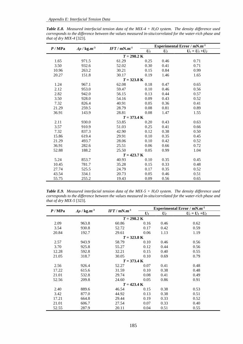
Appendix E: Interfacial Tension Data
185
Table E.8. Measured interfacial tension data of the MIX-4 + H2O system. The density difference used
corresponds to the difference between the values measured in-situ/correlated for the water-rich phase and
that of dry MIX-4 [323].
P / MPa Δρ / kg.m-3 IFT / mN.m-1 Experimental Error / mN.m-1
U1 U2 Uc = U1 +U2
T = 298.2 K
1.65 971.5 61.29 0.25 0.46 0.71
3.50 932.6 52.02 0.30 0.41 0.71
10.96 263.2 30.21 0.15 0.84 0.99
20.27 151.8 30.17 0.19 1.46 1.65
T = 323.8 K
1.24 967.1 62.08 0.18 0.47 0.65
2.12 953.0 59.47 0.10 0.46 0.56
2.82 942.0 56.15 0.13 0.44 0.57
3.50 928.0 54.16 0.09 0.43 0.52
7.32 826.4 40.91 0.05 0.36 0.41
21.29 259.5 28.79 0.08 0.81 0.89
36.91 143.9 28.81 0.08 1.47 1.55
T = 373.4 K
2.11 930.0 53.85 0.20 0.43 0.63
3.57 910.9 51.03 0.25 0.41 0.66
7.32 837.3 42.90 0.12 0.38 0.50
15.86 619.4 29.91 0.10 0.35 0.45
21.29 493.7 28.06 0.10 0.42 0.52
36.91 282.6 25.51 0.06 0.66 0.72
52.88 188.2 25.50 0.05 0.99 1.04
T = 423.7 K
5.24 853.7 40.93 0.10 0.35 0.45
10.45 781.7 35.28 0.15 0.33 0.48
27.74 525.5 24.79 0.17 0.35 0.52
43.54 334.1 20.73 0.05 0.46 0.51
55.75 255.2 19.43 0.09 0.56 0.65
Table E.9. Measured interfacial tension data of the MIX-5 + H2O system. The density difference used
corresponds to the difference between the values measured in-situ/correlated for the water-rich phase and
that of dry MIX-5 [323].
P / MPa Δρ / kg.m-3 IFT / mN.m-1 Experimental Error / mN.m-1
U1 U2 Uc = U1 +U2
T = 298.2 K
2.09 963.8 60.86 0.16 0.46 0.62
3.54 930.8 52.72 0.17 0.42 0.59
20.84 192.7 29.61 0.06 1.13 1.19
T = 323.8 K
2.57 943.9 58.79 0.10 0.46 0.56
3.70 925.8 55.27 0.12 0.44 0.56
12.28 592.8 32.21 0.15 0.40 0.55
21.05 318.7 30.05 0.10 0.69 0.79
T = 373.4 K
2.56 926.4 52.27 0.07 0.41 0.48
17.22 615.6 31.59 0.10 0.38 0.48
21.01 532.8 29.74 0.08 0.41 0.49
52.56 209.8 24.60 0.05 0.86 0.91
T = 423.4 K
2.40 889.6 46.54 0.15 0.38 0.53
3.42 877.0 44.92 0.13 0.38 0.51
17.21 664.8 29.44 0.19 0.33 0.52
21.01 606.7 27.54 0.07 0.33 0.40
52.55 287.9 20.11 0.04 0.51 0.55
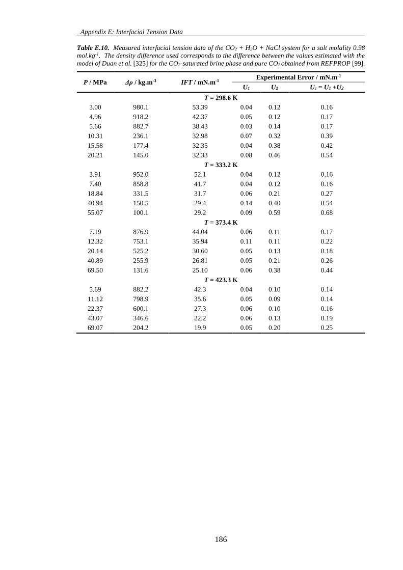
Appendix E: Interfacial Tension Data
186
Table E.10. Measured interfacial tension data of the CO2 + H2O + NaCl system for a salt molality 0.98
mol.kg-1. The density difference used corresponds to the difference between the values estimated with the
model of Duan et al. [325] for the CO2-saturated brine phase and pure CO2 obtained from REFPROP [99].
P / MPa Δρ / kg.m-3 IFT / mN.m-1 Experimental Error / mN.m-1
U1 U2 Uc = U1 +U2
T = 298.6 K
3.00 980.1 53.39 0.04 0.12 0.16
4.96 918.2 42.37 0.05 0.12 0.17
5.66 882.7 38.43 0.03 0.14 0.17
10.31 236.1 32.98 0.07 0.32 0.39
15.58 177.4 32.35 0.04 0.38 0.42
20.21 145.0 32.33 0.08 0.46 0.54
T = 333.2 K
3.91 952.0 52.1 0.04 0.12 0.16
7.40 858.8 41.7 0.04 0.12 0.16
18.84 331.5 31.7 0.06 0.21 0.27
40.94 150.5 29.4 0.14 0.40 0.54
55.07 100.1 29.2 0.09 0.59 0.68
T = 373.4 K
7.19 876.9 44.04 0.06 0.11 0.17
12.32 753.1 35.94 0.11 0.11 0.22
20.14 525.2 30.60 0.05 0.13 0.18
40.89 255.9 26.81 0.05 0.21 0.26
69.50 131.6 25.10 0.06 0.38 0.44
T = 423.3 K
5.69 882.2 42.3 0.04 0.10 0.14
11.12 798.9 35.6 0.05 0.09 0.14
22.37 600.1 27.3 0.06 0.10 0.16
43.07 346.6 22.2 0.06 0.13 0.19
69.07 204.2 19.9 0.05 0.20 0.25
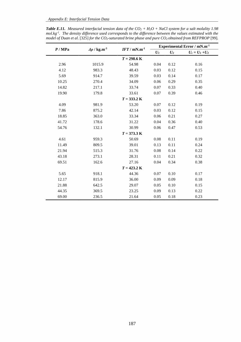
Appendix E: Interfacial Tension Data
187
Table E.11. Measured interfacial tension data of the CO2 + H2O + NaCl system for a salt molality 1.98
mol.kg-1. The density difference used corresponds to the difference between the values estimated with the
model of Duan et al. [325] for the CO2-saturated brine phase and pure CO2 obtained from REFPROP [99].
P / MPa Δρ / kg.m-3 IFT / mN.m-1 Experimental Error / mN.m-1
U1 U2 Uc = U1 +U2
T = 298.6 K
2.96 1015.9 54.98 0.04 0.12 0.16
4.12 983.3 48.43 0.03 0.12 0.15
5.69 914.7 39.59 0.03 0.14 0.17
10.25 270.4 34.09 0.06 0.29 0.35
14.82 217.1 33.74 0.07 0.33 0.40
19.90 179.8 33.61 0.07 0.39 0.46
T = 333.2 K
4.09 981.9 53.20 0.07 0.12 0.19
7.86 875.2 42.14 0.03 0.12 0.15
18.85 363.0 33.34 0.06 0.21 0.27
41.72 178.6 31.22 0.04 0.36 0.40
54.76 132.1 30.99 0.06 0.47 0.53
T = 373.3 K
4.61 959.3 50.69 0.08 0.11 0.19
11.49 809.5 39.01 0.13 0.11 0.24
21.94 515.3 31.76 0.08 0.14 0.22
43.18 273.1 28.31 0.11 0.21 0.32
69.51 162.6 27.16 0.04 0.34 0.38
T = 423.2 K
5.65 918.1 44.36 0.07 0.10 0.17
12.17 815.9 36.00 0.09 0.09 0.18
21.88 642.5 29.07 0.05 0.10 0.15
44.35 369.5 23.25 0.09 0.13 0.22
69.00 236.5 21.64 0.05 0.18 0.23
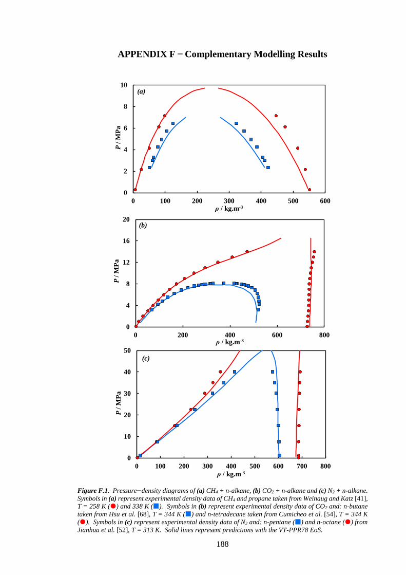
188
APPENDIX F Complementary Modelling Results
Figure F.1. Pressure−density diagrams of (a) CH4 + n-alkane, (b) CO2 + n-alkane and (c) N2 + n-alkane.
Symbols in (a) represent experimental density data of CH4 and propane taken from Weinaug and Katz [41],
T = 258 K () and 338 K (). Symbols in (b) represent experimental density data of CO2 and: n-butane
taken from Hsu et al. [68], T = 344 K () and n-tetradecane taken from Cumicheo et al. [54], T = 344 K
(). Symbols in (c) represent experimental density data of N2 and: n-pentane () and n-octane () from
Jianhua et al. [52], T = 313 K. Solid lines represent predictions with the VT-PPR78 EoS.
0
2
4
6
8
10
0 100 200 300 400 500 600
P /
MP
a
ρ / kg.m-3
0
10
20
30
40
50
0 100 200 300 400 500 600 700 800
P /
MP
a
ρ / kg.m-3
0
4
8
12
16
20
0 200 400 600 800
P /
MP
a
ρ / kg.m-3
(c)
(b)
(a)
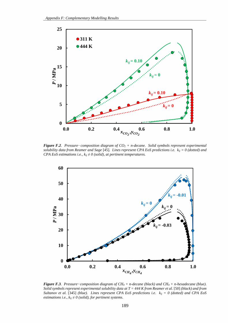
Appendix F: Complementary Modelling Results
189
Figure F.2. Pressure−composition diagram of CO2 + n-decane. Solid symbols represent experimental
solubility data from Reamer and Sage [45]. Lines represent CPA EoS predictions i.e. kij = 0 (dotted) and
CPA EoS estimations i.e., kij ≠ 0 (solid), at pertinent temperatures.
Figure F.3. Pressure−composition diagram of CH4 + n-decane (black) and CH4 + n-hexadecane (blue).
Solid symbols represent experimental solubility data at T = 444 K from Reamer et al. [50] (black) and from
Sultanov et al. [345] (blue). Lines represent CPA EoS predictions i.e. kij = 0 (dotted) and CPA EoS
estimations i.e., kij ≠ 0 (solid), for pertinent systems.
0
5
10
15
20
25
0.0 0.2 0.4 0.6 0.8 1.0
P /
MP
a
xCO2 ,yCO2
311 K
444 K
kij = 0
kij = 0.10
kij = 0.10
kij = 0
0
10
20
30
40
50
60
0.0 0.2 0.4 0.6 0.8 1.0
P /
MP
a
xCH4 ,yCH4
kij = 0
kij = -0.01
kij = -0.03
kij = 0
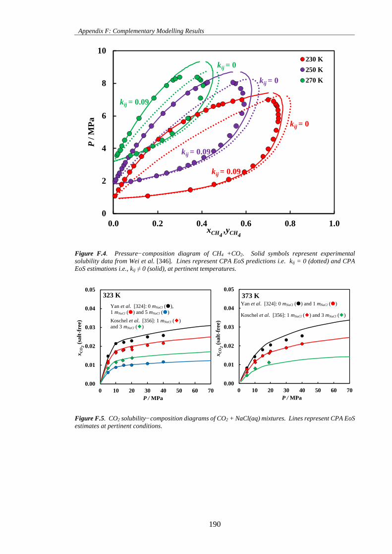
Appendix F: Complementary Modelling Results
190
Figure F.4. Pressure−composition diagram of CH4 +CO2. Solid symbols represent experimental
solubility data from Wei et al. [346]. Lines represent CPA EoS predictions i.e. kij = 0 (dotted) and CPA
EoS estimations i.e., kij ≠ 0 (solid), at pertinent temperatures.
Figure F.5. CO2 solubility−composition diagrams of CO2 + NaCl(aq) mixtures. Lines represent CPA EoS
estimates at pertinent conditions.
0
2
4
6
8
10
0.0 0.2 0.4 0.6 0.8 1.0
P /
MP
a
xCH4 ,yCH4
230 K
250 K
270 K
kij = 0.09
kij = 0
kij = 0
kij = 0
kij = 0.09
kij = 0.09
0.00
0.01
0.02
0.03
0.04
0.05
0 10 20 30 40 50 60 70
xC
O2
(sa
lt-f
ree)
P / MPa
323 K
0.00
0.01
0.02
0.03
0.04
0.05
0 10 20 30 40 50 60 70
xC
O2
(sa
lt-f
ree)
P / MPa
373 K
Yan et al. [324]: 0 mNaCl (), 1 mNaCl () and 5 mNaCl ()
Koschel et al. [356]: 1 mNaCl () and 3 mNaCl ()
Yan et al. [324]: 0 mNaCl () and 1 mNaCl ()
Koschel et al. [356]: 1 mNaCl () and 3 mNaCl ()
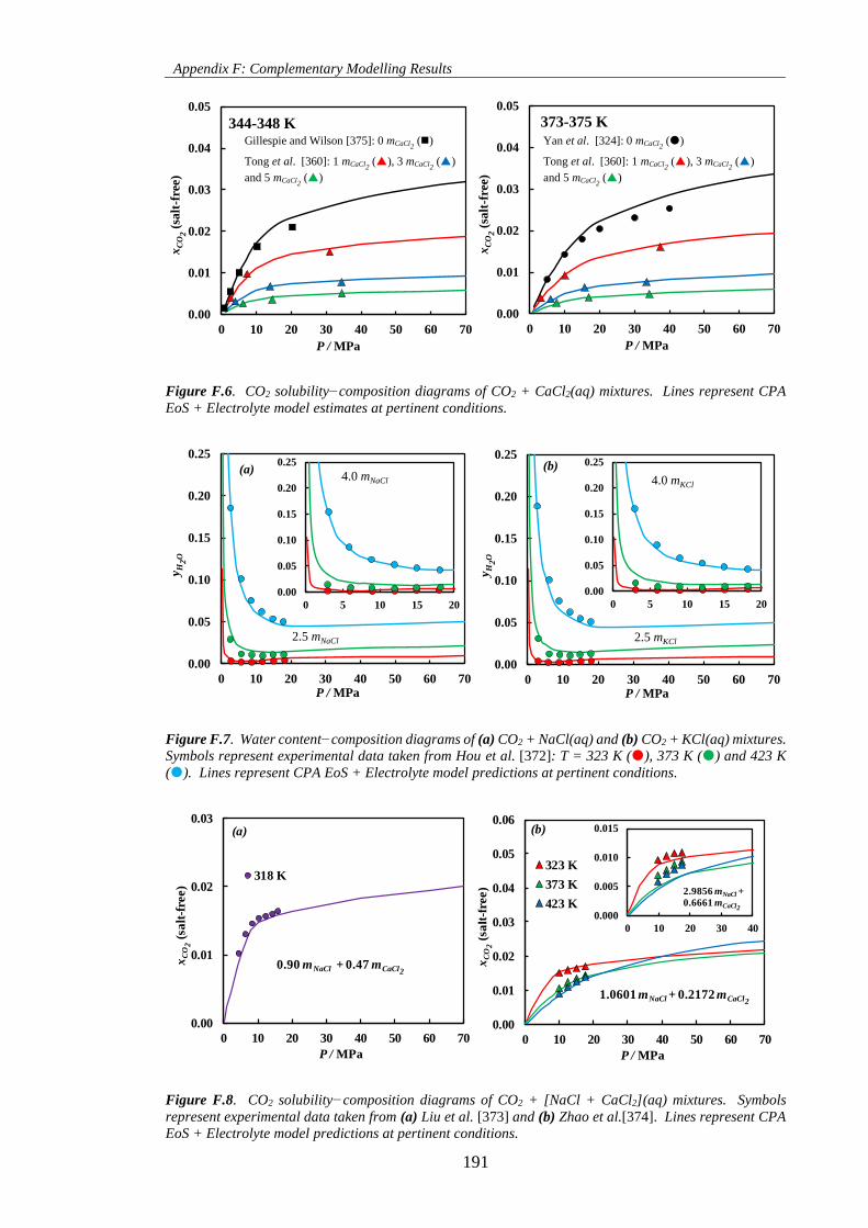
Appendix F: Complementary Modelling Results
191
Figure F.6. CO2 solubility−composition diagrams of CO2 + CaCl2(aq) mixtures. Lines represent CPA
EoS + Electrolyte model estimates at pertinent conditions.
Figure F.7. Water content−composition diagrams of (a) CO2 + NaCl(aq) and (b) CO2 + KCl(aq) mixtures.
Symbols represent experimental data taken from Hou et al. [372]: T = 323 K (), 373 K () and 423 K
(). Lines represent CPA EoS + Electrolyte model predictions at pertinent conditions.
Figure F.8. CO2 solubility−composition diagrams of CO2 + [NaCl + CaCl2](aq) mixtures. Symbols
represent experimental data taken from (a) Liu et al. [373] and (b) Zhao et al.[374]. Lines represent CPA
EoS + Electrolyte model predictions at pertinent conditions.
0.00
0.01
0.02
0.03
0.04
0.05
0 10 20 30 40 50 60 70
xC
O2
(sa
lt-f
ree)
P / MPa
344-348 K
0.00
0.01
0.02
0.03
0.04
0.05
0 10 20 30 40 50 60 70
xC
O2
(sa
lt-f
ree)
P / MPa
373-375 K
0.00
0.05
0.10
0.15
0.20
0.25
0 10 20 30 40 50 60 70
y H2
O
P / MPa
0.00
0.05
0.10
0.15
0.20
0.25
0 5 10 15 20
0.00
0.05
0.10
0.15
0.20
0.25
0 10 20 30 40 50 60 70
y H2O
P / MPa
0.00
0.05
0.10
0.15
0.20
0.25
0 5 10 15 20
4.0 mNaCl
2.5 mNaCl
4.0 mKCl
2.5 mKCl
(a) (b)
0.00
0.01
0.02
0.03
0.04
0.05
0.06
0 10 20 30 40 50 60 70
xC
O2
(sa
lt-f
ree)
P / MPa
323 K
373 K
423 K0.000
0.005
0.010
0.015
0 10 20 30 40
1.0601 mNaCl + 0.2172 mCaCl2
0.00
0.01
0.02
0.03
0 10 20 30 40 50 60 70
xC
O2
(sa
lt-f
ree)
P / MPa
318 K
0.90 mNaCl + 0.47 mCaCl2
(a) (b)
2.9856 mNaCl +
0.6661 mCaCl2
Gillespie and Wilson [375]: 0 mCaCl2 ()
Tong et al. [360]: 1 mCaCl2 (), 3 mCaCl2
()
and 5 mCaCl2 ()
Yan et al. [324]: 0 mCaCl2 ()
Tong et al. [360]: 1 mCaCl2 (), 3 mCaCl2
()
and 5 mCaCl2 ()
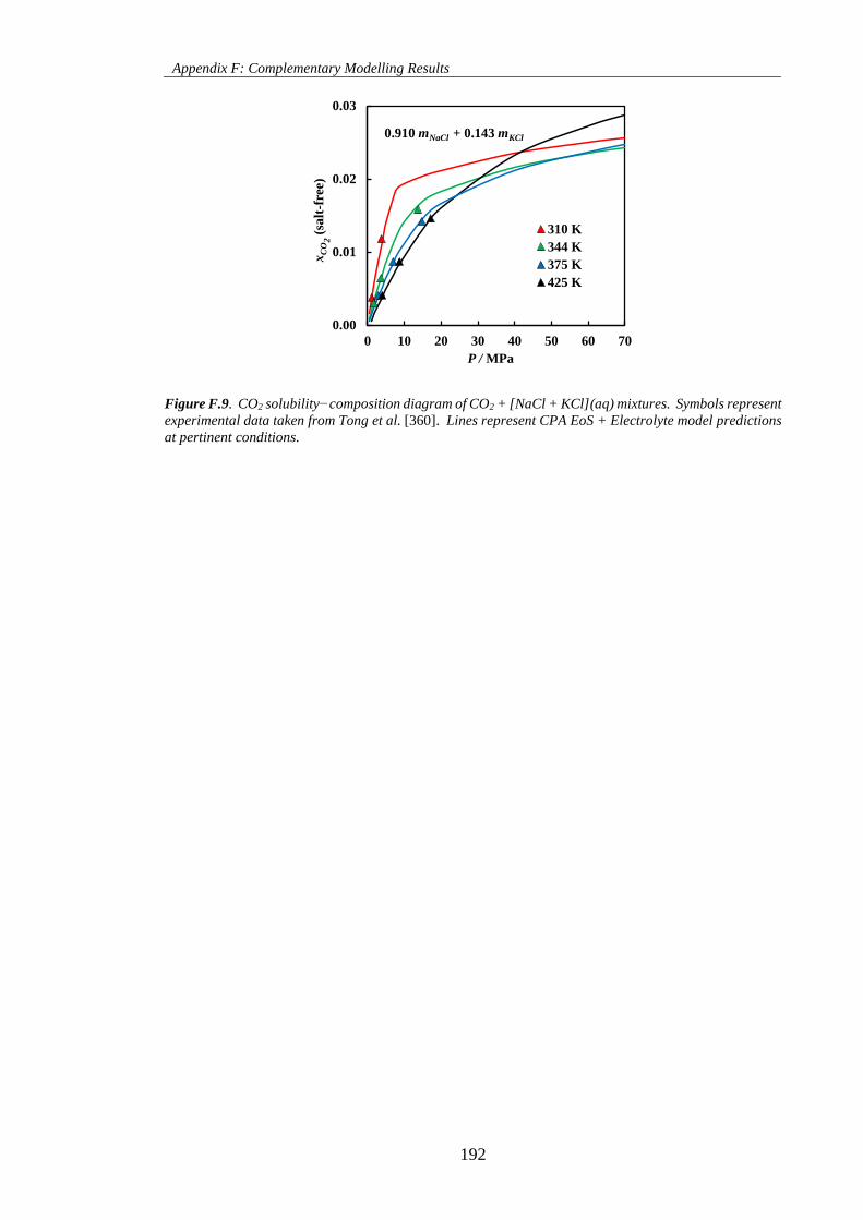
Appendix F: Complementary Modelling Results
192
Figure F.9. CO2 solubility−composition diagram of CO2 + [NaCl + KCl](aq) mixtures. Symbols represent
experimental data taken from Tong et al. [360]. Lines represent CPA EoS + Electrolyte model predictions
at pertinent conditions.
0.00
0.01
0.02
0.03
0 10 20 30 40 50 60 70
xC
O2
(sa
lt-f
ree)
P / MPa
310 K
344 K
375 K
425 K
0.910 mNaCl + 0.143 mKCl
193
REFERENCES
[1] S. Pacala, R. Socolow, Stabilization wedges: solving the climate problem for the
next 50 years with current technologies., Science. 305, 968–72 (2004).
[2] S.J. Altman, B. Aminzadeh, M.T. Balhoff, P.C. Bennett, S.L. Bryant, M.B.
Cardenas, K. Chaudhary, R.T. Cygan, W. Deng, T. Dewers, D.A. DiCarlo, P.
Eichhubl, M.A. Hesse, C. Huh, E.N. Matteo, Y. Mehmani, C.M. Tenney, H. Yoon,
Chemical and hydrodynamic mechanisms for long-term geological carbon
storage, J. Phys. Chem. C. 118, 15103–15113 (2014).
[3] D.W. Green, G.P. Willhite, Enhanced oil recovery, SPE Textbook Series (1998).
[4] J.R. Christensen, E.H. Stenby, A. Skauge, Review of WAG field experience, SPE
Reserv. Eval. Eng. 4, 97–106 (2001).
[5] S.H. Talebian, R. Masoudi, I.M. Tan, P.L.J. Zitha, Foam assisted CO2-EOR: A
review of concept, challenges, and future prospects, J. Pet. Sci. Eng. 120, 202–215
(2014).
[6] A.Y. Dandekar, Petroleum reservoir rock and fluid properties, CRC Press Taylor
& Francis Group (2006).
[7] P. Chiquet, J.-L. Daridon, D. Broseta, S. Thibeau, CO2/water interfacial tensions
under pressure and temperature conditions of CO2 geological storage, Energy
Convers. Manag. 48, 736–744 (2007).
[8] N.K. Adam, The physics and chemistry of surfaces, Third ed., Oxford University
Press (1941).
[9] H.Y. Erbil, Surface chemistry of solid and liquid interfaces, Blackwell Publishing
(2006).
[10] J. Pellicer, J.A. Manzanares, S. Mafé, The physical description of elementary
surface phenomena: Thermodynamics versus mechanics, Am. J. Phys. 63, 542
(1995).
[11] A.I. Rusanov, V.A. Prokhorov, Interfacial tensiometry, Elsevier (1996).
[12] A.W. Neumann, R. David, Y. Zuo, Applied surface thermodynamics, Second ed.,
CRC Press Taylor & Francis Group (2010).
[13] A.W. Adamson, Physical chemistry of surfaces, Fifth ed., John Wiley & Sons,
Inc. (1990).
[14] K. Holmberg, D.O. Shah, M.J. Schwuger, eds., Handbook of applied surface and
colloid chemistry, Vol 1, John Wiley & Sons, Ltd (2002).
[15] J. Straub, The role of surface tension for two-phase heat and mass transfer in the
absence of gravity, Exp. Therm. Fluid Sci. 9, 253–273 (1994).
[16] J.W. Rose, Surface tension effects and enhancement of condensation heat transfer,
Chem. Eng. Res. Des. 82, 419–429 (2004).
[17] A. Abubakar, Y. Al-Wahaibi, T. Al-Wahaibi, A. Al-Hashmi, A. Al-Ajmi, M.
Eshrati, Effect of low interfacial tension on flow patterns, pressure gradients and
holdups of medium-viscosity oil/water flow in horizontal pipe, Exp. Therm. Fluid
Sci. 68, 58–67 (2015).
[18] F.T. Hokmabadi, H. Bahmanyar, M. Amanabadi, J. Safdari, Dispersed phase
194
holdup and slip velocity of phases in a pulsed packed column in conditions with
and without mass transfer, Can. J. Chem. Eng. 87, 855–861 (2009).
[19] W.R. Foster, A low-tension waterflooding process, J. Pet. Technol. 25, 205–210
(1973).
[20] E.J. Lefebvre du Prey, Factors affecting liquid-liquid relative permeabilities of a
consolidated porous medium, Soc. Pet. Eng. J. 13, 39–47 (1973).
[21] R. Ehrlich, H.H. Hasiba, P. Raimondi, Alkaline waterflooding for wettability
alteration-evaluating a potential field application, J. Pet. Technol. 26, 1335–1343
(1974).
[22] J.C. Melrose, Role of capillary forces in detennining microscopic displacement
efficiency for oil recovery by waterflooding, J. Can. Pet. Technol. 13, (1974).
[23] A. Abrams, The influence of fluid viscosity, interfacial tension, and flow velocity
on residual oil saturation left by waterflood, Soc. Pet. Eng. J. 15, 437–447 (1975).
[24] S.G. Oh, J.C. Slattery, Interfacial tension required for significant displacement of
residual oil, Soc. Pet. Eng. J. 19, 83–96 (1979).
[25] S. Zhang, G.-C. Jiang, L. Wang, H.-T. Guo, X. Tang, D.-G. Bai, Foam flooding
with ultra-low interfacial tension to enhance heavy oil recovery, J. Dispers. Sci.
Technol. 35, 403–410 (2014).
[26] O.R. Wagner, R.O. Leach, Effect of interfacial tension on displacement efficiency,
Soc. Pet. Eng. J. 6, (1966).
[27] A. Firoozabadi, D.L. Katz, H. Soroosh, V.A. Sajjadian, Surface tension of
reservoir crude-oil/gas systems recognizing the asphalt in the heavy fraction, SPE
Reserv. Eng. 3, 265–272 (1988).
[28] C. Bardon, D.G. Longeron, Influence of very low interfacial tensions on relative
permeability, Soc. Pet. Eng. J. 391–401 (1980).
[29] M.S. Haniff, J.K. Ali, Relative permeability and low tension fluid flow in gas
condensate systems, in: Proc. Eur. Pet. Conf., Society of Petroleum Engineers
(1990).
[30] J.K. Ali, S. Butler, L. Allen, P. Wardle, The influence of interfacial tension on
liquid mobility in gas condensate systems, in: Offshore Eur., Society of Petroleum
Engineers (1993).
[31] A. Georgiadis, G. Maitland, J.P.M. Trusler, A. Bismarck, Interfacial tension
measurements of the (H2O + n-Decane + CO2) ternary system at elevated
pressures and temperatures, J. Chem. Eng. Data. 56, 4900–4908 (2011).
[32] Z. Li, M. Dong, S. Li, S. Huang, CO2 sequestration in depleted oil and gas
reservoirs—caprock characterization and storage capacity, Energy Convers.
Manag. 47, 1372–1382 (2006).
[33] V. Shah, D. Broseta, G. Mouronval, F. Montel, Water/acid gas interfacial tensions
and their impact on acid gas geological storage, Int. J. Greenh. Gas Control. 2,
594–604 (2008).
[34] S. Iglauer, C.H. Pentland, A. Busch, CO2 wettability of seal and reservoir rocks
and the implications for carbon geo-sequestration, Water Resour. Res. 51, 729–
774 (2015).
[35] E.W. Hough, G.L. Stegemeier, Correlation of surface and interfacial tension of
light hydrocarbons in the critical region, Soc. Pet. Eng. J. 1, 259–263 (1961).
195
[36] S.J.O. Connor, Hydrocarbon-water interfacial tension values at reservoir
conditions: Inconsistencies in the technical literature and the impact on maximum
oil and gas column height calculations, Am. Assoc. Pet. Geol. Bull. 84, 1537–1541
(2000).
[37] S. Krevor, M.J. Blunt, S.M. Benson, C.H. Pentland, C. Reynolds, A. Al-Menhali,
B. Niu, Capillary trapping for geologic carbon dioxide storage – From pore scale
physics to field scale implications, Int. J. Greenh. Gas Control. 40, 221–237 (2015).
[38] S. Bachu, D. Bonijoly, J. Bradshaw, R. Burruss, S. Holloway, N.P. Christensen,
O.M. Mathiassen, CO2 storage capacity estimation: Methodology and gaps, Int. J.
Greenh. Gas Control. 1, 430–443 (2007).
[39] S. Bachu, Sequestration of CO2 in geological media: criteria and approach for
site selection in response to climate change, Energy Convers. Manag. 41, 953–970
(2000).
[40] D.A. Voormeij, G.J. Simandl, Geological, ocean, and mineral CO2 sequestration
options: A technical review, Geosci. Canada. 31, (2004).
[41] C.F. Weinaug, D.L. Katz, Surface tensions of methane-propane mixtures, Ind.
Eng. Chem. 35, 239–246 (1943).
[42] D. Macleod, On a relation between surface tension and density, Trans. Faraday
Soc. 2, 2–5 (1923).
[43] S. Sugden, VI.—The variation of surface tension with temperature and some
related functions, J. Chem. Soc. Trans. 32–41 (1924).
[44] H. Nourozieh, M. Kariznovi, J. Abedi, Measurements and predictions of density
and carbon dioxide solubility in binary mixtures of ethanol and n-decane, J. Chem.
Thermodyn. 58, 377–384 (2013).
[45] H.H. Reamer, B.H. Sage, Phase equilibria in hydrocarbon systems. Volumetric
and phase behavior of the n-Decane-CO2 system., J. Chem. Eng. Data. 8, 508–513
(1963).
[46] N. Nagarajan, R.L. Robinson, Equilibrium phase compositions, phase densities,
and interfacial tensions for carbon dioxide + hydrocarbon systems. 2. Carbon
dioxide + n-decane, J. Chem. Eng. Data. 31, 168–171 (1986).
[47] R.D. Shaver, R.L. Robinson, K.A.M. Gasem, An automated apparatus for
equilibrium phase compositions, densities, and interfacial tensions: data for
carbon dioxide + decane, Fluid Phase Equilib. 179, 43–66 (2001).
[48] A. Mejía, M. Cartes, H. Segura, E.A. Müller, Use of equations of state and coarse
grained simulations to complement experiments: describing the interfacial
properties of carbon dioxide + decane and carbon dioxide + eicosane mixtures, J.
Chem. Eng. Data. 59, 2928–2941 (2014).
[49] B.H. Sage, H.M. Lavender, W.N. Lacey, Phase equilibria in hydrocarbon systems
methane–decane system, Ind. Eng. Chem. 32, 743–747 (1940).
[50] H.H. Reamer, R.H. Olds, B.H. Sage, W.N. Lacey, Phase equilibria in
hydrocarbon systems: methane-decane system, Ind. Eng. Chem. 34, 1526–1531
(1942).
[51] R. Amin, T.N. Smith, Interfacial tension and spreading coefficient under
reservoir conditions, Fluid Phase Equilib. 142, 231–241 (1998).
[52] T. Jianhua, J. Satherley, D.J. Schiffrin, Density and interfacial tension of nitrogen-
196
hydrocarbon systems at elevated pressures, Chin.J.Chem.Eng. 1, 223–231 (1993).
[53] A. Georgiadis, F. Llovell, A. Bismarck, F.J. Blas, A. Galindo, G.C. Maitland,
J.P.M. Trusler, G. Jackson, Interfacial tension measurements and modelling of
(carbon dioxide+n-alkane) and (carbon dioxide+water) binary mixtures at
elevated pressures and temperatures, J. Supercrit. Fluids. 55, 743–754 (2010).
[54] C. Cumicheo, M. Cartes, H. Segura, E.A. Müller, A. Mejía, High-pressure
densities and interfacial tensions of binary systems containing carbon dioxide+n-
alkanes: (n-Dodecane, n-tridecane, n-tetradecane), Fluid Phase Equilib. 380, 82–
92 (2014).
[55] A.S. Danesh, A.Y. Dandekar, A.C. Todd, R. Sarkar, A modified scaling law and
parachor method approach for improved prediction of interfacial tension of gas-
condensate systems, in: SPE Annu. Tech. Conf. Exhib., Society of Petroleum
Engineers (1991).
[56] K. Gasem, B. Kenneth, R. Shaver, R. Robert L., Experimental phase densities and
interfacial tensions for a CO2/synthetic-oil and a CO2/reservoir-oil system, SPE
Reserv. Eng. 8, (1993).
[57] R.J.M. Huygens, H. Ronde, J. Hagoort, Interfacial tension of nitrogen/volatile oil
systems, SPE J. 1, 125–132 (1996).
[58] V.G. Baidakov, A.M. Kaverin, M.N. Khotienkova, Surface tension of ethane–
methane solutions: 1. Experiment and thermodynamic analysis of the results, Fluid
Phase Equilib. 356, 90–95 (2013).
[59] B.F. Pennington, E.W. Hough, Interfacial tension of the methane-normale butane,
Prod. Mon. July, 4 (1965).
[60] R. Massoudi, A.D. King, Effect of pressure on the surface tension of n-hexane.
Adsorption of low molecular weight gases on n-hexane at 25 oC., J. Phys. Chem.
79, 1676–1679 (1975).
[61] O.G. Niño-Amezquita, S. Enders, P.T. Jaeger, R. Eggers, Measurement and
prediction of interfacial tension of binary mixtures, Ind. Eng. Chem. Res. 49, 592–
601 (2010).
[62] H.G. Warren, E.W. Hough, Interfacial tension of the methane-normal heptane
system, Soc. Pet. Eng. J. 10, 327–327 (1970).
[63] P.T. Jaeger, M.B. Alotaibi, H.A. Nasr-El-Din, Influence of compressed carbon
dioxide on the capillarity of the gas−crude oil−reservoir water system, J. Chem.
Eng. Data. 55, 5246–5251 (2010).
[64] P.T. Jaeger, R. Eggers, Interfacial properties at elevated pressures in reservoir
systems containing compressed or supercritical carbon dioxide, J. Supercrit.
Fluids. 66, 80–85 (2012).
[65] B. Peng, C. Sun, B. Liu, Q. Zhang, J. Chen, W. Li, G. Chen, Interfacial tension
between methane and octane at elevated pressure at five temperatures from (274.2
to 282.2) K, J. Chem. Eng. Data. 56, 4623–4626 (2011).
[66] J.R. Deam, R.N. Maddox, Interfacial tension in hydrocarbon systems, J. Chem.
Eng. Data. 15, 216–222 (1970).
[67] G. Stegemeier, B. Pennington, E.B. Brauer, E.W. Hough, Interfacial tension of
the methane-normal decane system, Soc. Pet. Eng. J. 2, 257–260 (1962).
[68] J.J.C. Hsu, N. Nagarajan, R.L. Robinson, Equilibrium phase compositions, phase
197
densities, and interfacial tensions for carbon dioxide + hydrocarbon systems. 1.
Carbon dioxide + n-butane, J. Chem. Eng. Data. 30, 485–491 (1985).
[69] O.G. Niño Amézquita, S. Enders, P.T. Jaeger, R. Eggers, Interfacial properties of
mixtures containing supercritical gases, J. Supercrit. Fluids. 55, 724–734 (2010).
[70] A. Zolghadr, M. Escrochi, S. Ayatollahi, Temperature and composition effect on
CO2 miscibility by interfacial tension measurement, J. Chem. Eng. Data. 58, 1168–
1175 (2013).
[71] K.A.M. Gasem, K.B. Dickson, P.B. Dulcamara, N. Nagarajan, R.L. Robinson,
Equilibrium phase compositions, phase densities, and interfacial-tensions for CO2
+ hydrocarbon systems .5. CO2 + n- tetradecane, J. Chem. Eng. Data. 34, 191–
195 (1989).
[72] V.G. Baidakov, A.M. Kaverin, M.N. Khotienkova, V.N. Andbaeva, Surface
tension of an ethane–nitrogen solution. 1: Experiment and thermodynamic
analysis of the results, Fluid Phase Equilib. 328, 13–20 (2012).
[73] G.J. Reno, D.L. Katz, Surface tension of n-heptane and n-butane containing
dissolved nitrogen, Ind. Eng. Chem. 35, 1091–1093 (1943).
[74] J.M. Garrido, L. Cifuentes, M. Cartes, H. Segura, A. Mejía, High-pressure
interfacial tensions for nitrogen + ethanol, or hexane or 2-methoxy-2-
methylbutane. A comparison between experimental tensiometry and Monte Carlo
simulations, J. Supercrit. Fluids. (2014).
[75] A. Zolghadr, M. Riazi, M. Escrochi, S. Ayatollahi, Investigating the effects of
temperature, pressure, and paraffin groups on the N2 miscibility in hydrocarbon
liquids using the interfacial tension measurement method, Ind. Eng. Chem. Res.
52, 9851–9857 (2013).
[76] E.W. Hough, G.J. Heuer, J.W. Walker, An improved pendant drop, interfacial
tension apparatus and data for carbon dioxide and water, Pet. Trans. AIME. 216,
469–472 (1959).
[77] R. Massoudi, A.D. King, Effect of pressure on the surface tension of water.
Adsorption of low molecular weight gases on water at 25 oC, J. Phys. Chem. 78,
2262–2266 (1974).
[78] C. Jho, D. Nealon, S. Shogbola, A.D. King Jr., Effect of pressure on the surface
tension of water: Adsorption of hydrocarbon gases and carbon dioxide on water
at temperatures between 0 and 50°C, J. Colloid Interface Sci. 65, 141–154 (1978).
[79] B.-S. Chun, G.T. Wilkinson, Interfacial tension in high-pressure carbon dioxide
mixtures, Ind. Eng. Chem. Res. 34, 4371–4377 (1995).
[80] A. Wesch, N. Dahmen, K. Ebert, J. Schön, Grenzflächenspannungen,
Tropfengrößen und Kontaktwinkel im Zweiphasensystem H2O/CO2 bei
Temperaturen von 298 bis 333 K und Drücken bis 30 MPa, Chemie Ing. Tech. 69,
942–946 (1997).
[81] S.R.P. da Rocha, K.L. Harrison, K.P. Johnston, Effect of surfactants on the
interfacial tension and emulsion formation between water and carbon dioxide,
Langmuir. 15, 419–428 (1999).
[82] A. Hebach, A. Oberhof, N. Dahmen, A. Kögel, H. Ederer, E. Dinjus, Interfacial
tension at elevated pressures - Measurements and correlations in the water +
carbon dioxide system, J. Chem. Eng. Data. 47, 1540–1546 (2002).
[83] F. Tewes, F. Boury, Thermodynamic and dynamic interfacial properties of binary
198
carbon dioxide−water systems, J. Phys. Chem. B. 108, 2405–2412 (2004).
[84] J.-Y. Park, J.S. Lim, C.H. Yoon, C.H. Lee, K.P. Park, Effect of a fluorinated
sodium bis(2-ethylhexyl) sulfosuccinate (aerosol-OT, AOT) analogue surfactant
on the interfacial tension of CO2 + water and CO2 + Ni-plating solution in near-
and supercritical CO2, J. Chem. Eng. Data. 50, 299–308 (2005).
[85] D. Yang, P. Tontiwachwuthikul, Y. Gu, Interfacial interactions between reservoir
brine and CO2 at high pressures and elevated temperatures, Energy & Fuels. 19,
216–223 (2005).
[86] T. Akutsu, Y. Yamaji, H. Yamaguchi, M. Watanabe, R.L. Smith, H. Inomata,
Interfacial tension between water and high pressure CO2 in the presence of
hydrocarbon surfactants, Fluid Phase Equilib. 257, 163–168 (2007).
[87] B. Kvamme, T. Kuznetsova, A. Hebach, A. Oberhof, E. Lunde, Measurements
and modelling of interfacial tension for water+carbon dioxide systems at elevated
pressures, Comput. Mater. Sci. 38, 506–513 (2007).
[88] Y. Sutjiadi-Sia, P. Jaeger, R. Eggers, Interfacial phenomena of aqueous systems
in dense carbon dioxide, J. Supercrit. Fluids. 46, 272–279 (2008).
[89] S. Bachu, D.B. Bennion, Interfacial tension between CO2 , freshwater, and brine
in the range of pressure from (2 to 27) MPa, temperature from (20 to 125) °C, and
water salinity from (0 to 334 000) mg·L −1, J. Chem. Eng. Data. 54, 765–775
(2009).
[90] C. Chalbaud, M. Robin, J.-M. Lombard, F. Martin, P. Egermann, H. Bertin,
Interfacial tension measurements and wettability evaluation for geological CO2
storage, Adv. Water Resour. 32, 98–109 (2009).
[91] A. Georgiadis, G. Maitland, J.P.M. Trusler, A. Bismarck, Interfacial tension
measurements of the (H2O + CO2) system at elevated pressures and temperatures,
J. Chem. Eng. Data. 55, 4168–4175 (2010).
[92] P.K. Bikkina, O. Shoham, R. Uppaluri, Equilibrated interfacial tension data of
the CO2-water system at high pressures and moderate temperatures, J. Chem. Eng.
Data. 56, 3725–3733 (2011).
[93] A. Shariat, R.G. Moore, S.A. Mehta, K.C. Van Fraassen, K.E. Newsham, J.A.
Rushing, Laboratory measurements of CO2-H2O interfacial tension at HP/HT
conditions: Implications for CO2 sequestration in deep aquifers, in: Carbon
Manag. Technol. Conf., Carbon Management Technology Conference (2012).
[94] M. Sarmadivaleh, A.Z. Al-Yaseri, S. Iglauer, Influence of temperature and
pressure on quartz–water–CO2 contact angle and CO2–water interfacial tension,
J. Colloid Interface Sci. 441, 59–64 (2015).
[95] R. Yaginuma, Y. Sato, D. Kodama, Saturated densities of carbon dioxide+ water
mixture at 304.1 K and pressures to 10 MPa, Nthon Enerugi Galhzislti. 79, 144–
146 (2000).
[96] A. Hebach, A. Oberhof, N. Dahmen, Density of water + carbon dioxide at
elevated pressures: Measurements and correlation, J. Chem. Eng. Data. 49, 950–
953 (2004).
[97] F. Tabasinejad, Y. Barzin, R.G. Moore, S.A. Mehta, K.C. Van Fraassen, J.
Rushing, K.E. Newsham, Water/CO2 system at high pressure and temperature
conditions: Measurement and modeling of density in equilibrium liquid and vapor
phases, in: SPE Eur. Annu. Conf. Exhib., Society of Petroleum Engineers (2010).
199
[98] E.C. Efika, R. Hoballah, X. Li, E.F. May, M. Nania, Y. Sanchez-Vicente, J.P.
Martin Trusler, Saturated phase densities of (CO2+H2O) at temperatures from
(293 to 450) K and pressures up to 64 MPa, J. Chem. Thermodyn. 93, 347–359
(2016).
[99] E.W. Lemmon, M.O. McLinden, M.L. Huber, NIST Reference Fluid
Thermodynamic and Transport Properties — REFPROP, Version 8.0, NIST,
Gaithersburg, MD, (2007).
[100] G. Wiegand, E.U. Franck, Interfacial tension between water and non-polar fluids
up to 473 K and 2800 bar., Berichte der Bunsengesellschaft für Phys. Chemie. 98,
809–817 (1994).
[101] B.-Y. Cai, J.-T. Yang, T.-M. Guo, Interfacial tension of hydrocarbon +
water/brine systems under high pressure, J. Chem. Eng. Data. 41, 493–496 (1996).
[102] G.Y. Zhao, W. Yan, G.J. Chen, X.Q. Guo, Measurement and calculation of high-
pressure interfacial tension of methane+ nitrogen/water system, Shiyou Daxue
Xuebao/Journal Univ. Pet. China. 26, 75–78+82 (2002).
[103] K. Kashefi, L.M.C. Pereira, A. Chapoy, R. Burgass, B. Tohidi, Measurement and
modelling of interfacial tension in methane/water and methane/brine systems at
reservoir conditions, Fluid Phase Equilib. 409, 301–311 (2016).
[104] Y. Tian, Y. Xiao, H. Zhu, X. Dong, Interfacial tensions between water and non-
polar fluids at high pressures and high temperatures, Acta Physico-Chimica Sin.
13, 89–95 (1997).
[105] Q.Y. Ren, G.J. Chen, W. Yan, T.M. Guo, Interfacial tension of (CO2+CH4) plus
water from 298 K to 373 K and pressures up to 30 MPa, J. Chem. Eng. Data. 45,
610–612 (2000).
[106] W. Yan, G.-Y. Zhao, G.-J. Chen, T.-M. Guo, Interfacial tension of (methane +
nitrogen) + water and (carbon dioxide + nitrogen) + water systems, J. Chem. Eng.
Data. 46, 1544–1548 (2001).
[107] J. Ralston, T.W. Healy, Specific cation effects on water structure at the air-water
and air-octadecanol monolayer-water interfaces, J. Colloid Interface Sci. 42, 629–
644 (1973).
[108] K. Johansson, J.C. Eriksson, Γ and dγ/dT measurements on aqueous solutions of
1,1-electrolytes, J. Colloid Interface Sci. 49, 469–480 (1974).
[109] P.K. Weissenborn, R.J. Pugh, Surface tension of aqueous solutions of electrolytes:
relationship with ion hydration, oxygen solubility, and bubble coalescence, J.
Colloid Interface Sci. 184, 550–563 (1996).
[110] L.M. Pegram, M.T. Record, Hofmeister salt effects on surface tension arise from
partitioning of anions and cations between bulk water and the air−water interface,
J. Phys. Chem. B. 111, 5411–5417 (2007).
[111] Y. Levin, A.P. dos Santos, A. Diehl, Ions at the air-water interface: An end to a
hundred-year-old mystery?, Phys. Rev. Lett. 103, 257802 (2009).
[112] Y. Marcus, Effect of ions on the structure of water: structure making and
breaking., Chem. Rev. 109, 1346–70 (2009).
[113] C. Duchateau, D. Broseta, A simple method for determining brine–gas interfacial
tensions, Adv. Water Resour. 42, 30–36 (2012).
[114] M.J. Hey, D.W. Shield, J.M. Speight, M.C. Will, Surface tensions of aqueous
200
solutions of some 1:1 electrolytes, J. Chem. Soc. Faraday Trans. 1 Phys. Chem.
Condens. Phases. 77, 123 (1981).
[115] X. Li, E. Boek, G.C. Maitland, J.P.M. Trusler, Interfacial tension of (brines +
CO2): (0.864 NaCl + 0.136 KCl) at yemperatures between (298 and 448) K,
pressures between (2 and 50) MPa, and total molalities of (1 to 5) mol·kg -1, J.
Chem. Eng. Data. 57, 1078–1088 (2012).
[116] M.J. Argaud, Predicting the interfacial tension of brine/gas (or condensates)
systems, in: 3rd Eur. Core Anal. Symp., Society of Core Analysts (1992).
[117] X. Li, D.A. Ross, J.P.M. Trusler, G.C. Maitland, E.S. Boek, Molecular dynamics
simulations of CO2 and brine interfacial tension at high temperatures and
pressures., J. Phys. Chem. B. 117, 5647–52 (2013).
[118] L.M.C. Pereira, A. Chapoy, R. Burgass, M.B. Oliveira, J.A.P. Coutinho, B.
Tohidi, Study of the impact of high temperatures and pressures on the equilibrium
densities and interfacial tension of the carbon dioxide/water system, J. Chem.
Thermodyn. 93, 404–415 (2016).
[119] X. Li, E.S. Boek, G.C. Maitland, J.P.M. Trusler, Interfacial tension of (brines +
CO2): CaCl2 (aq), MgCl2 (aq), and NaCl2SO4 (aq) at temperatures between (343
and 423) K, pressures between (2 and 50) MPa, and molalities of (0.5 to 5) mol/kg,
J. Chem. Eng. Data. 57, 1369–1375 (2012).
[120] A. Badakhshan, P. Bakes, The influence of temperature and surfactant
concentration on interfacial tension of saline water and hydrocarbon systems in
relation to enhanced oil recovery by chemical flooding, Soc. Pet. Eng. (1990).
[121] N. Ikeda, M. Aratono, K. Motomura, Thermodynamic study on the adsorption of
sodium chloride at the water/hexane interface, J. Colloid Interface Sci. 149, 208–
215 (1992).
[122] J.A. Rushing, K.E. Newsham, K.C. Van Fraassen, S.A. Mehta, G.R. Moore,
Laboratory measurements of gas-water interfacial tension at HP/HT reservoir
conditions, in: CIPC/SPE Gas Technol. Symp. 2008 Jt. Conf., Society of
Petroleum Engineers (2008).
[123] H.Y. Jennings, G.H. Newman, The effect of temperature and pressure on the
interfacial tension of water against methane-normal decane mixtures, Soc. Pet.
Eng. J. 11, 171–175 (1971).
[124] Reservoir Fluid Studies: 2002-2005 Programme, Final Report, Heriot-Watt
University .
[125] A. Bahramian, A. Danesh, F. Gozalpour, B. Tohidi, A.C. Todd, Vapour–liquid
interfacial tension of water and hydrocarbon mixture at high pressure and high
temperature conditions, Fluid Phase Equilib. 252, 66–73 (2007).
[126] L.M.C. Pereira, A. Chapoy, B. Tohidi, Vapor-liquid and liquid-liquid interfacial
tension of water and hydrocarbon systems at representative reservoir conditions:
Experimental and modelling results, in: SPE Annu. Tech. Conf. Exhib., Society of
Petroleum Engineers (2014).
[127] R. Massoudi, A.D. King, Effect of pressure on the surface tension of aqueous
solutions. Adsorption of hydrocarbon gases, carbon dioxide, and nitrous oxide on
aqueous solutions of sodium chloride and tetrabutylammonium bromide at 25 oC.,
J. Phys. Chem. 79, 1670–1675 (1975).
[128] Y. Liu, M. Mutailipu, L. Jiang, J. Zhao, Y. Song, L. Chen, Interfacial tension and
201
contact angle measurements for the evaluation of CO2-brine two-phase flow
characteristics in porous media, Environ. Prog. Sustain. Energy. 34, 1756–1762
(2015).
[129] C.A. Aggelopoulos, M. Robin, E. Perfetti, O. Vizika, CO2/CaCl2 solution
interfacial tensions under CO2 geological storage conditions: Influence of cation
valence on interfacial tension, Adv. Water Resour. 33, 691–697 (2010).
[130] C.A. Aggelopoulos, M. Robin, O. Vizika, Interfacial tension between CO2 and
brine (NaCl+CaCl2) at elevated pressures and temperatures: The additive effect
of different salts, Adv. Water Resour. 34, 505–511 (2011).
[131] N.E. Dorsey, Measurement of surface tension, Sci. Pap. Bur. Stand. 21, 524–546
(1926).
[132] J. Drelich, C. Fang, C.L. White, Measurement of interfacial tension in fluid-fluid
systems, Encycl. Surf. Colloid Sci. 3152–3166 (2002).
[133] J.D. Berry, M.J. Neeson, R.R. Dagastine, D.Y.C. Chan, R.F. Tabor, Measurement
of surface and interfacial tension using pendant drop tensiometry, J. Colloid
Interface Sci. 454, 226–237 (2015).
[134] J.F. Padday, Surface tension. Part I. The theory of surface tension, in: E. Matijević
(Ed.), Surf. Colloid Surface, Vol . 1, Wiley-Interscience (1969).
[135] U. Henriksson, J.C. Eriksson, Thermodynamics of capillary rise: Why is the
meniscus curved?, J. Chem. Educ. 81, 150 (2004).
[136] M.Á. Rodríguez-Valverde, M. Tirado Miranda, Derivation of Jurin’s law
revisited, Eur. J. Phys. 32, 49–54 (2011).
[137] J.B.T. McCaughan, Capillarity-a lesson in the epistemology of physics, Phys.
Educ. 22, 100–106 (1987).
[138] P.C. Hiemenz, R. Rajagopalan, Principles of colloid and surface chemistry, Third
ed., Marcel Dekker, Inc. (1997).
[139] G.C. Vorlicek, J.W. Warren, G.E. Kilby, Capillarity revisited - yet again, Phys.
Educ. 23, 7–8 (1988).
[140] J.B.T. McCaughan, Capillarity reply, Phys. Educ. 23, 205–206 (1988).
[141] E.K. Chapin, Two contrasting theories of capillary action, Am. J. Phys. 27, 617
(1959).
[142] C.W. Extrand, S.I. Moon, Which controls wetting? Contact line versus interfacial
area: Simple experiments on capillary rise, Langmuir. 28, 15629–15633 (2012).
[143] L. Rayleigh, On the theory of the capillary tube, Proc. R. Soc. A Math. Phys. Eng.
Sci. 92, 184–195 (1916).
[144] G.S. Barozzi, D. Angeli, A note on capillary rise in tubes, Energy Procedia. 45,
548–557 (2014).
[145] S. Sugden, XCVII.—The determination of surface tension from the maximum
pressure in bubbles, J. Chem. Soc., Trans. 121, 858–866 (1922).
[146] J. Lane, Correction terms for calculating surface tension from capillary rise, J.
Colloid Interface Sci. 42, 145–149 (1973).
[147] S. Ramakrishnan, S. Hartland, The determination of interfacial tension by
differential capillary rise, J. Chem. Sci. 90, 215–224 (1981).
[148] H.L. Gielen, O.B. Verbeke, J. Thoen, The critical behavior of the Sugden

202
parameter and the surface tension of simple fluids, J. Chem. Phys. 81, 6154 (1984).
[149] V.A.M. Soares, B. de J.V.S. Almeida, I.A. McLure, R.A. Higgins, Surface tension
of pure and mixed simple substances at low temperatures, Fluid Phase Equilib. 32,
9–16 (1986).
[150] V.A.M. Soares, I.A. McLure, B.S. Almeida, R.A. Higgins, J.C.G. Calado, Cell for
orthobaric surface tension measurements at low temperatures, Cryogenics
(Guildf). 27, 263–265 (1987).
[151] K.C. Nadler, J.A. Zollweg, W.B. Streett, I.A. McLure, Surface tension of argon +
krypton from 120 to 200 K, J. Colloid Interface Sci. 122, 530–536 (1988).
[152] S.B.R. Karri, V.K. Mathur, Measurement of interfacial tension of immiscible
liquids of equal density, AIChE J. 34, 155–157 (1988).
[153] B.A. Grigoryev, B. V. Nemzer, D.S. Kurumov, J. V. Sengers, Surface tension of
normal pentane, hexane, heptane, and octane, Int. J. Thermophys. 13, 453–464
(1992).
[154] V.G. Baidakov, A.M. Kaverin, M.N. Khotienkova, Surface tension of ethane–
methane solutions: 1. Experiment and thermodynamic analysis of the results, Fluid
Phase Equilib. 356, 90–95 (2013).
[155] A.M. Worthington, On pendent drops, Proc. R. Soc. London. 32, 362–377 (1881).
[156] F. Bashforth, J.C. Adams, An attempt to test the theories of capillary action: By
comparing the theoretical and measured forms of drops of fluid, Cambridge
University Press (1883).
[157] J.M. Andreas, E.A. Hauser, W.B. Tucker, Boundary tension by pendant drops, J.
Phys. Chem. 42, 1001–1019 (1937).
[158] S. Fordham, On the calculation of surface tension from measurements of pendant
drops, Proc. R. Soc. London. 194, 1–16 (1948).
[159] D.O. Niederhauser, F.E. Bartell, A corrected table for the calculation of boundary
tensions by the pendant drop method, API Research Project 27 .
[160] Y. Rotenberg, L. Boruvka, A.W. Neumann, Determination of surface tension and
contact angle from the shapes of axisymmetric fluid interfaces, J. Colloid Interface
Sci. 93, 169–183 (1983).
[161] P. Cheng, D. Li, L. Boruvka, Y. Rotenberg, A.W. Neumann, Automation of
axisymmetric drop shape analysis for measurements of interfacial tensions and
contact angles, Colloids and Surfaces. 43, 151–167 (1990).
[162] B. Song, J. Springer, Determination of interfacial tension from the profile of a
pendant drop using computer-aided image processing: 1. Theoretical, J. Colloid
Interface Sci. 184, 64–76 (1996).
[163] B. Song, J. Springer, Determination of interfacial tension from the profile of a
pendant drop using computer-aided image processing: 2. Experimental, J. Colloid
Interface Sci. 184, 77–91 (1996).
[164] M. Hoorfar, a W Neumann, Recent progress in axisymmetric drop shape analysis
(ADSA)., Adv. Colloid Interface Sci. 121, 25–49 (2006).
[165] J.K. Spelt, Y. Rotenberg, D.R. Absolom, A.W. Neumann, Sessile-drop contact
angle measurements using axisymmetric drop shape analysis, Colloids and
Surfaces. 24, 127–137 (1987).
203
[166] O. Río, A. Neumann, Axisymmetric drop shape analysis: Computational methods
for the measurement of interfacial properties from the shape and dimensions of
pendant and sessile drops., J. Colloid Interface Sci. 196, 136–147 (1997).
[167] A. Kalantarian, R. David, A.W. Neumann, Methodology for high accuracy contact
angle measurement, Langmuir. 25, 14146–14154 (2009).
[168] Y.T.F. Chow, D.K. Eriksen, A. Galindo, A.J. Haslam, G. Jackson, G.C. Maitland,
J.P.M. Trusler, Interfacial tensions of systems comprising water, carbon dioxide
and diluent gases at high pressures: Experimental measurements and modelling
with SAFT-VR Mie and square-gradient theory, Fluid Phase Equilib. 407, 159–176
(2016).
[169] Y.T.F. Chow, G.C. Maitland, J.P.M. Trusler, Interfacial tensions of the
(CO2+N2+H2O) system at temperatures of (298 to 448) K and pressures up to 40
MPa, J. Chem. Thermodyn. 93, 392–403 (2016).
[170] S.S. Susnar, H.A. Hamza, A.W. Neumann, Pressure dependence of interfacial
tension of hydrocarbon—water systems using axisymmetric drop shape analysis,
Colloids Surfaces A Physicochem. Eng. Asp. 89, 169–180 (1994).
[171] S.-T. Lee, M. Chien, A new multicomponent surface tension correlation based on
scaling theory, in: SPE Enhanc. Oil Recover. Symp., Society of Petroleum
Engineers (1984).
[172] E.A. Guggenheim, The principle of corresponding states, J. Chem. Phys. 13, 253
(1945).
[173] Y.-X. Zuo, E.H. Stenby, Corresponding-states and parachor models for the
calculation of interfacial tensions, Can. J. Chem. Eng. 75, 1130–1137 (1997).
[174] A.J. Queimada, L.I. Rolo, A.I. Caço, I.M. Marrucho, E.H. Stenby, J.A.P.
Coutinho, Prediction of viscosities and surface tensions of fuels using a new
corresponding states model, Fuel. 85, 874–877 (2006).
[175] L.A. Girifalco, R.J. Good, A theory for the estimation of surface and interfacial
energies. I. Derivation and application to interfacial tension, J. Phys. Chem. 61,
904–909 (1957).
[176] P.H. Winterfield, L.E. Scriven, H.T. Davis, An approximate theory of interfacial
tensions of multicomponent systems : Applications to binary liquid-vapour
tensions, AIChE J. 24, 1010–1014 (1978).
[177] R.P. Sutton, General engineering, Vol. 1, in: J.R. Fanchi, L.W. Lake (Eds.), Pet.
Eng. Handb., Society of Petroleum Engineers (2006): pp. 257–331.
[178] R.P. Sutton, An improved model for water-hydrocarbon surface tension at
reservoir conditions, in: SPE Annu. Tech. Conf. Exhib., Society of Petroleum
Engineers (2009).
[179] A. Danesh, PVT and phase behaviour of petroleum reservoir fluids, Elsevier
Publishing (1998).
[180] A. Firoozabadi, H.J. Ramey, Surface tension of water-hydrocarbon systems at
reservoir conditions, J. Can. Pet. Technol. 27, (1988).
[181] S. Nordholm, M. Johnson, B. Freasier, Generalized van der Waals theory. III. The
prediction of hard sphere structure, Aust. J. Chem. 33, 2139 (1980).
[182] R. Evans, The nature of the liquid-vapour interface and other topics in the
statistical mechanics of non-uniform, classical fluids, Adv. Phys. 28, 143–200
204
(1979).
[183] B.S. Almeida, M.M. Telo da Gama, Surface tension of simple mixtures:
comparison between theory and experiment, J. Phys. Chem. 93, 4132–4138 (1989).
[184] V. Bongiorno, H.T. Davis, Modified Van der Waals theory of fluid interfaces,
Phys. Rev. A. 12, 2213–2224 (1975).
[185] Y.-X. Zuo, E.H. Stenby, Calculation of surface tensions of polar mixtures with a
simplified gradient theory model, J. Chem. Eng. Japan. 29, 159–165 (1996).
[186] Y.-X. Zuo, E.H. Stenby, A linear gradient theory model for calculating interfacial
tensions of mixtures, J. Colloid Interface Sci. 182, 126–132 (1996).
[187] J.W. Cahn, J.E. Hilliard, Free energy of a nonuniform system. I. Interfacial free
energy, J. Chem. Phys. 28, 258 (1958).
[188] J.S. Rowlinson, Translation of J. D. van der Waals’ The thermodynamik theory of
capillarity under the hypothesis of a continuous variation of density, J. Stat. Phys.
20, 197–200 (1979).
[189] B.S. Carey, L.E. Scriven, H.T. Davis, Semiempirical theory of surface tensions of
pure normal alkanes and alcohols, AIChE J. 24, 1076–1080 (1978).
[190] Y.-X. Zuo, E.H. Stenby, Calculation of interfacial tensions with gradient theory,
Fluid Phase Equilib. 132, 139–158 (1997).
[191] C. Miqueu, B. Mendiboure, A. Graciaa, J. Lachaise, Modelling of the surface
tension of pure components with the gradient theory of fluid interfaces: a simple
and accurate expression for the influence parameters, Fluid Phase Equilib. 207,
225–246 (2003).
[192] C. Miqueu, B. Mendiboure, C. Graciaa, J. Lachaise, Modelling of the surface
tension of binary and ternary mixtures with the gradient theory of fluid interfaces,
Fluid Phase Equilib. 218, 189–203 (2004).
[193] A. Mejía, I. Polishuk, H. Segura, J. Wisniak, Estimation of interfacial behavior
using the global phase diagram approach I. Carbon dioxide–n-alkanes,
Thermochim. Acta. 411, 171–176 (2004).
[194] C. Miqueu, B. Mendiboure, A. Graciaa, J. Lachaise, Modeling of the surface
tension of multicomponent mixtures with the gradient theory of fluid interfaces,
Ind. Eng. Chem. Res. 44, 3321–3329 (2005).
[195] A.J. Queimada, C. Miqueu, I.M. Marrucho, G.M. Kontogeorgis, J.A.P. Coutinho,
Modeling vapor–liquid interfaces with the gradient theory in combination with the
CPA equation of state, Fluid Phase Equilib. 228-229, 479–485 (2005).
[196] C. Miqueu, B. Mendiboure, A. Graciaa, J. Lachaise, Petroleum mixtures: An
efficient predictive method for surface tension estimations at reservoir conditions,
Fuel. 87, 612–621 (2008).
[197] E.A. Müller, A. Mejía, Interfacial properties of selected binary mixtures
containing n-alkanes, Fluid Phase Equilib. 282, 68–81 (2009).
[198] O. Vilaseca, L.F. Vega, Direct calculation of interfacial properties of fluids close
to the critical region by a molecular-based equation of state, Fluid Phase Equilib.
306, 4–14 (2011).
[199] B. Breure, C.J. Peters, Modeling of the surface tension of pure components and
mixtures using the density gradient theory combined with a theoretically derived
influence parameter correlation, Fluid Phase Equilib. 334, 189–196 (2012).
205
[200] E. Schäfer, G. Sadowski, S. Enders, Interfacial tension of binary mixtures
exhibiting azeotropic behavior: Measurement and modeling with PCP-SAFT
combined with Density Gradient Theory, Fluid Phase Equilib. 362, 151–162
(2014).
[201] P.M.W. Cornelisse, M. Wijtkamp, C.J. Peters, J. de Swaan Arons, Interfacial
tensions of fluid mixtures with polar and associating components, Fluid Phase
Equilib. 150-151, 633–640 (1998).
[202] H. Kahl, S. Enders, Calculation of surface properties of pure fluids using density
gradient theory and SAFT-EOS, Fluid Phase Equilib. 172, 27–42 (2000).
[203] D. Fu, Investigation of surface tensions for pure associating fluids by perturbed-
chain statistical associating fluid Theory combined with density-gradient theory,
Ind. Eng. Chem. Res. 46, 7378–7383 (2007).
[204] M.B. Oliveira, I.M. Marrucho, J.A.P. Coutinho, A.J. Queimada, Surface tension
of chain molecules through a combination of the gradient theory with the CPA
EoS, Fluid Phase Equilib. 267, 83–91 (2008).
[205] M.B. Oliveira, J.A.P. Coutinho, A.J. Queimada, Surface tensions of esters from a
combination of the gradient theory with the CPA EoS, Fluid Phase Equilib. 303,
56–61 (2011).
[206] S.V.D. Freitas, M.B. Oliveira, A.J. Queimada, M.J. Pratas, Á.S. Lima, J.A.P.
Coutinho, Measurement and prediction of biodiesel surface tensions, Energy &
Fuels. 25, 4811–4817 (2011).
[207] S. Enders, K. Quitzsch, Calculation of interfacial properties of demixed fluids
using density gradient theory, Langmuir. 14, 4606–4614 (1998).
[208] C.I. Poser, I.C. Sanchez, Surface tension theory of pure liquids and polymer melts,
J. Colloid Interface Sci. 69, 539–548 (1979).
[209] G.T. Dee, B.B. Sauer, The molecular weight and temperature dependence of
polymer surface tension: Comparison of experiment with interface gradient theory,
J. Colloid Interface Sci. 152, 85–103 (1992).
[210] B.B. Sauer, G.T. Dee, Studies of polymer, copolymer, and associating liquids by
melt surface tension methods and Cahn-Hilliard density-gradient theory, J.
Colloid Interface Sci. 162, 25–35 (1994).
[211] S. Fisk, Structure and free energy of the interface between fluid phases in
equilibrium near the critical point, J. Chem. Phys. 50, 3219 (1969).
[212] A.J.M. Yang, P.D. Fleming III, J.H. Gibbs, Molecular theory of surface tension,
J. Chem. Phys. 64, 3732 (1976).
[213] M.K. Gupta, R.L. Robinson Jr., Application of gradient theory of inhomogeneous
fluid to prediction of low interfacial tensions in CO2/hydrocarbon systems, SPE
Reserv. Eng. 528–530 (1987).
[214] M. Sahimi, B.N. Taylor, Surface tension of binary liquid–vapor mixtures: A
comparison of mean-field and scaling theories, J. Chem. Phys. 95, 6749 (1991).
[215] H. Nilssen, A. Fredheim, E. Solbraa, B. Kvamme, Theoretical prediction of
interfacial tensions for hydrocarbon mixtures with gradient theory in combination
with Peng-Robinson equation of state, in: Proc. Offshore Technol. Conf., Society
of Petroleum Engineers (2010).
[216] X.-S. Li, J.-M. Liu, D. Fu, Investigation of interfacial tensions for carbon dioxide
206
aqueous solutions by perturbed-chain statistical associating fluid theory combined
with density-gradient theory, Ind. Eng. Chem. Res. 47, 8911–8917 (2008).
[217] T. Lafitte, B. Mendiboure, M.M. Piñeiro, D. Bessières, C. Miqueu, Interfacial
properties of water/CO2: a comprehensive description through a Gradient Theory-
SAFT-VR Mie approach., J. Phys. Chem. B. 114, 11110–6 (2010).
[218] C. Miqueu, J.M. Míguez, M.M. Piñeiro, T. Lafitte, B. Mendiboure, Simultaneous
application of the gradient theory and Monte Carlo molecular simulation for the
investigation of methane/water interfacial properties., J. Phys. Chem. B. 115,
9618–25 (2011).
[219] G. Niño-Amézquita, D. van Putten, S. Enders, Phase equilibrium and interfacial
properties of water+CO2 mixtures, Fluid Phase Equilib. 332, 40–47 (2012).
[220] S. Khosharay, M. Abolala, F. Varaminian, Modeling the surface tension and
surface properties of (CO2 + H2O) and (H2S + H2O) with gradient theory in
combination with sPC–SAFT EOS and a new proposed influence parameter, J.
Mol. Liq. 198, 292–298 (2014).
[221] S. Khosharay, F. Varaminian, Experimental and modeling investigation on
surface tension and surface properties of (CH4 + H2O), (C2H6 + H2O), (CO2 +
H2O) and (C3H8 + H2O) from 284.15 K to 312.15 K and pressures up to 60 bar,
Int. J. Refrig. 47, 26–35 (2014).
[222] O.G. Niño-Amézquita, S. Enders, Phase equilibrium and interfacial properties of
water+methane mixtures, Fluid Phase Equilib. 407, 143–151 (2016).
[223] J.M. Míguez, J.M. Garrido, F.J. Blas, H. Segura, A. Mejía, M.M. Piñeiro,
Comprehensive characterization of interfacial behavior for the mixture CO2 +
H2O + CH4 : Comparison between atomistic and coarse grained molecular
simulation models and density gradient theory, J. Phys. Chem. C. 118, 24504–
24519 (2014).
[224] L.C. Nielsen, I.C. Bourg, G. Sposito, Predicting CO2 –water interfacial tension
under pressure and temperature conditions of geologic CO2 storage, Geochim.
Cosmochim. Acta. 81, 28–38 (2012).
[225] E.A. Müller, A. Mejía, Resolving discrepancies in the measurements of the
interfacial tension for the CO2 + H2 O mixture by computer simulation, J. Phys.
Chem. Lett. 5, 1267–1271 (2014).
[226] S. Iglauer, M.S. Mathew, F. Bresme, Molecular dynamics computations of brine-
CO2 interfacial tensions and brine-CO2 -quartz contact angles and their effects on
structural and residual trapping mechanisms in carbon geo-sequestration., J.
Colloid Interface Sci. 386, 405–14 (2012).
[227] J. Neyt, A. Wender, V. Lachet, P. Malfreyt, Modeling the pressure dependence of
acid gas + n -alkane interfacial tensions using atomistic monte carlo simulations.,
J. Phys. Chem. C. 116, 10563–10572 (2012).
[228] O. Lobanova, A. Mejía, G. Jackson, E.A. Müller, SAFT-γ force field for the
simulation of molecular fluids 6: Binary and ternary mixtures comprising water,
carbon dioxide, and n-alkanes, J. Chem. Thermodyn. 93, 320–336 (2016).
[229] B. Liu, J. Shi, M. Wang, J. Zhang, B. Sun, Y. Shen, X. Sun, Reduction in
interfacial tension of water–oil interface by supercritical CO2 in enhanced oil
recovery processes studied with molecular dynamics simulation, J. Supercrit.
Fluids. 111, 171–178 (2016).
207
[230] F. Biscay, A. Ghoufi, V. Lachet, P. Malfreyt, Monte Carlo calculation of the
methane-water interfacial tension at high pressures, J. Chem. Phys. 131, 124707
(2009).
[231] R. Sakamaki, A.K. Sum, T. Narumi, R. Ohmura, K. Yasuoka, Thermodynamic
properties of methane/water interface predicted by molecular dynamics
simulations., J. Chem. Phys. 134, 144702 (2011).
[232] G. Javanbakht, M. Sedghi, W. Welch, L. Goual, Molecular Dynamics Simulations
of CO2/Water/Quartz Interfacial Properties: Impact of CO2 Dissolution in Water.,
Langmuir. 31, 5812–9 (2015).
[233] Y. Liu, T. Lafitte, A.Z. Panagiotopoulos, P.G. Debenedetti, Simulations of vapor-
liquid phase equilibrium and interfacial tension in the CO2-H2O-NaCl system,
AIChE J. 59, 3514–3522 (2013).
[234] G. Soave, Equilibrium constants from a modified Redlich-Kwong equation of
state, Chem. Eng. Sci. 27, 1197–1203 (1972).
[235] D.B. Robinson, D.-Y. Peng, The characterization of the heptanes and heavier
fractions for the GPA Peng-Robinson programs, Gas Processors Association,
Research Report RR-28, (1978).
[236] W.G. Chapman, K.E. Gubbins, G. Jackson, M. Radosz, SAFT: Equation-of-state
solution model for associating fluids, Fluid Phase Equilib. 52, 31–38 (1989).
[237] W.G. Chapman, K.E. Gubbins, G. Jackson, M. Radosz, New reference equation
of state for associating liquids, Ind. Eng. Chem. Res. 29, 1709–1721 (1990).
[238] S.H. Huang, M. Radosz, Equation of state for small, large, polydisperse, and
associating molecules, Ind. Eng. Chem. Res. 29, 2284–2294 (1990).
[239] G.M. Kontogeorgis, M.L. Michelsen, G.K. Folas, S. Derawi, N. von Solms, E.H.
Stenby, Ten years with the CPA (cubic-plus-association) equation of state. Part 1.
Pure compounds and self-associating systems, Ind. Eng. Chem. Res. 45, 4855–
4868 (2006).
[240] G.M. Kontogeorgis, M.L. Michelsen, G.K. Folas, S. Derawi, N. von Solms, E.H.
Stenby, Ten years with the CPA (cubic-plus-association) equation of state. Part 2.
Cross-associating and multicomponent systems, Ind. Eng. Chem. Res. 45, 4869–
4878 (2006).
[241] J. Ali, Prediction of parachors of petroleum cuts and pseudocomponents, Fluid
Phase Equilib. 95, 383–398 (1994).
[242] D. Broseta, Y. Meleán, C. Miqueu, Parachors of liquid/vapor systems: a set of
critical amplitudes, Fluid Phase Equilib. 233, 86–95 (2005).
[243] J.R. Fanchi, Calculation of parachors for compositional simulation: An update,
SPE Reserv. Eng. 5, 433–436 (1990).
[244] M.J. Fawcett, Evaluation of correlations and parachors to predict low interfacial
tensions in condensate systems, in: SPE Annu. Tech. Conf. Exhib., Society of
Petroleum Engineers (1994).
[245] C. Miqueu, J. Satherley, B. Mendiboure, J. Lachaise, A. Graciaa, The effect of
P/N/A distribution on the parachors of petroleum fractions, Fluid Phase Equilib.
180, 327–344 (2001).
[246] J.D. van der Waals, Thermodynamische Theorie der Kapillarität unter
Voraussetzung stetiger Dichteänderung, Z. Phys. Chem. 13, 657–725 (1894).
208
[247] V. Bongiorno, L.E. Scriven, H.T. Davis, Molecular theory of fluid interfaces, J.
Colloid Interface Sci. 57, 462–475 (1976).
[248] H.T. Davis, Statistical mechanics of phases, interfaces and thin films, Wiley
(1995).
[249] B.S. Carey, The gradient theory of fluid interfaces (PhD thesis), University of
Minnesota, USA (1979).
[250] P.M.W. Cornelisse, The square gradient theory applied: Simultaneous modelling
of interfacial tension and phase behaviour (PhD thesis), Delft University of
Technology, The Netherlands (1997).
[251] B.F. McCoy, H.T. Davis, Free-energy theory of inhomogeneous fluids, Phys. Rev.
A. 20, 1201–1207 (1979).
[252] B.S. Carey, L.E. Scriven, H.T. Davis, Semiempirical theory of surface tension of
binary systems, AIChE J. 26, 705–711 (1980).
[253] H.T. Davis, L.E. Scriven, Stress and structure in fluid interfaces, in: Adv. Chem.
Phys., (1982): pp. 357–454.
[254] C. Miqueu, Modélisation à température et pression élevées de la tension
superficielle de composants des fluides pétroliers et de leurs mélanges synthétiques
ou réels (PhD thesis), Université de Pau et des Pays de l’Adour, France (2001).
[255] J.S. Rowlinson, B. Widom, Molecular theory of capillarity, Claredon Press:
Oxford, U.K. (1982).
[256] H. Lin, Y.-Y. Duan, Q. Min, Gradient theory modeling of surface tension for pure
fluids and binary mixtures, Fluid Phase Equilib. 254, 75–90 (2007).
[257] A. Peneloux, E. Rauzy, R. Freze, A consistent correction for Redlich-Kwong-
Soave volumes, Fluid Phase Equilib. 8, 7–23 (1982).
[258] S. Khosharay, M.S. Mazraeno, F. Varaminian, Modeling the surface tension of
refrigerant mixtures with linear gradient theory, Int. J. Refrig. 36, 2223–2232
(2013).
[259] DIPPR 801, Themophysical Properties Database, (1998).
[260] J.M.H.L. Sengers, Mean-field theories, their weaknesses and strength, Fluid
Phase Equilib. 158-160, 3–17 (1999).
[261] A. Mejía, Comportamiento interfacial de mezclas fluidas en equilibrio (PhD
thesis), Universidad de Concepción, Chile (2004).
[262] B.S. Carey, L.E. Scriven, H.T. Davis, On gradient theories of fluid interfacial
stress and structure, J. Chem. Phys. 69, 5040 (1978).
[263] M. Sahimi, H.T. Davis, L.E. Scriven, Thermodynamic modeling of phase and
tension behavior of CO2/hydrocarbon systems, Soc. Pet. Eng. J. 25, 235–254
(1985).
[264] M.M. Telo da Gama, R. Evans, The structure and surface tension of the liquid-
vapour interface near the upper critical end point of a binary mixture of Lennard-
Jones fluids, Mol. Phys. 48, 229–250 (1983).
[265] T. Wadewitz, J. Winkelmann, Density functional theory: Structure and interfacial
properties of binary mixtures, Berichte der Bunsengesellschaft für Phys. Chemie.
100, 1825–1832 (1996).
[266] Y.-X. Zuo, E.H. Stenby, Prediction of interfacial tensions of reservoir crude oil
209
and gas condensate systems, SPE J. 3, 134–145 (1998).
[267] K.A.G. Schmidt, G.K. Folas, B. Kvamme, Calculation of the interfacial tension
of the methane–water system with the linear gradient theory, Fluid Phase Equilib.
261, 230–237 (2007).
[268] S. Khosharay, F. Varaminian, Modeling interfacial tension of (CH4+N2)+H2O
and (N2+CO2)+H2O systems using linear gradient theory, Korean J. Chem. Eng.
30, 724–732 (2013).
[269] Y.-X. Zuo, E.H. Stenby, Calculation of interfacial tensions of hydrocarbon-water
systems under reservoir conditions, Situ. 22, 157–180 (1998).
[270] M.L. Michelsen, J.M. Mollerup, Thermodynamic models: Fundamentals &
Computational aspects, Second ed., Tie-Line Publications (2007).
[271] J.-N. Jaubert, F. Mutelet, VLE predictions with the Peng–Robinson equation of
state and temperature dependent kij calculated through a group contribution
method, Fluid Phase Equilib. 224, 285–304 (2004).
[272] J.-N. Jaubert, S. Vitu, F. Mutelet, J.-P. Corriou, Extension of the PPR78 model
(predictive 1978, Peng–Robinson EOS with temperature dependent kij calculated
through a group contribution method) to systems containing aromatic compounds,
Fluid Phase Equilib. 237, 193–211 (2005).
[273] F. Mutelet, S. Vitu, R. Privat, J.-N. Jaubert, Solubility of CO2 in branched alkanes
in order to extend the PPR78 model (predictive 1978, Peng–Robinson EOS with
temperature-dependent kij calculated through a group contribution method) to
such systems, Fluid Phase Equilib. 238, 157–168 (2005).
[274] J.-N. Jaubert, R. Privat, F. Mutelet, Predicting the phase equilibria of synthetic
petroleum fluids with the PPR78 approach, AIChE J. 56, 3225–3235 (2010).
[275] J.-W. Qian, J.-N. Jaubert, R. Privat, Prediction of the phase behavior of alkene-
containing binary systems with the PPR78 model, Fluid Phase Equilib. 354, 212–
235 (2013).
[276] X. Xu, R. Privat, J.-N. Jaubert, Addition of the sulfur dioxide group (SO2), the
oxygen Group (O2), and the nitric oxide Group (NO) to the E-PPR78 Model, Ind.
Eng. Chem. Res. 54, 9494–9504 (2015).
[277] X. Xu, J.-N. Jaubert, R. Privat, P. Duchet-Suchaux, F. Braña-Mulero, Predicting
binary-interaction parameters of cubic equations of state for petroleum fluids
containing pseudo-components, Ind. Eng. Chem. Res. 54, 2816–2824 (2015).
[278] J.J. Martin, Cubic equations of state - Which?, Ind. Eng. Chem. Fundam. 18, 81–
97 (1979).
[279] A.M. Abudour, S.A. Mohammad, R.L. Robinson, K.A.M. Gasem, Volume-
translated Peng–Robinson equation of state for saturated and single-phase liquid
densities, Fluid Phase Equilib. 335, 74–87 (2012).
[280] A.M. Abudour, S.A. Mohammad, R.L. Robinson, K.A.M. Gasem, Volume-
translated Peng-Robinson equation of state for liquid densities of diverse binary
mixtures, Fluid Phase Equilib. 349, 37–55 (2013).
[281] I. V. Yakoumis, G.M. Kontogeorgis, E.C. Voutsas, E.M. Hendriks, D.P. Tassios,
Prediction of phase equilibria in binary aqueous systems containing alkanes,
cycloalkanes, and alkenes with the cubic-plus-association equation of state, Ind.
Eng. Chem. Res. 37, 4175–4182 (1998).
210
[282] M.B. Oliveira, J.A.P. Coutinho, A.J. Queimada, Mutual solubilities of
hydrocarbons and water with the CPA EoS, Fluid Phase Equilib. 258, 58–66
(2007).
[283] G.K. Folas, G.M. Kontogeorgis, M.L. Michelsen, E.H. Stenby, Application of the
cubic-plus-association (CPA) equation of state to complex mixtures with aromatic
hydrocarbons, Ind. Eng. Chem. Res. 45, 1527–1538 (2006).
[284] G.K. Folas, J. Gabrielsen, M.L. Michelsen, E.H. Stenby, G.M. Kontogeorgis,
Application of the cubic-plus-association (CPA) equation of state to cross-
associating systems, Ind. Eng. Chem. Res. 44, 3823–3833 (2005).
[285] S.O. Derawi, G.M. Kontogeorgis, M.L. Michelsen, E.H. Stenby, Extension of the
cubic-plus-association equation of state to glycol−water cross-associating
systems, Ind. Eng. Chem. Res. 42, 1470–1477 (2003).
[286] M.P. Breil, G.M. Kontogeorgis, Thermodynamics of triethylene glycol and
tetraethylene glycol containing systems described by the cubic-plus-association
equation of state, Ind. Eng. Chem. Res. 48, 5472–5480 (2009).
[287] M.B. Oliveira, M.G. Freire, I.M. Marrucho, G.M. Kontogeorgis, A.J. Queimada,
J.A.P. Coutinho, Modeling the liquid−liquid equilibria of water + fluorocarbons
with the cubic-plus-association equation of state, Ind. Eng. Chem. Res. 46, 1415–
1420 (2007).
[288] I. Tsivintzelis, G.M. Kontogeorgis, M.L. Michelsen, E.H. Stenby, Modeling phase
equilibria for acid gas mixtures using the CPA equation of state. Part II: Binary
mixtures with CO2, Fluid Phase Equilib. 306, 38–56 (2011).
[289] H. Haghighi, A. Chapoy, B. Tohidi, Methane and water phase equilibria in the
presence of single and mixed electrolyte solutions using the cubic-plus-association
equation of state, Oil Gas Sci. Technol. 64, 141–154 (2009).
[290] F. Tabasinejad, R.G. Moore, S.A. Mehta, K.C. Van Fraassen, Y. Barzin, J.A.
Rushing, K.E. Newsham, Water solubility in supercritical methane, nitrogen, and
carbon dioxide: measurement and modeling from 422 to 483 K and pressures from
3.6 to 134 MPa, Ind. Eng. Chem. Res. 50, 4029–4041 (2011).
[291] P.J. Carvalho, A.R. Ferreira, M.B. Oliveira, M. Besnard, M.I. Cabaco, J.A.P.
Coutinho, High pressure phase behavior of carbon dioxide in carbon disulfide and
carbon tetrachloride, J. Chem. Eng. Data. 56, 2786–2792 (2011).
[292] M.B. Oliveira, A.J. Queimada, G.M. Kontogeorgis, J.A.P. Coutinho, Evaluation
of the CO2 behavior in binary mixtures with alkanes, alcohols, acids and esters
using the Cubic-Plus-Association Equation of State, J. Supercrit. Fluids. 55, 876–
892 (2011).
[293] G.M. Kontogeorgis, I. V Yakoumis, H. Meijer, E. Hendriks, T. Moorwood,
Multicomponent phase equilibrium calculations for water-methanol-alkane
mixtures, Fluid Phase Equilib. 158-160, 201–209 (1999).
[294] E.C. Voutsas, G.C. Boulougouris, I.G. Economou, D.P. Tassios,
Water/hydrocarbon phase equilibria using the thermodynamic perturbation
theory, Ind. Eng. Chem. Res. 39, 797–804 (2000).
[295] J.A. Awan, I. Tsivintzelis, C. Coquelet, G.M. Kontogeorgis, Phase equilibria of
three binary mixtures: Methanethiol + methane, methanethiol + nitrogen, and
methanethiol + carbon dioxide, J. Chem. Eng. Data. 57, 896–901 (2012).
[296] B.N. Taylor, C.E. Kuyatt, Guidelines for evaluating and expressing the
211
uncertainty of NIST measurement results, National Institute of Standards and
Technology (1994).
[297] A. Azarnoosh, J.J. McKetta, Nitrogen-n-decane system in the two-phase region,
J. Chem. Eng. Data. 8, 494–496 (1963).
[298] F. Feyzi, M. Seydi, F. Alavi, Crossover Peng-Robinson equation of state with
introduction of a new expression for the crossover function, Fluid Phase Equilib.
293, 251–260 (2010).
[299] H. Behnejad, H. Cheshmpak, A. Jamali, The extended crossover Peng–Robinson
equation of state for describing the thermodynamic properties of pure fluids, J.
Stat. Phys. 158, 372–385 (2015).
[300] D. Fu, Y. Wei, Investigation of vapor−liquid surface tension for carbon dioxide
and hydrocarbon mixtures by perturbed-chain statistical associating fluid theory
combined with density-gradient theory, Ind. Eng. Chem. Res. 47, 4490–4495
(2008).
[301] Reservoir Fluid Studies: 1990-1993 Programme, Final Report, Heriot-Watt
University, UK .
[302] A.Y. Dandekar, Interfacial tension and viscosity of reservoir fluids (PhD thesis),
Heriot Watt University, UK (1994).
[303] M.R. Riazi, Characterization and properties of petroleum fractions, American
Society for Testing and Materials (2005).
[304] C.H. Whitson, M.R. Brulé, Phase behavior, Society of Petroleum Engineering
Inc. (2000).
[305] M.R. Riazi, T.E. Daubert, Characterization parameters for petroleum fractions,
Ind. Eng. Chem. Res. 26, 755–759 (1987).
[306] W.C. Edmister, Applied hydrocarbon thermodynamics, Part 4: Compressibility
factors and equations of State, Pet. Refin. 37, 173–179 (1958).
[307] B.I. Lee, M.G. Kesler, A generalized thermodynamic correlation based on three-
parameter corresponding states, AIChE J. 21, 510–527 (1975).
[308] M.G. Kesler, B.I. Lee, Improve prediction of enthalpy of fractions, Hydrocarb.
Process. 55, 153–158 (1976).
[309] C.H. Twu, An internally consistent correlation for predicting the critical
properties and molecular weights of petroleum and coal-tar liquids, Fluid Phase
Equilib. 16, 137–150 (1984).
[310] A. Firoozabadi, A. Khalid, Analysis and correlation of nitrogen and lean-gas
miscibility pressure, SPE Reserv. Eng. 1, 575–582 (1986).
[311] H. Doryani, Y. Kazemzadeh, R. Parsaei, M.R. Malayeri, M. Riazi, Impact of
asphaltene and normal paraffins on methane-synthetic oil interfacial tension: An
experimental study, J. Nat. Gas Sci. Eng. 26, 538–548 (2015).
[312] P.M.W. Cornelisse, C.J. Peters, J.D. Arons, Application of the Peng-Robinson
equation of state to calculate interfacial-tensions and profiles at vapor-liquid
interfaces, Fluid Phase Equilib. 82, 119–129 (1993).
[313] P.M.W. Cornelisse, C.J. Peters, J. De Swaan Arons, Simultaneous prediction of
phase equilibria, interfacial tension and concentration profiles, Mol. Phys. 80,
941–955 (1993).
212
[314] M.B. King, A. Mubarak, J.D. Kim, T.R. Bott, The mutual solubilities of water
with supercritical and liquid carbon dioxide, J. Supercrit. Fluids. 5, 296–302
(1992).
[315] L.W. Diamond, N.N. Akinfiev, Solubility of CO2 in water from −1.5 to 100 °C
and from 0.1 to 100 MPa: evaluation of literature data and thermodynamic
modelling, Fluid Phase Equilib. 208, 265–290 (2003).
[316] A. Valtz, A. Chapoy, C. Coquelet, P. Paricaud, D. Richon, Vapour–liquid
equilibria in the carbon dioxide–water system, measurement and modelling from
278.2 to 318.2K, Fluid Phase Equilib. 226, 333–344 (2004).
[317] J.M. Miguez, M.C. dos Ramos, M.M. Pineiro, F.J. Blas, An examination of the
ternary methane + carbon dioxide + water phase diagram using the SAFT-VR
approach, J. Phys. Chem. B. 115, 9604–9617 (2011).
[318] R.L. Scott, P.H. van Konynenburg, Static properties of solutions. Van der Waals
and related models for hydrocarbon mixtures, Discuss. Faraday Soc. 49, 87 (1970).
[319] P.H. V. Konynenburg, R.L. Scott, Critical lines and phase equilibria in binary
van der Waals mixtures, Philos. Trans. R. Soc. A Math. Phys. Eng. Sci. 298, 495–
540 (1980).
[320] Z. Duan, R. Sun, An improved model calculating CO2 solubility in pure water and
aqueous NaCl solutions from 273 to 533 K and from 0 to 2000 bar, Chem. Geol.
193, 257–271 (2003).
[321] S.-X. Hou, G.C. Maitland, J.P.M. Trusler, Measurement and modeling of the
phase behavior of the (carbon dioxide+water) mixture at temperatures from
298.15K to 448.15K, J. Supercrit. Fluids. 73, 87–96 (2013).
[322] A. Chapoy, M. Nazeri, M. Kapateh, R. Burgass, C. Coquelet, B. Tohidi, Effect of
impurities on thermophysical properties and phase behaviour of a CO2-rich system
in CCS, Int. J. Greenh. Gas Control. 19, 92–100 (2013).
[323] M.N. Ghojogh, Impact of impurities on thermo-physical properties of CO2-rich
systems: Experimental and modelling (PhD thesis), Heriot-Watt University, UK
(2015).
[324] W. Yan, S. Huang, E.H. Stenby, Measurement and modeling of CO2 solubility in
NaCl brine and CO2–saturated NaCl brine density, Int. J. Greenh. Gas Control. 5,
1460–1477 (2011).
[325] Z. Duan, J. Hu, D. Li, S. Mao, Densities of the CO2 –H2O and CO2 –H2O–NaCl
systems up to 647 K and 100 MPa, Energy & Fuels. 22, 1666–1674 (2008).
[326] Z. Duan, N. Møller, J.H. Weare, An equation of state for the CH4-CO2-H2O
system: I. Pure systems from 0 to 1000°C and 0 to 8000 bar, Geochim.
Cosmochim. Acta. 56, 2605–2617 (1992).
[327] Z. Duan, R. Sun, C. Zhu, I.-M. Chou, An improved model for the calculation of
CO2 solubility in aqueous solutions containing Na+, K+, Ca2+, Mg2+, Cl-, and SO42-
, Mar. Chem. 98, 131–139 (2006).
[328] J.C. Peiper, K.S. Pitzer, Thermodynamics of aqueous carbonate solutions
including mixtures of sodium carbonate, bicarbonate, and chloride, J. Chem.
Thermodyn. 14, 613–638 (1982).
[329] S. Mao, Z. Duan, A thermodynamic model for calculating nitrogen solubility, gas
phase composition and density of the N2–H2O–NaCl system, Fluid Phase Equilib.
248, 103–114 (2006).
213
[330] G. Bergin, Prévision de la solubilité des hydrocarbures dans l’eau en fonction de
la température et de la pression (PhD thesis), Université Blaise Pascal-Clermont-
Ferrand, France (2002).
[331] IUPAC-NIST Solubility data series. 81. Hydrocarbons with water and seawater—
Revised and updated. Part 4. C6H14 hydrocarbons with water, J. Phys. Chem. Ref.
Data. 34, 709 (2005).
[332] IUPAC-NIST Solubility data series. 81. Hydrocarbons with water and seawater—
Revised and updated. Part 11. C13–C36 hydrocarbons with water, J. Phys. Chem.
Ref. Data. 35, 687 (2006).
[333] IUPAC-NIST Solubility data series. 81. Hydrocarbons with water and seawater—
Revised and updated. Part 9. C10 hydrocarbons with water, J. Phys. Chem. Ref.
Data. 35, 93 (2006).
[334] A. Maczynski, Recommended liquid–liquid equilibrium data. Part 1. Binary
alkane–water Systems, J. Phys. Chem. Ref. Data. 33, 549 (2004).
[335] M. Medeiros, Mutual solubilities of water and hydrocarbons from the Cubic plus
Association equation of state: A new mixing rule for the correlation of observed
minimum hydrocarbon solubilities, Fluid Phase Equilib. 368, 5–13 (2014).
[336] N. Spycher, K. Pruess, J. Ennis-King, CO2-H2O mixtures in the geological
sequestration of CO2. I. Assessment and calculation of mutual solubilities from 12
to 100°C and up to 600 bar, Geochim. Cosmochim. Acta. 67, 3015–3031 (2003).
[337] S. Takenouchi, G.C. Kennedy, The binary system H2O-CO2 at high temperatures
and pressures, Am. J. Sci. 262, 1055–1074 (1964).
[338] A. Chapoy, A.H. Mohammadi, D. Richon, B. Tohidi, Gas solubility measurement
and modeling for methane–water and methane–ethane–n-butane–water systems at
low temperature conditions, Fluid Phase Equilib. 220, 111–119 (2004).
[339] O.L. Culberson, H. A.B., J.J.J. McKetta, Phase equilibria in hydrocarbon-water
systems, Pet. Trans. AIME. 189, 1–6 (1950).
[340] R.G. Sultanov, V.G. Skripka, A.Y. Namiot, Rastvormost Metana V Vode Pri
Novysjennykh Temperaturakh I Davlenijakh, Gaz. Prom. 6–7 (1971).
[341] M. Rigby, J.M. Prausnitz, Solubility of water in compressed nitrogen, argon, and
methane, J. Phys. Chem. 72, 330–334 (1968).
[342] R. Wiebe, V.L. Gaddy, C. Heinss, Solubility of nitrogen in water in at 25oC from
25 to 1000 atmospheres, Ind. Eng. Chem. 24, 927–927 (1932).
[343] T.D. O’Sullivan, N.O. Smith, Solubility and partial molar volume of nitrogen and
methane in water and in aqueous sodium chloride from 50 to 125oC and 100 to
600 atm, J. Phys. Chem. 74, 1460–1466 (1970).
[344] T.S. Khasanshin, V.S. Samuilov, A.P. Shchemelev, Determination of the
thermodynamic properties of liquid n-hexadecane from the measurements of the
velocity of sound, J. Eng. Phys. Thermophys. 82, 149–156 (2009).
[345] R.G. Sultanov, V.G. Skripka, A.Y. Namoit, No Title, Gazov. Delo. 10, (1972).
[346] M.S.-W. Wei, T.S. Brown, A.J. Kidnay, E.D. Sloan, Vapor + liquid equilibria for
the ternary system methane + ethane + carbon dioxide at 230 K and its constituent
binaries at temperatures from 207 to 270 K, J. Chem. Eng. Data. 40, 726–731
(1995).
[347] S.Z.S. Al Ghafri, E. Forte, G.C. Maitland, J.J. Rodriguez-Henríquez, J.P.M.
214
Trusler, Experimental and modeling study of the phase behavior of (methane +
CO2 + water) mixtures., J. Phys. Chem. B. 118, 14461–78 (2014).
[348] E. Forte, A. Galindo, J.P.M. Trusler, Experimental and molecular modeling study
of the three-phase behavior of (n-decane + carbon dioxide + water) at reservoir
conditions, 14591–14609 (2011).
[349] Z. Duan, S. Mao, A thermodynamic model for calculating methane solubility,
density and gas phase composition of methane-bearing aqueous fluids from 273 to
523 K and from 1 to 2000 bar, Geochim. Cosmochim. Acta. 70, 3369–3386 (2006).
[350] K.Y. Song, R. Kobayashi, The water content of a carbon dioxide-rich gas mixture
containing 5.31 mol% methane along the three-phase and supercritical conditions,
J. Chem. Eng. Data. 35, 320–322 (1990).
[351] K. Aasberg-Petersen, E. Stenby, A. Fredenslund, Prediction of high-pressure gas
solubilities in aqueous mixtures of electrolytes, Ind. Eng. Chem. Res. 30, 2180–
2185 (1991).
[352] H. Haghighi, Phase equilibria modelling of petroleum reservoir fluids containing
water, hydrate inhibitors and electrolyte solutions (PhD thesis), Heriot-Watt
University, UK (2009).
[353] V.S. Patwardhan, A. Kumar, A unified approach for prediction of thermodynamic
properties of aqueous mixed-electrolyte solutions. Part I: Vapor pressure and heat
of vaporization, AIChE J. 32, 1419–1428 (1986).
[354] B. Tohidi, Gas hydrate equilibria in the presence of electrolyte solutions (PhD
thesis), Heriot-Watt University, UK (1995).
[355] S. Takenouchi, G.C. Kennedy, The solubility of carbon Dioxide in NaCl solutions
at high temperatures and pressures, Am. J. Sci. 263, 445–454 (1965).
[356] D. Koschel, J.-Y. Coxam, L. Rodier, V. Majer, Enthalpy and solubility data of
CO2 in water and NaCl(aq) at conditions of interest for geological sequestration,
Fluid Phase Equilib. 247, 107–120 (2006).
[357] P.J. Carvalho, L.M.C. Pereira, N.P.F. Gonçalves, A.J. Queimada, J.A.P. Coutinho,
Carbon dioxide solubility in aqueous solutions of NaCl: Measurements and
modeling with electrolyte equations of state, Fluid Phase Equilib. 388, 100–106
(2015).
[358] Á. Pérez-Salado Kamps, E. Meyer, B. Rumpf, G. Maurer, Solubility of CO2 in
Aqueous Solutions of KCl and in Aqueous Solutions of K2CO3, J. Chem. Eng. Data.
52, 817–832 (2007).
[359] H. Zhao, R.M. Dilmore, S.N. Lvov, Experimental studies and modeling of CO2
solubility in high temperature aqueous CaCl2, MgCl2, Na2SO4, and KCl solutions,
AIChE J. 61, 2286–2297 (2015).
[360] D. Tong, J.P.M. Trusler, D. Vega-Maza, Solubility of CO2 in aqueous solutions of
CaCl2 or MgCl2 and in a synthetic formation brine at temperatures up to 423 K
and pressures up to 40 MPa, J. Chem. Eng. Data. 58, 2116–2124 (2013).
[361] C.J. Radke, Gibbs adsorption equation for planar fluid-fluid interfaces: Invariant
formalism., Adv. Colloid Interface Sci. 222, 600–14 (2015).
[362] L.A. Turkevich, J.A. Mann, Pressure dependence of the interfacial tension
between fluid phases. 1. Formalism and application to simple fluids, Langmuir. 6,
445–456 (1990).
215
[363] E. Bertrand, H. Dobbs, D. Broseta, J. Indekeu, D. Bonn, J. Meunier, First-order
and critical wetting of alkanes on water, Phys. Rev. Lett. 85, 1282–5 (2000).
[364] D.R. Babu, V. Hornof, G. Neale, Effects of temperature and time on interfacial
tension behavior between heavy oils and alkaline solutions, Can. J. Chem. Eng.
62, 156–159 (1984).
[365] A.A.S. Al-Rossies, B.D. Al-Anazi, A.M. Paiaman, Effect of pH-values on the
contact angle and interfacial tension, Nafta. 61, 181–186 (2010).
[366] P.M. Larsen, B. Maribo-Mogensen, G.M. Kontogeorgis, A collocation method for
surface tension calculations with the density gradient theory, Fluid Phase Equilib.
408, 170–179 (2015).
[367] J. Kou, S. Sun, An adaptive finite element method for simulating surface tension
with the gradient theory of fluid interfaces, J. Comput. Appl. Math. 255, 593–604
(2014).
[368] J. Kou, S. Sun, X. Wang, Efficient numerical methods for simulating surface
tension of multi-component mixtures with the gradient theory of fluid interfaces,
Comput. Methods Appl. Mech. Eng. 292, 92–106 (2015).
[369] J. Kou, S. Sun, Numerical methods for a multicomponent two-phase interface
model with geometric mean influence parameters, SIAM J. Sci. Comput. 37,
B543–B569 (2015).
[370] X.-H. Xu, Y.-Y. Duan, Crossover CPA equation of state for associating fluids,
Fluid Phase Equilib. 290, 148–152 (2010).
[371] X.-H. Xu, Y.-Y. Duan, Z. Yang, Prediction of the critical properties of binary
alkanol+alkane mixtures using a crossover CPA equation of state, Fluid Phase
Equilib. 309, 168–173 (2011).
[372] S.-X. Hou, G.C. Maitland, J.P.M. Trusler, Phase equilibria of (CO2+H2O+NaCl)
and (CO2+H2O+KCl): Measurements and modeling, J. Supercrit. Fluids. 78, 78–
88 (2013).
[373] Y. Liu, M. Hou, G. Yang, B. Han, Solubility of CO2 in aqueous solutions of NaCl,
KCl, CaCl2 and their mixed salts at different temperatures and pressures, J.
Supercrit. Fluids. 56, 125–129 (2011).
[374] H. Zhao, R. Dilmore, D.E. Allen, S.W. Hedges, Y. Soong, S.N. Lvov,
Measurement and modeling of CO2 solubility in natural and synthetic formation
brines for CO2 sequestration, Environ. Sci. Technol. 49, 1972–80 (2015).
[375] P.C. Gillespie, G.M. Wilson, Vapor-liquid and liquid-liquid equilibria: water-
methane, water-carbon dioxide, water-hydrogen sulfide, water-n-pentane, water-
methane-n-pentane. Gas Processors Assocaition. Tulsa. Research Report RR 48,
(1982).


![Modeling Interfacial Surface Tension in Fluid Flo · Our surface tension model is based on the continuum surface force (CSF) approach of Brackbill et al. [1] in which the interfacial](https://static.fdocuments.in/doc/165x107/5edc886bad6a402d66673b5a/modeling-interfacial-surface-tension-in-fluid-our-surface-tension-model-is-based.jpg)


![Measurement of Surface Interfacial Tension as a Function ...mems.cecs.ucf.edu/papers/2012 Measurement of Surface Interfacial Tension.pdf · Downloaded by [University of Central Florida],](https://static.fdocuments.in/doc/165x107/5d61ad5d88c993d6258be42a/measurement-of-surface-interfacial-tension-as-a-function-memscecsucfedupapers2012.jpg)