Interconnection Guidelines for Distributed...
132
Interconnection Guidelines for Distributed Generation Roger Dugan Robert Zavadil David Van Holde, Project Director August 2002 E SOURCE & Electrotek Concepts
Transcript of Interconnection Guidelines for Distributed...
�
Interconnection Guidelines for Distributed Generation
.6-5*�$-*&/5�456%:�
Roger Dugan
Robert Zavadil
David Van Holde, Project Director
August 2002
E SOURCE & Electrotek Concepts
tbasso
Release to post as per David Van Holde; contact him if you have questions.
This report is published exclusively for subscribers to the E SOURCE/Electrotek
Concepts Multi-Client Study “Interconnection Guidelines for Distributed
Generation.” Study subscribers also have access to a password-protected area on the
E SOURCE Web site (www.esource.com). For additional information about this
report, other Multi-Client Studies, other publications and research activities, or
E SOURCE in general, please contact us at:
1MBUUT�
3333 Walnut Street
Boulder, CO 80301-2515
Tel 720-548-5000
Fax 720-548-5001
E-mail [email protected]
Web www.esource.com
&MFDUSPUFL�$PODFQUT
408 North Cedar Bluff Road, Suite 500
Knoxville, TN 37923
Tel 865-470-9222
Fax 865-470-9223
Web www.electrotek.com
© 2002 Electrotek Concepts Inc. and Platts/The McGraw-Hill Companies, Inc.
Reproduction of this publication in any form is prohibited except with the written
permission of Platts or Electrotek Concepts Inc.
Data and information published in the “Interconnection Guidelines for Distributed
Generation” are published with the intention of being accurate. Neither Platts nor
Electrotek, however, can insure against or be held responsible for inaccuracies and
assumes no liability for any loss whatsoever arising from use of such data and
information.
E SOURCE is a registered trademark of Platts.
Electrotek Concepts is a registered service mark of Electrotek Concepts, Inc.
TABLE OF CONTENTS Acknowledgments i
About the Authors ii
Executive Summary 1
1. Introduction 3
2. Utility Distribution System Design 5
2.1 Steady-State Operation/Voltage Regulation 5
2.2 Overcurrent Protection 7
2.3 Planning and Economics 12
3. DR Interconnection Technologies 20
3.1 DG Models for Power System Studies 20
3.2 Characteristics of DG Interface Technologies: Rotating Machines 21
3.3 Characteristics of DG Interface Technologies: Static Power Converters 30
4. Interconnection Requirements 37
4.1 General Protection Requirements 37
4.2 Protection of the DR/EPS Interface 42
4.3 Effect on Transformer Connections 48
5. Power Quality and Reliability 56
5.1 Voltage Regulation Issues 56
5.2 Impact on Utility Overcurrent Protection 61
5.3 Improving Reliability with DR 67
5.4 Adverse Impacts of DR on Utility Reliability 76
5.5 Harmonics from DR 79
6. Application Problems 82
6.1 Voltage Change upon Interconnection or Reclose After a Fault 82
6.2 Harmonic Surprise with Rotation Machines 84
6.3 Desensitizing Utility Relays 86
6.4 Coordinating with Reclosing 89
6.5 Ferroresonance 90
6.6 Capacitor Switching 94
7. Engineering Analysis of DR Interconnection 97
7.1 Basic Power Flow 97
7.2 Fault Studies 110
7.3 Dynamics 116
7.4 Electromagnetic Transients 122
Notes 125

INTERCONNECTION GUIDELINES FOR DISTRIBUTED GENERATION
Distribution outside sponsoring organization prohibited. ii
Acknowledgments
We would like to thank the following people who provided advice, reviewed the
material, and made other contributions to this study:
Bryan Gernet Arizona Public Service
Ronald Onate Arizona Public Service
Mike Doyle Oncor
Scott Castelaz Encorp
INTERCONNECTION GUIDELINES FOR DISTRIBUTED GENERATION
Distribution outside sponsoring organization prohibited. ii
About the Authors David Van Holde, PE, is director of the E SOURCE Distributed Energy Service. Formerly a Senior Energy Analyst for Seattle City Light, David managed the utility’s commercial and industrial multiresource audit program. He also led the provider’s Distributed Generation Task Force, investigating trends, testing technologies, and making policy recommendations to utility management on DG. Task Force achievements included development and implementation of City Light’s Net Metering Program, participation in a fuel cell pilot, and installation of a microturbine, as well as evaluation of several large photovoltaic installations proposed in Seattle. In addition, David managed utility sponsorship of a major retrofit of Seattle Public Schools’ lighting and fan systems that resulted in savings of more than 17 million kilowatt-hours per year. He has had extensive experience with industrial and commercial energy analysis and engineering, training, and report preparation. David holds a BEME from Pratt Institute and an MS in mechanical engineering from Oregon State University, both with emphasis in energy engineering; his master’s thesis focused on institutional cogeneration.
Roger C. Dugan is a senior consultant for Electrotek Concepts Inc., Knoxville, Tennessee. He has more than 30 years’ experience in the power industry, much of which has been devoted to distribution system analysis. He has been working on issues related to distributed resources (DR) interconnection with utility distribution systems for more than 20 years. In recent years, he has been developing software and training materials for helping utility distribution engineers include DR in the planning process. He is the coauthor of Electric Power Systems Quality (McGraw-Hill) and is a Fellow of the IEEE.
Robert Zavadil is marketing manager and senior consultant for Electrotek Concepts Inc. He has more than 20 years of experience in the power industry, including 13 years with Electrotek and 7 years with Nebraska Public Power District. At Electrotek, he has consulted for a variety of clients in electric power quality, distributed photovoltaic applications, wind energy, and other forms of distributed generation. At Nebraska Public Power District he was a staff engineer in the Protection and Control and Substation Engineering departments and performed technical studies related to transmission and distribution system protection, power quality, and grounding. He is a member of the IEEE.
Editorial services: Gail Reitenbach
INTERCONNECTION GUIDELINES FOR DISTRIBUTED GENERATION
Distribution outside sponsoring organization prohibited. 1
Executive Summary
Most electric distribution systems are designed and operated on the premise of there
being a single source of electrical potential on each distribution feeder at any given
time. Distributed resources (DR) violate this basic assumption. Although most
experts agree that distribution systems can safely accommodate a few modestly sized
DR units, the possible effects of connecting large amounts is a source of major
concern to utility engineers, and many question the value of DR to the utility.
Unfortunately, until this guidebook’s publication, there is a dearth of practical
information for utility engineers to help them understand and deal with DR as it
becomes more common. This guidebook compiles current engineering practice for
assessing and mitigating DR impacts on electrical distribution systems and overviews
some methods used to assess the costs and benefits of interconnection.
A review of the pertinent elements of utility system design, focused on protection,
and distribution planning and economics applied to the costs and benefits of DR in a
distribution system provides background to the rest of this guide. An electrical
engineering overview of the dominant DR technologies as they affect the electrical
power system is provided, followed by common DR interconnection technologies
and interconnection requirements. These are directly related to the Institute of
Electrical and Electronics Engineers Draft Standard for Interconnecting Distributed
Resources with Electric Power Systems (IEEE P1547). These requirements are
explained and expanded with examples of simple and complex DR interface
protection schemes. Effects of various interconnection transformers on the protection
and performance of both the DR and the utility distribution systems are reviewed in
detail.
Power quality and reliability impacts of DR are considered generally and via specific
application examples, with mitigation strategies where DR may negatively impact the
distribution system, as well as applications where DR will support customers or
utilities.
An engineering analysis of DR interconnection completes the guidebook, offering
utility distribution engineers an understanding both of how DR elements can be
incorporated into their common systems analysis toolbox and also when and how
more sophisticated dynamic and transient analysis may be needed.

INTERCONNECTION GUIDELINES FOR DISTRIBUTED GENERATION
Distribution outside sponsoring organization prohibited. 3
1. Introduction
As is frequently pointed out, distributed generation (DG) is not a new idea. The
earliest electric generation equipment was distributed, that is, located very close to
the electric loads designated to use the power they generated. This situation,
however, was of necessity rather than choice, because there was no electric utility
distribution infrastructure to interconnect with. Rapid acceptance of electric energy
begat a booming industry, and the race to build ever-larger generating units and
higher-voltage transmission networks dominated the business of the electric utility
industry for the better part of the 20th century.
As the great leaps in central generating unit size and efficiency began to get smaller
and the oil shocks of the 1970s increased attention on and scrutiny of the electric
energy infrastructure, interest in distributed generation was renewed. This time,
however, it was apparent that the preferred mode of operation for small, modular
electric power sources would be in parallel with the existing electric distribution
system. In this “best of both worlds” scenario, the unique values of DG technology—
such as environmental friendliness, fuel price stability, and transmission and
distribution savings—could be realized without sacrificing the stability and security
of the normal utility supply.
More than two decades of serious research and investigation have gone into
identifying and understanding the myriad technical issues associated with
nonnegligible amounts of generation connected to utility distribution systems. Much
light has been shed on the potential technical impacts that distributed generation can
have on distribution system design, operation, and protection. At the same time, DG
technology has become more sophisticated and capable, giving hope for the eventual
resolution of some of the more difficult integration aspects. At the core, however, the
fundamental technical problem remains the same: A vast proportion of the installed
electrical distribution plant in the U.S. was designed and is operated on the
presumption of a single source of electric potential at any instant in time. Distributed
generation obviously violates that premise and, at some capacity level, will
influence—degrade under many circumstances—the reliability, performance, and
possibly safety of any utility distribution feeder.
The popularity of the concept of using distributed generation for electric power
systems of the future increased substantially in the latter part of the 1990s. Growing
awareness at the public policy level has become a major driver. This most recent
groundswell is leading to mandates for streamlining the evaluation process for
approval to interconnect distributed generation with the utility distribution system.
Such policy shifts are happening in spite of the fact that much of what has been
INTERCONNECTION GUIDELINES FOR DISTRIBUTED GENERATION
Distribution outside sponsoring organization prohibited. 4
learned technically about DG’s effects on the distribution system has not been
validated with field experience and has yet to make its way into conventional
distribution system engineering practice.
Work to establish a common technical understanding between utility engineers, DG
equipment vendors, and users has been under way. The most notable of these efforts
is the standards development initiative within the IEEE Power Engineering Society.
IEEE P1547 is a standards working group charged with the development of an
interconnect guideline for distributed generation. Although it was not approved at
the writing of this guide, prospective IEEE Standard 1547 is expected to establish
important benchmarks for the performance of DG equipment. For utility engineers
and equipment designers alike, it promises to increase their understanding of the
operational and behavioral characteristics necessary for the successful integration of
distributed generation with distribution system operations.
IEEE Standard 1547 will be a good and necessary first step. Almost by its own
admission, however, it is just that, a first step. Distribution system design is too
diverse, distribution company practices and policies too varied, and the range of
scenarios for distributed generation too broad to be covered comprehensively by a
single guideline. For distributed generation to become widespread, distribution
engineering practice itself must evolve so that system performance, reliability, and
safety can be maintained in the face of the technical challenges posed by distributed
generation.
This guide is intended to be an engineering manual to complement the technical
issues covered in the prospective IEEE Standard 1547. It is aimed at practicing
distribution system engineers and is intended to provide guidance and direction on
how to conduct important distribution engineering analyses with distributed
generation in the picture. For reasons previously mentioned, there is no single
“answer” as to how much distributed generation can be accommodated without
compromising performance, reliability, or safety. The real answer is specific to the
location of distributed resources within the utility’s power system and is the result of
appropriate engineering analysis. In this guide, these analyses are illustrated with
examples and case studies, with the intent of providing readers with the appropriate
technical understanding and perspective to better understand their own specific
problems.
In the PDF file of this report that is posted on the study Web site, the figures printed
here in grayscale appear in color, which will facilitate interpretation of the more
detailed graphics.
INTERCONNECTION GUIDELINES FOR DISTRIBUTED GENERATION
Distribution outside sponsoring organization prohibited. 5
2. Utility Distribution System Design
This chapter provides important background to the basic design philosophies for
common distribution system assets and covers these critical areas:
■ Steady-state operation and voltage regulation,
■ Overcurrent and overvoltage protection, and
■ Planning and economics.
Because the effects of distributed generation (DG) on these aspects of system design
and performance are covered in the following chapters, only the fundamentals of DG
impacts are covered here.
The design of utility distribution systems is a compromise between cost and
reliability that’s intended to achieve the maximum possible reliability at an acceptable
cost. The design is also based on delivering power from the transmission grid to the
end user by “wires” (lines, transformers, and so on) that do not have moving parts.
2.1 Steady-State Operation/Voltage Regulation
During normal steady-state operation of the utility system, the primary emphasis is
on delivering power to the end user continuously at a satisfactory voltage magnitude.
This is typically within the range of ±5 percent of nominal rated voltage on the
distribution system.
The voltage is also expected to be relatively free of distortion. A total harmonic
distortion of 5 percent is typically the maximum allowed, with no single harmonic
exceeding 3 percent.1
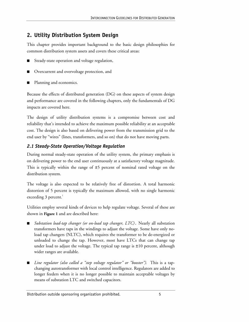
Utilities employ several kinds of devices to help regulate voltage. Several of these are
shown in Figure 1 and are described here:
■ Substation load-tap changer (or on-load tap changer, LTC). Nearly all substation transformers have taps in the windings to adjust the voltage. Some have only no-load tap changers (NLTC), which requires the transformer to be de-energized or unloaded to change the tap. However, most have LTCs that can change tap under load to adjust the voltage. The typical tap range is ±10 percent, although wider ranges are available.
■ Line regulator (also called a “step voltage regulator” or “booster”). This is a tap-changing autotransformer with local control intelligence. Regulators are added to longer feeders when it is no longer possible to maintain acceptable voltages by means of substation LTC and switched capacitors.
INTERCONNECTION GUIDELINES FOR DISTRIBUTED GENERATION
Distribution outside sponsoring organization prohibited. 6
■ Switched shunt capacitors. As the load grows on a feeder, the voltage profile along the feeder begins to sag. Capacitors are generally the first type of device a utility will add to the feeder to correct for this. They are usually the least expensive of the options for correcting for the effects of load current and have the added benefit of reducing the losses and freeing up line capacity. Though line regulators can boost the voltage, they do not significantly alter the loading.
Substation LTCs and line regulators behave similarly. They most commonly have 16
steps of raise (boost) taps and 16 steps of lower (buck) taps of 5/8 percent each.
Thus, they are frequently called “32-step” regulators. Modern controls are
microprocessor-based and have a wide variety of control options. In a typical
application, when the voltage goes out of band for a predetermined time delay
ranging from 15 to 45 seconds, the tap will change at a rate of about one tap every 2
seconds until the voltage is satisfactorily back within band. This is sufficiently fast for
the vast majority of load cycles experienced on a distribution feeder, although rapidly
changing loads may call for additional measures. Given the normal variation of load
on a feeder, a maximum of a dozen or so tap changes per day are expected. Excessive
numbers of tap changes can dramatically reduce the life of the LTC or regulator.
Figure 1: Voltage regulation system on a radial distribution feeder
In the U.S., LTCs are three-phase tap changers with one control for all three phases,
whereas line regulators are usually single-phase autotransformers with individual
controls for each phase. Regulators are normally installed in three-phase banks, but
they may also be installed in other connections, such as open-delta, which requires
only two regulators for a three-phase load. Regulators are also applied on longer
PRIMARYDISTRIBUTION
FEEDERS
SUBSTATIONLTC
TRANSMISSIONSYSTEM
FEEDER BREAKEROR RECLOSER
LINE REGULATOR
SWITCHED SHUNTCAPACITORS
INTERCONNECTION GUIDELINES FOR DISTRIBUTED GENERATION
Distribution outside sponsoring organization prohibited. 7
single-phase laterals. Some models allow all three phases to be ganged so that the
three phases operate together from one control.
Although it may seem that having three independently controlled autotransformers
would contribute to voltage unbalance, it often accomplishes better phase balance.
Distribution lines are typically constructed in an unbalanced configuration, and there
are many single-phase loads. This naturally leads to unbalance in the system. Single-
phase voltage regulators can actually compensate for some of the unbalance in the
voltage.
Some regulator controls can bypass the initial time delay if the voltage goes
sufficiently far out of band. Then the device proceeds directly into the 2-second tap
change sequence.
Typically, capacitor banks are sized in increments of 300 kilovolt amperes reactive
(kVAR) with typically no more than 2,400 kVAR in one location unless there is a
large load. An average size would be between 600 and 1,200 kVAR. Switching in a
capacitor bank would typically boost the voltage by 2 to 3 percent. Capacitors are
switched only once or twice per day. Controls usually rely on local measurements of
voltage, current, or volt amperes reactive (VAR). Many capacitors are simply
controlled by a time clock and switch at the same time each day.
It is important to have a basic understanding of how utility voltage regulation is
accomplished, because there are possible interactions between these devices and
distributed generation. Conflicts can arise when the generation either attempts to
regulate the voltage in opposition to the utility devices or the generation changes too
rapidly for the standard voltage regulation equipment to respond.
2.2 Overcurrent Protection
The structure of utility transmission and distribution systems is strongly influenced
by the needs of overcurrent protection. Faults (short circuits) are inevitable. Any
given system can be expected to suffer several faults each year. The number will
depend on exposure to lightning and trees as well as the age of the system’s
components. There is a wide range in this number. Some feeders will average less
than 1 interruption per year, while others might have more than 25.
When the short circuit occurs, the fault current must be interrupted quickly to
minimize damage so that electricity service can be promptly restored.
The number of breakers, or other fault interrupters, that must operate to clear the
fault depends on the design of the system. Transmission systems generally consist of
a highly meshed network of lines that interconnect numerous sources of power.
INTERCONNECTION GUIDELINES FOR DISTRIBUTED GENERATION
Distribution outside sponsoring organization prohibited. 8
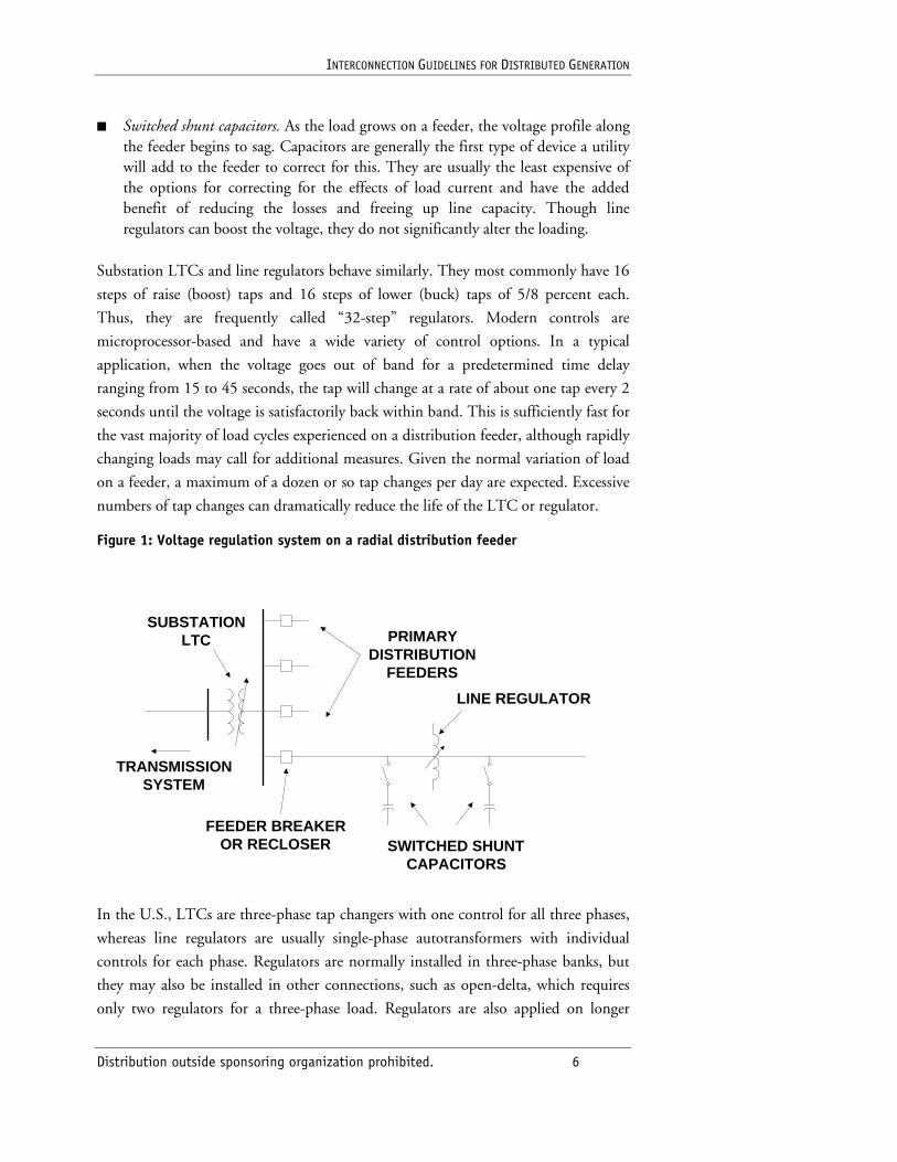
Transmission lines usually have fault interrupters at both ends. When a fault occurs
in a line, both interrupters must operate as shown in Figure 2, because the fault
current could be supplied from either end.
One advantage of transmission system protection is that it readily accepts new
generation. Also, generation directly connected to the transmission system tends to
be large, which makes interconnection cost less of an issue. An excellent protection
system represents only a minor portion of the entire generator system cost. In
contrast, this document concentrates on smaller generation connected to distribution
systems where interconnection cost is a significant portion of the total installation
cost.
In contrast with transmission systems, most distribution systems have been designed
with the assumption that the fault current contribution can come from only one
direction. There are two basic designs of distribution systems: radial systems and low-
voltage secondary networks. The design of each of these has been strongly influenced
by economics and simplicity of operation. There are many more distribution circuits
than transmission circuits, and the cost of protection is an extremely important factor
in distribution planning. Each feeder consists of numerous sections, and it is not
economically feasible to place fault interrupters at both ends of each section to better
accommodate distributed resources (DR). Therefore, DR installations must adapt to
the behavior of existing protection systems.
Figure 2: Clearing a fault on the transmission system
Radial System Protection
Radial systems usually cost the least to build. Their protection consists of a number
of overcurrent devices in series. Ideally, only one of these devices has to operate to
clear a fault—the nearest upline device. Customers on unaffected sections of the
Both Breakers
Must Operate
Fault
INTERCONNECTION GUIDELINES FOR DISTRIBUTED GENERATION
Distribution outside sponsoring organization prohibited. 9
feeder remain in service. Although this is the basic way the system operates, utilities
have added some relatively complex behaviors to some of the protective elements to
improve reliability.
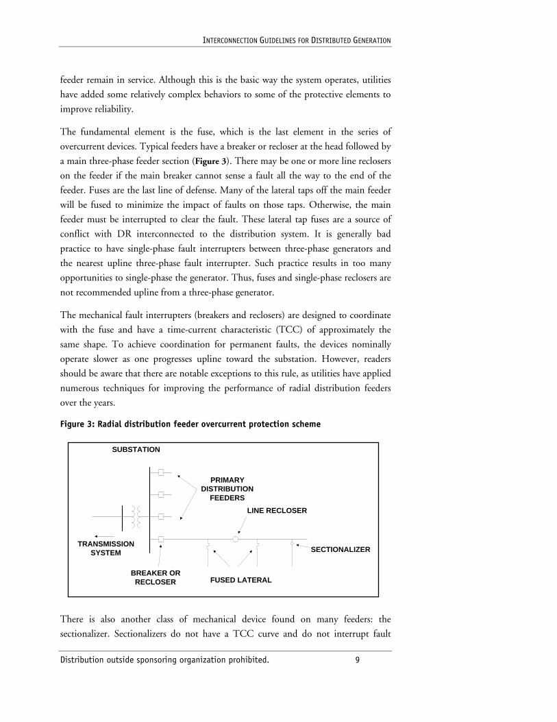
The fundamental element is the fuse, which is the last element in the series of
overcurrent devices. Typical feeders have a breaker or recloser at the head followed by
a main three-phase feeder section (Figure 3). There may be one or more line reclosers
on the feeder if the main breaker cannot sense a fault all the way to the end of the
feeder. Fuses are the last line of defense. Many of the lateral taps off the main feeder
will be fused to minimize the impact of faults on those taps. Otherwise, the main
feeder must be interrupted to clear the fault. These lateral tap fuses are a source of
conflict with DR interconnected to the distribution system. It is generally bad
practice to have single-phase fault interrupters between three-phase generators and
the nearest upline three-phase fault interrupter. Such practice results in too many
opportunities to single-phase the generator. Thus, fuses and single-phase reclosers are
not recommended upline from a three-phase generator.
The mechanical fault interrupters (breakers and reclosers) are designed to coordinate
with the fuse and have a time-current characteristic (TCC) of approximately the
same shape. To achieve coordination for permanent faults, the devices nominally
operate slower as one progresses upline toward the substation. However, readers
should be aware that there are notable exceptions to this rule, as utilities have applied
numerous techniques for improving the performance of radial distribution feeders
over the years.
Figure 3: Radial distribution feeder overcurrent protection scheme
There is also another class of mechanical device found on many feeders: the
sectionalizer. Sectionalizers do not have a TCC curve and do not interrupt fault
PRIMARYDISTRIBUTION
FEEDERS
SUBSTATION
TRANSMISSIONSYSTEM
BREAKER ORRECLOSER
LINE RECLOSER
SECTIONALIZER
FUSED LATERAL
INTERCONNECTION GUIDELINES FOR DISTRIBUTED GENERATION
Distribution outside sponsoring organization prohibited. 10
current. Instead, they have built-in intelligence to observe the behavior of the upline
recloser and isolate the faulted section after the interruption has occurred. They can
be either three-phase or single-phase. As with fuses, it is generally undesirable to have
single-phase sectionalizers upline from three-phase generators because of the single-
phasing issue.
The current must be interrupted to clear the fault. The radial system protection
expects fault current from only one direction and assumes the current can be
interrupted by operating one device. Therefore, any distributed resource on a radial
feeder must disconnect to permit the feeder protective devices to go through their
normal fault-clearing sequence.
Many faults on the system are temporary. Therefore, automatic reclosing of breakers
and reclosers is a nearly universal utility practice. Breakers and reclosers typically
make two to four attempts to clear the fault. Because most faults are temporary,
many breakers and reclosers are set to operate once or twice very quickly in an
attempt to save the lateral fuses so that a line crew does not have to be dispatched to
restore service.
Some of the conflicts with distributed resources that one might expect in the
protection scheme shown in Figure 3 include these:
■ DR infeed into the fault prevents the fault from clearing in the expected time.
■ DR infeed desensitizes the overcurrent devices so that they no longer detect all the faults as promptly as they would otherwise.
■ DR infeed may prevent the possibility of saving lateral fuses on temporary faults.
■ Fuses and single-phase reclosers and sectionalizers may have to be removed or replaced with three-phase switchgear.
■ Reclose intervals may have to be extended to ensure that the distributed resource has properly disconnected.
Each of these conflicts yields either higher interconnection costs or results in some
reduction in distribution system reliability.
Secondary Network Protection
The other major class of distribution design is depicted in Figure 4. Typically, there
are a number of feeders from the same substation supplying power to a low-voltage
secondary network in a downtown area or in an office complex. Single-facility
networks are commonly known as “spot networks.” The purpose of this design is to
INTERCONNECTION GUIDELINES FOR DISTRIBUTED GENERATION
Distribution outside sponsoring organization prohibited. 11
achieve very high reliability, and it is more expensive to build than the simple radial
system. The system is designed to take at least one fault on any of the primary feeders
without interrupting power to any of the customers served from the low-voltage
network. Interruptions are expected only when there is a major transmission failure.
Some network systems are designed to sustain two failures on the primary
distribution feeders.
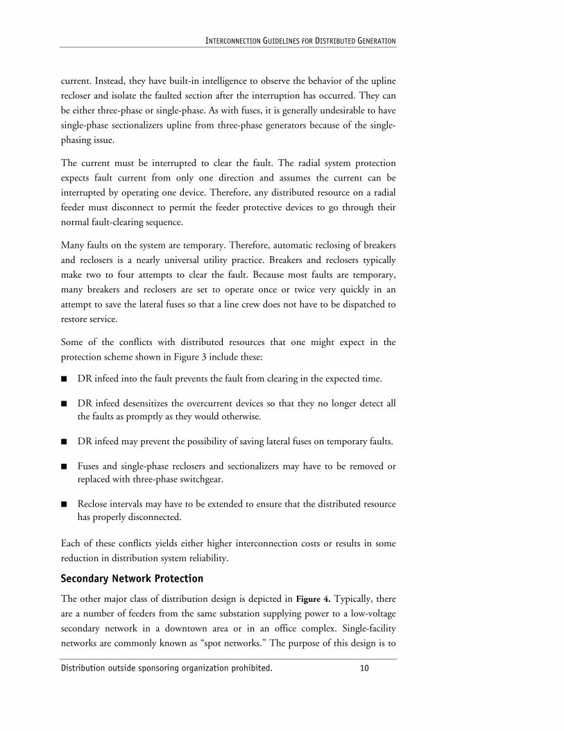
Figure 4: Protection for a low-voltage secondary network system
SUBSTATION
TRANSMISSIONSYSTEM
FEEDER BREAKEROR RECLOSER
THESE DEVICESMUST OPERATE
FAULT
LOW-VOLTAGE NETWORK
NETWORKPROTECTOR
PRIMARY FEEDERS
In the design depicted in Figure 4, there are four primary voltage feeders serving the
network. Network transformers are spaced periodically along these feeders,
transferring power from the primary feeders to the low-voltage network. Each
network transformer is paired with a special fault interrupter called a “network
protector.” The network is an extensively meshed system of wires interconnecting the
loads. Ideally, each load point would have at least two network lines feeding it so that
service would continue if one failed.
In the U.S. there are two popular voltages for secondary networks: 480 volt (V) and
120/208 V.
The secondary network interconnects all the feeders. Therefore, when a fault occurs
on one feeder, current will be fed back through the network from the other feeders,
as shown in Figure 4. Not only must the feeder breaker operate, but all the network
protectors connected to the faulted feeder must open to interrupt all contributions to
the fault.
INTERCONNECTION GUIDELINES FOR DISTRIBUTED GENERATION
Distribution outside sponsoring organization prohibited. 12
To accomplish this automatically, network protectors are relayed to trip on reverse
power on the presumption that the only time power would flow opposite the normal
direction is when there is a fault on the primary distribution feeder. To prevent
energizing the network transformer from the secondary, these relays may be set to be
very sensitive, and it takes very little reverse power to trip the network protector. This
is the source of the chief difficulty in applying distributed resources on secondary
networks and limits the maximum DR capacity to a fraction of the minimum load. If
there is a net export of power from the network, even for an instant, all of the
network protectors can be tripped, which defeats the main purpose for having such a
network.
Some networks must be arranged so that the load is distributed among the primary
feeders to achieve a satisfactory voltage balance between the feeders. Otherwise, some
network protectors would trip during normal operation or minor system
disturbances. The introduction of distributed resources into the network could
change the load profile within the network such that the voltage balance between the
feeders is adversely affected. This would increase the number of inadvertent network
protector operations.
2.3 Planning and Economics
Much of the economic benefit of distributed resources is realized when the DR is
installed for end-use applications. Factories with high-value products will find
backup power attractive, and it may be possible to economically interconnect that
generation for the mutual benefit of the utility and the end user. Backup generation
might be operated at peak demand times to help utilities cover contingencies until
such time as the utility makes an investment in additional wire capacity. If the
arrangement has sufficient economic merit and the generation proves reliable, the
utility may defer transmission and distribution (T&D) expenditures indefinitely.
Another area in which there are quite favorable economics on the end-use side is
combined heat and power (CHP). Many commercial and industrial sites have
thermal loads as well as electrical loads and are consuming natural gas or some other
fuel to supply their thermal needs. These facilities can benefit economically from
CHP applications that use waste heat from the electricity generation process to satisfy
the thermal demand, with resultant high net efficiency. CHP applications are often
interconnected with the utility system at least part of the day.
Where is the potential benefit of DR to utilities? How can planning engineers
determine if and when DR might be an economical solution to a planning problem?
This issue is one on which an entire book can be written. Here we will make some
basic suggestions for how to go about making the evaluation. Figure 5 shows a

INTERCONNECTION GUIDELINES FOR DISTRIBUTED GENERATION
Distribution outside sponsoring organization prohibited. 13
multilevel screening process for evaluating a DR application for utility distribution
planning.2
Figure 5: Four-step progressive screen for planning with distributed resources
The first level is strictly performed using economics. The marginal cost of
implementing T&D upgrade (“wires”) solutions is compared against the marginal
cost of DR technologies. This screens out many possibilities quickly. Besides
investment costs, value-of-service indicators can be used as well as measures of costs
associated with wholesale power price volatility. As we move down the process, the
analysis gets increasingly specific. The second level is a more detailed economic
screen that includes some simulations of the electrical system in moderate detail. This
takes a closer look at how proposed DR solutions might yield economic benefit.
From the utility perspective, often only the lowest-cost technologies—diesel gensets
or combustion turbines—are attractive after passing through these two screens.
Higher-cost technologies may still be attractive to an end user, and the utility may
choose to partially subsidize particular applications that provide benefit. However,
the utility must be careful not to pay more than the marginal costs identified in these
two screens for lower-cost alternatives. The third level takes a look at the DR
candidates that survive the previous screens and ranks them from the engineering
perspective. At the bottom level, a candidate DR solution has been selected and
requirements for interconnection and operation are determined. This is the only step
in the process familiar to many utility distribution engineers. However, several
interesting things occur before deciding to install DR.
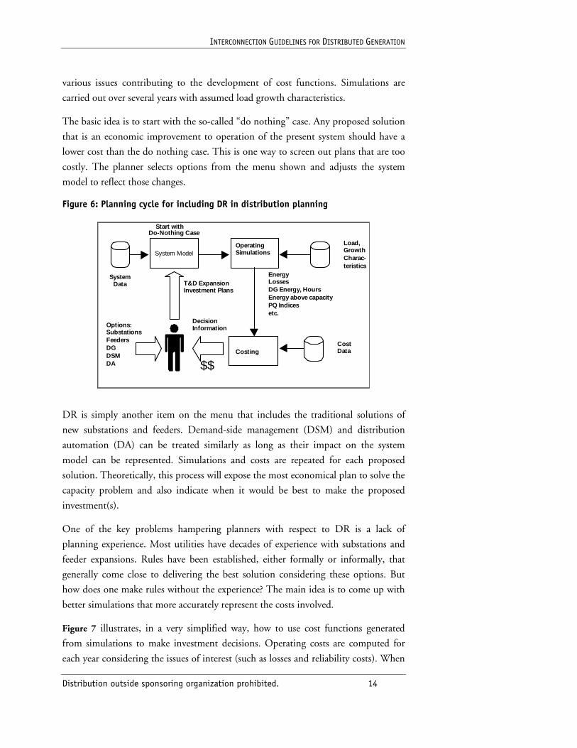
One process that can include DR and that is effective for the middle two screening
levels is depicted in Figure 6. The cycle begins with a system model that is built from
the data describing the impedances, loads, and so on. The system is simulated with
T&D Marginal Cost Screen
High-Level Feasibility Screen
Engineering Screen
Implementation Studies
T&D Marginal Cost Screen
High-Level Feasibility Screen
Engineering Screen
Implementation Studies
INTERCONNECTION GUIDELINES FOR DISTRIBUTED GENERATION
Distribution outside sponsoring organization prohibited. 14
various issues contributing to the development of cost functions. Simulations are
carried out over several years with assumed load growth characteristics.
The basic idea is to start with the so-called “do nothing” case. Any proposed solution
that is an economic improvement to operation of the present system should have a
lower cost than the do nothing case. This is one way to screen out plans that are too
costly. The planner selects options from the menu shown and adjusts the system
model to reflect those changes.
Figure 6: Planning cycle for including DR in distribution planning
System ModelOperatingSimulations
Costing
SystemData T&D Expansion
Investment Plans
DecisionInformation
Start with Do-Nothing Case
EnergyLossesDG Energy, HoursEnergy above capacityPQ Indicesetc.
$$
Options:SubstationsFeedersDGDSMDA
Load,GrowthCharac-teristics
CostData
DR is simply another item on the menu that includes the traditional solutions of
new substations and feeders. Demand-side management (DSM) and distribution
automation (DA) can be treated similarly as long as their impact on the system
model can be represented. Simulations and costs are repeated for each proposed
solution. Theoretically, this process will expose the most economical plan to solve the
capacity problem and also indicate when it would be best to make the proposed
investment(s).
One of the key problems hampering planners with respect to DR is a lack of
planning experience. Most utilities have decades of experience with substations and
feeder expansions. Rules have been established, either formally or informally, that
generally come close to delivering the best solution considering these options. But
how does one make rules without the experience? The main idea is to come up with
better simulations that more accurately represent the costs involved.
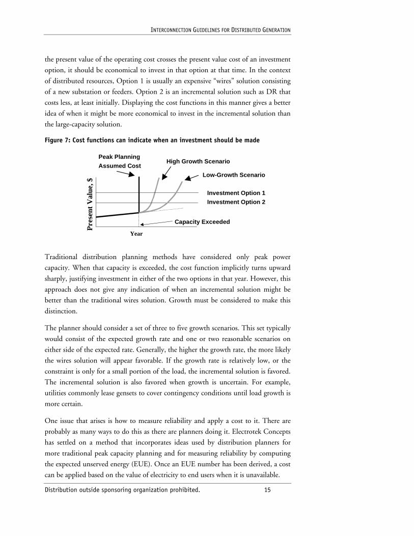
Figure 7 illustrates, in a very simplified way, how to use cost functions generated
from simulations to make investment decisions. Operating costs are computed for
each year considering the issues of interest (such as losses and reliability costs). When
INTERCONNECTION GUIDELINES FOR DISTRIBUTED GENERATION
Distribution outside sponsoring organization prohibited. 15
the present value of the operating cost crosses the present value cost of an investment
option, it should be economical to invest in that option at that time. In the context
of distributed resources, Option 1 is usually an expensive “wires” solution consisting
of a new substation or feeders. Option 2 is an incremental solution such as DR that
costs less, at least initially. Displaying the cost functions in this manner gives a better
idea of when it might be more economical to invest in the incremental solution than
the large-capacity solution.
Figure 7: Cost functions can indicate when an investment should be made
Year
Pre
sent
Val
ue, $
High Growth Scenario
Low-Growth Scenario
Investment Option 1
Investment Option 2
Capacity Exceeded
Peak Planning
Assumed Cost
Traditional distribution planning methods have considered only peak power
capacity. When that capacity is exceeded, the cost function implicitly turns upward
sharply, justifying investment in either of the two options in that year. However, this
approach does not give any indication of when an incremental solution might be
better than the traditional wires solution. Growth must be considered to make this
distinction.
The planner should consider a set of three to five growth scenarios. This set typically
would consist of the expected growth rate and one or two reasonable scenarios on
either side of the expected rate. Generally, the higher the growth rate, the more likely
the wires solution will appear favorable. If the growth rate is relatively low, or the
constraint is only for a small portion of the load, the incremental solution is favored.
The incremental solution is also favored when growth is uncertain. For example,
utilities commonly lease gensets to cover contingency conditions until load growth is
more certain.
One issue that arises is how to measure reliability and apply a cost to it. There are
probably as many ways to do this as there are planners doing it. Electrotek Concepts
has settled on a method that incorporates ideas used by distribution planners for
more traditional peak capacity planning and for measuring reliability by computing
the expected unserved energy (EUE). Once an EUE number has been derived, a cost
can be applied based on the value of electricity to end users when it is unavailable.
INTERCONNECTION GUIDELINES FOR DISTRIBUTED GENERATION
Distribution outside sponsoring organization prohibited. 16
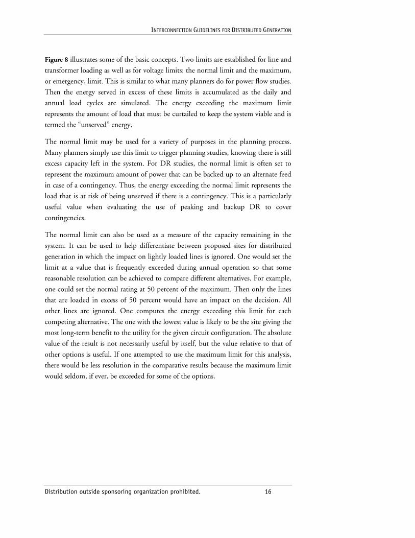
Figure 8 illustrates some of the basic concepts. Two limits are established for line and
transformer loading as well as for voltage limits: the normal limit and the maximum,
or emergency, limit. This is similar to what many planners do for power flow studies.
Then the energy served in excess of these limits is accumulated as the daily and
annual load cycles are simulated. The energy exceeding the maximum limit
represents the amount of load that must be curtailed to keep the system viable and is
termed the “unserved” energy.
The normal limit may be used for a variety of purposes in the planning process.
Many planners simply use this limit to trigger planning studies, knowing there is still
excess capacity left in the system. For DR studies, the normal limit is often set to
represent the maximum amount of power that can be backed up to an alternate feed
in case of a contingency. Thus, the energy exceeding the normal limit represents the
load that is at risk of being unserved if there is a contingency. This is a particularly
useful value when evaluating the use of peaking and backup DR to cover
contingencies.
The normal limit can also be used as a measure of the capacity remaining in the
system. It can be used to help differentiate between proposed sites for distributed
generation in which the impact on lightly loaded lines is ignored. One would set the
limit at a value that is frequently exceeded during annual operation so that some
reasonable resolution can be achieved to compare different alternatives. For example,
one could set the normal rating at 50 percent of the maximum. Then only the lines
that are loaded in excess of 50 percent would have an impact on the decision. All
other lines are ignored. One computes the energy exceeding this limit for each
competing alternative. The one with the lowest value is likely to be the site giving the
most long-term benefit to the utility for the given circuit configuration. The absolute
value of the result is not necessarily useful by itself, but the value relative to that of
other options is useful. If one attempted to use the maximum limit for this analysis,
there would be less resolution in the comparative results because the maximum limit
would seldom, if ever, be exceeded for some of the options.
INTERCONNECTION GUIDELINES FOR DISTRIBUTED GENERATION
Distribution outside sponsoring organization prohibited. 17
Figure 8: Basic concept for establishing limits for computing costs related to system capacity limits
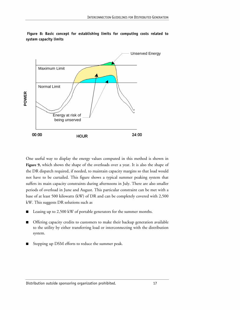
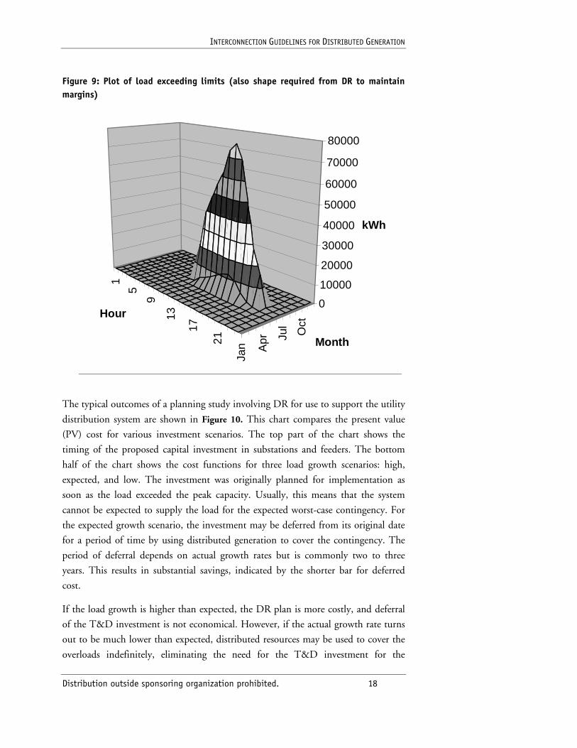
One useful way to display the energy values computed in this method is shown in
Figure 9, which shows the shape of the overloads over a year. It is also the shape of
the DR dispatch required, if needed, to maintain capacity margins so that load would
not have to be curtailed. This figure shows a typical summer peaking system that
suffers its main capacity constraints during afternoons in July. There are also smaller
periods of overload in June and August. This particular constraint can be met with a
base of at least 500 kilowatts (kW) of DR and can be completely covered with 2,500
kW. This suggests DR solutions such as
■ Leasing up to 2,500 kW of portable generators for the summer months.
■ Offering capacity credits to customers to make their backup generation available to the utility by either transferring load or interconnecting with the distribution system.
■ Stepping up DSM efforts to reduce the summer peak.
PO
WE
R
Maximum Limit
Normal Limit
Energy at risk ofbeing unserved
Unserved Energy
INTERCONNECTION GUIDELINES FOR DISTRIBUTED GENERATION
Distribution outside sponsoring organization prohibited. 18
Figure 9: Plot of load exceeding limits (also shape required from DR to maintain margins)
1
5
9
13
17
21
Jan Apr Ju
l
Oct
0
10000
20000
30000
40000
50000
60000
70000
80000
kWh
Hour
Month
The typical outcomes of a planning study involving DR for use to support the utility
distribution system are shown in Figure 10. This chart compares the present value
(PV) cost for various investment scenarios. The top part of the chart shows the
timing of the proposed capital investment in substations and feeders. The bottom
half of the chart shows the cost functions for three load growth scenarios: high,
expected, and low. The investment was originally planned for implementation as
soon as the load exceeded the peak capacity. Usually, this means that the system
cannot be expected to supply the load for the expected worst-case contingency. For
the expected growth scenario, the investment may be deferred from its original date
for a period of time by using distributed generation to cover the contingency. The
period of deferral depends on actual growth rates but is commonly two to three
years. This results in substantial savings, indicated by the shorter bar for deferred
cost.
If the load growth is higher than expected, the DR plan is more costly, and deferral
of the T&D investment is not economical. However, if the actual growth rate turns
out to be much lower than expected, distributed resources may be used to cover the
overloads indefinitely, eliminating the need for the T&D investment for the
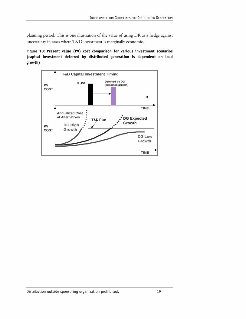
INTERCONNECTION GUIDELINES FOR DISTRIBUTED GENERATION
Distribution outside sponsoring organization prohibited. 19
planning period. This is one illustration of the value of using DR as a hedge against
uncertainty in cases where T&D investment is marginally economic.
Figure 10: Present value (PV) cost comparison for various investment scenarios (capital investment deferred by distributed generation is dependent on load growth)
PVCOST
TIME
T&D Capital Investment Timing
PVCOST
TIME
DG HighGrowth
DG ExpectedGrowth
DG LowGrowth
Annualized Costof Alternatives
T&D Plan
No DGDeferred by DG(expected growth)
INTERCONNECTION GUIDELINES FOR DISTRIBUTED GENERATION
Distribution outside sponsoring organization prohibited. 20
3. DR Interconnection Technologies
The range and diversity of distributed generation (DG) technologies is large relative
to the much more familiar technology of central station electric generation plants. A
variety of fuels and prime movers are used—from the radiant energy of the sun with
photovoltaic modules, to chemical reactions in fuel cells, to conventional diesel or
natural gas–engines and gas turbines. For purposes of this guide, however, the energy
conversion process is not of primary importance to evaluations of how DG
installations affect the performance of distribution systems to which they are
connected.
Despite the wide range of technologies and energy-conversion processes found in DG
technology, as pertains to the interface with the external electric power system,
distributed resources (DR) come in two major types: rotating electric machines and
static electrical power inverters. For purposes of electric power system analyses, it is
the behavior of this last stage of the conversion process—from whatever form to AC
electric energy compatible in voltage, frequency, and phase angle with the external
electric power system—that is of primary importance.
Engineering evaluations of the “impacts” of an element that is to be connected to the
power system employ a range of analytical techniques; these techniques form the
basis for computer simulation or calculation routines that have become standard
practice for power system designers. The studies in which these tools are used allow
the engineer to “see the system” as it will behave or operate before the element is
actually installed. This is especially true for evaluations of DG interconnections,
because they would normally be conducted prior to actual installation or
commissioning of the unit in question.
As such, the ability to represent, or model, the distributed generator is a critical part
of the engineering evaluation process that has been successfully used for more than a
century to manage one of the most complex machines ever created—the
interconnected electric power system. In contrast with more conventional electric
generation equipment, DG technologies are generally not as well known or
understood, and many times they incorporate equipment or controls that are
unfamiliar to the utility engineering community. This section provides an overview
of the common interfaces for DG systems and discusses approaches for considering
such devices and equipment in analytical procedures.
3.1 DG Models for Power System Studies
The appropriate representation of an electric power system element is greatly
dependent on the purpose and objective of the analytical procedure. Representations
INTERCONNECTION GUIDELINES FOR DISTRIBUTED GENERATION
Distribution outside sponsoring organization prohibited. 21
of the same element will vary depending on the type of analysis to be performed. In
evaluating the possible impacts of DG installations on distribution system
performance, the most common analyses consist of two general types of idealized
system models typically used in distribution system evaluation: power flow
calculations and short-circuit calculations.
Results of these basic analyses are used to evaluate a number of fundamental
distribution system performance aspects, including voltage regulation, thermal
capabilities/loading, protection system behavior, and delivery losses. Less frequently,
other studies may be necessary to evaluate technical issues such as harmonics, voltage
flicker, or dynamic response to disturbances on the power system.
3.2 Characteristics of DG Interface Technologies: Rotating Machines
Synchronous Generators
Synchronous generators are by far the most common device for converting kinetic
energy in a rotating shaft to electric energy. Electrically, synchronous machines
consist of a three-phase stationary winding (stator) connected to the three phases of
the power supply system and a winding on the rotor to which a source of DC
excitation is applied.
Volumes of technical papers and textbooks have been written on the principles of
synchronous generator control. There are two primary control mechanisms: the
speed governor on the prime mover driving the machine and the excitation control
system, which supplies DC potential to field winding and regulates field current.
Power control in a synchronous generator is the responsibility of the governor on the
prime mover. By changing the mechanical torque applied to the rotating system (for
example, by increasing steam flow to turbine blades), the speed of the system will
either increase or decrease, depending on the algebraic sign of the change. As it does,
the rotor of the synchronous generator either moves forward or backward relative to
the synchronously rotating stator field in the machine, which is fixed by the
frequency of the power system. The angle of synchronous generator rotor with
respect to the synchronously rotating stator field is called the “torque angle,” and for
a constant terminal voltage directly determines the real power flowing into or out of
the terminals. Because the generator must run in precise synchronicity with the
electric grid, changes in grid frequency will result in changes in real power output of
the distributed generator.
Reactive power output of a synchronous generator can be controlled by adjusting the
DC voltage applied to the field winding to affect a change in the field current.
INTERCONNECTION GUIDELINES FOR DISTRIBUTED GENERATION
Distribution outside sponsoring organization prohibited. 22
To ensure system security and reliability in interconnected bulk power networks,
control mechanisms of individual large generators must be coordinated. Frequency-
sensitive governors with coordinated droop settings are used to assist with system
frequency regulation and to apportion incremental changes in load among various
generating units. Excitation control systems are tuned to ensure proper steady-state
voltage regulation and provide dynamic voltage support during disturbances for
system recovery. In smaller installations, as would be the case for distributed
generators, a wider variation in the control mechanisms and parameters is found,
because their individual impact on the grid would be small. Governors may be set to
regulate real power generation independent of system frequency variations, and
excitation controllers may utilize a constant power factor or reactive power reference
instead of bus voltage signal to control reactive power.
Modeling synchronous generators and the various auxiliary control equipment for
power system studies is a fairly well-developed art. In utility short-circuit
calculations, simplified generator models consisting of an internal voltage source in
series with an equivalent reactance are usually employed (Figure 11).
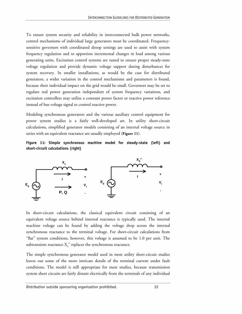
Figure 11: Simple synchronous machine model for steady-state (left) and short-circuit calculations (right)
In short-circuit calculations, the classical equivalent circuit consisting of an
equivalent voltage source behind internal reactance is typically used. The internal
machine voltage can be found by adding the voltage drop across the internal
synchronous reactance to the terminal voltage. For short-circuit calculations from
“flat” system conditions, however, this voltage is assumed to be 1.0 per unit. The
subtransient reactance Xd" replaces the synchronous reactance.
The simple synchronous generator model used in most utility short-circuit studies
leaves out some of the more intricate details of the terminal current under fault
conditions. The model is still appropriate for most studies, because transmission
system short circuits are fairly distant electrically from the terminals of any individual
Eg
Xd’’
I
Vt
+
-
Eg
Xs
I
Vt
+
-P, Q
INTERCONNECTION GUIDELINES FOR DISTRIBUTED GENERATION
Distribution outside sponsoring organization prohibited. 23
generator. This may not be the case on distribution systems with distributed
generators, however.
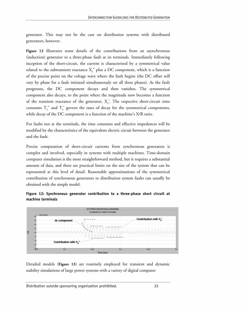
Figure 12 illustrates some details of the contributions from an asynchronous
(induction) generator to a three-phase fault at its terminals. Immediately following
inception of the short-circuit, the current is characterized by a symmetrical value
related to the subtransient reactance Xd" plus a DC component, which is a function
of the precise point on the voltage wave where the fault begins (the DC offset will
vary by phase for a fault initiated simultaneously on all three phases). As the fault
progresses, the DC component decays and then vanishes. The symmetrical
component also decays, to the point where the magnitude now becomes a function
of the transient reactance of the generator, Xd’. The respective short-circuit time
constants Td" and Td’ govern the rates of decay for the symmetrical components,
while decay of the DC component is a function of the machine’s X/R ratio.
For faults not at the terminals, the time constants and effective impedances will be
modified by the characteristics of the equivalent electric circuit between the generator
and the fault.
Precise computation of short-circuit currents from synchronous generators is
complex and involved, especially in systems with multiple machines. Time-domain
computer simulation is the most straightforward method, but it requires a substantial
amount of data, and there are practical limits on the size of the system that can be
represented at this level of detail. Reasonable approximations of the symmetrical
contribution of synchronous generators to distribution system faults can usually be
obtained with the simple model.
Figure 12: Synchronous generator contribution to a three-phase short circuit at machine terminals
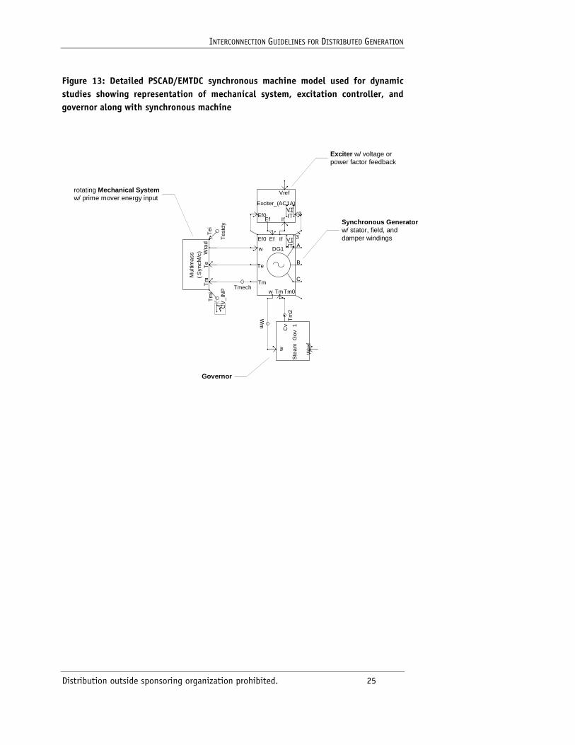
Detailed models (Figure 13) are routinely employed for transient and dynamic
stability simulations of large power systems with a variety of digital computer
12.5 MVA Synchronous Generator
Time (sec)
Contribution to Fault at Terminals
5.75 5.9 6.05 6.2 6.35 6.5
kA
-8
-6
-4
-2
+0
+2
+4
+6
+8SG Current
Contribution with Xd’
Contribution with Xd’’
dc component
INTERCONNECTION GUIDELINES FOR DISTRIBUTED GENERATION
Distribution outside sponsoring organization prohibited. 24
programs. In these models, the generator, governor, excitation control, and
sometimes the prime mover (such as steam or gas turbine, boiler, or hydraulic
system) are represented by differential equations that are solved at successive
increments of time, along with the power flow equations for electric network to
which they are connected. It is not yet clear to what extent stability studies and
dynamic simulations will become necessary for distribution systems with distributed
generation.
Synchronous generators are normally considered to be linear devices, that is, the
voltages and currents generated are perfectly sinusoidal. This assumption is less
accurate for smaller machines for reasons associated with the distribution of the
individual windings in the slots of the machine stator. Under certain situations,
harmonics can be an issue with small rotating machines, although the degree of
distortion is much less than that associated with familiar nonlinear loads. Section 5
contains a description of some harmonic issues related to small rotating machinery.
Typical parameters for synchronous machines used in models like that shown in
Figure 13 are found in Table 1.
INTERCONNECTION GUIDELINES FOR DISTRIBUTED GENERATION
Distribution outside sponsoring organization prohibited. 25
Figure 13: Detailed PSCAD/EMTDC synchronous machine model used for dynamic studies showing representation of mechanical system, excitation controller, and governor along with synchronous machine
Te
std
yC
V_I
NP
Wm
Tmech
VTIT 3
IfEfEf0
Vref
Exciter_(AC1A)
Tm
2
( Syn
cM/c
)M
ultim
ass
Te
Wra
dT
mT
mi
Tei
w
Wre
f
Cv
Ste
am G
ov
1
DG1
Ef0 Ef If VTIT
3
Tm0Tmw
w
Te
Tm
A
B
C
Exciter w/ voltage orpower factor feedback
Governor
rotating Mechanical Systemw/ prime mover energy input
Synchronous Generatorw/ stator, field, anddamper windings

INTERCONNECTION GUIDELINES FOR DISTRIBUTED GENERATION
Distribution outside sponsoring organization prohibited. 26
Table 1: Typical equivalent circuit parameters for small synchronous generators (impedances in per unit)
.BDIJOF
7BMVF " # $ %
kVA 69 156 781 1044
kW 55 125 625 835
V 480 480 480 480
pf .80 .80 .80 .80
n(r/min) 1,800 1,800 1,800 1,800
H .329 .205 .500 .535
Xd 2.02 6.16 2.43 2.38
Xd’ .171 .347 .254 .264
Xd" .087 .291 .207 .201
Xq 1.06 2.49 1.12 1.10
Xq" .163 .503 .351 .376
τdo’ (s) .950 1.87 1.90 2.47
τdo" (s) .078 .013 .024 .018
τqo" (s) .045 .020 .016 .009
ra .011 .034 .017 .013
τa (s) .014 .022 .038 .032
X0 .038 .054 .051 .074
X2 .125 .375 .279 .260
IFD base (A) 9.5 5.6 16.75 16.2
SG (1.0) .46 .207 .164 .099
SG (1.2) 1.45 1.00 .625 .569
Induction Generators
Induction generators are essentially induction motors that are driven at speeds above
their nameplate synchronous speed by some prime mover. The machine consists of a
INTERCONNECTION GUIDELINES FOR DISTRIBUTED GENERATION
Distribution outside sponsoring organization prohibited. 27
three-phase stationary winding connected to the three phases of the power supply—
much like that found in a synchronous machine—and a second assemblage of real or
virtual windings on the rotor. Wound-rotor induction machines have a three-phase
winding on the rotor structure that’s accessible externally via slip-ring connections.
In squirrel cage induction machines, by far the most common type, the rotor
windings are actually constituted by “bars” connected between two conductive rings,
one at each end of the rotor. The bars are physically embedded into the rotor
structure, resulting in a degree of robustness and reliability not found in other
electrical machines.
Because an induction machine has no field winding, the excitation necessary for
torque production and power flow must be drawn from the power supply system.
The electric current necessary for magnetizing the iron core is responsible for much
of the reactive power required by an induction machine.
Currents flowing in the rotor circuits are the other part of the torque-production
equation. Setting up these currents requires that a voltage be induced into the rotor
circuit. Relative motion—that is, a speed difference—between the rotor circuits and
the revolving magnetic field established by the stator windings, is the source of this
induced voltage. At synchronous speed, the relative motion between the rotor circuits
and the stator field is zero, and no voltage is induced in the rotor circuits. However,
if the rotor circuits move faster or slower than the synchronously rotating stator field,
voltages are induced that have a magnitude and frequency proportional to this speed
difference. Slip in an induction machine is a measure of this relative speed difference.
Under normal operating conditions, the slip varies in a nearly linear fashion with
load or generation. For example, in a machine rated for 2 percent slip at full load (or
generation), the slip value at 50 percent load (or generation) will be approximately 1
percent.
The variation of induction machine speed with torque provides for a much “softer”
coupling between the electric power system and the mechanical system driving the
machine. Induction generators also exhibit an inherent damping behavior for power
system disturbances. For example, if power system frequency increases—an
indication of generation in excess of load—this higher frequency actually reduces the
magnitude of slip in the induction generator, leading to a temporary reduction of
output—the exact remedy for high system frequency.
Reactive power is required by all induction machines and is normally drawn from the
supply system connected to the stator terminals. Even under no-load or no-
generation conditions, a substantial amount of reactive power is required by the
INTERCONNECTION GUIDELINES FOR DISTRIBUTED GENERATION
Distribution outside sponsoring organization prohibited. 28
machine. Reactive power will then increase as the stator current increases (in either
generator or motor mode).
Shunt capacitor banks are typically used to improve the power factor of induction
motors and generators. Standard practice is to compensate for most or all of the no-
load reactive power with fixed capacitor banks (generally switched with large
induction machines and switched banks), which are staged on or off, depending on
the desired compensated power factor as the load or generation conditions in the
machine change.
When the source of excitation—the power supply system, in most cases—is removed
from an induction machine, the main flux field collapses and torque production or
power flow is no longer possible. It does take several cycles for this field to collapse,
however, during which time an induction machine will contribute current to a short
circuit on the power system. Also, if voltage is just reduced rather than removed
completely as the result of a downstream fault, the main flux will decay to some new
value but will provide necessary excitation for the machine to contribute to the fault.
Contributions from end-use induction motors are rarely considered in utility fault
studies, although they can be an important consideration for protective device
coordination and rating within some industrial facilities. The IEEE Brown Book
(Standard 399-1997) “IEEE Recommended Practice for Industrial and Commercial
Power Systems Analysis” details procedures for calculating induction motor and
generator contributions to short circuits within facilities. A similar approach can be
employed for DG installations employing induction generators, but the differences
between industrial protection equipment and those utilized for medium-voltage
utility feeders in terms of operating and clearing times and device coordination must
be taken into consideration.
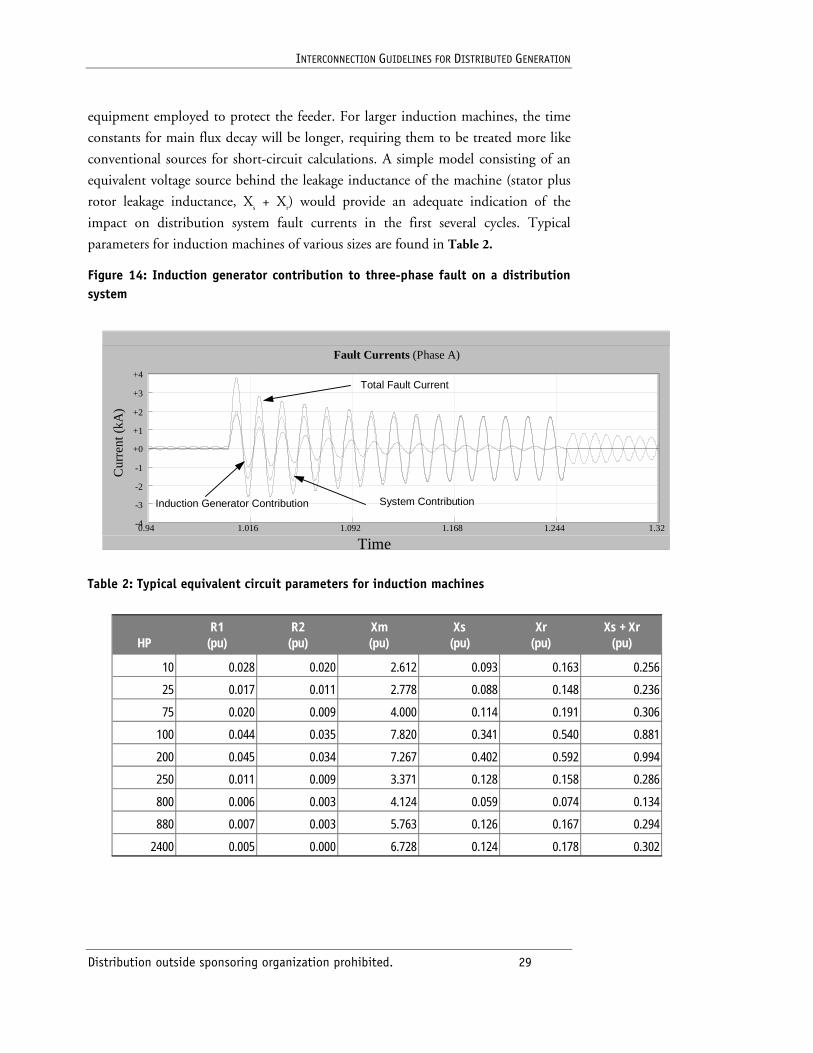
The effect of a DG installation on distribution system fault currents is illustrated in
Figure 14. Here it is assumed that the fault location is downline from the point on
the radial feeder to which the distributed generator installation is connected. This
relatively large DG plant consists of ten 750-kW wind turbines that use line-
connected squirrel-cage induction generators. Initially, the short-circuit current
contributed by the induction generators is nearly a great as that from the feeder
source. It contains both a symmetrical and DC component. As the fault progresses,
the induction generator contribution decreases as the main flux in the machine
decays. By the time the fault is cleared, the contribution from the induction
generators has nearly vanished.
How induction generators in DG applications should be treated for short-circuit
calculations will depend on the relative size of the DG plants and the type of
INTERCONNECTION GUIDELINES FOR DISTRIBUTED GENERATION
Distribution outside sponsoring organization prohibited. 29
equipment employed to protect the feeder. For larger induction machines, the time
constants for main flux decay will be longer, requiring them to be treated more like
conventional sources for short-circuit calculations. A simple model consisting of an
equivalent voltage source behind the leakage inductance of the machine (stator plus
rotor leakage inductance, Xs + Xr) would provide an adequate indication of the
impact on distribution system fault currents in the first several cycles. Typical
parameters for induction machines of various sizes are found in Table 2.
Figure 14: Induction generator contribution to three-phase fault on a distribution system
Table 2: Typical equivalent circuit parameters for induction machines
Time
Fault Currents (Phase A)
0.94 1.016 1.092 1.168 1.244 1.32 -4 -3 -2 -1 +0 +1 +2 +3 +4
Total Fault Current
System Contribution Induction Generator Contribution
Cur
rent
(kA
)
HPR1
(pu)R2
(pu)Xm (pu)
Xs (pu)
Xr (pu)
Xs + Xr (pu)
10 0.028 0.020 2.612 0.093 0.163 0.256
25 0.017 0.011 2.778 0.088 0.148 0.236
75 0.020 0.009 4.000 0.114 0.191 0.306
100 0.044 0.035 7.820 0.341 0.540 0.881
200 0.045 0.034 7.267 0.402 0.592 0.994
250 0.011 0.009 3.371 0.128 0.158 0.286
800 0.006 0.003 4.124 0.059 0.074 0.134
880 0.007 0.003 5.763 0.126 0.167 0.294
2400 0.005 0.000 6.728 0.124 0.178 0.302
INTERCONNECTION GUIDELINES FOR DISTRIBUTED GENERATION
Distribution outside sponsoring organization prohibited. 30
3.3 Characteristics of DG Interface Technologies: Static Power Converters
Certain DG technologies produce electrical energy in a form not compatible with a
fixed-voltage, fixed-frequency AC power system. Static power converters are
increasingly employed to effect the required electrical conversion, either from DC or
variable voltage, variable-frequency alternating current. Somewhat of a novelty or
confined to a few niche applications only 25 years ago, power electronics technology
has advanced tremendously, with new semiconductor switching devices, control
techniques, and converter technologies now impacting nearly all aspects of electric
energy utilization.
From the power system perspective, there are two basic types of static power
converters: line-commutated and self-commutated. Only a decade ago, there might
have been some question regarding which basic type might be employed in a DG
application. However, today, the more advanced and capable self-commutated
equipment is used almost exclusively. For this reason, the focus of this section is on
these more advanced converters.
A modern static power converter utilizes power semiconductor devices (that is,
switches) that are capable of both controlled turn-on as well as turn-off. Further, the
device characteristics enable switch transitions to occur very rapidly relative to a
single cycle of 60-hertz (Hz) voltage—nominal switching frequencies of a couple to
several kilohertz (kHz) are typical. This rapid switching speed, in combination with
very powerful and inexpensive digital control, provides several advantages for DG
interface applications:
■ Low waveform distortion with little expensive passive filtering.
■ High-performance regulating capability.
■ High conversion efficiency.
■ Fast response to abnormal conditions, including disturbances such as short circuits on the power system.
■ Capability for reactive power control.
Some DG technologies, such as fuel cells and photovoltaic modules, use energy-
conversion processes that result in electric power in the form of direct current.
Microturbines and some types of variable-speed wind generation produce electric
power where both the voltage magnitude and frequency vary. Static power
INTERCONNECTION GUIDELINES FOR DISTRIBUTED GENERATION
Distribution outside sponsoring organization prohibited. 31
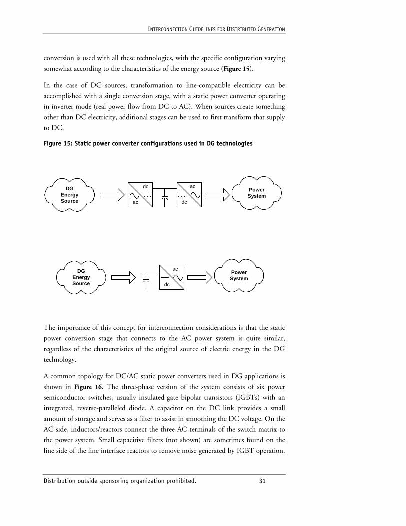
conversion is used with all these technologies, with the specific configuration varying
somewhat according to the characteristics of the energy source (Figure 15).
In the case of DC sources, transformation to line-compatible electricity can be
accomplished with a single conversion stage, with a static power converter operating
in inverter mode (real power flow from DC to AC). When sources create something
other than DC electricity, additional stages can be used to first transform that supply
to DC.
Figure 15: Static power converter configurations used in DG technologies
The importance of this concept for interconnection considerations is that the static
power conversion stage that connects to the AC power system is quite similar,
regardless of the characteristics of the original source of electric energy in the DG
technology.
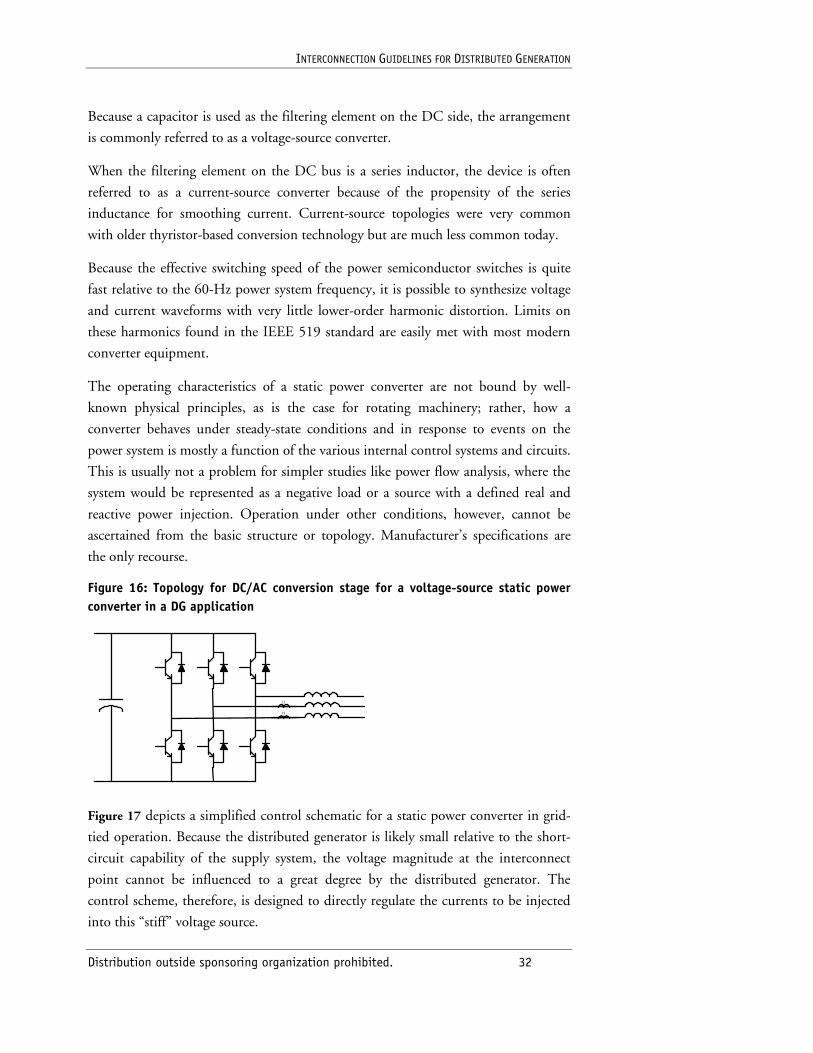
A common topology for DC/AC static power converters used in DG applications is
shown in Figure 16. The three-phase version of the system consists of six power
semiconductor switches, usually insulated-gate bipolar transistors (IGBTs) with an
integrated, reverse-paralleled diode. A capacitor on the DC link provides a small
amount of storage and serves as a filter to assist in smoothing the DC voltage. On the
AC side, inductors/reactors connect the three AC terminals of the switch matrix to
the power system. Small capacitive filters (not shown) are sometimes found on the
line side of the line interface reactors to remove noise generated by IGBT operation.
ac
dcac
dcPowerSystem
DGEnergySource
ac
dc
PowerSystem
DGEnergySource
INTERCONNECTION GUIDELINES FOR DISTRIBUTED GENERATION
Distribution outside sponsoring organization prohibited. 32
Because a capacitor is used as the filtering element on the DC side, the arrangement
is commonly referred to as a voltage-source converter.
When the filtering element on the DC bus is a series inductor, the device is often
referred to as a current-source converter because of the propensity of the series
inductance for smoothing current. Current-source topologies were very common
with older thyristor-based conversion technology but are much less common today.
Because the effective switching speed of the power semiconductor switches is quite
fast relative to the 60-Hz power system frequency, it is possible to synthesize voltage
and current waveforms with very little lower-order harmonic distortion. Limits on
these harmonics found in the IEEE 519 standard are easily met with most modern
converter equipment.
The operating characteristics of a static power converter are not bound by well-
known physical principles, as is the case for rotating machinery; rather, how a
converter behaves under steady-state conditions and in response to events on the
power system is mostly a function of the various internal control systems and circuits.
This is usually not a problem for simpler studies like power flow analysis, where the
system would be represented as a negative load or a source with a defined real and
reactive power injection. Operation under other conditions, however, cannot be
ascertained from the basic structure or topology. Manufacturer’s specifications are
the only recourse.
Figure 16: Topology for DC/AC conversion stage for a voltage-source static power converter in a DG application
Figure 17 depicts a simplified control schematic for a static power converter in grid-
tied operation. Because the distributed generator is likely small relative to the short-
circuit capability of the supply system, the voltage magnitude at the interconnect
point cannot be influenced to a great degree by the distributed generator. The
control scheme, therefore, is designed to directly regulate the currents to be injected
into this “stiff” voltage source.
I1
I1
INTERCONNECTION GUIDELINES FOR DISTRIBUTED GENERATION
Distribution outside sponsoring organization prohibited. 33
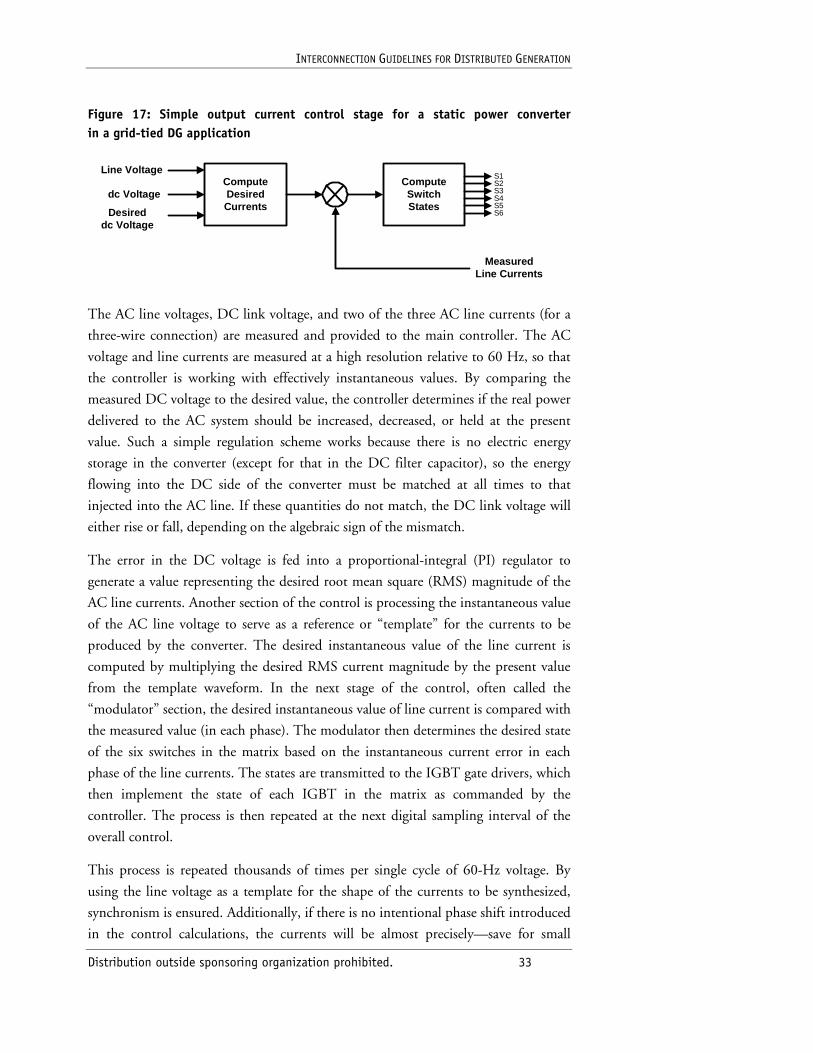
Figure 17: Simple output current control stage for a static power converter in a grid-tied DG application
The AC line voltages, DC link voltage, and two of the three AC line currents (for a
three-wire connection) are measured and provided to the main controller. The AC
voltage and line currents are measured at a high resolution relative to 60 Hz, so that
the controller is working with effectively instantaneous values. By comparing the
measured DC voltage to the desired value, the controller determines if the real power
delivered to the AC system should be increased, decreased, or held at the present
value. Such a simple regulation scheme works because there is no electric energy
storage in the converter (except for that in the DC filter capacitor), so the energy
flowing into the DC side of the converter must be matched at all times to that
injected into the AC line. If these quantities do not match, the DC link voltage will
either rise or fall, depending on the algebraic sign of the mismatch.
The error in the DC voltage is fed into a proportional-integral (PI) regulator to
generate a value representing the desired root mean square (RMS) magnitude of the
AC line currents. Another section of the control is processing the instantaneous value
of the AC line voltage to serve as a reference or “template” for the currents to be
produced by the converter. The desired instantaneous value of the line current is
computed by multiplying the desired RMS current magnitude by the present value
from the template waveform. In the next stage of the control, often called the
“modulator” section, the desired instantaneous value of line current is compared with
the measured value (in each phase). The modulator then determines the desired state
of the six switches in the matrix based on the instantaneous current error in each
phase of the line currents. The states are transmitted to the IGBT gate drivers, which
then implement the state of each IGBT in the matrix as commanded by the
controller. The process is then repeated at the next digital sampling interval of the
overall control.
This process is repeated thousands of times per single cycle of 60-Hz voltage. By
using the line voltage as a template for the shape of the currents to be synthesized,
synchronism is ensured. Additionally, if there is no intentional phase shift introduced
in the control calculations, the currents will be almost precisely—save for small
ComputeDesiredCurrents
ComputeSwitchStates
S1S2S3S4S5S6
Line Voltage
dc Voltage
Desireddc Voltage
MeasuredLine Currents
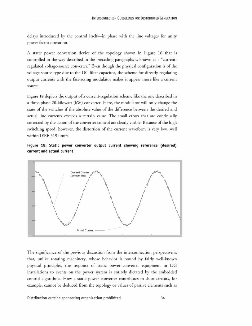
INTERCONNECTION GUIDELINES FOR DISTRIBUTED GENERATION
Distribution outside sponsoring organization prohibited. 34
delays introduced by the control itself—in phase with the line voltages for unity
power factor operation.
A static power conversion device of the topology shown in Figure 16 that is
controlled in the way described in the preceding paragraphs is known as a “current-
regulated voltage-source converter.” Even though the physical configuration is of the
voltage-source type due to the DC filter capacitor, the scheme for directly regulating
output currents with the fast-acting modulator makes it appear more like a current
source.
Figure 18 depicts the output of a current-regulation scheme like the one described in
a three-phase 20-kilowatt (kW) converter. Here, the modulator will only change the
state of the switches if the absolute value of the difference between the desired and
actual line currents exceeds a certain value. The small errors that are continually
corrected by the action of the converter control are clearly visible. Because of the high
switching speed, however, the distortion of the current waveform is very low, well
within IEEE 519 limits.
Figure 18: Static power converter output current showing reference (desired) current and actual current
The significance of the previous discussion from the interconnection perspective is
that, unlike rotating machinery, whose behavior is bound by fairly well-known
physical principles, the response of static power–converter equipment in DG
installations to events on the power system is entirely dictated by the embedded
control algorithms. How a static power converter contributes to short circuits, for
example, cannot be deduced from the topology or values of passive elements such as
-0.1
-0.06
-0.02
+0.02
+0.06
+0.1
Desired Current(smooth line)
Actual Current
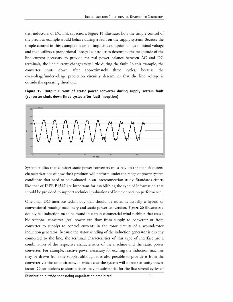
INTERCONNECTION GUIDELINES FOR DISTRIBUTED GENERATION
Distribution outside sponsoring organization prohibited. 35
ties, inductors, or DC link capacitors. Figure 19 illustrates how the simple control of
the previous example would behave during a fault on the supply system. Because the
simple control in this example makes an implicit assumption about nominal voltage
and then utilizes a proportional-integral controller to determine the magnitude of the
line current necessary to provide for real power balance between AC and DC
terminals, the line current changes very little during the fault. In this example, the
converter shuts down after approximately three cycles, because the
overvoltage/undervoltage protection circuitry determines that the line voltage is
outside the operating threshold.
Figure 19: Output current of static power converter during supply system fault (converter shuts down three cycles after fault inception)
System studies that consider static power converters must rely on the manufacturers’
characterizations of how their products will perform under the range of power system
conditions that need to be evaluated in an interconnection study. Standards efforts
like that of IEEE P1547 are important for establishing the type of information that
should be provided to support technical evaluations of interconnection performance.
One final DG interface technology that should be noted is actually a hybrid of
conventional rotating machinery and static power conversion. Figure 20 illustrates a
doubly fed induction machine found in certain commercial wind turbines that uses a
bidirectional converter (real power can flow from supply to converter or from
converter to supply) to control currents in the rotor circuits of a wound-rotor
induction generator. Because the stator winding of the induction generator is directly
connected to the line, the terminal characteristics of this type of interface are a
combination of the respective characteristics of the machine and the static power
converter. For example, reactive power necessary for exciting the induction machine
may be drawn from the supply, although it is also possible to provide it from the
converter via the rotor circuits, in which case the system will operate at unity power
factor. Contributions to short circuits may be substantial for the first several cycles of
Time (sec) 0.1 0.14 0.18 0.22 0.26 0.3
kA
-0.15
-0.1
-0.05
+0
+0.05
+0.1
+0.15Actual Current
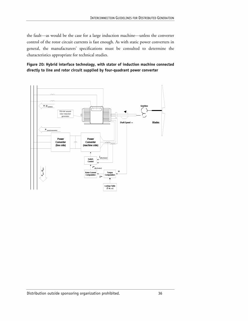
INTERCONNECTION GUIDELINES FOR DISTRIBUTED GENERATION
Distribution outside sponsoring organization prohibited. 36
the fault—as would be the case for a large induction machine—unless the converter
control of the rotor circuit currents is fast enough. As with static power converters in
general, the manufacturers’ specifications must be consulted to determine the
characteristics appropriate for technical studies.
Figure 20: Hybrid interface technology, with stator of induction machine connected directly to line and rotor circuit supplied by four-quadrant power converter
PowerConverter(line side)
PowerConverter
(machine side)
Pg
en ,Q
gen
P, Q (stator)
P (rotor/converter)
SwitchControl
TorqueComputation
Rotor CurrentComputation
Gearbox
750 kW wound-rotor induction
generator
i*abc(rotor)
iabc(rotor)
Lookup Table(T vs. Z)
Shaft Speed Z Blades
T*
Z
INTERCONNECTION GUIDELINES FOR DISTRIBUTED GENERATION
Distribution outside sponsoring organization prohibited. 37
4. Interconnection Requirements
This section focuses on interconnection requirements, including those detailed in the
draft of IEEE Standard P1547. The goal of this material is to provide additional
engineering background to allow for a better interpretation of the brief summaries of
requirements that appear in the standard. More detail is provided on such subjects as
islanding, detection of utility-side faults, and coordination with utility fault-clearing
and reclosing schemes. Additional information on protection of the distributed
resources (DR)/utility system interface is also provided.
4.1 General Protection Requirements
Because the distribution system was not designed for multiple sources of power, all
distributed resources must disconnect to allow the system fault-clearing process to
proceed. In most cases, the correct decisions about relaying for the DR breakers must
be made with only information available locally. This leads to questions such as
“How can DR relaying detect utility-side faults?” and “How should the relaying
coordinate with utility-side equipment?”
If the relaying does not properly detect disturbances on the utility side, the
distributed resources could end up isolated on a portion of the feeder load for times
ranging from a few cycles to several seconds. In some cases, the generation may
continue to feed the isolated section indefinitely. Regardless of time, this is referred
to as “islanding,” because it forms an electrical island that operates without
connection to the grid. Although there are some research efforts under way to
determine how to safely operate islands, or microgrids, most utilities currently forbid
the formation of inadvertent islands because of liability concerns. Therefore, another
important aspect of the protection issue that we address here is the detection of
islands.
There are at least three undesirable consequences of DR remaining connected for too
long after the utility breaker or line recloser has opened:
■ The fault fails to clear before the reclose operation. Arc products from temporary faults take several cycles to dissipate—time that is dependent on voltage level and climate. If the distributed resource continues to operate and feed the fault too long, there will be insufficient time to clear the fault, and the arc will restrike upon reclosing of the utility breaker. This will cause an unnecessary second operation of the breaker that can extend the scope of the interruption to more customers and subject utility transformers and lines to additional short-circuit currents.
■ The distributed resource is still connected when the utility breaker recloses. This can be devastating to some types of DR, particularly rotating machines. There is
INTERCONNECTION GUIDELINES FOR DISTRIBUTED GENERATION
Distribution outside sponsoring organization prohibited. 38
no guarantee that the reclosure will be in synchronism with the machine. The result can be very high winding forces and shaft torques due to out-of-phase energization. There might also be excessive breaker contact currents.
■ Frequency and voltage excursions can cause damage to load equipment.
We now examine the requirements related to these issues.
Detecting Utility-Side Faults
Ideally, DR relaying should detect a utility-side fault before the utility-side protective
equipment can operate, although this is not always possible. This is when it is easiest
to detect, because the voltages are likely to be abnormal while the fault is still present.
The primary means of fault detection will be abnormal voltages. The basic
functionality is to simply check the voltage magnitudes. The faulted phase would be
expected to be low due to the short circuit. Unfaulted phases may actually be higher
than normal.
The ability to recognize the voltage waveforms as being abnormal depends on the
transformer connection. Transformers with delta or ungrounded-wye primaries may
make it difficult to sense certain types of faults by voltage magnitude only from the
transformer secondary side. Negative-sequence voltage relaying can make the fault
detection more sensitive for these cases. Time delays on such relays should be at least
as long as for the voltage relays to avoid unnecessary generator trips for faults on
other feeders or for transient switching events (such as power factor correction
capacitors) that yield momentary imbalances.
Another problem is differentiating between faults on the feeder serving the DR and
faults on adjacent feeders or on the transmission system. Setting the DR relays too
sensitive will result in unnecessary tripping of the generation. One solution is to arm
the relay to trip when unusual voltages are detected but to delay tripping until utility
breakers would have normally had time to trip and clear the fault.
Transmission system breakers are fairly consistent in clearing faults in five to six
cycles. Clearing times of fault interrupters on distribution systems have much more
variation. Fuses can blow in as little as one-half cycle or take several seconds,
depending on the fault current magnitude. Mechanical interrupters such as breakers
or reclosers can operate in as short as 1.5 cycles but can also take a few seconds to
relay out on low-current faults. Once the trip signal occurs, the interruption would
be expected to take fewer than five cycles.
INTERCONNECTION GUIDELINES FOR DISTRIBUTED GENERATION
Distribution outside sponsoring organization prohibited. 39
Different delay times should be applied to different levels of over- or undervoltages
to reduce chances that the distributed resource is not disconnected inadvertently.
IEEE P1547 suggests two levels:
■ 0.16 seconds (s) (10 cycles) for voltages less than 50 percent. Very low voltages suggest that the fault is likely on the generator’s feeder or that the utility’s breaker has already opened, so the time delay can be short. However, it is also possible that there has been a major transmission fault or the fault is close to the substation bus on another feeder. The 10-cycle time delay is longer than the typical time for breakers to clear transmission and close-in faults (6 cycles) to prevent nuisance tripping, yet it is short enough to get the distributed resource off line early in the first reclose interval.
■ 2 s (120 cycles) for voltages between 50 percent and 88 percent. This condition would suggest that the fault is not close to the generator site and may be on an adjacent feeder or past a downstream line recloser or fuse. This delay gives the other fault interrupters an opportunity to clear the fault without tripping the generator off line.
For overvoltage relays, IEEE P1547 also recommends two levels:
■ 1.0 s for voltages between 110 percent and 120 percent.
■ 0.16 s for voltages greater than 120 percent.
Reverse power relaying would be applicable in DR installations where no net export
of power is expected (where customer load is always expected to be greater than the
generation). When a utility-side fault occurs, there may be a surge in power from the
generator back into the system that can be detected. Reverse power relays are
particularly useful for detecting islanding after the utility breaker opens.
Impedance relays may also be used to accomplish the same function as the reverse
power. These can be used to gain better detection of faults or detect the existence of
an island even when exported power is expected.
Overfrequency and underfrequency relays are not intended to be used for detecting
utility-side faults before the utility breaker opens. They are largely used for island
detection. However, field experience has indicated that generators are being
inadvertently tripped when utility-side faults occur by the frequency relays. The
reason claimed by relay manufacturers is that the relays are set to trip
instantaneously. Therefore, the voltage waveform disturbance that occurs upon fault
initiation is interpreted as a frequency change. Manufacturers suggest using at least a
six-cycle (0.1 s) time delay, which presumably gives the frequency detection
algorithm more time to compute the correct frequency.

INTERCONNECTION GUIDELINES FOR DISTRIBUTED GENERATION
Distribution outside sponsoring organization prohibited. 40
Coordinating with Utility Fault Clearing
Coordination is mainly a timing issue. The basic requirement for coordination with
utility fault-clearing practices is for the distributed resource to disconnect at the same
time the utility breaker operates or very soon thereafter. The generator is to be
disconnected from the system to allow the fault to clear, if possible, and to avoid
potential damage from reclosing out of phase.
The distributed resource must remain disconnected until system integrity has been
restored. IEEE P1547 requires the DR to remain off line until the voltage has
returned to normal for delays of up to 5 minutes, if the DR reconnection delay is
adjustable, or a fixed period of 5 minutes if fixed. Delays under 5 minutes will
typically require negotiation between the DR owner and the serving utility.
The tripping intelligence can come from either the utility-side fault-detection scheme
or the islanding-detection scheme. When local intelligence is insufficient, it will be
necessary to install direct transfer trip so that the interconnection breaker is operated
in concert with the main utility fault-interrupting device.
Islanding Detection
If the DR relaying has not detected a fault by the time the utility breaker opens, the
distributed resource is in an islanding condition, isolated on some or all of the feeder
load. Islanding detection must then pick up the fact that an island has occurred and
disconnect the DR before the utility system recloses. Islands may also occur without
faults when breakers are opened by operator error, equipment malfunction, or for
performing maintenance. There may be no danger of being exposed to a reclose in
that instance, but the islanding-detection scheme would be responsible for separating
the generator from the electric power system as promptly as possible.
Direct transfer trip is one sure way to coordinate the operation of the utility breaker
and the generator breaker. However, this is too costly for most DR systems
interconnected at the distribution level. The island must be detected by local
intelligence in these cases.
Basic island-detection functionality is provided by a combination of
overvoltage/undervoltage and overfrequency/underfrequency detection. If there is a
reactive power mismatch upon separation, the voltage excursion would generally be
quite noticeable. If the DR is producing more volt-amperes reactive (VARs) than the
system demands, the voltage will quickly rise to a new value, and vice-versa. Some
DR technologies do not produce reactive power while they are interconnected. If
there is no other source of reactive power, the system voltage will quickly collapse.
However, there are capacitors on most utility distribution feeders to help supply the
INTERCONNECTION GUIDELINES FOR DISTRIBUTED GENERATION
Distribution outside sponsoring organization prohibited. 41
reactive power. One strategy to prevent islands is to switch in a large reactive element
when the utility breaker opens to purposely create a large VAR mismatch. This
causes the voltage to immediately deviate from normal, and the island is detected by
the voltage relays on the distributed resource.
The island frequency would vary when there is a power mismatch. If there is too
much load, a rotating machine generator will slow down; too little, and the generator
speeds up, resulting in a corresponding frequency change. Inverters designed
according to IEEE Standard 929 introduce an intentional frequency error, or
periodically perturb their output current, in a manner that will tend to cause the
inverter output to quickly drift when they become islanded while controlled in grid-
connected mode.
The voltage relays will be set primarily to detect utility-side faults, with trip points as
described above.
Frequency relays should be set just outside the limits normally expected for utility
system frequency deviation and can be a very sensitive means of detecting an
inadvertent island. For DR less than 30 kilowatts (kW), IEEE P1547 recommends
setting the trip points at 59.3 hertz (Hz) for underfrequency and at 60.5 Hz for
overfrequency trip. Larger generation is permitted to stay on longer (unspecified time
delay) until the frequency drops below 57.0 Hz. The logic behind this standard is
that the larger generation might help prevent system collapse in an emergency. In any
case, whenever the frequency measured by the DR relay is outside the band allowed
for the utility, it is likely running islanded.
Some time delay should be used in the relay to ensure that an accurate measurement
of frequency is made. Otherwise, the overfrequency/underfrequency relaying can act
as a very sensitive fault detector and give false trips on common utility system
disturbances that temporarily alter the voltage waveshape. Manufacturers recommend
at least 0.1 s (six cycles). The IEEE P1547 document suggests 10 cycles, or 0.16 s.
It is generally expected that nearly all islands will be quickly detected by voltage and
frequency relays. In Electrotek’s own studies of this issue, less than 1 percent of
thousands of randomly generated cases of synchronous generator DR and load would
stay within both ±2 Hz and ±10 percent voltage for more than 1.0 s after a simple
opening of the utility feeder breaker. It was assumed that there was no fault on the
feeder and that the breaker opened while the system was normal. When a fault is
present before the opening, it is more likely the island will be detected early.
The problematic cases were where the DR output was slightly greater than the feeder
load. In cases where it is deemed more likely that the DR can sustain an island for at
INTERCONNECTION GUIDELINES FOR DISTRIBUTED GENERATION
Distribution outside sponsoring organization prohibited. 42
least the reclose period, basic protection can be supplemented by other islanding-
detection schemes:
■ Reverse power relaying is an obvious choice in systems that are not permitted to export power.
■ Impedance relays can be used for a similar function when export is permitted. The apparent impedance of the system will change, especially if the fault remains.
■ Instantaneous overvoltage detects conditions that result in distorted voltages, such as ferroresonant conditions that come about due to interaction between the distributed resource and capacitors on the system when the island forms.
Other, more exotic, schemes include these:
■ Harmonic voltage change. Harmonic currents normally flow through the utility source, causing minor voltage distortion. When the island forms, the short-circuit current increases considerably, causing the harmonic voltage distortion to increase.
■ Rate of change of power. This operates on the assumption that the distributed resource will suddenly attempt to export more power to match the load (this is dependent on generator and control technology).
One requirement consistent with IEEE P1547 is that interconnected distributed
resources should not attempt to regulate voltage but should control only power and
power factor. They should stay in this mode as long as the interconnection breaker is
closed. This significantly reduces the chances of forming a sustained island by
making it necessary to perfectly match active and reactive power of the entire system
to form an inadvertent island. In contrast, while running as a backup, stand-alone
power source, the generator must regulate voltage and frequency. It is much more
likely to sustain an island in that mode. This creates special multimode control
requirements for generators that operate in both grid-parallel and stand-alone modes.
4.2 Protection of the DR/EPS Interface
The specifications described here pertain only to protection of the DR/electrical
power system (EPS) interface and not necessarily to protection of the DR
technology. For example, synchronous generators are assumed to have the necessary
synchronizing relays and associated controls.
INTERCONNECTION GUIDELINES FOR DISTRIBUTED GENERATION
Distribution outside sponsoring organization prohibited. 43
Disconnect Switches
In addition to the protective relaying functions describe in subsequent sections, it is
nearly a universal requirement that DR installations of all sizes have disconnect
switches that can be locked out from areas that are accessible by utility personnel.
This is to prevent interconnection of the generator to the utility system during
certain maintenance operations or when system conditions do not permit
interconnection. An example of the latter would be when the DR site is being served
by an alternate feed that does not have the appropriate protection to accommodate
the generator.
Additional lock-out requirements could include in-facility transfer trip between all
breakers that can disconnect the distributed resource. This helps prevent conditions
in which the distributed resource might form an island inside the end-user facility
and accidentally reconnect out of synchronism.
In many cases, the disconnect switches will be required to have a visible open and
have load-break capability.
Simple Interconnection
The protection scheme shown in Figure 21 applies to small systems that are not
expected to be able to support islands. There is no consensus on what constitutes
“small” DR systems. The IEEE P1547/D08 document does not have a clear-cut
definition of size delineation, although that was attempted earlier in the standards
process. From Sections 4.2.1 and 4.2.2, one can infer that “small” would refer to DR
smaller than approximately 30 kW. Other utility interconnection standards might
restrict this to 10 kW or may allow this kind of interface protection up to 100 kW or
more.
DR of this size would commonly be connected to the load bus at secondary voltage
levels. Overcurrent protection is provided by molded case circuit breakers. The main
DR interface protection functions are overvoltage/undervoltage (27/59 relay) and
overfrequency/underfrequency (81 O/U relay).
These relays trip either the generator breaker or the main service breaker, depending
on the desired mode of operation. Tripping only the generator leaves the load
connected. If the DR is to be used as a backup power resource, the main service
breaker is tripped so that the generation can continue to supply the load. It should be
noted that special controls (not shown) may be required for this transfer to occur
seamlessly.
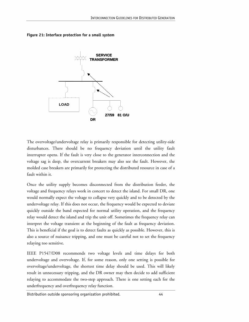
INTERCONNECTION GUIDELINES FOR DISTRIBUTED GENERATION
Distribution outside sponsoring organization prohibited. 44
Figure 21: Interface protection for a small system
The overvoltage/undervoltage relay is primarily responsible for detecting utility-side
disturbances. There should be no frequency deviation until the utility fault
interrupter opens. If the fault is very close to the generator interconnection and the
voltage sag is deep, the overcurrent breakers may also see the fault. However, the
molded case breakers are primarily for protecting the distributed resource in case of a
fault within it.
Once the utility supply becomes disconnected from the distribution feeder, the
voltage and frequency relays work in concert to detect the island. For small DR, one
would normally expect the voltage to collapse very quickly and to be detected by the
undervoltage relay. If this does not occur, the frequency would be expected to deviate
quickly outside the band expected for normal utility operation, and the frequency
relay would detect the island and trip the unit off. Sometimes the frequency relay can
interpret the voltage transient at the beginning of the fault as frequency deviation.
This is beneficial if the goal is to detect faults as quickly as possible. However, this is
also a source of nuisance tripping, and one must be careful not to set the frequency
relaying too sensitive.
IEEE P1547/D08 recommends two voltage levels and time delays for both
undervoltage and overvoltage. If, for some reason, only one setting is possible for
overvoltage/undervoltage, the shortest time delay should be used. This will likely
result in unnecessary tripping, and the DR owner may then decide to add sufficient
relaying to accommodate the two-step approach. There is one setting each for the
underfrequency and overfrequency relay function.
DR
LOAD
SERVICETRANSFORMER
81 O/U27/59DR
LOAD
SERVICETRANSFORMER
81 O/U27/59
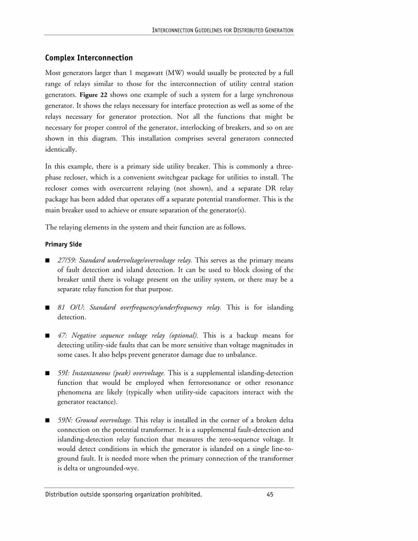
INTERCONNECTION GUIDELINES FOR DISTRIBUTED GENERATION
Distribution outside sponsoring organization prohibited. 45
Complex Interconnection
Most generators larger than 1 megawatt (MW) would usually be protected by a full
range of relays similar to those for the interconnection of utility central station
generators. Figure 22 shows one example of such a system for a large synchronous
generator. It shows the relays necessary for interface protection as well as some of the
relays necessary for generator protection. Not all the functions that might be
necessary for proper control of the generator, interlocking of breakers, and so on are
shown in this diagram. This installation comprises several generators connected
identically.
In this example, there is a primary side utility breaker. This is commonly a three-
phase recloser, which is a convenient switchgear package for utilities to install. The
recloser comes with overcurrent relaying (not shown), and a separate DR relay
package has been added that operates off a separate potential transformer. This is the
main breaker used to achieve or ensure separation of the generator(s).
The relaying elements in the system and their function are as follows.
Primary Side
■ 27/59: Standard undervoltage/overvoltage relay. This serves as the primary means of fault detection and island detection. It can be used to block closing of the breaker until there is voltage present on the utility system, or there may be a separate relay function for that purpose.
■ 81 O/U: Standard overfrequency/underfrequency relay. This is for islanding detection.
■ 47: Negative sequence voltage relay (optional). This is a backup means for detecting utility-side faults that can be more sensitive than voltage magnitudes in some cases. It also helps prevent generator damage due to unbalance.
■ 59I: Instantaneous (peak) overvoltage. This is a supplemental islanding-detection function that would be employed when ferroresonance or other resonance phenomena are likely (typically when utility-side capacitors interact with the generator reactance).
■ 59N: Ground overvoltage. This relay is installed in the corner of a broken delta connection on the potential transformer. It is a supplemental fault-detection and islanding-detection relay function that measures the zero-sequence voltage. It would detect conditions in which the generator is islanded on a single line-to-ground fault. It is needed more when the primary connection of the transformer is delta or ungrounded-wye.
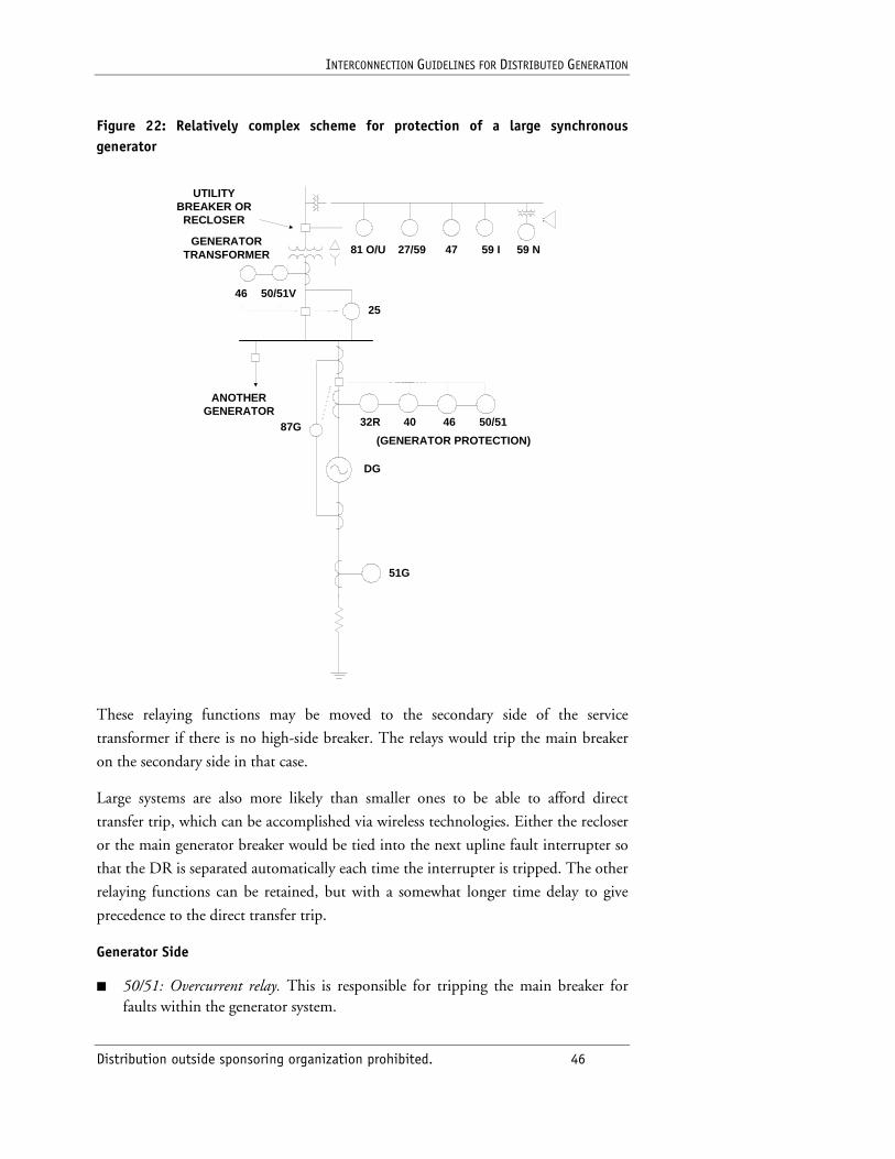
INTERCONNECTION GUIDELINES FOR DISTRIBUTED GENERATION
Distribution outside sponsoring organization prohibited. 46
Figure 22: Relatively complex scheme for protection of a large synchronous generator
These relaying functions may be moved to the secondary side of the service
transformer if there is no high-side breaker. The relays would trip the main breaker
on the secondary side in that case.
Large systems are also more likely than smaller ones to be able to afford direct
transfer trip, which can be accomplished via wireless technologies. Either the recloser
or the main generator breaker would be tied into the next upline fault interrupter so
that the DR is separated automatically each time the interrupter is tripped. The other
relaying functions can be retained, but with a somewhat longer time delay to give
precedence to the direct transfer trip.
Generator Side
■ 50/51: Overcurrent relay. This is responsible for tripping the main breaker for faults within the generator system.
DG
ANOTHERGENERATOR
GENERATORTRANSFORMER 81 O/U 47 59 I
25
50/51V46
50/51464032R
(GENERATOR PROTECTION)
51G
87G
UTILITYBREAKER OR
RECLOSER
59 N27/59
INTERCONNECTION GUIDELINES FOR DISTRIBUTED GENERATION
Distribution outside sponsoring organization prohibited. 47
■ 46 relay at transformer: Negative sequence current. Used particularly in open-phase conditions and trips the main breaker. (Generators have a separate 46 relay.)
■ 25: Synchronizing relay. This controls closing of the main breaker when the generator(s) are being interconnected to the utility. (This scheme would also require synch check relays on the individual generators if they are to be interconnected separately.)
Generator Protection
■ 87G: Differential ground relay. Used for fast detection of ground faults within the generator.
■ 51G: Ground overcurrent. Trips the generator for high neutral currents indicative of a ground fault on the secondary system.
■ 32R: Reverse power relay. This relay detects power going into the generator, which would indicate a fault.
■ 40: Loss of field relay. Detects loss of field excitation.
■ 46: Negative sequence current. Protects the machine against excessive unbalanced currents, which may or may not result from a fault.
■ 50/51: Overcurrent relays. Protect the generator against excessive loads and faults on either side of the generator breaker.
This example demonstrates the majority of relaying functions that would be used to
interconnect distributed resources to the utility distribution system. Many of these
functions can be obtained from special DR interface relay packages that can be
conveniently installed. The package that controls the interface breakers is generally
required to be “utility grade.” Generator protection relays typically are supplied with
the generator.
Other Interconnection Schemes
The protection schemes presented represent just two of the many possible
arrangements. In fact, documents as large as this guide have been written on this
subject alone. These two schemes were presented to show the range of protective
relaying requirements for interconnecting DR to the utility system. The schemes
presented here also focus on the interface protection. In any given DR system, there
may be many other relays and interlocks associated with the control of the system.
C.J. Mozina3 gives several other examples. Also, there are extensive documents
available on the Web sites of the major vendors of generation protection relays.4
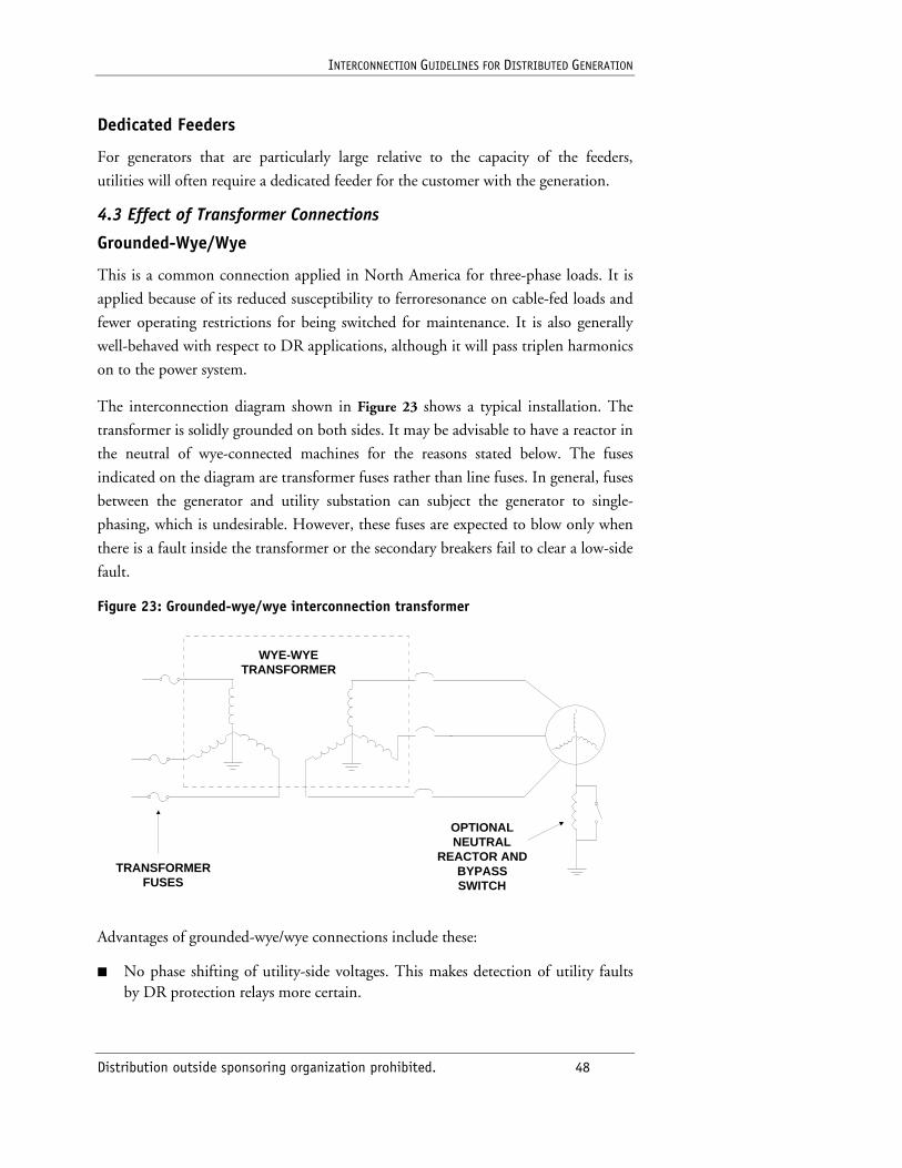
INTERCONNECTION GUIDELINES FOR DISTRIBUTED GENERATION
Distribution outside sponsoring organization prohibited. 48
Dedicated Feeders
For generators that are particularly large relative to the capacity of the feeders,
utilities will often require a dedicated feeder for the customer with the generation.
4.3 Effect of Transformer Connections
Grounded-Wye/Wye
This is a common connection applied in North America for three-phase loads. It is
applied because of its reduced susceptibility to ferroresonance on cable-fed loads and
fewer operating restrictions for being switched for maintenance. It is also generally
well-behaved with respect to DR applications, although it will pass triplen harmonics
on to the power system.
The interconnection diagram shown in Figure 23 shows a typical installation. The
transformer is solidly grounded on both sides. It may be advisable to have a reactor in
the neutral of wye-connected machines for the reasons stated below. The fuses
indicated on the diagram are transformer fuses rather than line fuses. In general, fuses
between the generator and utility substation can subject the generator to single-
phasing, which is undesirable. However, these fuses are expected to blow only when
there is a fault inside the transformer or the secondary breakers fail to clear a low-side
fault.
Figure 23: Grounded-wye/wye interconnection transformer
TRANSFORMERFUSES
OPTIONALNEUTRAL
REACTOR ANDBYPASSSWITCH
WYE-WYETRANSFORMER
Advantages of grounded-wye/wye connections include these:
■ No phase shifting of utility-side voltages. This makes detection of utility faults by DR protection relays more certain.
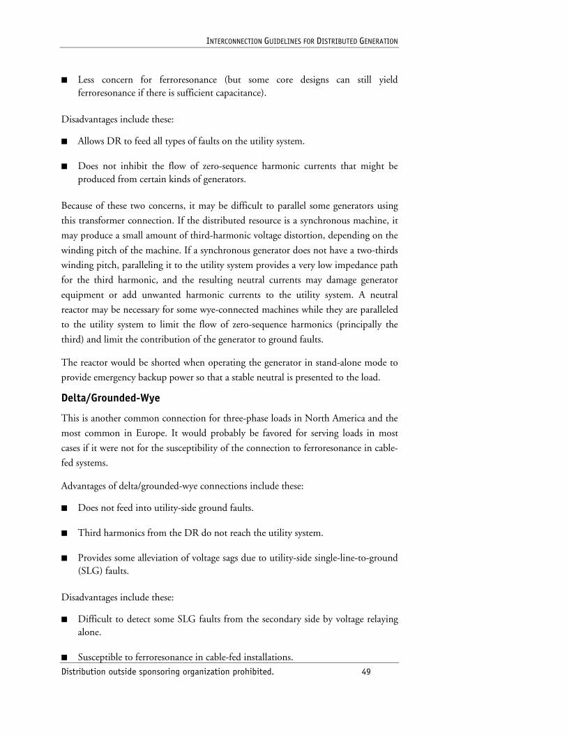
INTERCONNECTION GUIDELINES FOR DISTRIBUTED GENERATION
Distribution outside sponsoring organization prohibited. 49
■ Less concern for ferroresonance (but some core designs can still yield ferroresonance if there is sufficient capacitance).
Disadvantages include these:
■ Allows DR to feed all types of faults on the utility system.
■ Does not inhibit the flow of zero-sequence harmonic currents that might be produced from certain kinds of generators.
Because of these two concerns, it may be difficult to parallel some generators using
this transformer connection. If the distributed resource is a synchronous machine, it
may produce a small amount of third-harmonic voltage distortion, depending on the
winding pitch of the machine. If a synchronous generator does not have a two-thirds
winding pitch, paralleling it to the utility system provides a very low impedance path
for the third harmonic, and the resulting neutral currents may damage generator
equipment or add unwanted harmonic currents to the utility system. A neutral
reactor may be necessary for some wye-connected machines while they are paralleled
to the utility system to limit the flow of zero-sequence harmonics (principally the
third) and limit the contribution of the generator to ground faults.
The reactor would be shorted when operating the generator in stand-alone mode to
provide emergency backup power so that a stable neutral is presented to the load.
Delta/Grounded-Wye
This is another common connection for three-phase loads in North America and the
most common in Europe. It would probably be favored for serving loads in most
cases if it were not for the susceptibility of the connection to ferroresonance in cable-
fed systems.
Advantages of delta/grounded-wye connections include these:
■ Does not feed into utility-side ground faults.
■ Third harmonics from the DR do not reach the utility system.
■ Provides some alleviation of voltage sags due to utility-side single-line-to-ground (SLG) faults.
Disadvantages include these:
■ Difficult to detect some SLG faults from the secondary side by voltage relaying alone.
■ Susceptible to ferroresonance in cable-fed installations.
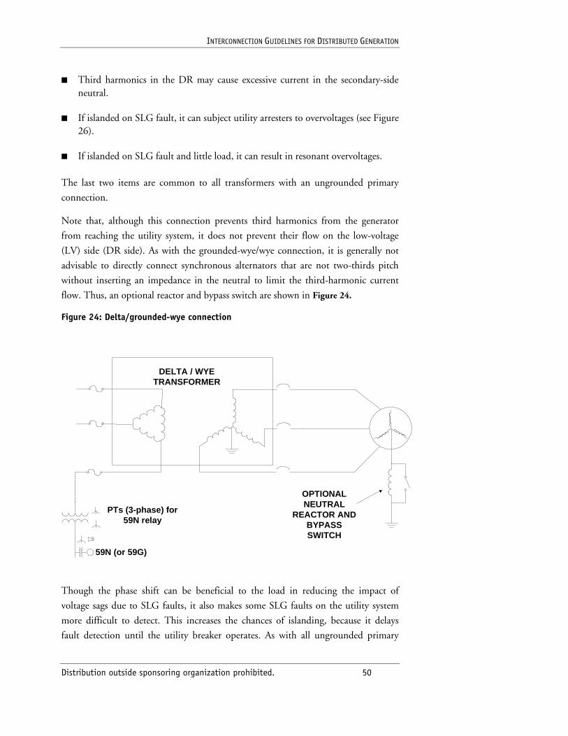
INTERCONNECTION GUIDELINES FOR DISTRIBUTED GENERATION
Distribution outside sponsoring organization prohibited. 50
■ Third harmonics in the DR may cause excessive current in the secondary-side neutral.
■ If islanded on SLG fault, it can subject utility arresters to overvoltages (see Figure 26).
■ If islanded on SLG fault and little load, it can result in resonant overvoltages.
The last two items are common to all transformers with an ungrounded primary
connection.
Note that, although this connection prevents third harmonics from the generator
from reaching the utility system, it does not prevent their flow on the low-voltage
(LV) side (DR side). As with the grounded-wye/wye connection, it is generally not
advisable to directly connect synchronous alternators that are not two-thirds pitch
without inserting an impedance in the neutral to limit the third-harmonic current
flow. Thus, an optional reactor and bypass switch are shown in Figure 24.
Figure 24: Delta/grounded-wye connection�
Though the phase shift can be beneficial to the load in reducing the impact of
voltage sags due to SLG faults, it also makes some SLG faults on the utility system
more difficult to detect. This increases the chances of islanding, because it delays
fault detection until the utility breaker operates. As with all ungrounded primary
OPTIONALNEUTRAL
REACTOR ANDBYPASSSWITCH
DELTA / WYETRANSFORMER
PTs (3-phase) for59N relay
59N (or 59G)
INTERCONNECTION GUIDELINES FOR DISTRIBUTED GENERATION
Distribution outside sponsoring organization prohibited. 51
connections, there is a danger in being islanded on an SLG fault with very light load
even briefly, because this can result in a resonant condition.
Therefore, it is common to add other relaying functions to aid in the early detection
of utility-side faults. A negative sequence relay can make the detection more reliable.
Though the voltage magnitudes seen on the secondary may not change sufficiently,
they will become unbalanced, resulting in detectable negative sequence voltages and
currents.
A common approach is to add relaying on the primary side of the transformer, such
as a ground overvoltage (59N or 59G in Figure 24) relay that can detect the presence
of the SLG fault. This is implemented by installing potential transformers on the
primary system and then placing a voltage relay in the corner of the delta winding on
the instrumentation transformer.
Grounded-Wye/Delta
Some utility engineers claim that grounded-wye/delta is the best connection for DR.
In fact, it is the most common connection used for most utility central station
generation and large merchant plants directly connected to the transmission system.
Advantages of grounded-wye/delta connections include these:
■ Protection schemes are well understood by both vendors of larger DR equipment and utility protection engineers.
■ Third-harmonic currents that might be produced by the generator cannot flow on the generator side and are, therefore, not passed on to the power system. Thus, economies in generator design might be realizable, and no neutral reactor is necessary to limit the current.
■ On the distribution system, utility-side faults make themselves known on the DR side quite readily, because the transformer itself actually participates in all ground faults. (This connection is also known as a “grounding transformer” or a “ground source.”)
Unfortunately, this behavior of participating in all ground faults is undesirable on
many distribution systems, and few utilities will allow this connection on the
distribution system without special study. Accepting this connection often means
making changes to the feeder overcurrent protection scheme that are either costly in
terms of replacing equipment or that inconvenience other customers on the feeder.
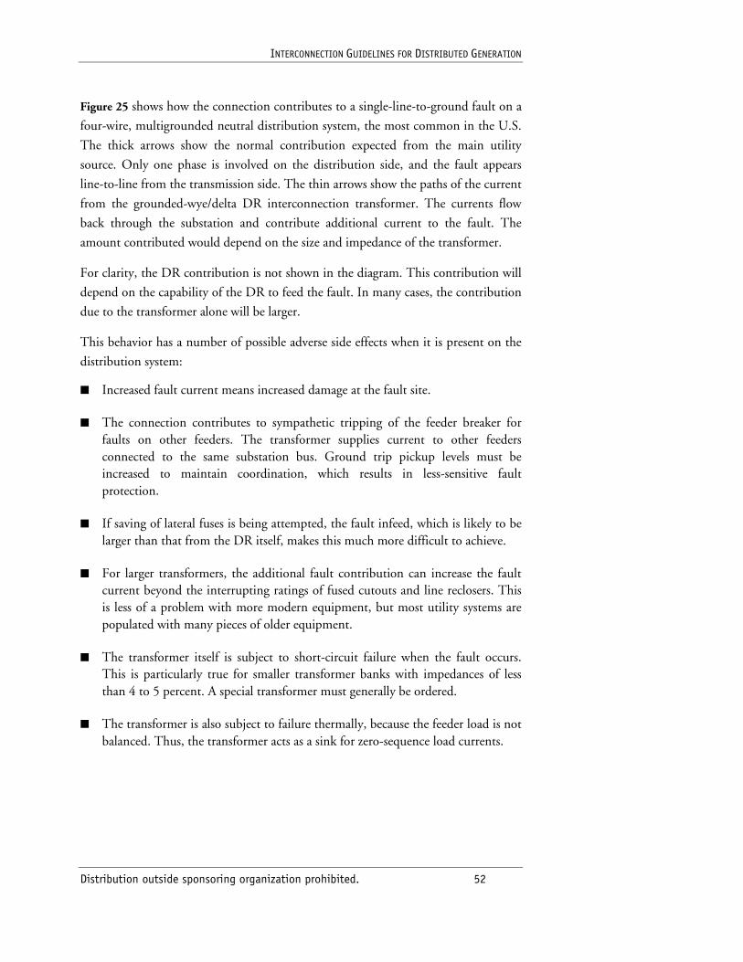
INTERCONNECTION GUIDELINES FOR DISTRIBUTED GENERATION
Distribution outside sponsoring organization prohibited. 52
Figure 25 shows how the connection contributes to a single-line-to-ground fault on a
four-wire, multigrounded neutral distribution system, the most common in the U.S.
The thick arrows show the normal contribution expected from the main utility
source. Only one phase is involved on the distribution side, and the fault appears
line-to-line from the transmission side. The thin arrows show the paths of the current
from the grounded-wye/delta DR interconnection transformer. The currents flow
back through the substation and contribute additional current to the fault. The
amount contributed would depend on the size and impedance of the transformer.
For clarity, the DR contribution is not shown in the diagram. This contribution will
depend on the capability of the DR to feed the fault. In many cases, the contribution
due to the transformer alone will be larger.
This behavior has a number of possible adverse side effects when it is present on the
distribution system:
■ Increased fault current means increased damage at the fault site.
■ The connection contributes to sympathetic tripping of the feeder breaker for faults on other feeders. The transformer supplies current to other feeders connected to the same substation bus. Ground trip pickup levels must be increased to maintain coordination, which results in less-sensitive fault protection.
■ If saving of lateral fuses is being attempted, the fault infeed, which is likely to be larger than that from the DR itself, makes this much more difficult to achieve.
■ For larger transformers, the additional fault contribution can increase the fault current beyond the interrupting ratings of fused cutouts and line reclosers. This is less of a problem with more modern equipment, but most utility systems are populated with many pieces of older equipment.
■ The transformer itself is subject to short-circuit failure when the fault occurs. This is particularly true for smaller transformer banks with impedances of less than 4 to 5 percent. A special transformer must generally be ordered.
■ The transformer is also subject to failure thermally, because the feeder load is not balanced. Thus, the transformer acts as a sink for zero-sequence load currents.
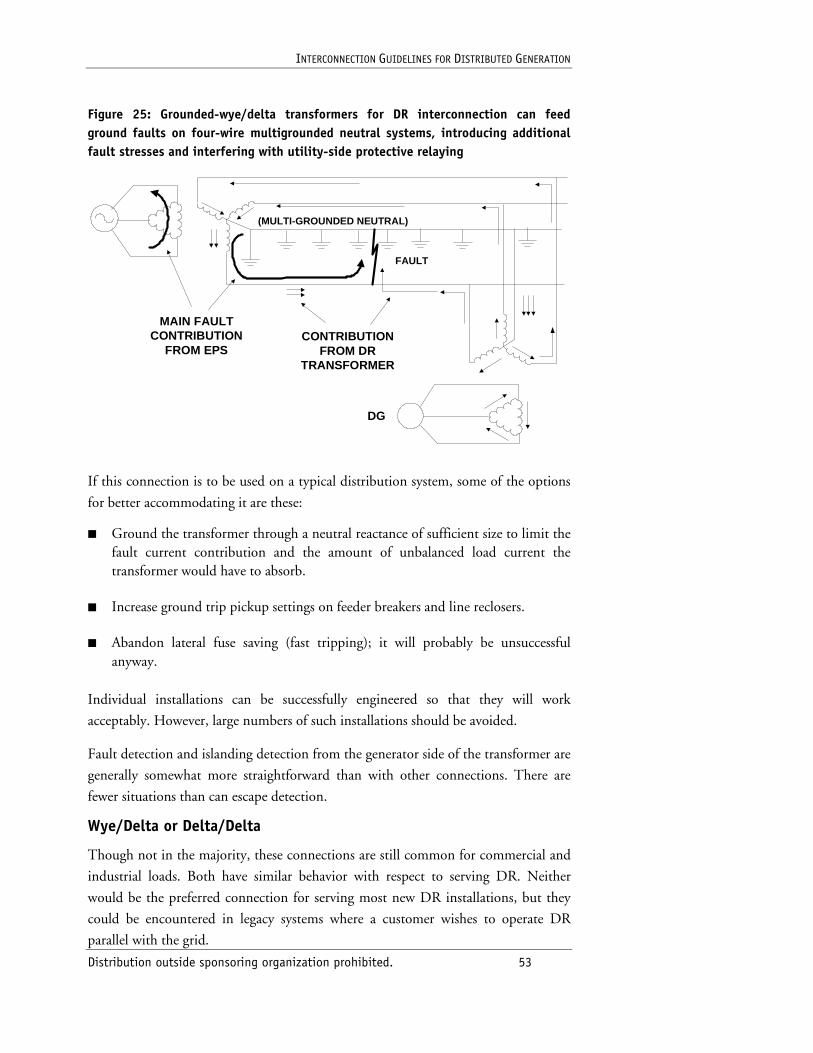
INTERCONNECTION GUIDELINES FOR DISTRIBUTED GENERATION
Distribution outside sponsoring organization prohibited. 53
Figure 25: Grounded-wye/delta transformers for DR interconnection can feed ground faults on four-wire multigrounded neutral systems, introducing additional fault stresses and interfering with utility-side protective relaying
MAIN FAULTCONTRIBUTION
FROM EPSCONTRIBUTION
FROM DRTRANSFORMER
(MULTI-GROUNDED NEUTRAL)
FAULT
DG
If this connection is to be used on a typical distribution system, some of the options
for better accommodating it are these:
■ Ground the transformer through a neutral reactance of sufficient size to limit the fault current contribution and the amount of unbalanced load current the transformer would have to absorb.
■ Increase ground trip pickup settings on feeder breakers and line reclosers.
■ Abandon lateral fuse saving (fast tripping); it will probably be unsuccessful anyway.
Individual installations can be successfully engineered so that they will work
acceptably. However, large numbers of such installations should be avoided.
Fault detection and islanding detection from the generator side of the transformer are
generally somewhat more straightforward than with other connections. There are
fewer situations than can escape detection.
Wye/Delta or Delta/Delta
Though not in the majority, these connections are still common for commercial and
industrial loads. Both have similar behavior with respect to serving DR. Neither
would be the preferred connection for serving most new DR installations, but they
could be encountered in legacy systems where a customer wishes to operate DR
parallel with the grid.
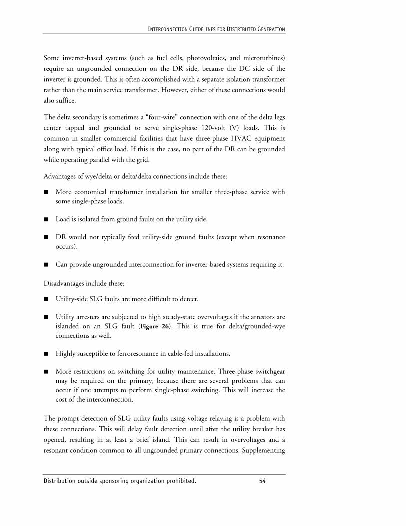
INTERCONNECTION GUIDELINES FOR DISTRIBUTED GENERATION
Distribution outside sponsoring organization prohibited. 54
Some inverter-based systems (such as fuel cells, photovoltaics, and microturbines)
require an ungrounded connection on the DR side, because the DC side of the
inverter is grounded. This is often accomplished with a separate isolation transformer
rather than the main service transformer. However, either of these connections would
also suffice.
The delta secondary is sometimes a “four-wire” connection with one of the delta legs
center tapped and grounded to serve single-phase 120-volt (V) loads. This is
common in smaller commercial facilities that have three-phase HVAC equipment
along with typical office load. If this is the case, no part of the DR can be grounded
while operating parallel with the grid.
Advantages of wye/delta or delta/delta connections include these:
■ More economical transformer installation for smaller three-phase service with some single-phase loads.
■ Load is isolated from ground faults on the utility side.
■ DR would not typically feed utility-side ground faults (except when resonance occurs).
■ Can provide ungrounded interconnection for inverter-based systems requiring it.
Disadvantages include these:
■ Utility-side SLG faults are more difficult to detect.
■ Utility arresters are subjected to high steady-state overvoltages if the arrestors are islanded on an SLG fault (Figure 26). This is true for delta/grounded-wye connections as well.
■ Highly susceptible to ferroresonance in cable-fed installations.
■ More restrictions on switching for utility maintenance. Three-phase switchgear may be required on the primary, because there are several problems that can occur if one attempts to perform single-phase switching. This will increase the cost of the interconnection.
The prompt detection of SLG utility faults using voltage relaying is a problem with
these connections. This will delay fault detection until after the utility breaker has
opened, resulting in at least a brief island. This can result in overvoltages and a
resonant condition common to all ungrounded primary connections. Supplementing
INTERCONNECTION GUIDELINES FOR DISTRIBUTED GENERATION
Distribution outside sponsoring organization prohibited. 55
voltage relaying with negative sequence current or voltage relaying can make the
detection more certain.
Figure 26: Transformers with ungrounded primary connections can subject utility-side arresters to overvoltage
ARRESTERSSUBJECTED TO LINE-TO-LINE VOLTAGES
PERMANENT LINE-TO-GROUND FAULT
UTILITYINTERRUPTINGDEVICE OPEN
UNGROUNDEDTRANSFORMERCONNECTION
G
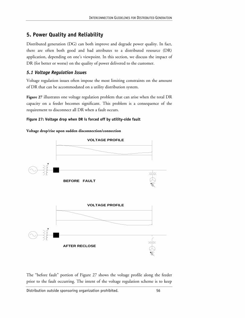
INTERCONNECTION GUIDELINES FOR DISTRIBUTED GENERATION
Distribution outside sponsoring organization prohibited. 56
5. Power Quality and Reliability
Distributed generation (DG) can both improve and degrade power quality. In fact,
there are often both good and bad attributes to a distributed resource (DR)
application, depending on one’s viewpoint. In this section, we discuss the impact of
DR (for better or worse) on the quality of power delivered to the customer.
5.1 Voltage Regulation Issues
Voltage regulation issues often impose the most limiting constraints on the amount
of DR that can be accommodated on a utility distribution system.
Figure 27 illustrates one voltage regulation problem that can arise when the total DR
capacity on a feeder becomes significant. This problem is a consequence of the
requirement to disconnect all DR when a fault occurs.
Figure 27: Voltage drop when DR is forced off by utility-side fault
Voltage drop/rise upon sudden disconnection/connection
The “before fault” portion of Figure 27 shows the voltage profile along the feeder
prior to the fault occurring. The intent of the voltage regulation scheme is to keep
VOLTAGE PROFILE
BEFORE FAULT
VOLTAGE PROFILE
AFTER RECLOSE
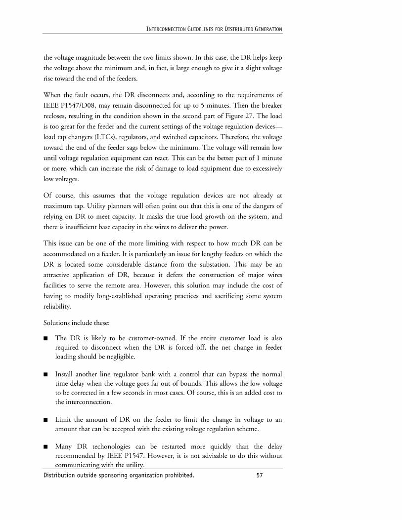
INTERCONNECTION GUIDELINES FOR DISTRIBUTED GENERATION
Distribution outside sponsoring organization prohibited. 57
the voltage magnitude between the two limits shown. In this case, the DR helps keep
the voltage above the minimum and, in fact, is large enough to give it a slight voltage
rise toward the end of the feeders.
When the fault occurs, the DR disconnects and, according to the requirements of
IEEE P1547/D08, may remain disconnected for up to 5 minutes. Then the breaker
recloses, resulting in the condition shown in the second part of Figure 27. The load
is too great for the feeder and the current settings of the voltage regulation devices—
load tap changers (LTCs), regulators, and switched capacitors. Therefore, the voltage
toward the end of the feeder sags below the minimum. The voltage will remain low
until voltage regulation equipment can react. This can be the better part of 1 minute
or more, which can increase the risk of damage to load equipment due to excessively
low voltages.
Of course, this assumes that the voltage regulation devices are not already at
maximum tap. Utility planners will often point out that this is one of the dangers of
relying on DR to meet capacity. It masks the true load growth on the system, and
there is insufficient base capacity in the wires to deliver the power.
This issue can be one of the more limiting with respect to how much DR can be
accommodated on a feeder. It is particularly an issue for lengthy feeders on which the
DR is located some considerable distance from the substation. This may be an
attractive application of DR, because it defers the construction of major wires
facilities to serve the remote area. However, this solution may include the cost of
having to modify long-established operating practices and sacrificing some system
reliability.
Solutions include these:
■ The DR is likely to be customer-owned. If the entire customer load is also required to disconnect when the DR is forced off, the net change in feeder loading should be negligible.
■ Install another line regulator bank with a control that can bypass the normal time delay when the voltage goes far out of bounds. This allows the low voltage to be corrected in a few seconds in most cases. Of course, this is an added cost to the interconnection.
■ Limit the amount of DR on the feeder to limit the change in voltage to an amount that can be accepted with the existing voltage regulation scheme.
■ Many DR techonologies can be restarted more quickly than the delay recommended by IEEE P1547. However, it is not advisable to do this without communicating with the utility.
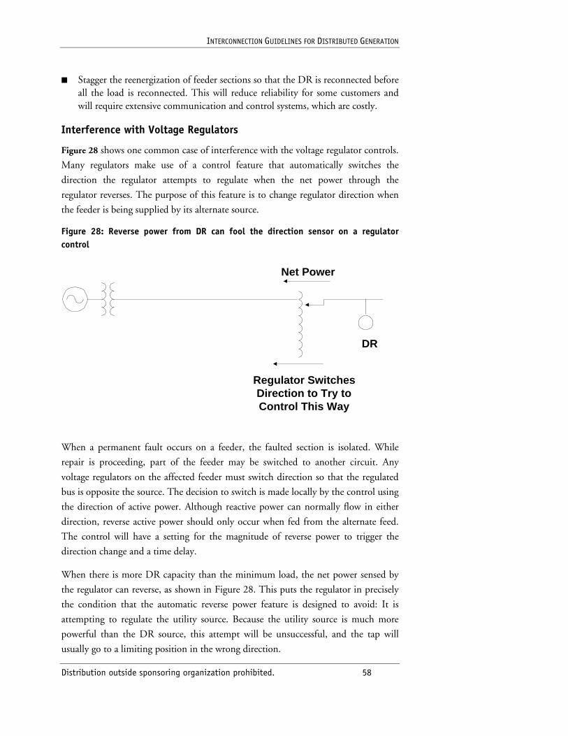
INTERCONNECTION GUIDELINES FOR DISTRIBUTED GENERATION
Distribution outside sponsoring organization prohibited. 58
■ Stagger the reenergization of feeder sections so that the DR is reconnected before all the load is reconnected. This will reduce reliability for some customers and will require extensive communication and control systems, which are costly.
Interference with Voltage Regulators
Figure 28 shows one common case of interference with the voltage regulator controls.
Many regulators make use of a control feature that automatically switches the
direction the regulator attempts to regulate when the net power through the
regulator reverses. The purpose of this feature is to change regulator direction when
the feeder is being supplied by its alternate source.
Figure 28: Reverse power from DR can fool the direction sensor on a regulator control
When a permanent fault occurs on a feeder, the faulted section is isolated. While
repair is proceeding, part of the feeder may be switched to another circuit. Any
voltage regulators on the affected feeder must switch direction so that the regulated
bus is opposite the source. The decision to switch is made locally by the control using
the direction of active power. Although reactive power can normally flow in either
direction, reverse active power should only occur when fed from the alternate feed.
The control will have a setting for the magnitude of reverse power to trigger the
direction change and a time delay.
When there is more DR capacity than the minimum load, the net power sensed by
the regulator can reverse, as shown in Figure 28. This puts the regulator in precisely
the condition that the automatic reverse power feature is designed to avoid: It is
attempting to regulate the utility source. Because the utility source is much more
powerful than the DR source, this attempt will be unsuccessful, and the tap will
usually go to a limiting position in the wrong direction.
DR
Regulator SwitchesDirection to Try toControl This Way
Net Power
INTERCONNECTION GUIDELINES FOR DISTRIBUTED GENERATION
Distribution outside sponsoring organization prohibited. 59
The regulator should stay in the normal forward control mode in this condition.
Solutions to this problem include these:
■ Some microprocessor-based regulator controls have a “cogeneration” mode that prevents reversing when the generator is interconnected. Reverse power may alter the control strategy but does not change the direction. For DR that is operating most of the time, the control can simply be left in this mode. For intermittent generation, operation would be improved if there were communications circuits available to coordinate the actions of the DR and the control.
■ Set the control to go to neutral tap on reverse power. This can minimize the impacts of incorrect voltage regulator action, although it will not provide good voltage regulation when the feeder is actually being fed from the alternate circuit.
■ Replace older-generation, simpler regulator controls with those that have cogeneration and communications features.
■ Move the regulator back toward the substation so that there is more load on the DR side of the regulator.
■ Limit the DR output.
Varying Generation
Varying generation can also cause problems for utility voltage regulation equipment.
Much of the DR for which interconnection is contemplated will not be varying.
When the energy source is fossil fuel, the DR will typically be operated at full output
all the time it is connected. Variable sources are largely renewable sources such as
solar and wind generation. Wind generation is typically the more difficult to deal
with, because it can vary greatly in a matter of seconds—much faster than standard
utility voltage regulation equipment can respond.
A proposed wind farm installation is shown in Figure 29. An 8,000-kilowatt (kW)
wind farm was to be located nearly 7.5 miles from the substation on a 12.47-kilovolt
(kV) feeder. This is a very large flow for this class of feeder. The conductor in the
main three-phase feeder was 336 MCM ACSR constructed on a typical 8-foot
horizontal crossarm and was not transposed over its entire length. The voltage- and
volt-ampere reactive (VAR)-control devices consisted of two 600-kVAR switch
capacitor banks and a line regulator positioned as shown in Figure 29. The capacitor
switches were controlled by current magnitude. The voltage regulator was set for 122
volts (V) and a bandwidth of 3 V.
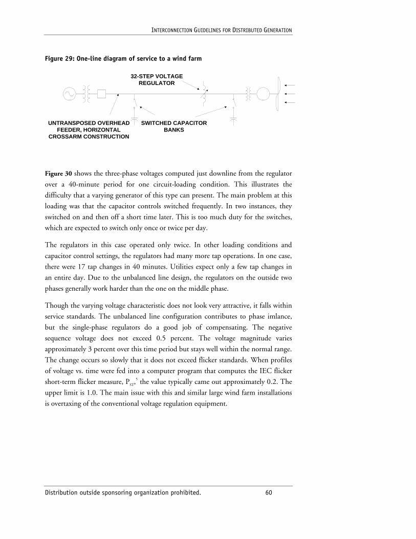
INTERCONNECTION GUIDELINES FOR DISTRIBUTED GENERATION
Distribution outside sponsoring organization prohibited. 60
Figure 29: One-line diagram of service to a wind farm
SWITCHED CAPACITORBANKS
32-STEP VOLTAGEREGULATOR
UNTRANSPOSED OVERHEADFEEDER, HORIZONTAL
CROSSARM CONSTRUCTION
Figure 30 shows the three-phase voltages computed just downline from the regulator
over a 40-minute period for one circuit-loading condition. This illustrates the
difficulty that a varying generator of this type can present. The main problem at this
loading was that the capacitor controls switched frequently. In two instances, they
switched on and then off a short time later. This is too much duty for the switches,
which are expected to switch only once or twice per day.
The regulators in this case operated only twice. In other loading conditions and
capacitor control settings, the regulators had many more tap operations. In one case,
there were 17 tap changes in 40 minutes. Utilities expect only a few tap changes in
an entire day. Due to the unbalanced line design, the regulators on the outside two
phases generally work harder than the one on the middle phase.
Though the varying voltage characteristic does not look very attractive, it falls within
service standards. The unbalanced line configuration contributes to phase imlance,
but the single-phase regulators do a good job of compensating. The negative
sequence voltage does not exceed 0.5 percent. The voltage magnitude varies
approximately 3 percent over this time period but stays well within the normal range.
The change occurs so slowly that it does not exceed flicker standards. When profiles
of voltage vs. time were fed into a computer program that computes the IEC flicker
short-term flicker measure, PST,5 the value typically came out approximately 0.2. The
upper limit is 1.0. The main issue with this and similar large wind farm installations
is overtaxing of the conventional voltage regulation equipment.
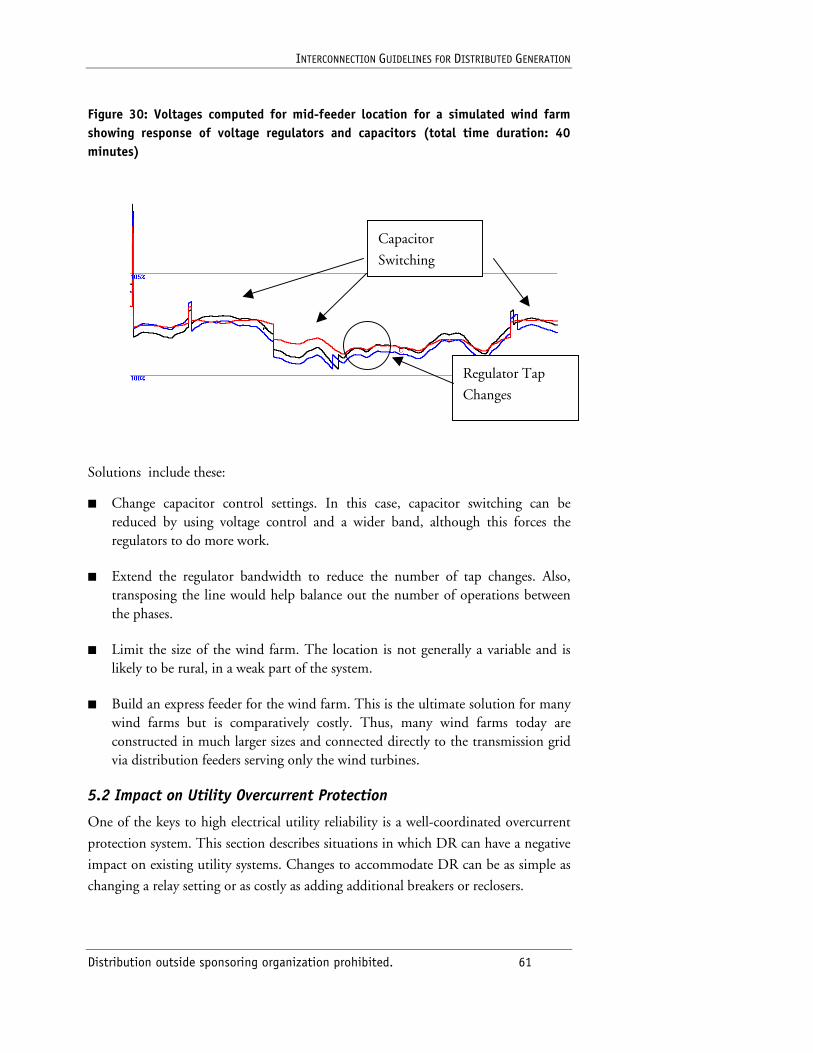
INTERCONNECTION GUIDELINES FOR DISTRIBUTED GENERATION
Distribution outside sponsoring organization prohibited. 61
Figure 30: Voltages computed for mid-feeder location for a simulated wind farm showing response of voltage regulators and capacitors (total time duration: 40 minutes)
Solutions include these:
■ Change capacitor control settings. In this case, capacitor switching can be reduced by using voltage control and a wider band, although this forces the regulators to do more work.
■ Extend the regulator bandwidth to reduce the number of tap changes. Also, transposing the line would help balance out the number of operations between the phases.
■ Limit the size of the wind farm. The location is not generally a variable and is likely to be rural, in a weak part of the system.
■ Build an express feeder for the wind farm. This is the ultimate solution for many wind farms but is comparatively costly. Thus, many wind farms today are constructed in much larger sizes and connected directly to the transmission grid via distribution feeders serving only the wind turbines.
5.2 Impact on Utility Overcurrent Protection
One of the keys to high electrical utility reliability is a well-coordinated overcurrent
protection system. This section describes situations in which DR can have a negative
impact on existing utility systems. Changes to accommodate DR can be as simple as
changing a relay setting or as costly as adding additional breakers or reclosers.
Regulator Tap
Changes
Capacitor
Switching
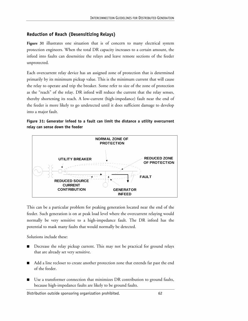
INTERCONNECTION GUIDELINES FOR DISTRIBUTED GENERATION
Distribution outside sponsoring organization prohibited. 62
Reduction of Reach (Desensitizing Relays)
Figure 31 illustrates one situation that is of concern to many electrical system
protection engineers. When the total DR capacity increases to a certain amount, the
infeed into faults can desensitize the relays and leave remote sections of the feeder
unprotected.
Each overcurrent relay device has an assigned zone of protection that is determined
primarily by its minimum pickup value. This is the minimum current that will cause
the relay to operate and trip the breaker. Some refer to size of the zone of protection
as the “reach” of the relay. DR infeed will reduce the current that the relay senses,
thereby shortening its reach. A low-current (high-impedance) fault near the end of
the feeder is more likely to go undetected until it does sufficient damage to develop
into a major fault.
Figure 31: Generator infeed to a fault can limit the distance a utility overcurrent relay can sense down the feeder
This can be a particular problem for peaking generation located near the end of the
feeder. Such generation is on at peak load level where the overcurrent relaying would
normally be very sensitive to a high-impedance fault. The DR infeed has the
potential to mask many faults that would normally be detected.
Solutions include these:
■ Decrease the relay pickup current. This may not be practical for ground relays that are already set very sensitive.
■ Add a line recloser to create another protection zone that extends far past the end of the feeder.
■ Use a transformer connection that minimizes DR contribution to ground faults, because high-impedance faults are likely to be ground faults.
FAULTREDUCED SOURCE
CURRENTCONTRIBUTION GENERATOR
INFEED
UTILITY BREAKER
NORMAL ZONE OFPROTECTION
REDUCED ZONEOF PROTECTION
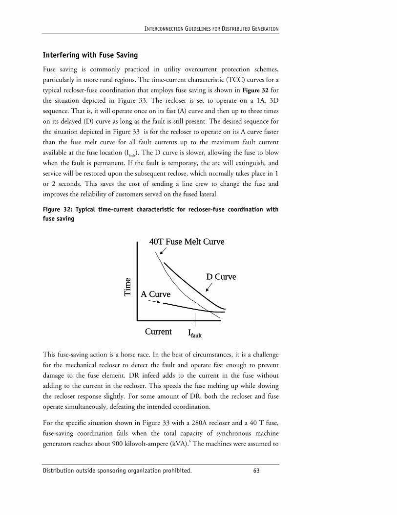
INTERCONNECTION GUIDELINES FOR DISTRIBUTED GENERATION
Distribution outside sponsoring organization prohibited. 63
Interfering with Fuse Saving
Fuse saving is commonly practiced in utility overcurrent protection schemes,
particularly in more rural regions. The time-current characteristic (TCC) curves for a
typical recloser-fuse coordination that employs fuse saving is shown in Figure 32 for
the situation depicted in Figure 33. The recloser is set to operate on a 1A, 3D
sequence. That is, it will operate once on its fast (A) curve and then up to three times
on its delayed (D) curve as long as the fault is still present. The desired sequence for
the situation depicted in Figure 33 is for the recloser to operate on its A curve faster
than the fuse melt curve for all fault currents up to the maximum fault current
available at the fuse location (Ifault). The D curve is slower, allowing the fuse to blow
when the fault is permanent. If the fault is temporary, the arc will extinguish, and
service will be restored upon the subsequent reclose, which normally takes place in 1
or 2 seconds. This saves the cost of sending a line crew to change the fuse and
improves the reliability of customers served on the fused lateral.
Figure 32: Typical time-current characteristic for recloser-fuse coordination with fuse saving
This fuse-saving action is a horse race. In the best of circumstances, it is a challenge
for the mechanical recloser to detect the fault and operate fast enough to prevent
damage to the fuse element. DR infeed adds to the current in the fuse without
adding to the current in the recloser. This speeds the fuse melting up while slowing
the recloser response slightly. For some amount of DR, both the recloser and fuse
operate simultaneously, defeating the intended coordination.
For the specific situation shown in Figure 33 with a 280A recloser and a 40 T fuse,
fuse-saving coordination fails when the total capacity of synchronous machine
generators reaches about 900 kilovolt-ampere (kVA).6 The machines were assumed to
Ifault
D Curve
A Curve
40T Fuse Melt Curve
Tim
e
Current Ifault
D Curve
A Curve
40T Fuse Melt Curve
Tim
e
Current
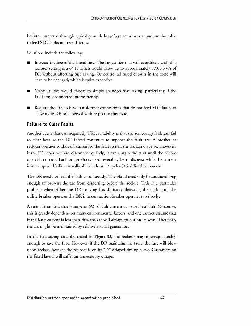
INTERCONNECTION GUIDELINES FOR DISTRIBUTED GENERATION
Distribution outside sponsoring organization prohibited. 64
be interconnected through typical grounded-wye/wye transformers and are thus able
to feed SLG faults on fused laterals.
Solutions include the following:
■ Increase the size of the lateral fuse. The largest size that will coordinate with this recloser setting is a 65T, which would allow up to approximately 1,500 kVA of DR without affecting fuse saving. Of course, all fused cutouts in the zone will have to be changed, which is quite expensive.
■ Many utilities would choose to simply abandon fuse saving, particularly if the DR is only connected intermittently.
■ Require the DR to have transformer connections that do not feed SLG faults to allow more DR to be served with respect to this issue.
Failure to Clear Faults
Another event that can negatively affect reliability is that the temporary fault can fail
to clear because the DR infeed continues to support the fault arc. A breaker or
recloser operates to shut off current to the fault so that the arc can disperse. However,
if the DG does not also disconnect quickly, it can sustain the fault until the reclose
operation occurs. Fault arc products need several cycles to disperse while the current
is interrupted. Utilities usually allow at least 12 cycles (0.2 s) for this to occur.
The DR need not feed the fault continuously. The island need only be sustained long
enough to prevent the arc from dispersing before the reclose. This is a particular
problem when either the DR relaying has difficulty detecting the fault until the
utility breaker opens or the DR interconnection breaker operates too slowly.
A rule of thumb is that 5 amperes (A) of fault current can sustain a fault. Of course,
this is greatly dependent on many environmental factors, and one cannot assume that
if the fault current is less than this, the arc will always go out on its own. Therefore,
the arc might be maintained by relatively small generation.
In the fuse-saving case illustrated in Figure 33, the recloser may interrupt quickly
enough to save the fuse. However, if the DR maintains the fault, the fuse will blow
upon reclose, because the recloser is on its “D” delayed timing curve. Customers on
the fused lateral will suffer an unnecessary outage.
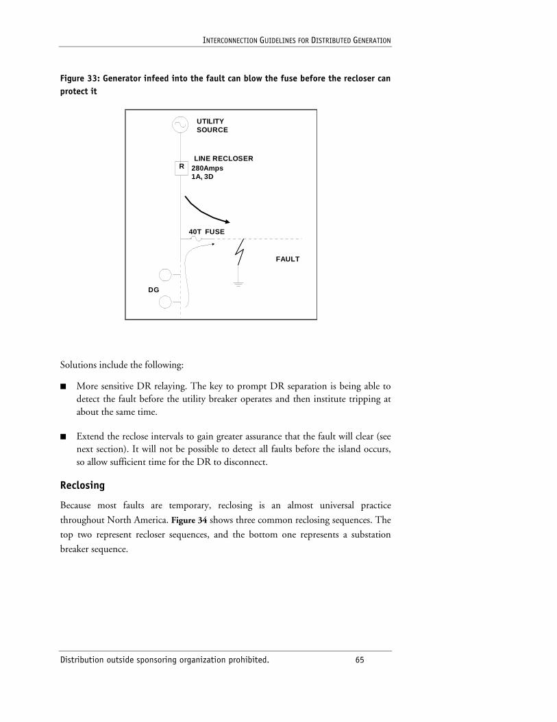
INTERCONNECTION GUIDELINES FOR DISTRIBUTED GENERATION
Distribution outside sponsoring organization prohibited. 65
Figure 33: Generator infeed into the fault can blow the fuse before the recloser can protect it
Solutions include the following:
■ More sensitive DR relaying. The key to prompt DR separation is being able to detect the fault before the utility breaker operates and then institute tripping at about the same time.
■ Extend the reclose intervals to gain greater assurance that the fault will clear (see next section). It will not be possible to detect all faults before the island occurs, so allow sufficient time for the DR to disconnect.
Reclosing
Because most faults are temporary, reclosing is an almost universal practice
throughout North America. Figure 34 shows three common reclosing sequences. The
top two represent recloser sequences, and the bottom one represents a substation
breaker sequence.
R
FAULT
40T FUSE
280Amps1A, 3D
DG
UTILITYSOURCE
LINE RECLOSER
INTERCONNECTION GUIDELINES FOR DISTRIBUTED GENERATION
Distribution outside sponsoring organization prohibited. 66
Figure 34: Some typical reclosing sequences employed by utilities
Because breaker and recloser technologies evolved separately, the philosophies of
operation differ. The intervals between operations tend to be more uniform for
reclosers, although modern controls allow considerable flexibility. The reclose times
for breakers are counted from the first trip operation. The common 0-15-45 reclose
sequence means that the first reclose occurs as fast as possible (also called
“instantaneous reclose”), the second reclose occurs a little less than 15 seconds later,
and the final one occurs approximately 30 seconds after the second.
Regardless of the sequence, the main idea is for temporary faults to clear during the
interval between reclose operations. This is commonly referred to as the “reclose
interval” between “shots.”
DR must disconnect early in the first reclose interval to allow the normal fault-
clearing sequence to proceed successfully. There are two generally bad consequences
if this fails to happen:
■ The fault fails to clear, resulting in at least one more operation of the fault interrupter. This increases the chance of damage to utility facilities and may subject customers to unnecessary outages.
DR must disconnect by this time
DR must disconnect by this time
INTERCONNECTION GUIDELINES FOR DISTRIBUTED GENERATION
Distribution outside sponsoring organization prohibited. 67
■ The DR is still connected when the reclose occurs, resulting in damage to the distributed resource. This is less of a concern with inverter-based distributed resources, which have little inertia. However, it is an important concern for rotating machines, which can suffer winding and shaft damage due to out-of-phase switching forces.
Solutions include the following:
■ Extend the first reclose interval. This is particularly important if the utility is accustomed to using instantaneous reclose. This greatly increases the chances of reclosing with DR still connected. Extending the interval to 1 second (s)or more will help ensure that the DR is off line. A few utilities require 5 s for the first reclose interval on any feeder containing DR. IEEE P1547 recommends a 10-cycle (0.16-s) delay on tripping to avoid nuisance tripping. This takes up a significant portion of an instantaneous reclose interval, which ranges from 0.2 to 0.5 s. Instantaneous reclose and DR are fundamentally incompatible.
■ Employ more-sensitive fault detection. A key to disconnecting the DR soon after the utility breaker operates is to anticipate the operation. This means detecting the fault at nearly the same time as the utility breaker detects it. One difficulty will be that the voltages seen by the DR relaying will frequently not be low enough during the fault. Negative sequence and reverse power (for non-exporting facilities) relaying can increase sensitivity.
5.3 Improving Reliability with DR
One does not have to look far into the DR literature to find statements claiming that
one advantage of distributed generation is improved reliability. As we shall see, the
validity of that claim depends on one’s viewpoint and how one defines reliability.
In this section, we look at some applications where there is an improvement in
reliability. Then in the subsequent section we evaluate applications that degraded
reliability.
Whose Reliability?
One of the first questions we must deal with is to clarify whose reliability is being
improved. This document is intended primarily for a utility audience, but it is not
always clear that the utility will realize a reliability benefit from DR. Most of the gain
in reliability goes to individual customers who have invested in DR that can also
serve as backup generation when the utility system is down.
When a utility looks at reliability, it is generally in terms of the standard reliability
indices that measure the average rates of quantities relevant to the sustained
interruptions of power in the system. For example, one standard measure of the
INTERCONNECTION GUIDELINES FOR DISTRIBUTED GENERATION
Distribution outside sponsoring organization prohibited. 68
performance of utility systems is the System Average Interruption Frequency Index
(SAIFI), often written as
This index is a measure of how often the average customer in the system is
interrupted each year. The value is highly dependent on how one defines “system.”
Typically, utilities will report these values’ average over most, if not all, of their
service territory. A typical target for SAIFI ranges from 0.5 to 1.0. For a large system
with thousands of customers, the reliability improvement achieved for one customer
with backup generation is barely noticeable.
With the advent of better power quality–monitoring equipment and databases, some
utilities are able to scale the indices down to individual feeders or even sections of
feeders. Even from this perspective, the impact of DR on reliability is small. To see a
noticeable improvement in these indices, one would have to be able to restore service
to many customers by forming an independent island served by backup generation.
This is done by some utilities when serving remote areas by a single feed, but it is not
common. Most prefer to build alternate feeds by wire where that is economically
practical. For liability reasons, there is almost universal opposition to employing
customer-owned generation to form such islands.
If we scale this analysis down to a single customer, the perspective changes radically.
Although the average customer may experience only one interruption per year, some
may experience considerably more. Customers in rural areas where there are trees
along the feeders may experience four or more interruptions of three hours each. If
the value of the load justifies backup generation, customers—commercial and
industrial customers in particular—can expect a tremendous improvement in
electricity reliability by installing distributed generation.
Next, we examine three DR applications that can result in reliability benefits to the
utility system as a whole. Then we examine the use of DG for backup purposes by
customers seeking to improve reliability—by, essentially, the formation of single-
customer islands.
Siting for Transmission Support
Support for the transmission grid can be accomplished with DR connected to either
the transmission or the distribution system. It is common for utilities to install
peaking generation in their substations. This is convenient to the utility, because it
SAIFI(No. Customers Interrupted)(No. of Interruptions)
Total No Customers=
.
INTERCONNECTION GUIDELINES FOR DISTRIBUTED GENERATION
Distribution outside sponsoring organization prohibited. 69
has control over the property, and substations also are likely to have connections to
utility energy management systems. This enables the utility to ensure that the
generation will be deployed as necessary to support the system.
Generation installed on the distribution system is likely to be customer controlled.
However, its use may benefit portions of the transmission system. In fact, there is
sometimes a bonus ranging from 5 percent to 20 percent with respect to transmission
relief, depending on where the generation is located on the feeder and how heavily
the feeder is loaded. The generator will reduce the losses and the reactive power
required to serve the load. For example, a 1-megawatt (MW) generator may reduce
the total demand on the transmission grid by 1.1 MW. On some severely
constrained systems, this can have a ripple effect back through the system, allowing
considerably more than 1 MW of additional load to be served.
The amount of capacity relief that DR brings to the transmission system depends on
a number of factors. Location is very important, and not every substation is in a good
position to offer relief. Others are in severely constrained areas where a little load
relief allows the transmission grid to serve several times that amount of load. If the
issue is simply the supply of electricity, and there are no grid constraints, then the
generation may be located on any substation in the service territory. However, DR
located in some areas will have a greater benefit than in other areas.
The value of DR in a particular location is determined by power flow studies. Figure
35 shows the results of determining the value based on loss reduction for a
transmission grid. Each filled circle represents a bus. The numbered buses indicate
the top six locations for 5-MW units for a particular contingency condition. A
different contingency may yield a completely different solution. Also, assuming a
different unit size would shift the distribution of generators slightly. One result of
this analysis that’s of interest to utility engineers is knowing where distributed
generation might be helpful. If this is the limiting contingency, some special effort
can be made to acquire generation on the substations at the buses shown.
The criteria for selecting the “optimal” site also have a great influence on the result.
Although losses are a good metric to use in general, because the results tend to
naturally alleviate congestion, there are other methods. For example, losses may be
weighted by the degree of line overloads. This will result in DR sites that reduce the
flows in the most heavily loaded lines that have a significant amount of losses.
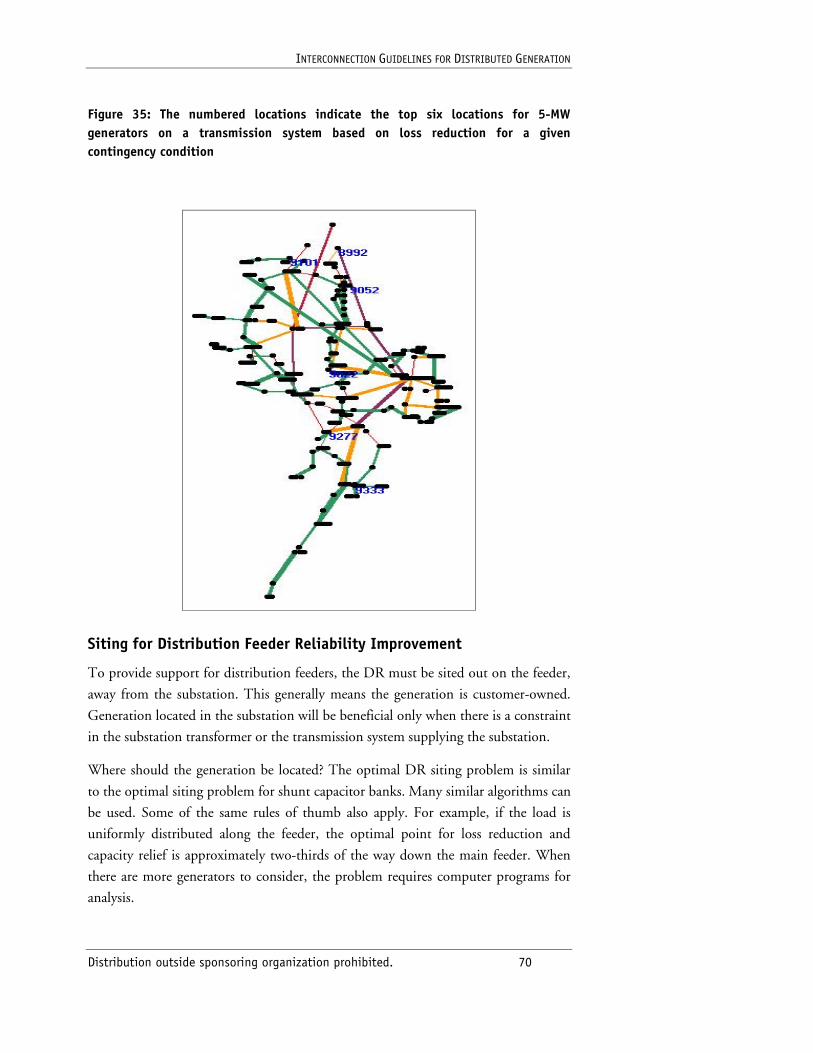
INTERCONNECTION GUIDELINES FOR DISTRIBUTED GENERATION
Distribution outside sponsoring organization prohibited. 70
Figure 35: The numbered locations indicate the top six locations for 5-MW generators on a transmission system based on loss reduction for a given contingency condition
Siting for Distribution Feeder Reliability Improvement
To provide support for distribution feeders, the DR must be sited out on the feeder,
away from the substation. This generally means the generation is customer-owned.
Generation located in the substation will be beneficial only when there is a constraint
in the substation transformer or the transmission system supplying the substation.
Where should the generation be located? The optimal DR siting problem is similar
to the optimal siting problem for shunt capacitor banks. Many similar algorithms can
be used. Some of the same rules of thumb also apply. For example, if the load is
uniformly distributed along the feeder, the optimal point for loss reduction and
capacity relief is approximately two-thirds of the way down the main feeder. When
there are more generators to consider, the problem requires computer programs for
analysis.
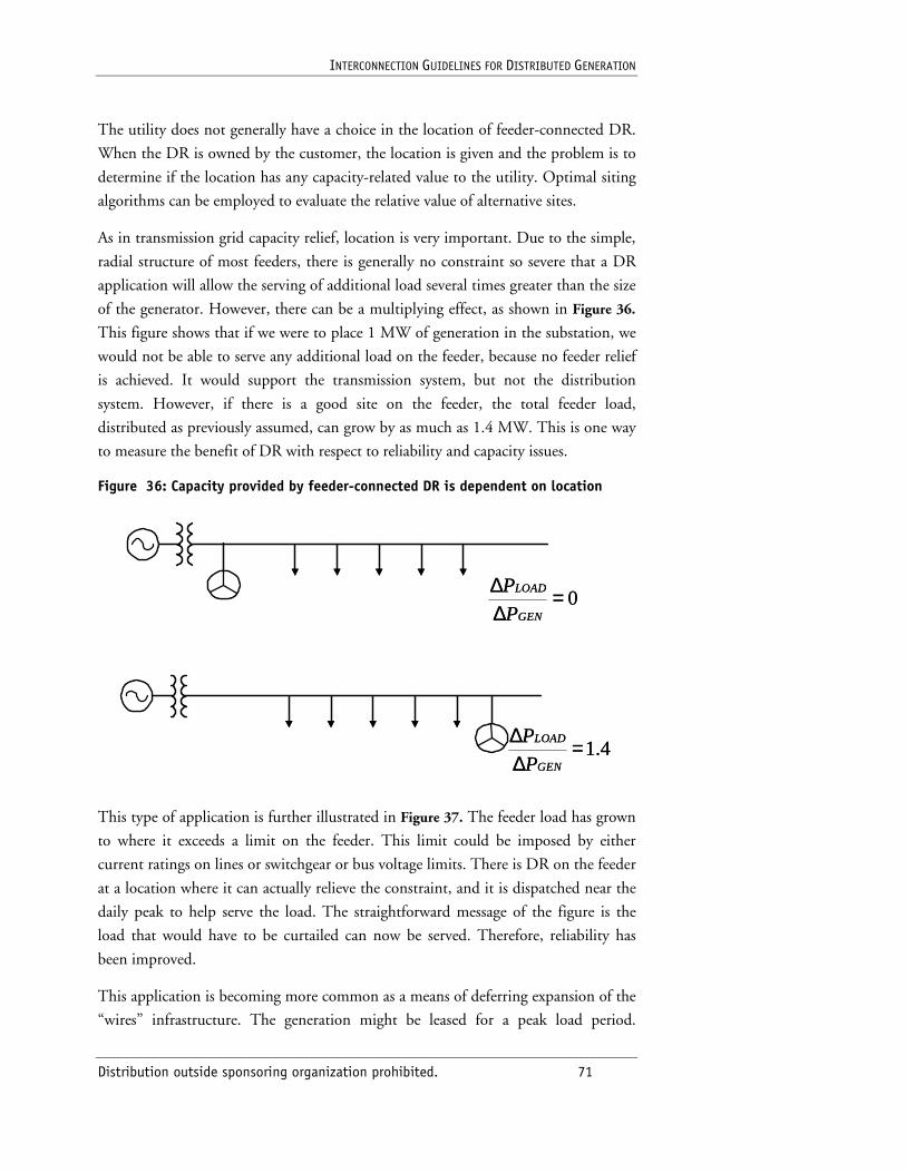
INTERCONNECTION GUIDELINES FOR DISTRIBUTED GENERATION
Distribution outside sponsoring organization prohibited. 71
The utility does not generally have a choice in the location of feeder-connected DR.
When the DR is owned by the customer, the location is given and the problem is to
determine if the location has any capacity-related value to the utility. Optimal siting
algorithms can be employed to evaluate the relative value of alternative sites.
As in transmission grid capacity relief, location is very important. Due to the simple,
radial structure of most feeders, there is generally no constraint so severe that a DR
application will allow the serving of additional load several times greater than the size
of the generator. However, there can be a multiplying effect, as shown in Figure 36.
This figure shows that if we were to place 1 MW of generation in the substation, we
would not be able to serve any additional load on the feeder, because no feeder relief
is achieved. It would support the transmission system, but not the distribution
system. However, if there is a good site on the feeder, the total feeder load,
distributed as previously assumed, can grow by as much as 1.4 MW. This is one way
to measure the benefit of DR with respect to reliability and capacity issues.
Figure 36: Capacity provided by feeder-connected DR is dependent on location
0=∆∆
GEN
LOAD
P
P
4.1=∆∆
GEN
LOAD
P
P
0=∆∆
GEN
LOAD
P
P
4.1=∆∆
GEN
LOAD
P
P
This type of application is further illustrated in Figure 37. The feeder load has grown
to where it exceeds a limit on the feeder. This limit could be imposed by either
current ratings on lines or switchgear or bus voltage limits. There is DR on the feeder
at a location where it can actually relieve the constraint, and it is dispatched near the
daily peak to help serve the load. The straightforward message of the figure is the
load that would have to be curtailed can now be served. Therefore, reliability has
been improved.
This application is becoming more common as a means of deferring expansion of the
“wires” infrastructure. The generation might be leased for a peak load period.
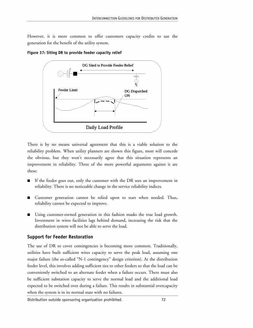
INTERCONNECTION GUIDELINES FOR DISTRIBUTED GENERATION
Distribution outside sponsoring organization prohibited. 72
However, it is more common to offer customers capacity credits to use the
generation for the benefit of the utility system.
Figure 37: Siting DR to provide feeder capacity relief
Daily Load Profile
Feeder Limit DG Dispatched ON
DG Sited to Provide Feeder Relief
Daily Load Profile
Feeder Limit DG Dispatched ON
DG Sited to Provide Feeder Relief
There is by no means universal agreement that this is a viable solution to the
reliability problem. When utility planners are shown this figure, most will concede
the obvious, but they won’t necessarily agree that this situation represents an
improvement in reliability. Three of the more powerful arguments against it are
these:
■ If the feeder goes out, only the customer with the DR sees an improvement in reliability. There is no noticeable change in the service reliability indices.
■ Customer generation cannot be relied upon to start when needed. Thus, reliability cannot be expected to improve.
■ Using customer-owned generation in this fashion masks the true load growth. Investment in wires facilities lags behind demand, increasing the risk that the distribution system will not be able to serve the load.
Support for Feeder Restoration
The use of DR to cover contingencies is becoming more common. Traditionally,
utilities have built sufficient wires capacity to serve the peak load, assuming one
major failure (the so-called “N-1 contingency” design criterion). At the distribution
feeder level, this involves adding sufficient ties to other feeders so that the load can be
conveniently switched to an alternate feeder when a failure occurs. There must also
be sufficient substation capacity to serve the normal load and the additional load
expected to be switched over during a failure. This results in substantial overcapacity
when the system is in its normal state with no failures.
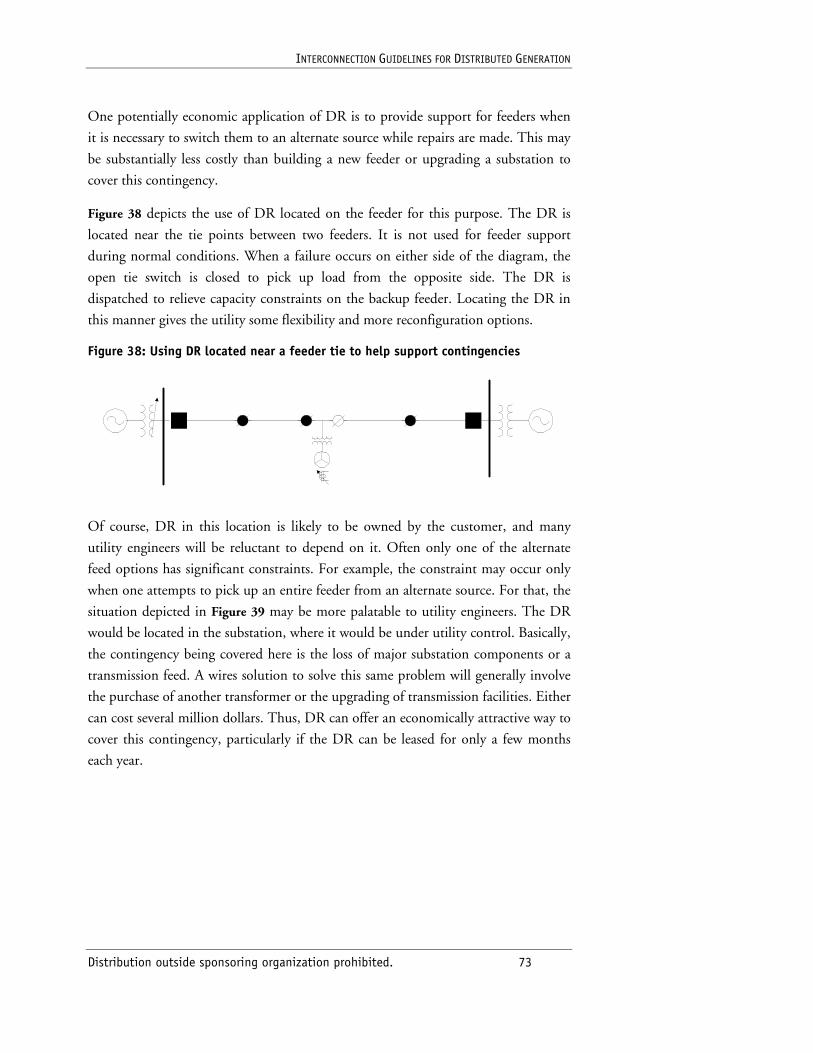
INTERCONNECTION GUIDELINES FOR DISTRIBUTED GENERATION
Distribution outside sponsoring organization prohibited. 73
One potentially economic application of DR is to provide support for feeders when
it is necessary to switch them to an alternate source while repairs are made. This may
be substantially less costly than building a new feeder or upgrading a substation to
cover this contingency.
Figure 38 depicts the use of DR located on the feeder for this purpose. The DR is
located near the tie points between two feeders. It is not used for feeder support
during normal conditions. When a failure occurs on either side of the diagram, the
open tie switch is closed to pick up load from the opposite side. The DR is
dispatched to relieve capacity constraints on the backup feeder. Locating the DR in
this manner gives the utility some flexibility and more reconfiguration options.
Figure 38: Using DR located near a feeder tie to help support contingencies
Of course, DR in this location is likely to be owned by the customer, and many
utility engineers will be reluctant to depend on it. Often only one of the alternate
feed options has significant constraints. For example, the constraint may occur only
when one attempts to pick up an entire feeder from an alternate source. For that, the
situation depicted in Figure 39 may be more palatable to utility engineers. The DR
would be located in the substation, where it would be under utility control. Basically,
the contingency being covered here is the loss of major substation components or a
transmission feed. A wires solution to solve this same problem will generally involve
the purchase of another transformer or the upgrading of transmission facilities. Either
can cost several million dollars. Thus, DR can offer an economically attractive way to
cover this contingency, particularly if the DR can be leased for only a few months
each year.
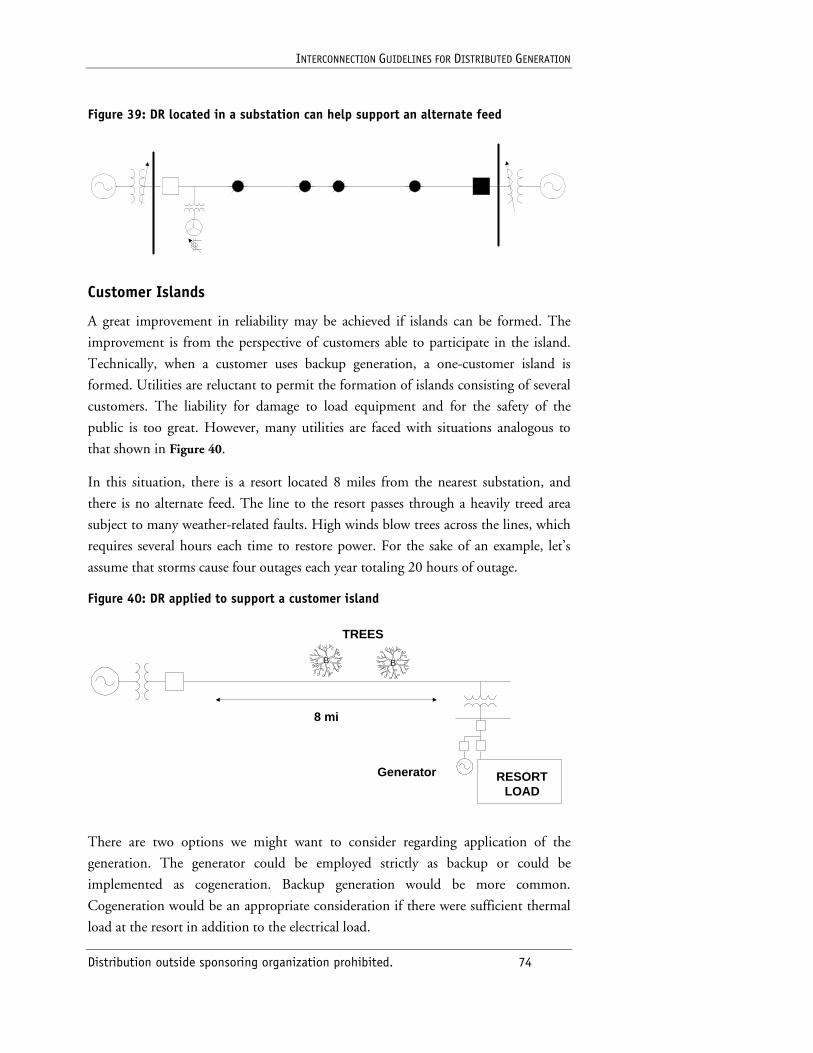
INTERCONNECTION GUIDELINES FOR DISTRIBUTED GENERATION
Distribution outside sponsoring organization prohibited. 74
Figure 39: DR located in a substation can help support an alternate feed
Customer Islands
A great improvement in reliability may be achieved if islands can be formed. The
improvement is from the perspective of customers able to participate in the island.
Technically, when a customer uses backup generation, a one-customer island is
formed. Utilities are reluctant to permit the formation of islands consisting of several
customers. The liability for damage to load equipment and for the safety of the
public is too great. However, many utilities are faced with situations analogous to
that shown in Figure 40.
In this situation, there is a resort located 8 miles from the nearest substation, and
there is no alternate feed. The line to the resort passes through a heavily treed area
subject to many weather-related faults. High winds blow trees across the lines, which
requires several hours each time to restore power. For the sake of an example, let’s
assume that storms cause four outages each year totaling 20 hours of outage.
Figure 40: DR applied to support a customer island
8 mi
RESORTLOAD
B B
Generator
TREES
There are two options we might want to consider regarding application of the
generation. The generator could be employed strictly as backup or could be
implemented as cogeneration. Backup generation would be more common.
Cogeneration would be an appropriate consideration if there were sufficient thermal
load at the resort in addition to the electrical load.
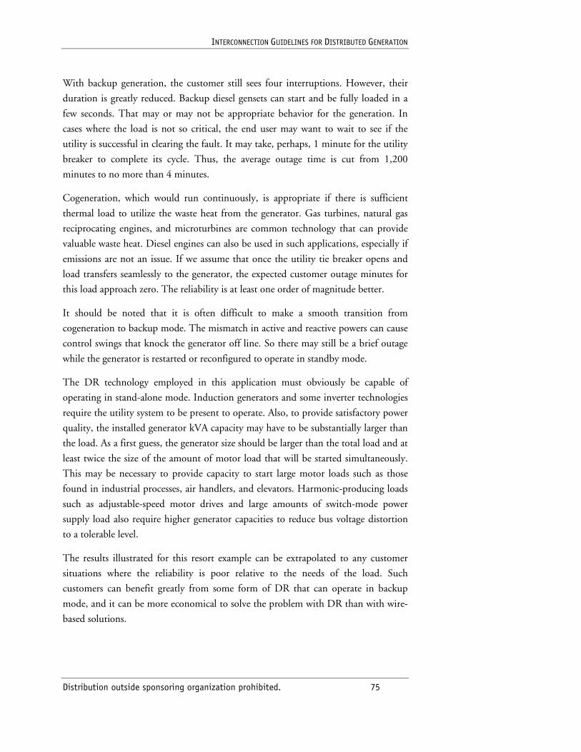
INTERCONNECTION GUIDELINES FOR DISTRIBUTED GENERATION
Distribution outside sponsoring organization prohibited. 75
With backup generation, the customer still sees four interruptions. However, their
duration is greatly reduced. Backup diesel gensets can start and be fully loaded in a
few seconds. That may or may not be appropriate behavior for the generation. In
cases where the load is not so critical, the end user may want to wait to see if the
utility is successful in clearing the fault. It may take, perhaps, 1 minute for the utility
breaker to complete its cycle. Thus, the average outage time is cut from 1,200
minutes to no more than 4 minutes.
Cogeneration, which would run continuously, is appropriate if there is sufficient
thermal load to utilize the waste heat from the generator. Gas turbines, natural gas
reciprocating engines, and microturbines are common technology that can provide
valuable waste heat. Diesel engines can also be used in such applications, especially if
emissions are not an issue. If we assume that once the utility tie breaker opens and
load transfers seamlessly to the generator, the expected customer outage minutes for
this load approach zero. The reliability is at least one order of magnitude better.
It should be noted that it is often difficult to make a smooth transition from
cogeneration to backup mode. The mismatch in active and reactive powers can cause
control swings that knock the generator off line. So there may still be a brief outage
while the generator is restarted or reconfigured to operate in standby mode.
The DR technology employed in this application must obviously be capable of
operating in stand-alone mode. Induction generators and some inverter technologies
require the utility system to be present to operate. Also, to provide satisfactory power
quality, the installed generator kVA capacity may have to be substantially larger than
the load. As a first guess, the generator size should be larger than the total load and at
least twice the size of the amount of motor load that will be started simultaneously.
This may be necessary to provide capacity to start large motor loads such as those
found in industrial processes, air handlers, and elevators. Harmonic-producing loads
such as adjustable-speed motor drives and large amounts of switch-mode power
supply load also require higher generator capacities to reduce bus voltage distortion
to a tolerable level.
The results illustrated for this resort example can be extrapolated to any customer
situations where the reliability is poor relative to the needs of the load. Such
customers can benefit greatly from some form of DR that can operate in backup
mode, and it can be more economical to solve the problem with DR than with wire-
based solutions.
INTERCONNECTION GUIDELINES FOR DISTRIBUTED GENERATION
Distribution outside sponsoring organization prohibited. 76
5.4 Adverse Impacts of DR on Utility Reliability
In this section we explore several situations in which DR is detrimental to the
reliability of the electric power system. The issues raised form the core of the
reasoning behind the interconnection requirements found in the IEEE P1547
document.
Interference with Utility Fault-Clearing Process
The root cause of most interconnection conflicts for distributed resources that are
interconnected with utility distribution systems has to do with the actions that must
be taken to clear primary-side faults. Several examples have been discussed in great
detail in the first part of this section.
When faults fail to clear, some reliability effects are immediate, while others may take
years to surface. In many cases, the failed fault clearing will simply appear to result in
only a second, unnecessary breaker operation. This subjects line equipment to
additional short-circuit stresses. Substation transformers can fail due to through-fault
forces. Not only is this costly to the utility, but customer loads are also frequently
curtailed until a spare transformer can be moved in.
In other cases, failure to clear a fault means a fuse blows that otherwise would have
been saved. Customers on the affected lateral will suffer an outage typically ranging
in duration from 30 minutes to 3 hours.
Some utilities make only one attempt to clear faults. Therefore, failure to clear a
temporary fault results in a breaker lockout and an outage for all the load on the
feeder.
Extending reclose intervals also has a reliability impact. Utilities that use
instantaneous reclosing have done so because a significant number of customers
benefit by being able to ride through the very short interruption. Increasing the
interval time will cause many to shut down. For some processes, a momentary
interruption of 1 second is the same as a 4-hour sustained interruption for other
customers.
Masking of True Load Growth
This issue is one of the main reasons why many distribution planners will not give
credit for DR in capacity planning studies. If interconnected DR usage becomes
prevalent, the loading signals normally apparent in the substation are masked. Unless
special effort is made to keep track of all the DR installations, the planner is not
certain what the true capacity margin is.
INTERCONNECTION GUIDELINES FOR DISTRIBUTED GENERATION
Distribution outside sponsoring organization prohibited. 77
There are at least two conditions in which this presents an operational issue that can
result in reduced system reliability:
■ All DR is required to disconnect to allow for clearing of faults. If the base capacity in the circuit isn’t there, the reclose operation will result in low voltages and overloaded feeders when a fault occurs at peak loading. Load will have to be curtailed unless many of the DR sites also disconnect the load with the generation.
■ The DR is not available at peak loading. This can happen for a variety of reasons, including equipment failure. However, there is also concern that the DR owner will be out of business or be otherwise financially unable to run the DR.
Therefore, utility planners often insist on building sufficient capacity to serve all the
load and will consider DR only as a temporary bridge to cover capacity shortages
while new base wires capacity is being built. As time passes and nothing is done to
improve base capacity, the view of the planner is that the loading eventually reaches a
point where the reliability is compromised.
Insufficient Amount of DR
Not only can there be so much DR that the load growth is masked, but having too
little can also impact reliability. It almost always takes a certain minimum amount of
DR before there is sufficient capacity to allow additional load to be served, either in
normal or contingency configurations.
Utilities are often faced with distribution capacity shortfalls of a few megawatts. To
solve this problem, they may develop a program to encourage the use of small,
energy-efficient DR by customers. However, it may take years to get enough capacity
in place to create a positive effect on reliability. This is the main reason why many
utilities choose to lease gensets in sufficient quantity rather than relying on customer-
side generation.
This issue highlights one of the key conflicts between utility planning and the use of
DR to support the system. Many of the advantages of DR come through the
application of energy-efficient systems on the customer side. In some cases, these
units may be best applied in sizes of a few kilowatts to a few hundred kilowatts,
whereas it generally requires a few megawatts of DR to defer distribution expansion
plans. Utility planners address their most pressing constraints first, which typically
require investment within one to three years. This is too short a time frame to set up
a program to get customers to install DR capacity in sufficient quantity because of
the high initial investment hurdle. DR is not like demand-side managment programs
that replace relatively low-cost items such as light bulbs, refrigerators, and air
INTERCONNECTION GUIDELINES FOR DISTRIBUTED GENERATION
Distribution outside sponsoring organization prohibited. 78
conditioners. The only options left at this point are either to build new wires capacity
or lease larger-sized gensets. It would be better if smaller DR were targeted to
distribution planning areas that are growing but are several years from reaching a
constraint. This could slow growth sufficiently to eventually allow a significant
deferral.
When the system has evolved to the point where there are many sites of smaller-sized
DR owned by end users, how much capacity credit should be given for planning?
This is a question that can only be answered with time and experience. Assuming the
DR technologies have firm capacities and are not renewables without storage, there
appears to be gathering consensus for discounting the capacity by 30 to 50 percent.
This accounts for units that do not start when called upon for any reason. The units
could be down for maintenance or be prohibited from running because of emissions
limits or workplace rules.
Renewables would be discounted much more, depending on how well the output
coincides with the loading. In certain residential areas, solar photovoltaic (PV) array
output coincides well with the loading peak, and the discounting will be small.
However, in other areas, PV output will miss the 7:00 p.m. dinner-time peak and
must be discounted substantially. There is not a great amount of wind generation
connected to distribution systems, but the output of the existing generation is so
unpredictable that only 5 to 15 percent capacity credit can be given.
Inadvertent Islanding
Perhaps the greatest fear of the utility protection engineer is that DR will fail to
detect the fact that the utility breaker has opened and will continue to energize a
portion of the feeder. Therefore, much attention has been paid to detecting islands or
forcing islands to go unstable so they can be detected (IEEE Standard 929). The
reliability concern is that other customers will be subjected to such poor quality
voltage that equipment damage will be sustained. There is also the safety concern of a
generator accidentally energizing a line that was expected to be dead.
Relaying is one way to address the issue. Another is having requirements for the
operating mode while the DR is interconnected that significantly reduce the chances
that the generation will match the load when an inadvertent island forms:
■ Inverters operating in parallel are less likely to form an island if they are in current-source mode. This requires another source to provide a voltage for the current-source inverter to follow. Of course, this source could be provided by another synchronous generator that remains on the island.
INTERCONNECTION GUIDELINES FOR DISTRIBUTED GENERATION
Distribution outside sponsoring organization prohibited. 79
■ All DR should operate in constant power factor or constant reactive power mode. For many devices, this will be unity power factor, producing watts only. Automatic voltage control (AVC) should be avoided while DR is interconnected unless the generator is directly connected to a control center to receive dispatching signals. Without the ability to regulate voltage, the load-generator match would have to be almost perfect to escape detection by the relaying schemes described in this document.
5.5 Harmonics from DR
Modern Inverter Harmonic Characteristics
All DG technologies that generate either DC or non-power-frequency AC must use
an electronic power inverter to interface with the electric power system. The use of
inverters has in the past resulted in greater harmonic distortion than one might get
from alternators. There are many who still associate DR with bad experiences with
harmonics from electronic power converters. If thyristor-based, line-commutated
inverters were still the norm, this would continue to be a large problem. Fortunately,
inverter manufacturers have adopted switching inverter technologies for the most
part, which has eliminated the bulk of the harmonics problems from inverters.
The early thyristor-based, line-commutated inverters quickly developed a reputation
for being undesirable on the power system. These inverters produced harmonic
currents in similar proportion to loads. Besides contributing to the distortion on the
feeders, one fear was that this type of DG would produce a significant amount of
power at the harmonic frequencies. Such power does little more than contribute to
losses in lines and transformers.
To achieve better control and to avoid harmonics problems, inverter technology has
changed to switched, pulse-width modulated (PWM) technologies, resulting in a
more friendly interface to the electric power system.
Figure 41 shows the basic components of a utility interactive inverter that meets the
requirements of IEEE Standard 929-2000.7 Direct current is supplied on the left
side of the diagram either from a conversion technology that produces DC directly or
from the rectification of AC generator output. Variations of this type of inverter are
commonly employed on fuel cells, microturbines, photovoltaic solar, and some wind
turbines.
The DC voltage is switched at a very high rate with an insulated gate bipolar
transistor (IGBT) switch to create a sinusoidal voltage or current of power frequency.
The switching frequency is typically on the order of 50 to 100 times the power
frequency. The filter on the output attenuates these high-frequency components to
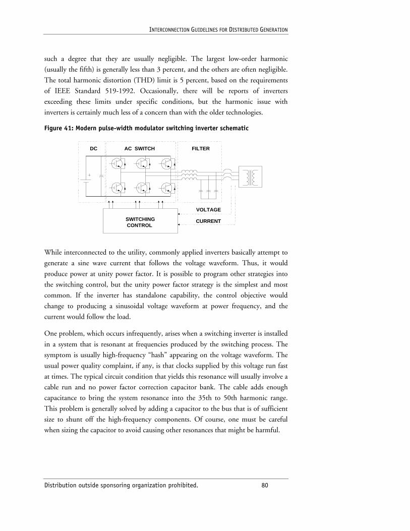
INTERCONNECTION GUIDELINES FOR DISTRIBUTED GENERATION
Distribution outside sponsoring organization prohibited. 80
such a degree that they are usually negligible. The largest low-order harmonic
(usually the fifth) is generally less than 3 percent, and the others are often negligible.
The total harmonic distortion (THD) limit is 5 percent, based on the requirements
of IEEE Standard 519-1992. Occasionally, there will be reports of inverters
exceeding these limits under specific conditions, but the harmonic issue with
inverters is certainly much less of a concern than with the older technologies.
Figure 41: Modern pulse-width modulator switching inverter schematic
SWITCHINGCONTROL
VOLTAGE
CURRENT
FILTERAC SWITCHDC
While interconnected to the utility, commonly applied inverters basically attempt to
generate a sine wave current that follows the voltage waveform. Thus, it would
produce power at unity power factor. It is possible to program other strategies into
the switching control, but the unity power factor strategy is the simplest and most
common. If the inverter has standalone capability, the control objective would
change to producing a sinusoidal voltage waveform at power frequency, and the
current would follow the load.
One problem, which occurs infrequently, arises when a switching inverter is installed
in a system that is resonant at frequencies produced by the switching process. The
symptom is usually high-frequency “hash” appearing on the voltage waveform. The
usual power quality complaint, if any, is that clocks supplied by this voltage run fast
at times. The typical circuit condition that yields this resonance will usually involve a
cable run and no power factor correction capacitor bank. The cable adds enough
capacitance to bring the system resonance into the 35th to 50th harmonic range.
This problem is generally solved by adding a capacitor to the bus that is of sufficient
size to shunt off the high-frequency components. Of course, one must be careful
when sizing the capacitor to avoid causing other resonances that might be harmful.
INTERCONNECTION GUIDELINES FOR DISTRIBUTED GENERATION
Distribution outside sponsoring organization prohibited. 81
Machine Harmonics, Winding Pitch, and the “Harmonic Surprise”
Harmonics from rotating machines are not always negligible, particularly, in grid-
parallel operation. The utility power system acts as a short circuit to zero-sequence
triplen harmonics in the voltage, which can result in surprisingly high currents. For
service transformers connected grounded-wye/wye or delta/wye, only synchronous
machines with two-thirds pitch can be paralleled without special provisions to limit
neutral current. For service transformer connections with a delta-connected winding
on the DG side, nearly any type of three-phase alternator can be paralleled without
this harmonic problem. Refer to the “Harmonic Surprise” section in Section 6 for
additional details.
INTERCONNECTION GUIDELINES FOR DISTRIBUTED GENERATION
Distribution outside sponsoring organization prohibited. 82
6. Application Problems
This section presents a series of mini case studies through which common issues and
problems related to distributed resources (DR) on the distribution system are
illustrated with quantitative examples. The goal is to illustrate problem analysis and
resolution that uses the information and approaches described in previous chapters.
6.1 Voltage Change upon Interconnection or Reclose After a Fault
One of the major limitations on the amount of DR than can be accommodated on a
distribution system without costly changes is how much the system voltage changes
for DR interconnection or disconnection. This is often the principal limitation when
the DR is located a considerable distance from the substation.
There are two conditions of concern: when DR is connected and ramped up to full
power and when DR is forced off to clear faults on the utility system.
The former condition may only be significant when there is a single, large DR
installation. When there are widely distributed DR locations, each making its own
decision about when to connect, the interconnection voltage swing might occur
slowly. This will allow standard utility voltage regulation equipment to keep up with
the voltage change.
Regarding the latter condition, it is a universal requirement for DR to disconnect for
faults on the utility system and remain disconnected for up to 5 minutes (per IEEE
1547). Thus, all the DR will be suddenly removed from the feeder. The voltage
change that occurs when the utility breaker recloses without the DR is often a good
measure of the feeder’s degree of dependence on DR for capacity. If the change is too
great, however that is defined, then changes will have to be made to the system.
One approach to studying this issue is to compute the voltages immediately before
and after the connection to DR is energized. Figure 42 shows the results of one such
study on a 25-kilovolt (kV)–class feeder. This represents the result of thousands of
cases in which the DR was randomly placed along the feeder in random sizes and for
random loadings. The voltage rise when the DR was interconnected was plotted for
each case, and contours of constant voltage change were developed as shown. The
dark heavy lines are a linear approximation to three of the contours: 1.0, 1.05, and
1.10 per unit (pu) voltage. That is, voltage rises of 0, 5 percent, and 10 percent,
respectively.
The contours are plotted as constant voltage for distance from the substation and
excess generation over load. Excess generation is defined as the total DR power
minus the total load power. Though a similar plot could be made using generation
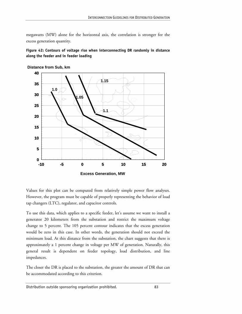
INTERCONNECTION GUIDELINES FOR DISTRIBUTED GENERATION
Distribution outside sponsoring organization prohibited. 83
megawatts (MW) alone for the horizontal axis, the correlation is stronger for the
excess generation quantity.
Figure 42: Contours of voltage rise when interconnecting DR randomly in distance along the feeder and in feeder loading
-10 -5 0 5 10 15 200
5
10
15
20
25
30
35
40
1.0
1.05
1.1
1.15
Distance from Sub, km
Excess Generation, MW
-10 -5 0 5 10 15 200
5
10
15
20
25
30
35
40
1.0
1.05
1.1
1.15
Distance from Sub, km
Excess Generation, MW
Values for this plot can be computed from relatively simple power flow analyses.
However, the program must be capable of properly representing the behavior of load
tap changers (LTC), regulator, and capacitor controls.
To use this data, which applies to a specific feeder, let’s assume we want to install a
generator 20 kilometers from the substation and restrict the maximum voltage
change to 5 percent. The 105 percent contour indicates that the excess generation
would be zero in this case. In other words, the generation should not exceed the
minimum load. At this distance from the substation, the chart suggests that there is
approximately a 1 percent change in voltage per MW of generation. Naturally, this
general result is dependent on feeder topology, load distribution, and line
impedances.
The closer the DR is placed to the substation, the greater the amount of DR that can
be accommodated according to this criterion.
INTERCONNECTION GUIDELINES FOR DISTRIBUTED GENERATION
Distribution outside sponsoring organization prohibited. 84
Symptoms
The symptoms or DR impacts on feeder voltage stability are large voltage changes
that may coincide with other major events such as faults. If there is too much DR on
the feeder with respect to the constraints of excess generation and distance of that
generation from the substation, the voltage will be noticeably low immediately
following a utility breaker operation to clear a fault. This may gradually correct itself
over the next minute or so, depending on the settings on the voltage regulation
equipment.
A rise can also occur if large amounts of DR are energized and ramped up to power
quickly. This might be a large genset used for peaking or a large cogeneration facility
coming on line. It can also happen for numerous small distributed resources after
they are forced off for fault clearing. If they follow the P1547 document, they will
reconnect after a time delay of 5 minutes or some other time specified by the utility.
Solutions
One solution is to require the customer with DR to remove the load as well as the
DR when the DR is forced off. Another is to restore the feeder in stages. Both
solutions may result in poorer reliability for some customers.
The voltage change will be greater when the DR technology produces or consumes
more reactive power. Therefore, another solution is to require the DR to operate near
unity power factor. A voltage change will still occur, but it will be less severe. Unity
power factor is normal for many inverter-connected DR technologies. The reactive
power for induction machines cannot generally be controlled, and external capacitors
must be used to compensate for reactive power consumption. This solution is
acceptable as long as harmonic resonances are avoided and capacitor switching
transients are tolerable.
Another strategy is to stagger the reconnect delay when there are numerous DR
devices so that they don’t all come back on at the same time after fault clearing.
6.2 Harmonic Surprise with Rotating Machines
A commonly held misconception is that standby generation can simply be intertied
parallel with the utility to export power from the generator onto the grid.
Unfortunately, many machines do not have the proper design to accomplish this.
They produce too much third harmonic voltage as a result of their designed winding
pitch. Machines that do not have a two-third pitch winding may generate 5 percent
third harmonic voltage, or more.
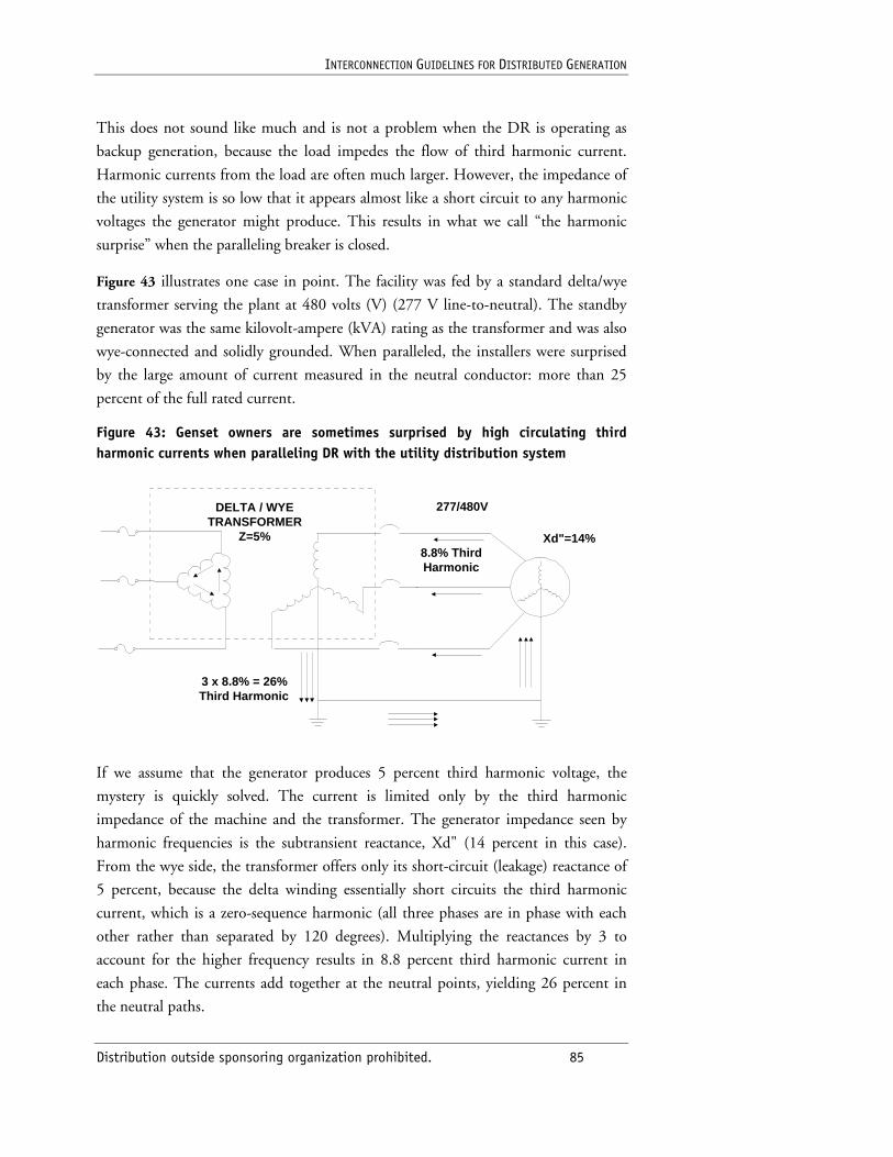
INTERCONNECTION GUIDELINES FOR DISTRIBUTED GENERATION
Distribution outside sponsoring organization prohibited. 85
This does not sound like much and is not a problem when the DR is operating as
backup generation, because the load impedes the flow of third harmonic current.
Harmonic currents from the load are often much larger. However, the impedance of
the utility system is so low that it appears almost like a short circuit to any harmonic
voltages the generator might produce. This results in what we call “the harmonic
surprise” when the paralleling breaker is closed.
Figure 43 illustrates one case in point. The facility was fed by a standard delta/wye
transformer serving the plant at 480 volts (V) (277 V line-to-neutral). The standby
generator was the same kilovolt-ampere (kVA) rating as the transformer and was also
wye-connected and solidly grounded. When paralleled, the installers were surprised
by the large amount of current measured in the neutral conductor: more than 25
percent of the full rated current.
Figure 43: Genset owners are sometimes surprised by high circulating third harmonic currents when paralleling DR with the utility distribution system
If we assume that the generator produces 5 percent third harmonic voltage, the
mystery is quickly solved. The current is limited only by the third harmonic
impedance of the machine and the transformer. The generator impedance seen by
harmonic frequencies is the subtransient reactance, Xd" (14 percent in this case).
From the wye side, the transformer offers only its short-circuit (leakage) reactance of
5 percent, because the delta winding essentially short circuits the third harmonic
current, which is a zero-sequence harmonic (all three phases are in phase with each
other rather than separated by 120 degrees). Multiplying the reactances by 3 to
account for the higher frequency results in 8.8 percent third harmonic current in
each phase. The currents add together at the neutral points, yielding 26 percent in
the neutral paths.
DELTA / WYETRANSFORMER
Z=5%
277/480V
Xd"=14%8.8% ThirdHarmonic
3 x 8.8% = 26%Third Harmonic
INTERCONNECTION GUIDELINES FOR DISTRIBUTED GENERATION
Distribution outside sponsoring organization prohibited. 86
This current simply circulates, causing losses and phase voltage imbalance, which
limits the output of the generator and may interfere with its control. It could also
place excessive duty on neutral conductors, depending on their size.
Symptoms
■ The generator trips out on ground overcurrent or by thermal protection. It is not possible to produce full power from the generator.
■ High neutral currents and unbalanced phase voltages are measured. A power quality monitor would indicate high third harmonic currents and voltages.
■ An infrared scan shows heating at neutral conductor junctions.
Solutions
■ Vendors of engine gensets will generally insist on a two-thirds pitch machine for applications where a backup generator may be connected grid-parallel at some time. If it is not possible to change the machine, a reactor may be inserted in the neutral of the generator to limit the current while the DR is operating in parallel with the grid. When operating in stand-alone backup mode, the reactor may be shorted out with a bypass switch.
■ A different transformer with a delta-connected secondary will prevent the flow of third harmonics. Likewise, a delta-connected alternator will cancel out the third harmonic.
6.3 Desensitizing Utility Relays
Overcurrent relays on the utility system are set to detect a range of fault currents.
The minimum pickup value is selected so that the relay can sense specified high-
resistance faults at a certain location on the feeder. This defines the zone of
protection. This zone should overlap the next series overcurrent device downstream.
If it is the last device, the zone must extend comfortably past the end of the feeder.
Relay settings are established assuming current contributions from only one source.
Some computer programs for computing short circuits consider load effects, while
others ignore it. Normally, it is a minor issue, but when there is considerable
impedance in the circuit and the fault, small changes can make the difference
between detecting a fault and not.
This example describes an analysis to determine the potential impact of DR in the
rural part of a feeder (Figure 44). The feeder is lengthy and consists of an urban
section and a rural section. A Cooper Power Systems VWE line recloser is installed
near the urban/rural boundary. The recloser pickup current was 280 amperes (A),
and its operating sequence was 1A3D.
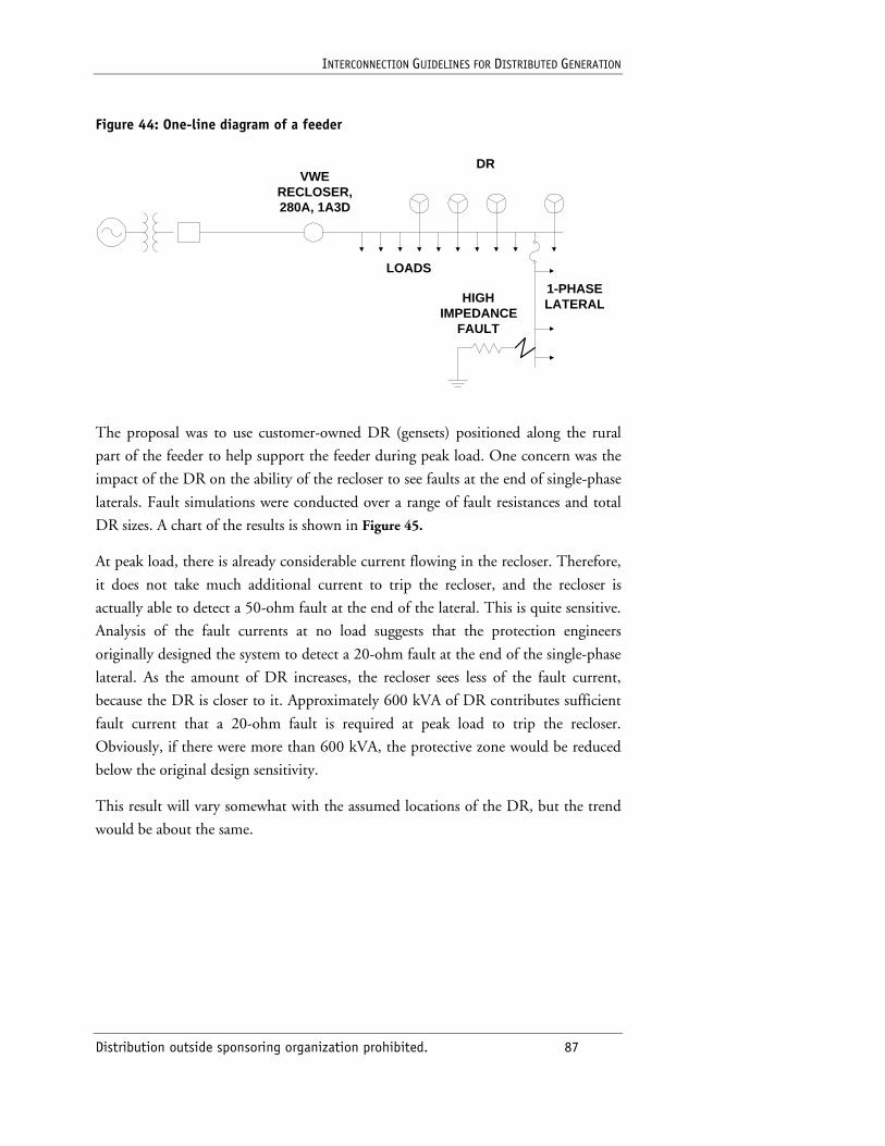
INTERCONNECTION GUIDELINES FOR DISTRIBUTED GENERATION
Distribution outside sponsoring organization prohibited. 87
Figure 44: One-line diagram of a feeder
The proposal was to use customer-owned DR (gensets) positioned along the rural
part of the feeder to help support the feeder during peak load. One concern was the
impact of the DR on the ability of the recloser to see faults at the end of single-phase
laterals. Fault simulations were conducted over a range of fault resistances and total
DR sizes. A chart of the results is shown in Figure 45.
At peak load, there is already considerable current flowing in the recloser. Therefore,
it does not take much additional current to trip the recloser, and the recloser is
actually able to detect a 50-ohm fault at the end of the lateral. This is quite sensitive.
Analysis of the fault currents at no load suggests that the protection engineers
originally designed the system to detect a 20-ohm fault at the end of the single-phase
lateral. As the amount of DR increases, the recloser sees less of the fault current,
because the DR is closer to it. Approximately 600 kVA of DR contributes sufficient
fault current that a 20-ohm fault is required at peak load to trip the recloser.
Obviously, if there were more than 600 kVA, the protective zone would be reduced
below the original design sensitivity.
This result will vary somewhat with the assumed locations of the DR, but the trend
would be about the same.
VWERECLOSER,280A, 1A3D
HIGHIMPEDANCE
FAULT
1-PHASELATERAL
DR
LOADS
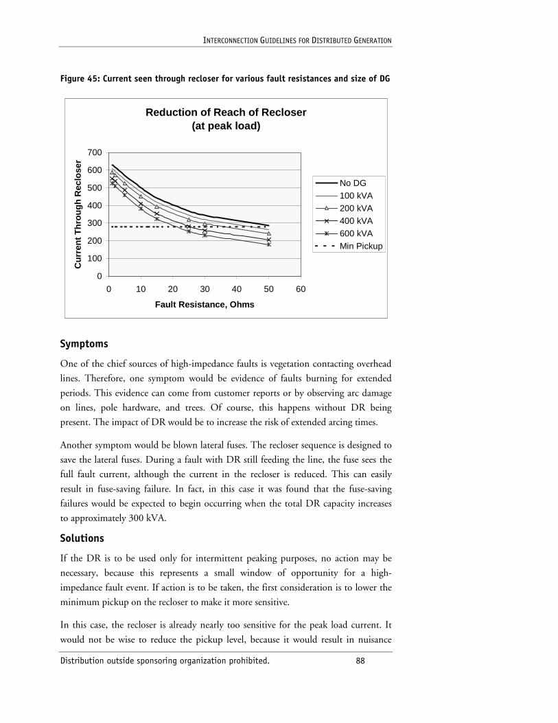
INTERCONNECTION GUIDELINES FOR DISTRIBUTED GENERATION
Distribution outside sponsoring organization prohibited. 88
Figure 45: Current seen through recloser for various fault resistances and size of DG
Reduction of Reach of Recloser(at peak load)
0
100
200
300
400
500
600
700
0 10 20 30 40 50 60
Fault Resistance, Ohms
Cu
rren
t T
hro
ug
h R
eclo
ser
No DG100 kVA200 kVA400 kVA600 kVAMin Pickup
Symptoms
One of the chief sources of high-impedance faults is vegetation contacting overhead
lines. Therefore, one symptom would be evidence of faults burning for extended
periods. This evidence can come from customer reports or by observing arc damage
on lines, pole hardware, and trees. Of course, this happens without DR being
present. The impact of DR would be to increase the risk of extended arcing times.
Another symptom would be blown lateral fuses. The recloser sequence is designed to
save the lateral fuses. During a fault with DR still feeding the line, the fuse sees the
full fault current, although the current in the recloser is reduced. This can easily
result in fuse-saving failure. In fact, in this case it was found that the fuse-saving
failures would be expected to begin occurring when the total DR capacity increases
to approximately 300 kVA.
Solutions
If the DR is to be used only for intermittent peaking purposes, no action may be
necessary, because this represents a small window of opportunity for a high-
impedance fault event. If action is to be taken, the first consideration is to lower the
minimum pickup on the recloser to make it more sensitive.
In this case, the recloser is already nearly too sensitive for the peak load current. It
would not be wise to reduce the pickup level, because it would result in nuisance
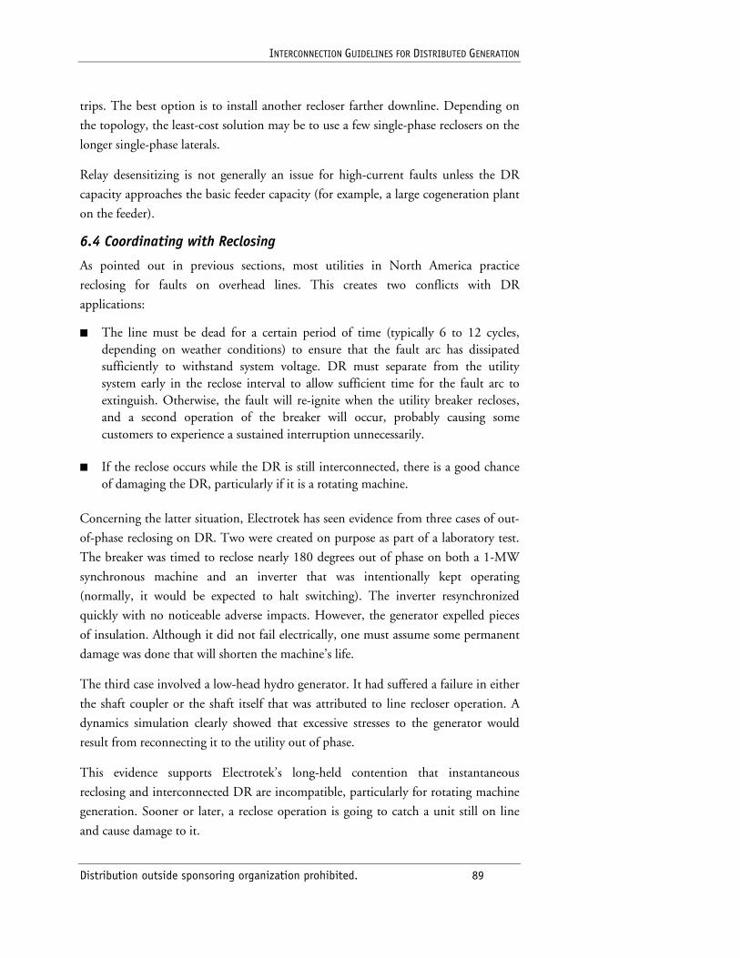
INTERCONNECTION GUIDELINES FOR DISTRIBUTED GENERATION
Distribution outside sponsoring organization prohibited. 89
trips. The best option is to install another recloser farther downline. Depending on
the topology, the least-cost solution may be to use a few single-phase reclosers on the
longer single-phase laterals.
Relay desensitizing is not generally an issue for high-current faults unless the DR
capacity approaches the basic feeder capacity (for example, a large cogeneration plant
on the feeder).
6.4 Coordinating with Reclosing
As pointed out in previous sections, most utilities in North America practice
reclosing for faults on overhead lines. This creates two conflicts with DR
applications:
■ The line must be dead for a certain period of time (typically 6 to 12 cycles, depending on weather conditions) to ensure that the fault arc has dissipated sufficiently to withstand system voltage. DR must separate from the utility system early in the reclose interval to allow sufficient time for the fault arc to extinguish. Otherwise, the fault will re-ignite when the utility breaker recloses, and a second operation of the breaker will occur, probably causing some customers to experience a sustained interruption unnecessarily.
■ If the reclose occurs while the DR is still interconnected, there is a good chance of damaging the DR, particularly if it is a rotating machine.
Concerning the latter situation, Electrotek has seen evidence from three cases of out-
of-phase reclosing on DR. Two were created on purpose as part of a laboratory test.
The breaker was timed to reclose nearly 180 degrees out of phase on both a 1-MW
synchronous machine and an inverter that was intentionally kept operating
(normally, it would be expected to halt switching). The inverter resynchronized
quickly with no noticeable adverse impacts. However, the generator expelled pieces
of insulation. Although it did not fail electrically, one must assume some permanent
damage was done that will shorten the machine’s life.
The third case involved a low-head hydro generator. It had suffered a failure in either
the shaft coupler or the shaft itself that was attributed to line recloser operation. A
dynamics simulation clearly showed that excessive stresses to the generator would
result from reconnecting it to the utility out of phase.
This evidence supports Electrotek’s long-held contention that instantaneous
reclosing and interconnected DR are incompatible, particularly for rotating machine
generation. Sooner or later, a reclose operation is going to catch a unit still on line
and cause damage to it.
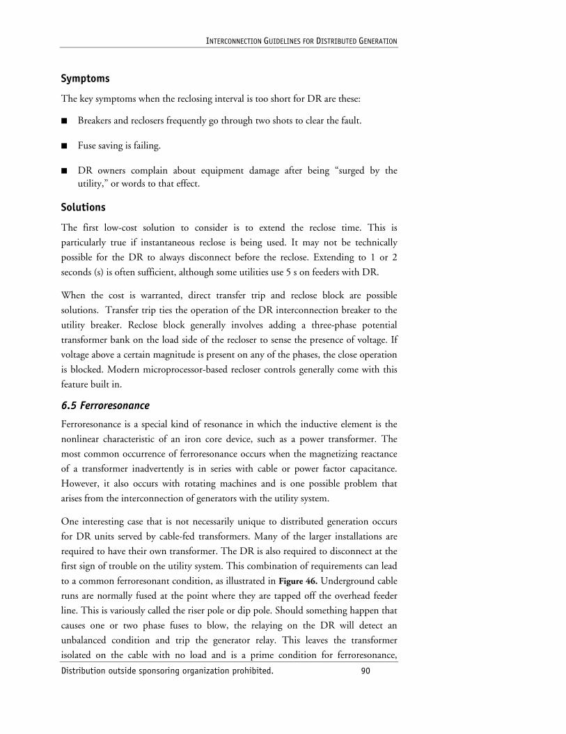
INTERCONNECTION GUIDELINES FOR DISTRIBUTED GENERATION
Distribution outside sponsoring organization prohibited. 90
Symptoms
The key symptoms when the reclosing interval is too short for DR are these:
■ Breakers and reclosers frequently go through two shots to clear the fault.
■ Fuse saving is failing.
■ DR owners complain about equipment damage after being “surged by the utility,” or words to that effect.
Solutions
The first low-cost solution to consider is to extend the reclose time. This is
particularly true if instantaneous reclose is being used. It may not be technically
possible for the DR to always disconnect before the reclose. Extending to 1 or 2
seconds (s) is often sufficient, although some utilities use 5 s on feeders with DR.
When the cost is warranted, direct transfer trip and reclose block are possible
solutions. Transfer trip ties the operation of the DR interconnection breaker to the
utility breaker. Reclose block generally involves adding a three-phase potential
transformer bank on the load side of the recloser to sense the presence of voltage. If
voltage above a certain magnitude is present on any of the phases, the close operation
is blocked. Modern microprocessor-based recloser controls generally come with this
feature built in.
6.5 Ferroresonance
Ferroresonance is a special kind of resonance in which the inductive element is the
nonlinear characteristic of an iron core device, such as a power transformer. The
most common occurrence of ferroresonance occurs when the magnetizing reactance
of a transformer inadvertently is in series with cable or power factor capacitance.
However, it also occurs with rotating machines and is one possible problem that
arises from the interconnection of generators with the utility system.
One interesting case that is not necessarily unique to distributed generation occurs
for DR units served by cable-fed transformers. Many of the larger installations are
required to have their own transformer. The DR is also required to disconnect at the
first sign of trouble on the utility system. This combination of requirements can lead
to a common ferroresonant condition, as illustrated in Figure 46. Underground cable
runs are normally fused at the point where they are tapped off the overhead feeder
line. This is variously called the riser pole or dip pole. Should something happen that
causes one or two phase fuses to blow, the relaying on the DR will detect an
unbalanced condition and trip the generator relay. This leaves the transformer
isolated on the cable with no load and is a prime condition for ferroresonance,
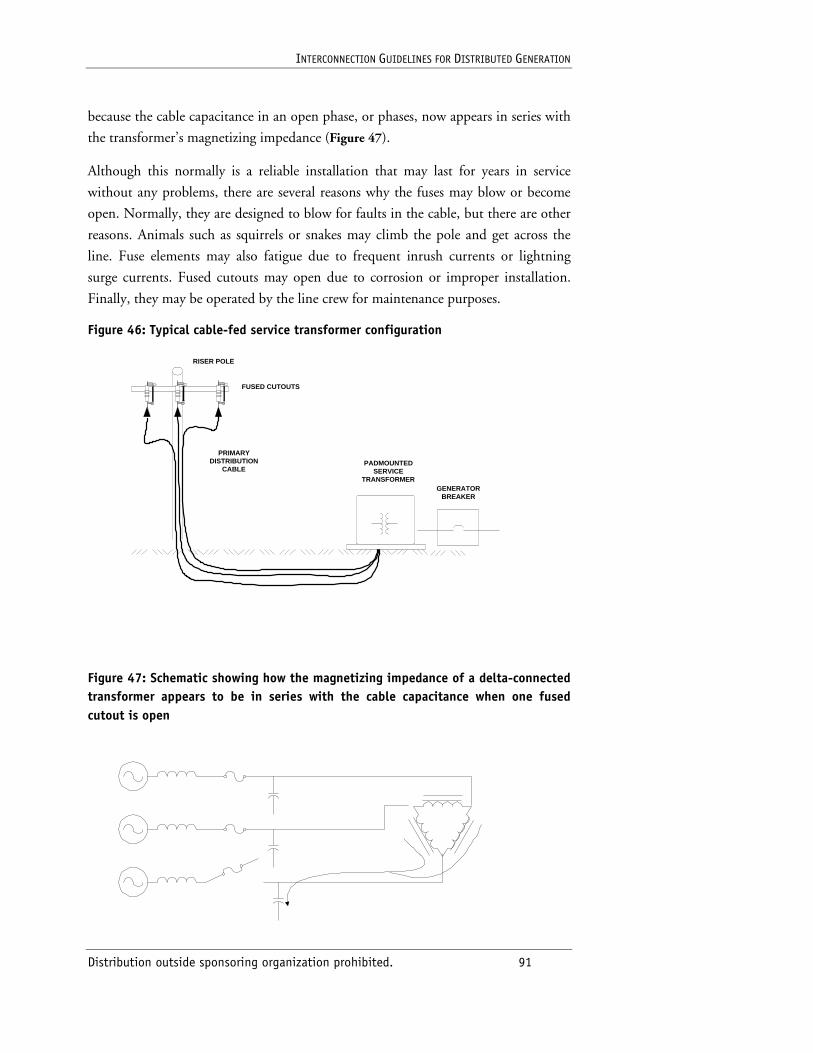
INTERCONNECTION GUIDELINES FOR DISTRIBUTED GENERATION
Distribution outside sponsoring organization prohibited. 91
because the cable capacitance in an open phase, or phases, now appears in series with
the transformer’s magnetizing impedance (Figure 47).
Although this normally is a reliable installation that may last for years in service
without any problems, there are several reasons why the fuses may blow or become
open. Normally, they are designed to blow for faults in the cable, but there are other
reasons. Animals such as squirrels or snakes may climb the pole and get across the
line. Fuse elements may also fatigue due to frequent inrush currents or lightning
surge currents. Fused cutouts may open due to corrosion or improper installation.
Finally, they may be operated by the line crew for maintenance purposes.
Figure 46: Typical cable-fed service transformer configuration
Figure 47: Schematic showing how the magnetizing impedance of a delta-connected transformer appears to be in series with the cable capacitance when one fused cutout is open
PADMOUNTEDSERVICE
TRANSFORMERGENERATOR
BREAKER
PRIMARYDISTRIBUTION
CABLE
FUSED CUTOUTS
RISER POLE
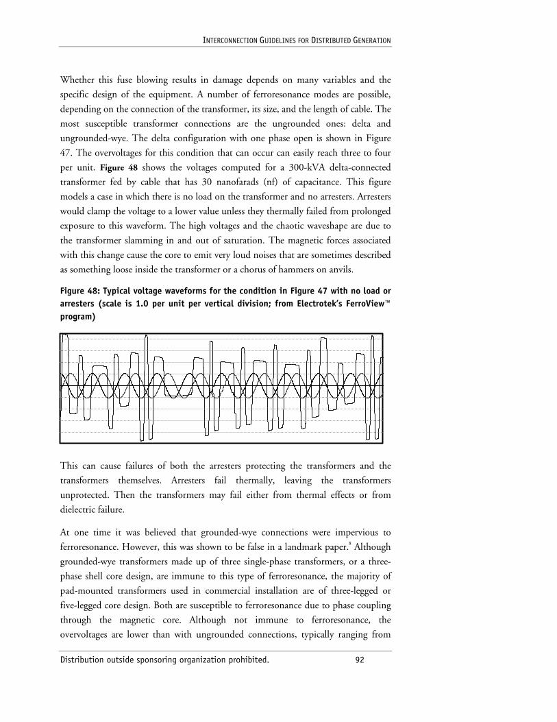
INTERCONNECTION GUIDELINES FOR DISTRIBUTED GENERATION
Distribution outside sponsoring organization prohibited. 92
Whether this fuse blowing results in damage depends on many variables and the
specific design of the equipment. A number of ferroresonance modes are possible,
depending on the connection of the transformer, its size, and the length of cable. The
most susceptible transformer connections are the ungrounded ones: delta and
ungrounded-wye. The delta configuration with one phase open is shown in Figure
47. The overvoltages for this condition that can occur can easily reach three to four
per unit. Figure 48 shows the voltages computed for a 300-kVA delta-connected
transformer fed by cable that has 30 nanofarads (nf) of capacitance. This figure
models a case in which there is no load on the transformer and no arresters. Arresters
would clamp the voltage to a lower value unless they thermally failed from prolonged
exposure to this waveform. The high voltages and the chaotic waveshape are due to
the transformer slamming in and out of saturation. The magnetic forces associated
with this change cause the core to emit very loud noises that are sometimes described
as something loose inside the transformer or a chorus of hammers on anvils.
Figure 48: Typical voltage waveforms for the condition in Figure 47 with no load or arresters (scale is 1.0 per unit per vertical division; from Electrotek’s FerroView™ program)
This can cause failures of both the arresters protecting the transformers and the
transformers themselves. Arresters fail thermally, leaving the transformers
unprotected. Then the transformers may fail either from thermal effects or from
dielectric failure.
At one time it was believed that grounded-wye connections were impervious to
ferroresonance. However, this was shown to be false in a landmark paper.8 Although
grounded-wye transformers made up of three single-phase transformers, or a three-
phase shell core design, are immune to this type of ferroresonance, the majority of
pad-mounted transformers used in commercial installation are of three-legged or
five-legged core design. Both are susceptible to ferroresonance due to phase coupling
through the magnetic core. Although not immune to ferroresonance, the
overvoltages are lower than with ungrounded connections, typically ranging from
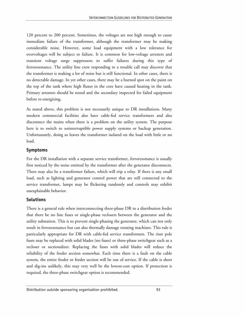
INTERCONNECTION GUIDELINES FOR DISTRIBUTED GENERATION
Distribution outside sponsoring organization prohibited. 93
120 percent to 200 percent. Sometimes, the voltages are not high enough to cause
immediate failure of the transformer, although the transformer may be making
considerable noise. However, some load equipment with a low tolerance for
overvoltages will be subject to failure. It is common for low-voltage arresters and
transient voltage surge suppressors to suffer failures during this type of
ferroresonance. The utility line crew responding to a trouble call may discover that
the transformer is making a lot of noise but is still functional. In other cases, there is
no detectable damage. In yet other cases, there may be a burned spot on the paint on
the top of the tank where high fluxes in the core have caused heating in the tank.
Primary arresters should be tested and the secondary inspected for failed equipment
before re-energizing.
As stated above, this problem is not necessarily unique to DR installations. Many
modern commercial facilities also have cable-fed service transformers and also
disconnect the mains when there is a problem on the utility system. The purpose
here is to switch to uninterruptible power supply systems or backup generation.
Unfortunately, doing so leaves the transformer isolated on the load with little or no
load.
Symptoms
For the DR installation with a separate service transformer, ferroresonance is usually
first noticed by the noise emitted by the transformer after the generator disconnects.
There may also be a transformer failure, which will trip a relay. If there is any small
load, such as lighting and generator control power that are still connected to the
service transformer, lamps may be flickering randomly and controls may exhibit
unexplainable behavior.
Solutions
There is a general rule when interconnecting three-phase DR to a distribution feeder
that there be no line fuses or single-phase reclosers between the generator and the
utility substation. This is to prevent single-phasing the generator, which can not only
result in ferroresonance but can also thermally damage rotating machines. This rule is
particularly appropriate for DR with cable-fed service transformers. The riser pole
fuses may be replaced with solid blades (no fuses) or three-phase switchgear such as a
recloser or sectionalizer. Replacing the fuses with solid blades will reduce the
reliability of the feeder section somewhat. Each time there is a fault on the cable
system, the entire feeder or feeder section will be out of service. If the cable is short
and dig-ins unlikely, this may very well be the lowest-cost option. If protection is
required, the three-phase switchgear option is recommended.
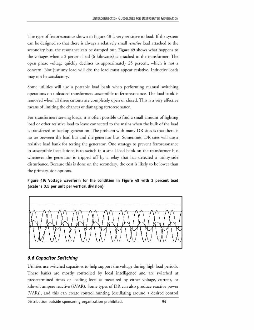
INTERCONNECTION GUIDELINES FOR DISTRIBUTED GENERATION
Distribution outside sponsoring organization prohibited. 94
The type of ferroresonance shown in Figure 48 is very sensitive to load. If the system
can be designed so that there is always a relatively small resistive load attached to the
secondary bus, the resonance can be damped out. Figure 49 shows what happens to
the voltages when a 2 percent load (6 kilowatts) is attached to the transformer. The
open phase voltage quickly declines to approximately 25 percent, which is not a
concern. Not just any load will do: the load must appear resistive. Inductive loads
may not be satisfactory.
Some utilities will use a portable load bank when performing manual switching
operations on unloaded transformers susceptible to ferroresonance. The load bank is
removed when all three cutouts are completely open or closed. This is a very effective
means of limiting the chances of damaging ferroresonance.
For transformers serving loads, it is often possible to find a small amount of lighting
load or other resistive load to leave connected to the mains when the bulk of the load
is transferred to backup generation. The problem with many DR sites is that there is
no tie between the load bus and the generator bus. Sometimes, DR sites will use a
resistive load bank for testing the generator. One strategy to prevent ferroresonance
in susceptible installations is to switch in a small load bank on the transformer bus
whenever the generator is tripped off by a relay that has detected a utility-side
disturbance. Because this is done on the secondary, the cost is likely to be lower than
the primary-side options.
Figure 49: Voltage waveform for the condition in Figure 48 with 2 percent load (scale is 0.5 per unit per vertical division)
6.6 Capacitor Switching
Utilities use switched capacitors to help support the voltage during high load periods.
These banks are mostly controlled by local intelligence and are switched at
predetermined times or loading level as measured by either voltage, current, or
kilovolt ampere reactive (kVAR). Some types of DR can also produce reactive power
(VARs), and this can create control hunting (oscillating around a desired control
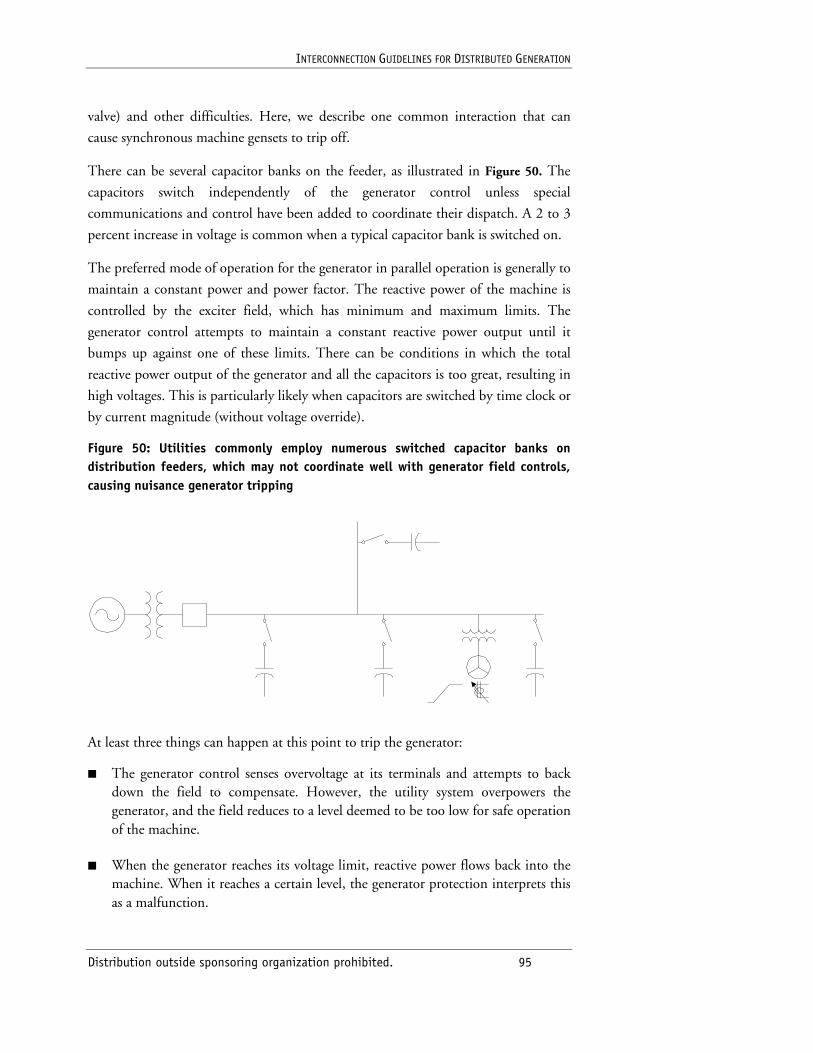
INTERCONNECTION GUIDELINES FOR DISTRIBUTED GENERATION
Distribution outside sponsoring organization prohibited. 95
valve) and other difficulties. Here, we describe one common interaction that can
cause synchronous machine gensets to trip off.
There can be several capacitor banks on the feeder, as illustrated in Figure 50. The
capacitors switch independently of the generator control unless special
communications and control have been added to coordinate their dispatch. A 2 to 3
percent increase in voltage is common when a typical capacitor bank is switched on.
The preferred mode of operation for the generator in parallel operation is generally to
maintain a constant power and power factor. The reactive power of the machine is
controlled by the exciter field, which has minimum and maximum limits. The
generator control attempts to maintain a constant reactive power output until it
bumps up against one of these limits. There can be conditions in which the total
reactive power output of the generator and all the capacitors is too great, resulting in
high voltages. This is particularly likely when capacitors are switched by time clock or
by current magnitude (without voltage override).
Figure 50: Utilities commonly employ numerous switched capacitor banks on distribution feeders, which may not coordinate well with generator field controls, causing nuisance generator tripping
At least three things can happen at this point to trip the generator:
■ The generator control senses overvoltage at its terminals and attempts to back down the field to compensate. However, the utility system overpowers the generator, and the field reduces to a level deemed to be too low for safe operation of the machine.
■ When the generator reaches its voltage limit, reactive power flows back into the machine. When it reaches a certain level, the generator protection interprets this as a malfunction.
INTERCONNECTION GUIDELINES FOR DISTRIBUTED GENERATION
Distribution outside sponsoring organization prohibited. 96
■ DR technologies not capable of producing reactive power (some inverter interfaces) trip on overvoltage.
Symptoms
The chief symptom will be that the DR trips off line frequently—perhaps as often as
once a day. Tripping may also occur at the same time each day, which is a clear
indication of a miscoordination between the DR and a time-controlled capacitor
bank. Tripping may occur only on weekends, when the load is low and system
voltages tend to run high.
Solutions
■ One solution is to change the tap on the service transformer to reduce the voltage at the generator terminals.
■ It may be possible with appropriate communications and control to inhibit the switching of certain capacitors when a generator is running. The utility may also choose to simply remove a capacitor from service and rely on the DR to produce the reactive power. The DR technology would have to be appropriate for the application and must be likely to be on line when needed.
■ Problematic machines may be replaced with less-susceptible ones. There is variability in the excitation capabilities of synchronous machines, and some are more tolerant of operating at low field levels or at negative power factor.
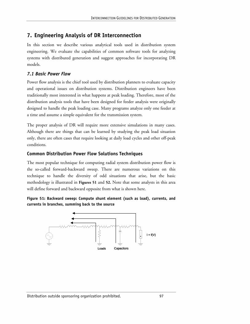
INTERCONNECTION GUIDELINES FOR DISTRIBUTED GENERATION
Distribution outside sponsoring organization prohibited. 97
7. Engineering Analysis of DR Interconnection
In this section we describe various analytical tools used in distribution system
engineering. We evaluate the capabilities of common software tools for analyzing
systems with distributed generation and suggest approaches for incorporating DR
models.
7.1 Basic Power Flow
Power flow analysis is the chief tool used by distribution planners to evaluate capacity
and operational issues on distribution systems. Distribution engineers have been
traditionally most interested in what happens at peak loading. Therefore, most of the
distribution analysis tools that have been designed for feeder analysis were originally
designed to handle the peak loading case. Many programs analyze only one feeder at
a time and assume a simple equivalent for the transmission system.
The proper analysis of DR will require more extensive simulations in many cases.
Although there are things that can be learned by studying the peak load situation
only, there are often cases that require looking at daily load cycles and other off-peak
conditions.
Common Distribution Power Flow Solutions Techniques
The most popular technique for computing radial system distribution power flow is
the so-called forward-backward sweep. There are numerous variations on this
technique to handle the diversity of odd situations that arise, but the basic
methodology is illustrated in Figures 51 and 52. Note that some analysts in this area
will define forward and backward opposite from what is shown here.
Figure 51: Backward sweep: Compute shunt element (such as load), currents, and currents in branches, summing back to the source
I = f(V)
Loads Capacitors
I = f(V)
Loads Capacitors
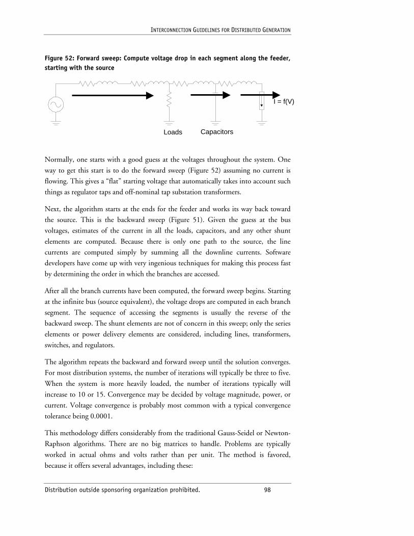
INTERCONNECTION GUIDELINES FOR DISTRIBUTED GENERATION
Distribution outside sponsoring organization prohibited. 98
Figure 52: Forward sweep: Compute voltage drop in each segment along the feeder, starting with the source
I = f(V)
Loads Capacitors
Normally, one starts with a good guess at the voltages throughout the system. One
way to get this start is to do the forward sweep (Figure 52) assuming no current is
flowing. This gives a “flat” starting voltage that automatically takes into account such
things as regulator taps and off-nominal tap substation transformers.
Next, the algorithm starts at the ends for the feeder and works its way back toward
the source. This is the backward sweep (Figure 51). Given the guess at the bus
voltages, estimates of the current in all the loads, capacitors, and any other shunt
elements are computed. Because there is only one path to the source, the line
currents are computed simply by summing all the downline currents. Software
developers have come up with very ingenious techniques for making this process fast
by determining the order in which the branches are accessed.
After all the branch currents have been computed, the forward sweep begins. Starting
at the infinite bus (source equivalent), the voltage drops are computed in each branch
segment. The sequence of accessing the segments is usually the reverse of the
backward sweep. The shunt elements are not of concern in this sweep; only the series
elements or power delivery elements are considered, including lines, transformers,
switches, and regulators.
The algorithm repeats the backward and forward sweep until the solution converges.
For most distribution systems, the number of iterations will typically be three to five.
When the system is more heavily loaded, the number of iterations typically will
increase to 10 or 15. Convergence may be decided by voltage magnitude, power, or
current. Voltage convergence is probably most common with a typical convergence
tolerance being 0.0001.
This methodology differs considerably from the traditional Gauss-Seidel or Newton-
Raphson algorithms. There are no big matrices to handle. Problems are typically
worked in actual ohms and volts rather than per unit. The method is favored,
because it offers several advantages, including these:
INTERCONNECTION GUIDELINES FOR DISTRIBUTED GENERATION
Distribution outside sponsoring organization prohibited. 99
■ Speed is probably the greatest advantage to developers of distribution analysis software. This method is much faster than power flow methods designed for large meshed networks. Speed is nearly linearly proportional to problem size, allowing very large radial systems to be solved in seconds.
■ Sequencing of the voltage regulation devices (regulators) and capacitors falls out naturally from the sweep algorithm.
■ A wide range of load models and models of other shunt elements is easily handled. These elements are basically treated as current injection sources into the power delivery network.
This method falls into the general class of point-Jacobi methods for solving nonlinear
equations. As such, there are some limitations to the range of values for which the
solution will converge. To summarize briefly, the limitations basically boil down to
meaning that the apparent impedance of all the shunt-connected elements must
always be greater than the impedance of all the series elements. Quite a strain is put
on the convergence of this method when the voltage drops below 80 percent. The
lower limit is generally around 70 percent. This is not a concern for power flow
calculations where we expect the voltages to be greater than 90 percent. However, it
means that this method of solution is restricted to power flows and cannot be used
for short-circuit calculations or harmonics analysis.
Developers have been quite creative in working around these limitations. Some
models will automatically change to a linear element during the solution process so
that convergence can be achieved at low voltages.
This method does not apply directly to network circuits. However, many
distribution systems have spot networks or other weakly meshed systems. When there
are not many loops in the system, these can be analyzed with radial system
algorithms by using a few tricks.9 One simple one is shown in Figure 53. The
network is broken in a selected location and the loop tie replaced with equal and
opposite current injection sources. The system topology reverts to radial, allowing
the radial solution algorithm process to be used. The iteration process is modified to
enforce the Kirchoff constraints at the break point as closely as possible.
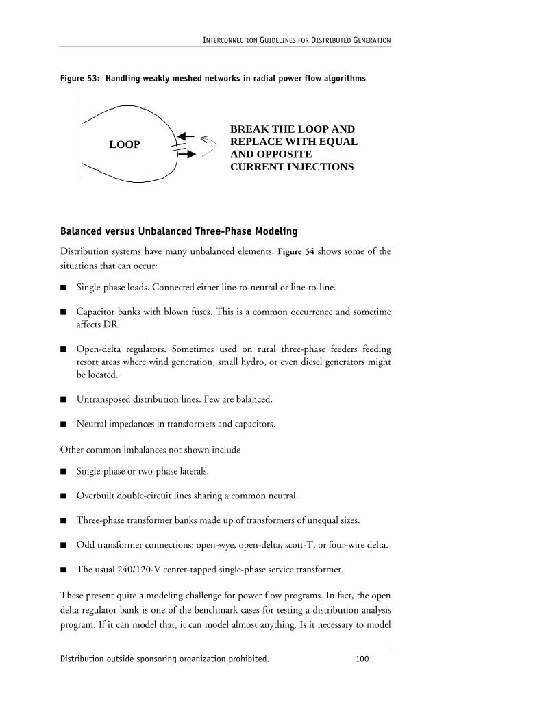
INTERCONNECTION GUIDELINES FOR DISTRIBUTED GENERATION
Distribution outside sponsoring organization prohibited. 100
Figure 53: Handling weakly meshed networks in radial power flow algorithms
LOOP BREAK THE LOOP AND REPLACE WITH EQUAL AND OPPOSITE CURRENT INJECTIONS
Balanced versus Unbalanced Three-Phase Modeling
Distribution systems have many unbalanced elements. Figure 54 shows some of the
situations that can occur:
■ Single-phase loads. Connected either line-to-neutral or line-to-line.
■ Capacitor banks with blown fuses. This is a common occurrence and sometime affects DR.
■ Open-delta regulators. Sometimes used on rural three-phase feeders feeding resort areas where wind generation, small hydro, or even diesel generators might be located.
■ Untransposed distribution lines. Few are balanced.
■ Neutral impedances in transformers and capacitors.
Other common imbalances not shown include
■ Single-phase or two-phase laterals.
■ Overbuilt double-circuit lines sharing a common neutral.
■ Three-phase transformer banks made up of transformers of unequal sizes.
■ Odd transformer connections: open-wye, open-delta, scott-T, or four-wire delta.
■ The usual 240/120-V center-tapped single-phase service transformer.
These present quite a modeling challenge for power flow programs. In fact, the open
delta regulator bank is one of the benchmark cases for testing a distribution analysis
program. If it can model that, it can model almost anything. Is it necessary to model
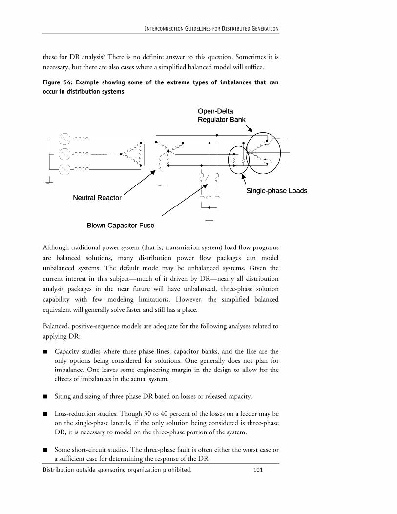
INTERCONNECTION GUIDELINES FOR DISTRIBUTED GENERATION
Distribution outside sponsoring organization prohibited. 101
these for DR analysis? There is no definite answer to this question. Sometimes it is
necessary, but there are also cases where a simplified balanced model will suffice.
Figure 54: Example showing some of the extreme types of imbalances that can occur in distribution systems
Although traditional power system (that is, transmission system) load flow programs
are balanced solutions, many distribution power flow packages can model
unbalanced systems. The default mode may be unbalanced systems. Given the
current interest in this subject—much of it driven by DR—nearly all distribution
analysis packages in the near future will have unbalanced, three-phase solution
capability with few modeling limitations. However, the simplified balanced
equivalent will generally solve faster and still has a place.
Balanced, positive-sequence models are adequate for the following analyses related to
applying DR:
■ Capacity studies where three-phase lines, capacitor banks, and the like are the only options being considered for solutions. One generally does not plan for imbalance. One leaves some engineering margin in the design to allow for the effects of imbalances in the actual system.
■ Siting and sizing of three-phase DR based on losses or released capacity.
■ Loss-reduction studies. Though 30 to 40 percent of the losses on a feeder may be on the single-phase laterals, if the only solution being considered is three-phase DR, it is necessary to model on the three-phase portion of the system.
■ Some short-circuit studies. The three-phase fault is often either the worst case or a sufficient case for determining the response of the DR.
Blown Capacitor Fuse
Neutral ReactorSingle-phase Loads
Open-Delta Regulator Bank
Blown Capacitor Fuse
Neutral ReactorSingle-phase Loads
Open-Delta Regulator Bank
INTERCONNECTION GUIDELINES FOR DISTRIBUTED GENERATION
Distribution outside sponsoring organization prohibited. 102
■ Some islanding studies. Normally, this is done by opening a three-phase switch or breaker and determining how quickly the voltage and frequency deviate from normal. If this shows a high potential for islanding, it might be worthwhile to then build an unbalanced model and add single-phase loads. Some DR will have difficulty serving an unbalanced load, and that would not show up in a balanced dynamics analysis.
■ Some reliability studies.
Unbalanced models are necessary for the following:
■ Designing or operating close to the feeder current and voltage limits. Imbalances can create significant difference between the phases.
■ Modeling long single-phase or two-phase laterals.
■ Studying high penetrations of single-phase DR.
■ Detailed short studies to determine what the DR protective relaying will see for unbalanced utility-side faults.
■ Determining dynamic or other response of DR to unbalanced utility faults (80 to 90 percent will be single-line-to-ground faults).
■ Voltage fluctuation studies for wind generation fed from long, untransposed feeders with single-phase regulators.
■ Other voltage regulator studies (voltage regulators are usually operated as independent, single-phase devices).
■ Accurate and realistic harmonics studies.
■ Switching transients, ferroresonance, and other resonance studies.
■ Accurate reliability studies.
Modeling DR for Distribution Power Flow Analysis
In the forward/backward sweep method, DR is typically treated as another current
injection source. That is, it behaves like a negative load. This is exactly the way most
DR will behave when interconnected. Generally, the exciter controls on synchronous
machines are set to hold constant reactive power or power factor. Inverters are often
factory set to produce only unity power factor while they are in utility-interactive
mode. Therefore, this model will suffice for most DR analysis.
INTERCONNECTION GUIDELINES FOR DISTRIBUTED GENERATION
Distribution outside sponsoring organization prohibited. 103
Because most distribution power flow methods were designed for systems with only
one source, the modeling of DR that actively regulates the bus voltage is more
difficult. The methods do not naturally accept the so-called “P-V” bus model, where
power and voltage magnitude are the given quantities. However, a few commercial
packages have implemented modifications to their algorithms to accomplish this, and
it is expected that more will be able to model such DR soon.
This issue would apply to large generation that actually has the capacity to control
the utility bus voltage. There are a few instances where the utility may prefer this
type of operation. One example is a generator located several miles from the
substation where the system is weak and the load is not constant. The generator may
be able to do a better job of regulating the voltage than other options. However, this
ability comes with a price. While operating in automatic voltage regulation (AVR)
mode, the generator is much more likely to sustain an island. Therefore, the anti-
islanding detection is more expensive.
Determining DR Capacity Impacts
The potential benefits of DR are very time- and location-specific. That is, the value
varies according to where the DR is located and when it is operating. If the utility is
considering offering capacity credits, it is important to determine if the subject DR
has any real value to the system. For some applications, this is difficult to judge from
just a snapshot power flow solution of a peak load condition. The solution must be
performed over a period of time to determine such things as the number of hours the
generator is likely to run and the cumulative benefit to the system.
The ability to follow a daily load profile such as the one shown in Figure 55 has not
been a traditional part of power flow packages for either transmission or distribution
systems. There is quite a lot of variation in the ability of the different commercial
packages to accommodate this. However, it is often very important for analysis of
both peaking DR and base-load cogeneration. For example, the voltage regulators
and capacitors are designed to operate in a particular sequence, and the best way to
simulate that is to perform power flow solutions following the daily load curve. It is
difficult to get the correct answer with a single snapshot.
The other issue is finding a location where DR is beneficial and measuring the
benefit. Figure 56 illustrates one situation. Here the benefit is measured in terms of
the additional amount of load that can be served by a feeder relative to the size of the
DR added. This measure is popular in some transmission planning studies. In this
case the constraint is assumed to be in the feeder. This would typically be either low
voltage toward the ends of the feeder or excessive current in some line or transformer.
DR is of no value unless it can relieve that constraint. Therefore, if the DR is located
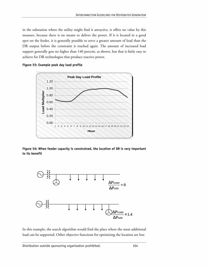
INTERCONNECTION GUIDELINES FOR DISTRIBUTED GENERATION
Distribution outside sponsoring organization prohibited. 104
in the substation where the utility might find it attractive, it offers no value by this
measure, because there is no means to deliver the power. If it is located in a good
spot on the feeder, it is generally possible to serve a greater amount of load than the
DR output before the constraint is reached again. The amount of increased load
support generally gets no higher than 140 percent, as shown, but that is fairly easy to
achieve for DR technologies that produce reactive power.
Figure 55: Example peak day load profile
Peak Day Load Profile
0.00
0.20
0.40
0.60
0.80
1.00
1.20
1 2 3 4 5 6 7 8 9 10 11 12 13 14 15 16 17 18 19 20 21 22 23 24
Hour
Lo
ad M
ult
iplie
r
Figure 56: When feeder capacity is constrained, the location of DR is very important to its benefit
0=∆∆
GEN
LOAD
P
P
4.1=∆∆
GEN
LOAD
P
P
0=∆∆
GEN
LOAD
P
P
4.1=∆∆
GEN
LOAD
P
P
In this example, the search algorithm would find the place where the most additional
load can be supported. Other objective functions for optimizing the location are loss
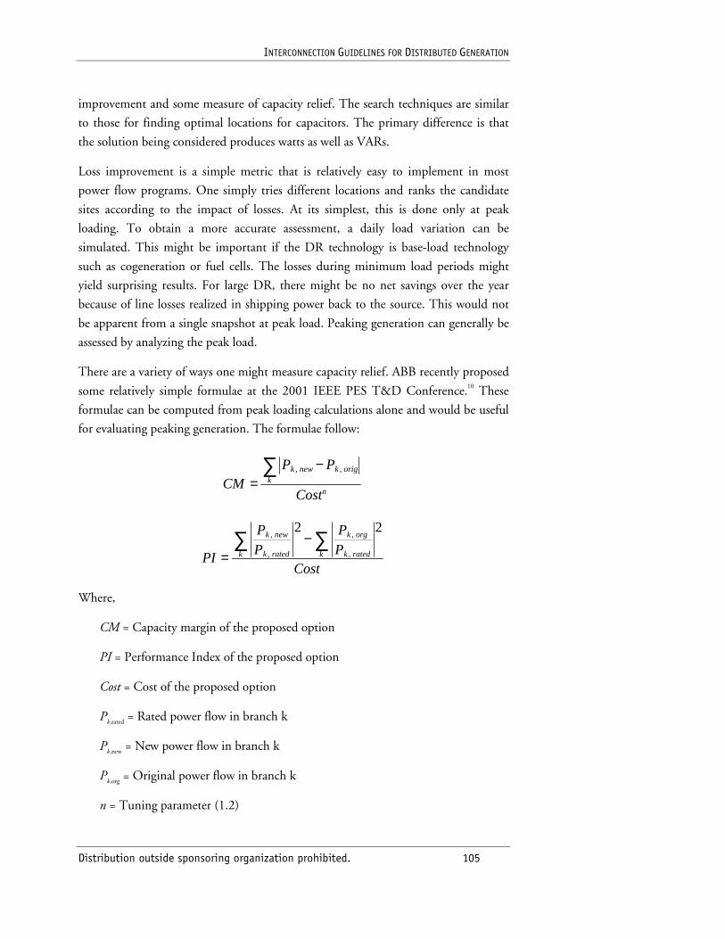
INTERCONNECTION GUIDELINES FOR DISTRIBUTED GENERATION
Distribution outside sponsoring organization prohibited. 105
improvement and some measure of capacity relief. The search techniques are similar
to those for finding optimal locations for capacitors. The primary difference is that
the solution being considered produces watts as well as VARs.
Loss improvement is a simple metric that is relatively easy to implement in most
power flow programs. One simply tries different locations and ranks the candidate
sites according to the impact of losses. At its simplest, this is done only at peak
loading. To obtain a more accurate assessment, a daily load variation can be
simulated. This might be important if the DR technology is base-load technology
such as cogeneration or fuel cells. The losses during minimum load periods might
yield surprising results. For large DR, there might be no net savings over the year
because of line losses realized in shipping power back to the source. This would not
be apparent from a single snapshot at peak load. Peaking generation can generally be
assessed by analyzing the peak load.
There are a variety of ways one might measure capacity relief. ABB recently proposed
some relatively simple formulae at the 2001 IEEE PES T&D Conference.10 These
formulae can be computed from peak loading calculations alone and would be useful
for evaluating peaking generation. The formulae follow:
Where,
CM = Capacity margin of the proposed option
PI = Performance Index of the proposed option
Cost = Cost of the proposed option
Pk,rated = Rated power flow in branch k
Pk,new = New power flow in branch k
Pk,org = Original power flow in branch k
n = Tuning parameter (1.2)
nk
origknewk
Cost
PPCM
∑ −=
,,
CostP
P
P
P
PI k ratedk
orgk
k ratedk
newk ∑∑ −=
22
,
,
,
,
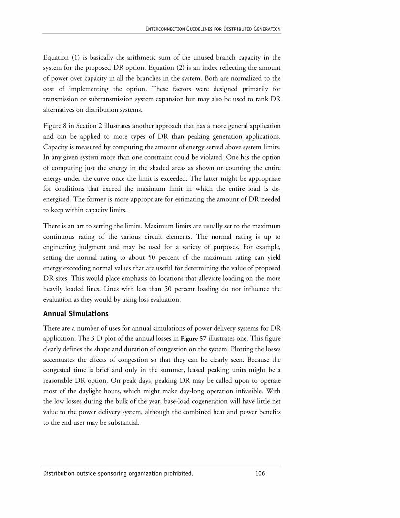
INTERCONNECTION GUIDELINES FOR DISTRIBUTED GENERATION
Distribution outside sponsoring organization prohibited. 106
Equation (1) is basically the arithmetic sum of the unused branch capacity in the
system for the proposed DR option. Equation (2) is an index reflecting the amount
of power over capacity in all the branches in the system. Both are normalized to the
cost of implementing the option. These factors were designed primarily for
transmission or subtransmission system expansion but may also be used to rank DR
alternatives on distribution systems.
Figure 8 in Section 2 illustrates another approach that has a more general application
and can be applied to more types of DR than peaking generation applications.
Capacity is measured by computing the amount of energy served above system limits.
In any given system more than one constraint could be violated. One has the option
of computing just the energy in the shaded areas as shown or counting the entire
energy under the curve once the limit is exceeded. The latter might be appropriate
for conditions that exceed the maximum limit in which the entire load is de-
energized. The former is more appropriate for estimating the amount of DR needed
to keep within capacity limits.
There is an art to setting the limits. Maximum limits are usually set to the maximum
continuous rating of the various circuit elements. The normal rating is up to
engineering judgment and may be used for a variety of purposes. For example,
setting the normal rating to about 50 percent of the maximum rating can yield
energy exceeding normal values that are useful for determining the value of proposed
DR sites. This would place emphasis on locations that alleviate loading on the more
heavily loaded lines. Lines with less than 50 percent loading do not influence the
evaluation as they would by using loss evaluation.
Annual Simulations
There are a number of uses for annual simulations of power delivery systems for DR
application. The 3-D plot of the annual losses in Figure 57 illustrates one. This figure
clearly defines the shape and duration of congestion on the system. Plotting the losses
accentuates the effects of congestion so that they can be clearly seen. Because the
congested time is brief and only in the summer, leased peaking units might be a
reasonable DR option. On peak days, peaking DR may be called upon to operate
most of the daylight hours, which might make day-long operation infeasible. With
the low losses during the bulk of the year, base-load cogeneration will have little net
value to the power delivery system, although the combined heat and power benefits
to the end user may be substantial.
INTERCONNECTION GUIDELINES FOR DISTRIBUTED GENERATION
Distribution outside sponsoring organization prohibited. 107
Figure 57: Annual distribution system loss characteristics
1
5
9
13
17
21
Jan Apr Ju
l
Oct
0
5000
10000
15000
20000
25000
kWh
Hour
Month
One strategy for performing annual load simulations is to simply compute 8,760
hourly power flow solutions sequentially. This is accurate but can be time-consuming
for larger circuits. Figure 58 shows a typical characteristic for the peak load of each
day of the year. This was extracted from an 8,760-hour data stream recorded for the
actual load. Modern metering equipment is making this data relatively easy to
obtain.
The 8,760-hour data may be easily distilled into a load-duration curve by sorting the
hourly data in order (Figure 59). This is almost always a smooth curve that can be
fitted accurately with a few straight lines. Therefore, an annual simulation of energy
quantities can be determined quickly by only a few power flow solutions. This is
generally used only for gross estimates of annual performance but does have several
uses for DR analysis. Combining the load-duration curve with the daily load shape
can improve accuracy, especially for the simulation of peaking generation, in which it
is important to properly sequence the regulators and capacitors. A useful annual
simulation may be obtained from approximately 150 power flow solutions.
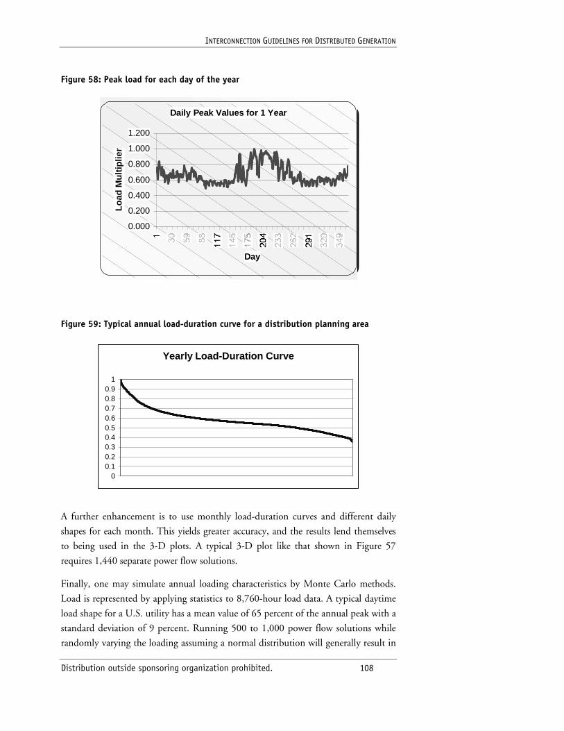
INTERCONNECTION GUIDELINES FOR DISTRIBUTED GENERATION
Distribution outside sponsoring organization prohibited. 108
Figure 58: Peak load for each day of the year
Figure 59: Typical annual load-duration curve for a distribution planning area
Yearly Load-Duration Curve
00.10.20.30.40.50.60.70.80.9
1
A further enhancement is to use monthly load-duration curves and different daily
shapes for each month. This yields greater accuracy, and the results lend themselves
to being used in the 3-D plots. A typical 3-D plot like that shown in Figure 57
requires 1,440 separate power flow solutions.
Finally, one may simulate annual loading characteristics by Monte Carlo methods.
Load is represented by applying statistics to 8,760-hour load data. A typical daytime
load shape for a U.S. utility has a mean value of 65 percent of the annual peak with a
standard deviation of 9 percent. Running 500 to 1,000 power flow solutions while
randomly varying the loading assuming a normal distribution will generally result in
Daily Peak Values for 1 Year
0.000
0.200
0.400
0.600
0.800
1.000
1.200
Day
Lo
ad M
ult
iplie
r
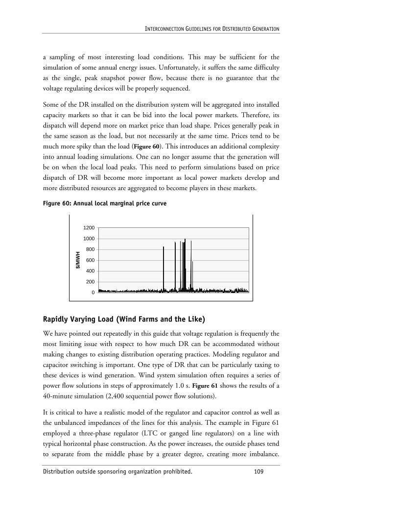
INTERCONNECTION GUIDELINES FOR DISTRIBUTED GENERATION
Distribution outside sponsoring organization prohibited. 109
a sampling of most interesting load conditions. This may be sufficient for the
simulation of some annual energy issues. Unfortunately, it suffers the same difficulty
as the single, peak snapshot power flow, because there is no guarantee that the
voltage regulating devices will be properly sequenced.
Some of the DR installed on the distribution system will be aggregated into installed
capacity markets so that it can be bid into the local power markets. Therefore, its
dispatch will depend more on market price than load shape. Prices generally peak in
the same season as the load, but not necessarily at the same time. Prices tend to be
much more spiky than the load (Figure 60). This introduces an additional complexity
into annual loading simulations. One can no longer assume that the generation will
be on when the local load peaks. This need to perform simulations based on price
dispatch of DR will become more important as local power markets develop and
more distributed resources are aggregated to become players in these markets.
Figure 60: Annual local marginal price curve
0
200
400
600
800
1000
1200
$/M
WH
Rapidly Varying Load (Wind Farms and the Like)
We have pointed out repeatedly in this guide that voltage regulation is frequently the
most limiting issue with respect to how much DR can be accommodated without
making changes to existing distribution operating practices. Modeling regulator and
capacitor switching is important. One type of DR that can be particularly taxing to
these devices is wind generation. Wind system simulation often requires a series of
power flow solutions in steps of approximately 1.0 s. Figure 61 shows the results of a
40-minute simulation (2,400 sequential power flow solutions).
It is critical to have a realistic model of the regulator and capacitor control as well as
the unbalanced impedances of the lines for this analysis. The example in Figure 61
employed a three-phase regulator (LTC or ganged line regulators) on a line with
typical horizontal phase construction. As the power increases, the outside phases tend
to separate from the middle phase by a greater degree, creating more imbalance.
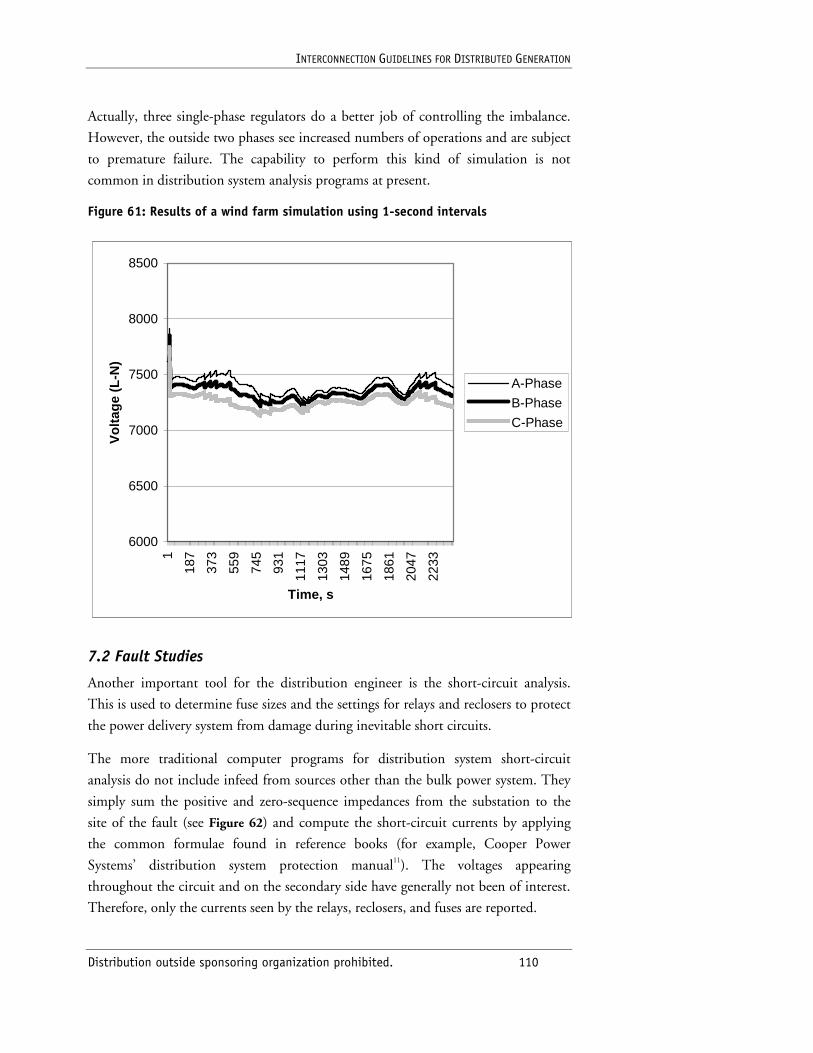
INTERCONNECTION GUIDELINES FOR DISTRIBUTED GENERATION
Distribution outside sponsoring organization prohibited. 110
Actually, three single-phase regulators do a better job of controlling the imbalance.
However, the outside two phases see increased numbers of operations and are subject
to premature failure. The capability to perform this kind of simulation is not
common in distribution system analysis programs at present.
Figure 61: Results of a wind farm simulation using 1-second intervals
6000
6500
7000
7500
8000
8500
1
187
373
559
745
931
1117
1303
1489
1675
1861
2047
2233
Time, s
Vo
ltag
e (L
-N)
A-Phase
B-Phase
C-Phase
7.2 Fault Studies
Another important tool for the distribution engineer is the short-circuit analysis.
This is used to determine fuse sizes and the settings for relays and reclosers to protect
the power delivery system from damage during inevitable short circuits.
The more traditional computer programs for distribution system short-circuit
analysis do not include infeed from sources other than the bulk power system. They
simply sum the positive and zero-sequence impedances from the substation to the
site of the fault (see Figure 62) and compute the short-circuit currents by applying
the common formulae found in reference books (for example, Cooper Power
Systems’ distribution system protection manual11). The voltages appearing
throughout the circuit and on the secondary side have generally not been of interest.
Therefore, only the currents seen by the relays, reclosers, and fuses are reported.
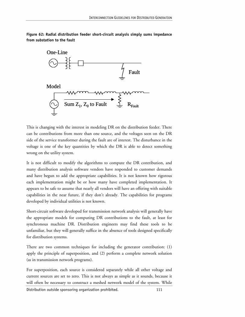
INTERCONNECTION GUIDELINES FOR DISTRIBUTED GENERATION
Distribution outside sponsoring organization prohibited. 111
Figure 62: Radial distribution feeder short-circuit analysis simply sums impedance from substation to the fault
RFault
Model
One-Line
Fault
Sum Z1, Z0 to Fault RFault
Model
One-Line
Fault
Sum Z1, Z0 to Fault
This is changing with the interest in modeling DR on the distribution feeder. There
can be contributions from more than one source, and the voltages seen on the DR
side of the service transformer during the fault are of interest. The disturbance in the
voltage is one of the key quantities by which the DR is able to detect something
wrong on the utility system.
It is not difficult to modify the algorithms to compute the DR contribution, and
many distribution analysis software vendors have responded to customer demands
and have begun to add the appropriate capabilities. It is not known how rigorous
each implementation might be or how many have completed implementation. It
appears to be safe to assume that nearly all vendors will have an offering with suitable
capabilities in the near future, if they don’t already. The capabilities for programs
developed by individual utilities is not known.
Short-circuit software developed for transmission network analysis will generally have
the appropriate models for computing DR contributions to the fault, at least for
synchronous machine DR. Distribution engineers may find these tools to be
unfamiliar, but they will generally suffice in the absence of tools designed specifically
for distribution systems.
There are two common techniques for including the generator contribution: (1)
apply the principle of superposition, and (2) perform a complete network solution
(as in transmission network programs).
For superposition, each source is considered separately while all other voltage and
current sources are set to zero. This is not always as simple as it sounds, because it
will often be necessary to construct a meshed network model of the system. While
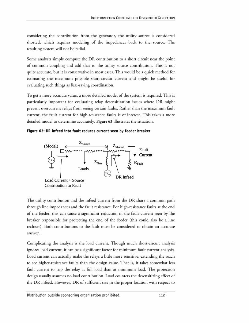
INTERCONNECTION GUIDELINES FOR DISTRIBUTED GENERATION
Distribution outside sponsoring organization prohibited. 112
considering the contribution from the generator, the utility source is considered
shorted, which requires modeling of the impedances back to the source. The
resulting system will not be radial.
Some analysts simply compute the DR contribution to a short circuit near the point
of common coupling and add that to the utility source contribution. This is not
quite accurate, but it is conservative in most cases. This would be a quick method for
estimating the maximum possible short-circuit current and might be useful for
evaluating such things as fuse-saving coordination.
To get a more accurate value, a more detailed model of the system is required. This is
particularly important for evaluating relay desensitization issues where DR might
prevent overcurrent relays from seeing certain faults. Rather than the maximum fault
current, the fault current for high-resistance faults is of interest. This takes a more
detailed model to determine accurately. Figure 63 illustrates the situation.
Figure 63: DR infeed into fault reduces current seen by feeder breaker
RFault
(Model)
Loads
ZSource
ZGen
ZShared
DR InfeedLoad Current + Source Contribution to Fault
Fault Current
RFault
(Model)
Loads
ZSource
ZGen
ZShared
DR InfeedLoad Current + Source Contribution to Fault
Fault Current
The utility contribution and the infeed current from the DR share a common path
through line impedances and the fault resistance. For high-resistance faults at the end
of the feeder, this can cause a significant reduction in the fault current seen by the
breaker responsible for protecting the end of the feeder (this could also be a line
recloser). Both contributions to the fault must be considered to obtain an accurate
answer.
Complicating the analysis is the load current. Though much short-circuit analysis
ignores load current, it can be a significant factor for minimum fault current analysis.
Load current can actually make the relays a little more sensitive, extending the reach
to see higher-resistance faults than the design value. That is, it takes somewhat less
fault current to trip the relay at full load than at minimum load. The protection
design usually assumes no load contribution. Load counters the desensitizing effect of
the DR infeed. However, DR of sufficient size in the proper location with respect to
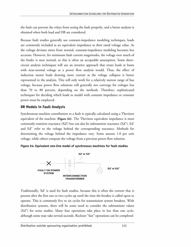
INTERCONNECTION GUIDELINES FOR DISTRIBUTED GENERATION
Distribution outside sponsoring organization prohibited. 113
the fault can prevent the relays from seeing the fault properly, and a better analysis is
obtained when both load and DR are considered.
Because fault studies generally use constant-impedance modeling techniques, loads
are commonly included as an equivalent impedance at their rated voltage value. As
the voltage deviates more from normal, constant-impedence modeling becomes less
accurate. However, for minimum fault current magnitudes, the voltage over much of
the feeder is near normal, so this is often an acceptable assumption. Some short-
circuit analysis techniques will use an iterative approach that treats loads at buses
with near-normal voltage as a power flow analysis would. Thus, the effect of
induction motor loads drawing more current as the voltage collapses is better
represented in the analysis. This will only work for a relatively narrow range of bus
voltage, because power flow solutions will generally not converge for voltages less
than 70 to 80 percent, depending on the methods. Therefore, sophisticated
techniques for deciding which loads to model with constant impedance or constant
power must be employed.
DR Models in Fault Analysis
Synchronous machine contribution to a fault is typically calculated using a Thevinen
equivalent of the machine (Figure 64). The Thevinen equivalent impedance is most
commonly transient reactance (Xd’) but can also be subtransient reactance (Xd"). Ed’
and Ed" refer to the voltage behind the corresponding reactance. Methods for
determining the voltage behind the impedance vary. Some assume 1.0 per unit
voltage, while others compute the voltage from a previous power flow solution.
Figure 64: Equivalent one-line model of synchronous machines for fault studies
Xd’ or Xd"
Ed’ or Ed"
INTERCONNECTIONTRANSFORMER
FAULT ON POWERSYSTEM
Traditionally, Xd’ is used for fault studies, because this is often the current that is
present after the first one or two cycles up until the time the breaker is called upon to
operate. This is commonly five to six cycles for transmission system breakers. With
distribution systems, there will be some need to consider the subtransient values
(Xd") for some studies. Many fuse operations take place in less than one cycle,
although some may take several seconds. Recloser “fast” operations can be completed
INTERCONNECTION GUIDELINES FOR DISTRIBUTED GENERATION
Distribution outside sponsoring organization prohibited. 114
in 1.5 cycles, although the rating may be 3 to 5 cycles. Using Xd" would give a more
accurate picture of the fault current and unfaulted phase voltages during those
conditions.
Induction machines introduce a need for engineering judgment. The textbook
picture of an induction machine subjected to a fault is that the fault current
contribution dies out very quickly in 1.5 cycles. The assumption is that the machine
was subjected to a three-phase fault at its terminals, causing the voltage to collapse.
This seldom happens in actual practice. Eighty to 90 percent of faults will be single-
phase faults for which the faulted phase voltage may exceed 0.5 per unit. The
excitation of the induction machine is only slightly diminished. The conservative
approach is to treat the induction machine as a synchronous machine for faults that
yield a high unfaulted phase voltage. The simple rule of thumb taught at the
University of Wisconsin-Madison Short Course on Interconnecting Distributed
Generation to the Distribution System is that the induction machine is treated as a
synchronous machine as long as the voltage exceeds 60 percent. If it is important to
get a precise number for the contribution, electromagnetic transients programs may
be used to model the induction machine in great detail.
IGBT inverters have limited capability to supply fault currents. When the controls
detect something wrong, they shut off immediately. One rule of thumb frequently
used by power systems analysts is to assume the inverter fault current contribution is
limited to 2.0 times normal rated current. Some utility engineers use 3.0 to be
conservative, but this is probably not warranted, because the contribution will
generally not be much greater than rated current. This can be a challenge to model in
short-circuit programs, because they usually do not have the capability to model what
are essentially current sources. These programs are generally based on Thevinen
equivalent impedance models. Fortunately, if the inverter is assumed to be limited to
2.0 times rated current, this is often an insignificant contribution and can be
neglected.
Modeling Protective Device Behavior
With respect to DR application, fault studies should evaluate two important issues:
the interaction of DR with the utility fault-clearing process and the ability of the DR
to detect faults on the utility system and disconnect in adequate time.
Evaluating these issues is sometimes difficult. Utility distribution engineers are
accustomed to performing static short-circuit analysis and comparing the
coordination of overcurrent protection devices by plotting the results against relay
and fuse time-current characteristic (TCC) curves. However, the operation of utility
fault-clearing devices on the distribution system can be complicated due to multiple
INTERCONNECTION GUIDELINES FOR DISTRIBUTED GENERATION
Distribution outside sponsoring organization prohibited. 115
breaker operations and certain sequences that must be followed. When the DR fault
contribution erodes protective device coordination margins, simple TCC curve
evaluation is often inadequate. It is often necessary to perform several snapshot short-
circuit analyses to estimate the response of the system in each of the states that can
exist.
The key operation to model is the clearing of the fault up through the first reclose
interval to evaluate the following two questions:
■ Can the utility device properly sense the fault without loss of coordination?
■ Can the DR detect the presence of the fault and disconnect before the first reclose?
The first question can be answered by computing the fault currents over a range of
fault conditions. The second requires the voltages at the DR interface as well as the
currents. Interconnection transformers will greatly influence these results and must
be properly modeled. The connection of the potential transformers for the relaying is
also important. Full three-phase modeling is generally required for this analysis,
because the most common faults are single-line-to-ground.
The following is an example procedure for determining the impact of DR infeed on
fuse coordination:
1. Model the system for the fault under consideration and determine the time for the utility device to operate.
2. Determine if the DR interconnection relays are able to detect if anything is amiss at this point and determine the relay operation times.
3. Model the system just after the utility breaker opens. Compute the continuing infeed into the fault from the DR, if any. If the infeed exceeds fuse-melting levels, determine the melting timing for the fuses involved. This should be done based on cumulative I2t, including the amount from prior to the breaker opening. I2t melting curves are generally provided for current-limiting fuses. For expulsion fuses, it is often adequate to assume that I2t is constant.
4. Determine the voltage and current values seen by the DR interconnection relays and their operation time for the DR isolated on the fault. Because this a static analysis, frequency variation is not evaluated.
5. Evaluate the DR relaying time and the clearing time of the interconnection breaker against the melting time of the fuse and the reclose time of the breaker. To preserve the coordination prior to adding the DR, the DR should relay and clear before either the melting of the fuse or reclosing of the breaker.
INTERCONNECTION GUIDELINES FOR DISTRIBUTED GENERATION
Distribution outside sponsoring organization prohibited. 116
If there is not sufficient engineering margin by this analysis, dynamic analysis is
generally required to determine if the frequency deviation will provide adequate
margin.
Combining short-circuit analysis with dynamics analysis (see the next section) can
contribute greatly to the understanding of how DR will interact with the utility
protection system. The time-dependent behavior of the protective devices would be
represented along with the dynamic characteristics of the machines and inverters. At
the present, such tools are not readily available without resorting to an
electromagnetic transients computer program. This is one area for continuing
research in the development of DR-related engineering tools for utility distribution
engineers.
Once combined with dynamics, this analysis can also be enhanced by employing
Monte Carlo techniques to look at a wide range of faults and fault locations. The
simulation is repeated for each random case generated. This gives a clearer picture of
the behavior of the system with interconnected DR and could be especially
important for analyzing large penetrations of small DR.
7.3 Dynamics
Islanding is usually foremost on the list of utility distribution engineers’ concerns. A
principle concern is that the resulting voltages and frequencies will do damage to
other utility customers for which the utility will be held responsible. Islanding often
occurs for a brief period following the opening of a utility breaker to clear a fault.
There will be a few cycles on an island while the DR interconnection relaying detects
the problem and clears. The existence of a fault at least gives the DR relaying advance
warning that the utility breaker is about to open. Of perhaps greater concern is the
case when there is an inadvertent trip of the utility breaker without a fault. The
question is, Will the resulting voltage and frequency deviate fast enough to detect the
island promptly? Simulation of the system dynamics is required to provide the
answer. If the answer is no, other means of dealing with the inadvertent island must
be implemented.
Dynamic behavior may be analyzed by an electromagnetic transients program but is
also commonly done in the sinusoidal steady state. Dynamics analysis falls into the
same class of analysis as transient stability analysis for transmission systems. The
electrical system is modeled as constant impedances at nominal frequency. It is
assumed that the frequency change of interest during the simulation will be small.
Given that we generally trip the DR off line for less than 1-Hz change, this
assumption is good. If the frequency deviates more than this, the solution accuracy is
probably not of much concern.
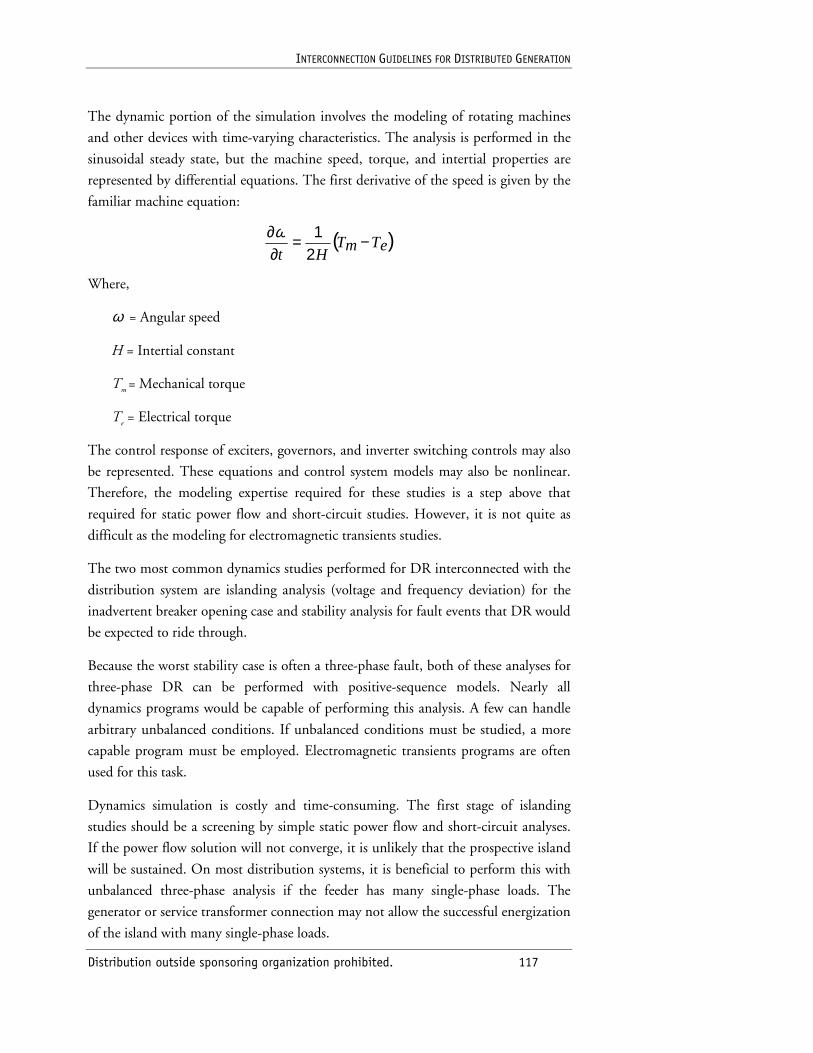
INTERCONNECTION GUIDELINES FOR DISTRIBUTED GENERATION
Distribution outside sponsoring organization prohibited. 117
The dynamic portion of the simulation involves the modeling of rotating machines
and other devices with time-varying characteristics. The analysis is performed in the
sinusoidal steady state, but the machine speed, torque, and intertial properties are
represented by differential equations. The first derivative of the speed is given by the
familiar machine equation:
( )eTmTHt
−=∂∂
21ω
Where,
ω = Angular speed
H = Intertial constant
Tm = Mechanical torque
Te = Electrical torque
The control response of exciters, governors, and inverter switching controls may also
be represented. These equations and control system models may also be nonlinear.
Therefore, the modeling expertise required for these studies is a step above that
required for static power flow and short-circuit studies. However, it is not quite as
difficult as the modeling for electromagnetic transients studies.
The two most common dynamics studies performed for DR interconnected with the
distribution system are islanding analysis (voltage and frequency deviation) for the
inadvertent breaker opening case and stability analysis for fault events that DR would
be expected to ride through.
Because the worst stability case is often a three-phase fault, both of these analyses for
three-phase DR can be performed with positive-sequence models. Nearly all
dynamics programs would be capable of performing this analysis. A few can handle
arbitrary unbalanced conditions. If unbalanced conditions must be studied, a more
capable program must be employed. Electromagnetic transients programs are often
used for this task.
Dynamics simulation is costly and time-consuming. The first stage of islanding
studies should be a screening by simple static power flow and short-circuit analyses.
If the power flow solution will not converge, it is unlikely that the prospective island
will be sustained. On most distribution systems, it is beneficial to perform this with
unbalanced three-phase analysis if the feeder has many single-phase loads. The
generator or service transformer connection may not allow the successful energization
of the island with many single-phase loads.
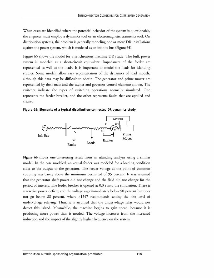
INTERCONNECTION GUIDELINES FOR DISTRIBUTED GENERATION
Distribution outside sponsoring organization prohibited. 118
When cases are identified where the potential behavior of the system is questionable,
the engineer must employ a dynamics tool or an electromagnetic transients tool. On
distribution systems, the problem is generally modeling one or more DR installations
against the power system, which is modeled as an infinite bus (Figure 65).
Figure 65 shows the model for a synchronous machine DR study. The bulk power
system is modeled as a short-circuit equivalent. Impedances of the feeder are
represented as well as the loads. It is important to model the loads for islanding
studies. Some models allow easy representation of the dynamics of load models,
although this data may be difficult to obtain. The generator and prime mover are
represented by their mass and the exciter and governor control elements shown. The
switches indicate the types of switching operations normally simulated. One
represents the feeder breaker, and the other represents faults that are applied and
cleared.
Figure 65: Elements of a typical distribution-connected DR dynamics study
Inf. BusExciter
Faults
GPrime Mover
Loads
V, I
Governor
ω, TP
Inf. BusExciter
Faults
GPrime Mover
Loads
V, I
Governor
ω, TP
Figure 66 shows one interesting result from an islanding analysis using a similar
model. In the case modeled, an actual feeder was modeled for a loading condition
close to the output of the generator. The feeder voltage at the point of common
coupling was barely above the minimum permitted of 95 percent. It was assumed
that the generator shaft power did not change and the field did not change for the
period of interest. The feeder breaker is opened at 0.3 s into the simulation. There is
a reactive power deficit, and the voltage sags immediately below 90 percent but does
not go below 88 percent, where P1547 recommends setting the first level of
undervoltage relaying. Thus, it is assumed that the undervoltage relay would not
detect this island. Meanwhile, the machine begins to gain speed, because it is
producing more power than is needed. The voltage increases from the increased
induction and the impact of the slightly higher frequency on the system.
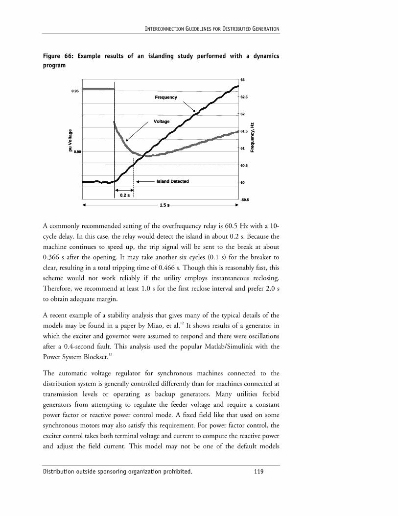
INTERCONNECTION GUIDELINES FOR DISTRIBUTED GENERATION
Distribution outside sponsoring organization prohibited. 119
Figure 66: Example results of an islanding study performed with a dynamics program
0.90
0.95
pu
Vo
ltag
e
-59.5
60
60.5
61
61.5
62
62.5
63
Fre
qu
ency
, Hz
0.2 s
Voltage
Frequency
1.5 s
Island Detected
0.90
0.95
pu
Vo
ltag
e
-59.5
60
60.5
61
61.5
62
62.5
63
Fre
qu
ency
, Hz
0.2 s
Voltage
Frequency
1.5 s
Island Detected
A commonly recommended setting of the overfrequency relay is 60.5 Hz with a 10-
cycle delay. In this case, the relay would detect the island in about 0.2 s. Because the
machine continues to speed up, the trip signal will be sent to the break at about
0.366 s after the opening. It may take another six cycles (0.1 s) for the breaker to
clear, resulting in a total tripping time of 0.466 s. Though this is reasonably fast, this
scheme would not work reliably if the utility employs instantaneous reclosing.
Therefore, we recommend at least 1.0 s for the first reclose interval and prefer 2.0 s
to obtain adequate margin.
A recent example of a stability analysis that gives many of the typical details of the
models may be found in a paper by Miao, et al.12 It shows results of a generator in
which the exciter and governor were assumed to respond and there were oscillations
after a 0.4-second fault. This analysis used the popular Matlab/Simulink with the
Power System Blockset.13
The automatic voltage regulator for synchronous machines connected to the
distribution system is generally controlled differently than for machines connected at
transmission levels or operating as backup generators. Many utilities forbid
generators from attempting to regulate the feeder voltage and require a constant
power factor or reactive power control mode. A fixed field like that used on some
synchronous motors may also satisfy this requirement. For power factor control, the
exciter control takes both terminal voltage and current to compute the reactive power
and adjust the field current. This model may not be one of the default models
INTERCONNECTION GUIDELINES FOR DISTRIBUTED GENERATION
Distribution outside sponsoring organization prohibited. 120
available to the user of a program designed for transmission-connected DR, making
the modeling process more difficult.
While interconnected, the governor control tries to maintain a particular output
power. It can get its power signal from the terminal voltage and current or the shaft
speed and torque. For many DR technologies, the power is controlled simply by
opening the throttle wide open, where it remains for short-term transient events.
Obtaining satisfactory data for accurate dynamics analysis of distribution systems can
be frustrating. One may encounter used machinery that has been recycled from other
facilities and whose original manufacturer is no longer in business. Typical values of
machine impedances and inertias may be assumed. Even with new equipment for
which the machine parameters are known, it may not be possible to obtain all the
parameters of the exciter and governor controls. One may be forced to assume some
generic control or assume that the field and power do not change for the period of
interest. The latter is sufficient for many cases where the period of interest is less than
0.5 s, although it is generally somewhat optimistic toward islanding detection. That
is, by not representing control actions that tend to bring voltage and frequency back
into specifications, simulation results might indicate that detection of an island is
more likely than it actually is.
Inverters
Inverters are commonly assumed to have no inertia and will shut off shortly after
trouble is detected. This can be represented in dynamics studies by switching off the
inverter shortly after initiation of the disturbing event. This will at least demonstrate
the behavior of the system with only rotating machines.
In practice, inverters will continue to supply the system with power if the terminal
voltages remain near normal. A variety of system conditions that can cause this.
IGBT inverter controls are often designed to inject current in phase with the voltage
to produce a particular power level. A simple model would be to assume a constant
power injection source, or a negative load (active power only), depending on the
capabilities of the computer program. If the switching control block diagram can be
obtained, it may be possible to represent some aspects of the control using existing
model templates.
If it is necessary to model precise inverter dynamic behavior, an electromagnetic
transient program should be used.
INTERCONNECTION GUIDELINES FOR DISTRIBUTED GENERATION
Distribution outside sponsoring organization prohibited. 121
Data Requirements for Dynamics Analysis
For all generators
■ MVA or kVA rating
■ Maximum power output
■ Rated power factor
■ Power factor operation range (leading/lagging limits)
■ Inertia of generator and prime mover, including gearcase, if any (typically
supplied in MW-sec)
For synchronous generators (typical values, see also Table 1)
■ Direct axis subtransient reactance, Xd" (0.17 pu)
■ Quadrature axis subtransient reactance, Xq" (0.20 pu)
■ Direct axis transient reactance, Xd’ (0.26 pu)
■ Quadrature axis transient reactance, Xq’ (0.26 pu)
■ Direct axis synchronous (nonsaturated) reactance, Xd (2.0 pu)
■ Quadrature axis synchronous reactance (nonsaturated), Xq (1.15 pu)
■ Direct axis subtransient open-circuit time constant, T’DO (0.035 s)
■ Quadrature axis subtransient open-circuit time constant, T’QO (0.020 s)
■ Direct axis transient open-circuit time constant, T’DO (5.6 s)
■ Quadrature axis transient open-circuit time constant, T’QO (5.6 s)
■ Armature constant, TA (0.16 s)
■ Armature resistance, RA (0.015 pu)
■ Stator leakage reactance, XL (0.14 pu)
■ Saturation at typically 100 percent and 120 percent terminal voltage
■ Block diagram of exciter and values for all variables and constants
INTERCONNECTION GUIDELINES FOR DISTRIBUTED GENERATION
Distribution outside sponsoring organization prohibited. 122
■ Block diagram of governor control and values for all variables and constants
For induction generators
Impedance data may be similar to that for synchronous machines or derived from the
following data, which may be more available:
■ Slip (speed) at full load.
■ Locked rotor current at 100 percent voltage.
■ Full load current.
■ Electrical torque-speed curve.
■ A block diagram of prime mover governor control and values for all variables and constants.
■ Normally, exciter data would not apply except in the case of doubly fed wound
rotor designs commonly used in wind turbines. This requires a special model.
7.4 Electromagnetic Transients
An electromagnetic transients program is the ultimate simulation tool for difficult
cases. It dispenses with the simplifications necessary for steady-state analysis in power
flow and dynamics tools and recreates the waveforms point-by-point. All of the
nonlinearities in the problem can be handled explicitly and as accurately as the
known data will allow. This additional capability comes at the expense of more
complicated problem setups and longer simulation times. The expertise required for
proper problem descriptions can also be substantially greater than for other tools,
although dynamics tools can also demand special skills.
Because of time requirements and the special nature of the dynamics tools, it is
expected that they will be used sparingly, if at all, by utility distribution engineers on
a regular basis. These tools will be most commonly applied by those performing
research projects, failure analyses, and designing DR equipment. Users would
typically be specialists in power system simulation.
Figure 67 illustrates the type of model used in electromagnetic transients simulation
for studying DR interconnections. The utility equivalent source is to the far right,
and the wye-connected generator is on the far left side of the diagram. The generator
is connected through a delta/wye-grounded transformer to the distribution system,
which is somewhat unusual. The fault block (center, bottom) applies various types of
faults to the distribution feeder. The distribution substation transformer is a three-
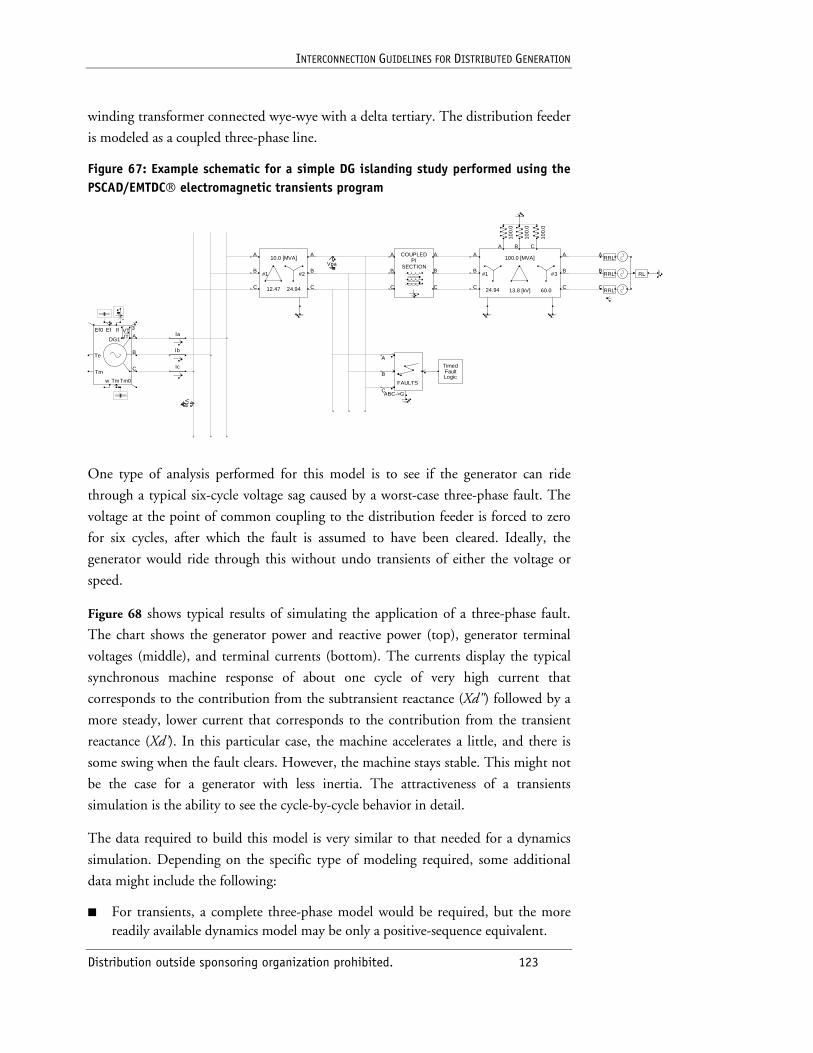
INTERCONNECTION GUIDELINES FOR DISTRIBUTED GENERATION
Distribution outside sponsoring organization prohibited. 123
winding transformer connected wye-wye with a delta tertiary. The distribution feeder
is modeled as a coupled three-phase line.
Figure 67: Example schematic for a simple DG islanding study performed using the PSCAD/EMTDC� electromagnetic transients program
A
B
C
A
B
C
A B C
100.0 [MVA]
24.94 13.8 [kV] 60.0
#1 #3
Vta
100.
0
100.
0
100.
0
Ia
Ib
Ic
A
B
C
A
B
C
10.0 [MVA]
12.47 24.94
#1 #2
COUPLED
SECTION
A
B
C
A
B
C
PIVpa
RRL
RRL
RRL
A
B
C
RL
A
B
CFAULTS
ABC->G
TimedFaultLogic
DG1
Ef0 Ef If VTIT
3
Tm0Tmw
Te
Tm
A
B
C
One type of analysis performed for this model is to see if the generator can ride
through a typical six-cycle voltage sag caused by a worst-case three-phase fault. The
voltage at the point of common coupling to the distribution feeder is forced to zero
for six cycles, after which the fault is assumed to have been cleared. Ideally, the
generator would ride through this without undo transients of either the voltage or
speed.
Figure 68 shows typical results of simulating the application of a three-phase fault.
The chart shows the generator power and reactive power (top), generator terminal
voltages (middle), and terminal currents (bottom). The currents display the typical
synchronous machine response of about one cycle of very high current that
corresponds to the contribution from the subtransient reactance (Xd") followed by a
more steady, lower current that corresponds to the contribution from the transient
reactance (Xd’). In this particular case, the machine accelerates a little, and there is
some swing when the fault clears. However, the machine stays stable. This might not
be the case for a generator with less inertia. The attractiveness of a transients
simulation is the ability to see the cycle-by-cycle behavior in detail.
The data required to build this model is very similar to that needed for a dynamics
simulation. Depending on the specific type of modeling required, some additional
data might include the following:
■ For transients, a complete three-phase model would be required, but the more readily available dynamics model may be only a positive-sequence equivalent.
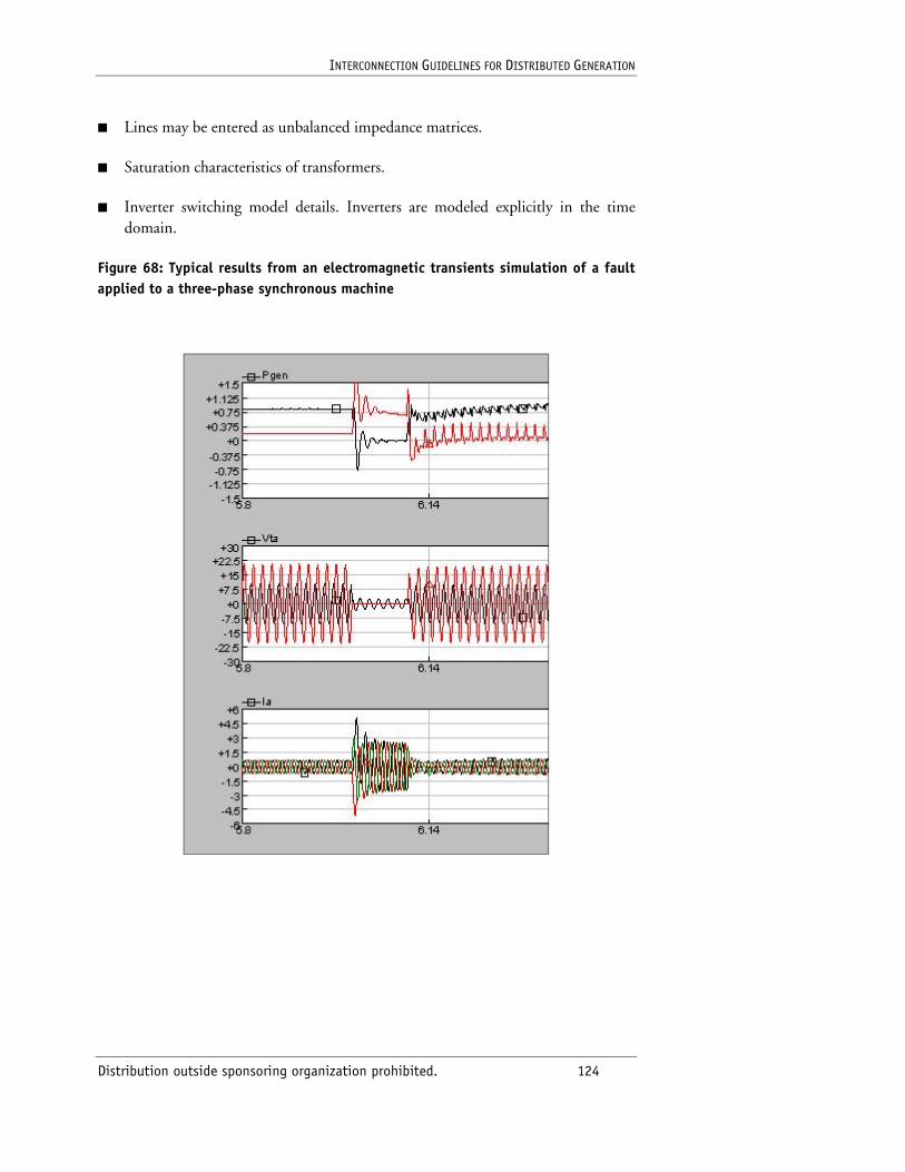
INTERCONNECTION GUIDELINES FOR DISTRIBUTED GENERATION
Distribution outside sponsoring organization prohibited. 124
■ Lines may be entered as unbalanced impedance matrices.
■ Saturation characteristics of transformers.
■ Inverter switching model details. Inverters are modeled explicitly in the time domain.
Figure 68: Typical results from an electromagnetic transients simulation of a fault applied to a three-phase synchronous machine
INTERCONNECTION GUIDELINES FOR DISTRIBUTED GENERATION
Distribution outside sponsoring organization prohibited. 125
Notes
1 IEEE Standard 519-1992, IEEE Recommended Practice and Requirements for
Harmonic Control in Electric Power Systems (1992).
2 Distribution Planning with Distributed Generation Workshop, Electrotek Concepts
Inc., Knoxville, TN, and Energy and Environmental Economics Inc., San Francisco,
CA (2000–2002).
3 C.J. Mozina, “Interconnect Protection of Dispersed Generations,” IEEE PES
Transmission and Distribution Conference, Atlanta, Georgia (November 2001).
4 Generator Protection Application Guide, Basler Electric (June 2001), from
www.basler.com and M-3520 Intertie Protection, Beckwith Electric Co. Inc., from
www.beckwithelectric.com.
5 IEC 61000-4-15, Flickermeter-Functional and Design Specifications (1997).
6 R.C. Dugan, T.E. McDermott, D.T. Rizy, and S. Steffel, “Interconnecting Single-
Phase Backup Generation to the Utility Distribution System,” IEEE PES 2001
Transmission and Distribution Conference Proceedings, Atlanta, Georgia (November
2001).
7 IEEE Standard 929-2000, Recommended Practice for Utility Interface of Photovoltaic
Systems.
8 D.R. Smith, S.R. Swanson, and J.D. Borst, “Overvoltages with Remotely Switched
Cable-Fed Grounded Wye-Wye Transformers,” IEEE Transactions on Power
Apparatus and Systems, v. PAS-94, no. 5 (September/October 1975), pp. 1843–
1853.
9 C.S. Cheng and D. Shirmohammadi, “A Three-Phase Power Flow Method for Real-
Time Distribution System Analysis,” IEEE Transactions on Power Systems, v. 10, no.
2 (May 1995), p. 671.
10 R.E. Brown, J. Pan, X. Feng, and K. Koutlev, “Siting Distributed Generation to
Defer T&D Expansion,” IEEE 2001 PES Transmission and Distribution Conference
Proceedings, Atlanta, Georgia (November 2001).
11 Electrical Distribution System Protection, Cooper Power Systems, Waukesha, WI
(1990).
INTERCONNECTION GUIDELINES FOR DISTRIBUTED GENERATION
Distribution outside sponsoring organization prohibited. 126
12 Z.Miao, M.A. Choudhry, and R. L. Klein, “Dynamic Simulation and Stability
Control of Three-Phase Distribution Systems with Distributed Generation,” IEEE
PES Winter Meeting, New York (January 2002).
13 Power System Blockset for Use with Simulink, Hydro Quebec TEQSOM
International, from www.mathworks.com.