Interactive Visualization of Multivariate Trajectory Data with Density Maps

Roeland Scheepens∗ Niels Willems† Huub van de Wetering‡ Jarke J. van Wijk§

Department of Mathematics and Computer Science, Eindhoven University of Technology, The Netherlands

Figure 1: A density map of vessel traffic in front of Rotterdam during a single day. The density map is a combination of four density fields eachcovering a quarter of the day. The following manually defined color map is used: night is dark blue, morning is bright yellow, afternoon is darkyellow, and evening is bright blue. Furthermore, the saturation of the color represents the density field contribution and the hue is given by theperiod with the highest density. To discriminate daylight patterns from nighttime, the night and evening use half the kernel radius of the otherperiods. This figure shows that the main routes are the most used during daylight, while in the night deviations from these routes occur.

ABSTRACT

We present a method to interactively explore multiple attributes intrajectory data using density maps, i.e., images that show an aggre-gate overview of massive amounts of data. So far, density mapshave mainly been used to visualize single attributes. Density mapsare created in a two-way procedure; first smoothed trajectories areaggregated in a density field, and then the density field is visualized.In our approach, the user can explore attributes along trajectoriesby calculating a density field for multiple subsets of the data. Thesedensity fields are then either combined into a new density field orfirst visualized and then combined. Using a widget, called a distri-bution map, the user can interactively define subsets in an effectiveand intuitive way, and, supported by high-end graphics hardwarethe user gets fast feedback for these computationally expensive den-sity field calculations. We show the versatility of our method withuse cases in the maritime domain: to distinguish between periodsin the temporal aggregation, to find anomalously behaving vessels,to solve ambiguities in density maps via drill down in the data, andfor risk assessments. Given the generic framework and the lack ofdomain-specific assumptions, we expect our concept to be applica-ble for trajectories in other domains as well.

Index Terms: I.3.3 [Computing Methodologies]: ComputerGraphics—Picture/Image Generation

∗e-mail: R.J.Scheepens@tue.nl†e-mail: C.M.E.Willems@tue.nl‡e-mail: H.v.d.Wetering@tue.nl§e-mail: J.J.v.Wijk@tue.nl

1 INTRODUCTION

In the analysis of moving objects we search for patterns in trajec-tory data obtained by sensors. Many movement patterns are clas-sified by Dodge et al. [6], and we can also find them in interactionbetween objects [21], clustering of trajectories [3], and aggregatedpatterns [2]. In this paper, we focus on aggregated spatial patterns,in particular those from trajectories with various attributes.

With current technology, we are able to track massive amountsof objects with other attributes than just time and position, suchas forces, object type, or object size. Additional knowledge aboutobjects can be added by attributes obtained by reasoning or usingweb sources [29]. Current state-of-the-art aggregation methods formoving objects often do not take these additional attributes intoaccount. Kernel Density Estimation (KDE) [24] is an aggregationmethod suitable for showing an overview of massive amounts ofdata and has been adapted for trajectory data, but only a few ofthese methods take attributes into account. For instance, Willemset al. [28] only encode the velocity of ships and Peters et al. [22]only encode the direction of airplanes in a density field. Since asingle density field has limited capabilities for further extensionstowards including more attributes, we focus on combining multipledensity fields [28] for subsets defined with multiple attributes.

In this paper we present a new approach for the interactive ex-ploration of density maps of trajectories with multiple attributes.Interactive exploration requires efficient and effective methods toselect subsets of interest as well as to generate density fields. As aresult, multiple density fields need to be shown simultaneously ina density map to allow the user to determine similarities and dif-ferences. With our generic model, we are able to generate a widerange of different maps, which support story telling to explain whathappened with the objects in the data set.

The paper is organized as follows: In Section 2 we discuss workrelated to density maps. Section 3 gives a model of data and den-sity of trajectories. We describe the main features of our density

Data

Density

aggregation

Visualization

Compute

density !eld1

Re

nd

erin

g

Ima

ge

com

po

stion

Density model

Density map

Density !eld

Density !eld

Density !eld

Image

Illumination

Trajectories Compute

density !eld2

Figure 2: The rendering pipeline of vessel density maps by Willems et al. [28]. From left to right, trajectories are smoothed with a large and asmall kernel resulting in two density fields. In the rendering, the large kernel density field is used for color mapping and the aggregated densityfields are used for the illumination. In the final density map, the color image and the gray-scale image with the illumination are multiplied.

maps in Section 4 and elaborate on the implementation on graphicshardware in Section 5. Section 6 shows the versatility of densitymaps with use cases. In the final section, we conclude the paperand suggestions for future work.

2 RELATED WORK

Visualization is one of the many methodologies that can be used toanalyze moving objects. In Section 2.1 we discuss a selection ofvisualizations related to moving objects. For our visualization wehave used techniques related computer graphics, such as convolu-tion as discussed in Section 2.2 and volume rendering in Section2.3. We conclude with related topics in scientific visualization andcartography in Section 2.4.

2.1 Moving Object Analysis

Additional attributes are taken into account in the analysis of mov-ing objects by Dykes et al. [7] using multiple views. A visual an-alytics tool to analyze vessel data is demonstrated by Riveiro et al.[23]. Bak et al. [4] show by means of glyphs the spatio-temporalcharacteristics of mouse trajectories in multiple areas. Hurter et al.[11] pioneer with high-end graphics hardware for interactive visu-alizations of massive amounts of airplane trajectories. All thesetrajectory visualizations have in common that they do not smooththe data, while using multiple attributes.

2.2 Convolution

KDEs are generated by convolution of the original data and smoothdata to give an overview at various levels of detail. Trajectories canalso be convolved by moving a smoothing kernel along a trajectory.To convolve trajectories, a line needs to be convolved, which hap-pens in continuous parallel coordinate plots [10] as well. Jin et al.[14] investigate methods to analytically solve the convolution equa-tions with polynomial kernels, resulting in efficient computation.Willems et al. [28] visualized vessel traffic at two levels of detailsimultaneously revealing both global patterns, such as traffic lanes,and local patterns, such as anchoring zones. Hurter et al. [12] ex-tended their own hardware-accelerated visualization with accumu-lation, where only the sample points of the trajectory are convolved,in contrast to line segments in [28] or a variant in 3D by Demsar [5].Apart from trajectories other spatio-temporal data can be convolvedas well, such as syndromic hotspots by Maciejewski et al. [18].

In our approach, we focus on specific subsets by assigning var-ious kernel radii to them. This has a similar effect as a semanticdepth of field as proposed by Kosara et al. [16], where unimpor-tant parts of an image are convolved with relatively large kernels,to disable pre-attentive vision of sharp features in these areas.

2.3 Volume Rendering

In classic volume rendering [17], an iso-surface is constructedbased on a transfer function, which is a mapping of a scalar value toa color and an opacity, to visually divide the data set in recognizablesurfaces, such as skin and bones. In our approach, we have a sim-ilar goal, since we want to divide the data in semantically differentsubsets, but instead of mapping a density value to a visualizationparameter, such as color, we take other attributes into account at theposition to be displayed. To keep the pictures interpretable by theuser, we use simple step functions, instead of continuously definedhigher-dimensional transfer functions as Kniss et al. [15] proposedto incorporate multiple attributes in volume data.

2.4 Scientific Visualization and Cartography

A convenient representation of a density field is as a regular gridof cells with values, called a raster map. Raster maps are one ofthe various techniques in multivariate scientific visualization [8].In cartography, map algebra [26] is a well-known method to math-ematically combine these raster maps to derive features. Menniset al. [19] extend map algebra to spatio-temporal data for rastermaps that change over time. Raster maps can also be combinedvisually with a grid of small glyphs as shown by Miller [20].

3 MODELS FOR TRAJECTORIES

This section gives a brief overview of the models for trajectory dataand a trajectory density field as proposed by Willems et al. [28].

3.1 Data Model

The movement of an object o is modeled by a trajectory, whichis a sequence τo of tuples αααo

i . For an object o, we abbreviate atuple as ααα i containing the following elements: a time stamp ti, aposition pi, and other derived or measured attributes, such as speedvi, type, width, and volume. The tuples are ordered by time andmost attributes can be interpolated between consecutive tuples.

For tuples ααα0 and ααα1, we reconstruct the continuous path p(t)with t ∈ [t0, t1] using the displacement x(t), which is derived fromthe measured positions pi, time stamps ti, and speed vi:

x(t) = 12 a(t− t0)

2 + v(t− t0)

with a = v1−v0

t1−t0and v = x(t0) =

||p1−p0||t1−t0

− v1−v0

2 , (1)

p(t) = p0 + x(t) p1−p0

||p1−p0||. (2)

By taking the speed measures into account as well, we obtain amore accurate approximation of the path of the actual movementfrom the sensor data. With this movement model we are ableto compute an accurate density field of trajectories, by moving asmoothing kernel along the actual path of the movement.

Trajectories

Filter1

.

.

.

Trajectories

Compute

density !eld1

r1,w1,c1

Filter2

FilterN

Compute

density !eld2

Compute

density !eldN

Rendering

ImageN

Density map

Image2

Image1

Image

composition

Data

Density model

Visualization

Density

aggregation

.

.

.

.

.

.

Illumination

r2,w2,c2

rN,wN,cN

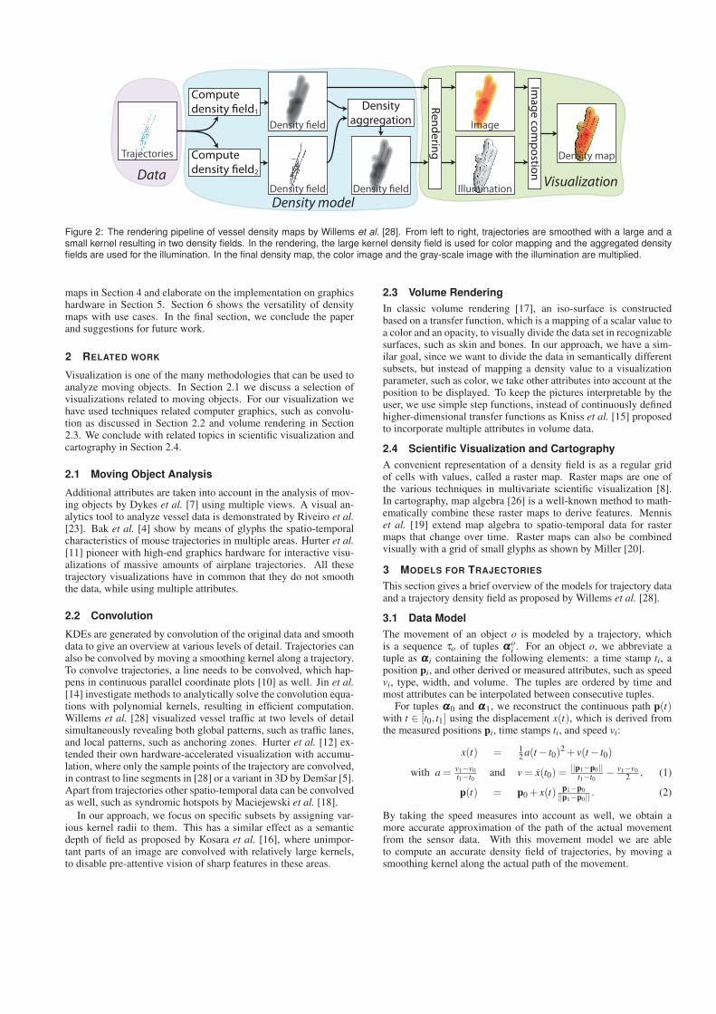
Figure 3: The architecture of our framework to generate density maps. From left to right, the trajectory data is split with various filters resulting ina number of subsets for which we compute a density field with the given weight wi and kernel radius ri. From here there are two routes. We mayaggregate the density fields in a single density field via the solid lines. Then the single density field is rendered to an image with a color map ci

and visualized together with its illumination in a density map. The other route, also via the dashed lines, first renders the density fields using acolor map ci and then composes them and applies the illumination of the aggregate density field resulting in a density map.

3.2 Density Field

In [28] trajectories are smoothed using a radially symmetric kernelfunction kr with radius r to obtain a density field with both local andglobal movement features. A continuous density field is a functionC : R2→ R, defined in [28] for a single object o with path p(t) as

Co(q) =1

T

∫ T

0kr(q−p(t))dt. (3)

Co(q) is the contribution of object o to the density in point q. Itis normalized in time to enable comparison of density fields withvarying durations. The density field C(q) of a set of trajectories isthe summation of the density fields Co(q) of all objects. We obtaina (discrete) density field D(Q) on a raster of cells by sampling C inthe center of each cell Q and multiplying by a weight w.

Figure 2 shows how density fields have been visualized as socalled vessel density maps [28]. These maps show variationsin speed as different density contributions highlighting significantmaritime areas, such as groups of high contributions for anchor-ing zones where vessels wait to enter a harbor. However, in thesemaps only a single attribute is visible. For instance, with vesseldensity maps we can not see the variations of area usage over time.Since trajectories are essentially multivariate data, the generaliza-tion of vessel density maps introduced in this paper can take moreattributes into account.

4 DENSITY MAPS

We present a framework to enhance the vessel density fields as de-scribed in the previous section with additional attributes. Figure3 shows an overview of the new architecture for density maps, inwhich the architecture for creating vessel density maps recurs. Themain principle we apply is that the data is filtered resulting in vari-ous subsets, which are aggregated into a single representation in ei-ther the density model or the visualization phase. In the remainderof this section we discuss the various aggregations in more detail.Examples of how these features can be used in real-world scenariosare shown in Section 6.

4.1 Subsets and Parameters

A density field as defined in Section 3.2 is computed based on asubset of the data defined by a filter. Typically, a filter selects alldata elements where the value of a specified attribute is within a

given range. For example, filtering on the time attribute may resultin a subset representing all objects in the night. In Section 4.5 weexplain techniques for creating filters using multiple attributes.

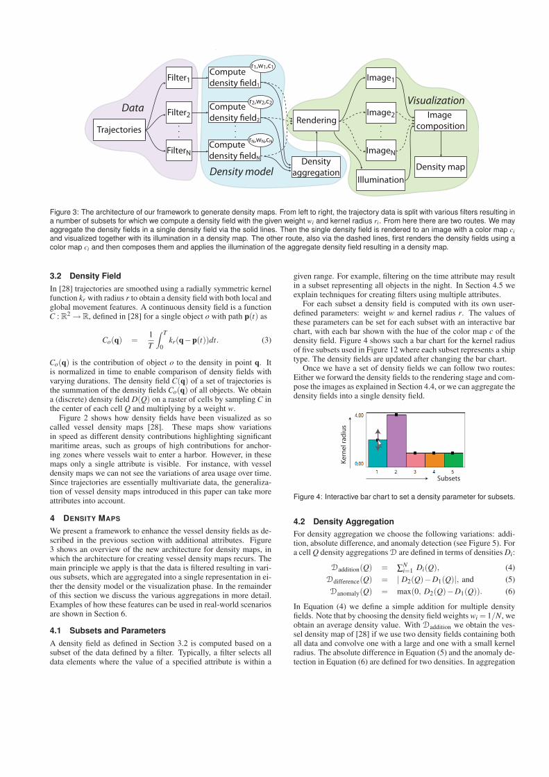
For each subset a density field is computed with its own user-defined parameters: weight w and kernel radius r. The values ofthese parameters can be set for each subset with an interactive barchart, with each bar shown with the hue of the color map c of thedensity field. Figure 4 shows such a bar chart for the kernel radiusof five subsets used in Figure 12 where each subset represents a shiptype. The density fields are updated after changing the bar chart.

Once we have a set of density fields we can follow two routes:Either we forward the density fields to the rendering stage and com-pose the images as explained in Section 4.4, or we can aggregate thedensity fields into a single density field.

Subsets

Ke

rne

l ra

diu

s

Figure 4: Interactive bar chart to set a density parameter for subsets.

4.2 Density Aggregation

For density aggregation we choose the following variations: addi-tion, absolute difference, and anomaly detection (see Figure 5). Fora cell Q density aggregations D are defined in terms of densities Di:

Daddition(Q) = ∑Ni=1 Di(Q), (4)

Ddifference(Q) = | D2(Q)−D1(Q)|, and (5)

Danomaly(Q) = max(0, D2(Q)−D1(Q)). (6)

In Equation (4) we define a simple addition for multiple densityfields. Note that by choosing the density field weights wi = 1/N, weobtain an average density value. With Daddition we obtain the ves-sel density map of [28] if we use two density fields containing bothall data and convolve one with a large and one with a small kernelradius. The absolute difference in Equation (5) and the anomaly de-tection in Equation (6) are defined for two densities. In aggregation

Ddifference, we simply search for a symmetrical difference betweenthe two density fields. The aggregation Danomaly is typically usedto find deviations of a sparse density field D2 containing instancesof behavior with respect to a dense density field D1 representingnormal movements. In Figure 5 the gray trajectory is only gray, oris anomalous, at the places where the other trajectory is not located.Section 6.2 shows anomalies with real-world data.

Figure 5: Density aggregation: (A) Weighted addition, (B) absolutedifference, and (C) anomaly detection.

4.3 Rendering

In the visualization part of the architecture in Figure 3 the densityfields are rendered to images by mapping density values to colorsvia a color map c. For a small number of density fields a singlehue color map is used for each density field. The user is supportedby a preset of clearly distinguishable hues to obtain a perceptuallybalanced map, as used in Figure 12. The preset is a pastel rainbowcolor map generated with PaletteView [27] and sampled at equal in-tervals for a given number of colors. The chosen color is associatedto the highest density value of the field, and a complete color map iscreated by interpolating the saturation towards white, see the lowerright corner of Figure 11.

If only one density field is visualized a multi-hue color map canbe used, as hue is not needed to distinguish between density fields.We can choose, for instance, to use a yellow-to-red color map withmore contrast between density levels, as used in Figure 9 and 11A.

4.4 Image Composition

Not only density fields but also the color mapped images of densityfields can be aggregated. To obtain a density map, we aggregate thecolor mapped images with an operation called image compositionand, finally, apply Phong shading on a height field given by thedensity aggregation field (see Figure 3).

We distinguish five types of image compositions: single-fieldIsingle, aggregate-field Iaggregate, opacity-blend Iopacity, max-blend

Figure 6: Image composition: (A) Single-field, (B) multi-field, (C)opacity-blend, (D) max-blend, and (E) block.

Imax, and block Iblock (see Figure 6). The output of Isingle is simplyone of the color mapped density fields and for Iaggregate it is thecolor mapped aggregated density field obtained by D. Since thesetwo image compositions have a single density field as input they canuse a multi-hue color map. In the vessel density shown in Figure11A Isingle is used, in Figure 9 Iaggregate is used.

The Iopacity composition is a weighted sum of the colors of therendered density fields in RGB-space with the opacity as weight.With Imax we show the color of the density field with the highestvalue, as used in Figure 1. From the latter two image compositionsit is hard to see which colors are used in a certain neighborhood,therefore we introduce Iblock. In this image composition, a new im-age is created covering the same area as the input images, but witha much lower resolution to avoid dithering effects. The color ofthe pixels in this new image are set as follows: If a pixel overlapswith one or more density values larger than zero, one of these den-sity fields is randomly chosen and the corresponding color is used.Hagh et al. [9] have evaluated this composition, called color weav-ing, and show that it is more effective than color blending (Iopacity)for two to four colors, while for upto six colors the error rates sig-nificantly increase. In Section 6.3, Iblock is used to reveal variousship type in a neighborhood.

4.5 Multivariate Filters

So far, filters for single attributes have been considered. We canexpand the usability of our method greatly by defining interactivefilters based on multiple attributes. To this end, we have developedan interactive widget, called a Distribution Map (DM), as shown inFigure 7 with various pairs of attributes used in vessel tracking.

Time

Ve

sse

l Are

a

Velocity

Ve

sse

l Ty

pe

Velocity

Ve

sse

l Are

a

D EC

Time

Ve

loci

ty

Time

Ve

sse

l Ty

pe

A B

Figure 7: Distribution maps from pairs of vessel attributes.

A DM consists of a 2D-plane with two axes corresponding to twochosen attributes and shows in gray-scale the distribution of the val-ues of these attributes as they appear in the trajectories. Guided bythis distribution, the user, while defining a filter, selects combina-tions of attribute intervals by drawing a set of rectangles, coloredwith the same hue as the color map c for rendering the density field.For example the pink rectangles in Figure 7A represent medium-speed moving vessels in the morning together with fast movingvessels in the evening. Adaptations of the rectangles result in anupdate of the density field of the corresponding subset.

The distributions are generated by drawing, with additive blend-ing, bright gray polylines as trajectories for the two attributes givenon the axes. With this technique we mimic counting how long anattribute pair occurs in the trajectories.

Construct

OBB Rasterize

Compute

density

Grid in Geographic Space

Blend to

frame bu!er

Geometry shader Fragment shaderRasterizer

Render Output Unit

p1

p0

v3

v1

v2

v4

A B C DKernel radius

Frame bu!er

Video Memory

Figure 8: The pipeline for computing density fields on a GPU: (A) The trajectory segment p0p1 given in geographic coordinates. (B) The segmentmapped to map coordinates using the cylindrical equal-area projection and its OBB v1v2v3v4 at distance r. (C) The fragments inside OBB. (D)The density field computed for each fragment in OBB. This density field is then added to already computed densities of other segments.

5 IMPLEMENTATION

In this section we give a method for parallel computation of densityfields on the GPU based on the non-parallel version in [28]. As inthat algorithm we assume that the trajectory points are given in ge-ographic coordinates and a cylindrical equal-area map-projectionG [25] is used to transform these in map coordinates. Given thedensity fields the visualization of the final density map is straight-forward, also realized on the GPU, and omitted here.

5.1 Parallelization

A method for parallelization of density field computations eitherhas an image-space or an object-space approach. In an image-spaceapproach the parallelization is done over computations per pixel,where in an object-space approach it is done over computations perobject. Here we chose an object-space approach where we sim-ply traverse the objects, in this case the trajectory segments. Addi-tional advantages are that adding and removing trajectory segmentsis trivial and that the regular graphics pipeline elements, such as therasterizer and the render output unit, can be used without explicitsynchronization to obtain high throughput.

Algorithm 1 ParallelComputeDensityField()

CopyTrajectoriesToVideoMemory()D← 0H,B {D becomes zero matrix}for o ∈ Objects do

for tuples ααα i and ααα i+1 in trajectory τo do in parallelp0← po(ti);p1← po(ti+1)OBB← oriented bounding box at distance K to p0p1

for (u,v) ∈ OBB do in parallel{Get geographical coordinate of the cell center}q← G−1(u,v){Assign density based on Equation (3) in Section 3.2}D(u,v)← D(u,v)+Cp0p1

(q)return D;

Our approach is given in pseudo code in Algorithm 1 and il-lustrated in Figure 8. We first construct a texture according to thesubdivision of our geographic space into uniform cells with equalarea. For each vessel o we render its trajectories to this texture thatultimately represents the density field. For each trajectory we han-dle all line segments between two consecutive tuples ααα i and ααα i+1.Line segments are processed in parallel by geometry shaders thatconstruct, given a line segment p0p1, an oriented bounding box(OBB) for the points at most distance r, the kernel radius, from therhumb line p0p1 [1] and return four vertices defining an OBB (seeFigure 8B). Using the rasterizer the OBB is then subdivided intofragments (see Figure 8C), representing the cells to whose densitythe object o contributes. For each fragment (u,v) a fragment shaderis run that computes the geographical coordinates q of the frag-ment (see Figure 8D) using the inverse of the cylindrical equal-area

map-projection G. Finally, the density contribution Cp0p1(q) is ad-

ditively blended into density field D by the render output unit.

Some issues are not handled in the pseudo code of Algorithm 1.First, for reasons of accuracy almost stationary objects are handleddifferent in the sense that their density is computed by drawing atexture mapped fat point with radius r. Second, the standard for-mula for computing the great circle distance, which is inaccuratefor points at small distances, is replaced by an approximation thatis stable for such points. Third, numerical integration of Equation(3) uses Simpson’s rule. And finally, kernel evaluation is a texturelook up, which allows to us to use arbitrary finite-support kernels.

5.2 Performance

The pictures and performance tests in this paper have been gen-erated on an Intel Core i7 CPU at 2.8 GHz with 6 GB of RAMmemory and an NVidia GeForce GTX 285 with 1 GB of videomemory. The computation time of visualizing a single density fielddepends on the size of the density field, the kernel radius, the num-ber of steps in the integral approximations, and the size of the dataset. For a typical data set, containing data from a single day inthe North Sea with 1390 objects and 306,521 data points, a densityfield of 1250x1020 cells, representing an area of 125 km by 102km, is computed and displayed on a screen of 900x900 pixels in,on average, 0.77 seconds for a kernel radius of 2 km. This does notgive full interactive rate, but this can be accomplished by diminish-ing the accuracy of the density map during interaction. There areseveral ways to do so. First of all reducing in the above examplethe density map to 125x102 cells and using Catmull-Rom spline in-terpolation for intermediate values reduces the computation time to0.13 seconds. The cell size is then still half the kernel radius and theoverall appearance of the image remains intact. Alternatively, thenumber of numerical integration steps can be reduced from the de-fault 10 steps to 5 steps to gain up to a factor of two in performancewhile still obtaining acceptable results.

The interactivity could suffer when computing multiple densityfields for a single density map. However, in practice, this is notproblematic. If for the density map the data has been split in severalsubsets, one for each density field, the total computation time is ap-proximately the computation time of a density field using the com-plete data set. If the density map requires multiple density fieldsusing the full data set, the interaction is mostly such that only onedensity field needs recomputation and in this case only the initialcomputation of the density map is relatively slow.

6 MARITIME USE CASES

The density map framework is intended for expert users, who ex-plore distributions of attributes defined along trajectories. In theexploration, the user mainly interacts with the distribution maps,though the framework is extensive in fine tuning for optimizing de-tails in the density maps. One of the possible outcomes of the ex-ploration is a density map, which can be used as a static overlay

in addition to the regular operational maps containing live trafficfor supporting monitoring tasks. To show the expressiveness of ourframework, we have defined various use cases towards open prob-lems in the analysis of moving objects with a density approach. Theuse cases are taken from the maritime domain and concern trajec-tory data from vessels.

Professional vessels with a gross tonnage of three hundred tonsand up are obliged to broadcast their current status using the Auto-matic Identification System (AIS) [13]. The trajectory data consistsof many attributes, such as time, location, ship type, dimensions,destination, and so forth. AIS is used for safety and security byeither captains sailing on board of a ship, or by surveillance oper-ators guarding coastal areas. Historical AIS data can be used forplanning of the spatial usage of coastal areas, for instance by val-idating whether or not all ships have followed the rules. The dataset contains both route-bounded vessels (e.g., tankers, cargo ships)and non-route-bounded vessels (e.g., pleasure craft, tugs), hintingthat our method works for both constrained trajectories (e.g., cars,trains) and unconstrained trajectories (e.g., animals, pedestrians).

6.1 Temporal Aggregation

In a vessel density map [28], the order in which movements takeplace is lost, since all trajectories are convolved with the samesmoothing kernel. With the new density maps, we can vary the ker-nel radius and kernel weight over time. Figure 9 shows a single dayof vessel traffic in front of Rotterdam harbor with four subsets ofsix hours. During the day, the kernel radius is decreasing, while theweights are increasing, and by using density aggregation Daddition

various moments in time are distinguishable. The resulting densitymap consist of a rendering in both color and illumination of a singleaggregated density field using Iaggregate image composition.

We

igh

tR

ad

ius

Figure 9: An aggregation of four density maps each covering sixhours of a day using addition as density aggregation.

In Figure 9 we see that the subset in the evening, shown withsmall and dark trajectories are highlighted, while the others serveas a context. Noticeable movement patterns in these trajectories inthe evening that were not visible before are encircled. In the circleswe clearly distinguish relatively high density along narrow tracksindicating slow moving night ships. Notice that we can also showvariations over time using image composition Imax as displayed inFigure 1.

6.2 Anomaly Detection

A density field of a reasonable amount of trajectories represents thenautical history in an area, indicating, for instance, which move-ments are usual. By comparing other trajectories with this densityfield, we can determine abnormal behavior in areas where the den-sity field values are low. Density maps can be used to show theseanomalously behaving vessels. Figure 10 shows the result of thedensity aggregation Danomaly of two density fields: one with sixdays of data between Amsterdam and Scheveningen and a densityfield with the traffic from the last two hours, which can be animatedby varying the current time. For the latter one, the kernel radiusis decreasing backwards in time, i.e., the head is the most currentposition. The resulting density field is shown with Isingle imagecomposition and displays potential anomalies in color from white(none) and green (low) to red (high) in the context of all data shownin the shading. This example shows how density based anomaly de-tection can be used in a real-time system.

Figure 10: A vessel sailing between Amsterdam and Scheveningenis marked as anomalous, since normally no vessels sail in this area.

6.3 Stopping Areas

A vessel density map [28] highlights anchoring zones as groupsof dark dot-like parts of trajectories, as shown in the rectangles inFigure 11A. However, similar dark features popup for other slowmovements, which are not in anchoring zones. In this use case, wetry to find explanations for what happens in these areas.

First, we isolate the areas with slow movements by defining twosubsets using the DM shown in Figure 11B; a red subset for station-ary vessels and a blue one for moving vessels. Using image compo-sition Imax we show the colors assigned to the subsets in the densitymap of Figure 11C. The official anchoring zones are marked withan anchor. Area number 7 is Rotterdam harbor. The other areaswith slow movement need additional inspection.

The type of a vessel and the way it moves often explains whathappens. Therefore, we change the time axis of the DM to velocityand change the velocity axis to vessel type (see Figure 11D) anddefine six subsets with slow moving vessels of different types. Thecolors of the subsets in the DM correspond with the legend on thebottom right of Figure 11. To find the various subsets available inthese small areas we use Iblock for image composition. In Figure11E we see a cargo ship and a nearby tanker. When decreasing the

Figure 11: Classifying behavior of slow moving vessels in front of Rotterdam harbor during one week. In (A) a vessel density map [28] is shownand in (C) slow moving areas are isolated using the DM in (B) and anchor zones are marked with an anchor. After defining different types of slowmoving vessels with the DM in (D) we can figure out what happened in the zoomed in areas (E...I), which correspond with the numbers in (C).

kernel radius black squares indicating oil platforms become visible(see inset) and actually explain the slow moving vessels. The sur-roundings of the harbor of Scheveningen with its popular beach areshown in 11F. Some typical vessels close to the coast are visiblevia a manually defined color map: fishing vessels (yellow), plea-sure craft (green), special craft, e.g., a rescue vessel, in red, andothers, often small crafts, in pink. Noticeable in this area is a cargoship (blue) relatively close to the beach; this is suspicious as suchships are not expected close to the coast. In Figure 11G, there aretwo hotspots with small vessel types; the one on the right is theharbor of the city Hellevoetsluis, while the left one is near the Har-ingvlietdam. The existence of a lock explains the concentration ofwaiting ships on the bottom left-hand side of the Haringvlietdamand also explains why only small vessels sail in this neighborhood.By clicking on vessels we find in Figure 11H that the special craftsare a dredger at work (left) and a law enforcement vessel (right). Inthe course of its duty the latter stops multiple times. Finally, Figure11I shows a potential threat since a fisher stops in a sea lane.

6.4 Risk Assessment

Some vessels are more dangerous than others. In this use case, wecreate a density map showing the possible risks of various vesseltypes. In the DM we put the vessel type and the area on the axesand define the following subsets, with ’large’ being a larger areathan 9000 m2 and ’small’ the rest: Large cargo vessels (blue), largetankers (purple), small passenger ships (pink), small high speedcraft (orange) and other type of small ships (green). The color mapis given by the color map preset mentioned in Section 4.4. Thecolor mapped densities are composed with Imax to show the mostdangerous types in an certain area. To illustrate possible risks ofdangerous vessels, we have identified three classes of danger andwe have assigned a large kernel with high weight for more dan-gerous vessel types. In this risk density map we can see that theshoreline is not put in danger, and that dangerous tankers take theleft route, while less dangerous cargo vessels take the route closerto the shore.

Figure 12: A risk map with various vessel types: large cargo vessels(blue), large tankers (purple), small passenger ships (pink), smallhigh speed craft (orange), and other type of small ships (green).

7 CONCLUSIONS AND FUTURE WORK

We have presented a method to explore multivariate trajectorieswith density maps. To support massive real-world trajectory datasets, we have significantly improved the density field computationtime with respect to previous implementations by means of high-end graphics hardware. As a result, we are able to combine multipledensity fields quickly, which allows us to enrich density maps. Thecombination of density fields takes place in either density aggrega-tion or the combination of images of density fields, which can beinteractively defined by the user. Density aggregation is typicallyuseful for quantitative analysis, while image composition enables tomake a distinction between subsets. The set of aggregations tendsto be fairly complete, though the framework can be extended easilywith new aggregations. We have applied our method to vessel tra-jectories allowing us to reveal what takes place when, find anoma-lously behaving vessels, drill down on attributes to solve ambigui-ties in density fields, and conduct risk assessments.

In future research, we will further investigate the parameters inour method, the interaction to set them, and possibilities for newvisual cues to render these parameters. A user study should answerhow effective density maps are for analysis tasks. The frameworkmay be extended with a multi-pass technique that takes a densityfield as a parameter for another density field. For instance, we canvary the kernel radius based on another density field. For vessels,this could lead, for instance, to more features in busy harbors, ifthe kernel radius is decreased for higher densities. Furthermore, thedirection is an important feature of trajectory data, which has notbeen addressed yet in density maps in an appropriate way. Finally,we are interested if the method can support analysis of moving ob-jects in other domains, by exploring different data sets.

ACKNOWLEDGEMENTS

We thank the reviewers and Hans Hiemstra for their feedback. Thiswork has been carried out as a part of the Poseidon project at ThalesNederland under the responsibilities of the Embedded Systems In-stitute (ESI). This project is partially supported by the Dutch Min-istry of Economic Affairs under the BSIK program.

REFERENCES

[1] J. Alexander. Loxodromes: A rhumb way to go. Mathematics maga-

zine, 77(5):349–356, Dec. 2004.

[2] G. Andrienko and N. Andrienko. Spatio-temporal aggregation for vi-

sual analysis of movements. IEEE VAST, pages 51–58, October 2008.

[3] G. Andrienko et al. Interactive visual clustering of large collections

of trajectories. IEEE VAST, pages 3–10, October 2009.

[4] P. Bak et al. Spatiotemporal analysis of sensor logs using growth ring

maps. IEEE TVCG, 15(6):913–920, 2009.

[5] U. Demsar and K. Virrantaus. Space-time density of trajectories:

Exploring spatio-temporal patterns in movement data. International

Journal of Geographical Information Science, 24(10):1527–1542,

October 2010.

[6] S. Dodge, R. Weibel, and A.-K. Lautenschutz. Towards a taxonomy

of movement patterns. Information Visualization, 7(3–4):240 – 252.

[7] J. A. Dykes and D. M. Mountain. Seeking structure in records of

spatio-temporal behaviour. Computational Statistics & Data Analysis,

43(4):581–603, 2003. Data Visualization.

[8] R. Fuchs and H. Hauser. Visualization of multi-variate scientific data.

Computer Graphics Forum, 28(6):1670–1690, 2009.

[9] H. Hagh-Shenas, S. Kim, V. Interrante, and C. Healey. Weaving versus

blending. IEEE TVCG, 13:1270–1277, 2007.

[10] J. Heinrich and D. Weiskopf. Continuous parallel coordinates. IEEE

TVCG, 15:1531–1538, 2009.

[11] C. Hurter, B. Tissoires, and S. Conversy. FromDaDy: Spreading

aircraft trajectories across views to support iterative queries. IEEE

TVCG, 15(6):1017–1024, 2009.

[12] C. Hurter, B. Tissoires, and S. Conversy. Accumulation as a tool for ef-

ficient visualization of geographical and temporal data. AGILE Work-

shop Geospatial Visual Analytics: Focus on Time, May 2010.

[13] ITU. Technical characteristics for an automatic identification system

using time division multiple access in the VHF maritime mobile band.

Recommendation ITU-R M.1371-1, 2001.

[14] X. Jin and C.-L. Tai. Analytical methods for polynomial weighted

convolution surfaces with various kernels. Computers & Graphics,

26(3):437–447, June 2002.

[15] J. Kniss et al. Multidimensional transfer functions for interactive vol-

ume rendering. IEEE TVCG, 8:270–285, 2002.

[16] R. Kosara, S. Miksch, and H. Hauser. Focus+context taken literally.

IEEE CG&A, 22:22–29, 2002.

[17] M. Levoy. Display of surfaces from volume data. Computer Graphics

and Applications, 8(3):29–37, May 1988.

[18] R. Maciejewski et al. A visual analytics approach to understanding

spatiotemporal hotspots. IEEE TVCG, 99(RP):205–220, 2009.

[19] J. Mennis, R. Viger, and C. D. Tomlin. Cubic map algebra functions

for spatio-temporal analysis. Cartography and GIS, 32:17–32, 2005.

[20] J. R. Miller. Attribute blocks: Visualizing multiple continuously de-

fined attributes. IEEE CG&A, 27:57–69, 2007.

[21] D. Orellana et al. Uncovering interaction patterns in mobile outdoor

gaming. International Conference on Advanced Geographic Informa-

tion Systems & Web Services, pages 177–182, 2009.

[22] S. Peters and J. M. Krisp. Density calculation for moving points. AG-

ILE Int. Conference on Geographic Information Science, 2010.

[23] M. Riveiro, G. Falkman, and T. Ziemke. Visual analytics for the de-

tection of anomalous maritime behavior. In International Conference

Information Visualization, pages 273–279, 2008.

[24] B. W. Silverman. Density Estimation for Statistics and Data Analy-

sis. Number 26 in Monographs on Statistics and Applied Probability.

Chapman & Hall, 1992.

[25] J. P. Snyder. Flattening the Earth: Two Thousand Years of Map Pro-

jections. University of Chicago Press, 1993.

[26] C. D. Tomlin and J. K. Berry. A mathematical structure for carto-

graphic modeling in environmental analysis. Symposium of the Amer-

ican Congress on Surveying and Mapping, pages 269–283, 1979.

[27] M. Wijffelaars, R. Vliegen, J. J. van Wijk, and E.-J. van der Lin-

den. Generating color palettes using intuitive parameters. Computer

Graphics Forum, 27(8):743–750, May 2008.

[28] N. Willems, H. van de Wetering, and J. J. van Wijk. Visualization of

vessel movements. Computer Graphics Forum, 28(3):959–966, 2009.

[29] N. Willems, W. R. van Hage, G. de Vries, J. H. Janssens, and

V. Malaise. An integrated approach for visual analysis of a multi-

source moving objects knowledge base. International Journal of Ge-

ographical Information Science, 24(10):1543–1558, October 2010.