Interactive Multiresolution Mesh Editing

Denis Zorin∗

CaltechPeter Schroder†

CaltechWim Sweldens‡

Bell Laboratories

AbstractWe describe a multiresolution representation for meshes based onsubdivision, which is a natural extension of the existing patch-basedsurface representations. Combining subdivision and the smooth-ing algorithms of Taubin [26] allows us to construct a set of algo-rithms for interactive multiresolution editing of complex hierarchi-cal meshes of arbitrary topology. The simplicity of the underly-ing algorithms for refinement and coarsification enables us to makethem local and adaptive, thereby considerably improving their effi-ciency. We have built a scalable interactive multiresolution editingsystem based on such algorithms.

1 IntroductionApplications such as special effects and animation require creationand manipulation of complex geometric models of arbitrary topol-ogy. Like real world geometry, these models often carry detail atmany scales (cf. Fig. 1). The model might be constructed fromscratch (ab initio design) in an interactive modeling environment orbe scanned-in either by hand or with automatic digitizing methods.The latter is a common source of data particularly in the entertain-ment industry. When using laser range scanners, for example, indi-vidual models are often composed of high resolution meshes withhundreds of thousands to millions of triangles.

Manipulating such fine meshes can be difficult, especially whenthey are to be edited or animated. Interactivity, which is crucial inthese cases, is challenging to achieve. Even without accounting forany computation on the mesh itself, available rendering resourcesalone, may not be able to cope with the sheer size of the data. Pos-sible approaches include mesh optimization [15, 13] to reduce thesize of the meshes.

Aside from considerations of economy, the choice of represen-tation is also guided by the need for multiresolution editing se-mantics. The representation of the mesh needs to provide con-trol at a large scale, so that one can change the mesh in a broad,smooth manner, for example. Additionally designers will typi-cally also want control over the minute features of the model (cf.Fig. 1). Smoother approximations can be built through the use ofpatches [14], though at the cost of loosing the high frequency de-tails. Such detail can be reintroduced by combining patches withdisplacement maps [17]. However, this is difficult to manage in the

∗dzorin@gg.caltech.edu†ps@cs.caltech.edu‡wim@bell-labs.com

arbitrary topology setting and across a continuous range of scalesand hardware resources.

Figure 1: Before the Armadillo started working out he was flabby,complete with a double chin. Now he exercises regularly. The orig-inal is on the right (courtesy Venkat Krischnamurthy). The editedversion on the left illustrates large scale edits, such as his belly, andsmaller scale edits such as his double chin; all edits were performedat about 5 frames per second on an Indigo R10000 Solid Impact.

For reasons of efficiency the algorithms should be highly adap-tive and dynamically adjust to available resources. Our goal is tohave a single, simple, uniform representation with scalable algo-rithms. The system should be capable of delivering multiple framesper second update rates even on small workstations taking advan-tage of lower resolution representations.

In this paper we present a system which possesses these proper-ties

• Multiresolution control: Both broad and general handles, aswell as small knobs to tweak minute detail are available.

• Speed/fidelity tradeoff: All algorithms dynamically adapt toavailable resources to maintain interactivity.

• Simplicity/uniformity: A single primitive, triangular mesh, isused to represent the surface across all levels of resolution.

Our system is inspired by a number of earlier approaches. Wemention multiresolution editing [11, 9, 12], arbitrary topology sub-division [6, 2, 19, 7, 28, 16], wavelet representations [21, 24, 8, 3],and mesh simplification [13, 17]. Independently an approach simi-lar to ours was developed by Pulli and Lounsbery [23].

It should be noted that our methods rely on the finest level meshhaving subdivision connectivity. This requires a remeshing step be-fore external high resolution geometry can be imported into the ed-itor. Eck et al. [8] have described a possible approach to remeshingarbitrary finest level input meshes fully automatically. A methodthat relies on a user’s expertise was developed by Krishnamurthyand Levoy [17].

1.1 Earlier Editing ApproachesH-splines were presented in pioneering work on hierarchicalediting by Forsey and Bartels [11]. Briefly, H-splines are obtainedby adding finer resolution B-splines onto an existing coarser resolu-tion B-spline patch relative to the coordinate frame induced by the

coarser patch. Repeating this process, one can build very compli-cated shapes which are entirely parameterized over the unit square.Forsey and Bartels observed that the hierarchy induced coordinateframe for the offsets is essential to achieve correct editing seman-tics.

H-splines provide a uniform framework for representing both thecoarse and fine level details. Note however, that as more detailis added to such a model the internal control mesh data structuresmore and more resemble a fine polyhedral mesh.

While their original implementation allowed only for regulartopologies their approach could be extended to the general settingby using surface splines or one of the spline derived general topol-ogy subdivision schemes [18]. However, these schemes have notyet been made to work adaptively.

Forsey and Bartels’ original work focused on the ab initio de-sign setting. There the user’s help is enlisted in defining what ismeant by different levels of resolution. The user decides where toadd detail and manipulates the corresponding controls. This waythe levels of the hierarchy are hand built by a human user and therepresentation of the final object is a function of its editing history.

To edit an a priori given model it is crucial to have a general pro-cedure to define coarser levels and compute details between levels.We refer to this as the analysis algorithm. An H-spline analysis al-gorithm based on weighted least squares was introduced [10], butis too expensive to run interactively. Note that even in an ab initiodesign setting online analysis is needed, since after a long sequenceof editing steps the H-spline is likely to be overly refined and needsto be consolidated.

Wavelets provide a framework in which to rigorously de-fine multiresolution approximations and fast analysis algorithms.Finkelstein and Salesin [9], for example, used B-spline waveletsto describe multiresolution editing of curves. As in H-splines, pa-rameterization of details with respect to a coordinate frame inducedby the coarser level approximation is required to get correct edit-ing semantics. Gortler and Cohen [12], pointed out that waveletrepresentations of detail tend to behave in undesirable ways duringediting and returned to a pure B-spline representation as used inH-splines.

Carrying these constructions over into the arbitrary topology sur-face framework is not straightforward. In the work by Lounsbery etal. [21] the connection between wavelets and subdivision was usedto define the different levels of resolution. The original construc-tions were limited to piecewise linear subdivision, but smootherconstructions are possible [24, 28].

An approach to surface modeling based on variational methodswas proposed by Welch and Witkin [27]. An attractive character-istic of their method is flexibility in the choice of control points.However, they use a global optimization procedure to compute thesurface which is not suitable for interactive manipulation of com-plex surfaces.

Before we proceed to a more detailed discussion of editing wefirst discuss different surface representations to motivate our choiceof synthesis (refinement) algorithm.

1.2 Surface RepresentationsThere are many possible choices for surface representations.Among the most popular are polynomial patches and polygons.

Patches are a powerful primitive for the construction of coarsegrain, smooth models using a small number of control parameters.Combined with hardware support relatively fast implementationsare possible. However, when building complex models with manypatches the preservation of smoothness across patch boundaries canbe quite cumbersome and expensive. These difficulties are com-pounded in the arbitrary topology setting when polynomial param-eterizations cease to exist everywhere. Surface splines [4, 20, 22]provide one way to address the arbitrary topology challenge.

As more fine level detail is needed the proliferation of controlpoints and patches can quickly overwhelm both the user and themost powerful hardware. With detail at finer levels, patches becomeless suited and polygonal meshes are more appropriate.

Polygonal Meshes can represent arbitrary topology and re-solve fine detail as found in laser scanned models, for example.Given that most hardware rendering ultimately resolves to trianglescan-conversion even for patches, polygonal meshes are a very ba-sic primitive. Because of sheer size, polygonal meshes are difficultto manipulate interactively. Mesh simplification algorithms [13]provide one possible answer. However, we need a mesh simpli-fication approach, that is hierarchical and gives us shape handlesfor smooth changes over larger regions while maintaining high fre-quency details.

Patches and fine polygonal meshes represent two ends of a spec-trum. Patches efficiently describe large smooth sections of a surfacebut cannot model fine detail very well. Polygonal meshes are goodat describing very fine detail accurately using dense meshes, but donot provide coarser manipulation semantics.

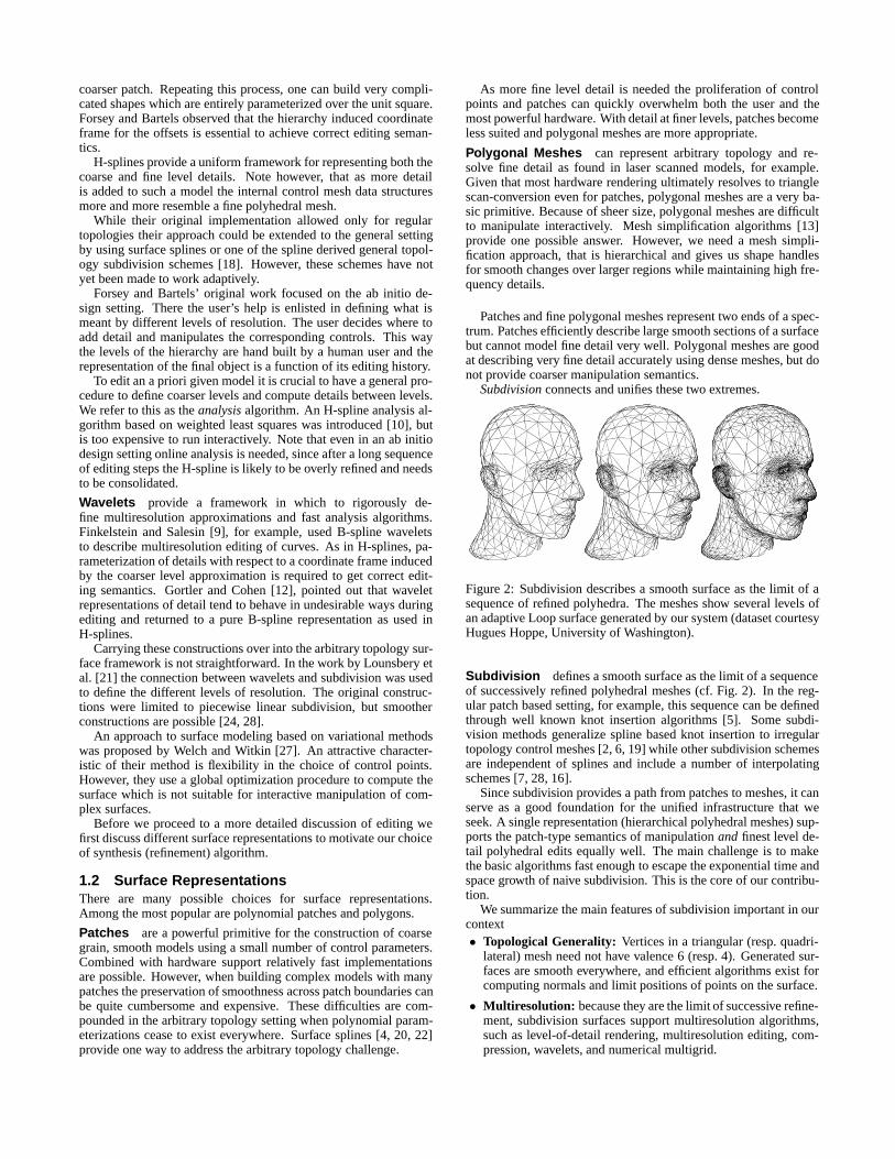
Subdivision connects and unifies these two extremes.

Figure 2: Subdivision describes a smooth surface as the limit of asequence of refined polyhedra. The meshes show several levels ofan adaptive Loop surface generated by our system (dataset courtesyHugues Hoppe, University of Washington).

Subdivision defines a smooth surface as the limit of a sequenceof successively refined polyhedral meshes (cf. Fig. 2). In the reg-ular patch based setting, for example, this sequence can be definedthrough well known knot insertion algorithms [5]. Some subdi-vision methods generalize spline based knot insertion to irregulartopology control meshes [2, 6, 19] while other subdivision schemesare independent of splines and include a number of interpolatingschemes [7, 28, 16].

Since subdivision provides a path from patches to meshes, it canserve as a good foundation for the unified infrastructure that weseek. A single representation (hierarchical polyhedral meshes) sup-ports the patch-type semantics of manipulation and finest level de-tail polyhedral edits equally well. The main challenge is to makethe basic algorithms fast enough to escape the exponential time andspace growth of naive subdivision. This is the core of our contribu-tion.

We summarize the main features of subdivision important in ourcontext• Topological Generality: Vertices in a triangular (resp. quadri-

lateral) mesh need not have valence 6 (resp. 4). Generated sur-faces are smooth everywhere, and efficient algorithms exist forcomputing normals and limit positions of points on the surface.

• Multiresolution: because they are the limit of successive refine-ment, subdivision surfaces support multiresolution algorithms,such as level-of-detail rendering, multiresolution editing, com-pression, wavelets, and numerical multigrid.

• Simplicity: subdivision algorithms are simple: the finer meshis built through insertion of new vertices followed by localsmoothing.

• Uniformity of Representation: subdivision provides a singlerepresentation of a surface at all resolution levels. Boundariesand features such as creases can be resolved through modifiedrules [14, 25], reducing the need for trim curves, for example.

1.3 Our ContributionAside from our perspective, which unifies the earlier approaches,our major contribution—and the main challenge in this program—is the design of highly adaptive and dynamic data structures andalgorithms, which allow the system to function across a range ofcomputational resources from PCs to workstations, delivering asmuch interactive fidelity as possible with a given polygon render-ing performance. Our algorithms work for the class of 1-ring sub-division schemes (definition see below) and we demonstrate theirperformance for the concrete case of Loop’s subdivision scheme.

The particulars of those algorithms will be given later, but Fig. 3already gives a preview of how the different algorithms make upthe editing system. In the next sections we first talk in more detailabout subdivision, smoothing, and multiresolution transforms.

Adaptive render

Initial mesh

Render

Select group of verticesat level i

Adaptive analysis

Begin dragging

Create dependentsubmesh

DragRelease selection

Local analysis Local synthesis

Render

Adaptive synthesis

Figure 3: The relationship between various procedures as the usermoves a set of vertices.

2 SubdivisionWe begin by defining subdivision and fixing our notation. There are2 points of view that we must distinguish. On the one hand we aredealing with an abstract graph and perform topological operationson it. On the other hand we have a mesh which is the geometricobject in 3-space. The mesh is the image of a map defined on thegraph: it associates a point in 3D with every vertex in the graph(cf. Fig. 4). A triangle denotes a face in the graph or the associatedpolygon in 3-space.

Initially we have a triangular graph T0 with vertices V 0. Byrecursively refining each triangle into 4 subtriangles we can builda sequence of finer triangulations Ti with vertices V i, i > 0(cf. Fig. 4). The superscript i indicates the level of triangles andvertices respectively. A triangle t ∈ Ti is a triple of indicest = {va, vb, vc} ⊂ V i.

The vertex sets are nested as V j ⊂ V i if j < i. We defineodd vertices on level i as Mi = V i+1 \ V i. V i+1 consists of twodisjoint sets: even vertices (V i) and odd vertices (Mi). We definethe level of a vertex v as the smallest i for which v ∈ V i. The levelof v is i+ 1 if and only if v ∈Mi.

T iVi

1 2

3

s (1)i

s (3)i

s (2)i

4

56

T i+1V i+1

1 2

3s (6)i+1 s (3)

i+1

s (5)i+1

s (1)i+1

s (4)i+1

s (2)i+1

refi

nem

ent subdivision

Mesh with pointsGraph with vertices

Maps to

Figure 4: Left: the abstract graph. Vertices and triangles are mem-bers of sets V i and T i respectively. Their index indicates the levelof refinement when they first appeared. Right: the mapping to themesh and its subdivision in 3-space.

With each set V i we associate a map, i.e., for each vertex v andeach level i we have a 3D point si(v) ∈ R3. The set si containsall points on level i, si = {si(v) | v ∈ V i}. Finally, a subdivisionscheme is a linear operator S which takes the points from level i topoints on the finer level i+ 1: si+1 = S si

Assuming that the subdivision converges, we can define a limitsurface σ as

σ = limk→∞

Sk s0.

σ(v) ∈ R3 denotes the point on the limit surface associated withvertex v.

In order to define our offsets with respect to a local frame we alsoneed tangent vectors and a normal. For the subdivision schemesthat we use, such vectors can be defined through the application oflinear operators Q and R acting on si so that qi(v) = (Qsi)(v)and ri(v) = (Rsi)(v) are linearly independent tangent vectors atσ(v). Together with an orientation they define a local orthonormalframe F i(v) = (ni(v), qi(v), ri(v)). It is important to note thatin general it is not necessary to use precise normals and tangentsduring editing; as long as the frame vectors are affinely related tothe positions of vertices of the mesh, we can expect intuitive editingbehavior.

1-ring at level i 1-ring at level i+1

Figure 5: An even vertex has a 1-ring of neighbors at each level ofrefinement (left/middle). Odd vertices—in the middle of edges—have 1-rings around each of the vertices at either end of their edge(right).

Next we discuss two common subdivision schemes, both ofwhich belong to the class of 1-ring schemes. In these schemespoints at level i+1 depend only on 1-ring neighborhoods of points

at level i. Let v ∈ V i (v even) then the point si+1(v) is a functionof only those si(vn), vn ∈ V i, which are immediate neighborsof v (cf. Fig. 5 left/middle). If m ∈ Mi (m odd), it is the vertexinserted when splitting an edge of the graph; we call such verticesmiddle vertices of edges. In this case the point si+1(m) is a func-tion of the 1-rings around the vertices at the ends of the edge (cf.Fig. 5 right).

a(k)

1

1

1

1

11

1

3 3

1

1

Figure 6: Stencils for Loop subdivision with unnormalized weightsfor even and odd vertices.

Loop is a non-interpolating subdivision scheme based on a gen-eralization of quartic triangular box splines [19]. For a given evenvertex v ∈ V i, let vk ∈ V i with 1 ≤ k ≤ K be its K 1-ring neighbors. The new point si+1(v) is defined as si+1(v) =(a(K)+K)−1(a(K) si(v) +

∑K

k=1si(vk)) (cf. Fig. 6), a(K) =

K(1−α(K))/α(K), and α(K) = 5/8−(3+2 cos(2π/K))2/64.For odd v the weights shown in Fig. 6 are used. Two inde-pendent tangent vectors t1(v) and t2(v) are given by tp(v) =∑K

k=1cos(2π(k + p)/K) si(vk).

Features such as boundaries and cusps can be accommodatedthrough simple modifications of the stencil weights [14, 25, 29].

Butterfly is an interpolating scheme, first proposed by Dyn etal. [7] in the topologically regular setting and recently general-ized to arbitrary topologies [28]. Since it is interpolating we havesi(v) = σ(v) for v ∈ V i even. The exact expressions for oddvertices depend on the valence K and the reader is referred to theoriginal paper for the exact values [28].

For our implementation we have chosen the Loop scheme, sincemore performance optimizations are possible in it. However, thealgorithms we discuss later work for any 1-ring scheme.

3 Multiresolution TransformsSo far we only discussed subdivision, i.e., how to go from coarse tofine meshes. In this section we describe analysis which goes fromfine to coarse.

We first need smoothing, i.e., a linear operation H to build asmooth coarse mesh at level i− 1 from a fine mesh at level i:

si−1 = H si.

Several options are available here:• Least squares: One could define analysis to be optimal in the

least squares sense,

minsi−1‖si − S si−1‖2.

The solution may have unwanted undulations and is too expen-sive to compute interactively [10].

• Fairing: A coarse surface could be obtained as the solution toa global variational problem. This is too expensive as well. Analternative is presented by Taubin [26], who uses a local non-shrinking smoothing approach.

Because of its computational simplicity we decided to use a versionof Taubin smoothing. As before let v ∈ V i have K neighborsvk ∈ V i. Use the average, si(v) = K−1

∑K

k=1si(vk), to define

the discrete Laplacian L(v) = si(v)− si(v). On this basis Taubingives a Gaussian-like smoother which does not exhibit shrinkage

H := (I + µL) (I + λL).

With subdivision and smoothing in place, we can describe thetransform needed to support multiresolution editing. Recall thatfor multiresolution editing we want the difference between succes-sive levels expressed with respect to a frame induced by the coarserlevel, i.e., the offsets are relative to the smoother level.

With each vertex v and each level i > 0 we associate a detailvector, di(v) ∈ R3. The set di contains all detail vectors on level i,di = {di(v) | v ∈ V i}. As indicated in Fig. 7 the detail vectorsare defined as

di = (F i)t (si − S si−1) = (F i)t (I − S H) si,

i.e., the detail vectors at level i record how much the points at leveli differ from the result of subdividing the points at level i− 1. Thisdifference is then represented with respect to the local frame Fi toobtain coordinate independence.

Since detail vectors are sampled on the fine level mesh V i, thistransformation yields an overrepresentation in the spirit of the Burt-Adelson Laplacian pyramid [1]. The only difference is that thesmoothing filters (Taubin) are not the dual of the subdivision filter(Loop). Theoretically it would be possible to subsample the detailvectors and only record a detail per odd vertex of Mi−1. This iswhat happens in the wavelet transform. However, subsampling thedetails severely restricts the family of smoothing operators that canbe used.

t(F )

id

SubdivisionSmoothing

s -Ssis

i-1s

i-1ii

Figure 7: Wiring diagram of the multiresolution transform.

4 Algorithms and ImplementationBefore we describe the algorithms in detail let us recall the overallstructure of the mesh editor (cf. Fig 3). The analysis stage buildsa succession of coarser approximations to the surface, each withfewer control parameters. Details or offsets between successivelevels are also computed. In general, the coarser approximationsare not visible; only their control points are rendered. These con-trol points give rise to a virtual surface with respect to which theremaining details are given. Figure 8 shows wireframe representa-tions of virtual surfaces corresponding to control points on levels 0,1, and 2.

When an edit level is selected, the surface is represented inter-nally as an approximation at this level, plus the set of all finer leveldetails. The user can freely manipulate degrees of freedom at theedit level, while the finer level details remain unchanged relativeto the coarser level. Meanwhile, the system will use the synthesisalgorithm to render the modified edit level with all the finer detailsadded in. In between edits, analysis enforces consistency on theinternal representation of coarser levels and details (cf. Fig. 9).

The basic algorithms Analysis and Synthesis are verysimple and we begin with their description.

Let i = 0 be the coarsest and i = n the finest level with Nvertices. For each vertex v and all levels i finer than the first level

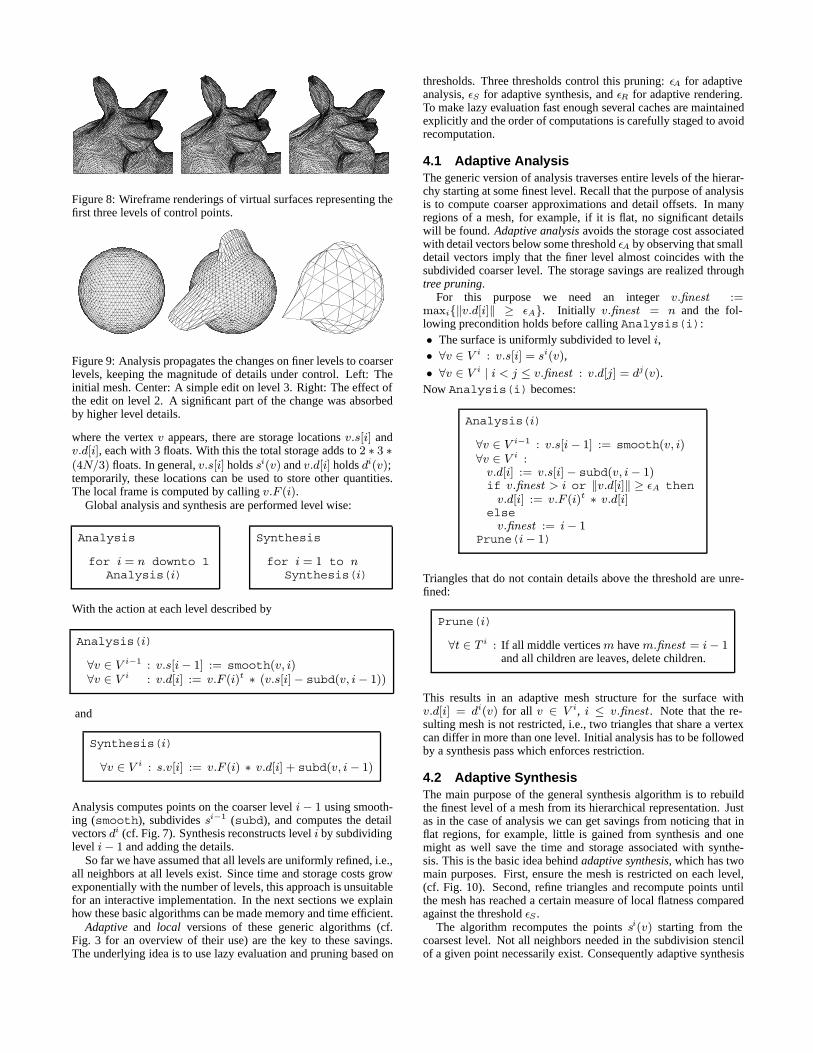
Figure 8: Wireframe renderings of virtual surfaces representing thefirst three levels of control points.

Figure 9: Analysis propagates the changes on finer levels to coarserlevels, keeping the magnitude of details under control. Left: Theinitial mesh. Center: A simple edit on level 3. Right: The effect ofthe edit on level 2. A significant part of the change was absorbedby higher level details.

where the vertex v appears, there are storage locations v.s[i] andv.d[i], each with 3 floats. With this the total storage adds to 2 ∗ 3 ∗(4N/3) floats. In general, v.s[i] holds si(v) and v.d[i] holds di(v);temporarily, these locations can be used to store other quantities.The local frame is computed by calling v.F (i).

Global analysis and synthesis are performed level wise:

Analysis

for i = n downto 1Analysis(i)

Synthesis

for i = 1 to nSynthesis(i)

With the action at each level described by

Analysis(i)

∀v ∈ V i−1 : v.s[i− 1] := smooth(v, i)∀v ∈ V i : v.d[i] := v.F (i)t ∗ (v.s[i]− subd(v, i− 1))

and

Synthesis(i)

∀v ∈ V i : s.v[i] := v.F (i) ∗ v.d[i] + subd(v, i− 1)

Analysis computes points on the coarser level i− 1 using smooth-ing (smooth), subdivides si−1 (subd), and computes the detailvectors di (cf. Fig. 7). Synthesis reconstructs level i by subdividinglevel i− 1 and adding the details.

So far we have assumed that all levels are uniformly refined, i.e.,all neighbors at all levels exist. Since time and storage costs growexponentially with the number of levels, this approach is unsuitablefor an interactive implementation. In the next sections we explainhow these basic algorithms can be made memory and time efficient.

Adaptive and local versions of these generic algorithms (cf.Fig. 3 for an overview of their use) are the key to these savings.The underlying idea is to use lazy evaluation and pruning based on

thresholds. Three thresholds control this pruning: εA for adaptiveanalysis, εS for adaptive synthesis, and εR for adaptive rendering.To make lazy evaluation fast enough several caches are maintainedexplicitly and the order of computations is carefully staged to avoidrecomputation.

4.1 Adaptive AnalysisThe generic version of analysis traverses entire levels of the hierar-chy starting at some finest level. Recall that the purpose of analysisis to compute coarser approximations and detail offsets. In manyregions of a mesh, for example, if it is flat, no significant detailswill be found. Adaptive analysis avoids the storage cost associatedwith detail vectors below some threshold εA by observing that smalldetail vectors imply that the finer level almost coincides with thesubdivided coarser level. The storage savings are realized throughtree pruning.

For this purpose we need an integer v.finest :=maxi{‖v.d[i]‖ ≥ εA}. Initially v.finest = n and the fol-lowing precondition holds before calling Analysis(i):• The surface is uniformly subdivided to level i,• ∀v ∈ V i : v.s[i] = si(v),

• ∀v ∈ V i | i < j ≤ v.finest : v.d[j] = dj(v).Now Analysis(i) becomes:

Analysis(i)

∀v ∈ V i−1 : v.s[i− 1] := smooth(v, i)∀v ∈ V i :v.d[i] := v.s[i]− subd(v, i− 1)if v.finest > i or ‖v.d[i]‖ ≥ εA thenv.d[i] := v.F (i)t ∗ v.d[i]

elsev.finest := i− 1

Prune(i− 1)

Triangles that do not contain details above the threshold are unre-fined:

Prune(i)

∀t ∈ T i : If all middle vertices m have m.finest = i− 1and all children are leaves, delete children.

This results in an adaptive mesh structure for the surface withv.d[i] = di(v) for all v ∈ V i, i ≤ v.finest . Note that the re-sulting mesh is not restricted, i.e., two triangles that share a vertexcan differ in more than one level. Initial analysis has to be followedby a synthesis pass which enforces restriction.

4.2 Adaptive SynthesisThe main purpose of the general synthesis algorithm is to rebuildthe finest level of a mesh from its hierarchical representation. Justas in the case of analysis we can get savings from noticing that inflat regions, for example, little is gained from synthesis and onemight as well save the time and storage associated with synthe-sis. This is the basic idea behind adaptive synthesis, which has twomain purposes. First, ensure the mesh is restricted on each level,(cf. Fig. 10). Second, refine triangles and recompute points untilthe mesh has reached a certain measure of local flatness comparedagainst the threshold εS .

The algorithm recomputes the points si(v) starting from thecoarsest level. Not all neighbors needed in the subdivision stencilof a given point necessarily exist. Consequently adaptive synthesis

i+1V

iV

V i V i

V

i

i+1

V i+1

T

Figure 10: A restricted mesh: the center triangle is in Ti and itsvertices in V i. To subdivide it we need the 1-rings indicated by thecircular arrows. If these are present the graph is restricted and wecan compute si+1 for all vertices and middle vertices of the centertriangle.

lazily creates all triangles needed for subdivision by temporarily re-fining their parents, then computes subdivision, and finally deletesthe newly created triangles unless they are needed to satisfy therestriction criterion. The following precondition holds before en-tering AdaptiveSynthesis:

• ∀t ∈ T j | 0 ≤ j ≤ i : t is restricted

• ∀v ∈ V j | 0 ≤ j ≤ v.depth : v.s[j] = sj(v)

where v.depth := maxi{si(v)has been recomputed}.

AdaptiveSynthesis

∀v ∈ V 0 : v.depth := 0for i = 0 to n− 1temptri := {}∀t ∈ T i :current := {}Refine(t, i,true)∀t ∈ temptri : if not t.restrict then

Delete children of t

The list temptri serves as a cache holding triangles from levelsj < i which are temporarily refined. A triangle is appended to thelist if it was refined to compute a value at a vertex. After processinglevel i these triangles are unrefined unless their t.restrict flag isset, indicating that a temporarily created triangle was later foundto be needed permanently to ensure restriction. Since triangles areappended to temptri , parents precede children. Deallocating thelist tail first guarantees that all unnecessary triangles are erased.

The function Refine(t, i, dir) (see below) creates children oft ∈ T i and computes the values Ssi(v) for the vertices and mid-dle vertices of t. The results are stored in v.s[i + 1]. The booleanargument dir indicates whether the call was made directly or recur-sively.

Refine(t, i, dir)

if t.leaf then Create children for t∀v ∈ t : if v.depth < i+ 1 thenGetRing(v, i)Update(v, i)∀m ∈ N(v, i+ 1, 1) :Update(m, i)if m.finest ≥ i+ 1 thenforced := true

if dir and Flat(t) < εS and not forced thenDelete children of t

else∀t ∈ current : t.restrict := true

Update(v, i)v.s[i+ 1] := subd(v, i)v.depth := i+ 1if v.finest ≥ i+ 1 thenv.s[i+ 1] += v.F (i+ 1) ∗ v.d[i+ 1]

The condition v.depth = i+ 1 indicates whether an earlier call toRefine already recomputed si+1(v). If not, call GetRing(v, i)and Update(v, i) to do so. In case a detail vector lives at v at leveli (v.finest ≥ i + 1) add it in. Next compute si+1(m) for mid-dle vertices on level i + 1 around v (m ∈ N(v, i + 1, 1), whereN(v, i, l) is the l-ring neighborhood of vertex v at level i). If mhas to be calculated, compute subd(m, i) and add in the detail if itexists and record this fact in the flag forced which will prevent unre-finement later. At this point, all si+1 have been recomputed for thevertices and middle vertices of t. Unrefine t and delete its childrenif Refine was called directly, the triangle is sufficiently flat, andnone of the middle vertices contain details (i.e., forced = false).The list current functions as a cache holding triangles from leveli − 1 which are temporarily refined to build a 1-ring around thevertices of t. If after processing all vertices and middle vertices oft it is decided that t will remain refined, none of the coarser-leveltriangles from current can be unrefined without violating restric-tion. Thus t.restrict is set for all of them. The function Flat(t)measures how close to planar the corners and edge middle verticesof t are.

Finally, GetRing(v, i) ensures that a complete ring of triangleson level i adjacent to the vertex v exists. Because triangles on leveli are restricted triangles all triangles on level i − 1 that contain vexist (precondition). At least one of them is refined, since other-wise there would be no reason to call GetRing(v, i). All othertriangles could be leaves or temporarily refined. Any triangle thatwas already temporarily refined may become permanently refinedto enforce restriction. Record such candidates in the current cachefor fast access later.

GetRing(v, i)

∀t ∈ T i−1 with v ∈ t :if t.leaf thenRefine(t, i− 1, false); temptri .append(t)t.restrict := false; t.temp := true

if t.temp thencurrent .append (t)

4.3 Local SynthesisEven though the above algorithms are adaptive, they are still run ev-erywhere. During an edit, however, not all of the surface changes.The most significant economy can be gained from performing anal-ysis and synthesis only over submeshes which require it.

Assume the user edits level l and modifies the points sl(v) forv ∈ V ∗l ⊂ V l. This invalidates coarser level values si and di forcertain subsets V ∗i ⊂ V i, i ≤ l, and finer level points si for subsetsV ∗i ⊂ V i for i > l. Finer level detail vectors di for i > l remaincorrect by definition. Recomputing the coarser levels is done bylocal incremental analysis described in Section 4.4, recomputingthe finer level is done by local synthesis described in this section.

The set of vertices V ∗i which are affected depends on the supportof the subdivision scheme. If the support fits into an m-ring aroundthe computed vertex, then all modified vertices on level i + 1 canbe found recursively as

V ∗i+1 =⋃

v∈V ∗iN(v, i+ 1,m).

We assume that m = 2 (Loop-like schemes) or m = 3 (Butterflytype schemes). We define the subtriangulation T∗i to be the subsetof triangles of T i with vertices in V ∗i.LocalSynthesis is only slightly modified from

AdaptiveSynthesis: iteration starts at level l and iter-ates only over the submesh T∗i.

4.4 Local Incremental AnalysisAfter an edit on level l local incremental analysis will recomputesi(v) and di(v) locally for coarser level vertices (i ≤ l) which areaffected by the edit. As in the previous section, we assume thatthe user edited a set of vertices v on level l and call V∗i the set ofvertices affected on level i. For a given vertex v ∈ V∗i we define

vf1

v7

v

v

1vv ve

f 2

e 2

6

v1

4

v5

v

v

v2

v3

Figure 11: Sets of even vertices affected through smoothing by ei-ther an even v or odd m vertex.

Ri−1(v) ⊂ V i−1 to be the set of vertices on level i − 1 affectedby v through the smoothing operator H . The sets V∗i can now bedefined recursively starting from level i = l to i = 0:

V ∗i−1 =⋃

v∈V ∗iRi−1(v).

The set Ri−1(v) depends on the size of the smoothing stencil andwhether v is even or odd (cf. Fig. 11). If the smoothing filteris 1-ring, e.g., Gaussian, then Ri−1(v) = {v} if v is even andRi−1(m) = {ve1, ve2} if m is odd. If the smoothing filter is 2-ring, e.g., Taubin, then Ri−1(v) = {v} ∪ {vk | 1 ≤ k ≤ K}if v is even and Ri−1(m) = {ve1, ve2, vf1, vf2} if v is odd. Be-cause of restriction, these vertices always exist. For v ∈ V i andv′ ∈ Ri−1(v) we let c(v, v′) be the coefficient in the analysis sten-cil. Thus

(H si)(v′) =∑

v|v′∈Ri−1(v)

c(v, v′)si(v).

This could be implemented by running over the v′ and each timecomputing the above sum. Instead we use the dual implementation,iterate over all v, accumulating (+=) the right amount to si(v′) forv′ ∈ Ri−1(v). In case of a 2-ring Taubin smoother the coefficientsare given by

c(v, v) = (1− µ) (1− λ) + µλ/6

c(v, vk) = µλ/6K

c(m, ve1) = ((1− µ)λ+ (1− λ)µ+ µλ/3)/K

c(m, vf1) = µλ/3K,

where for each c(v, v′), K is the outdegree of v′.The algorithm first copies the old points si(v) for v ∈ V ∗i and

i ≤ l into the storage location for the detail. If then propagatesthe incremental changes of the modified points from level l to thecoarser levels and adds them to the old points (saved in the detaillocations) to find the new points. Then it recomputes the detailvectors that depend on the modified points.

We assume that before the edit, the old points sl(v) for v ∈V ∗l were saved in the detail locations. The algorithm starts out bybuilding V ∗i−1 and saving the points si−1(v) for v ∈ V ∗i−1 inthe detail locations. Then the changes resulting from the edit arepropagated to level i − 1. Finally S si−1 is computed and used toupdate the detail vectors on level i.

LocalAnalysis(i)

∀v ∈ V ∗i : ∀v′ ∈ Ri−1(v) :V ∗i−1 ∪= {v′}v′.d[i− 1] := v′.s[i− 1]∀v ∈ V ∗i : ∀v′ ∈ Ri−1(v) :v′.s[i− 1] += c(v, v′) ∗ (v.s[i]− v.d[i])∀v ∈ V ∗i−1 :v.d[i] = v.F (i)t ∗ (v.s[i]− subd(v, i− 1))∀m ∈ N(v, i, 1) :m.d[i] = m.F (i)t ∗ (m.s[i]− subd(m, i− 1))

Note that the odd points are actually computed twice. For the Loopscheme this is less expensive than trying to compute a predicate toavoid this. For Butterfly type schemes this is not true and one canavoid double computation by imposing an ordering on the triangles.The top level code is straightforward:

LocalAnalysis

∀v ∈ V ∗l : v.d[l] := v.s[l]for i := l downto 0LocalAnalysis(i)

It is difficult to make incremental local analysis adaptive, as it isformulated purely in terms of vertices. It is, however, possible toadaptively clean up the triangles affected by the edit and (un)refinethem if needed.

4.5 Adaptive RenderingThe adaptive rendering algorithm decides which triangles will bedrawn depending on the rendering performance available and levelof detail needed.

The algorithm uses a flag t.draw which is initialized to false,but set to true as soon as the area corresponding to t is drawn.This can happen either when t itself gets drawn, or when a set ofits descendents, which cover t, is drawn. The top level algorithmloops through the triangles starting from the level n− 1. A triangle

is always responsible for drawing its children, never itself, unless itis a coarsest-level triangle.

AdaptiveRender

for i = n− 1 downto 0∀t ∈ T i : if not t.leaf thenRender(t)

∀t ∈ T 0 : if not t.draw thendisplaylist.append(t)

T-vertex

Figure 12: Adaptive rendering: On the left 6 triangles from level i,one has a covered child from level i + 1, and one has a T-vertex.On the right the result from applying Render to all six.

The Render(t) routine decides whether the children of t have to bedrawn or not (cf. Fig.12). It uses a function edist(m)which mea-sures the distance between the point corresponding to the edge’smiddle vertex m, and the edge itself. In the when case any of thechildren of t are already drawn or any of its middle vertices are farenough from the plane of the triangle, the routine will draw the restof the children and set the draw flag for all their vertices and t. Italso might be necessary to draw a triangle if some of its middlevertices are drawn because the triangle on the other side decidedto draw its children. To avoid cracks, the routine cut(t) will cutt into 2, 3, or 4, triangles depending on how many middle verticesare drawn.

Render(t)

if (∃ c ∈ t.child | c.draw = trueor ∃m ∈ t.mid vertex | edist(m) > εD) then∀c ∈ t.child :if not c.draw then

displaylist.append (c)∀v ∈ c : v.draw := true

t.draw := trueelse if ∃m ∈ t.mid vertex | m.draw = true∀t′ ∈ cut(t) : displaylist.append(t′)t.draw := true

4.6 Data Structures and CodeThe main data structure in our implementation is a forest of trian-gular quadtrees. Neighborhood relations within a single quadtreecan be resolved in the standard way by ascending the tree to theleast common parent when attempting to find the neighbor across agiven edge. Neighbor relations between adjacent trees are resolvedexplicitly at the level of a collection of roots, i.e., triangles of acoarsest level graph. This structure also maintains an explicit rep-resentation of the boundary (if any). Submeshes rooted at any levelcan be created on the fly by assembling a new graph with some setof triangles as roots of their child quadtrees. It is here that the ex-plicit representation of the boundary comes in, since the actual trees

are never copied, and a boundary is needed to delineate the actualsubmesh.

The algorithms we have described above make heavy use ofcontainer classes. Efficient support for sets is essential for a fastimplementation and we have used the C++ Standard Template Li-brary. The mesh editor was implemented using OpenInventor andOpenGL and currently runs on both SGI and Intel PentiumProworkstations.

Figure 13: On the left are two meshes which are uniformly sub-divided and consist of 11k (upper) and 9k (lower) triangles. Onthe right another pair of meshes mesh with approximately the samenumbers of triangles. Upper and lower pairs of meshes are gen-erated from the same original data but the right meshes were op-timized through suitable choice of εS . See the color plates for acomparison between the two under shading.

5 ResultsIn this section we show some example images to demonstrate vari-ous features of our system and give performance measures.

Figure 13 shows two triangle mesh approximations of the Ar-madillo head and leg. Approximately the same number of trianglesare used for both adaptive and uniform meshes. The meshes on theleft were rendered uniformly, the meshes on the right were renderedadaptively. (See also color plate 15.)

Locally changing threshold parameters can be used to resolve anarea of interest particularly well, while leaving the rest of the meshat a coarse level. An example of this “lens” effect is demonstratedin Figure 14 around the right eye of the Mannequin head. (See alsocolor plate 16.)

We have measured the performance of our code on two plat-forms: an Indigo R10000@175MHz with Solid Impact graphics,and a PentiumPro@200MHz with an Intergraph Intense 3D board.

We used the Armadillo head as a test case. It has approximately172000 triangles on 6 levels of subdivision. Display list creationtook 2 seconds on the SGI and 3 seconds on the PC for the fullmodel. We adjusted εR so that both machines rendered models at5 frames per second. In the case of the SGI approximately 113,000triangles were rendered at that rate. On the PC we achieved 5frames per second when the rendering threshold had been raisedenough so that an approximation consisting of 35000 polygons wasused.

The other important performance number is the time it takes torecompute and re-render the region of the mesh which is changingas the user moves a set of control points. This submesh is renderedin immediate mode, while the rest of the surface continues to berendered as a display list. Grabbing a submesh of 20-30 faces (atypical case) at level 0 added 250 mS of time per redraw, at level 1it added 110 mS and at level 2 it added 30 mS in case of the SGI.The corresponding timings for the PC were 500 mS, 200 mS and60 mS respectively.

Figure 14: It is easy to change εS locally. Here a “lens” was appliedto the right eye of the Mannequin head with decreasing εS to forcevery fine resolution of the mesh around the eye.

6 Conclusion and Future ResearchWe have built a scalable system for interactive multiresolution edit-ing of arbitrary topology meshes. The user can either start fromscratch or from a given fine detail mesh with subdivision connec-tivity. We use smooth subdivision combined with details at eachlevel as a uniform surface representation across scales and arguethat this forms a natural connection between fine polygonal meshesand patches. Interactivity is obtained by building both local andadaptive variants of the basic analysis, synthesis, and rendering al-gorithms, which rely on fast lazy evaluation and tree pruning. Thesystem allows interactive manipulation of meshes according to thepolygon performance of the workstation or PC used.

There are several avenues for future research:• Multiresolution transforms readily connect with compression.

We want to be able to store the models in a compressed formatand use progressive transmission.

• Features such as creases, corners, and tension controls can easilybe added into our system and expand the users’ editing toolbox.

• Presently no real time fairing techniques, which lead to moreintuitive coarse levels, exist.

• In our system coarse level edits can only be made by draggingcoarse level vertices. Which vertices live on coarse levels iscurrently fixed because of subdivision connectivity. Ideally theuser should be able to dynamically adjust this to make coarselevel edits centered at arbitrary locations.

• The system allows topological edits on the coarsest level. Algo-rithms that allow topological edits on all levels are needed.

• An important area of research relevant for this work is genera-tion of meshes with subdivision connectivity from scanned dataor from existing models in other representations.

AcknowledgmentsWe would like to thank Venkat Krishnamurthy for providing theArmadillo dataset. Andrei Khodakovsky and Gary Wu helped be-yond the call of duty to bring the system up. The research wassupported in part through grants from the Intel Corporation, Mi-crosoft, the Charles Lee Powell Foundation, the Sloan Founda-tion, an NSF CAREER award (ASC-9624957), and under a MURI(AFOSR F49620-96-1-0471). Other support was provided by theNSF STC for Computer Graphics and Scientific Visualization.

References[1] BURT, P. J., AND ADELSON, E. H. Laplacian Pyramid as a

Compact Image Code. IEEE Trans. Commun. 31, 4 (1983),532–540.

[2] CATMULL, E., AND CLARK, J. Recursively Generated B-Spline Surfaces on Arbitrary Topological Meshes. ComputerAided Design 10, 6 (1978), 350–355.

[3] CERTAIN, A., POPOVIC, J., DEROSE, T., DUCHAMP, T.,SALESIN, D., AND STUETZLE, W. Interactive Multiresolu-tion Surface Viewing. In SIGGRAPH 96 Conference Proceed-ings, H. Rushmeier, Ed., Annual Conference Series, 91–98,Aug. 1996.

[4] DAHMEN, W., MICCHELLI, C. A., AND SEIDEL, H.-P. Blossoming Begets B-Splines Bases Built Better by B-Patches. Mathematics of Computation 59, 199 (July 1992),97–115.

[5] DE BOOR, C. A Practical Guide to Splines. Springer, 1978.[6] DOO, D., AND SABIN, M. Analysis of the Behaviour of

Recursive Division Surfaces near Extraordinary Points. Com-puter Aided Design 10, 6 (1978), 356–360.

[7] DYN, N., LEVIN, D., AND GREGORY, J. A. A ButterflySubdivision Scheme for Surface Interpolation with TensionControl. ACM Trans. Gr. 9, 2 (April 1990), 160–169.

[8] ECK, M., DEROSE, T., DUCHAMP, T., HOPPE, H., LOUNS-BERY, M., AND STUETZLE, W. Multiresolution Analysis ofArbitrary Meshes. In Computer Graphics Proceedings, An-nual Conference Series, 173–182, 1995.

[9] FINKELSTEIN, A., AND SALESIN, D. H. MultiresolutionCurves. Computer Graphics Proceedings, Annual ConferenceSeries, 261–268, July 1994.

[10] FORSEY, D., AND WONG, D. Multiresolution Surface Re-construction for Hierarchical B-splines. Tech. rep., Universityof British Columbia, 1995.

[11] FORSEY, D. R., AND BARTELS, R. H. Hierarchical B-SplineRefinement. Computer Graphics (SIGGRAPH ’88 Proceed-ings), Vol. 22, No. 4, pp. 205–212, August 1988.

[12] GORTLER, S. J., AND COHEN, M. F. Hierarchical and Vari-ational Geometric Modeling with Wavelets. In ProceedingsSymposium on Interactive 3D Graphics, May 1995.

[13] HOPPE, H. Progressive Meshes. In SIGGRAPH 96 Con-ference Proceedings, H. Rushmeier, Ed., Annual ConferenceSeries, 99–108, August 1996.

[14] HOPPE, H., DEROSE, T., DUCHAMP, T., HALSTEAD, M.,JIN, H., MCDONALD, J., SCHWEITZER, J., AND STUET-ZLE, W. Piecewise Smooth Surface Reconstruction. In Com-puter Graphics Proceedings, Annual Conference Series, 295–302, 1994.

[15] HOPPE, H., DEROSE, T., DUCHAMP, T., MCDONALD, J.,AND STUETZLE, W. Mesh Optimization. In ComputerGraphics (SIGGRAPH ’93 Proceedings), J. T. Kajiya, Ed.,vol. 27, 19–26, August 1993.

[16] KOBBELT, L. Interpolatory Subdivision on Open Quadrilat-eral Nets with Arbitrary Topology. In Proceedings of Euro-graphics 96, Computer Graphics Forum, 409–420, 1996.

Figure 15: Shaded rendering (OpenGL) of the meshes in Figure 13.

Figure 16: Shaded rendering (OpenGL) of the meshes in Figure 14.

[17] KRISHNAMURTHY, V., AND LEVOY, M. Fitting Smooth Sur-faces to Dense Polygon Meshes. In SIGGRAPH 96 Confer-ence Proceedings, H. Rushmeier, Ed., Annual Conference Se-ries, 313–324, August 1996.

[18] KURIHARA, T. Interactive Surface Design Using RecursiveSubdivision. In Proceedings of Communicating with VirtualWorlds. Springer Verlag, June 1993.

[19] LOOP, C. Smooth Subdivision Surfaces Based on Triangles.Master’s thesis, University of Utah, Department of Mathemat-ics, 1987.

[20] LOOP, C. Smooth Spline Surfaces over Irregular Meshes. InComputer Graphics Proceedings, Annual Conference Series,303–310, 1994.

[21] LOUNSBERY, M., DEROSE, T., AND WARREN, J. Multires-olution Analysis for Surfaces of Arbitrary Topological Type.Transactions on Graphics 16, 1 (January 1997), 34–73.

[22] PETERS, J. C1 Surface Splines. SIAM J. Numer. Anal. 32, 2(1995), 645–666.

[23] PULLI, K., AND LOUNSBERY, M. Hierarchical Editing andRendering of Subdivision Surfaces. Tech. Rep. UW-CSE-97-04-07, Dept. of CS&E, University of Washington, Seattle,WA, 1997.

[24] SCHRODER, P., AND SWELDENS, W. Spherical wavelets:Efficiently representing functions on the sphere. ComputerGraphics Proceedings, (SIGGRAPH 95) (1995), 161–172.

[25] SCHWEITZER, J. E. Analysis and Application of SubdivisionSurfaces. PhD thesis, University of Washington, 1996.

[26] TAUBIN, G. A Signal Processing Approach to Fair SurfaceDesign. In SIGGRAPH 95 Conference Proceedings, R. Cook,Ed., Annual Conference Series, 351–358, August 1995.

[27] WELCH, W., AND WITKIN, A. Variational surface modeling.In Computer Graphics (SIGGRAPH ’92 Proceedings), E. E.Catmull, Ed., vol. 26, 157–166, July 1992.

[28] ZORIN, D., SCHRODER, P., AND SWELDENS, W. Interpo-lating Subdivision for Meshes with Arbitrary Topology. Com-puter Graphics Proceedings (SIGGRAPH 96) (1996), 189–192.

[29] ZORIN, D. N. Subdivision and Multiresolution Surface Rep-resentations. PhD thesis, Caltech, Pasadena, California, 1997.