Interaction of Fluids with Deformable Solids

Matthias Muller Simon Schirm Matthias Teschner Bruno Heidelberger Markus GrossETH Zurich, Switzerland

AbstractIn this paper, we present a method for simulat-ing the interaction of fluids with deformable solids.The method is designed for the use in interactivesystems such as virtual surgery simulators wherethe real-time interplay of liquids and surroundingtissue is important.In computer graphics, a variety of techniques havebeen proposed to model liquids and deformable ob-jects at interactive rates. As important as the plau-sible animation of these substances is the fast andstable modeling of their interaction. The methodwe describe in this paper models the exchangeof momentum between Lagrangian particle-basedfluid models and solids represented by polygonalmeshes. To model the solid-fluid interaction weuse virtual boundary particles. They are placed onthe surface of the solid objects according to Gaus-sian quadrature rules allowing the computation ofsmooth interaction potentials that yield stable sim-ulations. We demonstrate our approach in an in-teractive simulation environment for fluids and de-formable solids.

Keywords: smoothed particle hydrodynamics (SPH), finiteelement method (FEM), fluid-solid interaction

1 IntroductionInteractive physically based simulation is a rapidly growingresearch area with an increasing number of applications, e. g.in games and computational surgery. In these simulation en-vironments, deformable objects play an important role. Forthe simulation of deformable solids, a variety of models havebeen proposed ranging from efficient mass-spring approachesto methods based on the physically more accurate Finite Ele-ment Method (FEM). Some of these methods allow the simu-lation of elastically and plastically deformable solids at inter-active speed.

More recently, there has been an increased interest in ef-ficient methods for the realistic simulation of fluids. Theseapproaches can be employed to represent blood or other liq-uids. Besides deformable models, they play an essential rolein applications such as surgery simulation. So far, only a fewinteractive methods for the simulation of fluids with free sur-faces have been proposed.

With the ability to simulate both, deformable solids andfluids, a new problem has been introduced, namely the mod-

eling of the interaction of these structures. An interactionmodel suitable for the use in interactive environments needsto be computationally efficient and the generated interactionforces must not induce any instabilities to the dynamic simu-lation.

In this paper, we present a new technique to model in-teractions between particle based fluids and mesh baseddeformable solids which meets these constraints. Wepresent our interaction model with fluids represented by aSmoothed Particle Hydrodynamics approach (SPH) and withdeformable solids represented by a Finite Element approach.However, the general interaction model we propose workswith any type of deformation technique as long as the ob-ject surface is represented by a polygonal mesh and the fluidby Lagrangian particles.

2 Related WorkThe majority of publications in the area of physically basedanimation focuses on physical systems of one single type.Deformable objects are interesting to study in their own right.In fluid simulation, on the other hand, boundary conditionsare often considered a necessary but not a central issue. Theyare typically derived from simple geometric primitives. Ourmethod connects these two areas of research.

In the field of computer graphics, a large number of meshbased methods for the physically based simulation of de-formable objects have been proposed since the pioneering pa-per of Terzopoulos [1]. Early techniques were mostly basedon mass-spring systems, which are still popular for clothsimulation [2, 3]. More recent methods discretize continu-ous elasticity equations via the Boundary Element Method(BEM) [4] or the Finite Element Method (FEM) [5, 6, 7].

Since T. Reeves [8] introduced particle systems as a tech-nique for modeling fuzzy objects twenty years ago, a varietyof special purpose, partice based fluid simulation techniqueshave been developed in the field of computer graphics. Des-brun and Cani [9] where among the first to use Smoothed Par-ticle Hydrodynamics (SPH) [10] to derive interaction forcesfor particle systems. They added space-adaptivity in [11].Later, Stora et al. [12] used a similar particle based model toanimate lava flows. In [13], Muller et al. derived inter parti-cle forces from SPH and the Navier Stokes equation to sim-ulate water with free surfaces at interactive rates. Recently,Premoze et al. [14] introduced the Moving-Particle Semi-Implicit (MPS) method to computer graphics for the simula-tion of fluids. As a mesh-free method, it is closely related toSPH but in contrast to standard SPH, it allows the simulation

1

Figure 1: A box falls into a pool and generates a shock wave that causes the pool to fracture.

of incompressible fluids. In all these papers, boundary con-ditions are not treated explicitly. The fluids typically interactwith solid walls or the ground.

Genevaux et al. [15] address the interaction problem ex-plicitly. They propose a method to simulate the interactionbetween solids represented by mass-spring networks and anEulerian fluid grid by applying spring forces to the mass-lessmarker particles in the fluid and the nodes of the mass-springnetwork. However, solids are typically represented by coarsemeshes, especially in interactive simulations. Thus, the nodesof a mass-spring network are not very well suited for the ap-plication of interaction forces. Therefore, Monaghan, one ofthe founders of the SPH formalism, uses special boundaryor ghost particles on fixed borders to model interactions [16].The idea of ghost particles was picked up in several followingprojects including our own. The key contribution of our pa-per is to place these ghost particles onto boundary triangles ofdeformable objects and to derive their locations and weightsaccording to Gauss integration [17], which allows to modelfluid-solid interactions stably at interactive rates.

3 Physical Problem DescriptionIn physically based animation, we are interested in the sim-ulation of macroscopic effects at interactive speed. There-fore, we consider macroscopic models for both, solids andfluids. Materials, which are homogeneous at the macroscopiclevel, can mathematically be described as a continuum [18].Thereby, quantities such as the density ρ, viscosity µ, defor-mation u or velocity v are all mathematically expressed bycontinuous functions over space and time. A physical modelrelates these quantities to each other via partial differentialequations (PDEs). The mechanical behavior of an elasticsolid can be described by the following equation

ρ∂2

∂t2u = ∇ · σs(u) + f , (1)

which expresses Newton’s equation of motion, namely thatthe change of momentum on the left hand side is equal to theinternal elastic forces due to the stresses σs plus the externallyapplied body forces f . The stresses σs are functions of thedisplacements u. The equation is in Lagrangian form sincethe displacement vectors u follow the material points.

Similarly, mechanical properties of incompressible Newto-nian fluids can be described by the following two equationsin Eulerian form where fluid quantities are observed in a fixedcoordinate frame

ρ

(∂v∂t

+ v · ∇v)

= ∇ · σf (v) + f (2)

∇ · v = 0. (3)

Equation (2) again states that the change of momentum equalsthe internal forces derived from the stresses σf plus the ex-ternally applied body forces f . The stress tensor σf =2µε(v)− pI is composed of the viscosity stress and the pres-sure stress. The viscosity stress is dependent on the viscosityµ and the strain rate tensor ε while the pressure stress only de-pends on the scalar pressure p. For an incompressible fluid,the velocity field is divergence free (Eq. (3)).

Comparison of the right hand side of the two equationsof motion (1) and (2) reveals, that the Eulerian descriptionmakes the additional convection term v · ∇v necessary. InSec. 4, we discuss numerical methods to solve both equationsof motion. For fluids we focus on particle based methods suchas SPH for which this term can be omitted.

3.1 Boundary Conditions

Materials such as fluids or solids are bounded by spatial lim-its. The behavior of materials at these limits is defined byboundary conditions. The boundary conditions relate thequantities of the two adjacent materials to each other at the in-terface. In the case of fluid-solid interaction, the geometricaldomain of the interface Γ is defined as a surface between thevolumetric solid continuum and the volumetric fluid contin-uum (see Fig. 2(a)). We focus on three main types of bound-ary conditions.

3.2 No-Penetration Condition

If the solid is considered to be impermeable, no fluid elementis allowed to cross the boundary, which is described in thefollowing equation:

(∂

∂tu − v) · n = 0 at the boundary Γ, (4)

where n is the normal on Γ (see Fig. 2(b)). The equationstates that the components of the velocities of the fluid andthe deformable object perpendicular to Γ are equal.

3.3 No-Slip Condition

The no-slip condition models friction between the fluid andthe solid (see Fig. 2(c)). It holds for most fluids-solid surfacesand it states that the velocity components tangential to thefluid surface have to be equal, thus

(∂

∂tu − v) × n = 0 at the boundary Γ. (5)

If both independent boundary conditions (4) and (5) hold,we simply have ∂

∂tu = v at the boundary, i.e. both materialshave the same velocity at the boundary.

2

3.4 Actio = ReactioNewton’s Third Law demands the continuity of stresses σs

and σf throughout the boundary (see Fig. 2(d)). In otherwords, the traction forces of the solid gf must be oppositeto the traction forces of the fluid gs on the boundary Γ

gs = σsn = σf (−n) = −gf , (6)

where n is the outward normal on the solid and −n the out-ward normal on the fluid.

(a) (b) (c)

u v

Γsolid fluid

n

v

u.

n

vu.

(d)

n

σsσf

-n

gs

gf

Figure 2: Boundary conditions: (a) A solid object is deformedby a displacement field u and interacts with a fluid whosevelocity field is v. The no-penetration condition is shownin image (b) where u is the time derivative of u. Image (c)illustrates the no-slip condition and image (d) Newton’s ThirdLaw.

4 Computational ModelThe continuous equations and boundary conditions describedin the previous section need to be discretized in space andtime via a numerical method before they can be used in acomputer simulation. We do not go into the details of howequation (1) for elastic objects can be solved numerically. Forpossible solutions using the Finite Element Method (FEM)we refer the reader to [19], [6] or [7]. All we require for ourinteraction method to work is

• that the solid object is represented by a mesh and

• that the displacements, velocities and forces are carriedby the nodes of the mesh.

Most of the methods used in computer graphics to simulatedeformable objects meet these constraints including mass-spring systems, the Finite Volume Method (FVM) and theBoundary Element Method (BEM).

For the simulation of fluids, two main numerical methodshave been used in the field of physically based animation sofar, namely Eulerian grid-based approaches [20, 21, 22] andLagrangian methods based on particles (see Sec. 2). In thispaper we concentrate on Lagrangian methods because theyallow fluids with free surfaces to move freely in space whilein the Eulerian case fluid computations are restricted to aspatially fixed and bounded grid. From the fluid simulationmethod we require

• that the fluid is represented by a set of particles and

• that positions, velocities and internal forces are carriedby the particles.

Interaction modeling, thus, reduces to the problem of simu-lating the interaction between particles and triangulated sur-faces.

(a) (b)

(c) (d)

Figure 3: (a) Iso surfaces of the Euclidean distance field of apiecewise linear curve (blue) with discontinuous first deriva-tives near concavities. (b) Weighted sums yield smooth isosurfaces with bulges. (c) Normalization does not remove theartifact. (d) Convolution yields bulge-free smooth iso sur-faces.

4.1 Interaction of Particles with TrianglesIn physics, interaction potentials of two objects always de-pend on the distance between them. While the Euclidean dis-tance between two points is uniquely defined, the distancebetween a point and a triangle or a point and a triangulatedsurface needs to be defined. Let us define the distance of apoint p from a triangle t as

d(p, t) = minx∈t

|p − x|, (7)

and the distance of a point p from a triangulated surface T as

d(p, T ) = mint∈T

d(p, t). (8)

Figure 3(a) shows several isosurfaces of the resulting distancefield which is C0 continuous everywhere. Unfortunately,concavities as well as close disconnected meshes generatediscontinuous first derivatives of the distance field. Those dis-continuities lead to discontinuous derivatives in forces sincethe forces depend on the distance field. A force field withdiscontinuous first derivatives, in turn, yields artifacts suchas the so called cooking of particles in concave regions andreduced stability of the simulation.

The source of the discontinuity in the first derivatives is theminimum operator in Eqn. (8). One way to remove the prob-lem is to replace the minimum by a weighted sum. Let thekernel W (d, h) ∈ C1 be a positive smooth monotonously de-creasing function which is zero for d ≥ h and has a vanishingderivative at d = h. We can then define the potential Φ of apoint p with respect to a triangulated surface T which is nota Eucledian distance anymore

Φ(p, T ) =∑t∈T

d(p, t)W (d(p, t), h), (9)

but which is C0 and C1 continuous everywhere. However, asFig. 3(b) shows, the resulting field is distorted near triangleboundaries. This effect can be removed by normalization

Φ(p, T ) ={

1wΦ(p, T ) if w > 00 otherwise,

(10)

3

where w =∑

t∈T W (d(p, t), h). Unfortunately, normaliza-tion just distributes the distortions to adjacent regions of tri-angle interfaces as Fig. 3(c) shows. Another difficulty intro-duced by the weighted field method is the choice of the sup-port radius h with respect to the size of the features of theboundary T . For large supports, small features are smoothedout while small supports reduce the interaction range of T .

4.2 Convolution SurfacesThe problems mentioned in the previous section are wellknown in the field of implicit surface modeling introducedby Blinn [23]. An elegant way to generate a bulge-free sur-face around a skeleton S, is to define a scalar function FS asthe convolution

FS(p) =∫x∈S

W (p − x)dx. (11)

The implicit surface is defined by selecting an iso-surface ofFS . By replacing the skeleton S with the triangulated surfaceT we get a smooth potential field around T (see Fig. 3(d)).The problem with the weighted sum approach arises whenwhen multiple triangles meet. In this case, all triangles con-tribute as a whole to the sum and generate bulges. In contrast,the convolution integral sums up infinitesimal parts of theskeleton each properly weighted (see Fig. 4). When the con-volution integral is used, the interaction of p with the surfaceT is modeled as the interaction of p with all the infinitesimalpoints in T . For skeletal elements other than points, the inte-gral in Eqn. (11) yields complex computations. Approachesto approximate this integral were proposed by Bloomenthal[24] and Sherstyuk [25]. Bloomenthal uses radial Gauss ker-nels which can be separated with respect to different dimen-sions. The separation allows post evaluation of the convolu-tion in 3D space, only considering the distance to the triangleplane. Sherstyuk discovered a special kernel which can be an-alytically convoluted over a triangle domain. Neither methodis suitable for computing physical interactions because we arenot free in the choice of the kernel. The potential function isgiven by physical laws.

(a) (b) (c)

h

p p p

Figure 4: (a) 2D cut through a 3D mesh. Fluid particleswithin interaction range h from the surface interact with thetriangles (shown in red). (b) The convolution integral sums upthe contributions of infinitesimal parts of the triangles prop-erly weighted. (c) Interactions with Gaussian particles (yel-low) approximate the convolution in an optimal way.

4.3 Gaussian Boundary ParticlesOur idea to solve the convolution integral is to use Gaussquadrature rules [17]. For the interaction potential of a parti-

cle p with a single triangle t we get

U(p, t) =∫x∈t

U(p − x)dx (12)

≈ A∑

i

wiU(p − xi), (13)

where A is the surface area of t, xi the sampling points andwi their weights according to a chosen quadrature rule. Weuse the seven point rule which has convergence order O(L6)with respect to the triangle size L. (see Fig. 5(a) and Tab. 1).These sampling points can be interpreted as boundary parti-cles, which are placed and weighted according to the chosenGauss quadrature rule. The weighted summation of their po-tentials approximates the convolution of the potential over thedomain of the boundary triangle in an optimal way.

Although the seven point rule yields good approximationsof the convolution integral, triangles that are large in compari-son to the interaction range of the surface would induce a poorsampling of the boundary field. Therefore, we subdivide theboundary triangle until a sufficient sampling rate is provided.We define a threshold for the maximal acceptable distance be-tween boundary particles. This threshold is chosen relative tothe maximal interaction radius of the fluid particles and canbe regulated by the user. The boundary particles are gener-ated by subdividing the triangle domain and by applicationof the Gauss quadrature rule to the resulting triangles (seeFig. 5(b)). This has to be done at every time step, because tri-angles on the boundary are moved and deformed. Therefore,an efficient scheme is needed. We compute the relative vec-tors from the triangle nodes (shown in blue) to the boundaryparticles (shown in red) only once because they are the samefor all subdivision triangles. These vectors are then added tothe blue nodes to generate the complete set of boundary parti-cles. Analog to positions, the velocities of boundary particlesare interpolated from the velocities of the triangle nodes.

Now that we have replaced the triangulated surface by aset of particles, the problem of triangle-particle interactionreduces to particle-particle interaction. We can, thus, useSPH-based approaches to approximate the boundary condi-tions stated in Sections 3.2, 3.3 and 3.4.

(a) (b)

Figure 5: (a) Boundary particles on a triangle according tothe seven point rule. (b) Large triangles are subdivided andboundary particles are generated for each resulting triangle.

4.4 Boundary Repulsion and AdhesionThe no-penetration condition stated in Sec. 3.2 prevents fluidparticles from penetrating the solid object. Monaghan [16]uses a Lennard-Jones-like force to generate repulsive forceswhich approximate the no-penetration condition. We proposea Lennard-Jones-like force that models both repulsion and ad-hesion to the contact surface. We define the force acting on

4

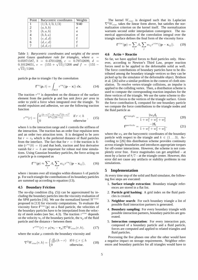
Point Barycentric coordinates Weights1 (1/3, 1/3, 1/3) 9/402 (a, b, b) e3 (b, a, b) e4 (b, b, a) e5 (c, d, d) f6 (d, c, d) f7 (d, d, c) f

Table 1: Barycentric coordinates and weights of the sevenpoint Gauss quadrature rule for triangles, where a =0.05971587, b = 0.47014206, c = 0.79742699, d =0.10128651, e = (155 +

√15)/1200 and f = (155 −√

15)/1200.

particle p due to triangle t by the convolution

fra(p, t) =∫x∈t

τ ra(|p − x|) dx. (14)

The traction τra is dependent on the distance of the surfaceelement from the particle p and has unit force per area inorder to yield a force when integrated over the triangle. Tomodel repulsion and adhesion, we use the following tractionfunction

τ ra(r) =

{k (h−r)4−(h−r0)

2(h−r)2

h2r0(2h−r0)if r < h

0 otherwise, (15)

where h is the interaction range and k controls the stiffness ofthe interaction. The traction has an order four repulsion termand an order two attraction term. It is designed to be zerofor r = r0 which is the preferred distance of fluid particlesfrom the interface. The fact that for r = 0 the traction is fi-nite (τ ra(0) = k) and that both, traction and first derivativevanish for r = h are important for robust real time simula-tions. Using Gaussian boundary particles, the force acting ona particle p is computed as

fra(p) ≈∑

i

Ai

∑j

wijτra(|p − xij |), (16)

where i iterates over all triangles within distance h of particlep. For each triangle the contributions of its boundary particlesare summed up according to equation (13).

4.5 Boundary FrictionThe no-slip condition (Eq. (5)) can be approximated by in-cluding the boundary particles into the viscosity evaluation ofthe SPH particles [16]. We use the normalized kernel W visc

proposed in [13] for viscosity computations. To evaluate theviscosity force fvisc(p) on a fluid particle, the velocities ofthe boundary particles have to be interpolated from the veloc-ity of mesh nodes (see Sec. 4.3). The traction τvisc dependson the velocity vb of the boundary particle, the vp of the fluidparticle and the distance r between them

τvisc(r) = µ(vb − vp)∇2Wvisc(r, h), (17)

where the scalar µ controls the boundary viscosity and

∇2Wvisc(r, h) ={

45πh6 (h − r) if 0 ≤ r ≤ h

0 otherwise.(18)

The kernel Wvisc is designed such that its Laplacian∇2Wvisc takes the linear form above, but satisfies the nor-malization criterion on the kernel itself. The normalizationwarrants second order interpolation convergence. The nu-merical approximation of the convolution integral over thetriangle surface defines the final form of the viscosity force

fvisc(p) =∑

i

Ai

∑j

wijτvisc(|p − xij |). (19)

4.6 Actio = ReactioSo far, we have applied forces to fluid particles only. How-ever, according to Newton’s Third Law, proper reactionforces need to be applied to the deformable solid as well.The force contributions of boundary particles have to be dis-tributed among the boundary triangle vertices so they can bepicked up by the simulator of the deformable object. Bridsonet al. [26] solve a similar problem in the context of cloth sim-ulation. To resolve vertex-triangle collisions, an impulse isapplied to the colliding vertex. Then, a distribution scheme isused to compute the corresponding reaction impulses for thethree vertices of the triangle. We use the same scheme to dis-tribute the forces to the vertices of the triangle surface. Giventhe force contribution fb computed for one boundary particlewe compute the force contributions to the triangle nodes andthe fluid particle as

f trianglek =

2wkfb1 + w2

1 + w22 + w2

3

(20)

fparticle =−2fb

1 + w21 + w2

2 + w23

, (21)

where the wk are the barycentric coordinates of the boundaryparticle with respect to the triangle and k ∈ (1 . . . 3). Ac-cording to [26] this distribution scheme provides continuityacross triangle boundaries and introduces appropriate torquesfor off-center interactions. However, the scheme is not com-pletely error free. Force magnitudes can get amplified – atmost by a factor of 8/7 – at the triangle center. However, thiserror did not cause any artifacts or stability problems in oursimulations.

5 ImplementationAt every time step of the solid and fluid simulator, the follow-ing five steps are executed:

1. Surface triangle extraction: Boundary triangle refer-ences are stored in a flat list.

2. Particle grid hashing: A grid index on the fluid parti-cles is created.

3. Neighbor search: For each boundary triangle a list ofpossible fluid interaction partners is generated.

4. Boundary sampling: For every boundary triangle withpossible interaction partners, boundary particles are gen-erated.

5. Interaction computation: For every interaction pair,composed of a boundary particle and a fluid particle,forces are computed and applied to related triangles andfluid particles.

Processing the five phases one after the other would havea negative impact on storage requirements. Neighbor refer-ences and boundary particles for all triangles would have to

5

be stored at the same time. If the computations of steps threeto five are grouped around single triangles, only data relevantfor the current triangle has to be stored at a time (Fig. 6).

... ...

Neighbor

search

Sampling

Interaction

computation

Figure 6: Algorithm overview: Triangles are processed sepa-rately. This avoids the storage of fluid particle neighbor listsand boundary particles for all triangles simultaneously.

The output of step 3 is a list, containing all fluid particleswithin interaction range h of a triangle t. To speed up thesearch for these particles we use a regular grid with spatialhashing [27]. There is a trade-off between computation timefor the neighbor search and the quality of the neighbor list.We extend the axes aligned bounding box (AABB) of t alongall axes about the interaction range. Then, we query all gridcells intersecting the extended box. We also tested tighterqueries which generate fewer neighbor candidates but theirincreased time complexity was not compensated by the re-duced cost of interaction computations.

In step 4, boundary particles are only generated for thosetriangles that have fluid particle neighbors. The boundary par-ticles for a triangle t are kept only temporarily for the inter-action computation. After t is processed, they are discarded.In this step, positions and velocities are interpolated from thetriangle nodes for each boundary particle.

To compute interaction forces in step 5 we iterate over allthe boundary particles of a triangle. For each fluid parti-cle within the interaction radius of the boundary particle, wecompute the interaction forces as described in Sec. 4 and dis-tribute them among the fluid particle and the triangle nodesaccording to Eqns. (20) and (21).

6 Results

All experiments described in this section have been per-formed on an AMD Athlon 1.8 GHz PC with 512 MB RAMand a GeForce Ti 4400 graphics card with 128 MB RAM.Note that most of the simulations are recorded in a real-timeinteractive environment. Thus, we cannot afford several sec-onds or even minutes per frame for the reconstruction andrendering of the free fluid surface as in off-line simulations[14, 15] which explains the simplistic renderings of the flu-ids.

(a) (b)

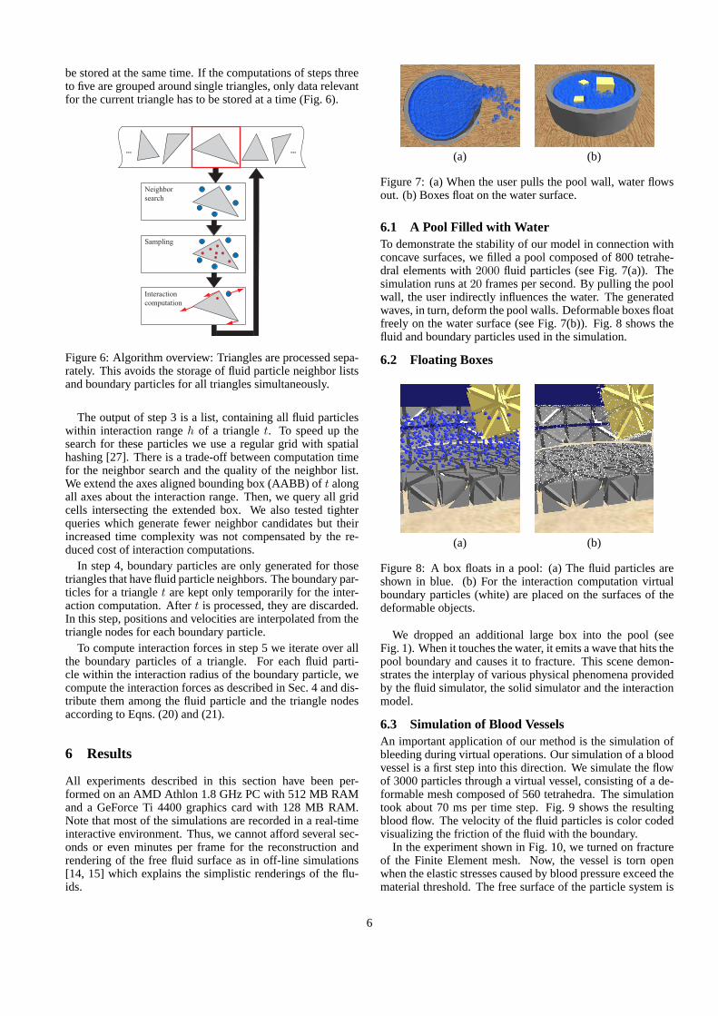
Figure 7: (a) When the user pulls the pool wall, water flowsout. (b) Boxes float on the water surface.

6.1 A Pool Filled with WaterTo demonstrate the stability of our model in connection withconcave surfaces, we filled a pool composed of 800 tetrahe-dral elements with 2000 fluid particles (see Fig. 7(a)). Thesimulation runs at 20 frames per second. By pulling the poolwall, the user indirectly influences the water. The generatedwaves, in turn, deform the pool walls. Deformable boxes floatfreely on the water surface (see Fig. 7(b)). Fig. 8 shows thefluid and boundary particles used in the simulation.

6.2 Floating Boxes

(a) (b)

Figure 8: A box floats in a pool: (a) The fluid particles areshown in blue. (b) For the interaction computation virtualboundary particles (white) are placed on the surfaces of thedeformable objects.

We dropped an additional large box into the pool (seeFig. 1). When it touches the water, it emits a wave that hits thepool boundary and causes it to fracture. This scene demon-strates the interplay of various physical phenomena providedby the fluid simulator, the solid simulator and the interactionmodel.

6.3 Simulation of Blood VesselsAn important application of our method is the simulation ofbleeding during virtual operations. Our simulation of a bloodvessel is a first step into this direction. We simulate the flowof 3000 particles through a virtual vessel, consisting of a de-formable mesh composed of 560 tetrahedra. The simulationtook about 70 ms per time step. Fig. 9 shows the resultingblood flow. The velocity of the fluid particles is color codedvisualizing the friction of the fluid with the boundary.

In the experiment shown in Fig. 10, we turned on fractureof the Finite Element mesh. Now, the vessel is torn openwhen the elastic stresses caused by blood pressure exceed thematerial threshold. The free surface of the particle system is

6

Figure 9: Blood flow through a vessel. The image shows sub-sequent time slices of an interactive animation. The velocityof the fluid particles is color coded. Yellow colored particlesare fast, while red ones are slow. Pulsation waves and viscos-ity at the vessel boundary can be observed.

Figure 10: Vessel injury. The Finite Element mesh fracturesdue to pressure forces in the blood stream.

rendered using the Marching Cubes algorithm. The anima-tion of the mesh and the particles are possible in real time at60 ms per time step, while surface reconstruction took abouthalf a second per frame. On today’s hardware only a limitednumber of fluid particles can be simulated in real-time whichyields a relatively coarse fluid surface.

7 ConclusionWe have presented a new method for the simulation of in-teractions of deformable solids with fluids. Our interactionmodel simulates repulsion, adhesion and friction near thefluid-solid interface. The smoothness of the force fields isimportant for the stability of the simulation. The core ideato get smooth interaction fields is to place boundary parti-cles onto the surface triangles according to Gauss quadraturerules. This idea might be useful in other graphic domains aswell. We mentioned the application to modeling with implicitsurfaces. Character skinning is another application wherebulges or knees are known problems in regions where severalclose bones meet.

We demonstrated the usability of our method in an interac-tive simulation environment with several scenes. A difficultyin connection with the interactive simulation of fluids is theextraction and rendering of a plausible fluid surface in realtime. Thus, ongoing work focusses on fast algorithms forsurface reconstruction.

AcknowledgementsThis project was funded by the Swiss National Commissionfor Technology and Innovation (KTI) project no. 6310.1KTS-ET.

References[1] D. Terzopoulos, J. Platt, A. Barr, and K. Fleischer. Elastically deformable models. In Computer

Graphics Proceedings, Annual Conference Series, pages 205–214. ACM SIGGRAPH 87, July1987.

[2] David Baraff and Andrew Witkin. Large steps in cloth simulation. In Proceedings of SIGGRAPH1998, pages 43–54, 1998.

[3] Mathieu Desbrun, Peter Schrder, and Alan H. Barr. Interactive animation of structured de-formable objects. In Graphics Interface ’99, 1999.

[4] Doug L. James and Dinesh K. Pai. Artdefo, accurate real time deformable objects. In ComputerGraphics Proceedings, Annual Conference Series, pages 65–72. ACM SIGGRAPH 99, August1999.

[5] Gilles Debunne, Mathieu Desbrun, Marie-Paule Cani, and Alan Barr. Dynamic real-time de-formations using space & time adaptive sampling. In Computer Graphics Proceedings, AnnualConference Series, pages 31–36. ACM SIGGRAPH 2001, August 2001.

[6] E. Grinspun, P. Krysl, and P. Schrder. CHARMS: A simple framework for adaptive simulation.In ACM Transactions on Graphics, volume 21, pages 281–290. ACM SIGGRAPH 2002, August2002.

[7] Matthias Mller, Julie Dorsey, Leonard McMillan, R. Jagnow, and B. Cutler. Stable real-timedeformations. Proceedings of 2002 ACM SIGGRAPH Symposium on Computer Animation,pages 49–54, 2002.

[8] W. T. Reeves. Particle systems — a technique for modeling a class of fuzzy objects. ACMTransactions on Graphics 2(2), pages 91–108, 1983.

[9] Mathieu Desbrun and Marie-Paule Cani. Smoothed particles: A new paradigm for animatinghighly deformable bodies. In 6th Eurographics Workshop on Computer Animation and Simula-tion ’96, pages 61–76, 1996.

[10] J.J. Monaghan. Smoothed particle hydrodynamics. Annu. Rev. Astron. Physics, 30:543, 1992.

[11] Mathieu Desbrun and Marie-Paule Cani. Space-time adaptive simulation of highly deformablesubstances. Technical report, INRIA Nr. 3829, 1999.

[12] D. Stora, P. Agliati, M. P. Cani, F. Neyret, and J. Gascuel. Animating lava flows. In GraphicsInterface, pages 203–210, 1999.

[13] Matthias Mller, David Charypar, and Markus Gross. Particle-based fluid simulation for interac-tive applications. Proceedings of 2003 ACM SIGGRAPH Symposium on Computer Animation,pages 154–159, 2003.

[14] Simon Premoze, Tolga Tasdizen, James Bigler, Aaron Lefohn, and Ross T. Whitaker. Particle-based simulation of fluids. Eurographics, 22(3):401–410, 2003.

[15] Olivier Genevaux, Arash Habibi, and Jean-Michel Dischler. Simulating fluid-solid interaction.In Graphics Interface, pages 31–38. CIPS, Canadian Human-Computer Commnication Society,A K Peters, June 2003. ISBN 1-56881-207-8, ISSN 0713-5424.

[16] J. J. Monaghan, M. Thompson, and K. Hourigan. Simulation of free surface flows with sph.ASME Symposium on Computational Methods in Fluid Dynamics, 1994.

[17] C. Pozrikidis. Numerical Computation in Science and Engineering. Oxford Univ. Press, NY,1998.

[18] T. J. Chung. Applied Continuum Mechanics. Cambridge Univ. Press, NY, 1996.

[19] J. F. O’Brien and J. K. Hodgins. Graphical modeling and animation of brittle fracture. InProceedings of SIGGRAPH 1999, pages 287–296, 1999.

[20] Jos Stam. Stable fluids. In Proceedings of the 26th annual conference on Computer graphicsand interactive techniques, pages 121–128. ACM Press/Addison-Wesley Publishing Co., 1999.

[21] N. Foster and R. Fedkiw. Practical animation of liquids. In Proceedings of the 28th annualconference on Computer graphics and interactive techniques, pages 23–30. ACM Press, 2001.

[22] D. Enright, S. Marschner, and R. Fedkiw. Animation and rendering of complex water surfaces.In Proceedings of the 29th annual conference on Computer graphics and interactive techniques,pages 736–744. ACM Press, 2002.

[23] J. Blinn. A generalization of algebraic surface drawing. ACM Transactions on Graphics,1(3):235–256, 1982.

[24] J. Bloomenthal. Skeletal Design of Natural Forms. PhD thesis, University of Calgary, Canada,1995.

[25] A. Sherstyuk. Fast ray tracing of implicit surfaces. In Implicit Sufaces ’98, pages 145–153,1998.

[26] R. Bridson, R. Fedkiw, and J. Anderson. Robust treatment of collisions, contact and frictionfor cloth animation. In ACM Transactions on Graphics, volume 21, pages 594–603. ACMSIGGRAPH 2002, August 2002.

[27] M. Teschner, B. Heidelberger, M. Mller, D. Pomeranerts, and M. Gross. Optimized spatialhashing for collision detection of deformable objects. In Proc. Vision, Modeling, VisualizationVMV, pages 47–54, 2003.

7