Interaction Effects in Multilevel Models by Gina L. Mazza A … · Interaction Effects in...

Interaction Effects in Multilevel Models

by

Gina L. Mazza

A Thesis Presented in Partial Fulfillment

of the Requirements for the Degree

Master of Arts

Approved November 2015 by the

Graduate Supervisory Committee:

Craig K. Enders, Co-Chair

Leona S. Aiken, Co-Chair

Stephen G. West

ARIZONA STATE UNIVERSITY

December 2015

i

ABSTRACT

Researchers are often interested in estimating interactions in multilevel models, but many

researchers assume that the same procedures and interpretations for interactions in single-

level models apply to multilevel models. However, estimating interactions in multilevel

models is much more complex than in single-level models. Because uncentered (RAS) or

grand mean centered (CGM) level-1 predictors in two-level models contain two sources

of variability (i.e., within-cluster variability and between-cluster variability), interactions

involving RAS or CGM level-1 predictors also contain more than one source of

variability. In this Master’s thesis, I use simulations to demonstrate that ignoring the four

sources of variability in a total level-1 interaction effect can lead to erroneous

conclusions. I explain how to parse a total level-1 interaction effect into four specific

interaction effects, derive equivalencies between CGM and centering within context

(CWC) for this model, and describe how the interpretations of the fixed effects change

under CGM and CWC. Finally, I provide an empirical example using diary data

collected from working adults with chronic pain.

ii

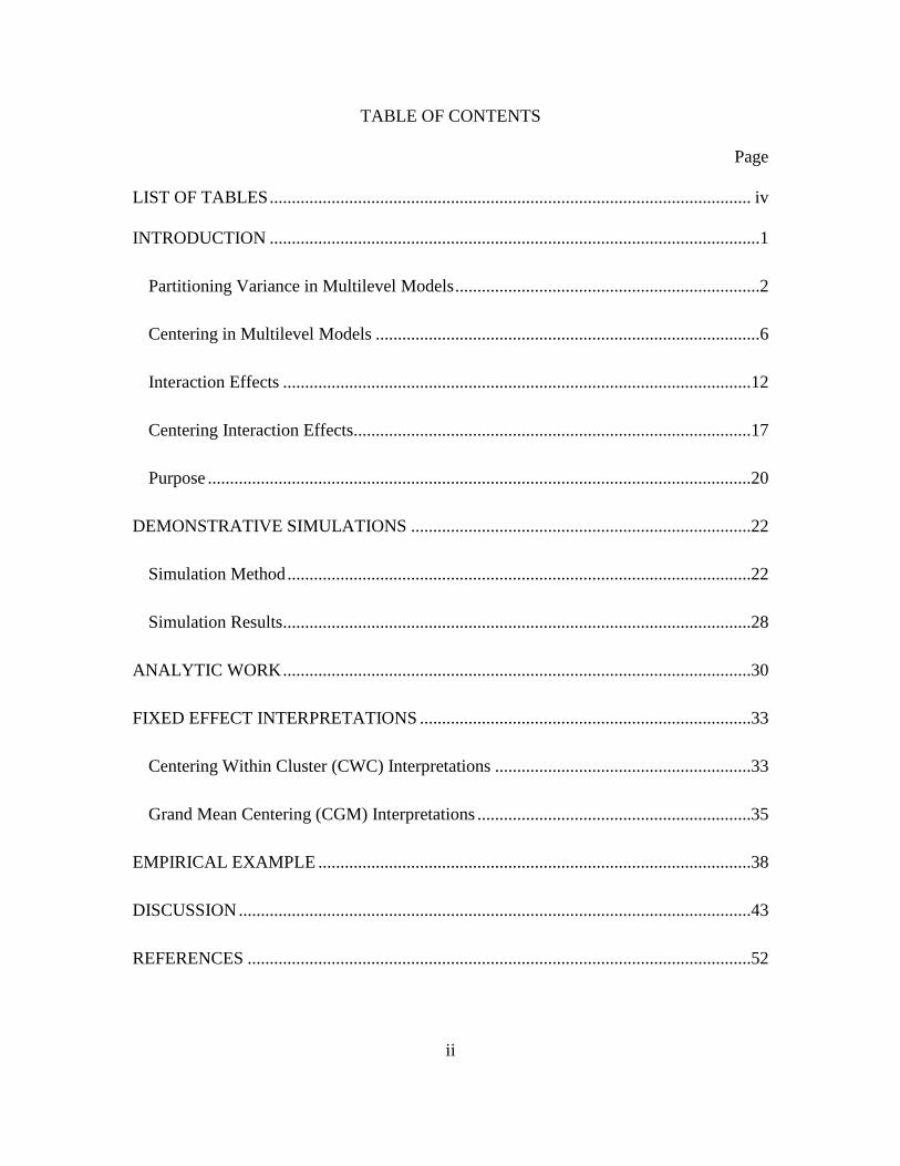
TABLE OF CONTENTS

Page

LIST OF TABLES ............................................................................................................. iv

INTRODUCTION ...............................................................................................................1

Partitioning Variance in Multilevel Models .....................................................................2

Centering in Multilevel Models .......................................................................................6

Interaction Effects ..........................................................................................................12

Centering Interaction Effects..........................................................................................17

Purpose ...........................................................................................................................20

DEMONSTRATIVE SIMULATIONS .............................................................................22

Simulation Method .........................................................................................................22

Simulation Results ..........................................................................................................28

ANALYTIC WORK ..........................................................................................................30

FIXED EFFECT INTERPRETATIONS ...........................................................................33

Centering Within Cluster (CWC) Interpretations ..........................................................33

Grand Mean Centering (CGM) Interpretations ..............................................................35

EMPIRICAL EXAMPLE ..................................................................................................38

DISCUSSION ....................................................................................................................43

REFERENCES ..................................................................................................................52

iii

Page

APPENDIX

A TABLES ....................................................................................................................57

B DERIVATIONS FROM DUNCAN, CUZZORT, AND DUNCAN (1961) .............64

C DERIVATIONS FOR DEMONSTRATIVE SIMULATIONS ................................68

D MPLUS 7.3 INPUT FILES FOR EMPIRICAL EXAMPLE ....................................71

iv

LIST OF TABLES

Table Page

1. Population Parameters by Condition .....................................................................58

2. Simulation Results by Condition ..........................................................................59

3. Sources of Variability Present in Each Term of Equation 24 with CWC or CGM

Level-1 Predictors ..................................................................................................60

4. Empirical Example, Fixed Effect Estimates with CWC Level-1 Predictors .........61

5. Empirical Example, Fixed Effect Estimates with CWC or CGM Level-1

Predictors ...............................................................................................................62

6. Pairwise Comparisons with CWC or CGM Level-1 Predictors ............................63

1

Interaction Effects in Multilevel Models

Researchers frequently collect data in which observations are clustered, or

correlated. Children are nested within families, patients are nested within healthcare

centers, employees are nested within work groups, students are nested within schools,

and repeated measures are nested within participants. Applying single-level models to

clustered data violates the independence of observations assumption of single-level

models and consequently inflates the Type I error rate. Multilevel models account for

this clustering, thus keeping the Type I error rate at the nominal significance level, and

further allow researchers to simultaneously investigate the effects of predictors at all

levels of the hierarchy.

Researchers are often interested in estimating interactions in multilevel models,

but many researchers assume that the same procedures and interpretations for interactions

in single-level models apply to multilevel models. However, estimating interactions in

multilevel models requires additional considerations not relevant to single-level models.

Because level-1 predictors in two-level models potentially have variability at both levels

of the hierarchy, interactions involving at least one level-1 predictor are composites of

two or more specific interaction effects. The purpose of this Master’s thesis is to

investigate the causes and implications of specific interaction effects embedded in total

cross-level and level-1 interaction effects, describe the impact of centering, and provide

recommendations for analyzing and interpreting total level-1 interaction effects in

multilevel models.

2

Partitioning Variance in Multilevel Models

In two-level models, we partition the outcome variable into two orthogonal

sources of variability: level-1 and level-2. Level-2 variability refers to cluster mean

differences on the outcome variable and level-1 variability refers to within-cluster

differences on the outcome variable. For example, consider a chronic pain study in

which daily observations (level 1) are nested within participants (level 2). Suppose that

the researchers are interested in predicting participants’ daily affect ratings. Level-2

variability refers to participant-to-participant differences in average affect levels (i.e.,

some participants have higher average affect levels than others), and level-1 variability

refers to day-to-day fluctuations around participants’ average affect levels (i.e.,

participants’ affect ratings may be higher or lower than their average affect levels from

day-to-day). The unconditional model with no predictors is

𝑌𝑖𝑗 = 𝛾00 + 𝑢0𝑗 + 𝜀𝑖𝑗 (1)

where 𝛾00 is the weighted grand mean, 𝑢0𝑗 is a residual that represents cluster mean

differences on the outcome variable, and 𝜀𝑖𝑗 is a residual that represents differences

between scores and their cluster-specific means. The notational system I adopt

throughout this Master’s thesis is largely consistent with that of Raudenbush and Bryk

(2002), though I use a combined form (with one equation) rather than a hierarchical form

3

(p. 35).1 In the example above, 𝛾00 is the weighted grand mean across participants, 𝑢0𝑗

represents the difference between participant j’s average affect level and the weighted

grand mean, and 𝜀𝑖𝑗 represents the difference between participant j’s affect rating on day i

and his/her average affect level. Rather than estimating the unit-specific residuals, 𝑢0𝑗

and 𝜀𝑖𝑗, we assume they are normally distributed with mean zero and estimate their

variances, 𝜎𝑢0𝑗

2 and 𝜎𝜀2, respectively.

Predictors can be measured at all levels of the hierarchy. Level-1 predictors are

measured at the lowest level of the hierarchy, level 1, whereas level-2 predictors are

measured at the next highest level of the hierarchy, level 2. Adding a level-1 predictor

𝑋𝑖𝑗 to Equation 1 yields

𝑌𝑖𝑗 = 𝛾00 + 𝛾10𝑋𝑖𝑗 + 𝑢0𝑗 + 𝜀𝑖𝑗 (2)

where 𝛾10 is the level-1 regression coefficient, 𝑢0𝑗 is a residual that represents cluster

mean differences on the outcome variable that remain after accounting for the level-1

predictor 𝑋𝑖𝑗, and 𝜀𝑖𝑗 is a residual that represents differences between scores and their

cluster-specific means that remain after accounting for the level-1 predictor 𝑋𝑖𝑗. In two-

level models, level-1 predictors potentially have two sources of variability: level-1 and

level-2. In the chronic pain study, suppose that the researchers want to predict daily

affect ratings from daily sleep ratings. Daily sleep ratings are measured at level 1 (day

1 Contrary to Raudenbush and Bryk (2002), I use 𝜀𝑖𝑗 and 𝜎𝜀

2 (rather than rij and 𝜎2) to represent the level-1

residual and its variance and I use 𝜎𝑢0𝑗2 , 𝜎𝑢1𝑗

2 , etc. (rather than τ00, τ11, etc.) to represent the level-2 (residual)

variances.

4

level), so they potentially have day-level and participant-level variability. Participant-

level variability refers to participant-to-participant differences in average sleep levels

(i.e., some participants have higher average sleep levels than others), and day-level

variability refers to day-to-day fluctuations around participants’ average sleep levels (i.e.,

participants’ sleep ratings may be higher or lower from day-to-day than their average

sleep levels).

The sources of variability in a predictor determine which associations are

estimable. Because level-1 predictors potentially have level-1 and level-2 variability,

they can have within-cluster and/or between-cluster associations with the outcome

variable. In the previous example, a within-cluster association between daily sleep

ratings and daily affect ratings means that day-to-day fluctuations around a participant’s

average sleep level predict day-to-day fluctuations around his/her average affect level. A

between-cluster association between daily sleep ratings and daily affect ratings means

that a participant’s average sleep level predicts his/her average affect level. Because we

are representing both the within-cluster and between-cluster associations with one level-1

regression coefficient 𝛾10 in Equation 2, we assume that the within-cluster and between-

cluster associations between the level-1 predictor and the outcome variable are equal. If

this assumption does not hold (i.e., there is a contextual effect), the level-1 regression

coefficient 𝛾10 is difficult to interpret (Raudenbush, 1989a; Hofmann & Gavin, 1998;

Raudenbush & Bryk, 2002). The level-1 regression coefficient 𝛾10 is actually a weighted

average of the within-cluster and between-cluster associations between the level-1

predictor and the outcome variable. Duncan, Cuzzort, and Duncan (1961) provided the

following equation:

5

𝑏𝑇 = 𝜂𝑋2 𝑏𝐵 + (1 − 𝜂𝑋

2 )𝑏𝑊 (3)

where 𝑏𝑇 is the level-1 regression coefficient (i.e., 𝛾10 in Equation 2), 𝑏𝐵 is the between-

cluster association between the level-1 predictor and the outcome variable, 𝑏𝑊 is the

within-cluster association between the level-1 predictor and the outcome variable, and 𝜂𝑋2

is the ratio of the between-cluster sum of squares on the level-1 predictor to the total sum

of squares on the level-1 predictor. The derivations corresponding to Equation 3 are

shown in Appendix B. Based on Equation 3, the level-1 regression coefficient 𝛾10 in

Equation 2 unambiguously estimates a level-specific association if (1) the within-cluster

and between-cluster associations are equal, (2) there is no variability at level 2 (i.e.,

𝜂𝑋2 = 0), or (3) there is no variability at level 1 (i.e., 𝜂𝑋

2 = 1).

Because level-2 predictors have only level-2 variability, they can have between-

cluster, but not within-cluster, associations with the outcome variable. A level-2

regression coefficient describes the between-cluster association between the level-2

predictor and the outcome variable; it is unambiguously interpreted as a between-cluster

association. For example, suppose that the researchers want to predict daily affect ratings

from history of depression. Participants report their history of depression once, not daily,

so it is measured at level 2 (participant level). A between-cluster association between

history of depression and daily affect ratings means that a participant’s history of

depression predicts his/her average affect level.

6

Centering in Multilevel Models

As in single-level models, centering can be used in multilevel models to establish

an interpretable zero point on measures that otherwise lack one (e.g., 1 to 7 Likert scale).

In single-level models, centering does not affect the regression slopes unless higher-order

effects (e.g., interaction effects, quadratic effects) are introduced (Aiken & West, 1991).

By contrast, centering often affects the parameter estimates and their interpretations in

multilevel models. Furthermore, we can use centering to isolate the associations of

interest discussed in the previous section.

Similar to the centering options for predictors in single-level models, there are

two centering options for level-2 predictors in two-level models: raw score scaling (RAS)

and grand mean centering (CGM). There are three centering options for level-1

predictors in two-level models: RAS, CGM, and centering within context (CWC; also

referred to as centering within clusters or group mean centering). This notation comes

from Kreft, de Leeuw, and Aiken (1995), which is the seminal work on centering in

multilevel models. Another centering option for level-1 or level-2 predictors is to center

scores around a meaningful constant (e.g., centering time at the first or last time point),

but I do not discuss this centering option because it has the same properties as RAS and

CGM.

RAS refers to leaving the predictor uncentered. CGM deviates scores around the

grand mean. Applying CGM to a level-1 predictor results in the following equation:

𝑋CGM = 𝑋𝑖𝑗 − �̅� (4)

7

where 𝑋𝑖𝑗 is the level-1 predictor score for case i in cluster j and �̅� is the grand mean.

Because CGM deviates scores around the same constant, it preserves level-1 and level-2

variability in the level-1 predictor. Thus, consistent with the discussion in the previous

section, level-1 predictors can have within-cluster and/or between-cluster associations

with the outcome variable after CGM. CWC is also referred to as centering within

clusters or group mean centering because it deviates scores around their cluster-specific

means. CWC results in the following equation:

𝑋CWC = 𝑋𝑖𝑗 − �̅�𝑗 (5)

where �̅�𝑗 is the mean X score in cluster j. After subtracting the cluster-specific means

from the scores, all the clusters have a mean of zero after centering. As such, there is no

variability in the cluster means of the centered sores (i.e., there is no level-2 variability)

after CWC. Thus, unlike RAS and CGM, applying CWC yields level-1 predictors with

only level-1 variability. Because level-1 predictors in two-level models have only level-1

variability after CWC, they can have within-cluster, but not between-cluster, associations

with the outcome variable. Again, consider the effect of daily sleep ratings on daily

affect ratings. CGM preserves day-level and participant-level variability in daily sleep

ratings, so it can have within-cluster and/or between-cluster associations with daily affect

ratings. After CWC, daily sleep ratings has only day-level variability, so it can have

within-cluster, but not between-cluster, associations with daily affect ratings. Thus, a

participant’s average sleep level can no longer predict his/her average affect level.

8

Much of the existing research on centering investigates centering in contextual

effect models (Blalock, 1984; Raudenbush, 1989a; Raudenbush, 1989b; Kreft et al.,

1995; Hofmann & Gavin, 1998). As noted previously, a contextual effect occurs when

the within-cluster and between-cluster associations between the level-1 predictor and the

outcome variable differ in magnitude and/or sign. For example, Simons, Wills, and Neal

(2014) collected data from 263 college students across 49 days (over a 1.3-year span) to

investigate how affective functioning influences likelihood of drinking alcohol, quantity

of alcohol consumed on drinking days, and dependence symptoms. State negative affect

(i.e., day-to-day fluctuations around participants’ average negative affect levels)

predicted higher alcohol consumption on drinking days, but trait negative affect did not

predict mean alcohol consumption on drinking days (i.e., there was a contextual effect).

As another example of a contextual effect, state negative affect did not predict likelihood

of drinking alcohol on a given day, but trait negative affect predicted a higher proportion

of drinking days (Simons, Wills, and Neals, 2014). Introducing the cluster means of the

level-1 predictor as a level-2 predictor in the model allows for a contextual effect.

Extending Equation 2 into a contextual effect model yields

𝑌𝑖𝑗 = 𝛾00 + 𝛾10𝑋𝑖𝑗 + 𝛾01�̅�𝑗 + 𝑢0𝑗 + 𝜀𝑖𝑗 (6)

where �̅�𝑗 denotes the cluster means for the level-1 predictor 𝑋𝑖𝑗 and 𝛾01 is the regression

coefficient for the cluster means.

Kreft et al. (1995) derived equivalencies and non-equivalencies between RAS,

CGM, and CWC for two models: (1) a random intercept model with one level-1 predictor

9

(i.e., Equation 2) and (2) a random intercept model with one level-1 predictor and the

cluster means to account for a contextual effect (i.e., Equation 6). Although Kreft et al.

(1995) referred to the three random intercept models as RAS1, CGM1, and CWC1 and the

three contextual effect models as RAS2, CGM2, and CWC2, here I generically use RAS,

CGM, and CWC to refer to these models. Kreft et al. (1995) defined equivalence as

having the same expectancies and dispersions (and by extension, the same model fit).

They concluded that RAS and CGM, but not CWC, are equivalent for the random

intercept model with one level-1 predictor (i.e., Equation 2).

For the random intercept model with one level-1 predictor and the cluster means

(i.e., Equation 6), RAS, CGM, and CWC are equivalent. Kreft et al. (1995) provided the

following equivalencies between CGM and CWC:

𝛾00CWC = 𝛾00

CGM − 𝛾10CGM�̅�

𝛾10CWC = 𝛾10

CGM

𝛾01CWC − 𝛾10

CWC = 𝛾01CGM

(7)

(8)

(9)

where the superscripts denote whether the parameters are CGM or CWC. Furthermore,

the residuals from Equation 6 have equivalent variances with CGM and CWC. Kreft et

al. (1995) assumed that the cluster means in Equation 6 are RAS. When the cluster

means are centered at the grand mean (as I assume here), 𝛾00CWC = 𝛾00

CGM.

However, centering changes the interpretation of the regression coefficients in

Equation 6 (Raudenbush, 1989a; Kreft et al., 1995). With RAS and CGM, the level-1

predictor 𝑋𝑖𝑗 and the cluster means �̅�𝑗 are correlated. Applying this to Equation 6, 𝛾10 is

10

a partial regression coefficient that quantifies the within-cluster association and 𝛾01 is a

partial regression coefficient that quantifies the differential influence of the cluster means

(i.e., the contextual effect). The sum of 𝛾10 and 𝛾01 equals the between-cluster

association. With CWC, the level-1 predictor 𝑋𝑖𝑗 and the cluster means �̅�𝑗 are

uncorrelated. Applying this to Equation 6, 𝛾10 quantifies the within-cluster association

and 𝛾01 quantifies the between-cluster association. The difference between 𝛾01 and 𝛾10

equals the contextual effect.

Extending Equation 6 into a random slope model yields

𝑌𝑖𝑗 = 𝛾00 + 𝛾10𝑋𝑖𝑗 + 𝛾01�̅�𝑗 + 𝑢0𝑗 + 𝑢1𝑗𝑋𝑖𝑗 + 𝜀𝑖𝑗 (10)

where 𝑢1𝑗 is a residual that allows the effect of the level-1 predictor 𝑋𝑖𝑗 to differ across

clusters. Again, rather than estimating the unit-specific residuals, 𝑢1𝑗, we assume they

are normally distributed with mean zero and estimate their variance, 𝜎𝑢1𝑗

2 .

Substantive Considerations

Kreft et al. (1995) advised researchers to choose a centering method based on

theory. Although they did not explicitly address centering, Klein, Dansereau, and Hall

(1994) agreed, saying “Too often, levels issues are considered the domain of statisticians.

We have tried to show that they are not; first and foremost, levels issues are the domain

of theorists” (p. 224). In two-level models, Klein et al. (1994) defined predictors as

either cluster-independent or cluster-dependent constructs. For cluster-independent

constructs, the interpretation of scores does not depend on other cases within the same

11

cluster. Two cases with the same raw score on the level-1 predictor would have the same

expected score on the outcome variable, regardless of cluster membership. Only a case’s

absolute standing matters. CGM is appropriate for cluster-independent constructs

because it preserves absolute score differences across clusters. For cluster-dependent

constructs, the interpretation of scores depends on other cases within the same cluster.

Two cases from different clusters could share the same raw score on the level-1 predictor

but have different expected scores on the outcome variable. A case’s standing relative to

other cases within the same cluster matters, which is commonly referred to as a frog pond

effect (Davis, 1966; Marsh & Parker, 1984). CWC is appropriate for cluster-dependent

constructs because deviations from the cluster-specific means reflect within-cluster

standing on the level-1 predictor.

For example, consider the effect of daily sleep ratings on daily affect ratings. A

cluster-independent construct definition of sleep posits that a participant’s absolute sleep

rating matters. Two participants who slept for seven hours would have the same

expected daily affect rating, regardless of how much they usually sleep. A cluster-

dependent construct definition of sleep posits that whether a participant sleeps more or

less than he/she usually does matters. Sleeping for seven hours may have a different

effect on daily affect ratings for a participant who usually sleeps for six hours than for a

participant who usually sleeps for nine hours. As another example, consider the effect of

workload on psychological well-being in a sample of employees nested within

workgroups. A cluster-independent construct definition of workload posits that an

employee’s absolute workload matters. Two employees with the same workload would

have the same expected psychological well-being, regardless of the average workload in

12

their workgroup. A cluster-dependent construct definition of workload posits that

whether an employee works more or less than the rest of his/her workgroup matters.

Working 45 hours per week may have a different effect on psychological well-being for

an employee whose workgroup works an average of 40 hours per week than for an

employee whose workgroup works an average of 50 hours per week. Thus, researchers

must decide which is more important: a case’s absolute score or score relative to its

cluster mean. Based on this decision, they should use CGM or CWC, respectively.

Interaction Effects

Psychological researchers are often interested in estimating interaction effects in

multilevel models. An informal search of American Psychological Association (APA)

journals revealed applications appearing in Health Psychology (Parsons, Rosof, &

Mustanski, 2008; Gubbels et al., 2011), Psychology of Addictive Behaviors (Patrick &

Maggs, 2009), Journal of Abnormal Psychology (Wichers et al., 2008), Journal of

Consulting and Clinical Psychology (Bryan et al., 2012; Olthuis, Watt, Mackinnon, &

Stewart, 2014; Eddington, Silvia, Foxworth, Hoet, & Kwapil, 2015), Journal of Family

Psychology (Jenkins, Dunn, O’Connor, Rasbash, & Behnke, 2005), Emotion (O’Hara,

Armeli, Boynton, & Tennen, 2014), Journal of Personality and Social Psychology

(Gleason, Iida, Shrout, & Bolger, 2008), Journal of Applied Psychology (Zohar & Luria,

2005; Bledow, Schmitt, Frese, & Kühnel, 2011), Journal of Educational Psychology (de

Boer, Bosker, & van der Werf, 2010), and Psychology and Aging (Savla et al., 2013), to

name a few. There are three types of interactions in two-level models: level-1

interactions, cross-level interactions, and level-2 interactions. A level-1 interaction is an

interaction between two level-1 predictors. For example, de Boer et al. (2010) found that

13

achievement in primary school, IQ, socioeconomic status, parents’ aspirations, and grade

repetition in primary school (level 1) moderated the effect of teacher expectation bias

(level 1) on student achievement in secondary school (level 1). A cross-level interaction

is an interaction between a level-1 predictor and a level-2 predictor. For example,

Parsons et al. (2008) found that beliefs about the importance of medication adherence

(level 2) moderated the effect of alcohol consumption (level 1) on medication adherence

(level 1) in a sample of HIV-positive men and women. Alcohol use and alcohol-related

problems (level 2) also moderated the effect of alcohol consumption (level 1) on

medication adherence (level 1). Finally, a level-2 interaction is an interaction between

two level-2 predictors. In this Master’s thesis, I focus on interactions involving level-1

predictors because analyzing level-2 interactions requires the same procedures as in

ordinary least squares (OLS) regression analysis (Aiken & West, 1991).

A cross-level interaction between a level-1 predictor 𝑋𝑖𝑗 and a level-2 predictor

𝑊𝑗 yields

𝑌𝑖𝑗 = 𝛾00 + 𝛾10𝑋𝑖𝑗 + 𝛾01𝑊𝑗 + 𝛾11𝑋𝑖𝑗𝑊𝑗 + 𝑢0𝑗 + 𝑢1𝑗𝑋𝑖𝑗 + 𝜀𝑖𝑗 (11)

where 𝛾10 is the conditional effect of the level-1 predictor 𝑋𝑖𝑗, 𝛾01 is the conditional

effect of the level-2 predictor 𝑊𝑗, 𝑋𝑖𝑗𝑊𝑗 is the product term, 𝛾11 is the regression

coefficient for the cross-level interaction, and 𝑢1𝑗 is a residual that allows the effect of

the level-1 predictor 𝑋𝑖𝑗 to differ across clusters. With RAS or CGM, a cross-level

interaction potentially yields a composite product term 𝑋𝑖𝑗𝑊𝑗 with two sources of

14

variability (Hofmann & Gavin, 1998; Enders & Tofighi, 2007; Enders, 2013). To see

these sources of variability, consider the following expansion of the cross-level

interaction in Equation 11 using CGM:

(𝑋𝑖𝑗 − �̅�)𝑊𝑗 = [(𝑋𝑖𝑗 − �̅�𝑗) + (�̅�𝑗 − �̅�)]𝑊𝑗 = (𝑋𝑖𝑗 − �̅�𝑗)𝑊𝑗 + (�̅�𝑗 − �̅�)𝑊𝑗 (12)

where (𝑋𝑖𝑗 − �̅�𝑗) is within-cluster variability in the level-1 predictor 𝑋𝑖𝑗 and (�̅�𝑗 − �̅�) is

between-cluster variability in the level-1 predictor 𝑋𝑖𝑗. As shown in Equation 12, the

product term in Equation 11 is a composite of the specific cross-level interaction

(𝑋𝑖𝑗 − �̅�𝑗)𝑊𝑗 and the specific between-cluster interaction (�̅�𝑗 − �̅�)𝑊𝑗. Here I refer to

(𝑋𝑖𝑗 − �̅�𝑗)𝑊𝑗 and (�̅�𝑗 − �̅�)𝑊𝑗 as specific interaction effects to convey that they are

embedded within (𝑋𝑖𝑗 − �̅�)𝑊𝑗 , which could be viewed as the total cross-level interaction

effect. This terminology corresponds to terminology used in the mediation and structural

equation modeling literature to discuss specific indirect effects, which comprise the total

indirect effect. In Equation 12, the specific cross-level interaction (𝑋𝑖𝑗 − �̅�𝑗)𝑊𝑗 refers to

the moderating influence of W on the within-cluster association between X and Y, and the

specific between-cluster interaction (�̅�𝑗 − �̅�)𝑊𝑗 refers to the moderating influence of W

on the between-cluster association between X and Y. Recall that a similar issue arose in

Equation 2 where the level-1 regression coefficient 𝛾10 was a weighted average of the

within-cluster and between-cluster associations between the level-1 predictor and the

outcome variable. Likewise, the regression coefficient for the total cross-level interaction

effect 𝛾11 in Equation 11 is a composite of two specific interaction effects (Hofmann &

15

Gavin, 1998). As such, Hofmann and Gavin (1998) demonstrated that a nonzero specific

between-cluster interaction can result in a significant total cross-level interaction effect,

even when no specific cross-level interaction effect exists.

The potential for specific interaction effects is even more evident with level-1

interactions. A level-1 interaction between two level-1 predictors 𝑋𝑖𝑗 and 𝑍𝑖𝑗 yields

𝑌𝑖𝑗 = 𝛾00 + 𝛾10𝑋𝑖𝑗 + 𝛾20𝑍𝑖𝑗 + 𝛾30𝑋𝑖𝑗𝑍𝑖𝑗 + 𝑢0𝑗 + 𝑢1𝑗𝑋𝑖𝑗 + 𝑢2𝑗𝑍𝑖𝑗 + 𝑢3𝑗𝑋𝑖𝑗𝑍𝑖𝑗

+ 𝜀𝑖𝑗

(13)

where 𝑋𝑖𝑗𝑍𝑖𝑗 is the product term, 𝛾30 is the regression coefficient for the level-1

interaction, 𝑢1𝑗 is a residual that allows the effect of the level-1 predictor 𝑋𝑖𝑗 to differ

across clusters, 𝑢2𝑗 is a residual that allows the effect of the level-1 predictor 𝑍𝑖𝑗 to differ

across clusters, and 𝑢3𝑗 is a residual that allows the effect of the level-1 interaction 𝑋𝑖𝑗𝑍𝑖𝑗

to differ across clusters. As before, rather than estimating the unit-specific residuals 𝑢1𝑗,

𝑢2𝑗, and 𝑢3𝑗, we assume they are normally distributed with mean zero and estimate their

variances and covariances.

Extending the logic of Equation 12, with RAS or CGM, a level-1 interaction

potentially yields a composite product term 𝑋𝑖𝑗𝑍𝑖𝑗 with four sources of variability

(Enders & Tofighi, 2007; Enders, 2013). To see the potential for specific interaction

effects, consider the following expansion of the level-1 interaction in Equation 13 using

CGM:

16

(𝑋𝑖𝑗 − �̅�)(𝑍𝑖𝑗 − �̅�) = [(𝑋𝑖𝑗 − �̅�𝑗) + (�̅�𝑗 − �̅�)][(𝑍𝑖𝑗 − �̅�𝑗) + (�̅�𝑗 − �̅�)]

= (𝑋𝑖𝑗 − �̅�𝑗)(𝑍𝑖𝑗 − �̅�𝑗) + (𝑋𝑖𝑗 − �̅�𝑗)(�̅�𝑗 − �̅�)

+ (�̅�𝑗 − �̅�)(𝑍𝑖𝑗 − �̅�𝑗) + (�̅�𝑗 − �̅�)(�̅�𝑗 − �̅�)

(14)

where (𝑍𝑖𝑗 − �̅�𝑗) is within-cluster variability in the level-1 predictor 𝑍𝑖𝑗 and (�̅�𝑗 − �̅�) is

between-cluster variability in the level-1 predictor 𝑍𝑖𝑗. As shown in Equation 14, the

product term in Equation 13 is a composite of the specific within-cluster interaction

(𝑋𝑖𝑗 − �̅�𝑗)(𝑍𝑖𝑗 − �̅�𝑗), the specific cross-level interaction (𝑋𝑖𝑗 − �̅�𝑗)(�̅�𝑗 − �̅�), the specific

cross-level interaction (�̅�𝑗 − �̅�)(𝑍𝑖𝑗 − �̅�𝑗), and the specific between-cluster interaction

(�̅�𝑗 − �̅�)(�̅�𝑗 − �̅�). The specific within-cluster interaction (𝑋𝑖𝑗 − �̅�𝑗)(𝑍𝑖𝑗 − �̅�𝑗) refers to

the moderating influence of the within-cluster portion of Z on the within-cluster

association between X and Y.2 The specific cross-level interaction (𝑋𝑖𝑗 − �̅�𝑗)(�̅�𝑗 − �̅�)

refers to the moderating influence of the between-cluster portion of Z on the within-

cluster association between X and Y. The specific cross-level interaction (�̅�𝑗 − �̅�)(𝑍𝑖𝑗 −

�̅�𝑗) refers to the moderating influence of the within-cluster portion of Z on the between-

cluster association between X and Y. Finally, the specific between-cluster interaction

(�̅�𝑗 − �̅�)(�̅�𝑗 − �̅�) refers to the moderating influence of the between-cluster portion of Z

on the between-cluster association between X and Y. Thus, 𝛾30 in Equation 13 is

2 I use the term “total level-1 interaction effect” to refer to the product of two level-1 predictors and the

term “specific within-cluster interaction effect” to refer to the first component of the total level-1

interaction effect. Similar to how a level-1 variable may contain within-cluster and/or between-cluster

variability, a total level-1 interaction effect may contain within-cluster and/or between cluster variability.

By contrast, the specific within-cluster interaction effect contains within-cluster variability but no between-

cluster variability.

17

potentially a composite of four specific interaction effects. I demonstrate this potential

for specific interaction effects later in this Master’s thesis.

Centering Interaction Effects

Recall that when we represent the association between an RAS or CGM level-1

predictor and the outcome variable with one level-1 regression coefficient (i.e., 𝛾10 in

Equation 2), we assume that the within-cluster and between-cluster associations between

the level-1 predictor and the outcome variable are equal (i.e., there is no contextual

effect). When this assumption does not hold, we can allow for a contextual effect by

introducing the cluster means of the level-1 predictor as a level-2 predictor to the model

(see Equation 6). A cross-level or level-1 interaction with unequal specific interaction

effects is analogous to a contextual effect. When we represent a cross-level interaction

with one regression coefficient (i.e., 𝛾11 in Equation 11), we assume that the specific

cross-level interaction (𝑋𝑖𝑗 − �̅�𝑗)𝑊𝑗 and the specific between-cluster interaction (�̅�𝑗 −

�̅�)𝑊𝑗 are equal. Similarly, when we represent a level-1 interaction with one regression

coefficient (i.e., 𝛾30 in Equation 13), we assume that the specific within-cluster

interaction (𝑋𝑖𝑗 − �̅�𝑗)(𝑍𝑖𝑗 − �̅�𝑗), the specific cross-level interaction (𝑋𝑖𝑗 − �̅�𝑗)(�̅�𝑗 − �̅�),

the specific cross-level interaction (�̅�𝑗 − �̅�)(𝑍𝑖𝑗 − �̅�𝑗), and the specific between-cluster

interaction (�̅�𝑗 − �̅�)(�̅�𝑗 − �̅�) are equal. As with contextual effects, we can address

specific interaction effects by centering and/or including additional product terms in the

model.

Raudenbush (1989a, 1989b) and Hofmann and Gavin (1998) recommended

applying CWC to the level-1 predictor when estimating a cross-level interaction to

18

remove the specific between-cluster interaction. Recall that level-1 predictors do not

have level-2 variability after CWC, so (�̅�𝑗 − �̅�) = 0 in Equations 12 and 14 and (�̅�𝑗 −

�̅�) = 0 in Equation 14. As such, Equation 12 reduces to (𝑋𝑖𝑗 − �̅�𝑗)𝑊𝑗 and Equation 14

reduces to (𝑋𝑖𝑗 − �̅�𝑗)(𝑍𝑖𝑗 − �̅�𝑗) when the level-1 predictors are centered at the cluster

means. Thus, 𝛾11 in Equation 11 only reflects the specific cross-level interaction

(𝑋𝑖𝑗 − �̅�𝑗)𝑊𝑗 and 𝛾30 in Equation 13 only reflects the specific within-cluster interaction

(𝑋𝑖𝑗 − �̅�𝑗)(𝑍𝑖𝑗 − �̅�𝑗). This strategy presumes that the research question requires a frog

pond effect and that the other specific interaction effects are not of interest. When the

latter presumption does not hold, Raudenbush (1989a, 1989b) and Hofmann and Gavin

(1998) recommended using the following equation to allow for a contextual effect and a

between-cluster interaction:

𝑌𝑖𝑗 = 𝛾00 + 𝛾10(𝑋𝑖𝑗 − �̅�𝑗) + 𝛾01�̅�𝑗 + 𝛾02𝑊𝑗 + 𝛾03�̅�𝑗𝑊𝑗 + 𝛾11(𝑋𝑖𝑗 − �̅�𝑗)𝑊𝑗

+ 𝑢0𝑗 + 𝑢1𝑗𝑋𝑖𝑗 + 𝜀𝑖𝑗

(15)

where 𝛾03 is the regression coefficient for the specific between-cluster interaction effect

and 𝛾11 is the regression coefficient for the specific cross-level interaction effect.

Estimating the specific interaction effects with Equation 15 is analogous to addressing a

contextual effect with Equation 6. Including the second product term in Equation 15

allows the specific cross-level interaction effect (𝑋𝑖𝑗 − �̅�𝑗)𝑊𝑗 and the specific between-

cluster interaction effect (�̅�𝑗 − �̅�)𝑊𝑗 to differ.

19

Recall that we could use either CGM or CWC for the contextual effect model in

Equation 6 because they are equivalent. Similarly, Enders and Tofighi (2007)

generalized Equation 15 so that we can apply CGM or CWC to the level-1 predictor 𝑋𝑖𝑗:

𝑌𝑖𝑗 = 𝛾00 + 𝛾10𝑋𝑖𝑗 + 𝛾01�̅�𝑗 + 𝛾02𝑊𝑗 + 𝛾03�̅�𝑗𝑊𝑗 + 𝛾11𝑋𝑖𝑗𝑊𝑗 + 𝑢0𝑗 + 𝑢1𝑗𝑋𝑖𝑗

+ 𝜀𝑖𝑗 . (16)

Enders and Tofighi (2007) demonstrated that CGM and CWC provide equivalent fixed

effects as follows:

𝛾00CWC = 𝛾00



CWC = 𝛾01CGM

𝛾02CWC = 𝛾02



CWC = 𝛾03CGM

𝛾10CWC = 𝛾10

CGM

𝛾11CWC = 𝛾11

CGM.

(17)

(18)

(19)

(20)

(21)

(22)

As with the contextual effect model in Equation 6, centering changes the interpretation of

the regression coefficients in Equation 16 (Enders & Tofighi, 2007). Because 𝑋𝑖𝑗 and �̅�𝑗

are correlated when we apply CGM, 𝛾11 quantifies the specific cross-level interaction

effect and 𝛾03 quantifies the differential influence of the specific between-cluster

interaction effect (i.e., the additional moderating effect of the level-2 variable on the

20

level-1 variable’s cluster means). Because 𝑋𝑖𝑗 and �̅�𝑗 are uncorrelated when we apply

CWC, 𝛾11 quantifies the specific cross-level interaction effect and 𝛾03 quantifies the

specific between-cluster interaction effect. These types of equivalencies between CGM

and CWC have not been examined for level-1 interactions. Deriving these equivalencies

is one of the goals of this Master’s thesis.

Purpose

As noted previously, researchers across many fields of psychology have examined

interaction effects in multilevel models (e.g., Parsons et al., 2008; Gubbels et al., 2011;

Patrick & Maggs, 2009; Wichers et al., 2008; Bryan et al., 2012; Olthuis et al., 2014;

Eddington et al., 2015; Jenkins et al., 2005; O’Hara et al., 2014; Gleason et al., 2008;

Zohar & Luria, 2005; Bledow et al., 2011; de Boer et al., 2010; Savla et al., 2013). Such

widespread interest warrants further research on estimating and interpreting moderation

effects in multilevel models. Cronbach and Webb first raised the impact of centering on

cross-level interactions in 1975, and since then, methodologists have provided further

recommendations for estimating and interpreting cross-level interactions while applying

either CWC or CGM to the level-1 predictor (Hofmann & Gavin, 1998; Enders &

Tofighi, 2007). Although Raudenbush (1989b), Hofmann and Gavin (1998), and Enders

and Tofighi (2007) described how to use two product terms to investigate the specific

cross-level interaction effect and the specific between-cluster interaction effect, my

informal review of APA journals suggests that using one product term to represent a

cross-level interaction is the norm. Some researchers applied RAS or CGM to the level-1

predictor (e.g., Parsons et al., 2008), but I predominantly found examples of researchers

applying CWC (e.g., Bledow et al., 2011; O’Hara et al., 2014; Patrick & Maggs, 2009).

21

Although group mean centering the level-1 predictor may be justifiable based on theory,

researchers should be aware that doing so is not necessary.3

Similarly, when providing recommendations for probing cross-level interactions,

methodologists used a model consistent with Equation 11, which contains one product

term (Tate, 2004; Bauer & Curran, 2005; Curran, Bauer, & Willoughby, 2006; Preacher,

Curran, & Bauer, 2006). If the level-1 predictor involved in the cross-level interaction is

uncentered or grand mean centered (e.g., empirical example starting on page 81 of Tate,

2004; cross-level interaction between student-level aptitude and school-level consistency

with statewide recommended curriculum objectives, which are both grand mean

centered), using one product term assumes that the specific cross-level interaction effect

and specific between-cluster interaction effect are equal in magnitude and sign and can

thus be adequately represented by one regression coefficient (𝛾11 in Equation 11). If the

level-1 predictor involved in the cross-level interaction is group mean centered (e.g.,

empirical example starting on page 392 of Bauer & Curran, 2005; cross-level interaction

between student-level socioeconomic status, which was group mean centered, and school

sector), using one product term assumes that the research question requires a frog pond

effect and that the specific between-cluster interaction effect is not of interest. In this

Master’s thesis, I urge researchers to be more cognizant of the sources of variability

present in cross-level and level-1 interactions. Readers should refer to Enders and

3 For example, Aguinis et al. (2013) stated that “Enders and Tofighi (2007) argued that if a researcher uses

[CGM] for the [level-1] predictor, it is not possible to make an accurate, or even meaningful, interpretation

of the cross-level interaction” (p. 1512). Enders and Tofighi (2007) argued the opposite; they stated that

both CWC and CGM can be used to appropriately distinguish between the specific interaction effects

embedded in a total cross-level or level-1 interaction effect.

22

Tofighi (2007) for recommendations on estimating cross-level interactions while

applying either CGM or CWC to the level-1 predictor.

For this Master’s thesis, I focus on level-1 interactions. In his multilevel

modeling chapter in the APA Handbook of Research Methods in Psychology, Nezlek

(2012) noted that level-1 interactions have received very little attention in the

methodological literature. As such, the goals of this Master’s thesis are to use

simulations to demonstrate why researchers should be aware of the four sources of

variability present in a level-1 interaction, investigate equivalencies across CGM and

CWC, explain how centering affects the fixed effect interpretations, and provide

recommendations to researchers interested in estimating level-1 interactions in two-level

models.

The organization of this Master’s thesis is as follows. First I use simulations to

demonstrate that ignoring the four sources of variability in a level-1 interaction can lead

to erroneous conclusions. Next I derive equivalencies between CGM and CWC for a

model that uses four product terms to represent the specific interaction effects. I then

describe how the interpretations of the fixed effects change under these two centering

methods. Finally, I provide an empirical example using diary data collected from

working adults with chronic pain.

Simulation Method

Hofmann and Gavin (1998) used simulations to demonstrate that a nonzero

specific between-cluster interaction effect can result in a significant total cross-level

interaction effect, even when no specific cross-level interaction effect exists. To extend

this work, I performed simulations to demonstrate that a nonzero specific between-cluster

23

interaction effect or nonzero specific cross-level interaction effect(s) can result in a

significant total level-1 interaction effect, even when no specific within-cluster

interaction effect exists. These simulations, while demonstrating a predictable

phenomenon, emphasize the importance of considering and testing for specific

interaction effects, particularly when substantive theory is vague with regard to level

issues. Although it is unclear how often these configurations of specific interaction

effects might occur in practice, the simulation results indicate that researchers may be

misinterpreting total level-1 interaction effects.

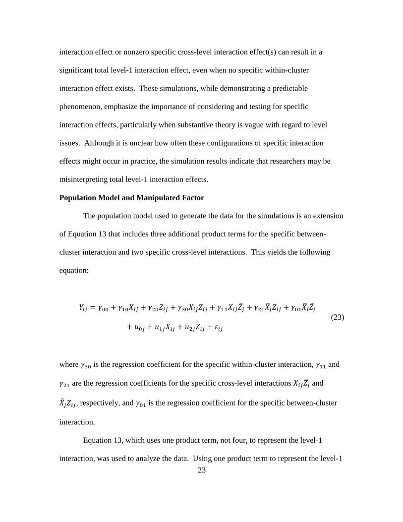
Population Model and Manipulated Factor

The population model used to generate the data for the simulations is an extension

of Equation 13 that includes three additional product terms for the specific between-

cluster interaction and two specific cross-level interactions. This yields the following

equation:

𝑌𝑖𝑗 = 𝛾00 + 𝛾10𝑋𝑖𝑗 + 𝛾20𝑍𝑖𝑗 + 𝛾30𝑋𝑖𝑗𝑍𝑖𝑗 + 𝛾11𝑋𝑖𝑗�̅�𝑗 + 𝛾21�̅�𝑗𝑍𝑖𝑗 + 𝛾01�̅�𝑗�̅�𝑗

+ 𝑢0𝑗 + 𝑢1𝑗𝑋𝑖𝑗 + 𝑢2𝑗𝑍𝑖𝑗 + 𝜀𝑖𝑗

(23)

where 𝛾30 is the regression coefficient for the specific within-cluster interaction, 𝛾11 and

𝛾21 are the regression coefficients for the specific cross-level interactions 𝑋𝑖𝑗�̅�𝑗 and

�̅�𝑗𝑍𝑖𝑗, respectively, and 𝛾01 is the regression coefficient for the specific between-cluster

interaction.

Equation 13, which uses one product term, not four, to represent the level-1

interaction, was used to analyze the data. Using one product term to represent the level-1

24

interaction is consistent with what researchers apply in practice; through my informal

review of APA journals, I found no examples that used more than one product term to

represent a level-1 interaction. Recall that this product term is a composite of four

sources of variability; further recall that the sign and magnitude of these specific

interaction effects need not be the same (see Equation 14). To demonstrate that 𝛾30 in

Equation 13 could be significant due to a nonzero specific within-cluster interaction

effect, nonzero specific cross-level interaction effect(s), and/or nonzero specific between-

cluster interaction effect, I set these four specific interactions to be nonzero one at a time

and looked at the proportion of replications where 𝛾30 was significant. Thus, there were

five conditions: (1) the specific within-cluster interaction effect was nonzero but the other

specific interaction effects equaled zero, (2) the specific cross-level interaction effect

𝑋𝑖𝑗�̅�𝑗 was nonzero but the other specific interaction effects equaled zero, (3) the specific

cross-level interaction effect �̅�𝑗𝑍𝑖𝑗 was nonzero but the other specific interaction effects

equaled zero, (4) the specific between-cluster interaction effect was nonzero but the other

specific interaction effects equaled zero, and (5) all of the specific interaction effects

equaled zero. Condition (5) was included to test the Type I error rate, which was set to

α = .05. The specific within-cluster interaction in condition (1) explained 16% of the

level-1 variance 𝜎𝜀2, the specific cross-level interaction 𝑋𝑖𝑗�̅�𝑗 in condition (2) explained

16% of the level-1 predictor 𝑋𝑖𝑗’s slope variance 𝜎𝑢1𝑗

2 , the specific cross-level interaction

�̅�𝑗𝑍𝑖𝑗 in condition (3) explained 16% of the level-1 predictor 𝑍𝑖𝑗’s slope variance 𝜎𝑢2𝑗

2 ,

and the specific between-cluster interaction in condition (4) explained 16% of the

variance in the level-2 intercept variance 𝜎𝑢0𝑗

2 . The equations used to derive the

25

population parameters that corresponded to 16% of the variance explained in each

condition are in Appendix C. The population parameters for each condition are

summarized in Table 1.

Data Generation

I used the IML procedure in SAS 9.4 to generate 2000 data sets within each of the

five conditions. I generated data for a balanced design with 50 clusters and 20 level-1

units per cluster. Such a design could arise from diary data with 50 participants and

intensive measurements (i.e., 20 observations per participant). I set the number of

clusters to 50 because Kreft and de Leeuw (1998) suggested that multilevel modeling

requires 30 clusters at minimum, and Maas and Hox (2005) stated that collecting data

from 50 clusters is typical in educational and organizational research. Maas and Hox

(2005) also stated that a cluster size of 30 is typical in educational research, but smaller

cluster sizes are typical in other fields of research. Thus, I set the cluster size to 20,

which is consistent with the empirical example described later in this Master’s thesis in

which participants provided diary data across 21 days. Based on an unconditional model

with no predictors, the level-1 variance 𝜎𝜀2 and the level-2 intercept variance 𝜎𝑢0𝑗

2 were

each set to 1. Thus, I assumed that 50% of the variability in the outcome variable was at

level 2, which corresponds to an intraclass correlation (ICC) of .5. This ICC is about

what we would expect when repeated measures are nested within participants (Spybrook,

Bloom, Congdon, Hill, Martinez, & Raudenbush, 2011). As shown in Table 1, the grand

means of the level-1 predictors 𝑋𝑖𝑗 and 𝑍𝑖𝑗 were set to zero and the covariance was set to

zero. Generating uncorrelated level-1 predictors minimized the correlations among the

four product terms, which aided in isolating the impact of each specific interaction effect.

26

However, readers should note that the simulation conditions represent a special case,

limiting the generalizability of the results. Because the level-1 predictors were generated

to be normally distributed, the mean of the product term for the level-1 interaction

equaled zero and the variance equaled 1.

To generate data for 𝑋𝑖𝑗 within each cluster, I randomly drew 20 values from a

standard normal distribution and then subtracted the mean of these 20 values. Only

within-cluster variability remained after deviating scores around their cluster-specific

means (i.e., applying CWC). Next I randomly drew 50 values from a standard normal

distribution to represent the 50 cluster means. I used the same procedure to generate data

for 𝑍𝑖𝑗. I formed the specific within-cluster interaction by multiplying the within-cluster

portions of X and Z, the specific cross-level interaction 𝑋𝑖𝑗�̅�𝑗 by multiplying the within-

cluster portion of X and the between-cluster portion of Z, the specific within-cluster

interaction �̅�𝑗𝑍𝑖𝑗 by multiplying the between-cluster portion of X and the within-cluster

portion of Z, and the specific between-cluster interaction by multiplying the between-

cluster portions of X and Z. Data for 𝑌𝑖𝑗 were generated according to Equation 23 by

substituting the aforementioned scores and the regression coefficients from Table 1. The

level-2 residuals 𝑢0𝑗, 𝑢1𝑗, and 𝑢2𝑗 in Equation 23 were generated by creating a 50-by-3

matrix whose elements were randomly drawn from a standard normal distribution and

then multiplying it by the level-2 residual covariance matrix; for each condition, the

level-2 residual covariance matrix was specified according to the values reported in Table

1. The level-1 residual 𝜀𝑖𝑗 in Equation 23 was randomly drawn from a standard normal

distribution. The simulation script is available upon request.

27

Analysis and Outcomes

All analyses were performed using the MIXED procedure in SAS 9.4. The data

from each condition and replication were analyzed according to Equation 13 using

restricted maximum likelihood estimation. The covariance matrix for the random effects

was specified as unstructured. Recall that the analysis model (Equation 13) only included

one product term, 𝑋𝑖𝑗𝑍𝑖𝑗. The regression coefficient attached to this product term—

𝛾30—was of primary interest. Within each design cell, I examined the number of

converged solutions, mean estimate of 𝛾30 across the 2000 replications, and percentage of

replications that 𝛾30 was significantly different from zero. 𝛾30 was deemed significant if

the p-value for a two-tailed t-test using Satterthwaite degrees of freedom was less than or

equal to the nominal significance level of α = .05.

For these simulations (and for the empirical example described later in this

Master’s thesis), I used what Lüdtke, Marsh, Robitzsch, and Trautwein (2011) referred to

as a doubly manifest approach, which assumes no sampling or measurement error.

Lüdtke et al. (2008) and Lüdtke et al. (2011) showed that the doubly manifest approach

(referred to as the multilevel manifest covariate approach in Lüdtke et al., 2008) can

provide biased contextual effect estimates and standard errors. For contextual effect

models, Lüdtke et al. (2008) and Lüdtke et al. (2011) proposed latent covariate

approaches that correct for sampling and/or measurement error. However, generalizing

these latent covariate approaches to other models and testing their performance is beyond

the scope of this Master’s thesis.4 These simulations serve to demonstrate that any one

4 Using the observed cluster means may not lead to substantial bias in the demonstrative simulations due to

the very high ICC and relatively large cluster size. If we view the cluster means as reflective aggregations

of level-1 constructs (i.e., members of a cluster rate a level-2 construct and, ideally, each member would

28

nonzero specific interaction can result in a significant total level-1 interaction effect—a

property that would hold regardless of whether we correct for sampling and/or

measurement error.

Simulation Results

The number of converged solutions, mean estimate of 𝛾30, and percentage of

significant 𝛾30 by condition are reported in Table 2. When all of the specific interaction

effects equaled zero, the mean estimate of 𝛾30 was -0.002. 𝛾30 was significant in 5.76%

of the data sets, which is close to the nominal significance level of α = .05.

When the specific within-cluster interaction effect was nonzero but the other

specific interactions equaled zero, the mean estimate of 𝛾30 was 0.268. However, the

population parameter for the specific within-cluster interaction effect was 0.400. As

discussed earlier, the total level-1 interaction effect is a composite of a specific within-

cluster interaction effect, two specific cross-level interaction effects, and a specific

between-cluster interaction effect. Because the two specific cross-level interaction

effects and the specific between-cluster interaction effect equaled zero in this condition,

𝛾30 is a weighted average of 0.400, 0, 0, and 0. As such, the level-1 interaction may not

be significant, even when a specific within-cluster interaction effect exists. Despite this

attenuation, when the specific within-cluster interaction effect was nonzero but the other

interactions equaled zero, 𝛾30 was significant in 99.95% of the data sets.

assign the same rating; Lüdtke et al., 2008), we can estimate the reliability of the cluster means using the

following formula from Snijders and Bosker (2012):

L2 Reliability(�̅�𝑗) =𝑛𝑗 ∙ ICC

1 + (𝑛𝑗 − 1) ∙ ICC

where nj denotes the cluster size and ICC represents the reliability of a single member’s rating. Notice that

the formula above is the Spearman-Brown formula. Substituting the ICC (.5) and cluster size (20) from the

simulated data yields a reliability of .9524.

29

When the specific cross-level interaction effect 𝑋𝑖𝑗�̅�𝑗 was nonzero but the other

specific interactions equaled zero, the mean estimate of 𝛾30 was 0.048. However, the

population parameter for the specific cross-level interaction effect 𝑋𝑖𝑗�̅�𝑗 was 0.219.

Because the specific within-cluster interaction effect, the specific cross-level interaction

effect �̅�𝑗𝑍𝑖𝑗, and the specific between-cluster interaction effect equaled zero in this

condition, 𝛾30 is a weighted average of 0, 0.400, 0, and 0. When the specific cross-level

interaction effect 𝑋𝑖𝑗�̅�𝑗 was nonzero but the other specific interactions equaled zero, 𝛾30

was significant in 19.42% of the data sets. Similarly, when the specific cross-level

interaction effect �̅�𝑗𝑍𝑖𝑗 was nonzero but the other specific interactions equaled zero, the

mean estimate of 𝛾30 was 0.049 and 𝛾30 was significant in 19.97% of the data sets.

When the specific between-cluster interaction effect was nonzero but the other

specific interactions equaled zero, the mean estimate of 𝛾30 was -0.029. However, the

population parameter for the specific between-cluster interaction effect was 0.400.

Because the specific within-cluster interaction effect and the two specific cross-level

interaction effects equaled zero in this condition, 𝛾30 is a weighted average of 0, 0, 0, and

0.400. When the specific between-cluster interaction effect was nonzero but the other

specific interactions equaled zero, 𝛾30 was significant in 10.47% of the data sets. The

results of this simulation study demonstrate that 𝛾30 in Equation 13 could be significant

due to a nonzero specific within-cluster interaction effect, nonzero specific cross-level

interaction effect(s), and/or nonzero specific between-cluster interaction effect. Again,

although it is unclear how often these configurations of specific interaction effects might

occur in practice, the simulation results demonstrate that failing to test for specific

30

interaction effects can lead to erroneous conclusions about a total level-1 interaction

effect.

Analytic Work

Although Enders and Tofighi (2007) established the equivalence of CGM and

CWC in models that address the two sources of variability in a total cross-level

interaction effect, this work has not been extended to total level-1 interaction effects

because currently no models exist for addressing the four sources of variability. I

propose estimating a model that includes the cluster means for the level-1 predictors and

three additional product terms for the specific between-cluster interaction effect and two

specific cross-level interaction effects. This yields the following equation, which is an

extension of Equation 23 that includes the cluster means for the level-1 predictors:

𝑌𝑖𝑗 = 𝛾00 + 𝛾10𝑋𝑖𝑗 + 𝛾20𝑍𝑖𝑗 + 𝛾01�̅�𝑗 + 𝛾02�̅�𝑗 + 𝛾30𝑋𝑖𝑗𝑍𝑖𝑗 + 𝛾11𝑋𝑖𝑗�̅�𝑗 +

𝛾21�̅�𝑗𝑍𝑖𝑗 + 𝛾03�̅�𝑗�̅�𝑗 + [random effects]. (24)

In Equation 24, 𝑋𝑖𝑗𝑍𝑖𝑗 represents the specific within-cluster interaction, 𝑋𝑖𝑗�̅�𝑗 and �̅�𝑗𝑍𝑖𝑗

represent the specific cross-level interactions, and �̅�𝑗�̅�𝑗 represents the specific between-

cluster interaction. Using four product terms allows us to parse the total level-1

interaction effect into its four specific interaction effects. Either CGM or CWC may be

applied to the two level-1 predictors, 𝑋𝑖𝑗 and 𝑍𝑖𝑗, in Equation 24. As such, the purpose of

this section is to explore equivalencies across the two centering methods and ultimately

understand how to interpret the fixed effects under CGM and CWC.

31

I investigated whether the fixed effects in Equation 24 are equivalent under CGM

and CWC by following the procedure used in Kreft et al. (1995) and in Enders and

Tofighi (2007). The CGM and CWC fixed effects are equivalent if the following

equation is true:

𝛾00CGM + 𝛾10

CGM(𝑋𝑖𝑗 − �̅�) + 𝛾20CGM(𝑍𝑖𝑗 − �̅�) + 𝛾01

CGM�̅�𝑗 + 𝛾02CGM�̅�𝑗

+ 𝛾30CGM(𝑋𝑖𝑗 − �̅�)(𝑍𝑖𝑗 − �̅�) + 𝛾11

CGM(𝑋𝑖𝑗 − �̅�)�̅�𝑗

+ 𝛾21CGM�̅�𝑗(𝑍𝑖𝑗 − �̅�) + 𝛾03

CGM�̅�𝑗�̅�𝑗

= 𝛾00CWC + 𝛾10

CWC(𝑋𝑖𝑗 − �̅�𝑗) + 𝛾20CWC(𝑍𝑖𝑗 − �̅�𝑗) + 𝛾01

CWC�̅�𝑗 + 𝛾02CWC�̅�𝑗 +

𝛾30CWC(𝑋𝑖𝑗 − �̅�𝑗)(𝑍𝑖𝑗 − �̅�𝑗) + 𝛾11

CWC(𝑋𝑖𝑗 − �̅�𝑗)�̅�𝑗 + 𝛾21CWC�̅�𝑗(𝑍𝑖𝑗 − �̅�𝑗) +

𝛾03CWC�̅�𝑗�̅�𝑗.

(25)

Equation 25 can be further expanded as follows:

𝛾00CGM + 𝛾10

CGM𝑋𝑖𝑗 − 𝛾10CGM�̅� + 𝛾20

CGM𝑍𝑖𝑗 − 𝛾20CGM�̅� + 𝛾01

CGM�̅�𝑗 + 𝛾02CGM�̅�𝑗

+ 𝛾30CGM𝑋𝑖𝑗𝑍𝑖𝑗 − 𝛾30

CGM𝑋𝑖𝑗�̅� − 𝛾30CGM�̅�𝑍𝑖𝑗 + 𝛾30

CGM�̅��̅�

+ 𝛾11CGM𝑋𝑖𝑗�̅�𝑗 − 𝛾11

CGM�̅��̅�𝑗 + 𝛾21CGM�̅�𝑗𝑍𝑖𝑗 − 𝛾21

CGM�̅�𝑗�̅� + 𝛾03CGM�̅�𝑗�̅�𝑗

= 𝛾00CWC + 𝛾10

CWC𝑋𝑖𝑗 − 𝛾10CWC�̅�𝑗 + 𝛾20

CWC𝑍𝑖𝑗 − 𝛾20CWC�̅�𝑗 + 𝛾01

CWC�̅�𝑗 + 𝛾02CWC�̅�𝑗

+ 𝛾30CWC𝑋𝑖𝑗𝑍𝑖𝑗 − 𝛾30

CWC𝑋𝑖𝑗�̅�𝑗 − 𝛾30CWC�̅�𝑗𝑍𝑖𝑗 + 𝛾30

CWC�̅�𝑗�̅�𝑗

+ 𝛾11CWC𝑋𝑖𝑗�̅�𝑗 − 𝛾11

CWC�̅�𝑗�̅�𝑗 + 𝛾21CWC�̅�𝑗𝑍𝑖𝑗 − 𝛾21

CWC�̅�𝑗�̅�𝑗

+ 𝛾03CWC�̅�𝑗�̅�𝑗

(26)

32

Next I collected like terms from both sides of Equation 26. Like terms refers to terms

that contain the same variable raised to the same power. Equation 26 has nine sets of like

terms: constants (including �̅� and �̅�), terms containing 𝑋𝑖𝑗 (only, e.g., not 𝑋𝑖𝑗�̅�𝑗), terms

containing 𝑍𝑖𝑗, terms containing �̅�𝑗, terms containing �̅�𝑗, terms containing 𝑋𝑖𝑗𝑍𝑖𝑗, terms

containing 𝑋𝑖𝑗�̅�𝑗, terms containing �̅�𝑗𝑍𝑖𝑗, and terms containing �̅�𝑗�̅�𝑗 . Collecting like

terms from both sides of Equation 26 yields the following solution:

𝛾00CGM − 𝛾10

CGM�̅� − 𝛾20CGM�̅� + 𝛾30

CGM�̅��̅� = 𝛾00CWC


CGM�̅� = 𝛾10CWC


CGM�̅� = 𝛾20CWC


CGM�̅� = 𝛾01CWC − 𝛾10

CWC or (𝛾10CGM − 𝛾30

CGM�̅�) + (𝛾01CGM − 𝛾21

CGM�̅�) = 𝛾01CWC


CGM�̅� = 𝛾02CWC − 𝛾20

CWC or (𝛾20CGM − 𝛾30

CGM�̅�) + (𝛾02CGM − 𝛾11

CGM�̅�) = 𝛾02CWC

𝛾30CGM = 𝛾30

CWC

𝛾11CGM = 𝛾11

CWC − 𝛾30CWC or 𝛾11

CGM + 𝛾30CGM = 𝛾11

CWC

𝛾21CGM = 𝛾21



CWC

𝛾03CGM = 𝛾03

CWC + 𝛾30CWC − 𝛾11


CGM + 𝛾11CGM + 𝛾21


CWC.

(27)

(28)

(29)

(30)

(31)

(32)

(33)

(34)

(35)

Thus, the fixed effects in Equation 24 are equivalent under CGM and CWC. When 𝑋𝑖𝑗

and 𝑍𝑖𝑗 are either CWC or CGM and the cluster means are centered at the grand mean,

Equations 27 to 31 simplify as follows:

𝛾00CGM = 𝛾00

CWC (36)

33

𝛾10CGM = 𝛾10

CWC

𝛾20CGM = 𝛾20

CWC

𝛾01CGM = 𝛾01



CWC

𝛾02CGM = 𝛾02



CWC.

(37)

(38)

(39)

(40)

Centering the cluster means does not affect Equations 32 to 35.

Fixed Effect Interpretations

The simulation results demonstrate that any one nonzero specific interaction

effect can result in a significant total level-1 interaction effect. As such, I show how to

parse a total level-1 interaction effect into its four components using Equation 24. The

analytic work in the previous section shows that Equation 24 provides equivalent fixed

effects under CWC and CGM. In this section, I provide interpretations for the fixed

effects in Equation 24 when CWC is applied to the level-1 predictors and when CGM is

applied to the level-1 predictors; in both cases I assume that the cluster means are grand

mean centered. As noted previously, the specific interaction effects are analogous to

contextual effects. Kreft et al. (1995) explained that the fixed effect interpretations for a

contextual effect model differ under CWC and CGM. Similarly, the fixed effect

interpretations for Equation 24 differ under these two centering methods, as I discuss

below.

CWC Interpretations

Interpreting the fixed effects in Equation 24 is easier with CWC than with CGM

because CWC partitions each level-1 predictor into two orthogonal sources of variability:

within-cluster variability and between-cluster variability. Table 3 summarizes the

34

sources of variability present in each term of Equation 24 under CWC and CGM. Recall

that CWC removes between-cluster variability from a level-1 predictor because all the

clusters have a mean of zero after centering. As such, Table 3 shows that fewer terms in

Equation 24 contain between-cluster variability with CWC than with CGM. Returning to

Equation 24, 𝛾00CWC is the expected value of 𝑌𝑖𝑗 for a case that is average relative to the

other cases in its cluster and from a cluster that is average relative to the other clusters on

both level-1 predictors. 𝛾10CWC is the conditional within-cluster effect of 𝑋𝑖𝑗 for a case that

is average relative to the other cases in its cluster and from a cluster that is average

relative to the other clusters on Z (𝑍𝑖𝑗 = 0 and �̅�𝑗 = 0). Similarly, 𝛾20CWC is the

conditional within-cluster effect of 𝑍𝑖𝑗 for a case that is average relative to the other cases

in its cluster and from a cluster that is average relative to the other clusters on X (𝑋𝑖𝑗 = 0

and �̅�𝑗 = 0). 𝛾01CWC is the conditional between-cluster effect of �̅�𝑗 for a cluster that is

average relative to the other clusters on Z (�̅�𝑗 = 0). Similarly, 𝛾02CWC is the conditional

between-cluster effect of �̅�𝑗 for a cluster that is average relative to the other clusters on X

(�̅�𝑗 = 0).

Turning to the product terms in Equation 24, 𝛾30CWC is the specific within-cluster

interaction effect; the specific within-cluster interaction effect refers to the moderating

influence of the within-cluster portion of Z on the within-cluster association between X

and Y. 𝛾11CWC is the specific cross-level interaction effect 𝑋𝑖𝑗�̅�𝑗; the specific cross-level

interaction effect 𝑋𝑖𝑗�̅�𝑗 refers to the moderating influence of the between-cluster portion

of Z on the within-cluster association between X and Y. That is, 𝛾11CWC quantifies the

degree to which the within-cluster association between X and Y varies across mean levels

35

of Z. Similarly, 𝛾21CWC is the specific cross-level interaction effect �̅�𝑗𝑍𝑖𝑗; the specific

cross-level interaction effect �̅�𝑗𝑍𝑖𝑗 refers to the moderating influence of the between-

cluster portion of X on the within-cluster association between Z and Y. That is, 𝛾21CWC

quantifies the degree to which the within-cluster association between Z and Y varies

across mean levels of X. Finally, 𝛾03CWC is the specific between-level interaction effect;

the specific between-level interaction effect refers to the moderating influence of the

between-cluster portion of Z on the between-cluster association between X and Y. That

is, 𝛾03CWC quantifies the degree to which the between-cluster association between X and Y

varies across mean levels of Z.

When the cluster means are uncentered rather than grand mean centered, the

estimates and interpretations for 𝛾30CWC, 𝛾11

CWC, 𝛾21CWC, and 𝛾03

CWC remain the same.

However, the estimates for 𝛾00CWC, 𝛾10

CWC, 𝛾20CWC, 𝛾01

CWC, and 𝛾02CWC change because the

meaning of the zero points change. When the cluster means are grand mean centered,

𝑋𝑖𝑗 = 0 and �̅�𝑗 = 0 (or 𝑍𝑖𝑗 = 0 and �̅�𝑗 = 0) correspond to a case that is average relative

to the other cases in its cluster and from a cluster that is average relative to the other

clusters. By contrast, when the cluster means are uncentered, 𝑋𝑖𝑗 = 0 and �̅�𝑗 = 0 (or

𝑍𝑖𝑗 = 0 and �̅�𝑗 = 0) correspond to a case that is average relative to the other cases in its

cluster but from a cluster with a mean of zero (which may or may not be interpretable on

the raw score metric).

CGM Interpretations

Now consider Equation 24 when CGM is applied to the level-1 predictors. 𝛾00CGM

is the expected value of 𝑌𝑖𝑗 for a case at the grand mean of the sample from a cluster that

36

is average relative to the other clusters on both level-1 predictors. 𝛾10CGM is the

conditional within-cluster effect of 𝑋𝑖𝑗 for a case at the grand mean of the sample from a

cluster that is average relative to the other clusters on Z (𝑍𝑖𝑗 = 0 and �̅�𝑗 = 0). 𝛾20CGM is

the conditional within-cluster effect of 𝑍𝑖𝑗 for a case at the grand mean of the sample

from a cluster that is average relative to the other clusters on X (𝑋𝑖𝑗 = 0 and �̅�𝑗 = 0).

𝛾01CGM is the contextual effect for 𝑋𝑖𝑗 (i.e., the difference between X’s influence at level 1

and level 2) for a cluster that is average relative to the other clusters on Z (�̅�𝑗 = 0). 𝛾02CGM

is the contextual effect for 𝑍𝑖𝑗 (i.e., the difference between Z’s influence at level 1 and

level 2) for a cluster that is average relative to the other clusters on X (�̅�𝑗 = 0).

Recall that when applying CGM to a contextual effect model, the regression

coefficient for the cluster means 𝛾01 equals the difference between the within-cluster and

between-cluster associations between the level-1 predictor and the outcome variable (see

Equation 9). Returning to Equation 6, 𝛾10 represents the within-cluster association and

(𝛾10 + 𝛾01) represents the between-cluster association at the grand mean of 𝑋𝑖𝑗. An

analogous situation occurs when applying CGM to the model in Equation 24, such that

the CGM regression coefficients capture differences in the specific interaction effects.

Before proceeding, readers should note that the regression coefficients for three of the

four product terms (𝛾11CGM, 𝛾21

CGM, and 𝛾03CGM) are difficult to interpret in isolation.

However, I also describe how to compute estimates for the four specific interaction

effects, which researchers may consider to be of greater interest. Turning to the product

terms in Equation 24, 𝛾30CGM is the specific within-cluster interaction effect; the specific

within-cluster interaction effect refers to the moderating influence of the within-cluster

37

portion of Z on the within-cluster association between X and Y. 𝛾11CGM is the difference

between the specific cross-level interaction effect 𝑋𝑖𝑗�̅�𝑗 and the specific within-cluster

interaction effect; it is the difference between the moderating influence of the between-

cluster portion of Z versus the moderating influence of the within-cluster portion of Z on

the within-cluster association between X and Y. Based on Equation 33, 𝛾11CGM + 𝛾30

CGM is

the estimate for the specific cross-level interaction effect 𝑋𝑖𝑗�̅�𝑗. Similarly, 𝛾21CGM is the

difference between the specific cross-level interaction effect �̅�𝑗𝑍𝑖𝑗 and the specific

within-cluster interaction effect; it is the difference between the moderating influence of

the within-cluster portion of Z on the between-cluster association between X and Y versus

on the within-cluster association between X and Y. Based on Equation 34, 𝛾21CGM + 𝛾30

CGM

is the estimate for the specific cross-level interaction effect �̅�𝑗𝑍𝑖𝑗. 𝛾03CGM is the difference

between the specific between-cluster interaction effect and the specific within-cluster

interaction effect, subtracting out differences between the two specific cross-level

interaction effects and the specific within-cluster interaction effect. This interpretation

becomes more evident if we consider the following expansion of Equation 35:

𝛾03CGM = 𝛾03

CWC − (𝛾11CWC − 𝛾30

CWC) − (𝛾21CWC − 𝛾30

CWC) − 𝛾30CWC. (41)

Based on Equation 35, 𝛾03CGM + 𝛾11


CGM is the estimate for the specific

between-cluster interaction effect.

When the cluster means are uncentered rather than grand mean centered, the

estimates and interpretations for 𝛾30CGM, 𝛾11

CGM, 𝛾21CGM, and 𝛾03

CGM remain the same.

38

However, the estimates for 𝛾00CGM, 𝛾10

CGM, 𝛾20CGM, 𝛾01

CGM, and 𝛾02CGM change because the

meaning of the zero points change. When the cluster means are grand mean centered,

𝑋𝑖𝑗 = 0 and �̅�𝑗 = 0 (or 𝑍𝑖𝑗 = 0 and �̅�𝑗 = 0) correspond to a case at the grand mean of the

sample from a cluster that is average relative to the other clusters. By contrast, when the

cluster means are uncentered, 𝑋𝑖𝑗 = 0 and �̅�𝑗 = 0 (or 𝑍𝑖𝑗 = 0 and �̅�𝑗 = 0) correspond to

a case at the grand mean of the sample from a cluster with a mean of zero (which may or

may not be interpretable on the raw score metric).

Empirical Example

To demonstrate the potential for specific interaction effects, I tested the affective

shift model of work engagement using diary data collected across 21 days from 131

working adults with chronic pain (Karoly, Okun, Enders, & Tennen, 2014). The affective

shift model of work engagement posits that negative affect is positively related to work

engagement if negative affect is followed by positive affect (Bledow et al., 2011).

Although I would not recommend excluding cases with missing scores in practice, I used

a subset of complete data with 125 participants and 1115 days (average cluster size =

8.92) to simplify the empirical example. Each day, participants reported their positive

affect and negative affect in the morning, afternoon, and evening. Participants also

reported their pursuit of work goals on a 0 to 9 Likert scale in the afternoon and evening.

Thus, observations are nested within days, which are nested within participants.

However, because the outcome variable used below is specific to the evening (i.e., was

only measured once per day), I analyzed the data using a two-level model in which

observations are nested within participants.

39

I investigated how positive affect in the evening moderates the effect of negative

affect in the afternoon on pursuit of work goals in the evening. The ICC for work goals

in the evening equaled .476, which is similar to the ICC used for the simulation study

above. I applied CGM to the level-1 predictors (i.e., negative affect in the afternoon and

positive affect in the evening) and cluster means and used the following analysis model

with one product term:

𝑤𝑜𝑟𝑘𝑖𝑗 = 𝛾00 + 𝛾10𝑛𝑎𝑓𝑓𝑒𝑐𝑡𝑖𝑗 + 𝛾20𝑝𝑎𝑓𝑓𝑒𝑐𝑡𝑖𝑗 + 𝛾01𝑛𝑎𝑓𝑓𝑒𝑐𝑡̅̅ ̅̅ ̅̅ ̅̅ ̅̅ ̅𝑗

+ 𝛾02𝑝𝑎𝑓𝑓𝑒𝑐𝑡̅̅ ̅̅ ̅̅ ̅̅ ̅̅ ̅𝑗 + 𝛾30𝑛𝑎𝑓𝑓𝑒𝑐𝑡𝑖𝑗𝑝𝑎𝑓𝑓𝑒𝑐𝑡𝑖𝑗 + 𝑢0𝑗 + 𝜀𝑖𝑗

(42)

where “work” denotes pursuit of work goals in the evening, “naffect” denotes negative

affect in the afternoon, and “paffect” denotes positive affect in the evening. I previously

tested for random slope variability, which was nonsignificant for both level-1 predictors

and the level-1 interaction. Using one product term to represent the total level-1

interaction effect is consistent with what researchers have done in practice (e.g., Bledow

et al., 2011). I estimated Equation 42 via full information maximum likelihood

estimation in Mplus 7.3 and found that the regression coefficient for the product term was

significant, γ30 = -0.045, p = .022.

As shown in the simulations described above, this product term could be

significant due to any one of the specific interaction effects being nonzero. Another

possibility is that the sign and magnitude of all four specific interaction effects are equal

and can thus be adequately represented by one product term. To investigate these two

possibilities, I recommend parsing the total level-1 interaction effect into its four specific

40

interaction effects. The remainder of this section is organized as follows. First I parse

the total level-1 interaction effect into its four specific interaction effects while applying

CWC to the level-1 predictors and CGM to the cluster means and while applying CGM to

the level-1 predictors and cluster means. Next I show that these two centering methods

provide equivalent fixed effect estimates. Finally, under each centering method, I

demonstrate how to (1) perform an omnibus test investigating whether the four specific

interaction effects significantly differ, (2) test whether each specific interaction effect

significantly differs from zero, and (3) compare pairs of specific interaction effects. To

clarify, researchers should decide how to center each level-1 predictor based on theory,

but I applied both centering methods throughout this example to explain how the

procedures differ.

To parse the total level-1 interaction effect into its four specific interaction

effects, I used the following analysis model with four product terms:

𝑤𝑜𝑟𝑘𝑖𝑗 = 𝛾00 + 𝛾10𝑛𝑎𝑓𝑓𝑒𝑐𝑡𝑖𝑗 + 𝛾20𝑝𝑎𝑓𝑓𝑒𝑐𝑡𝑖𝑗 + 𝛾01𝑛𝑎𝑓𝑓𝑒𝑐𝑡̅̅ ̅̅ ̅̅ ̅̅ ̅̅ ̅𝑗

+ 𝛾02𝑝𝑎𝑓𝑓𝑒𝑐𝑡̅̅ ̅̅ ̅̅ ̅̅ ̅̅ ̅𝑗 + 𝛾30𝑛𝑎𝑓𝑓𝑒𝑐𝑡𝑖𝑗𝑝𝑎𝑓𝑓𝑒𝑐𝑡𝑖𝑗

+ 𝛾11𝑛𝑎𝑓𝑓𝑒𝑐𝑡𝑖𝑗𝑝𝑎𝑓𝑓𝑒𝑐𝑡̅̅ ̅̅ ̅̅ ̅̅ ̅̅ ̅𝑗 + 𝛾21𝑛𝑎𝑓𝑓𝑒𝑐𝑡̅̅ ̅̅ ̅̅ ̅̅ ̅̅ ̅

𝑗𝑝𝑎𝑓𝑓𝑒𝑐𝑡𝑖𝑗

+ 𝛾03𝑛𝑎𝑓𝑓𝑒𝑐𝑡̅̅ ̅̅ ̅̅ ̅̅ ̅̅ ̅𝑗𝑝𝑎𝑓𝑓𝑒𝑐𝑡̅̅ ̅̅ ̅̅ ̅̅ ̅̅ ̅

𝑗 + 𝑢0𝑗 + 𝜀𝑖𝑗.

(43)

First I applied CWC to the level-1 predictors and CGM to the cluster means and

estimated Equation 43 in Mplus. The Mplus input file for this analysis is provided in

Appendix D, and the fixed effect estimates are reported in Table 4. To demonstrate the

equivalence of the fixed effect estimates under CWC and CGM, I applied CGM to the

41

level-1 predictors and cluster means and again used Equation 43 as the analysis model

(see Appendix D for the Mplus input file). The fixed effect estimates with CWC and

with CGM are reported in Table 5. Based on the equivalencies in Equations 32 to 35, we

can compute the estimates for the specific within-cluster interaction effect, two specific

cross-level interaction effects, and specific between-cluster interaction effect as follows:

𝛾30CWC = 𝛾30

CGM = −0.0144

𝛾11CWC = 𝛾11

CGM + 𝛾30CGM = −0.0203 + (−0.0144) = −0.0347

𝛾21CWC = 𝛾21

CGM + 𝛾30CGM = −0.0540 + (−0.0144) = −0.0684

𝛾03CWC = 𝛾03


CGM + 𝛾30CGM

= −0.0321 + (−0.0203) + (−0.0540) + (−0.0144) = −0.1208.

Referring back to Table 4, note that these estimates are equivalent (actually, within

0.0002 due to rounding error) to the estimates when I applied CWC to the level-1

predictors. The Mplus input file in Appendix D demonstrates how to compute these four

specific interaction effects using the MODEL CONSTRAINT command.

Next I used the MODEL TEST command to perform a Wald test investigating

whether the four specific interaction effects are equal. To perform this omnibus test

when the level-1 predictors are CWC, I set 𝛾30CWC = 𝛾11

CWC = 𝛾21CWC = 𝛾03

CWC. The

omnibus test indicated that the four specific interaction effects do not significantly differ,

χ2(3) = 2.933, p = .402. To perform this omnibus test when the level-1 predictors are

CGM, I set 𝛾11CGM = 0, 𝛾21

CGM = 0, and 𝛾03CGM = 0 because these three regression

coefficients capture differences between the specific within-cluster interaction effect and

42

the remaining three specific interaction effects. Alternatively, we can set the four terms

created using the MODEL CONSTRAINT command to be equal, which is the same as

specifying 𝛾30CGM = 𝛾11




CGM + 𝛾30CGM

where 𝛾30CGM represents the specific within-cluster interaction effect, 𝛾11

CGM + 𝛾30CGM and

𝛾21CGM + 𝛾30

CGM represent the two specific cross-level interaction effects, and 𝛾03CGM +

𝛾11CGM + 𝛾21

CGM + 𝛾30CGM represents the specific between-cluster interaction effect. As

before, the omnibus test indicated that the four specific interaction effects do not

significantly differ, χ2(3) = 2.941, p = .401.

Although the omnibus test was nonsignificant, I will interpret the results from the

analysis model with four product terms. Doing so would be appropriate if the omnibus

test were significant or if a researcher made hypotheses involving specific interaction

effects such that the omnibus test does not address the research questions. Based on z-

tests for 𝛾30CWC, 𝛾11


CWC, one of the specific cross-level interaction effects

and the specific between-cluster interaction effect significantly differed from zero; the

other two specific interaction effects did not significantly differ from zero. These results

may seem counterintuitive given that the omnibus test indicated that the four specific

interaction effects do not significantly differ. As such, we may expect either all of the

specific interaction effects to significantly differ from zero or none of the specific

interaction effects to significantly differ from zero. However, power differences may

explain why the four z-tests are not all significant or all nonsignificant. When the level-1

predictors are CGM and we use the MODEL CONSTRAINT command to compute the

four specific interaction effects, the z-tests appear under the “New/Additional

Parameters” section of the Mplus output. Participants with higher average negative affect

43

in the afternoon had less positive relationships between positive affect in the evening and

pursuit of work goals in the evening, 𝛾21CWC = -0.068 (or 𝛾21

CGM + 𝛾30CGM = -0.068),

p = .036. Participants with higher average negative affect in the afternoon also had less

positive relationships between average positive affect in the evening and average pursuit

of work goals in the evening, 𝛾03CWC = -0.121 (or 𝛾03


CGM + 𝛾30CGM = -

0.121), p = .023.

Finally, we can compare pairs of specific interaction effects based on a priori

hypotheses or as post hoc data exploration. Table 6 describes how to perform all possible

pairwise comparisons under each centering method. The procedures differ because

𝛾30CWC, 𝛾11


CWC each represent one of the four specific interaction effects

whereas 𝛾11CGM, 𝛾21

CGM, and 𝛾03CGM capture differences between the specific within-cluster

interaction effect and the remaining three specific interaction effects. To illustrate,

suppose that I wanted to test whether the two specific interaction effects that significantly

differed from zero also significantly differed from one another. Referring to Table 6,

when the level-1 predictors are CWC, I set 𝛾21CWC = 𝛾03

CWC and performed a Wald test (see

the Mplus input file in Appendix D), which was nonsignificant, χ2(1) = 0.752, p = .386.

When the level-1 predictors are CGM, I set 𝛾21CGM + 𝛾30

CGM = 𝛾03CGM + 𝛾11

CGM + 𝛾21CGM +

𝛾30CGM, which simplifies to 𝛾03

CGM + 𝛾11CGM = 0. Again, the Wald test indicated that these

two specific interaction effects do not significantly differ, χ2(1) = 0.747, p = .388.

Discussion

Researchers are often interested in estimating interactions in multilevel models,

but many researchers assume that the same procedures and interpretations for interactions

in single-level models apply to multilevel models. However, because level-1 predictors

44

in two-level models potentially have variability at both levels of the hierarchy,

interactions involving at least one level-1 predictor also have more than one source of

variability. A total cross-level interaction effect is a composite of a specific cross-level

interaction effect and a specific between-cluster interaction effect, and a total level-1

interaction effect is a composite of a specific within-cluster interaction effect, two

specific cross-level interaction effects, and a specific between-cluster interaction effect.

Other methodologists have raised this issue for total cross-level interaction effects

(Cronbach & Webb, 1975; Hofmann & Gavin, 1998) and have described how to use two

product terms to parse a total cross-level interaction effect into its two components

(Raudenbush, 1989b; Hofmann & Gavin, 1998; Enders & Tofighi, 2007). In this

Master’s thesis, I extended this work to total level-1 interaction effects, which have

previously received very little attention in the methodological literature (Nezlek, 2012).

The goals of this Master’s thesis were to perform simulations to demonstrate that using

one product term to represent a total level-1 interaction effect can lead to erroneous

conclusions, derive equivalencies between CGM and CWC for a random intercept model

that uses four product terms to represent the specific interaction effects, and describe how

the interpretations of the fixed effects change under these two centering methods.

Consistent with Hofmann and Gavin’s (1998) simulations for total cross-level

interaction effects, my simulations demonstrated that any one nonzero specific interaction

effect can lead to significance when using one product term to represent the total level-1

interaction effect. Nevertheless, my informal review of APA journals suggested that

using one product term is the norm. Similarly, methodologists adopted a model with one

product term when providing recommendations for probing total cross-level interaction

45

effects (Tate, 2004; Bauer & Curran, 2005; Curran, Bauer, & Willoughby, 2006;

Preacher, Curran, & Bauer, 2006). As such, I showed how to use four product terms to

parse a total level-1 interaction effect into its four components. This recommendation is

consistent with that made by other methodologists for total cross-level interaction effects

(Raudenbush, 1989b; Hofmann & Gavin, 1998; Enders & Tofighi, 2007). Throughout

this Master’s thesis, I urged researchers to be more cognizant of the sources of variability

present in total cross-level and level-1 interaction effects and to recognize the potential

utility of including additional product terms to test for specific interaction effects.

Next I showed that a random intercept model with four product terms provides

equivalent fixed effects when applying either CWC or CGM to the level-1 predictors.

These equivalencies are analogous to the equivalencies found by Kreft et al. (1995) for

contextual effect models (denoted CWC2 and CGM2) and by Enders and Tofighi (2007)

when using two product terms to parse a total cross-level interaction effect into its two

components. For a contextual effect model, recall that the regression coefficient for the

cluster means equals the between-cluster effect when the level-1 predictor is group mean

centered (CWC2) but equals the difference between the within-cluster and between-

cluster effects when the level-1 predictor is grand mean centered (CGM2). An analogous

situation occurs when using four product terms to parse a total level-1 interaction effect

into its four components. Because CWC partitions each level-1 predictor into two

orthogonal sources of variability, the regression coefficients for the four product terms

represent the four specific interaction effects. By contrast, CGM yields one regression

coefficient for the specific within-cluster interaction effect and three regression

coefficients that capture differences between the specific within-cluster interaction effect

46

and the remaining three specific interaction effects. Thus, although the fixed effects can

be equated algebraically, their interpretations differ under the two centering methods.

Generally, methodologists recommend that centering decisions should align with

the researcher’s conceptualization of the level-1 construct (e.g., Kreft et al., 1995; Enders

& Tofighi, 2007; Enders, 2013). In two-level models, Klein et al. (1994) distinguished

between cluster-independent constructs and cluster-dependent constructs. For cluster-

independent constructs, two cases with the same raw score on the level-1 predictor would

have the same expected score on the outcome variable, regardless of cluster membership.

Only a case’s absolute standing matters. CGM is appropriate for cluster-independent

constructs because it preserves absolute score differences across clusters. For cluster-

dependent constructs, two cases from different clusters could share the same raw score on

the level-1 predictor but have different expected scores on the outcome variable. A

case’s standing relative to other cases within the same cluster matters, which is

commonly referred to as a frog pond effect (Davis, 1966; Marsh & Parker, 1984). CWC

is appropriate for cluster-dependent constructs because deviations from the cluster-

specific means reflect within-cluster standing on the level-1 predictor. For example,

consider the effect of daily sleep ratings on daily affect ratings. A cluster-independent

construct definition of sleep posits that a participant’s absolute sleep rating matters. Two

participants who slept for seven hours would have the same expected daily affect rating,

regardless of how much they usually sleep. A cluster-dependent construct definition of

sleep posits that whether a participant sleeps more or less than he/she usually does

matters. Sleeping for seven hours may have a different effect on daily affect ratings for a

47

participant who usually sleeps for six hours than for a participant who usually sleeps for

nine hours.

Despite these recommendations for selecting a centering method based on

substantive theory, I recommend applying CWC when parsing a total level-1 interaction

effect into its four components. Under CWC, the regression coefficients for the four

product terms each represented one of the four specific interaction effects. By contrast,

under CGM, the regression coefficients for three of the four product terms were difficult

to interpret in isolation. Although I demonstrated how to algebraically compute the four

specific interaction effects under CGM, adopting CWC may be preferred given that this

centering method provided more interpretable regression coefficients. Additionally,

deciding whether a level-1 predictor represents a cluster-independent or cluster-

dependent construct may be difficult in practice. Referring to the previous example,

absolute sleep (a cluster-independent construct definition) and sleeping more or less than

usual (a cluster-dependent construct definition) may influence daily affect ratings.

Cluster-independent constructs and cluster-dependent constructs conceivably represent

endpoints on a continuum, with many constructs of interest in psychological research

falling somewhere in between. In the absence of strong substantive theory, I recommend

adopting CWC to understand the components of a total level-1 interaction effect,

especially given that the random intercept model with four product terms provides

equivalent fixed effects. However, aligning centering decisions with the researcher’s

conceptualization of the level-1 construct is arguably more important for models that are

not equivalent under the two centering methods.

48

As with all research, this Master’s thesis has a number of limitations worth

considering. First, although the simulations were intended to be demonstrative rather

than exhaustive, the generalizability of the results is limited given that I only manipulated

one factor. Other factors that I would expect to influence the results such as the ICC,

number of clusters and cluster size, and covariance structure were not manipulated.

Second, I did not investigate power differences between the model that uses four product

terms to represent the specific interaction effects and the model that uses one product

term. Although the simulations showed that the latter model can lead to erroneous

conclusions, certain effects in the model with four product terms may be underpowered.

Third, I focused on random intercept models, but this work should be extended to random

slope models. Given Kreft et al.’s (2005) findings for contextual effect models, we

would not expect equivalencies across the two centering methods for a random slope

model with four product terms. Power differences also exist between random intercept

and random slope models (see Hoffman & Templin, 2011 for cross-level interactions)

and should be further investigated. Fourth, the product of two normally distributed

variables is often not normally distributed (Aroian, 1944/1947), yet significance tests

used in this Master’s thesis assume a symmetric or normal distribution (e.g., the t-tests in

the demonstrative simulations). However, this issue is not specific to the work in this

Master’s thesis and has been discussed elsewhere for interaction effects in single-level

models and indirect effects in single-level and multilevel models (e.g., MacKinnon,

Lockwood, & Williams, 2004; Preacher, Zyphur, & Zhang, 2010). Fifth, I did not

discuss how to probe specific interaction effects, for example by computing simple

effects via the pick-a-point approach. Although other methodologists have described

49

how to probe cross-level interactions via simple effects or the Johnson-Neyman

technique (Tate, 2004; Bauer & Curran, 2005; Curran, Bauer, & Willoughby, 2006;

Preacher, Curran, & Bauer, 2006), they used a model consistent with Equation 11, which

contains one product term. These limitations suggest potential directions for future

research.

As noted previously, I used a doubly manifest approach, which assumes no

sampling or measurement error (Lüdtke et al., 2011). Currently, the doubly manifest

approach is used almost exclusively in applied practice (Lüdtke et al., 2008). However,

because it relies on observed rather than latent cluster means, the doubly manifest

approach can provide biased contextual effect estimates and standard errors (Lüdtke et

al., 2008; Lüdtke et al., 2011). Lüdtke et al. (2008), Marsh et al. (2009), and Lüdtke et al.

(2011) proposed a doubly latent approach that corrects for sampling and measurement

error and two partial correction approaches that correct for either sampling error

(manifest-measurement, latent-aggregation) or measurement error (latent-measurement,

manifest-aggregation) but not both. Recently, Preacher, Zhang, and Zyphur (in press)

described how to parse interactions between two level-1 predictors or between a level-1

predictor and a level-2 predictor into their respective components while using latent

rather than observed cluster means. However, the appropriateness of the doubly latent,

partial correction, and doubly manifest approaches depends on several factors, including

the ICC, number of clusters and level-1 units per cluster, and nature of the level-2

constructs under investigation. The doubly latent approach yields higher sampling

variability relative to the partial correction approaches and doubly manifest approach,

which may result in unstable parameter estimates and wide confidence intervals (Marsh

50

et al., 2009). Higher sampling variability is particularly problematic when a small ICC is

combined with a modest number of clusters and level-1 units per cluster (Lüdtke et al.,

2008). Furthermore, latent-aggregation approaches assume reflective aggregations of

level-1 constructs (i.e., within-cluster variation only reflects sampling error). For

formative aggregations of level-1 constructs, members of the same cluster likely have

different true standings on the level-1 construct, so assuming that within-cluster variation

represents sampling error is inappropriate as the sampling ratio (i.e., the percentage of

level-1 units sampled from each cluster) approaches 100% (Lüdtke et al., 2008; Marsh et

al., 2009). However, latent-aggregation approaches may be appropriate for formative

aggregations of level-1 constructs when the sampling ratio is low (Lüdtke et al., 2008).

Finally, convergence issues may lead researchers to use a doubly manifest approach

rather than the more complex doubly latent or partial correction approaches (Lüdtke et

al., 2011). In sum, latent-measurement and latent-aggregation approaches are appropriate

under many, but not all, conditions. Thus, my work should be considered along with that

of Preacher et al. (in press) to provide a more comprehensive set of recommendations for

investigating moderated effects using clustered data.

This Master’s thesis emphasized the importance of considering and testing for

specific interaction effects. Using one product term to represent a total cross-level or

level-1 interaction effect, which is the norm, leads to a potentially ambiguous result.

Although group mean centering the level-1 predictor(s) comprising this product term

disambiguates the result, doing so only yields an estimate for one specific interaction

effect. As such, I showed how to include additional product terms to parse a total cross-

level or level-1 interaction effect into its components. Estimating specific interaction

51

effects provides further information about how a moderator operates and allows

researchers to formulate and test more targeted research questions.

52

References

Aguinis, H., Gottfredson, R. K., & Culpepper, S. A. (2013). Best-practice

recommendations for estimating cross-level interaction effects using multilevel

modeling. Journal of Management, 39(6), 1490-1528.

Aiken, L. S., & West, S. G. (1991). Multiple regression: Testing and interpreting

interactions. Newbury Park, CA: SAGE.

Aroian, L. A. (1944/1947). The probability function of the product of two normally

distributed variables. Annals of Mathematical Statistics, 18, 265-271.

Bauer, D. J., & Curran, P. J. (2005). Probing interactions in fixed and multilevel

regression: Inferential and graphical techniques. Multivariate Behavioral

Research, 40(3), 373-400.

Blalock, H. M. (1984). Contextual-effects models: Theoretical and methodological

issues. Annual Review of Sociology, 10, 353-372.

Bledow, R., Schmitt, A., Frese, M., & Kühnel, J. (2011). The affective shift model of

work engagement. Journal of Applied Psychology, 96(6), 1246-1257.

Bryan, C. J., Corso, M. L., Corso, K. A., Morrow, C. E., Kanzler, K. E., & Ray-

Sannerud, B. (2012). Severity of mental health impairment and trajectories of

improvement in an integrated primary care clinic. Journal of Consulting and Clinical

Psychology, 80(3), 396-403.

Clarke, P., & Wheaton, B. (2007). Addressing data sparseness in contextual population

research: Using cluster analysis to create synthetic neighborhoods. Sociological Methods

& Research, 35(3), 311-351.

Cronbach, L. J., & Webb, N. (1975). Between- and within-class effects in a reported

aptitude-by-treatment interaction: Reanalysis of a study by G. L. Anderson. Journal of

Educational Psychology, 67, 717–724.

Curran, P. J., Bauer, D. J., & Willoughby, M. T. (2006). Testing and probing interactions

in hierarchical linear growth models. Lawrence Erlbaum Associates Publishers,

Mahwah, NJ.

Davis, J. A. (1966). The campus as a frog pond: An application of the theory of relative

deprivation to career decisions of college men. American Journal of Sociology, 20, 283-

317.

53

de Boer, H., Bosker, R. J., & van der Werf, M. P. C. (2010). Sustainability of teacher

expectation bias effects on long-term student performance. Journal of Educational

Psychology, 102(1), 168-179.

Duncan, O. D., Cuzzort, R. P., & Duncan, B. (1961). Statistical geography: Problems in

analyzing areal data. Glencoe, IL: Free Press.

Eddington, K. M., Silvia, P. J., Foxworth, T. E., Hoet, A., & Kwapil, T. R. (2015).

Motivational deficits differentially predict improvement in a randomized trial of self-

system therapy for depression. Journal of Consulting and Clinical Psychology,83(3),

602-616.

Enders, C. K. (2013). Centering predictors and contextual effects. In M. A. Scott, J. S.

Simonoff, & B. D. Marx (Eds.), The SAGE Handbook of Multilevel Modeling (89-107).

Thousand Oaks, CA: SAGE.

Enders, C. K., & Tofighi, D. (2007). Centering predictor variables in cross-sectional

multilevel models: A new look at an old issue. Psychological Methods, 12(2), 121-138.

Gleason, M. E. J., Iida, M., Shrout, P. E., & Bolger, N. (2008). Receiving support as a

mixed blessing: Evidence for dual effects of support on psychological outcomes. Journal

of Personality and Social Psychology, 94(5), 824-838.

Gubbels, J. S., Kremers, S. P. J., van Kann, Dave H. H., Stafleu, A., Candel, M. J. J. M.,

Dagnelie, P. C., Thijs, C., & de Vries, N. K. (2011). Interaction between physical

environment, social environment, and child characteristics in determining physical

activity at child care. Health Psychology, 30(1), 84-90.

Hoffman, L. & Templin, J. L. (2011, October). Systematically varying effects in

multilevel models: Permissible or problematic? Paper presented at the annual meeting of

the Society for Multivariate Experimental Psychology, Norman, OK.

Hofmann, D. A., & Gavin, M. B. (1998). Centering decisions in hierarchical linear

models: Implications for research in organizations. Journal of Management, 24(5), 623-

641.

Jenkins, J. M., Dunn, J., O’Connor, T. G., Rasbash, J., & Behnke, P. (2005). Change in

maternal perception of sibling negativity: Within- and between-family

influences. Journal of Family Psychology, 19(4), 533-541.

Karoly, P., Okun, M. A., Enders, C., & Tennen, H. (2014). Effects of pain intensity on

goal schemas and goal pursuit: A daily diary study. Health Psychology, 33(9), 968-976.

Klein, K. J., Dansereau, F., and Hall, R. J. (1994). Levels issues in theory development,

data collection, and analysis. The Academy of Management Review, 19: 195–229.

54

Kreft, I. G. G., & de Leeuw, J. (1998). Introducing multilevel modeling. Newbury Park,

CA: SAGE.

Kreft, I. G. G., de Leeuw, J., & Aiken, L. S. (1995). The effect of different forms of

centering in hierarchical linear models. Multivariate Behavioral Research, 30(1), 1-21.

Lüdtke, O., Marsh, H. W., Robitzsch, A., Trautwein, U., Asparouhov, T., & Muthén, B.

(2008). The multilevel latent covariate model: A new, more reliable approach to group-

level effects in contextual studies. Psychological Methods, 13(3), 203-229.

Lüdtke, O., Marsh, H. W., Robitzsch, A., & Trautwein, U. (2011). A 2 × 2 taxonomy of

multilevel latent contextual models: Accuracy-bias trade-offs in full and partial error

correction models. Psychological Methods, 16(4), 444-467.

Maas, C. J. M., & Hox, J. J. (2005). Sufficient sample sizes for multilevel modeling.

Methodology: European Journal of Research Methods for the Behavioral and Social

Sciences, 1(3), 86-92.

MacKinnon, D. P., Lockwood, C. M., & Williams, J. (2004). Confidence limits for the

indirect effect: Distribution of the product and resampling methods. Multivariate

Behavioral Research, 39(1), 99-128.

Marsh, H. W., Lüdtke, O., Robitzsch, A., Trautwein, U., Asparouhov, T., Muthén, B.,

Nagengast, B. (2009). Doubly-latent models of school contextual effects: Integrating

multilevel and structural equation approaches to control measurement and sampling error.

Multivariate Behavioral Research, 44(6), 764-802.

Marsh, H. W., & Parker, J. W. (1984). Determinants of student self-concept: Is it better to

be a relatively large fish in a small pond even if you don't learn to swim as well? Journal

of Personality and Social Psychology, 47(1), 213-231.

Nezlek, J. B. (2012). Multilevel Modeling for Psychologists. In Cooper (Ed.), APA

Handbook of Research Methods in Psychology: Vol. 3 Data Analysis and Research

Publication (pp. 219-241). Washington, DC: American Psychological Association.

Nezlek, J. B., & Plesko, R. M. (2003). Affect- and self-based models of relationships

between daily events and daily well-being. Personality and Social Psychology Bulletin,

29(5), 584-596.

O’Hara, R. E., Armeli, S., Boynton, M. H., & Tennen, H. (2014). Emotional stress-

reactivity and positive affect among college students: The role of depression

history. Emotion, 14(1), 193-202.

55

Olthuis, J. V., Watt, M. C., Mackinnon, S. P., & Stewart, S. H. (2014). Telephone-

delivered cognitive behavioral therapy for high anxiety sensitivity: A randomized

controlled trial. Journal of Consulting and Clinical Psychology, 82(6), 1005-1022.

Parsons, J. T., Rosof, E., & Mustanski, B. (2008). The temporal relationship between

alcohol consumption and HIV-medication adherence: A multilevel model of direct and

moderating effects. Health Psychology, 27(5), 628-637.

Patrick, M. E., & Maggs, J. L. (2009). Does drinking lead to sex? Daily alcohol–sex

behaviors and expectancies among college students. Psychology of Addictive

Behaviors, 23(3), 472-481.

Preacher, K. J., Curran, P. J, & Bauer, D. J. (2006). Computational tools for probing

interactions in multiple linear regression, multilevel modeling, and latent curve analysis.

Journal of Educational and Behavioral Statistics, 31(4), 437-448.

Preacher, K. J., Zhang, Z., & Zyphur, M. J. (in press). Multilevel structural equation

models for assessing moderation within and across levels of analysis. Psychological

Methods.

Preacher, K. J., Zyphur, M. J., & Zhang, Z. (2010). A general multilevel SEM framework

for assessing multilevel mediation. Psychological Methods, 15(3), 209-233.

Raudenbush, S. W. (1989a). “Centering” predictors in multilevel analysis: Choices and

consequences. Multilevel Modelling Newsletter, 1(2), 10–12.

Raudenbush, S. W. (1989b). A response to Longford and Plewis. Multilevel Modelling

Newsletter, 1(3), 8–11.

Raudenbush, S. W., & Bryk, A. S. (2002). Hierarchical linear models: Applications and

data analysis methods (2nd ed.). Thousand Oaks, CA: SAGE.

Savla, J., Granger, D. A., Roberto, K. A., Davey, A., Blieszner, R., & Gwazdauskas, F.

(2013). Cortisol, alpha amylase, and daily stressors in spouses of persons with mild

cognitive impairment. Psychology and Aging, 28(3), 666-679.

Simons, J. S., Wills, T. A., & Neal, D. J. (2014). The many faces of affect: A multilevel

model of drinking frequency/quantity and alcohol dependence symptoms among young

adults. Journal of Abnormal Psychology, 123(3), 676-694.

Snijders, T. A. B., & Bosker, R. J. (2012). Multilevel analysis: An introduction to basic

and advanced multilevel modeling. London: SAGE.

56

Spybrook, J., Bloom, H., Congdon, R., Hill, C., Martinez, A., & Raudenbush, S. W.

(2011). Optimal Design for Longitudinal and Multilevel Research: Documentation for

the Optimal Design Software Version 3.0. Available from www.wtgrantfoundation.org.

Steiger, H., Gauvin, L., Jabalpurwala, S., Séguin, J. R., & Stotland, S. (1999).

Hypersensitivity to social interactions in bulimic syndromes: Relationship to binge

eating. Journal of Consulting and Clinical Psychology, 67(5), 765-775.

Tate, R. (2004). Interpreting hierarchical linear and hierarchical generalized linear

models with slopes as outcomes. The Journal of Experimental Education, 73(1), 71-95.

Wichers, M., Kenis, G., Jacobs, N., Myin-Germeys, I., Schruers, K., Mengelers, R.,

Delespaul, P. Derom, C., Vlietinck, R., & van Os, J. (2008). The psychology of

psychiatric genetics: Evidence that positive emotions in females moderate genetic

sensitivity to social stress associated with the BDNF Val66

Met polymorphism. Journal of

Abnormal Psychology, 117(3), 699-704.

Zohar, D., & Luria, G. (2005). A multilevel model of safety climate: Cross-level

relationships between organization and group-level climates. Journal of Applied

Psychology, 90(4), 616-628.

http://www.wtgrantfoundation.org/

57

APPENDIX A

TABLES

58

Table 1

Population Parameters by Condition

Condition

1 2 3 4 5

Specific Within-Cluster

Interaction 𝑋𝑖𝑗𝑍𝑖𝑗 0.400 0 0 0 0

Specific Cross-Level

Interaction 𝑋𝑖𝑗�̅�𝑗 0 0.219 0 0 0

Specific Cross-Level

Interaction �̅�𝑗𝑍𝑖𝑗 0 0 0.219 0 0

Specific Between-Cluster

Interaction �̅�𝑗�̅�𝑗 0 0 0 0.400 0

Level-1 (Residual) Variance

𝜎𝜀2

0.84a 1 1 1 1

Slope Variance 𝜎𝑢1𝑗

2 of 𝑋𝑖𝑗 0.30 0.252a 0.30 0.30 0.30

Slope Variance 𝜎𝑢2𝑗

2 of 𝑍𝑖𝑗 0.30 0.30 0.252a 0.30 0.30

Level-2 (Residual) Variance

𝜎𝑢0𝑗

2 1 1 1 0.84

a 1

Mean of 𝑋𝑖𝑗 0 0 0 0 0

Mean of 𝑍𝑖𝑗 0 0 0 0 0

Total Variance of 𝑋𝑖𝑗

Level-1 Variance

Level-2 Variance

2

1

1

2

1

1

2

1

1

2

1

1

2

1

1

Total Variance of 𝑍𝑖𝑗

Level-1 Variance

Level-2 Variance

2

1

1

2

1

1

2

1

1

2

1

1

2

1

1

Covariance of 𝑋𝑖𝑗 and 𝑍𝑖𝑗 0 0 0 0 0

Mean of Level-1 Interaction 0 0 0 0 0

Variance of Level-1

Interaction 1 1 1 1 1

aThese values correspond to 16% of the variance explained.

59

Table 2

Simulation Results by Condition

Condition

1 2 3 4 5

Population

Parameter

Specific Within-

Cluster Interaction

𝑋𝑖𝑗𝑍𝑖𝑗 0.400 0 0 0 0

Specific Cross-

Level Interaction

𝑋𝑖𝑗�̅�𝑗 0 0.219 0 0 0

Specific Cross-

Level Interaction

�̅�𝑗𝑍𝑖𝑗 0 0 0.219 0 0

Specific Between-

Cluster Interaction

�̅�𝑗�̅�𝑗 0 0 0 0.400 0

Outcome

Number of

Converged

Solutions (%)

1978

(98.90%)

1946

(97.30%)

1923

(96.15%)

1949

(97.45%)

1943

(97.15%)

Mean Estimate of

𝛾30 0.268 0.048 0.049 -0.029 0.002

Percentage of

Significant 𝛾30 99.95% 19.42% 19.97% 10.47% 5.76%

Note. The number of converged solutions is out of 2000 replications.

60

Table 3

Sources of Variability Present in Each Term of Equation 24 with CWC or CGM Level-1

Predictors

Centering

Method Term

Source of Variability

Within-

Cluster

Variability in

𝑋𝑖𝑗

Within-

Cluster

Variability in

𝑍𝑖𝑗

Between-

Cluster

Variability in

𝑋𝑖𝑗

Between-

Cluster

Variability in

𝑍𝑖𝑗

CWC

𝛾10𝑋𝑖𝑗

𝛾20𝑍𝑖𝑗

𝛾01�̅�𝑗

𝛾02�̅�𝑗

𝛾30𝑋𝑖𝑗𝑍𝑖𝑗

𝛾11𝑋𝑖𝑗�̅�𝑗

𝛾21�̅�𝑗𝑍𝑖𝑗

𝛾03�̅�𝑗�̅�𝑗

CGM

𝛾10𝑋𝑖𝑗

𝛾20𝑍𝑖𝑗

𝛾01�̅�𝑗

𝛾02�̅�𝑗

𝛾30𝑋𝑖𝑗𝑍𝑖𝑗

𝛾11𝑋𝑖𝑗�̅�𝑗

𝛾21�̅�𝑗𝑍𝑖𝑗

𝛾03�̅�𝑗�̅�𝑗

Note. CWC denotes that both level-1 predictors are group mean centered and CGM

denotes that both level-1 predictors are grand mean centered.

61

Table 4

Empirical Example, Fixed Effect Estimates with CWC Level-1 Predictors

Estimate S.E. p-Value

Average Intercept 5.905 0.141 < .001

Negative Affect (Level 1) -0.042 0.041 .310

Positive Affect (Level 1) 0.181 0.045 < .001

Average Negative Affect (Level 2) 0.189 0.128 .139

Average Positive Affect (Level 2) 0.696 0.094 < .001

Specific Within-Cluster Interaction Effect 𝛾30 -0.015 0.039 .711

Specific Cross-Level Interaction Effect 𝛾11 -0.035 0.039 .374

Specific Cross-Level Interaction Effect 𝛾21 -0.068 0.033 .036

Specific Between-Cluster Interaction Effect 𝛾03 -0.121 0.053 .023

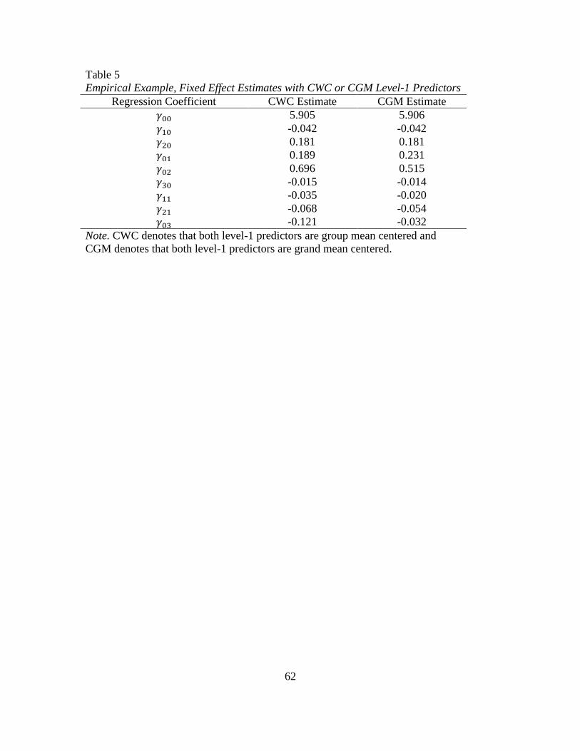
62

Table 5

Empirical Example, Fixed Effect Estimates with CWC or CGM Level-1 Predictors

Regression Coefficient CWC Estimate CGM Estimate

𝛾00 5.905 5.906

𝛾10 -0.042 -0.042

𝛾20 0.181 0.181

𝛾01 0.189 0.231

𝛾02 0.696 0.515

𝛾30 -0.015 -0.014

𝛾11 -0.035 -0.020

𝛾21 -0.068 -0.054

𝛾03 -0.121 -0.032

Note. CWC denotes that both level-1 predictors are group mean centered and

CGM denotes that both level-1 predictors are grand mean centered.

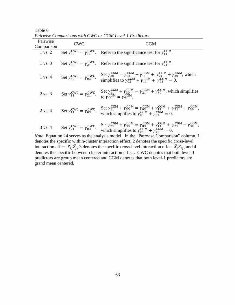
63

Table 6

Pairwise Comparisons with CWC or CGM Level-1 Predictors

Pairwise

Comparison CWC CGM

1 vs. 2 Set 𝛾30CWC = 𝛾11

CWC. Refer to the significance test for 𝛾11CGM.


CWC. Refer to the significance test for 𝛾21CGM.


CWC. Set 𝛾30

CGM = 𝛾03CGM + 𝛾11


CGM, which

simplifies to 𝛾03CGM + 𝛾11

CGM + 𝛾21CGM = 0.


CWC. Set 𝛾11


CGM + 𝛾30CGM, which simplifies

to 𝛾11CGM = 𝛾21

CGM.


CWC. Set 𝛾11



CGM + 𝛾30CGM,

which simplifies to 𝛾03CGM + 𝛾21

CGM = 0.


CWC. Set 𝛾21



CGM + 𝛾30CGM,

which simplifies to 𝛾03CGM + 𝛾11

CGM = 0.

Note. Equation 24 serves as the analysis model. In the “Pairwise Comparison” column, 1

denotes the specific within-cluster interaction effect, 2 denotes the specific cross-level

interaction effect 𝑋𝑖𝑗�̅�𝑗, 3 denotes the specific cross-level interaction effect �̅�𝑗𝑍𝑖𝑗, and 4

denotes the specific between-cluster interaction effect. CWC denotes that both level-1

predictors are group mean centered and CGM denotes that both level-1 predictors are

grand mean centered.

64

APPENDIX B

DERIVATIONS FROM DUNCAN, CUZZORT, AND DUNCAN (1961)

65

The equation of interest is Equation 3 from Duncan et al. (1961):

𝑏𝑇 = 𝜂𝑋2 𝑏𝐵 + (1 − 𝜂𝑋

2 )𝑏𝑊 (A1)

that describes how the level-1 regression coefficient 𝛾10 from Equation 2 (i.e., 𝑏𝑇) is a

weighted average of the within-cluster and between-cluster associations between the

level-1 predictor 𝑋𝑖𝑗 and the outcome variable. Although Duncan et al. (1961) do not

provide the following derivations for Equation A1, they provided the basis for these

derivations.

First I explain the notation used here, which deviates from the notation used in

Duncan et al. (1961). Let 𝑆𝑆𝑋𝑇 = ∑ ∑ (𝑋𝑖𝑗 − �̅�)2𝑖𝑗 denote the total sum of squares of 𝑋𝑖𝑗.

The total sum of squares of 𝑋𝑖𝑗 can be expressed as the sum of the within-cluster sum of

squares of 𝑋𝑖𝑗, 𝑆𝑆𝑋𝑊 = ∑ ∑ (𝑋𝑖𝑗 − �̅�𝑗)2𝑖𝑗 , and the between-cluster sum of squares of 𝑋𝑖𝑗,

𝑆𝑆𝑋𝐵 = ∑ ∑ (�̅�𝑗 − �̅�)2𝑖𝑗 , meaning

𝑆𝑆𝑋𝑇 = 𝑆𝑆𝑋𝑊 + 𝑆𝑆𝑋𝐵. (A2)

Let 𝑆𝑆𝑋𝑌𝑇 = ∑ ∑ (𝑋𝑖𝑗 − �̅�)(𝑌𝑖𝑗 − �̅�)𝑖𝑗 denote the total sum of products. The total sum of

products can be expressed as the sum of the within-cluster sum of products, 𝑆𝑆𝑋𝑌𝑊 =

∑ ∑ (𝑋𝑖𝑗 − �̅�𝑗)(𝑌𝑖𝑗 − �̅�𝑗)𝑖𝑗 , and the between-cluster sum of products, 𝑆𝑆𝑋𝑌𝐵 =

∑ 𝑛𝑗(�̅�𝑗 − �̅�)(�̅�𝑗 − �̅�)𝑗 , meaning

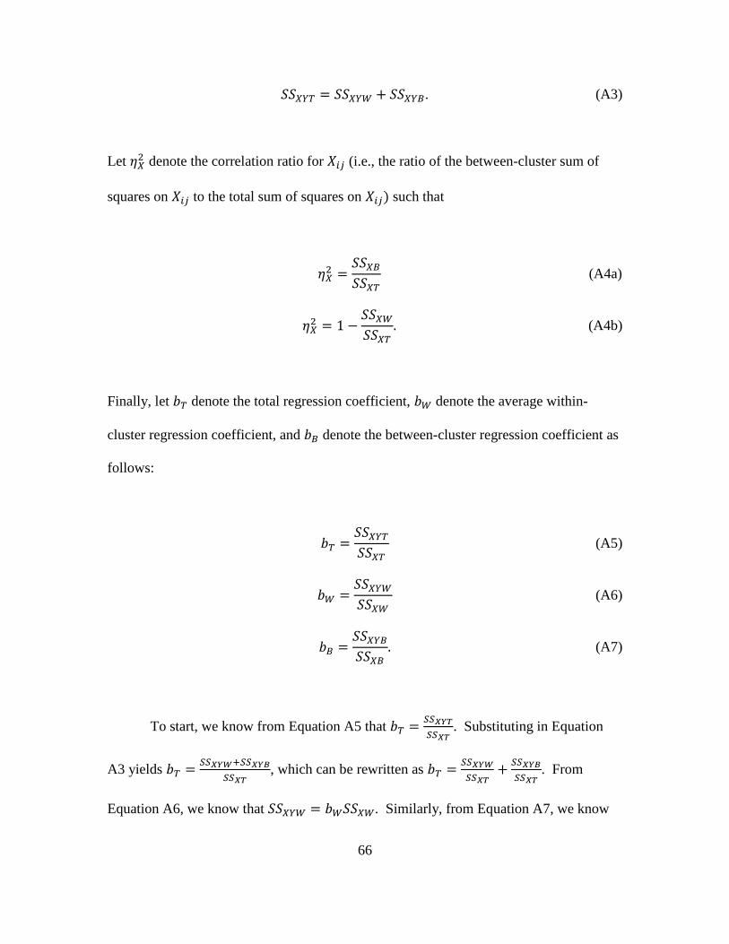
66

𝑆𝑆𝑋𝑌𝑇 = 𝑆𝑆𝑋𝑌𝑊 + 𝑆𝑆𝑋𝑌𝐵. (A3)

Let 𝜂𝑋2 denote the correlation ratio for 𝑋𝑖𝑗 (i.e., the ratio of the between-cluster sum of

squares on 𝑋𝑖𝑗 to the total sum of squares on 𝑋𝑖𝑗) such that

𝜂𝑋2 =

𝑆𝑆𝑋𝐵

𝑆𝑆𝑋𝑇 (A4a)

𝜂𝑋2 = 1 −

𝑆𝑆𝑋𝑊

𝑆𝑆𝑋𝑇. (A4b)

Finally, let 𝑏𝑇 denote the total regression coefficient, 𝑏𝑊 denote the average within-

cluster regression coefficient, and 𝑏𝐵 denote the between-cluster regression coefficient as

follows:

𝑏𝑇 =𝑆𝑆𝑋𝑌𝑇

𝑆𝑆𝑋𝑇 (A5)

𝑏𝑊 =𝑆𝑆𝑋𝑌𝑊

𝑆𝑆𝑋𝑊 (A6)

𝑏𝐵 =𝑆𝑆𝑋𝑌𝐵

𝑆𝑆𝑋𝐵. (A7)

To start, we know from Equation A5 that 𝑏𝑇 =𝑆𝑆𝑋𝑌𝑇

𝑆𝑆𝑋𝑇. Substituting in Equation

A3 yields 𝑏𝑇 =𝑆𝑆𝑋𝑌𝑊+𝑆𝑆𝑋𝑌𝐵

𝑆𝑆𝑋𝑇, which can be rewritten as 𝑏𝑇 =

𝑆𝑆𝑋𝑌𝑊

𝑆𝑆𝑋𝑇+

𝑆𝑆𝑋𝑌𝐵

𝑆𝑆𝑋𝑇. From

Equation A6, we know that 𝑆𝑆𝑋𝑌𝑊 = 𝑏𝑊𝑆𝑆𝑋𝑊. Similarly, from Equation A7, we know

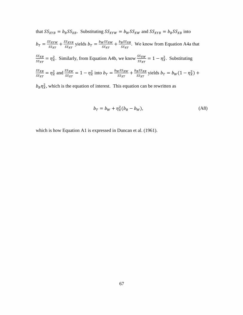
67

that 𝑆𝑆𝑋𝑌𝐵 = 𝑏𝐵𝑆𝑆𝑋𝐵. Substituting 𝑆𝑆𝑋𝑌𝑊 = 𝑏𝑊𝑆𝑆𝑋𝑊 and 𝑆𝑆𝑋𝑌𝐵 = 𝑏𝐵𝑆𝑆𝑋𝐵 into

𝑏𝑇 =𝑆𝑆𝑋𝑌𝑊

𝑆𝑆𝑋𝑇+

𝑆𝑆𝑋𝑌𝐵

𝑆𝑆𝑋𝑇 yields 𝑏𝑇 =

𝑏𝑊𝑆𝑆𝑋𝑊

𝑆𝑆𝑋𝑇+

𝑏𝐵𝑆𝑆𝑋𝐵

𝑆𝑆𝑋𝑇. We know from Equation A4a that

𝑆𝑆𝑋𝐵

𝑆𝑆𝑋𝑇= 𝜂𝑋

2 . Similarly, from Equation A4b, we know 𝑆𝑆𝑋𝑊

𝑆𝑆𝑋𝑇= 1 − 𝜂𝑋

2 . Substituting

𝑆𝑆𝑋𝐵

𝑆𝑆𝑋𝑇= 𝜂𝑋

2 and 𝑆𝑆𝑋𝑊

𝑆𝑆𝑋𝑇= 1 − 𝜂𝑋

2 into 𝑏𝑇 =𝑏𝑊𝑆𝑆𝑋𝑊

𝑆𝑆𝑋𝑇+

𝑏𝐵𝑆𝑆𝑋𝐵

𝑆𝑆𝑋𝑇 yields 𝑏𝑇 = 𝑏𝑊(1 − 𝜂𝑋

2 ) +

𝑏𝐵𝜂𝑋2 , which is the equation of interest. This equation can be rewritten as

𝑏𝑇 = 𝑏𝑊 + 𝜂𝑋2 (𝑏𝐵 − 𝑏𝑊), (A8)

which is how Equation A1 is expressed in Duncan et al. (1961).

68

APPENDIX C

DERIVATIONS FOR DEMONSTRATIVE SIMULATIONS

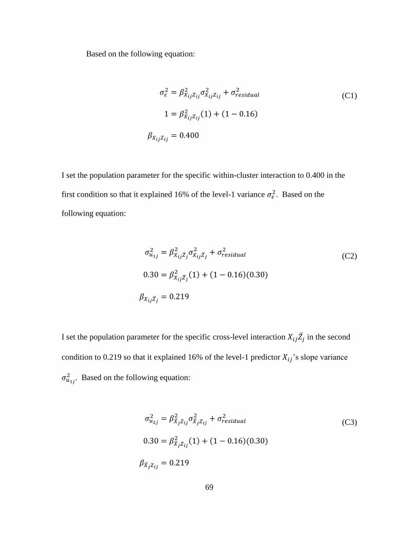
69

Based on the following equation:

𝜎𝜀2 = 𝛽𝑋𝑖𝑗𝑍𝑖𝑗

2 𝜎𝑋𝑖𝑗𝑍𝑖𝑗

2 + 𝜎𝑟𝑒𝑠𝑖𝑑𝑢𝑎𝑙2

1 = 𝛽𝑋𝑖𝑗𝑍𝑖𝑗

2 (1) + (1 − 0.16)

𝛽𝑋𝑖𝑗𝑍𝑖𝑗= 0.400

(C1)

I set the population parameter for the specific within-cluster interaction to 0.400 in the

first condition so that it explained 16% of the level-1 variance 𝜎𝜀2. Based on the

following equation:

𝜎𝑢1𝑗

2 = 𝛽𝑋𝑖𝑗𝑍𝑗

2 𝜎𝑋𝑖𝑗𝑍𝑗


0.30 = 𝛽𝑋𝑖𝑗𝑍𝑗

2 (1) + (1 − 0.16)(0.30)

𝛽𝑋𝑖𝑗𝑍𝑗= 0.219

(C2)

I set the population parameter for the specific cross-level interaction 𝑋𝑖𝑗�̅�𝑗 in the second

condition to 0.219 so that it explained 16% of the level-1 predictor 𝑋𝑖𝑗’s slope variance

𝜎𝑢1𝑗

2 . Based on the following equation:

𝜎𝑢2𝑗

2 = 𝛽�̅�𝑗𝑍𝑖𝑗

2 𝜎�̅�𝑗𝑍𝑖𝑗


0.30 = 𝛽�̅�𝑗𝑍𝑖𝑗

2 (1) + (1 − 0.16)(0.30)

𝛽�̅�𝑗𝑍𝑖𝑗= 0.219

(C3)

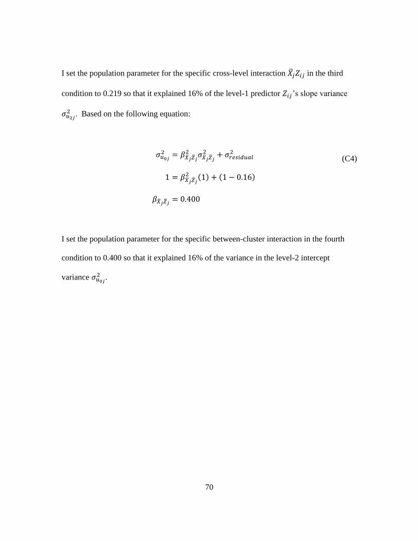
70

I set the population parameter for the specific cross-level interaction �̅�𝑗𝑍𝑖𝑗 in the third

condition to 0.219 so that it explained 16% of the level-1 predictor 𝑍𝑖𝑗’s slope variance

𝜎𝑢2𝑗

2 . Based on the following equation:

𝜎𝑢0𝑗

2 = 𝛽�̅�𝑗𝑍𝑗

2 𝜎�̅�𝑗𝑍𝑗


1 = 𝛽�̅�𝑗𝑍𝑗

2 (1) + (1 − 0.16)

𝛽�̅�𝑗𝑍𝑗= 0.400

(C4)

I set the population parameter for the specific between-cluster interaction in the fourth

condition to 0.400 so that it explained 16% of the variance in the level-2 intercept

variance 𝜎𝑢0𝑗

2 .

71

APPENDIX D

MPLUS 7.3 INPUT FILES FOR EMPIRICAL EXAMPLE

72

DATA:

! I applied CWC to the level-1 predictors and CGM to their cluster means in this data set.

file = CWC.dat;

VARIABLE:

! 1 indicates morning, 2 indicates afternoon, and 3 indicates evening.

names = paffm3 naffm2 work3 paffect3 naffect2 subject;

usevariables = paffm3 naffm2 work3 paffect3 naffect2

intwthn cross1 cross2 intbtwn;

cluster = subject;

within = naffect2 paffect3 intwthn cross1 cross2;

between = naffm2 paffm3 intbtwn;

missing = *;

DEFINE:

! Specific Within-Cluster Interaction Effect

intwthn = naffect2*paffect3;

! Specific Cross-Level Interaction Effects

cross1 = naffect2*paffm3;

cross2 = naffm2*paffect3;

! Specific Between-Cluster Interaction Effect

intbtwn = naffm2*paffm3;

ANALYSIS:

estimator = mlr;

type = twolevel random;

MODEL:

%within%

work3 on naffect2 paffect3 intwthn cross1 cross2;

work3;

%between%

work3 on naffm2 paffm3 intbtwn;

[work3];

work3;

MODEL TEST:

! Perform a Wald test to investigate whether the specific interaction effects are equal.

g30 = g11;

g30 = g21;

g30 = g03;

The MODEL TEST command below can be substituted into the Mplus input file above to

perform a pairwise comparison rather than an omnibus test.

73

MODEL TEST:

! Perform a Wald test to investigate whether the specific cross-level interaction effect

! and the specific between-cluster interaction are equal.

g21 = g03;

74

DATA:

! I applied CGM to the level-1 predictors and CGM to their cluster means in this data set.

file = CGM.dat;

VARIABLE:

names = paffm3 naffm2 paffect3 naffect2 work3 subject;

usevariables = work3 naffm2 paffm3 naffect2 paffect3

gamma30 gamma11 gamma21 gamma03;

cluster = subject;

within = naffect2 paffect3 gamma30 gamma11 gamma21;

between = naffm2 paffm3 gamma03;

missing = *;

DEFINE:

gamma30 = naffect2*paffect3;

gamma11 = naffect2*paffm3;

gamma21 = naffm2*paffect3;

gamma03 = naffm2*paffm3;

ANALYSIS:

estimator = mlr;

type = twolevel random;

MODEL:

%within%

work3 on naffect2 paffect3

gamma30 (g30)

gamma11 (g11)

gamma21 (g21);

work3;

%between%

work3 on naffm2 paffm3

gamma03 (g03);

[work3];

work3;

MODEL CONSTRAINT:

new (intwthn cross1 cross2 intbtwn);

! Specific Within-Cluster Interaction Effect

intwthn = g30;

! Specific Cross-Level Interaction Effects

cross1 = g11 + g30;

cross2 = g21 + g30;

! Specific Between-Cluster Interaction Effect

75

intbtwn = g03 + g11 + g21 + g30;

MODEL TEST:

! Perform a Wald test to investigate whether the specific interaction effects are equal.

g11 = 0;

g21 = 0;

g03 = 0;

←Alternative

Specifications→

intwthn = cross1;

intwthn = cross2;

intwthn =

intbtwn;

The MODEL TEST command below can be substituted into the Mplus input file above to

perform a pairwise comparison rather than an omnibus test.

MODEL TEST:

! Perform a Wald test to investigate whether the specific cross-level interaction effect

! and the specific between-cluster interaction are equal.

0 = g03 +

g11;

←Alternative

Specifications→ cross2 = intbtwn;

Interaction Effects in Multilevel Models by Gina L. Mazza A … · Interaction Effects in...

Documents

Transcript of Interaction Effects in Multilevel Models by Gina L. Mazza A … · Interaction Effects in...