intensity of competition and the choice between product and process innovation
26
1 Forthcoming in the International Journal of Industrial Organization INTENSITY OF COMPETITION AND THE CHOICE BETWEEN PRODUCT AND PROCESS INNOVATION * Giacomo Bonanno Department of Economics, University of California, Davis, CA 95616 - 8578, USA e-mail: [email protected] and Barry Haworth School of Economics and Public Affairs, University of Louisville, Louisville, KY 40292, USA e-mail: [email protected] Abstract Two questions are examined within a model of vertical differentiation. The first is whether cost-reducing innovations are more likely to be observed in regimes of more intense or less intense competition. Following Delbono and Denicolo (1990) and Bester and Petrakis (1993) we compare two identical industries that differ only in the regime of competition: Bertrand versus Cournot. Since Cournot competition leads to lower output and higher prices, it can be thought of as a regime of less intense competition. We find that the increase in profits associated with any given cost reduction is higher in the case of Cournot competition than in the case of Bertrand competition. Thus there are cost-reducing innovations that would be pursued under Cournot competition but not under Bertrand competition. The second question, which so far has not been analyzed in the literature, is what factors might be important in a firm’s decision whether to invest in product innovation (improvement in the quality of its product) or process innovation (cost reduction). We show that the regime of competition might be one such factor. For the high quality firm our result is that if there is a difference between the choice made by a Bertrand competitor and the choice made by a Cournot competitor, then the former will opt for product innovation, while the latter will prefer process innovation. For the low-quality firm, on the other hand, the result is reversed: whenever there is a difference, the Bertrand competitor will favor process innovation, while the Cournot competitor will favor product innovation. * We are grateful to two anonymous referees, Raymond De Bondt, Louis Makowski and Klaus Nehring for helpful comments and suggestions.
Transcript of intensity of competition and the choice between product and process innovation

1
Forthcoming in the International Journal of Industrial Organization
INTENSITY OF COMPETITION AND THE CHOICE BETWEEN PRODUCT AND PROCESS INNOVATION *
Giacomo Bonanno Department of Economics, University of California, Davis, CA 95616 - 8578, USA e-mail: [email protected]
and
Barry Haworth School of Economics and Public Affairs, University of Louisville, Louisville, KY 40292, USA e-mail: [email protected]
Abstract
Two questions are examined within a model of vertical differentiation. The first is whether cost-reducing innovations are more likely to be observed in regimes of more intense or less intense competition. Following Delbono and Denicolo (1990) and Bester and Petrakis (1993) we compare two identical industries that differ only in the regime of competition: Bertrand versus Cournot. Since Cournot competition leads to lower output and higher prices, it can be thought of as a regime of less intense competition. We find that the increase in profits associated with any given cost reduction is higher in the case of Cournot competition than in the case of Bertrand competition. Thus there are cost-reducing innovations that would be pursued under Cournot competition but not under Bertrand competition.
The second question, which so far has not been analyzed in the literature, is what factors might be important in a firm’s decision whether to invest in product innovation (improvement in the quality of its product) or process innovation (cost reduction). We show that the regime of competition might be one such factor. For the high quality firm our result is that if there is a difference between the choice made by a Bertrand competitor and the choice made by a Cournot competitor, then the former will opt for product innovation, while the latter will prefer process innovation. For the low-quality firm, on the other hand, the result is reversed: whenever there is a difference, the Bertrand competitor will favor process innovation, while the Cournot competitor will favor product innovation.
* We are grateful to two anonymous referees, Raymond De Bondt, Louis Makowski and Klaus Nehring for helpful comments and suggestions.
2
1. Introduction
There is a vast literature on the economic aspects of innovation. A wide spectrum
of issues has been analyzed, from the timing of innovative ventures, to expenditure
patterns in R&D races, to spillover effects and their impact (for an excellent survey of the
latter see De Bondt, 1995). The issue we address in this paper is the relationship between
intensity of competition and the profitability of innovative activity. A traditional line of
reasoning, associated with Schumpeter (1943), is that market concentration is a stimulus
to innovation. An early challenge to this view came from Arrow (1962), who sought to
establish the reverse proposition that more competitive environments would give a
greater incentive to innovate. Arrow considered the case of a firm undertaking a cost-
reducing investment that cannot be imitated by competitors. He compared a monopoly
with a perfectly competitive industry, under the same demand and cost conditions, and
showed that the gain from a cost-reducing innovation is higher for a firm in the latter than
for the monopolist. A more interesting comparison would be between two oligopolistic
industries. It is not clear, however, how “intensity of competition” can be measured in
such a setting. Delbono and Denicolo (1990) and Bester and Petrakis (1993) suggested
comparing two industries (with the same number of firms and the same linear demand
and cost functions) under different regimes of competition: Cournot (where firms’
decision variables are output levels) and Bertrand (where firms’ decision variables are
prices). Since Cournot competition normally leads to lower output and higher prices than
Bertrand competition, one can think of the former as a situation where competition is less
intense. Delbono and Denicolo (1990) showed that, under the assumption of a
homogeneous product, the incentive to introduce a cost-reducing innovation is greater for
a Bertrand competitor than for a Cournot competitor: an “Arrow-like” result. Bester and
Petrakis (1993), on the other hand, considered the case of differentiated products and

3
obtained a mixed result: if the degree of differentiation is “large”, the incentive to
introduce a cost-reducing innovation is higher for the Cournot competitor, while if the
degree of differentiation is “small”, then the incentive is higher for a Bertrand competitor.
Bester and Petrakis’s model is one of horizontal differentiation (when prices are
equal both products enjoy positive demand). In the first part of the paper we re-examine
the issue within a model of vertical differentiation (if prices are equal, only one product
− the higher quality one − enjoys positive demand) and show that the increase in profits
associated with any given cost reduction is higher in the case of Cournot competition than
in the case of Bertrand competition, and this is true no matter how small the degree of
differentiation (thus even if the products are virtually homogeneous). It follows that there
are cost-reducing innovations that would be pursued under Cournot competition but not
under Bertrand competition (a “Schumpeter-like” result).
In the second part of the paper we address a related issue, which − somewhat
surprisingly − has received very little attention in the literature. It is customary to
distinguish between two types of innovation: product and process innovation. The former
consists in the creation of new goods and services, while the latter leads to a reduction in
the cost of producing existing products. The literature has dealt primarily with overall
innovative activity (that is, the sum of product and process innovation) or one specific
type of innovative activity (either process or product innovation).1 There have been no
attempts to explain what factors might be important in a firm’s decision whether to direct
R&D expenditure towards product innovation or towards process innovation 2. In this
1 See surveys by Kamien and Schwartz (1975), Baldwin and Scott (1987), Cohen and Levin (1989), Scherer and Ross (1990) and Tirole (1988).
2 An exception is Rosenkrantz (1995) which is discussed in Section 5. We are grateful to Raymond De Bondt for bringing this paper to our attention.

4
paper we take a first step in the direction of filling this gap, by providing an explanation
based on the type of competitive regime in which the firms find themselves (Cournot vs.
Bertrand). We shall think of product innovation as an improvement in the quality of a
firm’s product (e.g. the introduction of a faster computer chip). Process innovation will be
interpreted as a reduction in the firm’s costs. We show that, if the choice is between a
given cost reduction or a given quality improvement and the innovator is the high quality
firm, one of three things can happen: (1) both the Cournot competitor and the Bertrand
competitor choose the cost reduction, or (2) both choose the quality improvement, or (3)
they make different choices, in which case the Cournot competitor chooses the cost
reduction, while the Bertrand competitor chooses the quality improvement. That is, if
Bertrand competition and Cournot competition lead to different choices, then the
Bertrand competitor will favor product innovation, while the Cournot competitor will opt
for process innovation. On the other hand, if the innovator is the low quality firm, then
the opposite is true: whenever the two regimes of competition yield different choices, the
Bertrand competitor will choose process innovation, while the Cournot competitor will
choose product innovation.
The paper is organized as follows. Section 2 develops the model, Section 3 deals
with cost-reducing innovations, while Section 4 is concerned with the choice between
process and product innovation. Section 5 contains some final remarks and a conclusion.
The proofs of all the results are omitted and can be obtained from the authors.
2. A model of vertical differentiation
We use a model of vertical differentiation introduced by Mussa and Rosen (1978).
There are N consumers with the same income, denoted by E, but different values of the

5
taste parameter θ. Each consumer buys at most one unit. If a consumer does not buy the
product, her utility is equal to her income E. If a consumer with parameter θ buys one unit
of a good of quality k, at price p, her utility is equal to E − p + θ k. The parameter θ is
uniformly distributed in the interval (0,1]. It follows that, for every x∈(0,1], the number
of consumers with parameter θ less than or equal to x is xN. We consider the case where
there are two firms. Firm H sells a product of quality kH while firm L sells a product of
quality kL, with k
H > k
L > 0 (thus ‘H’ stands for ‘high quality’ and ‘L’ for ‘low quality’).
Let pi be the price charged by firm i (i=H,L). The demand functions are obtained as
follows. Let θ0 be the value of θ for which the corresponding consumer is indifferent
between consuming nothing and consuming the low-quality product. Then θ0 is the
solution to the equation
E = E − pL + θ k
L.
Thus θ0 =
pL
kL . Let θ
1 be the value of θ for which the corresponding consumer is
indifferent between buying the low-quality product and the high-quality one. Then θ1 is
the solution to the equation
E − pL + θ k
L = E − p
H + θ k
H .
Thus θ1 =
pH − p
L
kH − k
L
. Hence the (direct) demand functions are given by
D p p Np p
k kN
D p p Np p
k k
p
kN
H H LH L
H L
L H LH L
H L
L
L
( , ) ( )
( , ) ( )
= − = −−−
= − =−−
−
1 11
1 0
θ
θ θ
Like Bester and Petrakis (1993) and Rosenkrantz (1995) we assume that the two firms
operate under constant returns to scale. Thus firm i (i=H,L) has a cost function of the

6
form Ci(q
i) = c
iq
i with c
i>0. We also assume that higher quality is associated with higher
costs: cH > c
L. Finally, we assume that c
H and c
L are such that both demands are positive
when the two products are sold at unit cost (i.e. when pH = c
H and p
L = c
L).3 It is easy to
see that this is the case if and only if the following two conditions are satisfied 4
kH − k
L > cH
− cL (1a)
and
kL
cH > k
H c
L (1b).
The inverse demand functions are given by (where qH denotes the output of firm H and q
L
the output of firm L)
f q qNk k q k q
N
f q qk N q q
N
H H LH H H L L
L H LL H L
( , )
( , )( )
=− −
=− −
We consider two cases: the Bertrand case (decision variables are prices) and the Cournot
case (decision variables are output levels). We shall use superscript ‘B’ for the Bertrand
case and superscript ‘C’ for the Cournot case.
In the Bertrand case the profit functions are given by
3 This assumption guarantees that at all the equilibria we consider, prices and output levels are positive: cf. Remark 1 below.
4 Note that (1a) and (1b) imply that cH < k
H and c
L < k
L.

7
Π
Π
HB
H L H HH L
H L
LB
H L L LH L
H L
L
L
p p N p cp p
k k
p p N p cp p
k k
p
k
( , ) ( )
( , ) ( )
= − −−−
= −−−
−
1
(2)
Prices and output levels at the Bertrand-Nash equilibrium are given by
pk k k c c
k k
pk k k c k k c
k k
HB H H L H L
H L
LB H L L H L H L
H L
=− + +
−
=− + +
−
( )
( )
2 2 2
4
2
4
2
q Nk k k k c k c k c
k k k k
q Nk k k k k c k c k c
k k k k k
HB H H L H H H L L H
H L H L
LB H H L L L H H L L L
H L H L L
=− − + +
− −
=− + − +
− −
( )
( )( )
( )
( )( )
2 2 2
4
2
4
2
2
(3)
giving the following expressions for the equilibrium profits of firms H and L:
( )
( )
π
π
HB
H L H LH H L H H H L L H
H L H L
H LHB
LB
H L H L HH L L H L L L L H
H L H L L
L H L
HLB
k k c c Nk k k k c k c k c
k k k k
k k
Nq
k k c c Nkk k k k c k c k c
k k k k k
k k k
k Nq
( , , , )[ ]
( ) ( )
( , , , )[ ]
( ) ( )
( )
=− − + +
− −=
−
=− − + +
− −=
−
2 2 2
4
2
4
2 2
2
2
2 2
2
2
(4)
We now move to the Cournot case, where the profit functions are given by
Π
Π
HC
H L HH H H L L
H
LC
H L LL H L
L
q q qNk q k q k
Nc
q q qk N q q
Nc
( , )
( , )( )
=− −
−
=− −
−
Prices and output levels at the Cournot-Nash equilibrium are given by

8
pk k k k c k c c k
k k
pk k k c k c k c
k k
HC H H L H H H L H L
H L
LC H L H L L H L L
H L
=− + + −
−
=+ + −
−
2 2
4
2
4
2
q Nk k c c
k k
q Nk k k c k c
k k k
HC H L H L
H L
LC H L L H H L
H L L
=− − +
−
=+ −
−
2 2
4
2
4( )
(5)
yielding the following expressions for the equilibrium profits of firms H and L:
( )
( )
π
π
HC
H L H LH H L H L
H L
HHC
LC
H L H LH L H L L H
H L L
LLC
k k c c Nk k k c c
k k
k
Nq
k k c c Nk k k c k c
k k k
k
Nq
( , , , )( )
( )
( , , , )( )
( )
=− − +
−=
=− +
−=
2 2
4
2
4
2
2
2
2
2
2
(6)
REMARK 1. The following facts can be checked easily. If the parameter
restrictions (1a) and (1b) are satisfied, then, for each firm i (i=H,L), Cournot output is
smaller than Bertrand output (qCi < q
Bi ), Cournot price is higher than Bertrand price
(pCi > p
Bi ), and Cournot profit is higher than Bertrand profit (πC
i > πBi ). Furthermore, all
these quantities are positive and equilibrium prices are greater than unit cost
(pCi > p
Bi > c
i).
3. Intensity of competition and the profitability of cost-reducing innovations
In this section we compare the incentives for a given cost reduction between a
Bertrand competitor and a Cournot competitor and show that the latter is larger. Let ∆H >
0 be a non-drastic cost reduction for firm H and ∆L > 0 a non-drastic cost reduction for
firm L, where “non-drastic” means that after the cost reduction the innovator cannot drive
the other firm out of the market by charging a price close to unit cost. That is, we assume

9
that ∆H and ∆
L are sufficiently small for inequalities corresponding to (1a) and (1b) to be
satisfied:
kH − k
L > (c
H − ∆
H) − c
L (7a)
kL ( c
H − ∆
H) > k
H c
L (7b)
kH − k
L > c
H − ( c
L − ∆
L) (7c)
kLc
H
> k
H (c
L− ∆
L) (7d)
For each firm i (i = H,L), let ∆π Ci be the increase in profits expected from the
given cost reduction in the case of Cournot competition and ∆π Bi the increase in profits
expected from the given cost reduction in the case of Bertrand competition:
∆π CH = πC
H (kH, k
L, c
H− ∆H, c
L) − πC
H (kH, k
L, c
H, c
L) (8a)
∆π BH = πB
H (kH, k
L, c
H− ∆H, c
L) − πB
H (kH, k
L, c
H, c
L) (8b)
∆π CL = πC
L (kH, k
L, c
H, c
L− ∆L) − πC
L (kH, k
L, c
H, c
L) (8c)
∆π BL = πB
L (kH, k
L, c
H, c
L− ∆L) − πB
L (kH, k
L, c
H, c
L) (8d)
where πCH and πC
L are given by (6) and πBH and πB
L are given by (4).
The following remark confirms Bester and Petrakis’s result (1993, p. 525,
Proposition 1) that the marginal return on investment in a cost reduction is increasing.
REMARK 2. ∆π CH and ∆π B
H are decreasing in cH and ∆π C
L and ∆π BL are
decreasing in cL.
Proposition 1 below gives a “Schumpeter-like” result: less intense competition is
associated with a greater propensity to introduce cost-reducing innovations. Define a cost-

10
reducing investment opportunity for firm i (i = H, L) as a pair (∆i, α) where α is the cost
of implementing the innovation and ∆i is the reduction in unit cost expected from the
innovation. It is clear that firm i will carry out the investment if and only if the expected
increase in profits is greater than the implementation cost, that is, if and only if ∆πi > α.
PROPOSITION 1. For each i (i = H, L) there are cost-reducing investment
opportunities that are carried out by firm i if it operates in a regime of Cournot
competition but not if it operates in a regime of Bertrand competition. On the other hand,
every cost-reducing investment carried out under Bertrand competition is also carried out
under Cournot competition.
Proposition 1 follows directly from the following fact: for all kH, k
L, c
H, c
L, ∆H
and ∆L that satisfy (7), and for every i = H,L, ∆π C
i > ∆π Bi . The intuition behind
Proposition 1 is as follows. A cost reduction by firm i has a direct (positive) effect on the
profits of firm i as well as a strategic or indirect effect through the change it induces in
the choice variable of the competitor. In a Bertrand regime the strategic effect is negative:
the competitor will respond to a reduction in ci by reducing its own price, thereby
increasing the intensity of competition5. In a Cournot regime on the other hand, a cost
5 The strategic effect is given by ∂∂
∂∂
Π iB
j
jB
ip
p
c where i ≠ j, Π i
B is given by (2) and piB is given
by (3). It is straightforward to verify that ∂∂
Π iB
jp> 0 and
∂∂
p
cjB
i
> 0 so that ∂∂
∂∂
Π iB
j
jB
ip
p
c> 0 . In the
terminology of Bulow et al (1985), in the Bertrand case (with linear demand) prices are strategic complements: a reduction in c
i leads to a reduction in p
i which in turn leads to a reduction in p
j, that is, an
“aggressive” response by the competitor.

11
reduction has positive strategic effects, that is, it leads to a softening of competition6.
Note that Proposition 1 holds no matter how small the degree of product differentiation,
that is, no matter how close kL is to k
H. Thus in a model of vertical differentiation the
mixed result obtained by Bester and Petrakis (1993) does not hold.
4. On the choice between process and product
innovation
We now turn to the choice between process and product innovation. Assume that
one of the two firms, say firm H, has invested in R&D (e.g. it has hired a team of
engineers) and the corresponding cost is sunk. Suppose that the firm has two options:
(1) it can instruct its researchers to pursue product innovation, expected to lead to an
increase in the quality of the firm’s product from k^ H to k
^ H + ∆k
(with ∆k > 0); or
(2) it can instruct them to pursue process innovation, expected to lead to a reduction
in the firm’s unit cost from c H to c
H− ∆ c (with 0 < ∆c ≤ c
H).
Assume that there are no other costs involved in the implementation of the innovation.
The choice facing the firm is illustrated in Figure 1. For example, the firm’s product
could be a computer chip with quality represented by the operating speed (measured in
MHz) and the choice could be between increasing the speed from 166 MHz to 200 MHz
or reducing the unit cost of its present product (the 166 MHz chip) from $800 to $720.
Define a product / process investment opportunity as a triple (∆c, ∆k, α) where α is the
6 The strategic effect is given by ∂∂
∂∂
Π iC
j
jC
iq
q
c which is negative, as one can easily verify (cf., in
particular, (5)). In the terminology of Bulow et al (1985), in the Cournot case (with linear demand) output levels are strategic substitutes: a reduction in c
i leads to an increase in q
i which in turn leads to a reduction
in qj, that is, a “submissive” response by the competitor.

12
cost of implementing the innovation (e.g. the cost of hiring a team of researchers), which
is the same for both types of innovation, ∆c is the expected reduction in unit cost if
process innovation is pursued (e.g. if the researchers are instructed to seek a cheaper
production process for the existing product) and ∆k is the expected quality increase if
product innovation is pursued (e.g. if the researchers are instructed to improve the quality
of the product). A process / product investment opportunity (∆c, ∆k, α) is profitable if the
expected increase in profits from at least one of the two types of innovation (cost
reduction or quality improvement) is greater than α, the (common) cost of implementing
the innovation. We shall first consider the case where the innovator is the high quality
firm. The following proposition states that a Bertrand competitor is more prone to choose
product innovation, while a Cournot competitor is more prone to choose process
innovation.
PROPOSITION 2. The following is true for the high-quality firm. Given a
profitable product / process investment opportunity (∆c, ∆k, α), either both the Bertrand
and the Cournot competitor choose the same type of innovation or, if they make different
choices then the Bertrand competitor chooses product innovation, while the Cournot
competitor chooses process innovation.
As illustrated in Figure 1, Proposition 2 follows from the following fact which
applies to the high-quality firm. Fix arbitrary k− H, k
− L , c
− H and c
− L that satisfy restrictions
(1a) and (1b); then in the (kH,c
H)-plane both the Bertrand isoprofit curve [obtained from
(4)] and the Cournot isoprofit curve [obtained from (6)] that go through the point ( k− H,
c −
H) are increasing; furthermore, the Bertrand isoprofit curve is steeper (at that point)
than the Cournot isoprofit curve. It follows that the two isoprofit curves cannot cross

13
more than once. Figure 1 shows the three possible cases7. Case 1 (Figure 1a): both the
Bertrand competitor and the Cournot competitor choose product innovation. Case 2
(Figure 1b): both the Bertrand competitor and the Cournot competitor choose process
innovation. Case 3 (Figure 1c): the Bertrand competitor and the Cournot competitor
make different choices. In this case the Bertrand competitor opts for product innovation,
while the Cournot competitor chooses process innovation.
k
c
H
H
kH
^
cH
^
Bertrandiso-profit curve
Cournotiso-profit curve
product innovation
process innovation
status quo
direction ofincreasingprofits
Figure 1a
7 It is useful to consider not the isoprofit curve that goes through the status quo (or pre-innovation) point, but rather the isoprofit curve that goes through the point that represents process innovation.

14
k
c
H
H
kH
^
cH
^
Bertrandiso-profit curve
Cournotiso-profit curve
product innovation
process innovation
status quo
direction ofincreasingprofits
Figure 1b
k
c
H
H
kH
^
cH
^
Bertrandiso-profit curve
Cournotiso-profit curve
product innovation
process innovation
status quo
direction of increasing profits
Figure 1c

15
The proof of Proposition 2 involves a number of rather complex algebraic manipulations which
are hard to interpret. To obtain some intuition as to why a Bertrand competitor has a propensity to favor
product over process innovation, recall that in a Bertrand regime a cost reduction has a negative strategic
effect, in that it leads to an intensification of competition (see Section 2), with the consequence that at
the equilibrium following process innovation both firms charge lower prices than at the pre-innovation
equilibrium. Product innovation, on the other hand, will always lead to an increase in the price of firm H
(the innovator), even though the equilibrium price of firm L (the competitor) may increase or decrease,
as shown in Figure 2. Of course, this intuitive explanation is only partially correct for three reasons:
(1) as shown in Figure 1b, even a Bertrand competitor will choose process innovation over product
innovation if the former “dominates” the latter (thus one can only speak of a tendency of Bertrand
competitors to favor product innovation), (2) the analogous intuition for the Cournot competitor cannot
be established, since both product and process innovation have a positive strategic effect, as shown in
Figure 3 and (3) it is easier to understand a comparison between regimes of competition holding the type
of innovation fixed (as we did in Section 2) than a comparison of different types of innovation holding
the regime of competition fixed (as we are doing here), because there is no obvious way of making a
change in quality (e.g. an increase of 34 MHz) directly comparable with a cost reduction (e.g. $80).
price of firm H
price of firm L
reaction curveof firm H BEFOREproduct innovation
reaction curveof firm H AFTER product innovation
possiblereaction curvesof firm L AFTER firm H's productinnovation
possible post-innovation equilibria
pre-innovationequilibrium
reaction curveof firm L BEFORE firm H's productinnovation
ΑΒ
Figure 2
The effect of product innovation in the Bertrand case when the innovator is firm H

16
output of firm H
output of firm L
reaction curveof firm H BEFOREprocess innovation
reaction curveof firm H AFTER process innovation
reaction curveof firm L
pre-innovation equilibrium
post-innovation equilibrium
Figure 3a
The effect of process innovation in the Cournot case when the innovator is firm H
output of firm H
output of firm L
reaction curveof firm H BEFOREproduct innovation
reaction curveof firm H AFTER product innovation
reaction curveof firm L
pre-innovation equilibrium
post-innovation equilibrium
Figure 3b
The effect of product innovation in the Cournot case when the innovator is firm H

17
We now turn to the case where the innovator is the low quality firm.
PROPOSITION 3. The following is true for the low-quality firm. Given a
profitable product / process investment opportunity (∆c, ∆k, α), either both the Bertrand
and the Cournot competitor choose the same type of innovation or, if they make different
choices then the Bertrand competitor chooses process innovation, while the Cournot
competitor chooses product innovation.
Proposition 3 follows from the following fact which applies to the low-quality
firm. Fix arbitrary k− H, k
− L , c
− H and c
− L that satisfy restrictions (1a) and (1b). Then in the
(kL,c
L)-plane the Cournot isoprofit curve [obtained from (6)] that goes through the point
( k −
L, c −
L) is increasing and steeper (at that point) than the Bertrand isoprofit curve
[obtained from (4)] that goes through the same point. Note that, while the Cournot
isoprofit curve is always increasing, the Bertrand isoprofit curve might not be (it will be
increasing if the degree of differentiation is not too small). Indeed, it has been shown in
the literature (Gabszewicz and Thisse, 1979, 1980; Shaked and Sutton, 1982 ) that when
there is Bertrand competition a low-quality firm might refrain from increasing the quality
of its product even if it could do so at zero cost. This will happen when the degree of
differentiation is very small. On the other hand, when competition is Cournot style, the
low-quality firm does have an incentive to increase the quality of its product (Bonanno,
1986). The comparison between process and product innovation is therefore interesting
mainly in the case where the low quality firm would profit from a costless quality
improvement (that is, when the Bertrand iso-profit curve is increasing). In this case we
have a reversal of the result of Proposition 2: when the innovator is the low-quality firm
and the Bertrand competitor makes a different choice from the Cournot competitor, then

18
the latter will opt for product innovation, while the former will choose process
innovation.
As for the case of Proposition 2, the proof of Proposition 3 involves a number of
complex algebraic manipulations which are hard to interpret. Some intuition for the result
can be obtained by examining the strategic effects. Consider, for example, the case of
Bertrand competition. Process innovation by the low-quality firm has negative strategic
effects, since it induces the innovator to reduce its price (firm L’s reaction curve shifts
down) and the competitor (firm H) will respond by also lowering its price. Product
innovation by firm L, on the other hand, would potentially have positive strategic effects,
since it shifts the innovator’s reaction curve up. However, unlike the case of Proposition 2
− where a quality improvement by the high quality firm increased the degree of
differentiation − here a quality improvement by firm L reduces the degree of
differentiation and induces an aggressive response by the competitor: the reaction curve
of firm H shifts to the left. To put it differently, a cost reduction for firm L has only an
indirect effect on firm H’s profits, through a reduction in the price of the innovator. A
quality improvement by firm L, on the other hand, has a direct effect on the competitor’s
profits (it reduces firm H’s revenue) and therefore induces a more aggressive response by
firm H.
5. Conclusion
Within a model of vertical differentiation (due to Mussa and Rosen, 1978) we
examined two issues. The first, which has received considerable attention in the literature,
is whether more intense competition is associated with a stronger or weaker incentive to
introduce a cost-reducing innovation. Following Delbono and Denicolo (1990) and Bester

19
and Petrakis (1993) we compared two identical industries (same demand and cost
functions, same number of firms) that differed only in the regime of competition:
Bertrand style versus Cournot style. Since Cournot competition leads to lower output and
higher prices than Bertrand competition, it can be thought of as a regime of less intense
competition. Our finding was that the incentive to introduce a cost-reducing innovation is
stronger for a Cournot competitor.
We then turned to an issue that so far has received little attention in the literature,
namely what factors might be important in a firm’s decision whether to invest in product
innovation (improvement in the quality of its product) or process innovation (cost
reduction). We found that the regime of competition might be one such factor. For the
high quality firm our result is that if there is a difference between the choice made by a
Bertrand competitor and the choice made by a Cournot competitor, then the former will
opt for product innovation, while the latter will prefer process innovation. For the low-
quality firm, on the other hand, the result is reversed: whenever there is a difference, the
Bertrand competitor will favor process innovation, while the Cournot competitor will
favor product innovation.
As far as we know, the only other paper in the literature that deals with the choice
between process and product innovation is Rosenkrantz (1995). She considers a model of
horizontal differentiation, similar to the model used by Bester and Petrakis (1993). A
two-stage Cournot duopoly model is considered where in stage 1 the firms
simultaneously choose their unit cost ci and their product characteristic d
i (the choice of c
i
is called process innovation and the choice of di is called product innovation); in the
second stage the firms choose outputs. Note, therefore, the following substantial
differences: (1) for us product innovation means an improvement in the quality of the
product (ours is a model of vertical differentiation), while for Rosenkrantz product
innovation means a change in the horizontal characteristic of the product; (2) while we
20
compare the investment choice of one firm in different regimes of competition (Bertrand
versus Cournot), Rosenkrantz analyzes the simultaneous choices of both firms within the
same regime of competition (Cournot); (3) while we assume that the firm is faced with
the choice between product and process innovation, Rosenkrantz allows each firm to mix
both types of innovation and is interested in studying how the optimal mix varies with the
parameters of the model (in particular the consumers’ reservation price).
A natural question to ask is: how robust are these results? The answer to this
question is two-fold. First of all, one cannot hope to obtain any results whatsoever in a
very general model where properties of demand and costs are specified only qualitatively.
The reason is that one needs to compare equilibria and in order to do so one needs to be
able to compute them. Indeed the model used in this paper is as “general” as the models
used in the literature on this topic (e.g. Delbono and Denicolo, 1990, Bester and Petrakis,
1993 and Rosenkrantz, 1995). The type of issues considered can only be analyzed in
models that have a lot of structure and the richer the structure the less general the model.
Secondly, although the model is rather specific, the results can be understood (fully, as in
the case of Proposition 1 or only partially, as in the case of Propositions 2 and 3) in terms
of qualitative properties, such as the strategic effects of different types of innovation.

21
References Arrow, K. (1962), Economic welfare and the allocation of resources for inventions. in: R.
Nelson (Ed.), The rate and direction or inventive activity, Princeton University Press, Princeton, NJ.
Baldwin, W.L. and J.T. Scott (1987), Market structure and technological change, Harwood Academic Publishers, Chur (Switzerland).
Bester, H. and E. Petrakis (1993), The incentives for cost reduction in a differentiated industry, International Journal of Industrial Organization, 11, 519-534.
Bonanno, G. (1986), Vertical differentiation with Cournot competition, Economic Notes, 15, 68-91.
Bulow, J., J. Geanakoplos and P. Klemperer (1985), Multimarket oligopoly: Strategic substitutes and complements, Journal of Political Economy, 93, 488-511.
Cohen, W. and R.C. Levin (1989), Empirical studies in innovation and market structure, in: R. Schmalensee and R.D. Willig (Eds.), Handbook of industrial organization, Vol. 2, Elsevier Science Publishers, Amsterdam.
De Bondt, R. (1995), Spillovers and innovative activities, mimeo, Katholieke Universiteit Leuven.
Delbono, F. and V. Denicolo (1990). R &D investment in a symmetric and homogeneous oligopoly, International Journal of Industrial Organization, 8, 297-313.
Gabszewicz, J and J-F. Thisse (1979), Price competition, quality and income disparities, Journal of Economic Theory, 20, 340-359.
Gabszewicz, J and J-F. Thisse (1980), Entry (and exit) in a differentiated industry, Journal of Economic Theory , 22, 327-338.
Kamien, M.I. and N.L. Schwartz (1975), Market structure and innovation: a survey, Journal of Economic Literature, 13, 1-37.
Mussa, M. and S. Rosen (1978), Monopoly and product quality, Journal of Economic Theory, 18, 301-317.
Rosenkrantz, S. (1995), Simultaneous choice of process and product innovation, mimeo, Wissenschaftszentrum, Berlin.
Shaked, A. and J. Sutton (1982), Relaxing price competition through product differentiation, Review of Economic Studies, 49, 3-13.
Scherer, F.M. and D. Ross (1990), Industrial market structure and economic performance, Houghton Mifflin Company, Boston.
Schumpeter, J. (1943), Capitalism. socialism and democracy, Allan and Unwin, London.
Tirole, J. (1988), The theory of industrial organization, M.I.T. Press, Cambridge.

22
Proofs of results in Bonanno-Haworth “Intensity of competition and the choice between product and process innovation”
(for Referees’ use: not meant for publication)
Proof of Proposition 1. We need to show that ∆π CH − ∆π B
H > 0 (where ∆π CH and
∆π BH are given by (8a) and (8b), respectively) and ∆π C
L − ∆π BL > 0 (where ∆π C
L and ∆π BL
are given by (8c) and (8d), respectively). Straightforward manipulations lead to:
∆π CH − ∆π B
H = − )]()[()()4( 2 HLHLLHHLLH
LHLH
HL kckckckckkkkk
Nk ∆+−+−−−
∆ (A1a)
∆π CL − ∆π B
L = Nk k
k k k kk k c cH L L
H L H LH L H L L
∆∆
( ) ( )[ ( ) ( ) ]
42 2
2− −− − − − (A1b)
The fractions in both expressions are positive (since kH > k
L > 0). The term in square brackets in
(A1a) is negative, since its first term is negative by (1b) and its second term is negative by (7b). The term in square brackets in (A1b) is positive since it is greater than 2[(k
H− k
L)− ( c
H− c
L+ ∆
L)],
which is positive by ( 7c).
Proof of Proposition 2. Fix arbitrary kH, k
L, c
H, c
L subject to the restrictions (1). Using the
implicit function theorem the slope of the Bertrand isoprofit curve at this point is given by:
−
∂ π∂∂ π∂
HB
H
HB
H
k
c
(A2)
where πBH is given by (4). Similarly, the slope of the Cournot isoprofit curve is equal to (where πC
H is given by (6))
−
∂ π∂∂ π∂
HC
H
HC
H
k
c
(A3)
We want to show that (A2) and (A3) are positive and that (A2) is greater than (A3). From (4) we get that
∂ π∂
HB
H
H L
H L H Lc
N k k
k k k k= −
−− −
Φ2 2
4 2
( )
( ) ( ) (Α4)
where
23
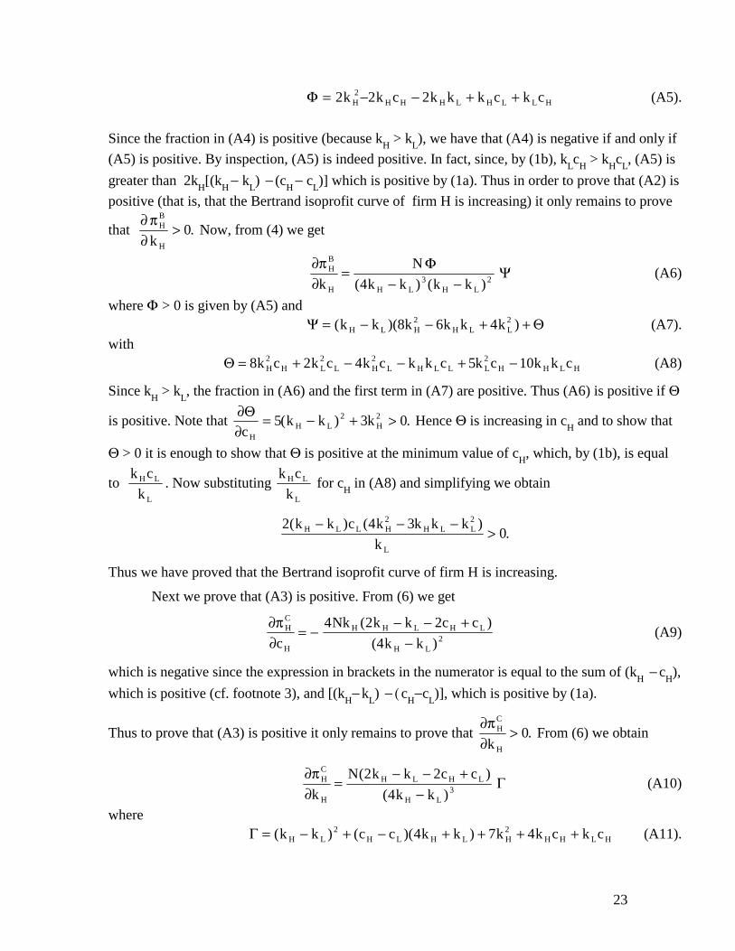
Φ = − − + +2 2 22k k c k k k c k cH H H H L H L L H (A5).
Since the fraction in (A4) is positive (because kH > k
L), we have that (A4) is negative if and only if
(A5) is positive. By inspection, (A5) is indeed positive. In fact, since, by (1b), kLc
H > k
Hc
L, (A5) is
greater than 2kH[(k
H− k
L) − (c
H− c
L)] which is positive by (1a). Thus in order to prove that (A2) is
positive (that is, that the Bertrand isoprofit curve of firm H is increasing) it only remains to prove
that ∂ π∂
HB
Hk> 0. Now, from (4) we get
∂π∂
HB
H H L H Lk
N
k k k k=
− −Φ
Ψ( ) ( )4 3 2 (A6)
where Φ > 0 is given by (A5) and Ψ Θ= − − + +( )(8 )k k k k k kH L H H L L
2 26 4 (A7). with
Θ = + − − + −8 2 4 5 102 2 2 2k c k c k c k k c k c k k cH H L L H L H L L L H H L H (A8)
Since kH > k
L, the fraction in (A6) and the first term in (A7) are positive. Thus (A6) is positive if Θ
is positive. Note that ∂Θ∂c
k k kH
H L H= − + >5 3 02 2( ) . Hence Θ is increasing in cH and to show that
Θ > 0 it is enough to show that Θ is positive at the minimum value of cH, which, by (1b), is equal
to k c
kH L
L
. Now substituting k c
kH L
L
for cH in (A8) and simplifying we obtain
2 4 30
2 2( ) ( ).
k k c k k k k
kH L L H H L L
L
− − −>
Thus we have proved that the Bertrand isoprofit curve of firm H is increasing.
Next we prove that (A3) is positive. From (6) we get
∂π∂
HC
H
H H L H L
H Lc
Nk k k c c
k k= −
− − +−
4 2 2
4 2
( )
( ) (A9)
which is negative since the expression in brackets in the numerator is equal to the sum of (kH − c
H),
which is positive (cf. footnote 3), and [(kH− k
L) − ( c
H−c
L)], which is positive by (1a).
Thus to prove that (A3) is positive it only remains to prove that ∂π∂
HC
Hk> 0. From (6) we obtain
∂π∂
HC
H
H L H L
H Lk
N k k c c
k k=
− − +−
( )
( )
2 2
4 3Γ (A10)
where Γ = − + − + + + +( ) ( )( )k k c c k k k k c k cH L H L H L H H H L H
2 24 7 4 (A11).

24
Since the numerator of (A10) is positive (cf. the remark after (A9)) and Γ > 0 (since kH > k
L and
cH > c
L) it follows that (A3) is positive, that is, the Cournot isoprofit curve of firm H is increasing.
To complete the proof of Proposition 2 we need to show that (A2) is greater than (A3). Simple manipulations lead to the following expression for (A2) minus (A3):
k
k k k k k k kF k k c cL
H H L H L H LH L H L4 4 2( )( )( )
( , , , )− − −
(A12)
where
F(kH,k
L,c
H,c
L) = 5 12 4 8 3 22 2 2 2 3 2k k c k c k k k k c k k k c k k cH L L H L H L H L H H L L H L L L− + + − − − + (A13)
Our objective is to show that (A12) is positive. Since the fraction in (A12) is positive (because k
H > k
L > 0), this is equivalent to (A13) being positive. Note that F is increasing in c
H, since
∂∂
F
ck k k
HH L L= −8 2 2 > 0. Thus it is enough to show that F is positive at the minimum value of c
H,
which, by (1b), is given by k c
kH L
L
. Substituting k c
kH L
L
for cH in (A13) and simplifying we obtain
F k kk c
kc k c k k k kH L
H L
LL L L H H L L, , , ( )( )
= − − −4 32 2
which is positive since kH > k
L > 0 and (cf. footnote 3) k
L > c
L.
Proof of Proposition 3. Fix arbitrary kH, k
L, c
H, c
L subject to the restrictions (1). Using the
implicit function theorem the slope of the Bertrand isoprofit curve at this point is given by:
−
∂ π∂∂ π∂
LB
L
LB
L
k
c
(A14)
where πBL is given by (4). Similarly, the slope of the Cournot isoprofit curve is equal to (where πC
L is given by (6))
−
∂ π∂∂ π∂
LC
L
LC
L
k
c
(A15)

25
First we show that (A15) is positive. From (6) we get
∂π∂
LC
L
H H L L H H L
L H Lc
Nk k k k c k c
k k k= −
+ −−
4 2
4 2
( )
( ) (A16)
which is negative, since the expression in brackets in the numerator is positive. In fact, since, by (1b), k
Lc
H > k
Hc
L, that expression is greater than k
Hk
L− k
Hc
L = k
H(k
L− c
L) > 0 (since k
L> c
L: cf.
footnote 3).
Again from (6) we get
∂π∂
LC
L
H L L H H L
L H LH L H L H L H L H H L H L H Lk
N k k k c k c
k k kk k k k k k c k c k c k c k k=
+ −−
+ + + + + −( )
( )[ ( )]
2
44 4 2 62 3
2 2 2 2
which is positive since kH > k
L (for positivity of the numerator see the remark after (A16)).
Thus we have proved that (A15) is positive, that is, the Cournot isoprofit curve of firm L is increasing.
Now we turn to (A14). From (4) we get
∂π∂
LB
L
H H L
H L H L Lc
Nk k k
k k k k k= −
−− −
2 2
4 2
( )
( ) ( )Ξ (A17)
where
Ξ = − − + +k k k k c k c k cH L L H L L H L L2 2 (A18).
The fraction in (A17) is positive, since kH > k
L. Thus (A17) is negative since (A18) is positive. In
fact, (A18) is (since, by (1b), kLc
H > k
Hc
L) greater than
k k k k c k c k k k cH L L H L L L H L L L− − + = − −2 ( )( ) > 0, since kL > c
L (see footnote 3).
It follows that the sign of (A14) is equal to the sign of ∂π∂
LB
Lk. From (4) we get
∂π∂
LB
L
H
H L H L Lk
N k
k k k k k=
− −+
ΞΩ Ω
( ) ( )( )
4 3 2 2 1 2 (A19)
where Ξ > 0 is given by (A18) and
Ω1 = k k k k k kH L H L H L( )( )− −4 7 (A20)
Ω2 = k c k k k k k k c k k c k c k c k k cH L H L H L H L L H L H L H L L H L H( )( )− − − + − − +8 9 2 2 42 2 3 3 2 (A21)

26
Since, by (1b), kLc
H > k
Hc
L, (Α21) is greater than (A22), which is obtained by replacing
4 2k k cH L H in (A21) with 2 22 3k k c k cH L H H L+ :
k c k k k k c k k k c k k k k k c k cH L H L H L L H L L H H L H L L H H L( )( ) ( ) ( ) ( )− − + − + − + −8 9 2 23 3 2 2 (A22).
Since kH > k
L and, by (1b), k
Lc
H > k
Hc
L, a sufficient condition for (A22), and therefore (A21), to be
positive is 8kH− 9k
L >0. On the other hand, a sufficient condition for Ω
1 to be positive is
4kH− 7k
L >0, which implies the previous one. Hence we can conclude that a sufficient (although
not necessary) condition for (A14) to be positive, that is, for the Bertrand isoprofit curve of firm L to be increasing is:
kH >
74 k
L .
That is, the degree of differentiation should be not too small.
In order to complete the proof of Proposition 3 we only need to show that (A14) is less than (A15). Simple manipulations lead to the following expression for (A14) minus (A15):
k
k k k k k k kG k k c cL
H H L H L H LH L H L4 4 2( )( )( )
( , , , )− − −
(A23)
where
G(kH,k
L,c
H,c
L) = − − + + + − − −5 12 13 2 12 83 2 2 2 2 2k k c k k k k k c k c k c k k k cH L H H H L H L L H H H L H L L H (A24)
Our objective is to show that (A23) is negative. Since the fraction in (A23) is positive (since kH >
kL > 0), this is equivalent to (A24) being negative. Note that G is increasing in c
H, since
∂∂
G
ck k k k
HH H L L= − −12 52 2 > 0 (since k
H > k
L) . Thus it is enough to show that G is negative at
the maximum value of cH, which by (1a), is given by k
H− k
L+ c
L. Substituting k
H− k
L+ c
L for c
H in
(A24) and simplifying we obtain
( )G k k k k c c k c k k k kH L H L L L L L H H L L, , , ( )( )− + = − − − −4 32 2
which is negative since kH > k
L > 0 and (cf. footnote 4) k
L > c
L.