PiksiMulti - Robots éducatifs, robots de service, robots ...

Intelligent plant cultivation robots based on keymarker algorithm and improved A* algorithmZiHan Jiang
Northeast Forestry UniversityBingyu Shi
Northeast Forestry UniversityFuyu Du
Northeast Forestry UniversityBowen Xue
Northeast Forestry UniversityMingyu Lei
Northeast Forestry UniversityHailong Sun ( [email protected] )
Northeast Forestry UniversityZiyi Yang
Northeast Forestry University
Research Article
Keywords: Intelligent plant cultivation robots, Improved A* algorithm, Key maker algorithm, route planning
Posted Date: February 23rd, 2021
DOI: https://doi.org/10.21203/rs.3.rs-155555/v1
License: This work is licensed under a Creative Commons Attribution 4.0 International License. Read Full License

Intelligent plant cultivation robots based on key marker
algorithm and improved A* algorithm
Abstract :Intelligent plant cultivation robots play a vital role in plant intelligent
cultivation. Aiming at the problem of low accuracy and low efficiency of intelligent
plant cultivation robots in searching for target plants in unknown environments, this
paper proposes an intelligent plant cultivation robot based on key marker algorithm
and improved A* algorithm. In terms of target plant positioning, a key marker
algorithm based on YOLO V3 is proposed. Accurately find the target plant in the
location environment, mark the key coordinate location of the target plant, and plan
the routes. In terms of route planning, the self-node search strategy for the traditional
A* algorithm has disadvantages such as many path turning points and large turning
angles. By analyzing annealing algorithm, ant colony algorithm and A* algorithm, this
paper proposes an improved A* algorithm. Finally, experiments with many different
scenes prove that the intelligent plant cultivation robot proposed in this paper can
effectively improve the accuracy of target plant detection and the efficiency of route
planning.
Key Words:Intelligent plant cultivation robots;Improved A* algorithm;Key maker
algorithm;route planning
1.College of Information and Computer Engineering, Northeast Forestry University
2.College of Mechanical and Electrical Engineering, Northeast Forestry University
*e-mail:[email protected]
Zihan Jiang1 ,Bingyu Shi1, .Fuyu Du1,Bowen Xue2, Mingyu Lei2,Hailong Sun1*,Ziyi Yang2

1. Introduction
The research on intelligent plant cultivation robots is full of potential in the current
intelligent plant cultivation [1]. The robot proposed in this paper can solve some of the
shortcomings of the previous intelligent plant cultivation device [2] for cultivating plants,
such as the limited number of cultivated plants, the relatively fixed location, inconvenient
movement, and inflexible operation. The robot can automatically find plants after being
placed indoors, plan the path, and then cultivate the plants after approaching the plants.
This paper mainly studies two problems. The first problem is how to find plants in an
unknown environment, and the other problem is path optimization under the premise of
finding plants.
In the problem of how to locate and reconstruction for intelligent plant
cultivation robots, visual slam [3-4] is a common method. However, the use of visual
SLAM for plant search and map drawing will cause inevitable errors over time, so the
performance of map drawing is poor. Laser slam has better performance in map
drawing [5], even if it is used for a long time, the map scene has certain practicality [6].
We propose a new method to find and locate a target in an unknown environment.
Furthermore, this method is based on lidar and depth camera, and proposes a key
marker algorithm. After determining the surrounding environment, the plant is
identified. There are many efficient and powerful algorithms in the field of image
recognition, such as R-CNN[7], Faster-RCNN[8], SSD[9], YoloV3[10], etc. We
comprehensively considered accuracy, time and resource occupancy, and finally based
on YoloV3 algorithm for plant identification. When it is determined that the target is a
plant, the distance between the plant and the robot is measured by the depth
camera[11] , and the specific position of the plant can be obtained. This method is less
affected by external influences, has high accuracy, and has certain practical
significance and application value.
In terms of route optimization, we found that the A* algorithm [12] has the
following problems in the process of multi-objective planning:(1) Easy to produce
repeated paths, making the path too long;(2) Search efficiency is low;(3) Too close to
obstacles is prone to collision in actual use;(4) When the distance is too far, the path is

not the optimal solution;(5) The curve is not smooth enough, and it is not the actual
optimal solution at the corner.

In order to solve the above problems, we propose an intelligent plant breeding robot
based on key marker algorithm. The robot system has the following advantages:(1) The
robot system combine ant colony algorithm and annealing algorithm [13-16] to find the
shortest path in multi-objective planning;(2) The robot system will set up different
search directions according to different directions of the target point, and improve the
search from 8 directions to 5 directions to improve the search efficiency;(3) The robot
system adds anti-collision rules[17] to prevent collisions;(4) The robot system optimizes
the evaluation function, making the evaluation function pay more attention to the
distance between the robot and the target point at a long distance, and the distance
between the robot and the target point is the same as before; (5) The robot system
improves the Floyd algorithm[18] to optimize the two-way smoothness of the path and
improve the smoothness of the path. Through many experiments, there is a gap between
this robot system and the state-of-the-art robot systems.
2. Platform and system
As shown in Figure 1, the experimental platform used in this paper is a robot
based on the Jetson nano. The robot consists of four modules, plant cultivation
module, visual recognition module, map reconstruction module and route planning
module. In this article, we mainly introduce our route planning module and map
drawing module based on key marker algorithm.
As shown in Figure 2, there is a system overview. This paper focuses on the
route planning module and map reconstruction module. Among them, the route
planning module uses the improved A* algorithm, which solves the problems of the
original A* algorithm that is prone to repeated paths and low search efficiency,
improves the search efficiency and reduces the planned path length. In the map
reconstruction module, a key marker algorithm is proposed based on lidar and depth
camera. The route planning module and map reconstruction module will be
introduced in detail and verified by experiments in the following text.

Figure 1. Intelligent plant cultivation robot
3. Map reconstruction
Figure 2. System overview
In the map reconstruction module, the basic information of the surrounding
environment of the robot is obtained by using the laser sensor. The main information
obtained is translation (x, y) and rotation( ξq ). These three parameters can determine
the pose of the robot, which is expressed as . When the robot moves
indoors and collects enough scans, it draws a submap, and finally adjusts and detects
multiple submaps to form a global map. Figure 3 shows the global map.
)( qxxxx ++=yx

Figure 3. The global map adjusted by multiple submaps
3.1 key marker algorithm
When the map reconstruction is completed, the robot needs to determine the
location of the target plant on the map. We combine the visual recognition module and
the map reconstruction module to mark the key points on the map. When the vision
module recognizes the plant, the robot uses a stereo camera to estimate the distance.
Combine the current position of the robot and the position of the plant recognized by
the visual recognition module to get the position of the plant.
Figure 4. Reconstructed map with key marks
As shown in Figure 4, the red circle represents the location of the plant, and the
location marked by the red and green line is the location of the robot. When the
robot's self-location is known, use a stereo camera for distance estimation. First,
calibrate the stereo camera to obtain the internal and external parameters, homography
matrix and other information of the two cameras. Then the original images are
corrected according to the calibration result, and the pixels of the two images are

matched. Finally, the depth of each pixel is calculated according to the matching result,
and a depth maps are obtained.
****************************************************************
When the robot visual recognition module finds plants, it uses the key maker
algorithm to get the coordinates of the recognized plants. The key mark algorithm
based on Yolo V3 uses the features learned by the deep convolutional neural network
to detect objects, which can realize end-to-end user detection.The type and location
information of the target can be directly obtained by absorbing and refining the
characteristics, to mark the target and record the location. The overview of key maker
algorithm is shown as Figure 5:
Figure 5. The overview of key maker algorithm
YOLOv3 introduces a feature pyramid structure based on multi-scale prediction
into the network. YOLOv3 is composed of the backbone network Darknet-53 and the
YOLO inspection layer. Darknet-53 is an open source neural network framework that
supports CPU and GPU computing, and is responsible for image feature extraction. It
is a fully convolutional network, including 53 convolutional layers, and uses a
residual structure. When images with sizes of 416*416 are input, the backbone

network extracts three types of feature maps: 13*13, 26*26, 52*52. It is further
integrated through FPN and then transmitted to the YOLO layer. The YOLO layer is
responsible for predicting category, location information and bounding box
regression.
According to the transformation of the prediction logarithmic space or the offset
between the prediction and the defined anchor, the anchor frame is exchanged so that
it can obtain the prediction. YOLOv3. YOLOv3 has three anchors, which can make
each unit predict three frames. According to formula (1)-(4):
(1)
(2)
(3)
(4)
Among them, bx is the predicted center coordinate x, by is the predicted center
coordinate y, bw is the height, bh is the width, tx, ty, tw, and th are the output of the
network. cx and cy are the coordinates of the upper left corner of the grid. pw and ph are
the dimensions of the anchor box.
(5)
From formula (5), the loss function represents the error between the predicted
value and the true value. When training a deep neural network, it is necessary to
continuously adjust the weight of each layer in the network during the back-
propagation process. Such as formula (6):
(6)
YOLOv3 uses logistic function instead of SoftMax function. The loss function is
composed of three parts: positioning error, classification error and confidence error.
( )xxxctb +=s
( )yyy ctb +=s
wt
ww epb =
ht
hh epb =
( )x
ex
-+=1
1s
)log1log(*)1(log*[
)log1log(*)1(log*l
])(()()[(
rroross
mn_max
1
mn_max
1
2^
2)
^2
^2
^mn_max
1
confidenceclass
predicttruthpredict
berubox
i
truthclass
predicttruthpredict
berubox
i
truthclass
productiontruthproductiontruthproductiontruthproduction
berubox
i
truthlocation
location
comfidenceconfidenceconfidenceconfidenceError
classclasscalssasscError
hhwwyyxxError
EErrorErrorL
----=
----=
-+-+-+-=
++=
å
å
å
=
=
=

The positioning error is the mean square error, and the classification error and the
confidence error are binary cross entropy errors.
4. Route planning
When the positions of robots and plants are known, in order to improve the
efficiency of cultivating plants, path planning is particularly important. We optimize
the A* algorithm, and then combine the improved A* with annealing algorithm and
ant colony algorithm. Carry out the comparison of different schemes, and realize the
multi-objective route planning. Finally, verify and analyze of indoor environment.
4.1 Route planning
4.1.1 A* algorithm
A* algorithm is a heuristic algorithm, which is a more effective search method
among various methods of how to obtain the theoretical optimal route [8]. Generally
used in static global planning, the cost function of the A* algorithm to calculate the
priority of each node is expressed as:
F (n) = g(n)+ h(n) (7)
Among them, n represents the current node, F(n) is the sum of the estimated cost
from the initial position through node n to the target node, and g(n) represents the
actual cost from node n to the initial node. The choice of h(n) directly affects the
completion and accuracy of the A* algorithm. Euclidean algorithm is suitable for the
situation where the graph can move in any direction, and the measured value is the
straight line distance between two nodes. Euclidean distance is selected as the cost
function of h(n), which can be expressed by formula (8):
(8)
In the formula, Xn and Yn respectively represent the grid center coordinates where the
current node is located. Xg and Yg respectively represent the grid center
coordinates where the destination node is located.
As shown in Figure 6, the overview of the A* algorithm is shown in the following
figure:
22 )()( gngn YYXX -+-

Figure 6. The overview of the A* algorithm
4.1.2 Improved A* algorithm
The original A* algorithm has the following disadvantages in multi-objective
planning:
(1) Too many repeated routes;
(2) The search efficiency is low;
(3) Too close to obstacles;
(4) When the distance is too far, the route is not the optimal solution;
(5) The curve is not smooth enough;
We have made targeted improvements to these shortcomings. The specific
improvement methods are as follows:
Improvements to the problem of too many repeated routes:Combine A*
algorithm with ant colony algorithm and annealing algorithm to get the shortest route.
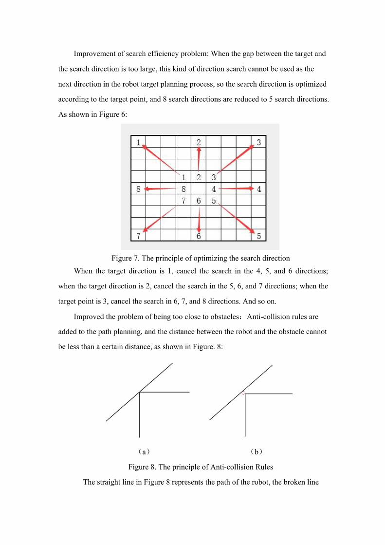
Improvement of search efficiency problem: When the gap between the target and
the search direction is too large, this kind of direction search cannot be used as the
next direction in the robot target planning process, so the search direction is optimized
according to the target point, and 8 search directions are reduced to 5 search directions.
As shown in Figure 6:
Figure 7. The principle of optimizing the search direction
When the target direction is 1, cancel the search in the 4, 5, and 6 directions;
when the target direction is 2, cancel the search in the 5, 6, and 7 directions; when the
target point is 3, cancel the search in 6, 7, and 8 directions. And so on.
Improved the problem of being too close to obstacles:Anti-collision rules are
added to the path planning, and the distance between the robot and the obstacle cannot
be less than a certain distance, as shown in Figure. 8:
(a) (b)
Figure 8. The principle of Anti-collision Rules
The straight line in Figure 8 represents the path of the robot, the broken line

R
represents the obstacle in the path planning, and the red circle represents the gap
between the robot and the obstacle. It can be seen in Figure 8 (a) that the distance
between the robot and the obstacle is not considered in the original route planning.
After adding the anti-collision rule, the separation distance between the robot and the
obstacle is increased, which reduces the probability of collision.
Improved route planning algorithm for long-distance scenes : In long-distance
scenes, the route that appears according to the original evaluation function is not the
optimal curve, so we change the original evaluation function to formula (9):
F (n) = g(n)+ (1+ r )* h(n) (9)
In the above formula (2), r represents the distance from the current point to the
target point, and R represents the distance from the starting point to the target point.
When the current point is far from the target point, the weight of the heuristic function
becomes important. When the distance becomes smaller, the weight of the heuristic
function gradually tends to 1, and will not fall into the local optimal solution.
Improve the curve that is not smooth:Improve the Floyd algorithm to optimize
the two-way smoothness of the path and remove redundant points. Optimization is
shown in Figure 7:
Figure 9. Improved Floyd algorithm to optimize route planning
It can be seen from Figure 9 that the improvement removes the blue node and its
corresponding route, which optimizes the path and shortens the distance of the route.
For the ant colony algorithm, the smoothness of the path is further improved. Combine
it with cubic spline curve. When path planning needs to pass corners, the curve
becomes smoother, reducing the distance of route planning. The optimization
method is shown in Figure 8:

(a) (b)
Figure 10. Improved ant colony algorithm for route optimization effect
The black square indicates the non-driving area, the white square indicates the
passable area, and the red line indicates the planned route. Figure 10(a) is before
optimization, Figure 10(b) is after optimization.
4.1.3 Ant Clony Optimization
The ant colony algorithm is to imitate the natural ant colony's process of finding
food from the nest. It can find the origin, go through a number of given demand points,
and finally return to the origin of the shortest path [6]. Expressed by formula (10):
(10)
It is a probabilistic algorithm used to find an optimal path. Ants secrete
pheromone when walking, and the concentration of pheromone changes with the
number of ants. In the end, the path with the most pheromone is regarded as the
shortest path. The information that inspires ants to move from a random direction to
the target point is called heuristic information, which is defined as formula (11):
(11)
Among them, i, j represent two points, and d(i, j) represents the Euclidean
distance between the two points. In the algorithm, the ant's choice of the next node is
based on the pheromone concentration and heuristic information of the i, j nodes on
the path, according to formula (12):
( )
( ) ( )
( ) ( )ïî
ïí
ìÎ
å= Î
other
Ajtt
t
tpijijAj
tijij
k
ij
0
baa
ba
ht
ht
k
,
allow,1
Î= jd ji
ijh

(12)
Among them, the pheromone released quantitatively during the movement of the ant
is the initial pheromone q0. Compare the pheromone q, if q>q0, select the pheromone
of the path after all ants complete one iteration after t time, then (t+1) seconds the
above path pheromone is updated as formula (13) and formula (14):
(13)
(14)
Since the pheromone volatilizes in the iterative process, use ρ to represent its
volatilization coefficient, and the interval range is (0, 1), Tij(t) represents the residual
concentration of pheromone in the path at time t. Q represents the fixed value of the
total content of pheromone, and Lk represents the optimal path length found by the
ants after traversal.
4.1.4 Annealing algorithm
The simulated annealing algorithm starts from the initial solution i and the initial
value t of the control parameter, and repeats the iteration of "generate a new solution
→ calculate the objective function difference → accept or discard" the current
solution. And gradually attenuate the value of t, so that the current solution when the
algorithm terminates is the approximate optimal solution obtained. The annealing
process is controlled by the cooling schedule, which includes the initial value t of the
control parameter and its attenuation factor Δt, the number of iterations L at each t
value, and the stop condition S.
The algorithm is shown in Figure 11:
( ) ( )
( )ïî
ïíì
>
£=
Î
b
k
ij
ijijAi
qqtp
qqttj
0maxargba ht
( ) ( ) ( )1,)1(1 +D+-=+ ttttijijijttrt
( )ïî
ïíì
=+D0
1, kL
Q
ij ttt

Figure 11. The overview of annealing algorithm
4.2 Experimental results and analysis

Figure 12. The effect of traditional A* algorithm
Figure 13. The effect of traditional A* algorithm combined with ant colony algorithm
Figure 14. The effect of traditional A* algorithm combined with annealing algorithm
Figure 15. The effect of improved A* algorithm combined with ant colony algorithm
Figure 16. The effect of improved A* algorithm combined with annealing algorithm

Choose a room of 104 square meters for experiment, as shown in Figure 12,
Figure 13, Figure 14, Figure 15 and Figure 16. Black squares represent obstacles. Red
lines represent routes of traditional A* algorithm and ant clony
algorithm,and blue lines represent paths of annealing algorithm.Figure 12 shows the
route obtained by the traditional A* algorithm. Figures 13 shows the route obtained by
the traditional A* algorithm combined with ant colony algorithm. Figure 14 shows the
route obtained by traditional A* algorithm combined with annealing algorithm. Figure
15 shows the route obtained by improved A* algorithm combined with ant colony
algorithm. Figure 16 shows the route obtained by improved A* algorithm combined
with annealing algorithm.
Table Ⅰ. Comparison of experimental results with different methods
Method Distance
Traditional A* algorithm
Traditional A* algorithm combined with
ant colony algorithm
Traditional A* algorithm combined with
annealing algorithm
Improved A* algorithm combined with
ant colony algorithm
Improved A* algorithm combined with
annealing algorithm
1254.0559
198.7696
185.5391
190.6579
179.9081
The following conclusions can be obtained from the table Ⅰ:
Compared with the traditional A* algorithm combined with the ant colony
algorithm and the improved A* algorithm combined with the ant colony algorithm,
the optimization effect of the path reached 4.08%. Compared with the traditional A*
algorithm combined with the annealing algorithm, the optimization effect of the
improved A* algorithm path combined with the annealing algorithm reaches 3.03%. It
can be seen that the improvement of the A* algorithm shows good performance.
Therefore, the improved A* algorithm combined with the annealing algorithm is
selected on the route planning module of the intelligent robot.

Figure 17. The effect of improved A* algorithm combined with annealing
algorithm of the real room
As shown in Figure 17, the experiment conducted by the intelligent robot of the
real room, through the experimental results. It can be seen that the route planning
module shows excellent results.
Further, in order to verify that the method can be widely applied to different
scenarios, we have verified the number of plants in different types of houses. After a
lot of experiments, the following table Ⅱ was obtained:
Table Ⅱ. Comparison of experimental results of different scenes
Area Number of plants Method
0-50 Square meters 1-3
Improved A* algorithm combined
with annealing algorithm
0-50 Square meters 3-6
Improved A* algorithm combined
with annealing algorithm
0-50 Square meters 6-9
Improved A* algorithm combined
with annealing algorithm
0-50 Square meters 9-12
Improved A* algorithm combined
with annealing algorithm
0-50 Square meters 12-15
Improved A* algorithm combined
with annealing algorithm
50-100 Square meters 1-3
Improved A* algorithm combined
with annealing algorithm
50-100 Square meters 3-6
Improved A* algorithm combined
with colony algorithm

50-100 Square meters 6-9
Improved A* algorithm combined
with annealing algorithm
50-100 Square meters 9-12
Improved A* algorithm combined
with annealing algorithm
50-100 Square meters 12-15
Improved A* algorithm combined
with annealing algorithm
100-150 Square meters 1-3
Traditional A* algorithm combined
with annealing algorithm
100-150 Square meters 3-6
Improved A* algorithm combined
with annealing algorithm
100-150 Square meters 6-9
Improved A* algorithm combined
with annealing algorithm
100-150 Square meters 9-12
Improved A* algorithm combined
with annealing algorithm
100-150 Square meters 12-15
Improved A* algorithm combined
with annealing algorithm
From Table Ⅱ, conclusions can be drawn through experimental results: The
improvement of A* algorithm is extensive and can be applied in most indoor
situations. The route planning module based on the improved A* algorithm combined
with the annealing algorithm shows excellent performance in the experiment.
5. Conclusion
For plant positioning and route planning in an unknown environment, the key
marker algorithm proposed in this article can be combined with route planning in
intelligent plant cultivation robots. In terms of path optimization, this thesis improves
the original shortcomings and drawbacks of the A* algorithm. The improved A*
algorithm is further combined with the ant colony algorithm and the annealing
algorithm. Further optimization of the paths has effectively solved the problems of
traditional A* algorithm, such as many turning points, large turning angles, and
feasible paths that are not the actual optimal paths. The key maker algorithm uses the

features learned by the deep convolutional neural network to detect plants. The type
and location information of plants can be directly obtained by absorbing and refining
characteristics. Make the key maker of the target plant and record the position in the
global coordinate system. The system proposed in this paper significantly improves
the efficiency of plant positioning and path planning. Aiming at the problems of
inconvenience in finding plants, low efficiency, and excessive influence by the
external environment, the intelligent plant cultivation robot shows excellent
performance. Finally, through a large number of experiments, the effectiveness and
advancement of the system are confirmed.
Reference:
[1] Acaccia, G. M., et al. "Mobile robots in greenhouse cultivation: inspection and
treatment of plants." Memories. Paper presented in 1st International Workshop on
Advances in Services Robotics. Bardolino, Italia. 2003.
[2] Usami H . Plant cultivation system in intelligent plant factory[J]. Journal of
Pesticide Science, 2012, 36(4):503-509.
[3] Andreasson H , Duckett T , Lilienthal A J . A minimalistic approach to
appearance-based visual SLAM. IEEE Trans. Robot. 24, 1-11[J]. IEEE Transactions
on Robotics, 2008, 24(5):991-1001.
[4] Kim A , Eustice R M . Active visual SLAM for robotic area coverage: Theory and
experiment[J]. The International Journal of Robotics Research, 2014,
34(4-5):457-475.
[5] Bosse M , Zlot R . Map Matching and Data Association for Large-Scale
Two-dimensional Laser Scan-based SLAM[J]. The International Journal of Robotics
Research, 2008, 27(6):667-691.
[6] Kamarudin K , Mamduh S , Shakaff A , et al. Performance Analysis of the
Microsoft Kinect Sensor for 2D Simultaneous Localization and Mapping (SLAM)
Techniques[J]. Sensors, 2014, 14(12):23365-87.
[7] Gkioxari G , Girshick R , Malik J . Contextual Action Recognition with R*CNN[J].
International Journal of Cancer Journal International Du Cancer, 2015,

40(1):1080-1088.
[8] Ren S , He K , Girshick R , et al. Faster R-CNN: Towards Real-Time Object
Detection with Region Proposal Networks[J]. IEEE Transactions on Pattern Analysis
and Machine Intelligence, 2015, 39(6).
[9] Liu W , Anguelov D , Erhan D , et al. SSD: Single Shot MultiBox Detector[C]//
European Conference on Computer Vision. Springer, Cham, 2016.
[10] Redmon J , Farhadi A . YOLOv3: An Incremental Improvement[J]. arXiv e-prints, 2018.
[11]Pezzuolo, Andrea, Guarino, et al. A Feasibility Study on the Use of a Structured
Light Depth-Camera for Three-Dimensional Body Measurements of Dairy Cows in
Free-Stall Barns[J]. Sensors, 2018.
[12]P. E. Hart, N. J. Nilsson, and B. Raphael. A formal basis for the heuristic
determination of minimum cost paths in graphs. IEEE Trans. Syst. Sci. and
Cybernetics, SSC-4(2):100-107, 1968
[13] Ma X , Chen Y , Bai G , et al. Path planning and task assignment of the
multi-AUVs system based on the hybrid bio-inspired SOM algorithm with neural
wave structure[J]. 2021.
[14] He T , Tong H . Remote sensing image classification based on adaptive ant colony
algorithm[J]. Arabian Journal of Geosciences, 2020, 13(14).
[15] Dorigo M , Caro G D , Gambardella L M . Ant Algorithms for Discrete
Optimization[J]. Artificial Life, 1999, 5(2):137-172.
[16] Lundy M , Mees A . Convergence of an annealing algorithm[J]. Mathematical
Programming, 1986, 34(1):111-124.
[17] Brunn P . Robot collision avoidance[J]. Industrial Robot, 1996, 23(1):27-33.
[18]Floyd R W . Algorithm 97, Shortest Path Algorithms[J]. Communications of the
ACM, 1962, 5(6):345.

Figures
Figure 1
Intelligent plant cultivation robot

Figure 2
System overview
Figure 3
The global map adjusted by multiple submaps

Figure 4
Reconstructed map with key marks
Figure 5

The overview of key maker algorithm
Figure 6
The overview of the A* algorithm

Figure 7
The principle of optimizing the search direction

Figure 8
The principle of Anti-collision Rules
Figure 9
Improved Floyd algorithm to optimize route planning

Figure 10
Improved ant colony algorithm for route optimization effect

Figure 11
The overview of annealing algorithm

Figure 12
The effect of traditional A* algorithm
Figure 13
The effect of traditional A* algorithm combined with ant colony algorithm

Figure 14
The effect of traditional A* algorithm combined with annealing algorithm
Figure 15
The effect of improved A* algorithm combined with ant colony algorithm
Figure 16
The effect of improved A* algorithm combined with annealing algorithm
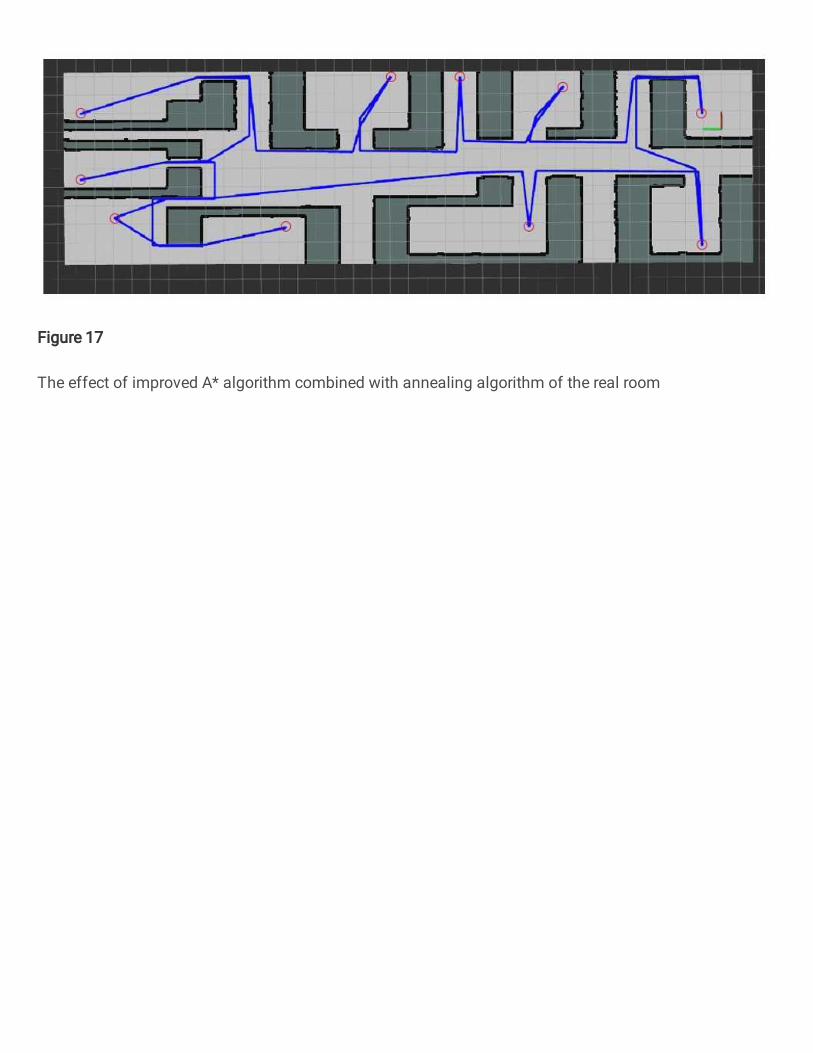
Figure 17
The effect of improved A* algorithm combined with annealing algorithm of the real room