Intelli MAC Layer Protocol for Cognitive Radio Networks

Rochester Institute of TechnologyRIT Scholar Works

Theses Thesis/Dissertation Collections

7-2009

Intelli MAC Layer Protocol for Cognitive RadioNetworksRahul K. Patibandla

Follow this and additional works at: http://scholarworks.rit.edu/theses

This Thesis is brought to you for free and open access by the Thesis/Dissertation Collections at RIT Scholar Works. It has been accepted for inclusionin Theses by an authorized administrator of RIT Scholar Works. For more information, please contact [email protected].

Recommended CitationPatibandla, Rahul K., "Intelli MAC Layer Protocol for Cognitive Radio Networks" (2009). Thesis. Rochester Institute of Technology.Accessed from

http://scholarworks.rit.edu?utm_source=scholarworks.rit.edu%2Ftheses%2F8714&utm_medium=PDF&utm_campaign=PDFCoverPages

http://scholarworks.rit.edu/theses?utm_source=scholarworks.rit.edu%2Ftheses%2F8714&utm_medium=PDF&utm_campaign=PDFCoverPages

http://scholarworks.rit.edu/etd_collections?utm_source=scholarworks.rit.edu%2Ftheses%2F8714&utm_medium=PDF&utm_campaign=PDFCoverPages

http://scholarworks.rit.edu/theses?utm_source=scholarworks.rit.edu%2Ftheses%2F8714&utm_medium=PDF&utm_campaign=PDFCoverPages

http://scholarworks.rit.edu/theses/8714?utm_source=scholarworks.rit.edu%2Ftheses%2F8714&utm_medium=PDF&utm_campaign=PDFCoverPages

mailto:[email protected]

Intelli MAC Layer Protocol for Cognitive Radio Networks

by

Rahul K Patibandla

A Thesis Submitted in Partial Fulfillment of the Requirements for the Degree of

Master of Science in Computer Engineering

Supervised by

Dr. Andres Kwasinski

Department of Computer Engineering

Kate Gleason College of Engineering

Rochester Institute of Technology

Rochester, NY

July 2009

ii

Dedication

In Loving Memory of My Dad…Whom I Miss So Much

iii

Acknowledgements

I would like to take this opportunity to thank my advisor,

Dr. Andres Kwasinski who has mentored and guided me during the course of this thesis.

He is a good friend and a great guide to me throughout the thesis. He has provided me

with lot of confidence, encouragement and good ideas that helped me to work towards

the completion of the thesis. His knowledge base is formidable one and I hope to make

the maximum utilization of such effective guidance. His inspiring guidance enabled me

give my best to the thesis. His valuable tips at the right times enabled me to progress in

the right direction. Without his help and knowledge none of this thesis would have been

possible.

My deep and sincere thanks to the department head

Dr. Andreas Savakis for his constant encouragement and motivation for completing my

thesis.

I also thank Dr. Pratapa V Reddy and Dr. Direesha Kudithipudi for

being a part of my committee and provided me their continuous support and

encouragement in making this research work possible. Their able and inspiring guidance

shall go fathoms unforeseen into the efforts for completing my thesis. Also I would like

to thank all my friends and my colleagues who have provided me with their feedback and

valuable suggestions throughout the duration of this work.

iv

Abstract

According to the FCC (Federal Communications Commission) [11], the

utilization of the spectrum has been increasing rapidly over a wide range of frequency

bands. There are various reasons that cause this dynamic growth. One reason is increase

in network capacity. Another reason is increase in mobile services needed to carry over

the spectrum. In order to overcome the shortage of spectrum due to increased usage,

Cognitive Radio (CR) technology has been introduced. Cognitive Radios can utilize idle

spectrum holes that are not occupied by the Primary Users (PUs) for performing

temporary wireless communication tasks. PUs are licensed users which own and have

access to certain spectrum bands. Challenging issues that need to be addressed by the

CRs are spectrum sensing, spectrum sharing, spectrum management and spectrum

mobility.

The main contribution of this thesis is to design a new MAC layer protocol in

order to determine the behavior of Secondary Users (SUs) based on PUs transmission

history while taking into account both PUs and SUs. SUs are non licensed users which

transmit only on those spectrum bands that are unutilized by the PUs. SUs usually

observe the activity of PUs on spectrum bands. This new protocol allows the CR nodes to

sense, share and manage access of the nodes to the spectrum. This protocol prevents any

damage caused by SUs to the PUs transmission. Also, the new MAC protocol will

negotiate the spectrum by assisting the CRs to identify the underutilized spectrum based

on channel conditions such as channel throughput, channel data rate, channel score,

channel utilization and packet error rate (PER). The Intelli MAC layer protocol measures

transmission time among PUs and reduces channel sensing time for SUs. For managing

v

the entire network, this protocol uses the concept of Harmonious Channel (HC). This

protocol uses multiple half duplex transceivers for carrying data communication among

users.

vi

Table of Contents

Acknowledgements .............................................................................................. iii

Abstract….. ........................................................................................................... iv

Table of Contents ................................................................................................ vii

List of Figures ....................................................................................................... ix

List of Tables ......................................................................................................... x

Glossary…. ........................................................................................................... xi

Chapter 1 Introduction ....................................................................................... 1

1.1. Simplex, Half and Full Duplex Transceivers .......................................... 1

1.2. Cognitive Radios ..................................................................................... 2

1.3. Cognitive Radios Classification .............................................................. 5

1.4. Spectrum Sensing in CRNs ..................................................................... 6

1.5. Thesis Contributions ............................................................................... 6

1.6. Thesis Outline ......................................................................................... 8

Chapter 2 Background ........................................................................................ 9

2.1. Existing CRs MAC layer protocols ........................................................ 9

2.1.1 Opportunistic Cognitive MAC protocol (OC-MAC) .............................. 9

2.1.2 Dynamic open spectrum sharing MAC protocol (DOSS) .................... 10

2.1.3 Common Spectrum Coordination Channel Protocol (CSCC) .............. 13

2.1.4 Distributed channel assignment protocol (DCA) .................................. 14

2.1.5 Slotted Seeded Channel hopping algorithm (SSCH) ............................ 15

2.2. Spectrum Sharing in MAC Layer ......................................................... 16

2.3. CR Hidden and Exposed Terminal Problem ......................................... 18

Chapter 3 Proposed MAC Protocol ................................................................. 22

3.1. Usage of Multiple Half Duplex Transceivers ....................................... 22

3.1.1 In-band and Out-of-band Sensing ........................................................ 24

3.2. Channel Selection ................................................................................. 25

3.3. Channel Utilization ............................................................................... 26

3.4. Channel Goodput .................................................................................. 26

3.5. Channel Slot (Predicted white space duration) ..................................... 28

3.5.1 Channel Scanning and Sending ............................................................. 29

3.6. Channel Score ....................................................................................... 31

3.7. Channel State Table .............................................................................. 33

vii

3.8. Harmonious Channel (HC) ................................................................... 35

3.8.1 HC Switching ....................................................................................... 36

3.8.2 HC Selection ......................................................................................... 37

3.8.3 PU Notification ..................................................................................... 37

3.8.4 PU Detection Recovery ......................................................................... 37

3.9. Performance Evaluation ........................................................................ 38

3.9.1 Channel Utilization ............................................................................... 39

3.9.2 Channel Goodput ................................................................................... 42

3.9.3 Channel Slot ......................................................................................... 44

3.9.4 Channel Score ....................................................................................... 46

Chapter 4 NS-2 (Network Simulator) .............................................................. 49

4.1. C++/Tcl ................................................................................................. 49

4.2. NS-2 Installation Instructions ............................................................... 50

4.2.1 NS-2 installation on UNIX/LINUX Machine ...................................... 50

4.2.2 NS-2 installation on Windows Machine ............................................... 52

Chapter 5 Conclusions and Future Work ....................................................... 54

5.1. Future Work .......................................................................................... 54

Chapter 6 Bibliography ..................................................................................... 56

Chapter 7 Appendix.......................................................................................... 58

viii

List of Figures

Figure 1. Hidden Terminal Problem ..................................................................... 18

Figure 2. Hidden Terminal Problem Solution....................................................... 19

Figure 3. Exposed Terminal Problem ................................................................... 20

Figure 4. Block diagram of half duplex transceivers ( T1 and T2) ....................... 24

Figure 5. Channel Slot Duration ........................................................................... 29

Figure 6. Channel scanning scheme...................................................................... 30

Figure 7. Channel Utilization in case of Intelli MAC Protocol ............................ 40

Figure 8. Channel Utilization in case of OC-MAC protocol ................................ 40

Figure 9. Channel Utilization (Intelli MAC Layer vs. OC-MAC) ....................... 41

Figure 10. Goodput vs. Channel (Intelli MAC Layer protocol) ........................... 42

Figure 11. Goodput vs. Channel (OC-MAC protocol) ......................................... 43

Figure 12. Channel Goodput (Intelli MAC Layer vs. OC-MAC)......................... 43

Figure 13. Channel slot in case of Intelli MAC Protocol ..................................... 44

Figure 14. Channel slot in case of OC-MAC Protocol ......................................... 45

Figure 15. Channel Score in case of OC-MAC Protocol ...................................... 46

Figure 16. Channel Score in case of Intelli MAC Protocol .................................. 47

ix

List of Tables

Table 1. Three channels with channel utilization and channel score values .. ..... ………34

Table 2. Data rates and PER for 6 channels……………………………………………..39

Table 3. Three channels with channel goodput, channel utilization, data rate, PER,

channel score and channel slot values. ............................................................ .47

x

Glossary

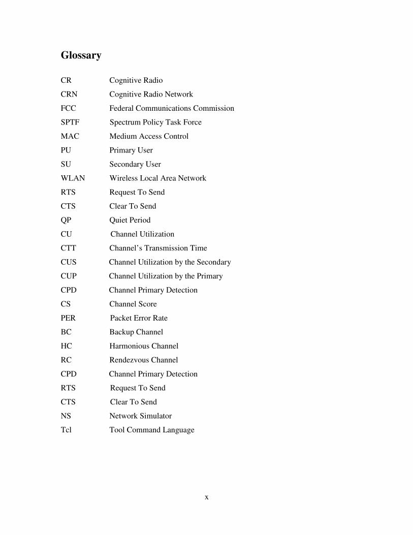
CR Cognitive Radio

CRN Cognitive Radio Network

FCC Federal Communications Commission

SPTF Spectrum Policy Task Force

MAC Medium Access Control

PU Primary User

SU Secondary User

WLAN Wireless Local Area Network

RTS Request To Send

CTS Clear To Send

QP Quiet Period

CU Channel Utilization

CTT Channel’s Transmission Time

CUS Channel Utilization by the Secondary

CUP Channel Utilization by the Primary

CPD Channel Primary Detection

CS Channel Score

PER Packet Error Rate

BC Backup Channel

HC Harmonious Channel

RC Rendezvous Channel

CPD Channel Primary Detection

RTS Request To Send

CTS Clear To Send

NS Network Simulator

Tcl Tool Command Language

1

Chapter 1 Introduction

1.1. Simplex, Half and Full Duplex Transceivers

A given transmission on a communication channel between transmitter and

receiver can occur in several different ways. The transmission is characterized by the

direction of data exchange, transmission mode (number of bits sent simultaneously) and

synchronization between transmitter and receiver. Three different types of transceivers

may be used to transmit data. They are simplex, half and full duplex transceivers. The

following explanation gives a basic idea of different transceivers functionality.

Simplex Transceivers:

1. Data is always transmitted in one direction.

2. These transmitters are not often used because it is not possible to send back

error or control signal to the transmitting end.

3. Examples of simplex transceivers are television and radio transceivers.

Half Duplex Transceivers:

1. Data is sent and received in both directions but not at the same time.

2. One end transmits at a time and the other end receives.

3. For these transceivers, it is possible to perform error detection and request the

sender to retransmit information that arrived corrupted.

4. Examples of half duplex transceivers are talkback radio and CB radio.

2

Full Duplex Transceivers:

1. Data is sent and received in both directions simultaneously.

2. There is no need for the transceivers to switch from transmit to receive mode

like in the case of half duplex transceivers.

3. Examples of full duplex transceivers are cable connection and telephone.

1.2. Cognitive Radios

The concept of Cognitive Radios has been defined as “the point in which wireless

personal digital assistants (PDAs) and the related networks are sufficiently

computationally intelligent about radio resources and related computer-to-computer

communications to detect user communications needs as a function of use context and

to provide radio resources and wireless services most appropriate to those needs” [4].

Many regulatory bodies like the Federal Communications Commission (FCC)

in the United States observed that the radio spectrum is inefficiently utilized [11].

Wireless communication and its applications are witnessing an explosive growth

today. It has been predicted [18] that about 55% of all users will access the internet

wirelessly. In wireless systems, spectrum is a very costly and limited resource, which

has to be used intelligently. Many researchers point out that spectrum identification

and spectrum management are bigger problems in reality than spectrum

availability. Due to logistical issues, it is difficult to centrally control spectrum

distribution. In fact, if one identifies a segment of the Radio Frequency (RF)

spectrum, it will notice that some frequency bands are overcrowded but some others

are virtually empty [17]. Cognitive Radio technology has been introduced to overcome

the shortage of spectrum usage [2]. Cognitive Radios can sense the environment

3

around them and can alter the operating frequencies, power and modulation

techniques in order to use the spectrum efficiently[4].

Cognitive Radios (CR) have the following features.

a) Cognitive Radios are able to identify and detect the channel in the

available band that is not being used and tune to that particular channel.

b) After identifying the channel, they establish the network connection and

operate in that particular channel.

c) Obtaining the best throughput is the primary aspect for any type of data

transmission system. CRs use better bandwidth for efficient data transmission

and also error control and correction schemes to obtain the best throughput.

d) Cognitive Radios can switch to another empty channel.

With the help of the CR techniques, the entire wireless spectrum is used for

communication by cognitive radio networks. They also reduce the interference

among the users.

A CR is designed to be aware of the changes in its surroundings. This

makes spectrum sensing an important requirement for the realization of CR networks

[19]. Spectrum sensing enables CR users to adapt to the radio environment by

determining currently the unused spectrum portions. The unused portions are known as

spectrum holes [19]. Typically a CRN needs to identify two distinct classes of spectrum

holes [12]: global holes and local holes. Global holes are the unused frequency bands

which can be detected by the users in the entire network or large geographical area. For

example, the geographical area in the case of a television transmitter is so large that the

4

entire network will experience a similar spectrum sensing measurement. The CRNs use

holes identified in these bands for global signaling and data messaging. Local holes on

the other hand are unused frequency bands that can be identified by users in a small

geographical area but not be detected by the users in other areas. These frequencies are

used by local area networks. The CRNs use holes identified in these bands for local

control signaling and data messaging.

IEEE 802.11[15] is the set of standards for wireless local area network (WLAN),

developed by the IEEE LAN/MAN (Local Area Network/Metropolitan Area Network)

Standards Committee. The IEEE 802.11 standard provides network bandwidth up to

54 Mbps. In the 2.4 GHz band, it provides a network bandwidth of 1 to 2 Mbps.

Hence the IEEE 802.11 standard is too slow for most of the wireless

applications. Recognizing the critical needs to support higher data transmission

rates, the IEEE 802.11b standard with transmission rate of 11Mbps has been

introduced. The IEEE 802.11b is also referred to as the 802.11 High Rate or Wi-Fi.

The IEEE 802.11b provides 11Mbps transmission with a fallback to 1, 2, 5.5 and

7Mbps. Hence each user can operate with a different data rate. The IEEE 802.11b

is an amendment to the original IEEE 802.11 standard. The advantages of 802.11b

are lowest cost, higher performance and throughput and good signal range [20].

Also they cannot be easily obstructed. The disadvantages of 802.11b are slow maximum

speed and interference as compared to the Ethernet.

5

1.3. Cognitive Radios Classification

The CRs can be classified into various types. They are Full CR, Spectrum Sensing CR,

Licensed Band CR and Unlicensed Band CR [4].

1. Full CR takes every parameter that is being observed by the wireless node

or network into account and then makes decisions on the change in

the transmission or reception mode.

2. Spectrum sensing CR senses the entire spectrum and detects the part

of the spectrum that is left unused and then shares this part of the spectrum

with the other users without causing any interference to the PUs.

3. Licensed band CR uses portion of the spectrum that is particularly meant for

the licensed user access. The licensed band CR primarily checks for the

available PU on the particular channel of the spectrum. If the PU is

active, then it switches to another channel and if the PU is not

active, then it gives access to the unlicensed user (SU) and monitors

the entire channel for the PU. An example for the Licensed Band CR is

IEEE 802.22 [4].

4. Unlicensed Band CR uses the unlicensed parts of the spectrum that are

available. Therefore, there is no need for the CR to sense the entire spectrum

till the SUs use the channel. Example for the Unlicensed Band CR is

IEEE 802.19 [4].

6

1.4. Spectrum Sensing in CRNs

The Spectrum Policy Task Force (SPTF) report released

by the FCC [11] acknowledged the existence of unused spectrum in the

licensed bands. The licensed bands are exclusively reserved for use by the primary

license holders (primary users). The spectrum usage indicates that many licensed

spectrum bands remain relatively unused for most of the time. The FCC has

determined that in some locations at certain times of the day, up to 70% of the

allocated spectrum may be unused, even though it is officially licensed to a

specific user [12]. Cognitive radio technology plays a major role in this FCC

policy because there exists an opportunity for these radios to use these licensed bands

when primary users are absent and hence improve the overall spectrum usage

efficiently.

Users with the cognitive capability can sense the radio

spectrum environment within their operating range to detect the channels that are

not occupied by licensed users or primary users.

1.5. Thesis Contributions

The main contribution of this thesis is to design a new MAC layer protocol

known as “Intelli MAC” that identifies the channels to be used by SUs very

efficiently. Intelli MAC layer protocol uses multiple half duplex transceivers

for carrying the communication among users. In case of the Intelli MAC layer

protocol, SUs will not interfere or cause any damage to the PUs

transmission. During the time that PUs are transmitting, the SUs perform

7

spectrum sensing to identify the channel to carry on with their communication.

Other existing protocols perform certain functions like spectrum allocation,

spectrum access and spectrum mobility. SUs transmission will be interrupted completely

in case of PUs presence on the channel. SUs have to vacate the channel even in case of

non transmitting PUs. The channel selection for communication purposes is arbitrary and

not based on a particular selection criteria like in the case of Intelli MAC layer protocol.

The CR mechanism used in the Intelli MAC protocol can be applied to either SUs

or PUs. Since PUs are the licensed users and can access the spectrum at any point of

time, the CR mechanism is mostly applied to SUs. Using the CR mechanism, SUs are

able to sense and manage the available spectrum. SUs can detect the presence of PUs

currently accessing the channel and also detect PUs transmission. After detecting PUs

transmission, the SUs can move into another channel for communication. Hence Intelli

MAC layer protocol can prevent any damage that can be caused to the transmission from

PUs by the SUs.

In this thesis, the new proposed MAC protocol negotiates the spectrum following

a channel selection criteria based on channel score, channel utilization, channel state table

and predicted white space duration. With the help of these parameters, the CR device is

able to identify the portion of the spectrum which is underutilized and thereby providing

access to the SUs without causing any interference to the PUs. Also this protocol is able

to select different channels based on Packet Error Rate (PER). PER can be used to

differentiate one channel from the other and also to have an idea about how much data a

channel can deliver.

8

The Intelli MAC layer protocol uses the Harmonious Channel (HC) concept. HC

is used to manage the entire network. It is used to carry the coordination among the users.

Since all the SUs have to visit this HC for resynchronization purposes, it is used for

maintaining the coordination among users.

1.6. Thesis Outline

Chapter 2 provides a background on previously developed MAC protocols for CRNs. It

also details some MAC layer Spectrum Sharing issues and impact of the channels.

Chapter 3 introduces the proposed Intelli MAC layer protocol. This chapter provides a

detailed explanation of the concept of Harmonious Channel. Also this chapter details the

simulation results and compares the performance of Intelli MAC layer protocol with the

other existing protocol (Opportunistic Cognitive MAC protocol). Chapter 4 describes the

software NS2 used for the simulations in this thesis. Finally, Chapter 5 provides a

concluding summary of this thesis and comments for future research work.

9

Chapter 2 Background

2.1. Existing CRs MAC layer protocols

The performance of wireless networks is improved by introducing various

Medium Access Control (MAC) protocols. MAC layer protocols in CRNs handle

spectrum sensing, spectrum access scheduling and spectrum sharing[4].

MAC layer protocols for CRNs are capable to handle dynamic access over multiple

channels, capable to coordinate with other spectrum sharing CRs and capable to reason

using intelligent decision algorithms [4]. In this chapter we provide survey of several

previously proposed CRNs MAC schemes. They are the Opportunistic Cognitive

MAC (OC-MAC) protocol [1], the Dynamic Open Spectrum Sharing (DOSS)

protocol [5], the Common Spectrum Coordination Channel (CSCC) protocol [6],

the Distributed Channel Assignment (DCA) protocol [7] and the Slotted Seeded

Channel Hopping (SSCH) protocol [8].

2.1.1 Opportunistic Cognitive MAC protocol (OC-MAC)

The Opportunistic Cognitive MAC (OC-MAC) protocol is a decentralized,

asynchronized and connection-prone MAC protocol [1]. This protocol focuses on

transmission issues over multiple channels and effective connection establishment.

A handshaking process and channel selection mechanisms are used in OC-MAC [1].

This protocol predicts the length of spectrum holes during the spectrum vacancy. It

addresses three problems in an integrated manner [1] channel selection, medium access

and collision avoidance.

10

Advantages

1.) It is flexible and can be deployed fast.

2.) Avoids producing fatal damage to the licensed users.

3.) Improves low-throughput of the primary network.

Disadvantages

1.) No coordination among users in the network.

2.) It does not support network management.

3.) It does not consider non-licensed users (SUs) behavior during licensed users

(PUs) transmission.

Applications

1.) Mainly used in WLANs (Wireless Local Area Networks).

2.1.2 Dynamic open spectrum sharing MAC protocol (DOSS)

The dynamic open spectrum sharing (DOSS) algorithm [5] divided the MAC

protocol of CRNs into five steps [4]. They are (a) detecting the presence of a PU,

(b) setting up three frequency bands (busy tone band, control channel band and

data band ), (c) mapping the spectrum, (d) negotiating with the spectrum and

(e) transmitting the data.

(a) Detecting the presence of PUs:

The SUs make use of the spectrum only when the PUs are not accessing it.

This involves frequent messages exchange among neighbors to reach a global

view of channel availability information [4], [5].

11

(b) Setting up three operational frequency bands:

The control channel is mainly used to help the radio receiver to identify the

particular channel in which they can operate. After identifying the particular

channel in which the radio can operate the control channel can use the

data band to start transmitting data [4], [5].

(c) Spectrum Mapping:

The spectrum mapping is used to establish a one-to-one mapping between

different busy tones and the data channels [5]. With the spectrum mapping

the receiver can set a busy tone on the portion of the spectrum in which it

is receiving the information, and informs the neighbors about the spectrum that

is currently using. By sharing the spectrum usage information, the

neighbors will avoid interfering by stopping sending their data over the used

spectrum part [4], [5].

(d) Spectrum Negotiation:

In this step, the sender and the receiver negotiate on a particular channel for the

data transmission. In the process of negotiation, initially the nodes sense the

spectrum and identify the channel availability. After identifying the channel,

the sender sends a “REQ” packet to the receiver. This REQ packet has the

information about the channel parameters. After receiving the REQ packet the

receiver checks with its own available channels, and picks the common

channel that is available to both the sender and the receiver. The receiver then

sends back a “REQ_ACK” packet indicating the choice of channel for

communication. After receiving the REQ_ACK packet from the receiver, the

12

sender identifies that the channel is available for transmission and starts the

data transmission [4], [5].

(e) Data Transmission:

The sender sends a “DATA” packet to the receiver. The receiver

acknowledges the sender with a “DATA_ACK” packet only after it

correctly receives the “DATA” packet. The sender realizes that the

transmission is successful only after it receives the “DATA_ACK” packet. If

the sender does not receive the “DATA_ACK” packet from the receiver, it

assumes that the transmission was unsuccessful and sends the DATA packet

again [4], [5].

Advantages

1.) It does not use fixed spectrum allocation.

2.) Prevents hidden and exposed terminal problems.

3.) Supports unicast and multicast.

4.) It is scalable and provides efficient real time spectrum allocation.

Disadvantages

1.) Requires multiple radio transmitters and receivers.

2.) Increases the device cost.

Applications

1.) Mainly used in wireless ad hoc networks operating over the spectrum.

13

2.1.3 Common Spectrum Coordination Channel Protocol (CSCC)

Another CR MAC scheme is called Common Spectrum Coordination Channel

Protocol (CSCC) [6]. In the CSCC all the users share a common control channel for

spectrum coordination purposes. Control information is exchanged using a narrow

band radio. All the users should periodically broadcast a request over the entire

spectrum whenever they intend to use the spectrum [4]. CSCC provides access to

those users who have a request for accessing the spectrum. Other users will remain

idle and not transmit any information [4], [6].

Advantages

1.) Allows flexibility among the spectrum sharing procedures.

2.) Advanced power control and multi hop routing procedures can be

implemented.

3.) The terminal start up procedures with the network can be avoided when

the user enters a new physical area.

4.) Collaborative spectrum usage can be used in this protocol.

5.) This protocol has multi-hop routing capabilities.

6.) It is scalable and an efficient real time spectrum allocation protocol.

Disadvantages

1.) This protocol causes the control channel saturation problem.

2.) It cannot handle hidden and exposed terminal problems.

3.) It cannot limit the traffic going through the control channel.

4.) It does not support multicast communications.

14

Applications

1.) Used for coordinating radio devices in unlicensed bands.

2.1.4 Distributed channel assignment protocol (DCA)

According to the distributed channel assignment protocol (DCA) [7] all users on the

network share one way handshake signal for data transmission. The transmitter and

the receiver of the SUs stops their transmission and reception upon identifying

the PU. In this protocol all the users use two antennas [7]. One antenna is used for

determining the traffic on the channel and the other is used for the spectrum sensing

and data transmission and data reception on the channel [4], [7].

Advantages

1.) It is a peer-to-peer cognitive radio network protocol.

2.) Negotiation takes place among two nodes only.

3.) All nodes use one way handshake for the information exchange.

Disadvantages

1.) There are restrictions on the channel assignment due to hardware

configurations.

2.) Potential inefficiency among the channel assignment.

Applications

1.) Used for wireless emergency communication networks.

15

2.1.5 Slotted Seeded Channel hopping algorithm (SSCH)

The users in this protocol share pseudo random codes for accessing the medium in a

time slotted manner [8]. Each user switches across the multiple channels so that

there is a significant increase in the network capacity. SSCH is a distributed

protocol. Synchronization is not required among the users in the network. Slot is

defined as the time that the user spends on the particular channel [4]. A longer

slot time will decrease the channel switching overhead but further increases the delay

among the packets. According to the slot time, user determines the list of the

channels to switch [4], [8].

Advantages

1.) The capacity of the ad-hoc wireless multi-hop networks is significantly improved.

2.) This protocol uses a single radio and does not use a dedicated control channel.

3.) This protocol works in both single-hop and multi-hop environment.

Disadvantages

1.) This protocol introduces long transmission delay.

2.) Communication overhead is significant for the short flows.

Applications

1.) Used for increasing the capacity of IEEE 802.11 networks by using frequency

diversity.

16

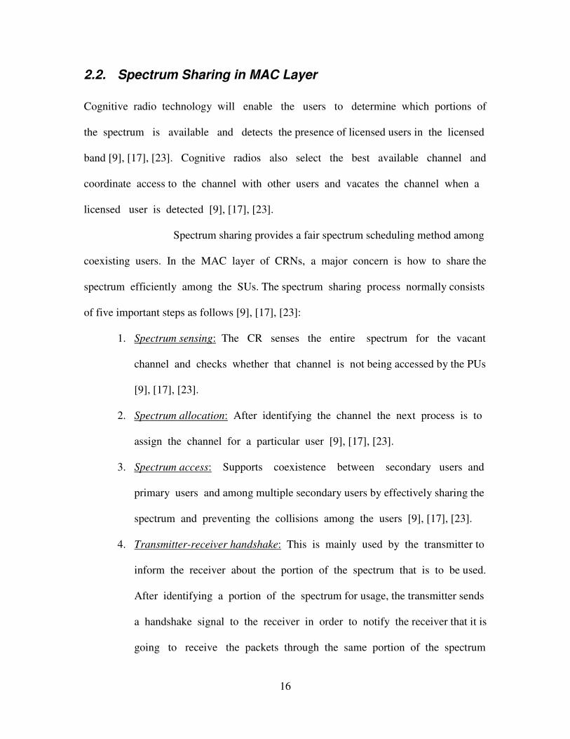
2.2. Spectrum Sharing in MAC Layer

Cognitive radio technology will enable the users to determine which portions of

the spectrum is available and detects the presence of licensed users in the licensed

band [9], [17], [23]. Cognitive radios also select the best available channel and

coordinate access to the channel with other users and vacates the channel when a

licensed user is detected [9], [17], [23].

Spectrum sharing provides a fair spectrum scheduling method among

coexisting users. In the MAC layer of CRNs, a major concern is how to share the

spectrum efficiently among the SUs. The spectrum sharing process normally consists

of five important steps as follows [9], [17], [23]:

1. Spectrum sensing: The CR senses the entire spectrum for the vacant

channel and checks whether that channel is not being accessed by the PUs

[9], [17], [23].

2. Spectrum allocation: After identifying the channel the next process is to

assign the channel for a particular user [9], [17], [23].

3. Spectrum access: Supports coexistence between secondary users and

primary users and among multiple secondary users by effectively sharing the

spectrum and preventing the collisions among the users [9], [17], [23].

4. Transmitter-receiver handshake: This is mainly used by the transmitter to

inform the receiver about the portion of the spectrum that is to be used.

After identifying a portion of the spectrum for usage, the transmitter sends

a handshake signal to the receiver in order to notify the receiver that it is

going to receive the packets through the same portion of the spectrum

17

[9], [17], [23].

5. Spectrum mobility: When a PU starts to accessing a portion of the

spectrum which is under use by the SUs, the SU should vacate that portion

and move to the other vacant portion of the spectrum while maintaining

the communication without any interruption [9], [17], [23].

In Dynamic Open Spectrum Sharing protocol [5], three different frequency bands

have been proposed in this protocol. They are data band, control channel, and busy tone

band [5]. The data band is mainly used for transferring the data from one point to the

other. The control channel can be regarded as the logic channel which is mainly used to

carry the network information instead of the actual voice or data messages that are

transmitted over the network. In the control channel band initially the sender

sends a request packet to the particular receiver . The request packet contains

the information about the channels of the sender. After the receiver receives

the request packet from the sender, then it compares the received

channels information with its own channels information. After comparing the

channels information, the receiver picks the channel that is common to

both the sender and the receiver and then sends an acknowledgement packet

to the sender [4], [5]. This acknowledgement packet has the information about

the channel that is common to both. After sending the acknowledgement

packet, the receiver turns on the busy tone over the channel that has been

picked as common to both the sender and the receiver and it informs the other

neighbors not to send the data over the same common channel as this channel is

allotted to a particular user (sender).

18

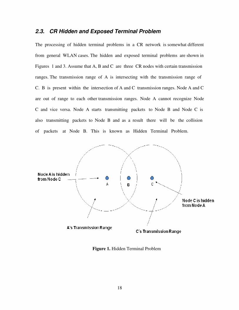
2.3. CR Hidden and Exposed Terminal Problem

The processing of hidden terminal problems in a CR network is somewhat different

from general WLAN cases. The hidden and exposed terminal problems are shown in

Figures 1 and 3. Assume that A, B and C are three CR nodes with certain transmission

ranges. The transmission range of A is intersecting with the transmission range of

C. B is present within the intersection of A and C transmission ranges. Node A and C

are out of range to each other transmission ranges. Node A cannot recognize Node

C and vice versa. Node A starts transmitting packets to Node B and Node C is

also transmitting packets to Node B and as a result there will be the collision

of packets at Node B. This is known as Hidden Terminal Problem.

Figure 1. Hidden Terminal Problem

19

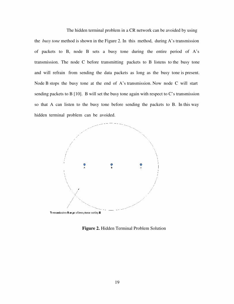
The hidden terminal problem in a CR network can be avoided by using

the busy tone method is shown in the Figure 2. In this method, during A’s transmission

of packets to B, node B sets a busy tone during the entire period of A’s

transmission. The node C before transmitting packets to B listens to the busy tone

and will refrain from sending the data packets as long as the busy tone is present.

Node B stops the busy tone at the end of A’s transmission. Now node C will start

sending packets to B [10]. B will set the busy tone again with respect to C’s transmission

so that A can listen to the busy tone before sending the packets to B. In this way

hidden terminal problem can be avoided.

Figure 2. Hidden Terminal Problem Solution

20

In the RTS/CTS mechanism one of the primary

issues in wireless networks are packet collisions due to exposed nodes. Therefore

in medium access schemes a mechanism known as RTS-CTS handshake is

considered to be essential for mitigating the effects of exposed nodes. RTS-CTS

mechanism prevents packet collisions by prohibiting nodes from transmitting [4].

The exposed terminal problem is shown in Figure 3. Assume that nodes A, B, C

and D are four CR nodes. Nodes A and D are out of range of each other and cannot listen

to each other transmission. Nodes B and C are within the range of each other and can

listen to each other transmission. Now, if a transmission from B to A is taking place,

node C is prevented from transmitting to node D as it determines after carrier sense that it

will interfere with the transmission by its neighbor B. According to the carrier sense, the

transmitting node listens for a carrier wave before trying to send. But node D could still

receive the data from node C without suffering from interference because it is out of

range from node A. This is known as exposed terminal problem [4].

Figure 3. Exposed Terminal Problem

21

The exposed terminal problem can be avoided using RTS/CTS mechanism. Node B

sends an RTS packet to node A. When node C hears the RTS but not the CTS from

the neighboring node B, then it assumes that B is an exposed node to D and

transmits RTS packet to node D.

Some problems still persist with the busy tone solution.

a) First, there is a need for new channels. One channel is used for transmitting and

receiving the data and the other is used for setting up the busy tone for

preventing the hidden and exposed terminal problems [4]. This result in

the expansion of the spectrum, i.e., more spectrum is used, and more

hardware is required for maintaining the additional channels.

b) Second, collisions still persist when the transmission range of the data channel

is greater than that of the busy tone band.

c) Third, when the busy tone band has larger transmission range than the data

channel, some of the data transmission will be suppressed [4].

22

Chapter 3 Proposed MAC Protocol

In Cognitive Radio Networks, Medium Access Control (MAC) protocols

identify the available spectrum resource through spectrum sensing. They decide on the

optimal sensing and transmission times and coordinate with the other users for

spectrum access. The Intelli MAC layer protocol allows the CR nodes to sense, share,

manage and also provides mobility to the nodes among the spectrum.

The Intelli MAC layer protocol negotiates the spectrum by assisting the CRs to

identify the underutilized spectrum using a channel selection criteria. The

channel selection criteria is based on properties such as channel score,

channel utilization, channel throughput, channel data rate and packet error rate.

With these properties, a better channel for transmitting or receiving data can

be selected. The hidden and exposed terminal problems can be prevented by

setting up a busy tone among group of channels.

3.1. Usage of Multiple Half Duplex Transceivers

A half duplex transceiver is used for communication in both directions, but only

one direction at a time. We assume the transceiver is able to switch the channels

dynamically due to the half duplex nature of the transceiver, and that the SUs can only

transmit or listen on one channel at a time. According to the FCC [11], usage of spectrum

is mainly based upon the single interface model. In the case of a single interface, each

node is equipped with one transceiver in the network. When a host is receiving on a

particular channel from the sender, it cannot hear the communication taking place on the

other channel. Due to packet collisions, single transceivers face problems such as reduced

23

throughput, packet loss and large delay even though multiple channels are used. Also,

when using multi channel single interface, if the interfaces of two nodes are tuned to

different channels then they cannot communicate with each other [16]. Hence, each

interface has to be tuned to the same channel for communicating effectively. In order to

overcome this type of problem, multiple half duplex transceivers are used. One

transceiver is at the sender’s end and the other is at the receiver’s end. The users

exchange both data packets and control packets. In the case of multi interface,

one interface is used to carry data communication between SUs and the other interface is

used for exchanging control packets. The sender and the receiver use different channels

for transmitting data and control packets. In the case of data packets one set of

transceivers will be tuned to the data channel and another set of transceivers will be tuned

to the control channel. Some packet collisions can be prevented using this scenario. Some

of the advantages of using multiple half duplex transceivers are increased throughput,

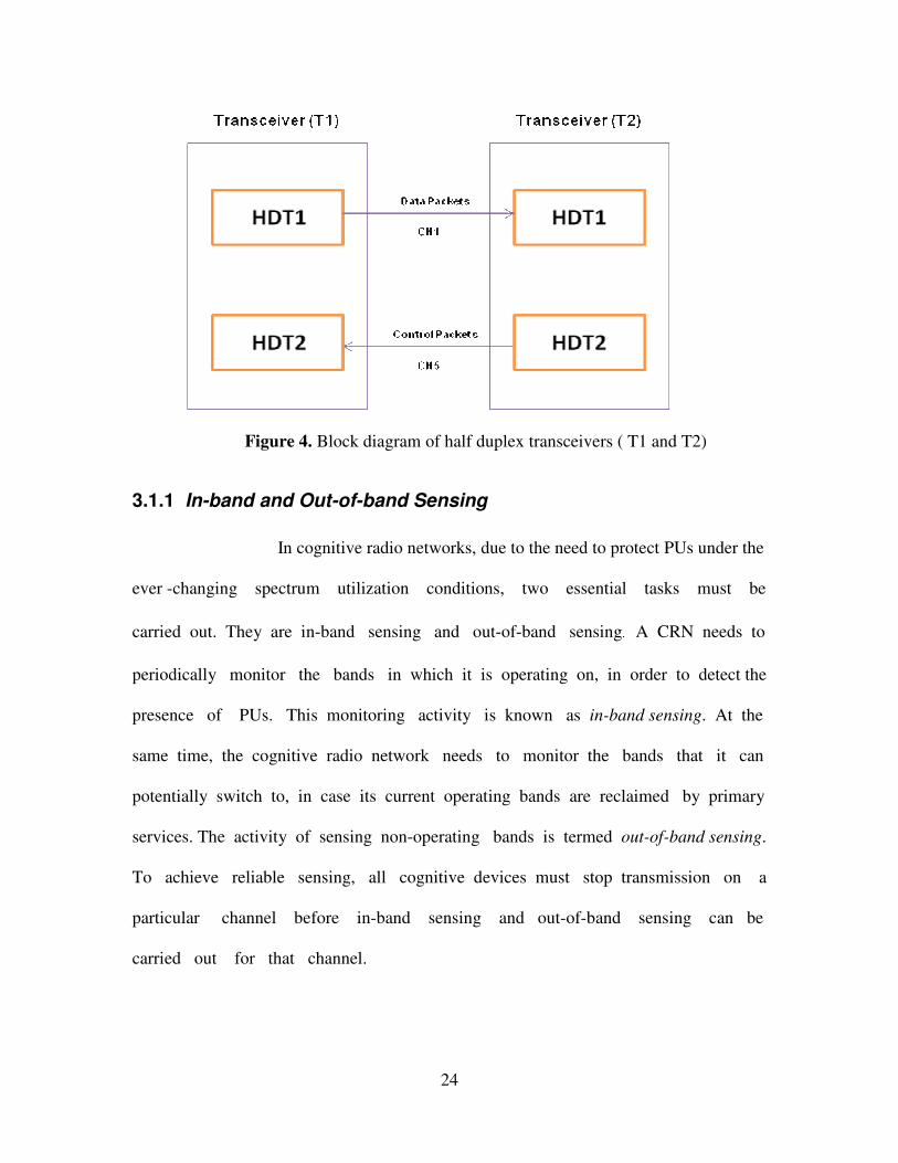
reduced delay of packets and less number of lost packets. Figure 4 illustrates the use of

half duplex transceivers. The figure shows that two transceivers T1 and T2 consist of

multiple half duplex transceivers HDT1 and HDT2. HDT1 and HDT2 use CH1 for

exchanging data packets and CH5 for exchanging control packets. The control packets

usually consists of the information about the channels based on the channel selection

criteria.

24

Figure 4. Block diagram of half duplex transceivers ( T1 and T2)

3.1.1 In-band and Out-of-band Sensing

In cognitive radio networks, due to the need to protect PUs under the

ever -changing spectrum utilization conditions, two essential tasks must be

carried out. They are in-band sensing and out-of-band sensing. A CRN needs to

periodically monitor the bands in which it is operating on, in order to detect the

presence of PUs. This monitoring activity is known as in-band sensing. At the

same time, the cognitive radio network needs to monitor the bands that it can

potentially switch to, in case its current operating bands are reclaimed by primary

services. The activity of sensing non-operating bands is termed out-of-band sensing.

To achieve reliable sensing, all cognitive devices must stop transmission on a

particular channel before in-band sensing and out-of-band sensing can be

carried out for that channel.

25

3.2. Channel Selection

Channel selection can be done easily if each node is equipped with multiple half

duplex transceivers. One transceiver is used for carrying the data communication while

the other is used to look up for the other channels. Channel selection can be done using

the following factors.

1. Channel Utilization

2. Channel Goodput

2.1 Packet Error Rate (PER)

3. Channel Slot

All these factors are combined into a metric called Channel Score.

Channel Slot is also called as spectrum hole or predicted white space duration. It

usually consists of frequency bands assigned to PUs. But at geographic location and at

particular time some of these frequency bands are under utilized by the PUs [17]. These

bands together are called as white spaces and the time for which these bands last is

considered as the white space duration or channel slot or spectrum hole. Spectrum

utilization can be improved significantly by allowing the SUs to access the spectrum hole

which is left unattended by the PUs. Hence the concept of CR is introduced in case of

spectrum hole because they promote efficient usage of the spectrum by exploiting the

existence of the spectrum holes [17].

Channel Score is an important criterion to identify channels that

have better transmission. It takes into consideration all of the above factors used for

selecting the channels.

26

3.3. Channel Utilization

According to the Intelli MAC protocol, the channel utilization factor indicates the

percentage of the channel which is under usage by the PUs. This factor will help in

identifying the best possible transmitting channel in combination with PER. Based on

the channel utilization by the PUs and PER, the SUs can identify the best possible

channel that is available. All SUs consider the channel utilization factor before

transmitting on the particular channel. The channel utilization factor is given by

the following formula.

Channel Utilization = Percentage of channel under usage by the PUs

From the OC-MAC protocol, a linear prediction model is used to

update the channel utilization for a particular time slot ‘t’[1]. The channel utilization is

given by the following formula. Ut = αUt−1 + (1 − α) * ( )

Ut−1 is the exact utilization of the last time slot t-1 and is the average

experienced utilization in the past [1]. α is a constant value. It is determined in such

a way that Ut approximates the exact utilization of the last time slot Ut−1 as accurately as

possible. The value of α is between 0 and 1 [1].

3.4. Channel Goodput

Channel goodput is usually measured as the amount of digital data that has been

received successfully over unit time. There are many factors that affect goodput such as

traffic load, shared channel capacity among the users, packet loss due to congestion and

packet error.

27

Goodput, according to Intelli MAC protocol, is defined based on the number of

packets that are received successfully over unit time. The proposed protocol uses fixed

size packets only.

Goodput = Number of packets received successfully / Unit time

Packet Error Rate (PER)

The proposed protocol takes into consideration, the Packet Error Rate (PER). Packet

Error Rate is the fraction of transmitted packets not received successfully by the

receiver. Normally it varies from one channel to another. The amount of usable data

received on each channel will vary according to PER. The amount of data successfully

received over a channel is given by the following equation.

Packets Successfully Received = Packets Sent * (1 – PER)

Throughput in case of OC-MAC protocol [1] is calculated based on the packet

size, predicted white space duration and an aggressive parameter β. The main purpose of

aggressive parameter value in OC-MAC protocol is to determine the estimated white

space duration [1]. β reflects the confidence in estimating the white space duration. Its

value ranges between 0 and 1. According to [1] the CR behaves aggressively when the

parameter value is close to 1 and behaves passively when the value is close to 0.

Throughput on the channel varies as the aggressive parameter value β changes from 0 to

1. A larger β value indicates more white space duration to be used. As the value of β

approaches 1, then there are more chances of colliding with PUs. This is because the

larger β value indicates the maximum time that SUs can transmit which can result in

interference to the PUs transmission when they start accessing the particular channel.

Throughput in [1] is defined by the following formula.

28

Throughput(x) =β ×(slot(x) – LC/Packet_size(x))`

From the throughput obtained, goodput is measured using the following formula.

Goodput(x) = Throughput(x) * (1-PER)

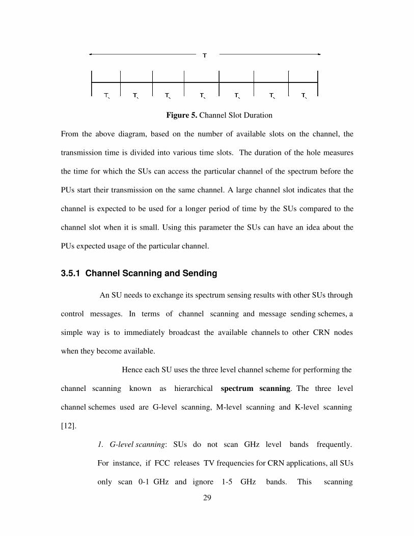
3.5. Channel Slot (Predicted white space duration)

There are two distinct classes of spectrum holes that a CRN needs to identify.

They are global holes and local holes [12]. Global holes are the unused frequency bands

which can be detected by the SUs in the entire network or large geographical area.

Local holes, on the other hand, are the unused frequency bands that can be identified by

the SUs in a small geographical area. These holes may not be identified by the users in

the other area. The CRN uses the holes that are identified in these bands for data

transmission [12].

According to the OC-MAC protocol, the channel slot is dependent on the channel

rate and the packet size [1]. Using the channel utilization and the channel threshold the

CR nodes can compute the maximum slot number for each channel. The maximum slot

number of channel is given by the following formula [1].

Slot (x) >= |log (Utilize(x))/log (Threshold(x))|

The channel slot is defined differently in the Intelli MAC layer protocol. This

protocol takes into consideration both the number of vacant slots available and also the

time duration of each slot. Let ‘T’ is the total time duration for data transmission on the

channel. ‘S’ be the number of vacant slots available on the channel. Every slot is

associated with the time period ‘Ts’.

29

Figure 5. Channel Slot Duration

From the above diagram, based on the number of available slots on the channel, the

transmission time is divided into various time slots. The duration of the hole measures

the time for which the SUs can access the particular channel of the spectrum before the

PUs start their transmission on the same channel. A large channel slot indicates that the

channel is expected to be used for a longer period of time by the SUs compared to the

channel slot when it is small. Using this parameter the SUs can have an idea about the

PUs expected usage of the particular channel.

3.5.1 Channel Scanning and Sending

An SU needs to exchange its spectrum sensing results with other SUs through

control messages. In terms of channel scanning and message sending schemes, a

simple way is to immediately broadcast the available channels to other CRN nodes

when they become available.

Hence each SU uses the three level channel scheme for performing the

channel scanning known as hierarchical spectrum scanning. The three level

channel schemes used are G-level scanning, M-level scanning and K-level scanning

[12].

1. G-level scanning: SUs do not scan GHz level bands frequently.

For instance, if FCC releases TV frequencies for CRN applications, all SUs

only scan 0-1 GHz and ignore 1-5 GHz bands. This scanning

30

typically occurs every 1 hour or even for longer time. This type of

scanning is useful for the SUs to identify PUs because some PUs work in

the GHz range channel.

2. M-level scanning: Within each GHz band there are about one hundred

10MHz - wide bands. The SUs can scan all these hundred bands to detect the

presence of PUs. The SUs in this scanning level uses a shorter period

than G-level scanning. Scanning time typically takes 10 minutes for each

band. As shown in Figure 6, between 1 and 2GHz, an SU could scan the

availability of different 10 MHz bands such as from 1.01 to 1.02 GHz.

3. K-level scanning: This level of scanning refers to the finest band

detections. There are about ten 100 KHz bands that are present within each

MHz band. Typically, each 100 KHz could serve as a communication band.

Scanning time for these bands usually takes lesser time than M-level scanning.

As shown in Figure 6, within the 10 MHz band, an SU could scan the

availability of different 100 K bands.

Figure 6. Channel scanning scheme

31

3.6. Channel Score

According to OC-MAC protocol [1], channel score is the minimal

throughput among transmitter and receiver. Channel score is given by the

following formula [1].

Channel Score = Minx{Throughputtran(x), Throughputrecv(x)}

The receiver chooses the channel with largest score and informs the

transmitter of the choice [1].

According to the OC-MAC protocol when a receiver B receives

a RTS (Request To Send) packet from sender A, then the channel state table will

be updated. The sender sends its available channel set and possible transmission

durations in RTS packet to the receiver [1]. Within the channel state table, available

timer on the channel and the channel utilization are used to record the status of the

channels [1]. The receiver B will find the overlapping channel set between A’s and

B’s available lists and uses the evaluating function to allot a score to the

channels [1]. The most appropriate channel is identified based on the following

formula that indicates which CR pairs can send most packets cumulatively [1].

Max(Minx{Throughputtran(x), Throughputrecv(x)})

According to the OC-MAC protocol if there are more than one channel that have

the same packet number then the channel with maximum transmission rate will

be selected. A random choice is used when there are channels with same packet

number and transmit rate. After deciding on the channel, the receiver B sends a

CTS (Clear To Send) packet to A with the channel index and maximum packet

number included in it. If B cannot find a suitable channel or the maximum number of

32

packets that were to be transmitted is zero, B will do nothing and A’s timer to

receive the CTS will expire [1].

According to Intelli MAC protocol, channel score is used for selecting the best

channel based on channel goodput and predicted white space duration. The channel

selection is being done using the channel score. If a particular channel has higher

channel score, it means that it can send more data. It also indicates that the goodput

on the channel is more. Channel score is computed as follows.

Channel Score = S * Θ

Where ‘Θ’ is the effective goodput on the channel and ‘S’ gives the expected number of

consecutive vacant slots available on the channel. S is used to measure the

expected white space duration available for a particular channel on which the SUs can

transmit. The effective goodput measured in bits per second can be measured using the

following formula.

Θ = w*(1-q)

Where ‘w’ is the throughput and ‘q’ is the bit error rate. The number of consecutive slots

‘S’ is measured using the following formula.

1 - (1-u)S = p

1-p = (1-u)S

After applying logarithm on both sides, the above equation will be as follows.

log (1-p) = S * log (1-u)

S = |log (1-p) / log (1-u)|

Where ‘u’ is the probability that a time slot will be used by any PUs. The probability ‘u’

is estimated from the expected channel utilization. The number of consecutive slots has to

33

be found out so that the probability that none of the time slot will be used by the PU is

‘p’. ‘1-u’ is the probability of one slot not being used and ‘(1-u)S’

is the probability of ‘S’

slots not being used. ‘1 - (1-u)S < p

’ is the probability at least one of the ‘S’ slots being

used.

3.7. Channel State Table

The channel state table contains information about different channels. It is

located in every SUs memory. It is used to select the best channel for

communication. It contains the information about channel number, channel score,

channel slot and channel utilization. Before transmitting data on channel both the SUs

(transmitter and receiver) will access their own channel state table for obtaining

information about the channel. Since each node is associated with the channel state

table, it is easier to identify and assess the channel status before transmission.

According to the proposed protocol, the SUs can make a selection about channel

based on the PUs transmission.

This paragraph explains the selection of best channel among the available

channels for data transmission between two SUs using their own channel state tables.

Since the channel state tables contain the information about channel number, channel

score, channel slot and channel utilization, it is easier and a quicker process to select

among the group of similar channels or group of different channels. Consider that

there are three channels with channel state table available for both the SUs A and B to

access. Table 1 shows the different channels available with respect to the users A and

B and respective channel utilization and channel score values.

34

Table 1: Three different channels with channel utilization and channel score values

From the channel state tables of the two SUs, two channels CH1 and CH3 are

common for both A and B. For selecting the best channel among A and B, the channel

state table is used to check for the available channel score and channel utilization of

two channels. The average channel score and channel utilization of both the common

channels are taken into account.

The average channel score calculated for the channels CH1 and CH3 is shown below.

CH1 = (0.45+0.193)/2 = 0.33

CH3 = (0.135+0.4)/2 = 0.27

The average channel utilization for the channels CH1 and CH3 is measured as

follows.

CH1 = (0.60+0.60)/2 = 0.60

CH3 = (0.80+0.07)/2 = 0.48.

From the above averages, it is shown that CH1 has higher channel score compared to

CH3 and also the channel utilization of CH1 is higher compared to CH3.Hence CH1

is considered to be the best available channel for communication among the SUs.

In case if the channel score for CH1 is higher and channel utilization for CH3 is higher

then the users randomly select one among the two channels.

35

3.8. Harmonious Channel (HC)

A Rendezvous Channel (RC) is used to manage the entire network [3]. Some of

the tasks of the RC are inter channel synchronization, neighborhood discovery and load

balancing.

According to the C-MAC protocol [3], one channel is selected at random as RC.

The Harmonious Channel (HC) concept is proposed in the Intelli MAC protocol. The

Intelli MAC layer protocol follows certain selection procedure for selecting the HC. Like

RC, the HC is also used to manage the network by synchronization and discovery.

The HC is mainly used in carrying the coordination among different SUs

The coordination among different SUs takes place by exchanging control packets. It

is important to select the particular channel that will act as a HC. As discussed in

section 3.7, each SU keeps a channel state table in its memory. The HC can be used

to carry out the transmission among the SUs in case of PUs presence on a

particular channel. This means that if the SUs transmission on a particular channel is

being interrupted by the PUs, then the HC can be used by the SUs to shift

quickly and continue with their transmission. The selection of the HC follows certain

procedure. It makes use of the channel state table, channel utilization factor and channel

score. Each SU is associated with a HC field. During the time of PUs transmission

over a particular channel, SUs will perform the spectrum sensing in order to

determine the HC for their transmission. When any one SU identifies a HC then it

will update its own HC field first and then sends the information about the newly

discovered HC to rest of the SUs. All remaining SUs will also update their

corresponding HC fields. If HC field cannot be updated based on the PUs transmission

36

then the SUs will determine the HC based on the channel utilization and channel

score. If there are two channels that can be used as HC having the same channel

utilization and channel score then a random selection procedure is followed. The

SUs will choose one among the two channels as HC by randomly selecting one.

The same selection procedure is followed if there are more than two HCs. One

main advantage in selecting HC is that it is able to count the number of PUs transmission

on the particular channel.

3.8.1 HC Switching

Each HC will be equipped with a timer at each node. After identifying a particular

channel as HC, then a timer will be set within the HC at each node. The timer will start

only at the time of data transmission among users. In this way all the users will be in

synchronization with HC. When the timer of one HC expires, even if transmission among

the users does not end, all users that were involved in the transmission will move to

another HC and continue with the transmission. The users which are not transmitting in

HC do not have to shift to a new HC. In order to keep track of the timers in current HC

and to shift to new HC when timer expires, all users should have the capability of having

multiple half duplex transceivers. By using this feature one transceiver can takes care of

the timer on primary HC and the other is used for switching to secondary HC.

37

3.8.2 HC Selection

Timers are used in case of all HCs to choose a better one. The timer will be set

and reset based on the data that is going to be transmitted. The timer will start counting

when a user starts transmitting. At the end of all transmissions the timer will be updated.

Now when PUs come to access a particular channel, all SUs will move to the HC for

transmission. The time at which the PUs have arrived will be noted. According to Intelli

MAC layer protocol, Channel Transmission Time (CTT) is the time between the SUs

first transmission and the PUs presence on the channel.

3.8.3 PU Notification

If an SU has detected the presence of PU on a particular channel, it will

update its channel state table first and then notifies the rest of the SUs about PUs

presence. Now, rest of the SUs that listen to this information on the channel will update

their respective channel state table. Further the SUs can also obtain the information

about which channel to switch to (i.e., which channel is free of PUs). Since the

channel state table contains the channel utilization criterion, hence network resources

can be saved because there is no need for the other SUs to sense for the PUs and

also for the vacant channels.

3.8.4 PU Detection Recovery

When a SU determines the existence of PUs, then it has to switch to another

channel. This can be made possible with the help of multiple half duplex transceivers.

While one transceiver can check for the incoming PUs, the other transceiver checks

38

for other potential channels. SUs after detecting PUs presence and the channel to

which they have to shift, the channel state table will be updated. All the SUs have

to check their channel state table to obtain the information about the channel

before transmission. Hence those SUs present on the channel can also get the

information about the PUs and the vacant channel. Also using the channel state

table all SUs on a particular channel can learn about the occupancy of the

spectrum in their vicinity.

3.9. Performance Evaluation

This section shows the simulation results of the proposed (Intelli MAC Layer)

protocol and OC-MAC protocol. The comparison of both protocols is shown from the

views of Channel Goodput, Channel Utilization, Channel Slot and Channel Score. All

simulations were performed using NS-2 version 2.32 (Network Simulator). The protocol

test scenario is shown below.

Primary Network - 802.11b WLAN

No of users - 4 PUs and 8 SUs

No of Channels - 6

Data Rates - 2Mbps, 5Mbps, 7Mbps and 11Mbps

PER - 0.02, 0.04, 0.06, 0.08

39

The primary network used was 802.11b WLAN because of good signal range and

interference can be easily avoided. To differentiate one channel from the other, each

channel is set with data rate and PER separately. The following table shows different data

rates and PER for six different channels.

Table 2: Data rates and PER for 6 channels

3.9.1 Channel Utilization

The following figure shows channel utilization factor that SUs take into consideration in

case of Intelli MAC layer protocol. It shows that the channel utilization for CH-2 is

higher compared with the other channels and channel utilization for CH-3 is the

lowest utilization among all the channels. This is because CH-2 is having a

data rate of 2Mbps and PER of 0.02 and CH-3 is having a data rate of 7Mbps

but with PER of 0.08. Also, channel utilization is dependent on the channel

throughput, data rate and PER and more importantly how much data to be

transmitted and how the PUs schdule data transmission.

40

Figure 7. Channel Utilization in case of Intelli MAC Protocol

The following figure shows the channel utilization in case of OC-MAC

protocol. The channel utilization in case of CH-2 and CH-4 is more compared to the

other channels. This is due to the collision rate among the packet is less, that is the

tolerable damage threshold is 0.01.

Figure 8. Channel Utilization in case of OC-MAC protocol

41

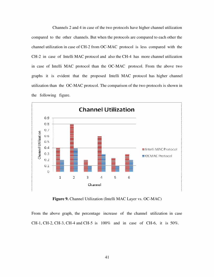
Channels 2 and 4 in case of the two protocols have higher channel utilization

compared to the other channels. But when the protocols are compared to each other the

channel utilization in case of CH-2 from OC-MAC protocol is less compared with the

CH-2 in case of Intelli MAC protocol and also the CH-4 has more channel utilization

in case of Intelli MAC protocol than the OC-MAC protocol. From the above two

graphs it is evident that the proposed Intelli MAC protocol has higher channel

utilization than the OC-MAC protocol. The comparison of the two protocols is shown in

the following figure.

Figure 9. Channel Utilization (Intelli MAC Layer vs. OC-MAC)

From the above graph, the percentage increase of the channel utilization in case

CH-1, CH-2, CH-3, CH-4 and CH-5 is 100% and in case of CH-6, it is 50%.

42

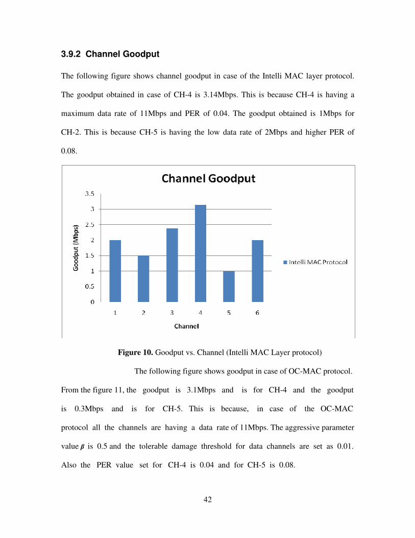
3.9.2 Channel Goodput

The following figure shows channel goodput in case of the Intelli MAC layer protocol.

The goodput obtained in case of CH-4 is 3.14Mbps. This is because CH-4 is having a

maximum data rate of 11Mbps and PER of 0.04. The goodput obtained is 1Mbps for

CH-2. This is because CH-5 is having the low data rate of 2Mbps and higher PER of

0.08.

Figure 10. Goodput vs. Channel (Intelli MAC Layer protocol)

The following figure shows goodput in case of OC-MAC protocol.

From the figure 11, the goodput is 3.1Mbps and is for CH-4 and the goodput

is 0.3Mbps and is for CH-5. This is because, in case of the OC-MAC

protocol all the channels are having a data rate of 11Mbps. The aggressive parameter

value β is 0.5 and the tolerable damage threshold for data channels are set as 0.01.

Also the PER value set for CH-4 is 0.04 and for CH-5 is 0.08.

43

Figure 11. Goodput vs. Channel (OC-MAC protocol)

The following figure shows the comparison between Intelli MAC layer protocol

and OC-MAC protocol.

Figure 12. Channel Goodput (Intelli MAC Layer vs. OC-MAC)

44

3.9.3 Channel Slot

The following graph shows spectrum hole duration for six different channels in

case of Intelli MAC Layer protocol. The spectrum hole duration on a channel in case

of Intelli MAC layer protocol is measured from the product of the number of consecutive

slots and the duration of each time slot. The number of consecutive slots is dependent on

the channel utilization factor. From the following figure, the spectrum hole duration on

CH-3 and CH-5 is higher compared to the other channels. This is due to the reason that

the channel utilization of both the channels is less. That means the PUs that are accessing

these particular channels are less. Hence, these two channels have larger spectrum hole

duration.

Figure 13. Channel slot in case of Intelli MAC Protocol

The following figure shows the number of consecutive slots that are available on each

channel and the spectrum hole duration on the channel in case of OC-MAC protocol.

Channel slot in case of OC-MAC protocol is dependent on the channel utilization and the

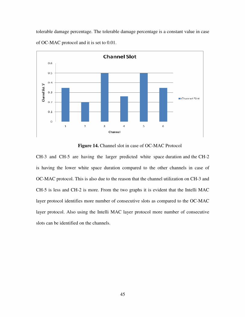
45

tolerable damage percentage. The tolerable damage percentage is a constant value in case

of OC-MAC protocol and it is set to 0.01.

Figure 14. Channel slot in case of OC-MAC Protocol

CH-3 and CH-5 are having the larger predicted white space duration and the CH-2

is having the lower white space duration compared to the other channels in case of

OC-MAC protocol. This is also due to the reason that the channel utilization on CH-3 and

CH-5 is less and CH-2 is more. From the two graphs it is evident that the Intelli MAC

layer protocol identifies more number of consecutive slots as compared to the OC-MAC

layer protocol. Also using the Intelli MAC layer protocol more number of consecutive

slots can be identified on the channels.

46

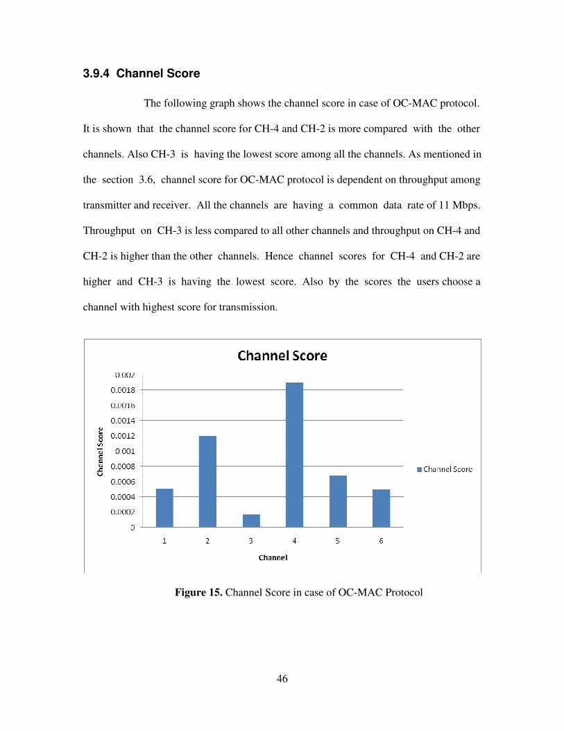
3.9.4 Channel Score

The following graph shows the channel score in case of OC-MAC protocol.

It is shown that the channel score for CH-4 and CH-2 is more compared with the other

channels. Also CH-3 is having the lowest score among all the channels. As mentioned in

the section 3.6, channel score for OC-MAC protocol is dependent on throughput among

transmitter and receiver. All the channels are having a common data rate of 11 Mbps.

Throughput on CH-3 is less compared to all other channels and throughput on CH-4 and

CH-2 is higher than the other channels. Hence channel scores for CH-4 and CH-2 are

higher and CH-3 is having the lowest score. Also by the scores the users choose a

channel with highest score for transmission.

Figure 15. Channel Score in case of OC-MAC Protocol

47

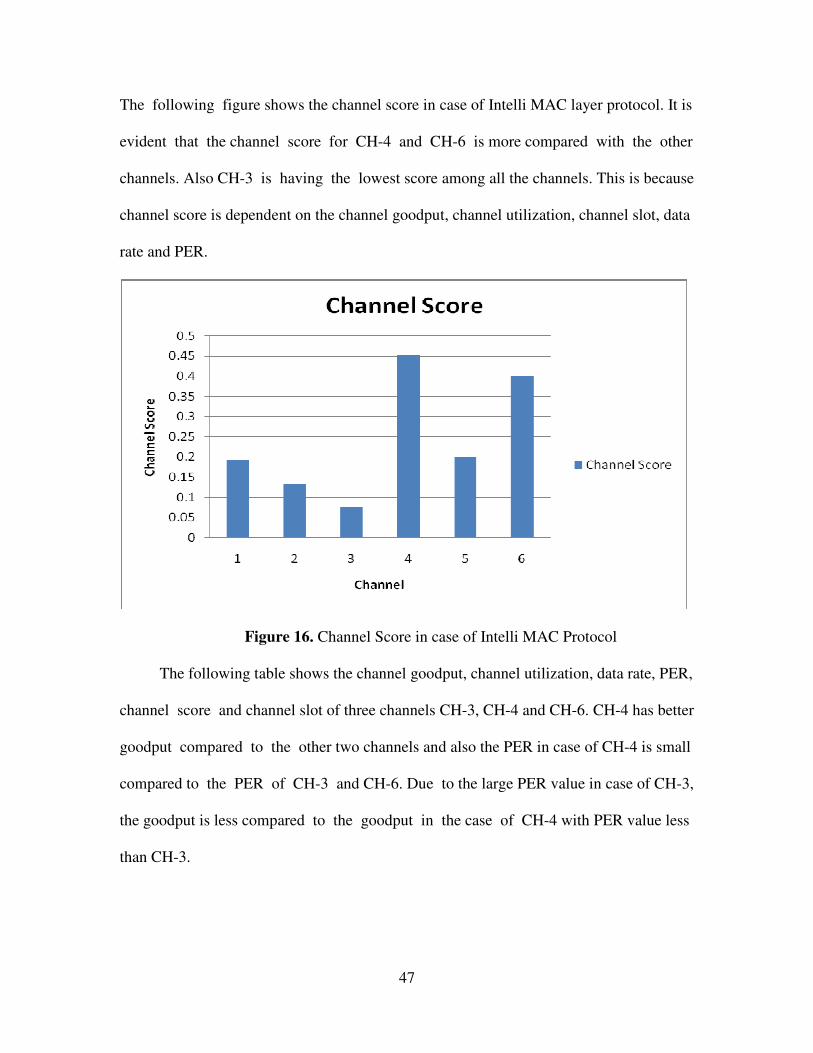
The following figure shows the channel score in case of Intelli MAC layer protocol. It is

evident that the channel score for CH-4 and CH-6 is more compared with the other

channels. Also CH-3 is having the lowest score among all the channels. This is because

channel score is dependent on the channel goodput, channel utilization, channel slot, data

rate and PER.

Figure 16. Channel Score in case of Intelli MAC Protocol

The following table shows the channel goodput, channel utilization, data rate, PER,

channel score and channel slot of three channels CH-3, CH-4 and CH-6. CH-4 has better

goodput compared to the other two channels and also the PER in case of CH-4 is small

compared to the PER of CH-3 and CH-6. Due to the large PER value in case of CH-3,

the goodput is less compared to the goodput in the case of CH-4 with PER value less

than CH-3.

48

Table 3: Three channels with channel goodput, channel utilization, data rate, PER,

channel score and channel slot values. From the above table, data rate for CH-3 is more than CH-6 and also the channel goodput

and PER are more for CH-3 than CH-6. But in case of channel slot, CH-3 is having more

number of vacant slots compared to CH-6. Since there is no major difference in terms of

channel goodput, channel utilization and channel slot between CH-3 and CH-6, CH-6

will be considered to be better for transmission than CH-3 because of the low PER value.

From the figures 15 and 16 it is evident that the CH-4 is having the highest score

compared with the other channels and CH-3 is having the lowest score among all the

channels. But in case of the Figure 15 (OC-MAC protocol), CH-2 has the second highest

channel score, this is because CH-2 has the higher data rate of 11 Mbps and has higher

channel utilization of 0.4 and goodput of 1.3 Mbps when compared to all other channels.

From the Figure 16 (Intelli MAC layer protocol), CH-6 has the second highest channel

score, this is because CH-6 has a data rate of 5 Mbps and the goodput on the channel is

2 Mbps and has a channel utilization of 0.3.

49

Chapter 4 NS-2 (Network Simulator)

NS-2 is a discrete event simulator mainly used for networking research.

NS-2 offers wide support for simulation of TCP, routing and multicast protocols over

wired and wireless networks [13]. NS-2 is written in C++ and an Object oriented version

of Tcl called OTcl. Tcl is a scripting language widely used for writing scripting

applications, GUIs and testing. There are some interesting features about Tcl [14].

1. Tcl is platform independent. Hence it can be used on Win32, Unix or Linux based

machines.

2. It has simple syntax rules.

3. Everything can be dynamically redefined and overridden.

4. Everything is command based including the structure of the language.

5. Readily extensible via C, C++, Java, etc.,

6. Due to compactness of Tcl scripts, it is easier to maintain the codes.

4.1. C++/Tcl

The software programming library interface allows the integration of C++ into

Tcl and vice versa. Some of the features of this library are.

1. Supporting the extension of Tcl with C++ modules and embedding Tcl

in C++ applications.

2. C++ functions can be used as commands in Tcl.

3. Classes and class member functions can be defined easily.

4. Easy to manipulate Tcl lists and objects from the C++ code.

50

For installing NS-2 we need to make sure that the following components are available.

1) tcl-8.3.2

2) tk-8.3.2

3) otcl-1.0a7

4) tclcl-1.0b11

5) ns-2.3b2a

6) nam-1.0a10

7) mglinstaller (for Windows), or xgraph-12.1 (for Unix)

4.2. NS-2 Installation Instructions

The major advantage of NS-2 is that it can be Windows as well as on Unix/Linux

based machines.

4.2.1 NS-2 installation on UNIX/LINUX Machine

NS-2 has been basically designed to run on most of the UNIX based OS.

Using VMWare Player a Linux like environment can be created on normal Windows

machine and using Cygwin a Unix based environment can be created on normal

Windows machine. The initial step in installing NS-2 is to download a copy of

ns-allinone-x.xx version from the following website http://sourceforge.net/project/.

The version that has been used for this thesis is ns-allinone-2.32. Then, from the

command prompt the following lines of code are executed to unzip the folder.

tar -xzf ns-allinone-2.32.tar.gz

cd ns-allinone-2.29

./install

After the installation of ns-2.32 is over the following text is shown in the command

window.

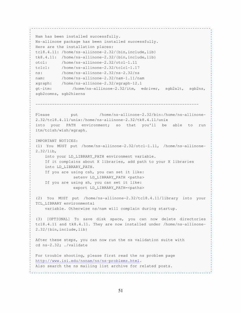
51

Nam has been installed successfully.

Ns-allinone package has been installed successfully.

Here are the installation places:

tcl8.4.11: /home/ns-allinone-2.32/{bin,include,lib}

tk8.4.11: /home/ns-allinone-2.32/{bin,include,lib}

otcl: /home/ns-allinone-2.32/otcl-1.11

tclcl: /home/ns-allinone-2.32/tclcl-1.17

ns: /home/ns-allinone-2.32/ns-2.32/ns

nam: /home/ns-allinone-2.32/nam-1.11/nam

xgraph: /home/ns-allinone-2.32/xgraph-12.1

gt-itm: /home/ns-allinone-2.32/itm, edriver, sgb2alt, sgb2ns,

sgb2comns, sgb2hierns

---------------------------------------------------------------------

Please put /home/ns-allinone-2.32/bin:/home/ns-allinone-

2.32/tcl8.4.11/unix:/home/ns-allinone-2.32/tk8.4.11/unix

into your PATH environment; so that you'll be able to run

itm/tclsh/wish/xgraph.

IMPORTANT NOTICES:

(1) You MUST put /home/ns-allinone-2.32/otcl-1.11, /home/ns-allinone-

2.32/lib,

into your LD_LIBRARY_PATH environment variable.

If it complains about X libraries, add path to your X libraries

into LD_LIBRARY_PATH.

If you are using csh, you can set it like:

setenv LD_LIBRARY_PATH <paths>

If you are using sh, you can set it like:

export LD_LIBRARY_PATH=<paths>

(2) You MUST put /home/ns-allinone-2.32/tcl8.4.11/library into your

TCL_LIBRARY environmental

variable. Otherwise ns/nam will complain during startup.

(3) [OPTIONAL] To save disk space, you can now delete directories

tcl8.4.11 and tk8.4.11. They are now installed under /home/ns-allinone-

2.32/{bin,include,lib}

After these steps, you can now run the ns validation suite with

cd ns-2.32; ./validate

For trouble shooting, please first read the ns problem page

http://www.isi.edu/nsnam/ns/ns-problems.html.

Also search the ns mailing list archive for related posts.

52

Follow the instructions that are shown in the command window. These instructions

are very important for updating the environment variables. If we do not follow these

instructions then certain applications of NS-2 will encounter problems while

performing the simulations.

One more important thing to remember is to add ns-allinone-2.32/bin to the

path. Because this has the links to all of the executables that are created by NS-2.

After adding the environment variables the following commands are given at the

command prompt to test the installation.

cd ns-2.32

./validate

After the validation part is done, it indicates that the NS-2.32 has been installed

successfully and can be used for simulations purpose.

4.2.2 NS-2 installation on Windows Machine

The initial setup for the NS-2 is slightly different because NS-2 mainly runs on

Unix based machines. Hence in order to install NS-2 on Windows machine, Cygwin is

used. Cygwin is a Unix like environment and command line interface for Windows.

The major difference between installing the NS-2 on Windows machine and

on Unix/Linux Machine is the Cygwin installation. Windows require Cygwin,

because a Dynamic-link library (DLL) (cygwin1.dll) which acts as a Linux API

emulation layer providing Linux Application Programming Interface (API) functionality.

The installation instructions of Cygwin can be found in the following website

http://www.cygwin.com. Once the set up of Cygwin application is completed under

53

windows then the same installation instructions that were followed in case of Unix/Linux

based machines can be followed for Windows based machines.

54

Chapter 5 Conclusions and Future Work

Intelli MAC Layer protocol uses multiple half duplex transceivers to

perform in-band and out-of-band sensing in order to detect the channel for continuing

communication among the SUs and also to detect the presence of PUs. The Intelli

MAC Layer protocol emphasizes on the channel selection mainly. The channel

selection is based on properties like channel goodput, channel utilization,

channel score, channel slot and channel state table. With these properties a

better channel required for transmitting and receiving the data can be selected.

Intelli MAC protocol helps to reduce channel sensing time for the SUs.

Intelli MAC Layer protocol uses the concept of Harmonious Channel (HC).

The HC is mainly used in carrying the coordination among different SUs within the

same channel or among different channel or within the same spectrum. It is also used

to manage the network by synchronization and discovery.

5.1. Future Work

Full duplex transceivers are always advantageous compared with half duplex

transceivers. A single full duplex transceiver can perform the same amount of work done

by multiple half duplex transceivers. Also using the multiple half duplex transceivers,

they can increase the hardware capacity of the transmitter and receiver. Using Full duplex

transceivers in case of Intelli MAC protocol can result in selecting the best channel for

carrying the SUs data transmission in case of PUs presence. Also they can be able to

reduce the channel sensing time more when compared to the single half duplex

transceivers. On the other hand, the major disadvantages of using full duplex transceivers

55

are that they require complex hardware systems for installing on both transmitter and

receiver and more power.

Similar to the existing MAC layer protocols, the Intelli MAC Layer protocol does

not take into consideration the simultaneous transmission among PUs and SUs on the

channel. The SUs can be benefitted from simultaneous transmission. If the SUs are at the

end of transmission when the PUs start to transmit among themselves, then using the

simultaneous transmission method the SUs do not have to stop their transmission and

perform the spectrum scanning in order to look for HC. Instead of that, they can continue

and finish the transmission.

56

Chapter 6 Bibliography

[1] Shao-Yi Hung, Eric Hsiao-Kuang Wu and Gen-Huey Chen “An Opportunistic

Cognitive MAC Protocol for Coexistence with WLAN,” ICC 2008, pages 4059-4063.

[2] J. Mitola III, “Cognitive Radio: An integrated agent architecture for software defined

radio,” May 2000. Available at: http://citeseer.ist.psu.edu/568482.html.

[3] Carlos Cordeiro and Kiran Challapali “C-MAC: A Cognitive MAC Protocol for Multi

Channel Wireless Networks,” New Frontiers in Dynamic Spectrum Access Networks,

2007, DySPAN 2007, 2nd

IEEE International Symposium, 17-20 April 2007,

pp. 147-157.

[4] Rahul Patibandla, Fei Hu, Yang Xiao, “Cognitive Radio Adaptive Medium Access

Control (MAC) Design,” Chapter 8 in the book Cognitive Radio Networks by the CRC

Press, in Feb. 2008 - Vol. 1, Ch. 8, pp. 237 - 254.

[5] L. Ma, X. Han, and C.C. Shen, “Dynamic open spectrum sharing MAC protocol for

wireless ad hoc networks,” Proc. of DySPAN 2005, 1st IEEE International Symposium,

8-11 Nov 2005, pp. 201-213.

[6] D. Raychaudhuri and X. Jing, “A spectrum etiquette protocol for efficient

coordination of radio devices in unlicensed bands,” In Proceedings of the 14th

International Symposium on Personal, Indoor and Mobile Radio Communication, IEEE

2003, 7-10 Sept 2003, Vol. 1, pp. 172-176.

[7] P. Pawelczak, R. V. Prasad, L. Xia, and I. M Niemegeers, “Cognitive radio

emergency networks – requirements and design,” Proc. of DySPAN 2005, 8-11 Nov.

2005, pp. 601-606.

[8] P. Bahl, R. Chandra, and J. Dunagan, “SSCH: slotted seeded channel hopping for

capacity improvement in IEEE 802.11 ad-hoc wireless networks,” Proc. of MobiCom’04,

pp. 216-230.

[9] I. F. Akyildiz, W.Y. Lee, M. C. Vuran, and S. Mohanty, “NeXt generation/dynamic

spectrum access/cognitive radio wireless network: A survey,” Elsevier Computer

Networks, January 2006, pp. 1 - 30.

[10] A. Jayasuriya, S. Perreau, A. Dadej, and S. Gordon, “Hidden vs. exposed terminal

problem in ad hoc networks,” Proceedings of the Australian Telecommunications,

Networks and Architecture Conference (ATNAC 2004), Sydney 2004.

[11] FCC, ET Docket No 03-222 “Notice of Proposed rule making and order,” December

2003.

57

[12] Rahul Patibandla, Fei Hu, Yang Xiao, “Spectrum sensing in cognitive radio sensor

networks: towards ultra low overhead, distributed channel findings,” Int. J. Sensor

Networks, Vol. 3, No. 2, 2008.

[13] Greis Marc, “Tutorial for the Network Simulator ns”.

[14] Chung Jay and Claypool Mark, “NS By Example,” Worcester Polytechnic Institute.

[15] P802.11, IEEE Standard for Wireless LAN Medium Access Control (MAC) and

Physical Layer (PHY) Specifications, November 1997.

[16] Pradeep Kyasanur and Nitin H. Vaidya, “Routing and interface assignment in multi

channel multi interface wireless networks” In IEEE Communication Society/WCNC

2005, 13-17 March 2005, Vol. 4, pp. 2051-2056.

[17] Simon Haykin, “Cognitive Radio: Brain-Empowered Wireless Communications” in

IEEE Journal on selected areas in communications, February 2005, Vol. 23, No. 2,

pp. 201-220.

[18] eMarketer (2002) Available at: http://www.emarketer.com/.

[19] Fei Hu, Yang Xiao, “Cognitive Radio Adaptive Medium Access Control (MAC)

Design” in the book Cognitive Radio Networks by the CRC Press, Vol. 1, Ch. 1,

pp. 22 – 55, February 2008.

[20] 3Com, “IEEE 802.11b Wireless LANs”, technical paper. Available at

http://www.3com.com/other/pdfs/infra/corpinfo/en_US/50307201.pdf, pp. 1-12, January

2000.

[21] H. Koubaa, “ Fairness - enhanced multiple control channels MAC for ad hoc

networks,” Proc. of IEEE VTC – spring 2005, 30 May – 1 June 2005 Vol. 3,

pp. 1504-1508 .

[22] A. Boukerche, T. Huang, and K. Abrougui, “Design and performance evaluation of a

QoS- based dynamic channel allocation protocol for wireless and mobile networks,” In

proceedings of 13th

IEEE international symposium on Modeling, analysis, and

simulation of computer and telecommunication systems (MASCOTS’05), 2005,

pp. 445-452.

[23] D. Cabric, S. M. Mishra, and R. W. Brodersen, “Implementation issues in spectrum

sensing for cognitive radios,” in Signals, Systems and Computers, Vol. 1, 2004,

pp. 772–776.

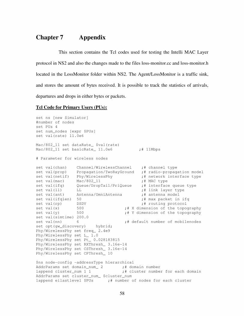
58

Chapter 7 Appendix

This section contains the Tcl codes used for testing the Intelli MAC Layer

protocol in NS2 and also the changes made to the files loss-monitor.cc and loss-monitor.h

located in the LossMonitor folder within NS2. The Agent/LossMonitor is a traffic sink,

and stores the amount of bytes received. It is possible to track the statistics of arrivals,

departures and drops in either bytes or packets.

Tcl Code for Primary Users (PUs):

set ns [new Simulator]

#number of nodes

set PUs 4

set num_nodes [expr $PUs]

set val(rate) 11.0e6

Mac/802_11 set dataRate_ $val(rate)

Mac/802_11 set basicRate_ 11.0e6 ;# 11Mbps

# Parameter for wireless nodes

set val(chan) Channel/WirelessChannel ;# channel type

set val(prop) Propagation/TwoRayGround ;# radio-propagation model

set val(netif) Phy/WirelessPhy ;# network interface type

set val(mac) Mac/802_11 ;# MAC type

set val(ifq) Queue/DropTail/PriQueue ;# interface queue type

set val(ll) LL ;# link layer type

set val(ant) Antenna/OmniAntenna ;# antenna model

set val(ifqlen) 50 ;# max packet in ifq

set val(rp) DSDV ;# routing protocol

set val(x) 500 ;# X dimension of the topography

set val(y) 500 ;# Y dimension of the topography

set val(simtime) 200.0

set val(nn) 6 ;# default number of mobilenodes

set opt(gw_discovery) hybrid;

Phy/WirelessPhy set freq_ 2.4e9

Phy/WirelessPhy set L_ 1.0

Phy/WirelessPhy set Pt_ 0.028183815

Phy/WirelessPhy set RXThresh_ 3.16e-14

Phy/WirelessPhy set CSThresh_ 3.16e-14

Phy/WirelessPhy set CPThresh_ 10

$ns node-config -addressType hierarchical

AddrParams set domain_num_ 2 ;# domain number

lappend cluster_num 1 1 ;# cluster number for each domain

AddrParams set cluster_num_ $cluster_num

lappend eilastlevel $PUs ;# number of nodes for each cluster

59

#create trace objects for ns and nam

set tracefd [open rd20095.tr w]

$ns use-newtrace

$ns trace-all $tracefd

$ns eventtrace-all

set namfile [open rd20095.nam w]

$ns namtrace-all-wireless $namfile $val(x) $val(y)

set chan [new $val(chan)]

set topo [new Topography]

$topo load_flatgrid $val(x) $val(y)

#Choose method for gateway discovery

if {$opt(gw_discovery) == "proactive"} {

Agent/AODV set gw_discovery 0

}

if {$opt(gw_discovery) == "hybrid"} {


}

if {$opt(gw_discovery) == "reactive"} {


}


# Create God

create-god [expr $PUs]

set chan_1 [new $val(chan)]






# creating base station

$ns node-config -adhocRouting $val(rp) \

-llType $val(ll) \

-macType $val(mac) \

-ifqType $val(ifq) \

-ifqLen $val(ifqlen) \

-antType $val(ant) \

-propType $val(prop) \

-phyType $val(netif) \

-channel $chan_6 \

-topoInstance $topo \

-wiredRouting OFF \

-agentTrace OFF \

-routerTrace OFF \

-macTrace OFF \

-movementTrace OFF \

# creating mobile nodes

for {set i 0} {$i < $PUs} {incr i} {

set gw($i) [$ns node 1.0.[expr $i + 1]]

60

$gw($i) random-motion 0 ;# disable random motion

puts "PU $i has been created ..."

}

for {set i 0} {$i < $PUs} {incr i} {

set udp_($i) [new Agent/UDP]

$ns attach-agent $gw($i) $udp_($i)

set null_($i) [new Agent/LossMonitor]

$ns attach-agent $gw($i) $null_($i)

}

for {set i 0} {$i < $PUs } {incr i} {

if {$i == ($PUs-1)} {

$ns connect $udp_($i) $null_(0)

} else {

set j [expr $i+1]

$ns connect $udp_($i) $null_($j)

}

set cbr_($i) [new Application/Traffic/CBR]

$cbr_($i) attach-agent $udp_($i)

$cbr_($i) set type_ CBR

$cbr_($i) set packet_size_ 1000

$cbr_($i) set rate_ 11Mb

$cbr_($i) set random_ false

#$ns at 0.0 "$cbr($i) start"

#$ns at $val(simtime) "$cbr($i) stop"

#$ns at 0.0 "$cbr([expr $i +1]) start"

#$ns at $val(simtime) "$cbr([expr $i +1]) stop"

}

for {set i 0} {$i < $val(simtime)} {incr i 1} {

for {set j 0} {$j < $PUs} {incr j} {

set rng [new RNG]

$rng seed 0

set rand1 [new RandomVariable/Uniform]

$rand1 use-rng $rng

$rand1 set min_ 0.0

$rand1 set max_ 1.0

set x [expr [$rand1 value]]

set y [expr [$rand1 value]]

$gw($j) set X_ $x

$gw($j) set Y_ $y

}

#puts "Random Number at $i second:$x"

}

for {set i 0} {$i < $PUs } {incr i} {

61

$ns at 1.0 "$cbr_($i) start"

$ns at $val(simtime) "$cbr_($i) stop"

}

$ns at $val(simtime) "stop"

$ns at $val(simtime) "puts \"NS EXITING...\" ; $ns halt"

$ns at 45.0 "record"

proc record {} {

global ns null_ val

set sum1 0

set sum2 0

set sum3 0

set sum4 0

set sum5 0

set sum6 0

set sum7 0

set sum8 0

set sum9 0

set sum10 0

set sum11 0

set sum12 0

set sum13 0

set sum14 0

set sum15 0

set sum16 0

set sum17 0

set sum18 0

set sum19 0

set sum20 0

set sum21 0

set sum22 0

set pac_size 1000

set data_rate 1000

set channel 5

set rng [new RNG]

$rng seed 0


$rand2 use-rng $rng

$rand2 set min_ 0.0

$rand2 set max_ 1.0

set rannum [expr [$rand2 value]]

puts "Random Number:$rannum"

if { $channel } {

set ber 0.02

set epr 0.3

set cutl 0.01

for {set i 0} {$i < $val(nn) } {incr i} {

62

set thruput 0

set sentpac 0

set lostpac 0

set badpac 0

set recvpac 0

set gudpac 0

set dampac 0

set compdampac 0

set chanult 0

set vacanttime 0

set channelslot 0

set sendcscore 0

set recvcscore 0

set consslot 0

set gudput 0

set tslot 0

set singlepac 0

set useinfo 0

set recopac 0

set nonrecopac 0

set gps 0

set a [$null_($i) set bytes_]

set b [$null_($i) set last_packet_time_]

set c [$null_($i) set first_packet_time_]

set d [$null_($i) set npkts_]

set e [$null_($i) set nrecv_]

set f [$null_($i) set nsent_]

set g [$null_($i) set nlost_]

set h [$null_($i) set ngoodpac_]

set i [$null_($i) set chanslot_]

if { $ber < 0.1 } {

#Recording the packets sent

if {$b>$c} {

set sentpac [expr ($f)]

set sum1 [expr { int ($sentpac) }]

}

#Recording the good packets received

if {$b>$c} {

set recvpac [expr (($f)*(1.0-$ber))]

set sum2 [expr { int ($recvpac) }]

}

#Recording the bad packets sent

if {$b>$c} {

set badpac [expr (($f)*$ber)]

set sum3 [expr { int ($badpac) }]

}

#Recording the channel utilization

if {$b>$c} {

set gps [expr { ($recvpac/$f) }]

set sum4 [expr ($gps*10)]

}

63

#Recording the time for the packet transmission

if {$b>$c} {

set pactime [expr { round ($b-$c) }]

set sum5 [expr $pactime]

}

#Recording the consecutive slots

if {$b>$c} {

set consslot [expr { log (1-$ber)/ log (1-$cutl) }]

set sum6 [expr { round ($consslot) }]

}

#Recording the channel thruput

if {$b>$c} {

set sum7 [expr { int (($sum2)/$val(simtime))}]

}

#Recording the channel gudput

if {$b>$c} {

set sum8 [expr { int ($sum7) }]

}

#Recording the timeslot value

if {$b>$c} {

set tslot [expr ($val(simtime)/100)]

set sum9 [expr { int($tslot) }]

set sum10 [expr { int ($val(simtime)/$tslot) }]

}

#Recording the white space duration on the channel

if {$b>$c} {

set channelslot [expr ($sum6 * $sum9)]

set sum11 [expr { ($channelslot) }]

}

#Recording the channel score at the sender's end

if {$b>$c} {

set sendcscore [expr{double($sum8*$sum6*$sum2)/($f*1000000)}]

set sum12 [expr { double ($sendcscore/10) }]

}

#Recording the channel score at the receiver's end

if {$b>$c} {

set recvcscore [expr{double($sum8*$sum6*$sum2)/($f*1000000)}]

set sum13 [expr { double ($recvcscore/10) }]

}

puts "###############Channel Stats##########################"

puts "selected channel: $channel"

puts "BER (Bit Error Rate) on the channel: $ber"

puts "Channel Utilization has been set to: $cutl"

puts "no of bits sent (good + bad) on the channel: $sum1"

puts "no of good bits on the channel: $sum2"

puts "no of bad bits on the channel: $sum3"

puts "Time for transmitting bits (seconds): $sum5"

puts "Each Timeslot duration (seconds): $sum9"

puts "Total available Timeslots: $sum10"

64

puts "No of consecutive slots: $sum6"

puts "Spectrum Hole duration (seconds): $sum11"

puts "Channel Throughput: $sum7"

puts "Channel Goodput: $sum8"

puts "GPS (utilization): $sum4"

puts "Channel Score from sender's end: $sum12"

puts "Channel Score from recv's end: $sum13"

puts"#########################################################"

}

if { $ber == 0.1 } {


if {$b>$c} {



}


if {$b>$c} {

set recvpac [expr ($f*(1.0-$ber))]


}


if {$b>$c} {

set badpac [expr ($f*$ber)]


}


if {$b>$c} {



}


if {$b>$c} {



}


if {$b>$c} {

set consslot[expr{log (1-$per)/ log (1-$cutl)}]


}


if {$b>$c} {

set sum7 [expr { 0 }]

}

65


if {$b>$c} {

set sum8 [expr (0)]

}


if {$b>$c} {




}


if {$b>$c} {



}


if {$b>$c} {

set sendcscore[expr{double($sum8*$sum6*$sum2)/($f*1000000)}]

set sum12 [expr { round ($sendcscore/10) }]

}


if {$b>$c} {

set recvcscore[expr{double($sum8*$sum6*$sum2)/($f*1000000)}]

set sum13 [expr { round ($recvcscore/10) }]

}

puts "###################ChannelStats##########################"


#puts "PER (Packet Error Rate) on the channel: $per"











puts "Channel Throughput: $sum7 "

puts "Channel Goodput: $sum8 "




puts "##########################################################"

}

}

}

}

66

proc stop {} {

global ns tracefd namfile

$ns flush-trace

close $tracefd

close $namfile

#exit 0

#puts "Finishing ns.."

}

puts "Starting Simulation..."

$ns run

Tcl Code for Secondary Users (SUs):

set ns [new Simulator]

#number of nodes

set num_mobile_nodes 8

set num_nodes [expr $num_mobile_nodes]

set val(rate) 5.0e6

Mac/802_11 set dataRate_ $val(rate)

Mac/802_11 set basicRate_ 5.0e6 ;# 1Mbps

# Parameter for wireless nodes

set val(chan) Channel/WirelessChannel ;# channel type

set val(prop) Propagation/TwoRayGround ;# radio-propagation model

set val(netif) Phy/WirelessPhy ;# network interface type

set val(mac) Mac/802_11 ;# MAC type

set val(ifq) Queue/DropTail/PriQueue ;# interface queue type

set val(ll) LL ;# link layer type

set val(ant) Antenna/OmniAntenna ;# antenna model

set val(ifqlen) 50 ;# max packet in ifq

set val(rp) DSDV ;# routing protocol

set val(x) 500 ;# X dimension of the topography

set val(y) 500 ;# Y dimension of the topography

set val(simtime) 200.0 ; #sim time 600

set val(nn) 5 ;# default number of mobilenodes

Phy/WirelessPhy set freq_ 2.4e9

Phy/WirelessPhy set L_ 1.0

Phy/WirelessPhy set Pt_ 0.028183815

Phy/WirelessPhy set RXThresh_ 3.16e-14

Phy/WirelessPhy set CSThresh_ 3.16e-14 ;#Sensivity=-105 dbm

Phy/WirelessPhy set CPThresh_ 10

$ns node-config -addressType hierarchical

AddrParams set domain_num_ 2 ;# domain number

lappend cluster_num 1 1 ;# cluster number for each domain

AddrParams set cluster_num_ $cluster_num

lappend eilastlevel $num_mobile_nodes ;

#number of nodes for each cluster

67

#create trace objects for ns and nam

set tracefd [open rd20095.tr w]

$ns use-newtrace

$ns trace-all $tracefd

$ns eventtrace-all

set namfile [open rd20095.nam w]

$ns namtrace-all-wireless $namfile $val(x) $val(y)

set chan [new $val(chan)]

set topo [new Topography]

$topo load_flatgrid $val(x) $val(y)

# Create God

create-god [expr $num_mobile_nodes]







# creating base station

$ns node-config -adhocRouting $val(rp) \

-llType $val(ll) \

-macType $val(mac) \

-ifqType $val(ifq) \

-ifqLen $val(ifqlen) \

-antType $val(ant) \

-propType $val(prop) \

-phyType $val(netif) \

-channel $chan_6 \

-topoInstance $topo \

-wiredRouting OFF \

-agentTrace OFF \

-routerTrace OFF \

-macTrace OFF \

-movementTrace OFF \

# creating mobile nodes

for {set i 0} {$i < $num_mobile_nodes} {incr i} {

set node_($i) [$ns node 1.0.[expr $i + 1]]

$node_($i) random-motion 0 ;# disable random motion

puts "wireless node $i created ..."

}

for {set i 0} {$i < $num_mobile_nodes} {incr i} {

set udp_($i) [new Agent/UDP]

$ns attach-agent $node_($i) $udp_($i)

set null_($i) [new Agent/LossMonitor]

$ns attach-agent $node_($i) $null_($i)

#set loss_module [new ErrorModel]

#$loss_module set rate_ 1.0

#$loss_module unit pkt

68

#$ns attach-agent $node_($i) $loss_module

}

for {set i 0} {$i < $num_mobile_nodes } {incr i} {

if {$i == ($num_mobile_nodes-1)} {

$ns connect $udp_($i) $null_(0)

} else {

set j [expr $i+1]

$ns connect $udp_($i) $null_($j)

}

set cbr_($i) [new Application/Traffic/CBR]

$cbr_($i) attach-agent $udp_($i)

$cbr_($i) set type_ CBR

$cbr_($i) set packet_size_ 1000

$cbr_($i) set rate_ 10Mb

$cbr_($i) set random_ false

#$ns at 0.0 "$cbr($i) start"

#$ns at $val(simtime) "$cbr($i) stop"

#$ns at 0.0 "$cbr([expr $i +1]) start"

#$ns at $val(simtime) "$cbr([expr $i +1]) stop"

}

for {set i 0} {$i < $val(simtime)} {incr i 1} {

for {set j 0} {$j < $num_mobile_nodes} {incr j} {

set rng [new RNG]

$rng seed 0


$rand1 use-rng $rng

$rand1 set min_ 0.0

$rand1 set max_ 1.0

set x [expr [$rand1 value]]

set y [expr [$rand1 value]]

$node_($j) set X_ $x

$node_($j) set Y_ $y

}

#puts "Random Number at $i second:$x"

}


$ns at 1.0 "$cbr_($i) start"

$ns at $val(simtime) "$cbr_($i) stop"

}

# Tell nodes when the simulation ends


$ns at $val(simtime).0 "$node_($i) reset";

}

$ns at $val(simtime) "stop"

$ns at $val(simtime) "puts \"NS EXITING...\" ; $ns halt"

69

$ns at 45.0 "record"

proc record {} {

global ns null_ val

set sum1 0

set sum2 0

set sum3 0

set sum4 0

set sum5 0

set sum6 0

set sum7 0

set sum8 0

set sum9 0

set sum10 0

set sum11 0

set sum12 0

set sum13 0

#set prob 0.1

set pac_size 1000

set data_rate 1000

set channel 6

set rng [new RNG]

$rng seed 0


$rand2 use-rng $rng

$rand2 set min_ 0.0

$rand2 set max_ 1.0

set rannum [expr [$rand2 value]]

puts "Random Number:$rannum"

#puts "prob:$prob"

if { $channel } {

#set prob 0.4

#set per 0.02

#setting the probability (BER itself is the prob)

set ber 0.06

set epr 0.3

set cutl 0.01

for {set i 0} {$i < $val(nn) } {incr i} {

set thruput 0

set sentpac 0

set lostpac 0

set badpac 0

set recvpac 0

set gudpac 0

set dampac 0

set compdampac 0

set chanult 0

set vacanttime 0

70

set channelslot 0

set sendcscore 0

set recvcscore 0

set consslot 0

set gudput 0

set tslot 0

set singlepac 0

set useinfo 0

set recopac 0

set nonrecopac 0

set gps 0

set a [$null_($i) set bytes_]

set b [$null_($i) set last_packet_time_]

set c [$null_($i) set first_packet_time_]

set d [$null_($i) set npkts_]

set e [$null_($i) set nrecv_]

set f [$null_($i) set nsent_]

set g [$null_($i) set nlost_]

set h [$null_($i) set ngoodpac_]

set i [$null_($i) set chanslot_]

if { $ber < 0.1 } {


if {$b>$c} {



}


if {$b>$c} {



}


if {$b>$c} {

set badpac [expr (($f)*$ber)]


}


if {$b>$c} {



}


if {$b>$c} {



}


if {$b>$c} {

set consslot[expr{log(1-$ber)/log(1-$cutl)}]


}

71


if {$b>$c} {

set sum7 [expr { int ($sum2/$val(simtime)) }]

}


if {$b>$c} {

set sum8 [expr { int ($sum7) }]

}


if {$b>$c} {




}


if {$b>$c} {



}


if {$b>$c} {

set sendcscore [expr{double($sum8*$sum6*$sum2)/($sum1*1000000)}]


}


if {$b>$c} {

set recvcscore [expr{double($sum8*$sum6*$sum2)/($sum1*1000000)}]


}

puts "###################Channel Stats#########################"












puts "Channel Throughput: $sum7"

puts "Channel Goodput: $sum8"




puts "#########################################################"

}

72

if { $ber == 0.1 } {


if {$b>$c} {


set sum1 [expr { int ($sentpac/10) }]

}


if {$b>$c} {



}


if {$b>$c} {

set badpac [expr ($f*$ber)]


}


if {$b>$c} {



}


if {$b>$c} {



}


if {$b>$c} {

set consslot [expr{log(1-$ber)/log(1-$cutl)}]


}


if {$b>$c} {

set sum7 [expr (0)]

}


if {$b>$c} {

set sum8 [expr (0)]

}


if {$b>$c} {




}

73


if {$b>$c} {



}


if {$b>$c} {

set sendcscore [expr { double ($sum8*$sum6*$sum2)/($f*1000000) }]


}


if {$b>$c} {

set recvcscore [expr { double ($sum8*$sum6*$sum2)/($f*1000000) }]


}

puts "######################Channel Stats#######################"


#puts "PER (Packet Error Rate) on the channel: $per"











puts "Channel Throughput: $sum7 "

puts "Channel Goodput: $sum8 "




puts"###########################################################"

}

}

}

}

proc stop {} {

global ns tracefd namfile

$ns flush-trace

close $tracefd

close $namfile

#exit 0

#puts "Finishing ns.."

}

puts "Starting Simulation..."

$ns run

74

loss-monitor.cc

#ifndef lint

static const char rcsid[] =

"@(#) $Header: /cvsroot/nsnam/ns-2/tools/loss-monitor.cc,v 1.18

2000/09/01 03:04:06 haoboy Exp $ (LBL)";

#endif

#include <tclcl.h>

#include <cstdlib>

#include <iostream>

#include <math.h>

#include <time.h>

#include "agent.h"

#include "config.h"

#include "packet.h"

#include "ip.h"

#include "rtp.h"

#include "loss-monitor.h"

#include "events.hh"

const int LOW = 0;

const int HIGH = 1;

static class LossMonitorClass : public TclClass {

public:

LossMonitorClass() : TclClass("Agent/LossMonitor") {}

TclObject* create(int, const char*const*) {

return (new LossMonitor());

}

} class_loss_mon;

LossMonitor::LossMonitor() : Agent(PT_NTYPE)

{

bytes_ = 0;

nlost_ = 0;

npkts_ = 0;

nrecv_ = 0;

nsent_ = 0;

nhits_ = 0;

hits_ = 0;

ngoodpac_ = 0;

expected_ = -1;

last_packet_time_ = 0.;

first_packet_time_ = 0.;

first=0;

chanslot_ = 0;

seqno_ = 0;

bind("nlost_", &nlost_);

bind("npkts_", &npkts_);

bind("bytes_", &bytes_);

bind("nrecv_", &nrecv_);

bind("nsent_", &nsent_);

bind("nhits_", &nhits_);

bind("hits_", &hits_);

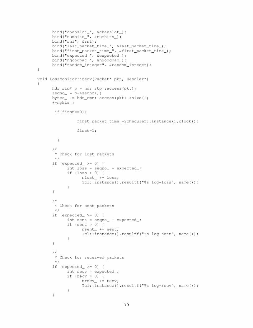
75

bind("chanslot_", &chanslot_);

bind("numhits_", &numhits_);

bind("rni", &rni);

bind("last_packet_time_", &last_packet_time_);

bind("first_packet_time_", &first_packet_time_);

bind("expected_", &expected_);

bind("ngoodpac_", &ngoodpac_);

bind("random_integer", &random_integer);

}

void LossMonitor::recv(Packet* pkt, Handler*)

{

hdr_rtp* p = hdr_rtp::access(pkt);

seqno_ = p->seqno();

bytes_ += hdr_cmn::access(pkt)->size();

++npkts_;

if(first==0){

first_packet_time_=Scheduler::instance().clock();

first=1;

}

/*

* Check for lost packets

*/

if (expected_ >= 0) {

int loss = seqno_ - expected_;

if (loss > 0) {

nlost_ += loss;

Tcl::instance().resultf("%s log-loss", name());

}

}

/*

* Check for sent packets

*/


int sent = seqno_ + expected_;

if (sent > 0) {

nsent_ += sent;

Tcl::instance().resultf("%s log-sent", name());

}

}

/*

* Check for received packets

*/


int recv = expected_;

if (recv > 0) {

nrecv_ += recv;

Tcl::instance().resultf("%s log-recv", name());

}

}

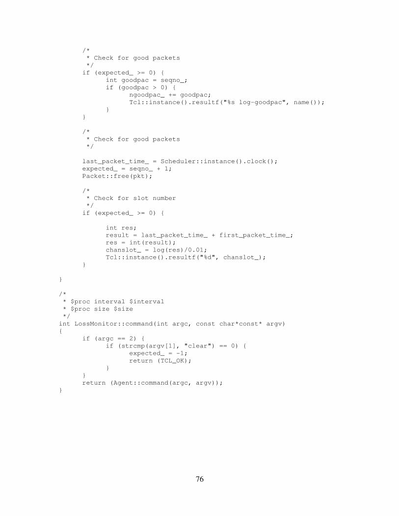
76

/*

* Check for good packets

*/


int goodpac = seqno_;

if (goodpac > 0) {

ngoodpac_ += goodpac;

Tcl::instance().resultf("%s log-goodpac", name());

}

}

/*

* Check for good packets

*/

last_packet_time_ = Scheduler::instance().clock();

expected_ = seqno_ + 1;

Packet::free(pkt);

/*

* Check for slot number

*/


int res;

result = last_packet_time_ + first_packet_time_;

res = int(result);

chanslot_ = log(res)/0.01;

Tcl::instance().resultf("%d", chanslot_);

}

}

/*

* $proc interval $interval

* $proc size $size

*/

int LossMonitor::command(int argc, const char*const* argv)

{

if (argc == 2) {

if (strcmp(argv[1], "clear") == 0) {

expected_ = -1;

return (TCL_OK);

}

}

return (Agent::command(argc, argv));

}

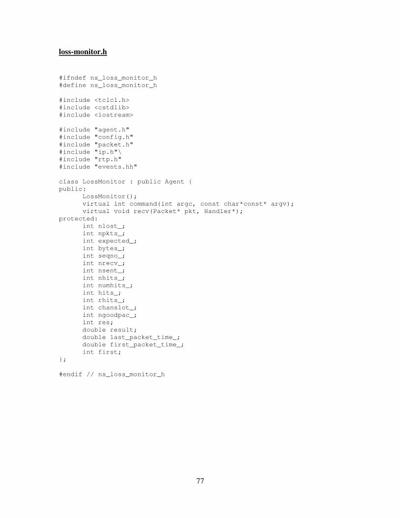
77

loss-monitor.h

#ifndef ns_loss_monitor_h

#define ns_loss_monitor_h

#include <tclcl.h>

#include <cstdlib>

#include <iostream>

#include "agent.h"

#include "config.h"

#include "packet.h"

#include "ip.h"\

#include "rtp.h"

#include "events.hh"

class LossMonitor : public Agent {

public:

LossMonitor();

virtual int command(int argc, const char*const* argv);

virtual void recv(Packet* pkt, Handler*);

protected:

int nlost_;

int npkts_;

int expected_;

int bytes_;

int seqno_;

int nrecv_;

int nsent_;

int nhits_;

int numhits_;

int hits_;

int rhits_;

int chanslot_;

int ngoodpac_;

int res;

double result;

double last_packet_time_;

double first_packet_time_;

int first;

};

#endif // ns_loss_monitor_h

Intelli MAC Layer Protocol for Cognitive Radio Networks

Documents

Transcript of Intelli MAC Layer Protocol for Cognitive Radio Networks