INTEGRATION OF OIL SANDS TAILINGS AND RECLAMATION PLANNING WITH LONG-

TERM MINE PLANNING

*M. M. Badiozamani1 and H. Askari-Nasab

2

1&2

University of Alberta

Department of Civil & Environmental Engineering

3-044 Markin/CNRL Natural Resources Engineering Facility (NREF)

9105 116th St, Edmonton, Alberta, Canada T6G 2W2

(*Corresponding author: mbadiozaman@ualberta.ca)

INTEGRATION OF OIL SANDS TAILINGS AND RECLAMATION PLANNING WITH LONG-TERM MINE

PLANNING

ABSTRACT

An optimized long-term mine planning determines the best order of material extraction, so that

the Net Present Value (NPV) becomes maximum. In the case of oil sands surface mining, one of the key

constraints in NPV maximization is the volume of tailings slurry that will be generated downstream.

Specifications of tailings slurry are also important from environmental perspective. Moreover, most of

the material that will be used for the reclamation of tailings ponds in later periods is generated in

extraction and processing of oil sands. In this paper, an integrated optimization framework is proposed to

maximize the NPV of the produced oil sands, with respect to tailings capacity constraints and reclamation

material requirements. A mixed integer linear programming (MILP) model is developed to find the

optimal solution for long-term mine planning problem. The proposed model is coded in Matlab and has

been run using CPLEX for verification. The results for real-case oil sands dataset show that the optimal

production schedule meets material requirements for reclamation, tailings volume is within tailings

capacity range in all periods and the production schedule follows the predetermined horizontal direction.

KEYWORDS

Mine planning, reclamation, tailings, mathematical programming, oil sands

INTRODUCTION

Open-pit mining is used to extract near-surface oil sands reserves in Northern Alberta. A mine

plan determines the best sequence of block extraction, the production schedule, in such a way to

maximize the NPV over the mine life. There are a number of downstream consequences associated with

any production schedule, such as the volume of tailings produced downstream as the result of bitumen

purification process. The extracted material is sent to the processing plant for further processing of

bitumen. There are environmental consequences associated with bitumen processing (Rodriguez, 2007;

Singh, 2008; Woynillowicz & Severson-Baker, 2009). Typically, tailings management is considered

separately from mine planning. In most of current practices, when the optimal mine plan is developed,

the volume of tailings is calculated and further decisions are made about sending the slurry to different

available tailings facilities. The volume and specifications of tailings is closely connected to the mining

operation and processing of the oil sands. Therefore, it is reasonable to include tailings management

considerations, such as tailings volume, as a set of constraints in the mine planning optimization model.

Oil sands operators must reclaim tailings ponds before leaving the mine site. Most of the

material that is used for reclamation comes from mining operations, such as over burden, oil sands

processing, or tailings coarse sand. When the mining project approaches to the mine closure, the

reclamation phase is planned in a way to make sure that the essential material for capping of tailings

ponds is available. It shows the connection between mining operations and reclamation material

requirement. Therefore, reclamation material requirement can also be integrated into the mine planning

model.

Long-term and short-term mine planning models maximize the NPV in strategic and operational

levels, respectively. In the literature, mine planning models for different time horizons are well

introduced (Askari-Nasab, Pourrahimian, Ben-Awuah, & Kalantari, 2011; Askari-Nasab, Tabesh, &

Badiozamani, 2010; Ben-Awuah & Askari-Nasab, 2011; Ben-Awuah, Askari-Nasab, & Awuah-offei, 2012).

Mine waste stream management and dyke construction for tailings dams is also included in mine planning

models (Odell, 2004; Rodriguez, 2007). There has also been research addressing environmental issues,

including reclamation costs in mine design(McFadyen, 2008). However, tailings management and

reclamation plans are not integrated in typical oil sands mine planning models and the merger between

these three research areas is the missing part in the literature. In this paper, the objective is to develop an

integrated long-term mine planning framework that maximizes the NPV and minimizes the reclamation

material handling costs at the same time. The integrated model includes tailings capacity constraints and

material requirements for tailings pond reclamation.

PROBLEM DEFINITION

To find the optimal production schedule that meets the tailings and reclamation requirements,

an integrated mine planning model must be developed. The inputs to this model are: (1) the optimal pit

limits that based on Lerch Grossman algorithm, determine which blocks are economically extractable, (2)

the block data, including spatial coordination of the blocks and the grade of different elements in each

block, and finally (3) a tailings model that determines the volume of tailings slurry, plus the volume of fine

material, sand and water resulted from extraction and processing of each block.

A sample reclamation plan that is published to fulfill the requirements of Directive 074 (Shell-

Canada, 2011) is a good example that shows the relation between the three concepts of long-term mine

planning, tailings management and reclamation planning. Shell Canada considers dedicated disposal

areas (DDA) for JackPine Mine (JPM) site at Athabasca river region in Alberta. Table 1 presents three main

steps that are included in decommissioning of an external tailings facility, including construction,

operations and closure. The time horizon in this decommissioning plan covers a period of 53 years,

between years 2008 and 2061 (Badiozamani & Askari-Nasab, 2012a).

Table 1 - Summary of JPM decommissioning time line

Construction (2008 to 2011):

• Preparation of Starter Dyke

• Preparation of External Dyke Walls (centerline)

• Preparation of Upstream Dyke

Operations (2010 to 2055):

• TT deposition – initial filing period

• Centrifuge Cake Manufacture / Deposition

• TT deposition – in-pit tailings CST capping activities (2)

• TT deposition – in-pit tailings CST capping activities

• TT deposition – in-pit tailings CST capping activities

• TFT transfer to SC1

Closure, Capping and Final Landform Design (up to 2055):

• Completion of TT deposition

• Trafficable tailings surface

• Overburden capping and drainage contouring reclamation cover soil

placement

• Nurse crop coverage and cap settlement

• Re-vegetation

• Monitoring

• Completion of TT deposition

All of the three phases of construction, operations and closure are influenced by the long-term

mine planning. Here are two instances that show how mine planning is important in decommissioning

phases; (1) waste material is required for starter dyke construction in construction phase. The mine

planning determines when and how much waste material is generated and can be used for reclamation.

(2) Thickened tailings (TT) and coarse sand tailings (CST) are required for filling and capping in operations

phase. Oil sands processing rate determines how much CST and TT is available in each period. The

processing rate is directly related to the amount of mineralized material that is sent to the processing

plant, determined in mine planning.

The reclamation plan proposed by Shell is just an example that shows the relation of mine

planning and reclamation plan. In general, with any change in the mine plan, the amount of waste that is

produced, as well as the volume of tailings slurry will be changed. Therefore, the reclamation plan must

consider such changes accordingly to make sure that the required material will be ready in right periods.

Knowing this fact, the objective of this paper is to develop an integrated strategic mine planning model

that maximizes the NPV over the mine-life, with respect to the capacity of tailings facility and material

requirement for tailings pond reclamation. In addition, a new term must be added to the objective

function to minimize the cost of materials handling for reclamation purposes. The organizations of a

typical model for mine planning (MILP-1) versus an integrated model (MILP-2) can be presented as:

MILP-1:

Maximize (NPV)

Subject to:

• Processing plant constraints

• Mining capacity constraints

• Extraction precedence constraints

MILP-2:

Maximize (NPV – reclamation costs)

Subject to:

• Processing plant constraints

• Mining capacity constraints

• Extraction precedence constraints

• Tailings capacity constraints

• Reclamation material requirement constraints

A schematic overview of integrated mine planning model is illustrated in Figure 1.

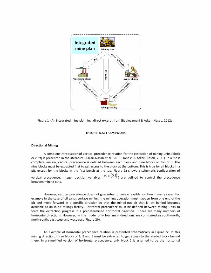
Figure 1 - An integrated mine planning, direct excerpt from (Badiozamani & Askari-Nasab, 2012a)

THEORETICAL FRAMEWORK

Directional Mining

A complete introduction of vertical precedence relation for the extraction of mining units (block

or cuts) is presented in the literature (Askari-Nasab et al., 2011; Tabesh & Askari-Nasab, 2011). In a most

complete version, vertical precedence is defined between each block and nine blocks on top of it. The

nine blocks must be extracted first to get access to the block at the bottom. This is true for all blocks in a

pit, except for the blocks in the first bench at the top. Figure 2a shows a schematic configuration of

vertical precedence. Integer decision variables ({ }0,1t

kb ∈) are defined to control the precedence

between mining-cuts.

However, vertical precedence does not guarantee to have a feasible solution in many cases. For

example in the case of oil sands surface mining, the mining operation must happen from one end of the

pit and move forward in a specific direction so that the mined-out pit that is left behind becomes

available as an in-pit tailings facility. Horizontal precedence must be defined between mining units to

force the extraction progress in a predetermined horizontal direction. There are many numbers of

horizontal directions. However, in this model only four main directions are considered as south-north,

north-south, east-west and west-east (Figure 2b).

An example of horizontal precedence relation is presented schematically in Figure 2c. In this

mining direction, three blocks of 1, 2 and 3 must be extracted to get access to the shaded block behind

them. In a simplified version of horizontal precedence, only block 2 is assumed to be the horizontal

predecessor for the shaded block behind (Figure 2d). It reduces the problem size and the implementation

results show that this is a valid assumption.

Figure 2 - Block precedence in vertical (a) and horizontal (b, c and d) directions, direct excerpt from

(Badiozamani & Askari-Nasab, 2012b)

To make large-scale problems solvable, mining blocks must be aggregated into mining-cuts

(Tabesh and Askari-Nasab, 2011). Mining-cuts do not have regular shapes and therefore, horizontal

precedence cannot be defined between them in the same way that is defined for mining blocks.

However, horizontal precedence relations are defined for mining-cuts based on the precedence relations

between mining blocks within the cuts.

Pushbacks are the backbone of long-term mine planning. They are typically defined as the

optimal pit limits (nested pits) resulted from increments in the revenue factors of the ore (bitumen).

Horizontal precedence can be defined among pushbacks in different ways. In this paper, the following

approach is used: if pushback 1 is predecessor of pushback 2 in a horizontal direction, then all the mining-

cuts at the very bottom of pushback 1 are considered as the predecessors for all the cuts at the top of

pushback 2. This will guarantee that extraction of mining-cuts in pushback 2 will not start before

completion of extraction of all the mining-cuts in pushback 1.

The Mixed Integer Linear Programming (MILP) Model

Mixed integer linear programming is used to formulate the long-term mine production

scheduling problem. Mining-cuts are used as the units of scheduling in MILP formulation framework

(Tabesh & Askari-Nasab, 2011). Different sets of continuous variables are defined to facilitate extraction

of ore portion, over/inter burden portion and tailings sand portion of each mining-cut and sending them

to various destinations, while binary variables are defined to control extraction precedence between

mining-cuts. The MILP has two objective functions, one for NPV maximization and the other one for cost

minimization associated with reclamation materials handling. The overall profit from mining and

processing of a mining-cut is proportional to the value of the cut and the total costs associated with

mining, processing and materials handling cost for reclamation at a specified destination. The

organization of the mathematical model is as follows:

Maximize

(NPV – reclamation material handling cost)

Subject to: Mining capacity constraints, Processing capacity constraints, Reclamation material requirement constraints, Total tailings capacity constraints, Limits for fines, sand and water in tailings, Quality of ore feed to the processing plant, Mass balance relations for different portions of cuts, Precedence constraints (vertical and horizontal)

Decision variables are defined in such a way that provides the required flexibility to the

optimizer for sending different portions of material for processing, reclamation or dumping as waste. The

concept of dynamic cut-off is used in construction of the MILP model, meaning that the optimizer

determines the destination of each parcel in such a way to maximize the NPV, rather than having a fixed

cut-off that predetermines material destination based on ore content of the parcels.

A complete formulation of the mathematical model including notation for sets, indices,

parameters, decision variables and the MILP model is presented in the appendix.

CASE STUDY

To verify the proposed MILP model, an oil sands dataset is used, that includes 45,648 blocks with

dimensions of 50 by 50 by 15 meters, in 9 benches. The mining blocks are aggregated into 478 larger units

as mining-cuts. The whole mine site is divided into two pushbacks, separated by a river. It is assumed that

pushback 1 proceeds pushback 2 in extraction. There are two destinations for the extracted material as:

(1) the processing plant, and (2) the waste dump. The problem is solved for 12 periods. Matlab

(MathWorksInc., 2011) is used for preparation of matrices for the objective function and the constraints.

The Matlab code calls TOMLAB/CPLEX (Holmström, Göran, & Edvall, 2009), which solves the mixed

integer linear programming model. The code is executed on a dual quad-core Dell Precision T7500

computer at 2.8 GHz, with 24GB of RAM. Some of the parameters for the case study are presented in

Table 2.

Figure 3 shows the grade distribution in the pushbacks. High-grade areas are shown in dark

colors (12% to 16%), while lighter patches represent low-grade material. To compare the NPV and decide

the best mining direction, the model is run for two directions of East-West (E-W) and West-East (W-E).

The Associated NPVs are compared in Table 3. The results show that mining in E-W direction generates a

better NPV, which is almost 10% better than the optimal solution in W-E direction.

As Figure 3 shows, the right part of the mine site (East) contains higher grade material,

comparing to the left (West). Therefore, it was expected to have a better NPV in E-W direction. Figures 4

and 5 present two sample plan views of resulted schedules for E-W and W-E directions, respectively.

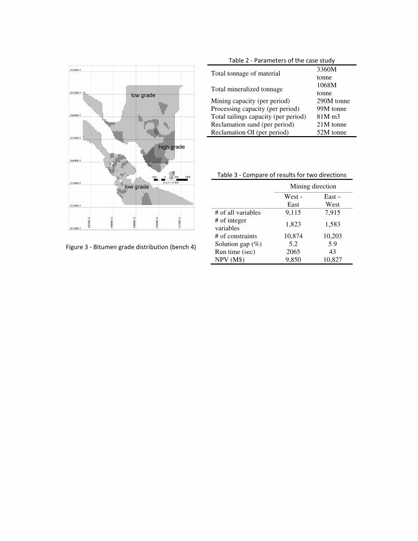
Figure 3 - Bitumen grade distribution (bench 4)

Table 2 - Parameters of the case study

Total tonnage of material 3360M tonne

Total mineralized tonnage 1068M tonne

Mining capacity (per period) 290M tonne Processing capacity (per period) 99M tonne Total tailings capacity (per period) 81M m3 Reclamation sand (per period) 21M tonne Reclamation OI (per period) 52M tonne

Table 3 - Compare of results for two directions

Mining direction

West - East

East – West

# of all variables 9,115 7,915 # of integer variables

1,823 1,583

# of constraints 10,874 10,203 Solution gap (%) 5.2 5.9 Run time (sec) 2065 43 NPV (M$) 9,850 10,827

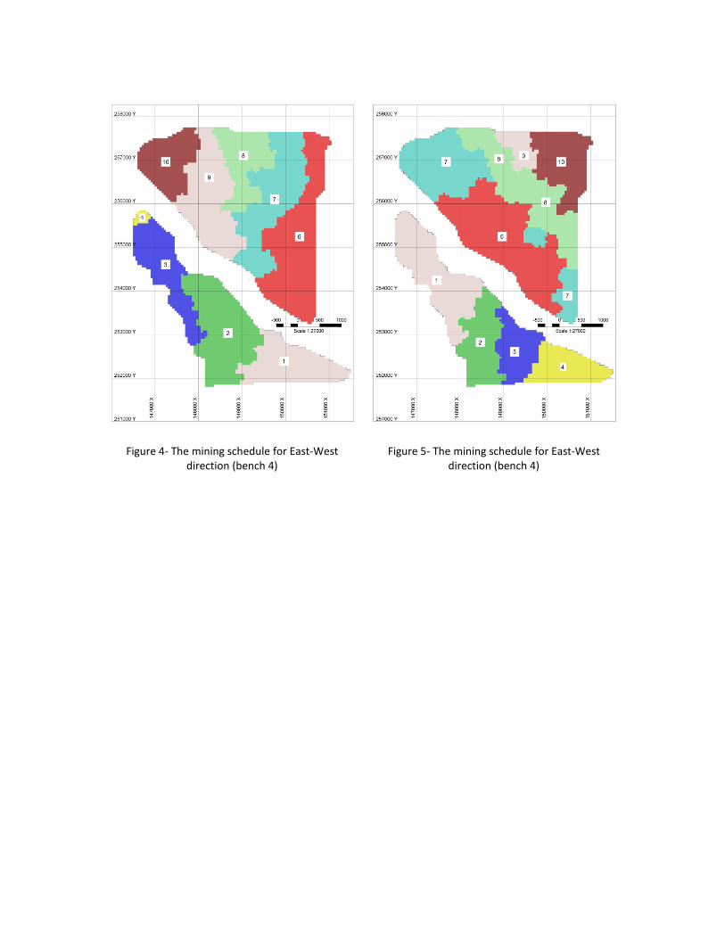
Figure 4- The mining schedule for East-West

direction (bench 4)

Figure 5- The mining schedule for East-West

direction (bench 4)

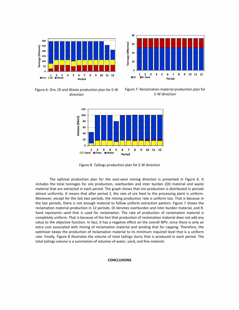
Figure 6- Ore, OI and Waste production plan for E-W

direction

Figure 7- Reclamation material production plan for

E-W direction

Figure 8- Tailings production plan for E-W direction

The optimal production plan for the east-west mining direction is presented in Figure 6. It

includes the total tonnages for ore production, overburden and inter burden (OI) material and waste

material that are extracted in each period. The graph shows that ore production is distributed in periods

almost uniformly. It means that after period 2, the rate of ore feed to the processing plant is uniform.

Moreover, except for the last two periods, the mining production rate is uniform too. That is because in

the last periods, there is not enough material to follow uniform extraction pattern. Figure 7 shows the

reclamation material production in 12 periods. OI denotes overburden and inter burden material, and R.

Sand represents sand that is used for reclamation. The rate of production of reclamation material is

completely uniform. That is because of the fact that production of reclamation material does not add any

value to the objective function. In fact, it has a negative effect on the overall NPV, since there is only an

extra cost associated with mining of reclamation material and sending that for capping. Therefore, the

optimizer keeps the production of reclamation material to its minimum required level that is a uniform

rate. Finally, Figure 8 illustrates the volume of total tailings slurry that is produced in each period. The

total tailings volume is a summation of volumes of water, sand, and fine material.

CONCLUSIONS

Near-surface oil sands reserves are extracted through open-pit mining. Mine planning

determines the optimal schedule for the extraction of the material in a way that maximizes the NPV.

Extraction and processing of oil sands generates huge volume of waste, mostly in form of slurry known as

tailings. One of the key factors that must be considered in mine planning is tailings management, because

of two facts: (1) the available area for tailings impoundment is limited to the lease area and this limitation

influences the mine planning indirectly, and (2) there are a number of environmental issues linked to the

tailings ponds and therefore, oil sands operators must reclaim the mine site and tailings ponds before

leaving the sites. These facts show that tailings management and reclamation planning must be

integrated into the mine planning to have a comprehensive mine plan. In this paper, an integrated mine

planning model is developed. It includes new sets of constraints for the capacity of tailings facility and the

requirements for reclamation material. For the tailings management, the total volume of tailings slurry,

plus the volumes of tailings components such as water, fine material and tailings coarse sand are

included. For reclamation material, the integrated mine planning model is constrained by preparing the

required tonnage of tailings coarse sand and over/inter burden material that will be used in later periods

for capping in reclamation phase. Moreover, a new term is added to the objective function that

minimizes the material handling cost of reclamation. An MILP model is developed for the integrated mine

planning problem. The model is verified by testing the solutions on a real-case oil sands dataset. The

results show that the optimal mine production schedule meets the tailings capacity constraints, as well as

the reclamation material requirements in each period. Two horizontal directions (W-E and E-W) are

compared to find the better mining direction for the case. As the next steps in this research, more

solution methods, such as Lagrangian relaxation algorithm will be investigated to improve the solution

time. Furthermore, in order to find the optimal solution for the large-scale problems in a reasonable time,

the model will be modified for different resolutions for the mining unit, as mining-blocks, mining-cuts,

and mining-panels.

REFERENCES

Askari-Nasab, H., Pourrahimian, Y., Ben-Awuah, E., & Kalantari, S. (2011). Mixed integer linear

programming formulations for open pit production scheduling. Journal of Mining

Science, 47(3), 338-359.

Askari-Nasab, H., Tabesh, M., & Badiozamani, M. M. (2010). Creating mining cuts using

hierarchical clustering and tabu search algorithms. Paper presented at the International

conference on mining innovation (MININ), Santiago, Chile.

Badiozamani, M. M., & Askari-Nasab, H. (2012a). Towards integration of oil sands mine planning

with tailings and reclamation plans. Paper presented at the Tailings and Mine Waste

2012, Keystone, Colorado, USA.

Badiozamani, M. M., & Askari-Nasab, H. (2012b). An integration of long-term mine planning,

tailings and reclamation plans. Paper presented at the International oil sands tailings

conference, Edmonton, AB, Canada.

Ben-Awuah, E., & Askari-Nasab, H. (2011). Oil Sands Mine Planning And Waste Management

Using Mixed Integer Goal Programming. International Journal of Mining, Reclamation

and Environment, 25(3), 226 - 247.

Ben-Awuah, E., Askari-Nasab, H., & Awuah-offei, K. (2012). Production scheduling and waste

disposal planning for oil sands mining using goal programming. Journal of environmental

informatics, International society for environmental information sciences, Regina,

Canada, Accepted on April 9, 2012, 37 pages.

Holmström, K., Göran, A. O., & Edvall, M. M. (2009). User's guide for TOMLAB /CPLEX (Version

12.1). Pullman, WA, USA: Tomlab Optimization Inc.

MathWorksInc. (2011). MATLAB Software (Version 7.13 (R2011b)).

McFadyen, D. (2008). Directive 074. Calgary: Energy Resources Conservation Board.

Odell, C. J. (2004). Integration of sustainability into the mine design process. Unpublished

Master of applied science, University of British Colombia, Vancouver.

Rodriguez, G. D. R. (2007). Evaluating the impact of the environmental considerations in open pit

mine design. Unpublished PhD., Colorado School of Mines, Golden.

Shell-Canada. (2011). Jackpine Mine: Dedicated disposal area (DDA) plan for DDA1 (TT Cell). Fort

McMurray, Alberta: Shell Canada Energy.

Singh, G. (2008, November 2008). Environmental impact assessment of mining projects. Paper

presented at the Proceedings of international conference on TREIA-2008, Nagpur.

Tabesh, M., & Askari-Nasab, H. (2011). A Two Stage Clustering Algorithm for Block Aggregation

in Open Pit Mines. Transactions of the Institution of Mining and Metallurgy, Section A:

Mining Technology, 120(3), 158-169.

Woynillowicz, D., & Severson-Baker, C. (2009). Oil sands fever: the environmental implications

of Canada's oil sands rush: The Pembina institute for appropriate development.

APPENDIX

The mixed integer linear programming model includes the following notation:

Sets

{ }1,..., KK = : Set of all mining cuts in the model.

{ }1,..., JJ = : Set of all phases (push-backs) in the model.

{ }1,...,UU = : Set of all material destinations in the model.

( )k

C L : For each mining-cut k, there is a set ( )k

C L ⊂ K defining the immediate predecessor mining-cuts

above mining-cut k that must be extracted prior to extraction of mining-cut k, where L is the total number

of mining-cuts in the set ( )k

C L .

( )kM P : For each mining-cut k, there is a set ( )k

M P ⊂ K defining the immediate predecessor mining-cuts

in a specified horizontal mining direction that must be extracted prior to extraction of mining-cut k at the specified level, where P is the total number of mining-cuts in the set ( )

kM P .

( )jB H : For each phase j, there is a set ( )jB H K⊂ defining the mining-cuts within the immediate

predecessor pit phases (push-backs) that must be extracted prior to extracting phase j, where H is an integer

number representing the total number of mining-cuts in the set ( )jB H .

Indices, Subscripts and Superscript

A parameter, f, can take indices, subscripts, and superscripts in the format, ,

,

u e t

k jf . Where:

{ }1,......,t T∈ : Index for periods.

{ }1,......,k K∈ : Index for mining-cuts.

{ }1,......,e E∈ : Index for elements of interest in each mining-cut.

{ }1,......,j J∈ : Index for phases (pushbacks).

{ }1,......,u U∈ : Index for material destinations.

, , ,D S M P : Subscripts and superscripts for overburden and inter burden material, tailings sand, mining and

processing respectively.

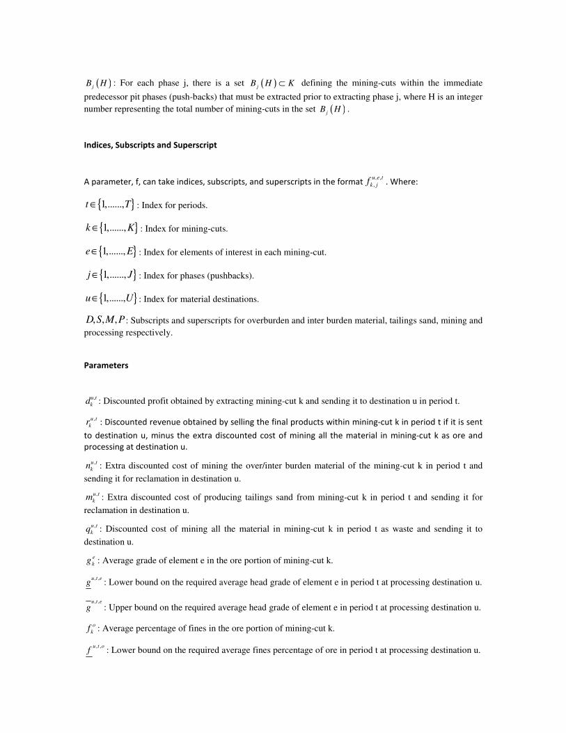
Parameters

,u t

kd : Discounted profit obtained by extracting mining-cut k and sending it to destination u in period t.

,u t

kr : Discounted revenue obtained by selling the final products within mining-cut k in period t if it is sent

to destination u, minus the extra discounted cost of mining all the material in mining-cut k as ore and

processing at destination u.

,u t

kn : Extra discounted cost of mining the over/inter burden material of the mining-cut k in period t and

sending it for reclamation in destination u.

,u t

km : Extra discounted cost of producing tailings sand from mining-cut k in period t and sending it for

reclamation in destination u.

,u t

kq : Discounted cost of mining all the material in mining-cut k in period t as waste and sending it to

destination u.

e

kg : Average grade of element e in the ore portion of mining-cut k.

, ,u t eg : Lower bound on the required average head grade of element e in period t at processing destination u.

, ,u t e

g : Upper bound on the required average head grade of element e in period t at processing destination u.

o

kf : Average percentage of fines in the ore portion of mining-cut k.

, ,u t of : Lower bound on the required average fines percentage of ore in period t at processing destination u.

, ,u t o

f : Upper bound on the required average fines percentage of ore in period t at processing destination u.

c

kf : Average percentage of fines in the over/inter burden reclamation material portion of mining-cut k.

, ,u t cf : Lower bound on the required average fines percentage of over/inter burden material in period t at

reclamation destination u.

, ,u t c

f : Upper bound on the required average fines percentage of over/inter burden material in period t at

reclamation destination u.

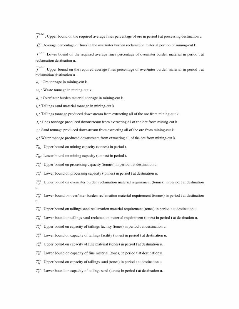
ko : Ore tonnage in mining-cut k.

kw : Waste tonnage in mining-cut k.

kd : Over/inter burden material tonnage in mining-cut k.

kl : Tailings sand material tonnage in mining-cut k.

kt : Tailings tonnage produced downstream from extracting all of the ore from mining-cut k.

kf : Fines tonnage produced downstream from extracting all of the ore from mining-cut k.

ks : Sand tonnage produced downstream from extracting all of the ore from mining-cut k.

kr : Water tonnage produced downstream from extracting all of the ore from mining-cut k.

t

MuT : Upper bound on mining capacity (tonnes) in period t.

t

MlT : Lower bound on mining capacity (tonnes) in period t.

,u t

PuT : Upper bound on processing capacity (tonnes) in period t at destination u.

,u t

PlT : Lower bound on processing capacity (tonnes) in period t at destination u.

,u t

CuT : Upper bound on over/inter burden reclamation material requirement (tonnes) in period t at destination

u.

,u t

ClT : Lower bound on over/inter burden reclamation material requirement (tonnes) in period t at destination

u.

,u t

NuT : Upper bound on tailings sand reclamation material requirement (tones) in period t at destination u.

,u t

NlT : Lower bound on tailings sand reclamation material requirement (tones) in period t at destination u.

,u t

TuT : Upper bound on capacity of tailings facility (tones) in period t at destination u.

,u t

TlT : Lower bound on capacity of tailings facility (tones) in period t at destination u.

,u t

FuT : Upper bound on capacity of fine material (tones) in period t at destination u.

,u t

FlT : Lower bound on capacity of fine material (tones) in period t at destination u.

,u t

SuT : Upper bound on capacity of tailings sand (tones) in period t at destination u.

,u t

SlT : Lower bound on capacity of tailings sand (tones) in period t at destination u.

,u t

WuT : Upper bound on capacity of tailings water (tones) in period t at destination u.

,u t

WlT : Lower bound on capacity of tailings water (tones) in period t at destination u.

,u er : Proportion of element e recovered (processing recovery) if it is processed at destination u.

,e tp : Price of element e in present value terms per unit of product.

,e tcs : Selling cost of element e in present value terms per unit of product.

, ,u e tcp : Extra cost in present value terms per tonne of ore for mining and processing at destination u.

,u tcl : Extra cost in present value terms for mining and shipping a tonne of over/inter burden material for

reclamation at destination u.

,u tcu : Extra cost in present value terms for mining and shipping a tonne of tailings sand material for

reclamation at destination u.

tcm : Cost in present value terms of mining a tonne of waste in period t.

Decision Variables

[ ], 0,1u t

kx ∈ : A continuous variable representing the portion of ore from mining-cut k to be extracted and

processed at destination u in period t.

[ ], 0,1u t

kw ∈ : A continuous variable representing the portion of OI material from mining-cut k to be

extracted and used for reclamation at destination u in period t.

[ ], 0,1u t

kv ∈ : A continuous variable representing the portion of tailings sand material from mining-cut k to

be extracted and used for reclamation at destination u in period t.

[ ]0,1t

ky ∈ : A continuous variable representing the portion of mining-cut k to be mined in period t, which

includes ore, over/inter burden material, tailings sand and waste.

[ ]0,1t

kb ∈ : A binary integer variable controlling the precedence of extraction of mining-cuts. t

kb is equal to

one if the extraction of mining-cut k has started by or in period t, otherwise it is zero.

[ ]0,1t

jc ∈ : A binary integer variable controlling the precedence of mining phases.

t

jc is equal to one if

the extraction of phase j has started by or in period t, otherwise it is zero.

Modeling of Economic Mining-Cut Value

, , , , ,u t u t u t u t u t

k k k k kd r q n m= − − −

{ } { } { }1,..., , 1,..., , 1,...,t T u U k K∀ ∈ ∈ ∈

Where:

( ), , , , , ,

1 1

E Eu t e u e e t e t u e t

k k k k

e e

r o g r p cs o cp= =

= × × × − − ×∑ ∑

{ } { } { }1,.., , 1,.., , 1,..,t T u U k K∀ ∈ ∈ ∈

( )t t

k k k kq o d w cm= + + ×

{ } { }1,.., , 1,..,t T k K∀ ∈ ∈

, ,u t u t

k kn d cl= × { } { } { }1,.., , 1,.., , 1,..,t T u U k K∀ ∈ ∈ ∈

, ,u t u t

k km l cu= × { } { } { }1,.., , 1,.., , 1,..,t T u U k K∀ ∈ ∈ ∈

The MILP Formulation

The objective functions of the MILP model for strategic and operational production plan for oil sands mining can be formulated as: i) maximizing the NPV and ii) minimizing the reclamation cost.

( ), ,

1 1 1 j

U T Ju t u t t t

k k k k

u t j k B

Max r x q y= = = ∈

× − ×

∑∑∑ ∑

( ), , , ,

1 1 1 j

U T Ju t u t u t u t

k k k k

u t j k B

Min n w m v= = = ∈

× + ×

∑∑∑ ∑

These two functions can be combined as a single objective function, formulated as:

( ), ,

, , , ,1 1 1 ( )j

u t u t t tU T J

k k k k

u t u t u t u tu t j k B

k k k k

r x q yMax

n w m v= = = ∈

× − × − × + ×

∑∑∑ ∑

The complete MILP model comprising of the combined objective function and constraints is formulated as:

Objective function:

( )

( )

, ,

, , , ,1 1 1 j

u t u t t tU T J

k k k k

u t u t u t u tu t j k B

k k k k

r x q yMax

n w m v= = = ∈

× − × − × + ×

∑∑∑ ∑

Subject to:

( )1 j

Jt t tMl k k k k Mu

j k B

T o w d y T

= ∈

≤ + + × ≤

∑ ∑

{ }1,...,t T∀ ∈

( ), , ,

1 j

Ju t u t u t

k PuPl k

j k B

T o x T

= ∈

≤ × ≤

∑ ∑

{ } { }1,..., , 1,...,t T u U∀ ∈ ∈

( ), , ,

1 j

Ju t u t u t

k CuCl k

j k B

T d w T

= ∈

≤ × ≤

∑ ∑

{ } { }1,..., , 1,...,t T u U∀ ∈ ∈

( ), , ,

1 j

Ju t u t u t

k NuNl k

j k B

T l v T

= ∈

≤ × ≤

∑ ∑

{ } { }1,..., , 1,...,t T u U∀ ∈ ∈

, ,, , , ,

1 j j

Ju t eu t e e u t u t

k k kk k

j k B k B

g g o x o x g

= ∈ ∈

≤ × × × ≤

∑ ∑ ∑

{ } { } { }1,.., , 1,.., , 1,..,t T u U e E∀ ∈ ∈ ∈

, ,, , , ,

1 j j

Ju t ou t o o u t u t

k k kk k

j k B k B

f f o x o x f

= ∈ ∈

≤ × × × ≤

∑ ∑ ∑

{ } { }1,.., , 1,..,t T u U∀ ∈ ∈

, ,, , , ,

1 j j

Ju t cu t c c u t u t

k k kk k

j k B k B

f f d w d w f

= ∈ ∈

≤ × × × ≤

∑ ∑ ∑

{ } { }1,.., , 1,..,t T u U∀ ∈ ∈

( ), , ,

1 j

Ju t u t u t

k TuTl k

j k B

T t x T

= ∈

≤ × ≤

∑ ∑

{ } { }1,..., , 1,...,t T u U∀ ∈ ∈

( ), , ,

1 j

Ju t u t u t

k FuFl k

j k B

T f x T

= ∈

≤ × ≤

∑ ∑

{ } { }1,..., , 1,...,t T u U∀ ∈ ∈

( ), , ,

1 j

Ju t u t u t

k SuSl k

j k B

T s x T

= ∈

≤ × ≤

∑ ∑

{ } { }1,..., , 1,...,t T u U∀ ∈ ∈

( ), , ,

1 j

Ju t u t u t

k WuWl k

j k B

T r x T

= ∈

≤ × ≤

∑ ∑

{ } { }1,..., , 1,...,t T u U∀ ∈ ∈

( ) ( ), ,

1

Uu t u t t

k k k k kk k

u

o x d w o d y

=

× + × ≤ + ×∑

{ } { }1,.., , 1,..,t T k K∀ ∈ ∈

( ) ( ), ,

1 1

U Uu t u t

k kk k

u u

l v o x

= =

× ≤ ×∑ ∑

{ } { }1,.., , 1,..,t T k K∀ ∈ ∈

,

1 1

1U T

u tk

u t

x

= =

≤∑∑

{ }1,..,k K∀ ∈

,

1 1

1U T

u tk

u t

w

= =

≤∑∑

{ }1,..,k K∀ ∈

,

1 1

1U T

u tk

u t

v

= =

≤∑∑

{ }1,..,k K∀ ∈

1

0t

t ik s

i

b y

=

− ≤∑

{ } { }1,..., , 1,..., , ( )kt T k K s C L∀ ∈ ∈ ∈

1

0t

t ik r

i

b y

=

− ≤∑

{ } { }1,..., , 1,..., , ( )kt T k K r M P∀ ∈ ∈ ∈

1

0t

i tk k

i

y b

=

− ≤∑

{ } { }1,..., , 1,...,t T k K∀ ∈ ∈

1 0t t

k kb b+

− ≤ { } { }1,..., 1 , 1,...,t T k K∀ ∈ − ∈

1

0t

t ij h

i

H c y

=

× − ≤∑

{ } { }1,..., , 1,..., , ( )jt T j J h B H∀ ∈ ∈ ∈

1

0t

i th j

i

y H c

=

− × ≤∑

{ } { } 11,..., , 1,..., , ( )jt T j J h B H+∀ ∈ ∈ ∈

1 0t tj jc c

+− ≤

{ } { }1,..., 1 , 1,...,t T j J∀ ∈ − ∈

1

1T

tk

t

y

=

=∑

{ }1,...,k K∀ ∈