1

Reprinted from: Journal of Geoscience Education, v. 46, 1998, p. 30-40.

Integrating Computers into the Field Geology CurriculumRoy Walter Schlische and Rolf Vincent AckermannDepartment of Geological SciencesRutgers University610 Taylor RoadPiscataway, New Jersey 08854-8066schlisch@rci.rutgers.edu

ABSTRACTThe Field Geology course at Rutgers University incor-porates computers in all projects, including the use ofan Electronic Total Station (ETS) and portable GlobalPositioning System (GPS) receivers in collecting fielddata. The ETS determines the distance and bearing tosighted points and calculates their spatial coordinatesand elevations; it then stores the results in a data-logger. GPS receivers provide absolute coordinates forstations occupied by the ETS itself or for outcrop loca-tions during mapping. The ETS is faster and more ac-curate than traditional surveying methods, and virtu-ally eliminates operator and transcription errors. Fur-thermore, ETS data can be downloaded directly to acomputer, where the data can be plotted, manipulated,and contoured.

We use the ETS/GPS system to collect topographicdata and map geologic contacts in a clay pit in the NewJersey coastal plain. Station locations are plotted andcontoured by computer. A computer-aided drafting(CAD) program is then used to put the finishing toucheson the geologic/topographic map. The ETS/GPS systemis also used to construct a detailed topographic map of astream channel and adjacent flood plain. Other com-puter applications include (1) using CAD programs todraw stratigraphic sections and to prepare presenta-tion-quality geologic maps; (2) using spreadsheet andgraphic programs to plot topographic profiles; and (3)using stereographic projection programs to plot andinterpret fracture data.

Keywords: GeologyÑField Trips and Field Study;EducationÑComputer Assisted

INTRODUCTIONThe use of computers in many aspects of geological

instruction has been increasing over the last decade. Anotable exception to this trend involves field methodscourses. This is unfortunate in that these courses arecommonly the capstone of the geology curriculum. Anycomputer applications that are used in field methodscourses rely on analysis, interpretation, and presenta-tion of data collected by conventional means in thefield. Consequently, the original data must be enteredinto the computer application by hand before any typeof analyses or interpretations may be undertaken. Inmany instances, this is unavoidable, in that there is noway to download the field data to a computer. A notableexample concerns spatial data collected by various sur-

veying equipment (alidades, theodolites, transits, auto-matic levels, etc.). The advent of Electronic Total Stations(ETS) and Global Positioning System (GPS) receivers nowmakes it possible to collect a wide range of spatial data inthe field, store the data in a data logging unit, and thendownload the data to a personal computer. This new tech-nology allows us to use computers in both the classroomand the field, where they will allow students to collect datamore quickly, easily, and reliably than was the case previ-ously. This will also afford the students more time to ana-lyze and interpret the data they have collected.

This year, we substantially revised the Field Geologycourse at Rutgers to incorporate computers in some aspectsof data collection and nearly all aspects of analysis andpresentation while retaining most of the traditional fieldtechniques (mapping on a topographic base and air photo,measuring stratigraphic sections, surveying with auto-matic levels and plane tables and alidades). In this paper,we present the Field Geology curriculum at Rutgers Uni-versity as an example of how computers can be integratedinto field courses. We also briefly describe the various com-puter applications used in this course, and present an ap-praisal of the merits and drawbacks of this approach.

The three-credit Field Geology course is required of allgeology majors who do not elect to attend an outside fieldcamp. Prerequisites include Sedimentology, Stratigraphy,and Structural Geology. The course is typically taken inthe senior year as the capstone of our curriculum and iscentered around a number of field-based projects whichstress active learning: students in small field groups (2-3students) must collect, analyze, and interpret field datautilizing a variety of field methods. The class meets foreight days prior to the start of the fall semester and thenfor six hours on Fridays for the first eight weeks of the se-mester. In the past five years, enrollments have rangedfrom 9 to 13 students, depending on how many students goaway to field camps.

The Field Geology syllabus is presented in Table 1.Computer applications fall into two broad types: (1) thoseused to manipulate, plot, and present geologic data ob-tained by traditional field methods, and (2) those used toobtain field data directly. In the following two sections, wedescribe these various computer applications with respectto the main Field Geology projects and also briefly describehow the field-based computer systems have been incorpo-rated in field projects in other geology courses. Here, welimit our discussion to Macintosh-based computer applica-tions; PC-based applications are briefly described in theDiscussion section.

2

Project Field Tasks Office TasksPreliminaryExercises

Pace-and-compass mapping of sidewalks onacademic quadrangle, Rutgers University

Plot pace-and-compass data using CANVASConstruct geologic maps from point data; pre-

pare cross sections

Godfrey Ridge

Tape-and-compass mapping of trail systemReconnaissance mapping of Godfrey Ridge and

Minisink Hills using topographic base & aer-ial photograph

Measured stratigraphic section, Minisink HillsStructural analysis of folds and minor struc-

tures at Interchange Quarry

Construct geologic map and cross sections onmylar

Draft stratigraphic section using CANVASDraft revised geologic map using CANVASWritten report

NewarkBasin

Reconnaissance mapping of Busch and Living-ston campuses on topographic base

Measured stratigraphic section, Douglass cam-pus

Collect joint orientation data, Busch andLivingston campuses

Project drill hole data to surfaceDraft geologic map using CANVASDraft geologic cross section (use of computers is

optional)Draft stratigraphic section using CANVASPlot fracture data using STEREONETWritten report

SayrevilleClay Pit

Use ETS/GPS to collect topographic and geo-logic data from SE wall of clay pit

Use plane table & alidade to collect topographicdata

Use automatic level to map lake marginMeasured stratigraphic section

Prepare topographic, geologic, and 3-D fishnetmap of ETS/GPS data using EXCEL,SURFACE, and CANVAS

Prepare topographic map of plane table datausing CANVAS and SURFACE

Plot stratigraphic section using CANVASWritten report

East BranchPerkiomenCreek

Use automatic level to measure profiles acrossstream channel

Use automatic level to transfer elevation fromknown benchmark to control points at profilelocations

Measure flow velocities and pebble b-axes; geo-logic characterization of channel and floodplain

Use ETS to map part of channel and floodplain

Plot topographic profiles of each transect usingCRICKETGRAPH and compare with profilesobtained during previous surveys

Prepare contour map of ETS data using EXCELand SURFACE

Use velocity and clast size data along withchannel geometry to perform various hydrau-lic calculations

Table 1: Field Geology curriculum as implemented in Fall 1995. Items in italics involve the use of computers.

USE OF COMPUTERS IN PLOTTING, MANIPULATING,AND PRESENTING FIELD DATAPreliminary Exercises

Following overview lectures on field procedures andmethodology on the first day of the course, students aregiven a relatively simple exercise in which they must pre-pare a pace-and-compass map of the walkways on the aca-demic quadrangle adjacent to the geology building. Stu-dents also use Bruntons, pace, and eye height to measurethe heights of light poles and the strike and dip of slopingsidewalks. Following data collection, students plot theirmaps using the drawing program CANVAS 3.5.4 (Deneba,1995) for the Macintosh. These preliminary exercises pro-vide the students with the opportunity to refamiliarizethemselves with the various uses of the Brunton compassand also provide a relatively straightforward introductionto the operation of CANVAS, which is routinely used in allField Geology projects. We also hand-out additional exer-cises on interpreting geologic map patterns, constructinggeologic cross sections, and constructing a geologic mapfrom "point data" that simulate outcrop stations utilized inactual geologic mapping.

Godfrey Ridge ProjectThis seven-day project takes place in the Valley and

Ridge Province near Stroundsburg and Delaware WaterGap, Pennsylvania. The study area consists of folded Silu-rian-Devonian limestones, sandstones, conglomerates, andshales (Epstein and Epstein, 1969; Epstein et al., 1967).Students are provided with an aerial photograph and pa-per copies of a topographic base map, which was scanned,digitized, and enlarged from the U.S.G.S. Stroudsburg andEast Stroudsburg 7.5" topographic quadrangle maps. AUniversal Transverse Mercator (UTM) grid has also beenadded to the base map, which provides a useful referenceframe for plotting stations whose coordinates were deter-mined with GPS receivers (see below). Students conducttape-and-compass traverses along a network of foot trails.CANVAS is used to prepare a map of the trails, which isthen printed out at the same scale as the base map. Stu-dents then manually trace the trails onto their copies ofthe base map. The trails provide a handy geographic refer-ence during mapping, which is conducted by studentsworking in pairs or triples during four days of field work.Additional field exercises involve measuring a detailedstratigraphic section through the contact between the

3

Oriskany Group and the Esopus Formation and analyzingthe structural relationships (cleavage-bedding relations,slickenlines related to flexural-slip folding, etc.) of a well-exposed fold in an old quarry.

Following the field work, students hand-draft theirmaps and cross sections on mylar or tracing paper. Afterthese maps are corrected and graded, students are pro-vided with CANVAS files containing the same topographicbase map they used in the field work. The students useCANVAS to draft and overlay a geologic map on the basemap. The geologic map includes formations and contacts,strike and dip symbols for bedding and cleavage, fold axialtraces, and a complete key (formations, ages, and descrip-tions as well as explanations of all structure symbols). Thefilled polygon tool is used to draft the formations and theircontacts (which can be either solid or dashed); the unfilledpolygon (polyline) tool is used in conjuction with arrowedlines to draft fold axial traces; using the azimuthal coordi-nate system in CANVAS, the line and text tools are used todraft strike and dip symbols. The final computer-draftedmaps are printed on a color printer. Students are gradedon the "correctness" of the geologic map and legend as wellas the overall quality of the presentation. The rationalebehind requiring students to prepare these computer-drafted maps is as follows: (1) students learn how to use acomputer drafting program to prepare presentation-qualitygeologic maps, and (2) in drafting these computer maps,the students have a chance to carefully observe (and hope-fully learn from) the mistakes that were made on thehand-drafted maps. Students also quickly learn that majorand minor changes can be made relatively quickly and eas-ily to their computer maps, e.g., changing colors of theformations, changing the map from color to grayscale orblack and white fill patterns, and enlarging or reducing theprinted dimensions of the map.

As part of the Godfrey Ridge project, students alsodraft their measured stratigraphic sections usingCANVAS. The ruler in CANVAS is set to the desired verti-cal scale of the stratigraphic column (e.g., 1 cm = 5 m).Rectangular objects representing the various stratigraphicunits can be quickly drafted. The heights of these rectan-gles can be easily adjusted to conform to the measuredthicknesses; the widths can also be adjusted to conform toa grain-size scale. These rectangles are given black andwhite fill patterns corresponding to the predominantlithology and are then stacked and left-aligned into a co-lumnar section. Special symbols for sedimentary struc-tures and fossils are easily added. Finally, descriptive text,scale, and legend are added to the columnar section (Fig-ure 1).

The final part of the project involves preparing a geo-logic report on the study area. These reports are edited forstyle, grammar, and content; graded; and returned to thestudents, who have the option of re-doing the written re-port for an improved grade.

Newark Basin ProjectThis three-day project involves outcrops of the Trias-

sic-Jurassic Newark basin located in and around the cam-puses of Rutgers University in New Brunswick and Pis-cataway, New Jersey. The goal of the mapping exercise is

to prepare a geologic map of the Busch and Livingstoncampuses. This area is underlain by the Passaic Forma-tion, which consists of predominantly red massive mud-stone but which also contains distinctive non-red markerunits. These non-red units have been identified in the Rut-gers drill hole (Olsen et al., 1996), and students use thesubsurface data to project the marker beds to the surface.Field mapping focuses on tracing these marker bedsthrough the study area. The marker beds are deformed bynormal faults and associated drag folds. Students plottheir field data on paper copies of a computer-drafted to-pographic base map, and then use CANVAS to draft theirgeologic maps on the digital base map. Many students alsouse CANVAS to draft their geologic cross sections. Stu-dents find that the zoom-in feature allows them to draftthe cross sections, which contain a large number of closelyspaced marker units, more carefully than is possible byhand.

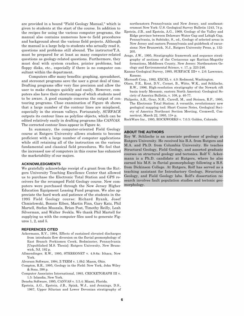
Students also measure a stratigraphic section of lakebeds displaying cyclical alternations in color and sedimentfabrics. Once again, CANVAS is used to draft the strati-graphic section. Students also measure a population ofjoints and use the program STEREONET 4.9.6a. (All-mendinger, 1995) to prepare scatter plots, Kamb contourplots, and rose diagrams (Figure 2). A written report inte-grating the drill core, map, fracture, and outcrop strati-graphic section data is also required.

USE OF COMPUTERS TO COLLECT FIELD DATAElectronic Total Station (ETS)

The ETS (Figure 3a) is a modern surveying instru-ment package (see Table 2 for list of equipment) that de-termines the distance to a rod-mounted reflecting prism(Figure 3b) using the travel time of reflected low-intensityinfrared laser light rays. The instrument (Fig. 3c) auto-matically calculates the horizontal distance and compassbearing to the prism as well as the change in elevationbetween the instrument and the sighted point, and canexpress these quantities in terms of relative or absolutecoordinates (e.g., northing, easting, and elevation; Table3). Corrections are automatically made for the curvature ofthe Earth and changes in the speed of light due to changesin temperature and barometric pressure. The range of theinstrument depends on the sophistication of instrumentand the ambient weather conditions. A basic unit (utlizingone prism) has a range of about 1 km. Precision is ±1.5mm; accuracy is ±5 mm.

Gun Environmental caseOptical plummet tribrach Rod with levelBattery charger Prism w/targetTripod ComputerPlumb bob Communications softwareFolding ruler StakesMounting bracket Spare batteriesData logger Walkie-TalkiesCable for connecting datalogger to gun

Cable from computer to datalogger

Table 2: List of ETS equipment.

4

Station Number Northing (ft) Easting (ft) Elevation (ft) Description

69 94680107 10160338 118 Topography70 94680614 10160381 182 Topography71 94680550 10160385 173 Base, Formation E72 94680502 10160386 165 Base, Formation A73 94680440 10160374 160 Base, Formation B74 94680359 10160381 145 Topography

Table 3: Sample ETS data.

About 4 seconds are required to take and store onemeasurement with the ETS. Data are stored in a data log-ging unit (Figure 3d); a basic unit can hold about 2500measurements. In addition to the spatial data, the datalogger also records station numbers and a brief descriptionof the station (up to 10 alphanumeric characters). Once setup, the ease and rapidity of operation allow the user tocover a large area rapidly or a small area in great detailrapidly. The data logging unit functions as an electronicfield notebook and thus eliminates the need for transcrib-ing data by hand, which eliminates associated human er-rors. Furthermore, because the instrument takes its ownreadings, there is no operator error, which is commonly thecase with other surveying instruments.

An important consequence of the faster surveying withthe ETS is the increased time it gives the user to concen-trate on geologic features. The ETS transforms detailedsurveying from a time-consuming, often frustrating proc-ess into a simple tool to be used by the field geologist.Given the speed with which data are collected with anETS, features such as geological contacts, outcrops, andcontours can be mapped as almost continuous lines withclosely spaced points, thus nearly eliminating the need forany freehand drawing (Philpotts et al., 1995).

The instrument always needs to know its location. Thecoordinates of the instrument's occupied point can be (1)determined using GPS receivers (see below), (2) arbitrarilyspecified, or (3) determined by shooting bearings to twoknown points. The instrument can be moved to new loca-tion after the coordinates of the new occupied point aredetermined by shooting a bearing to it.

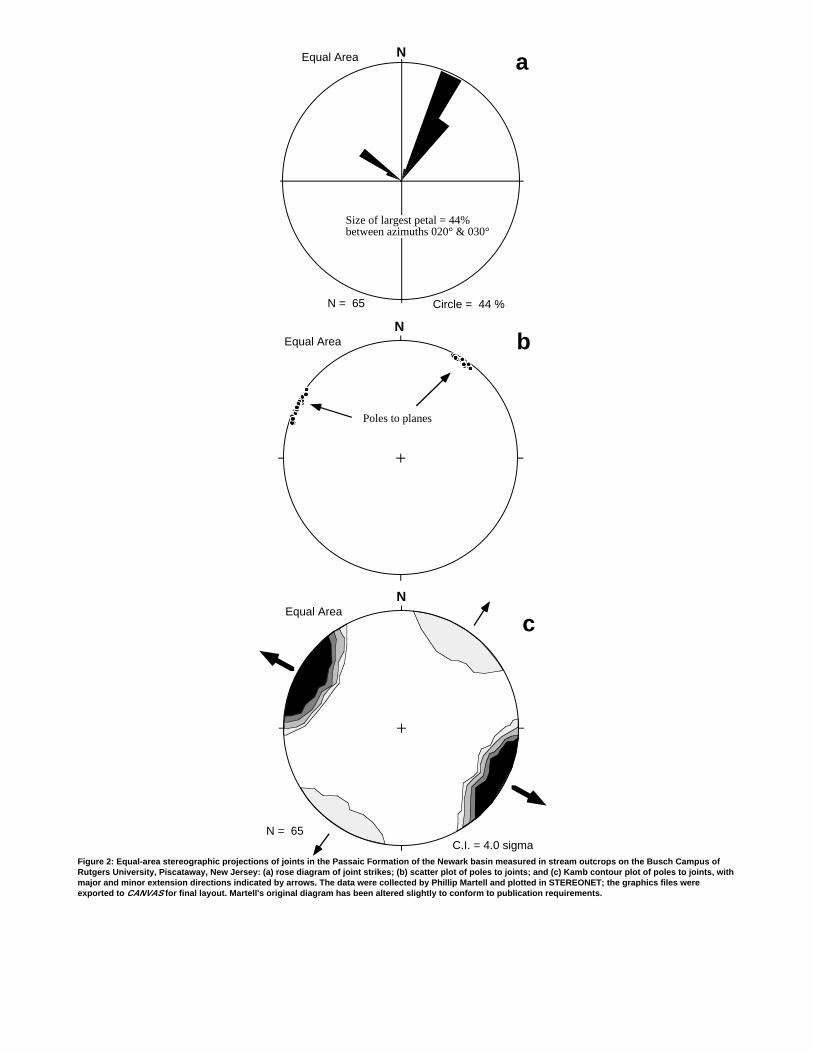
The data logging unit downloads its information di-rectly to a personal computer (Macintosh or PC) for subse-quent analyses, obviating the need to manually input thedata into other computer programs. We use the communi-cations program Z-TERM 1.0.2b (Alverson Software, 1994)to download from the data logger to a Macintosh. Thetransferred data files are saved as comma-delimited textthat can be read by the spreadsheet program EXCEL 4.0(Microsoft Corp., 1992). Data files can then be easily sortedand subdivided; for example, all stations occurring along agiven geologic contact can be saved as a separate file. Thedata files are then saved as text files, which can then beread by the plotting program SURFACE III+ v. 2.6 (Kan-sas Geological Survey, 1995). SURFACE can be used toprepare simple plots of station locations; station numbers,descriptions, or station elevations can be plotted next tothe station locations (Figure 4a). Various types of interpo-lated data grids and styles of topographic maps may begenerated from the elevation data (Figures 4b and 5). Mul-

tiple data files can be plotted on the same map, thus allow-ing stations along different contacts to be plotted usingdifferent symbols and/or colors (Figure 4b). The variousplots generated in SURFACE are then saved as PICT filesand exported into CANVAS, which can be used to "connectthe dots" for stations located along geologic contacts,faults, etc. Contouring errors (see discussion below) canalso be corrected at this stage. Structure symbols, legends,titles, etc. can also be added to the topographic/geologicmap (Figure 4c).

Global Positioning System (GPS)The Global Positioning System is based on 24 satel-

lites in geosynchronous orbit. It works by satellite rangingto a hand-held receiver, which computes its own position(e.g., latitude, longitude, and elevation) on the Earth. Thehand-held receivers (Figure 3e) work best in open areaswhere they have an unobstructed line of sight to multiplesatellites. Spatial locations can be supplied in lati-tude/longitude or Universal Transverse Mercator (UTM)coordinates. Errors associated with X-Y coordinates are upto 15 m (subject to U.S. Department of Defense 100 m se-lective availability) or up to 5 m if differential GPS serviceor a costly base station is used. Using the relatively inex-pensive hand-held receivers without a base station, eleva-tion (Z) data are not reliable. We use our GPS system todetermine X-Y coordinates of a benchmark or the initialoccupied location for the ETS. GPS units also accompanyus on the Godfrey Ridge and Newark basin mapping exer-cises and supply the students with the coordinates of criti-cal stations.

Sayreville ProjectThe field area for this two-day project is the Sayreville

Pit, an abondoned clay pit in the New Jersey CoastalPlain. Three Cretaceous stratigraphic units and Quater-nary alluvium are present in the study area (e.g., Jengo,1995). Erosion of the unconsolidated deposits has created abadlands topography, which is too detailed, complex, andchangeable to show on conventional 7.5" quadrangles. Stu-dents use the ETS and GPS systems to collect topographicdata within the quarry and to map the contacts betweenthe four geologic units. Electronic data files are down-loaded to a Macintosh, which is then used to prepare to-pographic and geologic maps using the programs EXCEL,SURFACE, and CANVAS as outlined above. SURFACE isalso used to prepare a 3-D topographic map (fishnet dia-gram) of the study area (Figure 5).

The Sayreville project also provides students with theopportunity to use other surveying equipment and to com-

5

pare these with the ETS system. Aside from the instruc-tional value, this is also necessary in that all studentscannot use the ETS system at once. An autolevel is used tomap out the perimeter of a lake that fills the center of thequarry; students are required to plot the lake shoreline byhand while in the field. A plane table and alidade is alsoused to obtain topographic data from a small part of thequarry. Station locations are plotted in their proper rela-tive positions directly in the field (e.g., Compton, 1985).These field maps are then optically scanned and importedinto CANVAS, within which it is easy to obtain the relativeX and Y coordinates of the stations--simply place the cur-sor over a station, and coordinates are displayed in a win-dow at the bottom of the screen. X, Y, and Z coordinatedata are then tabulated (by hand), entered in EXCEL, andthen transferred to SURFACE for plotting and contouring.Students are also given the option of contouring the eleva-tions by hand, but so far none has selected that option!

East Branch Perkiomen Creek ProjectThis project provides students with the opportunity to

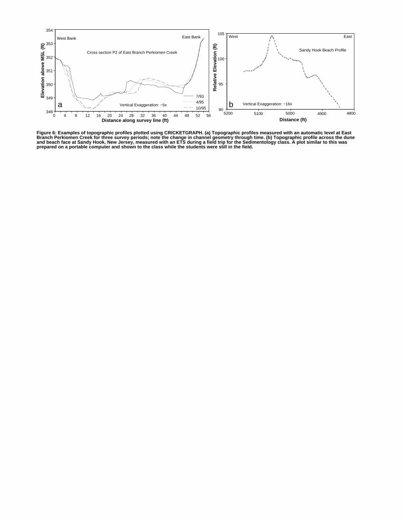
further use surveying equipment and to apply these skillsto study modern fluvial processes. The study area is lo-cated near the headwaters of East Branch PerkiomenCreek, near Bedminster, Pennsylvania. As a result of aflow-diversion project to supply cooling water to the Limer-ick Nuclear Generating Station, discharge within the creekhas been artificially elevated by up to 450% (Ackermann,1994) in summer months. Through repeated surveying ofthe same profiles, students have the opportunity to gaugeanthropogenically induced geomorphic changes. Elevationdata along four long-established cross sections are ob-tained by surveying with an automatic level. The topog-raphic data are plotted using CRICKETGRAPH III v. 1.5(Computer Associates, 1993) (Figure 6a). The ETS can alsobe used for this purpose, but because data collection, tran-scription, and data entry in CRICKETGRAPH are rela-tively rapid and easy, there is not much advantage to usingthe ETS. Furthermore, instrument setup is much morerapid for the autolevel than for the ETS. Instead, the ETSsystem is used to obtain detailed topographic data of a partof the channel and adjacent floodplain. The data are plot-ted and contoured using SURFACE. The plots are thenimported to CANVAS for final touch-up.

Other tasks performed during this exercise include: (1)transferring elevations from a benchmark to the localbenchmarks present at each of the four transects using anautomatic level; (2) measuring flow velocities with a cur-rent meter; and (3) measuring b-axes of pebbles (studentsenter the clast size data in EXCEL, sort it, and then readoff the values of the 16th, 50th, and 84th percentiles). In awritten report, students assess the amount of geomorphicchange over time and use hydraulic equations to calculatedischarge, Froude number, Reynolds number, shearstresses, and the maximum clast sizes that can be en-trained by the flow.

Use of ETS and GPS in Other CoursesIn addition to the Field Geology course, we have also

used the ETS on field trips for the Sedimentology and In-troduction to Geophysics courses. The ETS was used atSandy Hook, New Jersey, to measure a beach profile and

to construct a topographic map of the beach. ETS datawere then downloaded to a Macintosh Powerbook computerwhile we were still in the field. The beach profile was thenplotted using CRICKETGRAPH (Figure 6b). The signifi-cance of this profile was discussed with the students whilewe were still at the beach! The Introduction to Geophysicsclass obtained a series of seismic refraction profiles acrosspart of Rutgers' Busch Campus. The ETS was used to de-termine the relative elevations of all the geophone loca-tions so that a statics correction could be made to the two-way travel-time data.

DISCUSSIONAt the end of 1995 Field Geology course, all students

received a detailed questionnaire about the content andworkload of the course. Six of 11 students returned theevaluations. The discussion below is based on the results ofthe evaluation and our own observations and impressions.

Students appreciate being able to learn more aboutusing computers. However, the use of computers in a FieldGeology course should not reduce the number of field exer-cises. Furthermore, if computers are to be successfullyused in a field geology course, they must be an integralpart of data collection, manipulation, and/or presentation.In addition, the required task should generally be easierand/or faster to do on the computer than by other means. Ifnot, students must be told explicitly the advantages of us-ing the computers (e.g., a digital map can be printed atalmost any size; it is easy to make changes; the output isoften publication-quality). Students dislike exercises thatthey feel are repetitive (e.g., measuring and drafting threestratigraphic sections). We plan to revise our course bydeleting one of the stratigraphic sections and giving thestudents a choice of drafting the Newark basin geologicalmap by hand or on the computer.

Computer facilities must be adequate to allow all stu-dents the opportunity to complete the required exercises,especially during crunch time (the evening before an as-signment is due). Given that students overwhelmingly pre-fer Macintoshes to PC's, the number of Macintoshes in ourdepartmental computer room (6) was barely adequate forthe number of students (11). When students elected to usea PC, the four in our computer room were adequate.

We believe that is important to allow students tochoose between Macintoshes and PC's. Perhaps even moreimportantly, we believe that students should be familiarwith both platforms. In order to encourage greater utliza-tion of the PC's, we have selected programs that are simi-lar on both platforms. With respect to CANVAS, our mostheavily utilized program, the PC and Mac versions arevirtually identical, and files can be exchanged across plat-forms; the same is true for EXCEL. Although not identicalto SURFACE, Gridzo in ROCKWORKS (RockWare, 1995)provides plotting and contouring options for the PC.

Many students are unfamiliar with the basic operationof computers, and require preliminary training. Some ofthis is provided in other courses. At Rutgers, we now usecomputer exercises in Sedimentology, Stratigraphy, Pe-trology, Structural Geology, and Geophysics, as well asGeological Modeling (an optional course). Nonetheless, thestudents do still require detailed instructions on the proce-dures for using the various computer applications. These

6

are provided in a bound "Field Geology Manual," which isgiven to students at the start of the course. In addition tothe recipes for using the various computer programs, themanual also contains numerous how-to field proceduresand background about the various field projects. Althoughthe manual is a large help to students who actually read it,questions and problems still abound. The instructor/T.A.must be prepared for at least as many computer-relatedquestions as geology-related questions. Furthermore, theymust deal with system crashes, printer problems, badfloppy disks, etc., especially if there is no computer con-sultant within the department.

Computers offer many benefits: graphing, spreadsheet,and stereonet programs save the user a great deal of time.Drafting programs offer very fine precision and allow theuser to make changes quickly and easily. However, com-puters also have their shortcomings of which students needto be aware. A good example concerns the output of con-touring programs. Close examination of Figure 4b showsthat a large number of the contour lines are misplaced,especially in the stream valleys. Fortunately, SURFACEoutputs its contour lines as polyline objects, which can beedited relatively easily in drafting programs like CANVAS.The corrected contour lines appear in Figure 4c.

In summary, the computer-oriented Field Geologycourse at Rutgers University allows students to becomeproficient with a large number of computer applicationswhile still retaining all of the instruction on the variousfundamental and classical field procedures. We feel thatthe increased use of computers in this course has enhancedthe marketability of our majors.

ACKNOWLEDGMENTSWe gratefully acknowledge receipt of a grant from the Rut-gers University Teaching Excellence Center that allowedus to purchase the Electronic Total Station and GPS re-ceivers for the revamped Field Geology course. New com-puters were purchased through the New Jersey HigherEducation Equipment Leasing Fund program. We also ap-preciate the hard work and patience of the students in the1995 Field Geology course: Richard Byank, JosefChmielowski, Bonnie Eiben, Martin Finn, Gary Katz, PhilMartell, Stefan Muszala, Brian Post, Timothy Reilly, LeahSilverman, and Walter Svekla. We thank Phil Martell forsupplying us with the computer files used to generate Fig-ures 1, 2, and 5.

REFERENCES CITEDAckermann, R.V., 1994, Effects of sustained elevated discharges

from intrabasin flow diversion on the fluvial geomorphology ofEast Branch Perkiomen Creek, Bedminster, Pennsylvania[Unpublished M.S. Thesis]: Rutgers University, New Bruns-wick, NJ, 192 p.

Allmendinger, R.W., 1995, STEREONET v. 4.9.6a: Ithaca, NewYork.

Alverson Software, 1994, Z-TERM v. 1.0b2: Mason, Ohio.Compton, R.R., 1995, Geology in the Field: New York, John Wiley

& Sons, 398 p.Computer Associates International, 1993, CRICKETGRAPH III v.

1.5: Islandia, New York.Deneba Software, 1995, CANVAS v. 3.5.4: Miami, Florida.Epstein, A.G., Epstein, J.B., Spink, W.J., and Jennings, D.S.,

1967, Upper Silurian and Lower Devonian stratigraphy of

northeastern Pennsylvania and New Jersey, and southeast-ernmost New York: U.S. Geological Survey Bulletin 1243, 74 p.

Epstein, J.B., and Epstein, A.G., 1969, Geology of the Valley andRidge province between Delaware Water Gap and Lehigh Gap,Pennsylvania, in Subitzky, S., ed., Geology of selected areas inNew Jersey and eastern Pennsylvania and guidebook of excur-sions: New Brunswick, N.J., Rutgers University Press, p. 132-205.

Jengo, J.W., 1995, Stratigraphic framework and sequence strati-graphy of sections of the Cretaceous age Raritan-Magothyformations, Middlesex County, New Jersey: Northeastern Ge-ology and Environmental Science, v. 17, p. 223-246.

Kansas Geological Survey, 1995, SURFACE III+ v. 2.6: Lawrence,Kansas.

Microsoft Corp., 1992, EXCEL v. 4.0: Redmond, Washington.Olsen, P.E., Kent, D.V., Cornet, B., Witte, W.K., and Schlische,

R.W., 1996, High-resolution stratigraphy of the Newark riftbasin (early Mesozoic, eastern North America): Geological So-ciety of America Bulletin, v. 108, p. 40-77.

Philpotts, A.R., Gray, N.H., Carroll, M., and Steinen, R.P., 1995,The Electronic Total Station: A versatile, revolutionary newgeological mapping tool: Short Course Notes, Geological Soci-ety of America Northeast Section Meeting, Cromwell, Con-necticut, March 22, 1995, 13+ p.

RockWare Inc., 1995, ROCKWORKS v. 7.0.5: Golden, Colorado.

ABOUT THE AUTHORSRoy W. Schlische is an associate professor of geology atRutgers University. He received his B.A. from Rutgers andM.A. and Ph.D. from Columbia University. He teachesStructural Geology, Field Geology, and assorted graduatecourses on structural geology and tectonics. Rolf V. Acker-mann is a Ph.D. candidate at Rutgers, where he alsoearned his M.S. in fluvial geomorphology following a B.S.from Dickinson College. At Rutgers, Rolf has served as ateaching assistant for Introductory Geology, StructuralGeology, and Field Geology labs. Rolf's dissertation re-search involves fault population studies and tectonic geo-morphology.

.

500

600

Composite Columnar Section Along Minisink Hills, Monroe County, Pennsylvania

Graphiccolumnar section

Description

1.0

2.0

3.0

4.0

5.0

6.0

7.0

8.0

9.0

10.0

11.0

12.0

13.0

14.0

15.0

16.0

17.0

18.0

19.0

20.0

21.0

22.0

23.0

24.0

25.0

26.0

27.0

28.0

0

X

XN 41° 00'00''W 075° 08'31''

=

F.G. qtz ss. Chert nodules and layerspresent. Weathered light brown, fresh gray.

Covered interval

Black chert bed, fine grained.C.G. qtz ss, clasts~0.5 - 5.0 mm.F.g. qtz ss with chert nodules. Lt. gray

Fe staining.

F.G. ss, cleavage present, chert nodules parallel to bedding.Buff/gray color.

Qtz cong. clasts ~ 1.0 - 7.0mm. Clast supported.F.G. ss. Clasts uniform in size.

C.G. qtz ss, grains well rounded, HCl rxn, clasts ~ 0.5 - 5.0mm.F.G. qtz ss, HCl rxn, random clasts ~ 2.0mm.

C.G. qtz ss. Clasts well rounded, HCl rxn, Fe stained.

F.G. S.S. HCl rxn.C.G. clast supported, qtz ss. CaCO3 matrix, grains translucent.

Cong. qtz ss. Clasts are rounded to sub - rounded.M.G qtz ss. Clasts fine upward and are sub - rounded.

M.G. - F.G. qtz ss. Clast supported,wormy looking holes in bed.

Conglomeratic ss. Clasts ~ 5.0 mm Sub - horizontal jointingpresent throughout layer. HCl rxn.

Covered interval

Moss-covered limey shale. Silt sized grains are HCl reactive.

Shale with interbedded chert nodules. Brachiopods present.

Fe stained shale. Brachiopods and other fossils present.

Covered interval

Well-laminated , dark gray shale. Fe staining and cleavageprominant.

Key

Based on 1:24000 Stroudsburg(1973) and East Stroudsburg

(1993) USGS Topo Quads

By Phillip Martell and Josef ChmielowskiSeptember 1, 1995

Measured with a tape measure

F.G. - Fine grained

M.G. - Medium grained

C.G. - Coarse grained

ss - Sandstone

Cong - Conglom- eraticRxn - Reaction

Sandstone

Conglomerate

Shale

Laminatedshale

Limey shale

Chert

Quartz clast

Burrow

Brachiopod

Fossil

Chert nodule

22.0

8

Ori

skan

y G

roup

Eso

pus

Form

atio

n

5.07

Feet

abov

e ba

se

Thi

ckne

ssin

fee

t

Form

atio

n

Seri

esL

ower

Dev

onia

n10.5°

MN N

F.G. ss, well sorted with CaCO3 matrix. Fossils present.Gray-green color.

Figure 1: Stratigraphic section prepared by Phillip Martell using CANVAS as part of the Godfrey Ridge project. Thesection was measured by Martell and Josef Chmielowski. Martell's original diagram has been altered slightly toconform to publication requirements.

Equal Area

N = 65C.I. = 4.0 sigma

N

c

Equal Area

Poles to planes

N

N = 65 Circle = 44 %

Equal Area

Size of largest petal = 44%between azimuths 020° & 030°

N a

b

Figure 2: Equal-area stereographic projections of joints in the Passaic Formation of the Newark basin measured in stream outcrops on the Busch Campus ofRutgers University, Piscataway, New Jersey: (a) rose diagram of joint strikes; (b) scatter plot of poles to joints; and (c) Kamb contour plot of poles to joints, withmajor and minor extension directions indicated by arrows. The data were collected by Phillip Martell and plotted in STEREONET; the graphics files wereexported to CANVAS for final layout. Martell's original diagram has been altered slightly to conform to publication requirements.

Figure 3: (a) Bonnie Eiben looking through the gun of an ETS in the Sayreville Pit, Sayreville, New Jersey. (b)Walter Svekla holding rod-mounted prism and walkie-talkie in the Sayreville Pit. (c) Closeup view of the gun andoptical tribrach. The LCD display of the gun shows the current vertical angle (measured from the vertical) andhorizontal azimuth (measured with respect to north) in degrees, minutes, and seconds. (d) Closeup view of thedata logger. Within the LCD display: OC refers to occupied point (the current location of the gun and tripod) andgives its station number; FS refers to front sight (a station surveyed by the ETS) and gives its station number ;BS refers to back sight (a station used to establish the position of the occupied point) and gives its station num-ber; azimuth is the horizontal angle in degrees, minutes, seconds (DD.MMSS) from the OC to the current FS);Zenith ang is the vertical angle (in DD.MMSS ) between OC and FS; slope dist. is the distance (in feet) betweenOC and FS; Desca is a description of station 1376; HI is the height of the instrument (in feet); and HR is theheight of the rod (in feet). Operations are key- and menu-driven. (e) Closeup of GPS receiver. Under "POSITION",the instrument displays the UTM coordinates of a station (Edison, New Jersey) within Zone 18T .

.

196.

195.

192.

192.

188.

186.

185.

183.

180.

166.

195.

193.

188.

188.

185.

180.

180.

180.

170.

155.

193.

185.

180.

184.

185.

173.

160.

155.

150.

190.

185.

181.

173.

173.

182.

181.

173.

145.

145.

141.

187.

183.

173.

155.

165.

165.

160.

135.

150.

135.

133.

188.

185.

182.

173.

155.

150.

147.

140.

128.

125.

185.

180.

165.

150.

140.

138.

120.

118.

182.

173.

165.

160.

145.

128.

130.

120.

114.

185.

173.

155.

150.

135.

125.

124.

115.

112.

190.

185.

180.

173.

155.

146.

130.

123.

116.

113.

109.

190.

185.

185.

173.

155.

146.

131.

120.

113.

110.

106.

188.

185.

173.

160.

153.

145.

130.

120.

113.

105.

103.

188.

182.

155.

145.

135.

125.

115.

110.

103.

185.

180.

173.

155.

140.

125.

115.

108.

103.

173.173.

173.

173.

173.

173.

173.

173.

173.

173.

173.

173.

173.

165.

155.145.

135.140.

150.

165.155.

170.

185.

145.

115.

110.

180.

150.

130.

117.

110.

160.

145.

110.

125.

160.

94680096.

94680144.

94680192.

94680240.

94680288.

94680336.

94680384.

94680432.

94680480.

94680528.

94680576.

94680624.

189.

184.

175.

155.

140.

127.

117.

108.

103.

173.

94680096.

94680144.

94680192.

94680240.

94680288.

94680336.

94680384.

94680432.

94680480.

94680528.

94680576.

94680624.

10160650.10160550.10160450.10160350.10160250.10160150.10160100.10160050.

10160200. 10160300. 10160400. 10160500. 10160600. 10160700.

196.

195.

192.

192.

188.

186.

185.

183.

180.

166.

195.

193.

188.

188.

185.

180.

180.

180.

170.

155.

193.

185.

180.

184.

185.

173.

160.

155.

150.

190.

185.

181.

173.

173.

182.

181.

173.

145.

145.

141.

187.

183.

173.

155.

165.

165.

160.

135.

150.

135.

133.

188.

185.

182.

173.

155.

150.

147.

140.

128.

125.

185.

180.

165.

150.

140.

138.

120.

118.

182.

173.

165.

160.

145.

128.

130.

120.

114.

185.

173.

155.

150.

135.

125.

124.

115.

112.

190.

185.

180.

173.

155.

146.

130.

123.

116.

113.

109.

190.

185.

185.

173.

155.

146.

131.

120.

113.

110.

106.

188.

185.

173.

160.

153.

145.

130.

120.

113.

105.

103.

188.

182.

173.

155.

145.

135.

125.

115.

110.

103.

185.

180.

173.

155.

140.

125.

115.

108.

103.

173.173.

173.

173.

173.

173.

173.

173.

173.

173.

173.

173.

173.

165.

155.

145.

135.140.

150.

165.155.

170.170.

165.

155.

163.

170.

185.

145.

115.

110.

180.

150.

130.

117.

110.

160.

145.

110.

125.

160.

189.

184.

175.

155.

140.

127.

117.

108.

103.

173.

Base, Formation A

Base, Formation B

Base, Formation CBase, Formation E

a

b10160650.10160550.10160450.10160350.10160250.10160150.10160100.

10160050.10160200. 10160300. 10160400. 10160500. 10160600. 10160700.

Figure 4: Example of how ETS-like data can be used to prepare a topographic and geologic map using SURFACE andCANVAS. To prepare this figure, a hypothetical topographic/geologic map was first drafted in CANVAS. The X, Y, and Zcoordinates for 190 "stations" were read off in CANVAS (for real-world examples, the ETS would obtain this data),entered in EXCEL, and then transferred to SURFACE. (a) Posting map of the stations with elevations; grid numberssimulate a UTM-type grid. (b) Contour map of elevation data from (a). Also shown with different symbols are stationslocated along geologic contacts. This diagram was then exported to CANVAS.

94680096

94680144

94680192

94680240

94680288

94680336

94680384

94680432

94680480

94680528

94680576

94680624

175

175

175

175

150

125

Lake

Te

Te

Ka

Kb

Kc

Kd

N 0 25 50 75 100 ft

0 10 20 30 m

Contour interval: 5 ft.Easting (ft.)

No

rth

ing

(ft

.)

Te

Kd

Kc

Kb

Ka

Formation E

Formation D

Formation C

Formation B

Formation ACre

tace

ous

Ter

tiary

c

10160650.10160550.10160450.10160350.10160250.10160150.10160100.10160050.

10160200. 10160300. 10160400. 10160500. 10160600. 10160700.

150

Figure 4, continued: (c) Final topographic/geologic map prepared using CANVAS: contour lines were corrected; thepolygon tool was used to "connect the dots" of stations located along contacts and to show the areal extent of thefive formations; a scale and legend were added.

220 meters

165 meters

V.E. = 20x

0554950.00 4779400.00

4479190.00

0555120.00

MNN

12°

Three Dimensional View of the Sayreville Pit, Sayreville,Middlesex County, New Jersey

by Phillip J. MartellOctober 1995 = Study Area

1000 Meters

Topographic data collected by the 1995 RutgersField Geology class using an Electronic Total

Station

Coordinates are in UTMcoordinates from GPS

receiver, Zone 18

Elevations relative toarbitrary 100m

benchmark

No Data

Figure 5: Three-dimensional perspective (fishnet) diagram illustrating the topography of the southeast wall of the Sayreville Pit.Topographic data were collected using an ETS and were plotted by Phillip Martell using SURFACE and CANVAS. Martell's originaldiagram has been altered slightly to conform to publication requirements.

348

349

350

351

352

353

354

0 4 8 12 16 20 24 28 32 36 40 44 48 52 56Distance along survey line (ft)

Cross section P2 of East Branch Perkiomen Creek

10/95

4/957/93

West Bank East BankE

leva

tio

n a

bo

ve M

SL

(ft

)

a Vertical Exaggeration: ~5x90

95

100

105West East

5200 5100 5000 4900 4800

Vertical Exaggeration: ~16x

Distance (ft)

Rel

ativ

e E

leva

tio

n (

ft)

b

Sandy Hook Beach Profile

Figure 6: Examples of topographic profiles plotted using CRICKETGRAPH. (a) Topographic profiles measured with an automatic level at EastBranch Perkiomen Creek for three survey periods; note the change in channel geometry through time. (b) Topographic profile across the duneand beach face at Sandy Hook, New Jersey, measured with an ETS during a field trip for the Sedimentology class. A plot similar to this wasprepared on a portable computer and shown to the class while the students were still in the field.