Integrated Model - 国立環境研究所 · 2018-09-05 · AIM Enduse Model Manual . AIM Interim...

AIM Enduse Model Manual

Integrated Model

Asia-Pacific

AIM

AIM Interim Report2015

AIM Enduse Model Manual AIM Interim Report 2015

Authors

Tatsuya Hanaoka* : National Institute for Environmental Studies

Contact: [email protected]

Toshihiko Masui : National Institute for Environmental Studies

Yuzuru Matsuoka : Kyoto University

Go Hibino : Mizuho Information & Research Institute

Kazuya Fujiwara: Mizuho Information & Research Institute

Yuko Motoki: Mizuho Information & Research Institute

Ken Oshiro: Mizuho Information & Research Institute

* Editor of this report

Content

1. Overview of AIM/Enduse ............................................................................................................. 1 1.1 What is AIM/Enduse? ........................................................................................................... 1

1.1.1 Characteristics of AIM/Enduse model .................................................................................. 1 1.1.2 Characteristics of AIM/Enduse[ACC] model ....................................................................... 5

1.2 Structure of AIM/Enduse ...................................................................................................... 7 2. AIM/Enduse Software: Description & Installation ....................................................................... 8

2.1 AIM/Enduse software ........................................................................................................... 8 2.1.1 System requirement .............................................................................................................. 8 2.1.2 Overview of AIM/Enduse software ...................................................................................... 8 2.1.3 Details of AIM/Enduse software .......................................................................................... 9

2.2 Installation of AIM/Enduse software .................................................................................. 11 2.2.1 Installation of GAMS ......................................................................................................... 11 2.2.2 Installation of AIM/Enduse with GAMS program ............................................................. 11

2.3 Input Data, Model Execution, Output Results .................................................................... 12 3. A Simple Tutorial (Passenger Transportation Sector) ................................................................. 13

3.1 General Problem Description .............................................................................................. 13 3.2 Step for Data Entry ............................................................................................................. 14

APPENDIX I. Structure and Formulation of AIM/Enduse ................................................................. 25 I.1 Input & Output files of AIM/Enduse .................................................................................. 25

I.1.1 Overview ............................................................................................................................ 25 I.1.2 Input files of AIM/Enduse .................................................................................................. 27 I.1.3 Input files of AIM/Enduse[ACC] ....................................................................................... 30 I.1.4 Output files of AIM/Enduse ............................................................................................... 32 I.1.5 Output files of AIM/Enduse[ACC]..................................................................................... 34

I.2 Theoretical formulation....................................................................................................... 36 I.2.1 Formulation of AIM/Enduse............................................................................................... 36 I.2.2 Formulation of AIM/Enduse[ACC] .................................................................................... 51

APPENDIX II. Description of interface of AIM/Enduse .................................................................... 64 II.1 Description of “(file name)_IN.xlsb” .................................................................................. 64

II.1.1 Overview ............................................................................................................................ 64 II.1.2 Rules for codes ................................................................................................................... 64 II.1.3 Control Sheet ...................................................................................................................... 66 II.1.4 Sheets for Simulation Case ................................................................................................. 68

II.1.5 Sheets for Classification ..................................................................................................... 71 II.1.6 Sheets for Device ................................................................................................................ 76 II.1.7 Sheet for Service Demand Data .......................................................................................... 84 II.1.8 Sheets for Energy Data ....................................................................................................... 86 II.1.9 Optional Sheets ................................................................................................................... 91

II.2 GAMS model execution.................................................................................................... 128 II.3 Description of “(file name)_PIVOT.xlsb” ........................................................................ 130

II.3.1 Overview .......................................................................................................................... 130 II.3.2 Control Sheet .................................................................................................................... 131 II.3.3 Component Sheets ............................................................................................................ 133

II.4 Description of “(file name)_ACC.xlsb” ............................................................................ 138 II.4.1 Overview .......................................................................................................................... 138 II.4.2 Control sheet ..................................................................................................................... 139 II.4.3 Component Sheets ............................................................................................................ 142

1

1. Overview of AIM/Enduse

1.1 What is AIM/Enduse?

AIM/Enduse is a bottom-up optimization model with detailed technology selection framework

within a country’s energy-economy-environment system. This model can analyze mitigation

scenarios by using both AIM/Enduse model and AIM/Enduse[ACC] tool .

1.1.1 Characteristics of AIM/Enduse model

AIM/Enduse is a bottom-up model with detailed technology selection framework within a country’s

energy-economy-environment system. Technologies are selected in a linear optimization framework

where system cost is minimized under several constraints such as satisfaction of service demands,

availability of energy and material supplies, and other system constraints. System costs include

Initial costs, the operating costs of technologies, energy costs, taxes and subsidies, etc. The

AIM/Enduse model is the recursive dynamic model which can simultaneously perform calculation

for multiple years, and can analyze various scenarios, including policy countermeasures.

Calculation flow

Figure 1.1.1 shows the structure of the AIM/Enduse model. “Energy technology” refers to a device

that provides a useful "energy service" by consuming energy. “Energy service” refers to a

measurable need within a sector that must be satisfied by supplying an output from a device. It can

be defined in either tangible or abstract terms, thus "service demand" refers to the quantified demand

created by a service; i.e. service outputs from devices satisfy service demands. For example, in the

residential sector, a device of air conditioner is an energy technology and space cooling is an energy

service (abstract term). In the transportation sector, a vehicle is an energy technology and

transportation volume of people (person-km) is an energy service (abstract term), and in the steel

sector, various types of furnace are energy technologies and crude steel products are energy service

(tangible term). The unit of energy service varies with the type of service.

Energy-service demands used in this model are determined based on scenarios or simulation results

obtained from other models. The combination of technologies is then endogenously calculated

according to the logic shown below in order to satisfy service demands. Next, energy consumption is

calculated from amount of the specific energy type consumed by each technology and combination

of technologies. Finally, CO2 emissions are calculated from energy consumption and emission

factors for each energy type.

2

Figure 1.1.1 Structure of AIM/Enduse model

The AIM/Enduse model selects combinations of energy technologies in order to minimize the total

annual cost of fulfilling energy service demands under several constraints, such as availability of

energy and material supplies, maximum share of technology diffusion, and so on. A setting of

payback time period has a significant impact on simulation results of mitigation cost analysis. The payback period represents the period of time required for the return on an investment such as energy savings to break cost; i.e. capital cost, which is the initial investment cost required to recruit one unit of a device, and operational cost, which is the annual cost incurred in operating one unit of a device and which includes fixed and variable operational and maintenance cost, overhead cost, and other costs that are not included in ‘Initial cost’ and ‘price of energy’. In Fig.

1.1.2, the payback period is set as three years.

Three types of cohort changes are taken into account simultaneously in the AIM/Enduse model as

shown in Fig. 1.1.2 : 1) recruitment of a new technology at the end of the service life of an older

technology or for meeting with the increase of energy service demands; 2) improvement of energy

efficiency of an existing technology; and 3) replacement of an existing technology by a new

technology, even though the existing technology remains in service but is stopped using immediately

because a new technology is more cost effective in total. In the first case, the least cost technology in

terms of the initial cost and the three year running cost, including energy and maintenance costs, is

selected. In other word, if an energy efficient technology, which is more initial cost but less running

cost, is more cost-competitive than the existing technology under the three-year payback period, then

energy efficient technology is selected. In the second case, improvement of energy efficiency of an

TechnologySelection Service Demand

Energy ConsumptionCO2 emission

Energy Energy Technology Energy Service

- Oil- Coal- Gas- Solar- (Electricity)

- Boiler- Power generation- Blast furnace- Air conditioner- Automobile

- Heating- Lighting- Steel products- Cooling- Transportation

Energy Database Technology Database

- Employees- Lifestyle

- Energy type- Energy price- Energy constraints- CO2 emission factor

- Initial cost, O&M cost- Energy consumption- Service supply- Share- Lifetime

Socio-economic Scenario

- Industrial Structure- Economic Growth- Population

3

existing technology by retrofitting ancillary equipment is adopted and the total costs (the necessary

investment for efficiency improvement and the running cost for 3 years after the improvement) and

the three year running cost before improving existing technology are compared. In the third case, the

three year running cost of the existing technology is compared with the total cost of a new

technology (the initial cost and the three year running cost of the new corresponding technology). In

the third case, a new energy-efficient technology should be selected only when the initial cost of the

new technology is less than the difference in the running costs for the old and new technologies for

the duration of the payback period. Thus, it is more difficult to select an energy-efficient technology

in the third case than in the first case.

Note) In the AIM/Enduse model, the annual discount rate for investments is used instead of setting

the payback period. See the section of "Theoretical formulation" in detail about mathematical

formation of "annualized initial investment cost". Thus, the annual discount rate is determined exogenously so as to fit the rate of payback period exogenously. For example, the specific discount rates for investments corresponding to three-year payback is about 33% based on the assumption of 30 years lifetime for an industrial plant.

Replacement

New demands

X X+1

Introductionin year X+1

Service demandTechnology Ａ

Initial cost Running cost for X years

Extention ofpay back period

Carbon tax

Technology B

Technology Ａ

Technology B

Year


(1) Recruitment of new technology to satisfy new demand and demand of replacement

Technology Ａ


(2) Improvement of existing technology

Improvementcost

Running cost for X years(after improvement)

X X+1

Service demand

Year

Target for improvement orreplacement in year X+1

The least costly technology option is selected.If Tech A ＜ Tech B ⇒ Tech B is selected

Technology Ａ

Technology B

(3) Replacement of existing technology

Initialcost

Running costfor X years


Technology A+ improvement

4

Figure 1.1.2 Logic of Technology Selection

5

1.1.2 Characteristics of AIM/Enduse[ACC] model

AIM/Enduse model also includes AIM/Enduse[ACC] model, which can estimate reduction

potentials and mitigation costs and describe abatement cost curves (ACC) in the results of detailed

technology selections. In this tool, a technology frozen case is set as the baseline, and the future share and energy efficiency of standard technologies are fixed at the same level as in the base year. Therefore, reduction potentials are defined as “reduction amounts which are estimated by

comparing the effect of introduction of new mitigation technologies in the target year and target

sector as compared to the effect of standard technologies fixed at the same level as in the base year”.,

and mitigation costs are defined as the additional costs, including capital cost and operational cost,

that are required for introducing new mitigation measures. AIM/Enduse[ACC] model is the static

analysis tool to show the results of detailed technology selections in the target year, on the other

hand, the AIM/Enduse model is the recursive dynamic model to simulate scenarios simultaneously

through the target year.

Calculation flow

AIM/Enduse[ACC] model uses the same mitigation option database as the AIM/Enduse model, thus

definition of various terms such as energy technology options, energy service demands, costs of

technologies, payback period, are the same as the AIM/Enduse model. The abatement cost curve

(ACC) in target year (t), target sector (i) and service type (j) is described as follows:

1) Calculate the GHG emission reduction of an energy device l, ,GHG,

ˆ tl iQ∆ , additional cost of an

energy device l, ,ˆ t

l iC∆ , and maximum potential of stock of an energy device l, max,,

tl iS∆ , in time

period (year) t. max,,

tl iS∆ represent the differences between the respective values in the time

period t and in the base year t0.

2) Plot the abatement cost of unit reduction, , ,ˆ ˆt t

l i l iC Q∆ ∆ , along y-axis, and the GHG emission

reduction of an energy device l, ,GHG,

ˆ tl iQ∆ , along x-axis in order of ascending abatement cost of

unit reduction.

The suffix of indices and sets are defined as follows; region or sector (i), service type (j), Energy

type (k), Energy device (i.e. technology option) (l), Gas type (m), Time period (year) (t), Base year

(0), Quantity per unit note1) (＾).

note1) For some parameters this indicates quantity per unit of device and for others quantity per unit of energy use.

6

Figure 1.1.3 Schematic of marginal abatement cost curve

(cf) Tatsuya Hanaoka et al., 2009, AIM Interim Report 2009 March

Mar

gina

l ab

atem

ent

cost

0

Cumulative GHG Reductions （t-CO2 eq)

Technology

１

Technology

2

Technology

3

Technology

4Technology

5

7

1.2 Structure of AIM/Enduse

Figure 1.2.1 shows structure image of AIM/Enduse.

Figure 1.2.1 Structure of AIM/Enduse

The Input files, GAMS program files and output files of AIM/Enduse are described in next chapter

and details are described in APPENDIX I.

＋

(case)

Data

Data set for GAMS program GAMS Program(Src)

(case)

Output files from GAMS program

Data

Output List of GAMS Program

Path (e.g. C¥Enduse_Global¥)

(folder name) (e.g. Enduse¥SAMPLE)

Run Macro

Run Macro

Run Macro

Data input

Pivot graph

AC curve

Or

. 50. 100. 150. 200. 250. 300. 350. 400. 450.

(file_name)_IN.xlsb

(file_name)_PIVOT.xlsb

(file_name)_ACC.xlsb

8

2. AIM/Enduse Software: Description & Installation

2.1 AIM/Enduse software

2.1.1 System requirement

GAMS must be installed on a user’s PC so as to execute the program of AIM/Enduse. (See Section

2.2.1 “Installation of GAMS”). Also, Microsoft Excel should be installed as the input data interface

and out reports of AIM/Enduse are on Excel spreadsheets.

Note) We confirmed operating environment under Excel 2007.

2.1.2 Overview of AIM/Enduse software

AIM/Enduse software comprises an integration of optimization system (GAMS) and Microsoft

Excel. The mathematical formulation is written and solved in GAMS. AIM/Enduse software

comprises several GAMS files stored in the two folders, src and inclib. In addition, there are three

excel files for data input and output: 1) data interface (see “SAMPLE_IN.xlsb”), 2) pivot table (see

“SAMPLE_PIVOT.xlsb”), and 3) abatement cost curve (see “SAMPLE_ACC.xlsb”). AIM/Enduse

software provides a user-friendly interface to a user for input of data in the model and for design and

analysis of scenarios and countermeasures.

How to name three excel files

Any file names can be specified by a user. For example in Figure 2.1.1, file names begin with

"SAMPLE". However please do not use any special characters and symbols. Alphabet, number,

and only basic symbols such as "_" (under bar) and "-" (hyphen) are acceptable.

Where to locate three excel files

Location of three files can also be specified by a user. In Figure 2.1.1, these three excel files are

located at the same hierarchical level as "Src" folder.

Figure2.1.1 AIM/Enduse software

9

Figure2.1.1 After clicking “Src” folder

2.1.3 Details of AIM/Enduse software

AIM/Enduse software consists of the following files.

1) “(file name)_IN.xlsb” (user interface for input data)

“(file name)_IN.xlsb” produces the following input files for GAMS program by executing

Excel/VBA. Any path, folder name, case name can be selected by a user in “cntl” sheet of “(file

name)_IN.xlsb”.

[Path] ¥ (folder_name) ¥ (case name).set GAMS set file of (case name)

[Path] ¥ (folder_name) ¥ (case name)_1.gms GAMS data file 1 of (case name)

[Path] ¥ (folder_name) ¥ (case name) _2.gms GAMS data file 2 of (case name)

[Path] ¥ (folder_name) ¥ (case name).inp Case Path file of (case name)

[Path] ¥ (folder_name) ¥ AIM_***.BAT Executable file

[Path] ¥ (folder_name) ¥ AIM_***.err Error file

Note) *** Enduse for AIM/Enduse model or AC for AIM/Enduse[ACC]

2) GAMS Program (optimization model)

GAMS program files are stored in “Src” folder. Be careful not to change the name “Src” as it is a

common name. The hierarchical level of a “Src” folder should be same as the folder which stores

input data sets or results of GAMS program. (see Figure 1.2.1 Structure of AIM/Enduse). The

following files comprise the GAMS program.

[Path] ¥ Src ¥AIM_CMB.gms GAMS main program for AIM/Enduse model

¥AIM_MAC.gms GAMS main program for AIM/Enduse[ACC]

¥_interp.gms GAMS sub program for interpolation

¥_errorout.gms (to be prepared)

¥_emsfc.gms GAMS sub program for calculating emission factors

10

¥_load_result.gms (to be prepared)

¥_output.gms GAMS sub program for output

¥aggregate.gms (to be prepared)

¥_printout_old.gms (to be prepared)

¥_printout_sp.gms (to be prepared)

¥_printout.gms (to be prepared)

If GAMS runs successfully, the following output files are created.

[Path] ¥ (folder_name) ¥ (case name)_detail.csv Detail output file of (case name)

[Path] ¥ (folder_name) ¥ (case name)_cost.csv Output file of cost per unit emission reduction

of (case name)

[Path] ¥ (folder_name) ¥ (case name)_emsfc.csv Output file of emission factor of (case name)

[Path] ¥ (folder_name) ¥ (case name)_internal.csv Output file of internal service and energy

balance of (case name)

[Path] ¥ (folder_name) ¥ (case name)_adjust.csv (to be prepared)

3) “(file name)_PIVOT.xlsb” (user Interface for output results)

This file loads model results in “(case name)_detail.csv” and shows pivot tables by executing

Excel/VBA.

4) “(file name)_ACC.xlsb" (user Interface for abatement cost curve analysis)

This file loads model results in “(case name)_detail.csv” and generates abatement cost curve by

executing Excel/VBA.

11

2.2 Installation of AIM/Enduse software

It is recommended to install AIM/Enduse software under your local directory directly (e.g. it may be

“C drive” but it depends on your computer settings). This will shorten the [Path] name in data input

and output excel files and save your efforts and reduce mistakes.

2.2.1 Installation of GAMS

① Double click setup.exe in “GAMS distribution” and install GAMS at a desired location.

Please note that you need to buy a GAMS license beforehand and download the same GAMS

version corresponding to your license version. Without a valid GAMS license, the system

will operate as a free demo system, but it does not work when you run the AIM/Enduse

model.

② Copy the file gams2csv.gms from ¥GAMS_inclib to ¥inclib sub-folder of the GAMS folder

that you just installed on your computer. This is a library file which is needed by

AIM/Enduse.

③ Specify the path of the newly installed GAMS folder in Environment Variables of your

computer’s System as follows: Go to Control Panel System Advanced System

Settings. Open ‘Advanced’ tab. Click on ‘Environment Variables’. Select ‘Path’ in the list of

System Variables and double click. An ‘Edit System Variable’ window will open. In the cell

‘Variable value’, enter the complete path of GAMS folder to the list. For example, if the path

of newly installed GAMS is C:¥Program Files¥GAMS23.3 then enter this exact description.

This procedure allows AIM/Enduse software to open GAMS program from any location.

2.2.2 Installation of AIM/Enduse with GAMS program

① Download and open AIM/Enduse Software.

② Make a “AIM_Enduse” folder under your working local directory directly. (e.g.

C:¥ AIM_Enduse). Please note that folder name and folder location can be selected by a user.

③ Copy “Src” sub-folder into the folder “AIM_Enduse”. (e.g. . C:¥ AIM_Enduse¥Src). When

you click the GAMSIDE icon, you see the GAMSIDE window which is a graphical interface

to create, debug, edit and run GAMS files. (At first time you must create GAMS project file

in ‘Src’ directory as follows.)

cf.) GAMSIDE manual : http://www.gams.com/mccarl/useide.pdf

④ Copy the Excel files ***_IN.xlsb, ***_ACC.xlsb, and ***_PIVOT.xlsb into the folder

“AIM_Enduse”. (e.g. . C:¥ AIM_Enduse¥***_IN.xlsb)

⑤ Create “Enduse” and “ACC” sub-folders into the folder “AIM_Enduse”. (e.g. .

C:¥ AIM_Enduse¥Enduse).

http://www.gams.com/mccarl/useide.pdf

12

Please note that this is not necessary, but it is highly recommended to prepare separate

folders for each model.

⑥ AIM/Enduse GAMS program needs CPLEX as linear programming solver. Select CPLEX as

shown in Fig 2.2.1. To display the window shown in the figure, open GAMS interface and

select “File” “Options” “Solvers”.

Figure2.2.1 Selection of CPLEX

2.3 Input Data, Model Execution, Output Results

Appendix II describes the input data sheets, procedure for executing GAMS model, and viewing

output result sheets.

Select “CPLEX” as solver in column “LP”

“Project Defaults”

13

3. A Simple Tutorial (Passenger Transportation Sector)

3.1 General Problem Description

Lets us model the Passenger Transport sector in Japan using AIM/Enduse. Several devices (of

technology options) like various types of gasoline cars (private), diesel cars (private), and buses and

trains (public) are used to meet the transport service need of people. Given the service demand for

passenger transport in the future years, we would like the model to select optimal mix of

technologies based on the criteria of total cost minimization. Total cost includes initial capital cost of

technologies and their running cost. Running costs includes energy costs and O&M cost. In addition,

there may be energy tax or emission tax that we would like to add to the costs for assessing certain

policy scenarios.

Of course, we would not like the model to allow free cost-based competition as in real world people

adopt some criteria in addition to cost while deciding their technology preference. For instance, if a

person values private comfort and can easily afford car, he/she might prefer a costly private car

option over public transport. Even if office going people in a locality prefer low cost option, they

may be forced to use private cars if the service and infrastructure for public transport is not well

developed in that area. On the other hand, if there is subsidized, efficient public transport service

available with good frequency in a particular heavy transport zone, a lot of people may prefer it over

private cars. These dynamics may also change with time. As it may not be possible reflect such

dynamics fully and explicitly in the costs, we would like to represent them in the model via external

constraints of lower and upper bounds on the share of certain technologies or types of mode. Of

course, some of the interventions, like subsidy, may be captured explicitly in the cost.

14

3.2 Step for Data Entry

STEP 1: Scope the problem and model conceptually

At a conceptual level this problem can be modeled in AIM/Enduse in several alternate ways. The

best way depends on the type of data available with the user and the type of policies user wants to

analyze.

For instance, one alternative is to define total passenger transport as final service demand, with

several technologies competing to meet that demand. Here the competition among technologies is

restricted within certain bounds on technology shares that user applies externally.

Figure 3.2.1 First alternative concept

A second alternative is to disaggregate final service definition. For instance, we can disaggregate

total passenger transport service into major sub-services, like private transport service and public

transport service, and define each of these as a final service. Within each such final service, several

technologies compete to meet its demand. Here the competition among technologies is confined

independently within each service. In addition the competition can also be restricted by bounds on

Total passenger

transport service

Gasoline car

Hybrid car

Diesel car

Bus (diesel)

Bus (CNG)

Electric car Gasoline

Electricity

Diesel

Natural gas

Energy Technology Service

Rail (Electric)

Rail (Diesel)

Ship

Aircraft

ATF

15

technology shares. Although two technologies for different services do not compete directly, their

selection decisions may still be interlinked if they consume the same fuel which may have limited

availability.

Figure 3.2.2 Second alternative concept

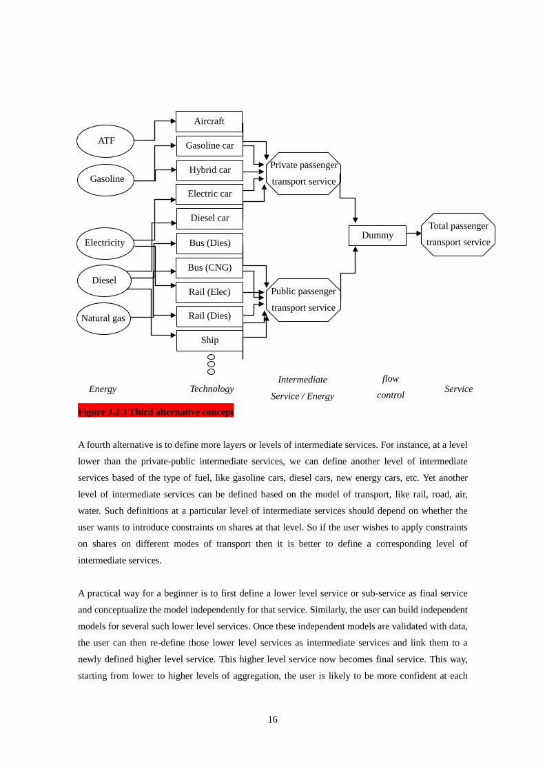
A third alternative is to define total passenger transport as final service demand (as in case of first

alternative), but also define disaggregated sub-services of second alternative as services. The latter

types of services are not final but ‘intermediate services’ as their levels are determined internally in

the model. Here technologies are defined specifically for, and compete to meet the demand of, an

intermediate service. Like in the first two alternatives, this competition within an intermediate

service can be restricted by bounds on technology shares. Although two technologies for different

intermediate services do not compete directly, their selection decisions may still be interlinked if

they consume the same fuel which may have limited availability. Moreover, the share of an

intermediate service (in the final service) can also be restricted by upper or lower bounds by defining

‘dummy’ or ‘flow control’ device that takes as input ‘intermediate energy’ corresponding to that

intermediate service and gives out the final service as output.

Public passenger

transport service

Gasoline car

Hybrid car

Diesel car

Bus (diesel)

Bus (CNG)


Electricity

Diesel

Natural gas


Rail (Electric)

Rail (Diesel)

Ship

Aircraft

ATF

Private passenger

transport service

16

Figure 3.2.3 Third alternative concept

A fourth alternative is to define more layers or levels of intermediate services. For instance, at a level

lower than the private-public intermediate services, we can define another level of intermediate

services based of the type of fuel, like gasoline cars, diesel cars, new energy cars, etc. Yet another

level of intermediate services can be defined based on the model of transport, like rail, road, air,

water. Such definitions at a particular level of intermediate services should depend on whether the

user wants to introduce constraints on shares at that level. So if the user wishes to apply constraints

on shares on different modes of transport then it is better to define a corresponding level of

intermediate services.

A practical way for a beginner is to first define a lower level service or sub-service as final service

and conceptualize the model independently for that service. Similarly, the user can build independent

models for several such lower level services. Once these independent models are validated with data,

the user can then re-define those lower level services as intermediate services and link them to a

newly defined higher level service. This higher level service now becomes final service. This way,

starting from lower to higher levels of aggregation, the user is likely to be more confident at each

Public passenger

transport service

Gasoline car

Hybrid car

Diesel car

Bus (Dies)

Bus (CNG)


Electricity

Diesel

Natural gas


Rail (Elec)

Rail (Dies)

Ship

Aircraft

ATF

Private passenger

transport service

Total passenger

transport service

Intermediate

Service / Energy

Dummy

flow

control

17

stage about the model’s database and baseline results.

STEP 2: Select model type, time horizon, unit of energy and price and data sheets in each

simulation case

In the worksheet “Cntl”, user can select model type, time horizon and units of price and energy.

User has two choices for Model Type – “FOR Enduse” and “FOR ACC”. “Enduse” is the regular

multi-period AIM/Enduse model which performs calculation of technology-mix and energy-mix for

every year within the selected time horizon, using a recursive dynamic optimization method. “ACC”

is the static version of AIM/Enduse model which performs calculation of Abatement Cost for a

single target (end) year alone.

Time horizon is represented by “START YEAR” (simulation start year) and “END YEAR”

(simulation end year). The start year must be the recent historical year for which reliable data are

available. End year is the year up to which the user wants to perform analysis.

“ENE UNIT” (unit of energy) is the unit in which all energy flows will be expressed. We suggest

“toe”. “PRICE UNIT” (unit of price) is the unit in which all costs will be expressed. We suggest

“1000US$”. User must be clear about the base year in which all input cost data are expressed.

Figure 3.2.4 Example of model type, time horizon, price unit, and energy unit (“Cntl”)

STEP 3: Select proper units for service demand, device unit

This is an important step. Before the user begins to enter data, he/she must decide what are the most

appropriate units for service demand and device unit. This choice must depend on the units in which

the data for service demand, specific service output of technologies and stock of technologies in the

start year are available to the user, and the kind of policies user wants to analyze.

For instance, suppose that the user has collected data of passenger transport services in start year in

number of vehicles, stock of vehicle-types in start year in number of vehicles and specific service

18

output of technologies (vehicle-types) in pkm/vehicle/year. Then the user has the following choices

of units:

(i) Service demand (pkm), Device unit (pkm): In this case the user will have to express

stock in start year in pkm by assuming average person-kilometers traveled in a

vehicle-type in a year. By making similar conversions the user will also have to express

projections of service demands in pkm. While making such projections the user must be

clear about the assumption of changing pkm per vehicle-type in the future years.

Specific service output in this case will be 1 (i.e. 1 pkm service per pkm device per

year). Specific energy input has to be expressed in average energy (toe) used per pkm

per year.

In this case the countermeasure of reduced travel by people can be analyzed by

reducing service demand (pkm). However it may be difficult to analyze together the

countermeasures of improving energy efficiency as well as utilization of vehicles. Both

these countermeasures will have to be reflected in reducing specific energy input. So it

might be better to analyze these two effects separately.

(ii) Service demand (pkm), Device unit (1 vehicle): In this case the user can enter stock in

start year directly in number of vehicle (of each vehicle-type). However, service

demand in start year as well as in future years will have to be expressed in pkm by

assuming average person-kilometers per vehicle in start year and future years. Specific

service output for a vehicle-type will be the average pkm per vehicle per year, i.e. the

assumption user made to estimate service demand in start year. Specific energy input

has to be expressed in average energy (toe) used per vehicle per year.


reducing service demand (pkm). The countermeasure of improving energy efficiency

can be analyzed by reducing specific energy input. The countermeasure of improving

utilization of vehicles can be analyzed by increasing specific service output. So effects

of all these countermeasures can be assessed independently as well as together.

(iii) Service demand (vehicles), Device unit (1 vehicle): In this case the user can enter stock

in start year directly in number of vehicles (of each vehicle-type). Service demand for

future years, for a vehicle-type, is also expressed in number of vehicles. While making

such projections the user must be clear about the assumption of average utilization of

vehicles in future years. Specific service output in this case will be 1 (i.e. 1 vehicle

service per vehicle device per year). Specific energy input has to be expressed in

average energy (toe) used per vehicle per year.


reducing specific energy input. The countermeasure of improving energy efficiency can

19

also be analyzed by reducing specific energy input. So it may be difficult to analyze the

two countermeasures – reduced travel and improved energy efficiency – together. The

countermeasure of improving utilization of vehicles can be analyzed by reducing

service demand (number of vehicles).

STEP 4: Collect and estimate essential data for start year

The user must collect and/or estimate the minimum essential data required to run the model

successfully for the start year. These are:

• Define region (sheet “Region”)

• Define sectors (sheet “Sector”)

• Define services in each sector and their units (sheet “Service”)

• Define energy types (sheet “Energy”)

• Define emission types (sheet “Gas”)

• Define technologies and enter for each technology its lifetime, Initial cost, O&M cost,

specific service output (for at least one service) and specific energy input (for at least one

energy type) (sheet “Device”)

• Stock of each technology in start year (sheet “Stock”)

• Service demand in start year (sheet “SRV_DM”)

• Emission factors of each energy type in start year (sheet “ENE_EMF”)

• Price of each energy type in start year (sheet “ENE_PRC”)

• Maximum and minimum shares of technologies in start year (sheet “SHR”)

• Define discount rate (sheet "RATE")

Note) If you define "intermediate services" or "maximum or minimum share of a certain technology

group", then you also need to set additional worksheet in the database interface, such as sheet "INT"

or sheet "OMMX" and so on. Please see Appendix in detail.

Figure 3.2.5 Example of region definition (“Region”)

20

Figure 3.2.6 Example of sector definition (“Sector”)

Figure 3.2.7 Example of energy definition and units (“Energy”)

Figure 3.2.8 Example of service definition and units (“Service”)

21

Figure 3.2.9 Example of emission definition and units (“Gas”)

Figure 3.2.10 Example of technology definition and data (“Device”)

Figure 3.2.11 Example of stock data of technology in start year (“Stock”)

22

Figure 3.2.12 Example of service demand data (“SRV_DM”)

Figure 3.2.13 Example of emission factor data (“ENE_EMF”)

Figure 3.2.14 Example of energy price data (“ENE_PRC”)

23

Figure 3.2.15 Example of service share data in baseline case (“SHR_BL”)

STEP 5: Run model and validate dataset for start year

Before running the model, the user must do the following validations checks on input data:

• Completeness check: All data listed in section 3.1.5 are entered.

• Consistency check: The service demand in start year and the stock of technologies in start

year are equivalent. If service demand and stock are expressed in the same unit (i.e. device

unit), then for each service the service demand must be equal to the sum of stocks of all

technologies providing that service in start year. If, for a service, service demand and stock

are expressed in different units then the equivalence can be checked by first converting

stocks in the unit of service demand and then verifying if the service demand is equal to the

sum of stocks of all technologies providing that service in start year.

The “enduse” model can be run for start year alone by selecting the same start year and end year in

sheet “Cntl”.

After running the model for start year, the user must do the following validation checks on output

results and verify if they are consistent with the collected/published data:

• Primary energy use – total, sector-wise, energy type-wise

• Final energy use – total, sector-wise, energy type-wise

• Emissions – gas-wise, sector-wise, energy type-wise

• Average energy intensity – sector-wise, service-wise (this can be calculated by dividing total

energy used in a sector or service by total service demand for that sector or service)

24

STEP 6: Estimate baseline data for future years

The user must estimate the minimum essential data required to run the model successfully for the

entire time horizon (start year to end year). These data are the same as mentioned in section 3.1.5,

except that additional estimates for future years need to be made for service demands and

maximum/minimum shares of technologies. In addition, if required as part of baseline, some other

data like emission factor and energy price too can be changed with time.

STEP 7: Run model and validate baseline data for future years

Validation of results for future years must be done for trends in certain aggregate indicators based on

the expert opinion of the user and others. These indicators can be the same as suggested for the start

year validation:

• Primary energy use – total, sector-wise, energy type-wise

• Final energy use – total, sector-wise, energy type-wise

• Emissions – gas-wise, sector-wise, energy type-wise

• Average energy intensity – sector-wise, service-wise (this can be calculated by dividing total

energy used in a sector or service by total service demand for that sector or service)

STEP 8: Construct scenarios for policy analysis

See examples in "APPENDIX IV. AIM/Enduse[Japan]" and " APPENDIX III. Exercise" as for how

to construct scenarios for policy analysis.

STEP 9: Run model and compare scenario results

See examples in "APPENDIX IV. AIM/Enduse[Japan]" and " APPENDIX III. Exercise" as for how

to compare scenario results.

25

APPENDIX I. Structure and Formulation of AIM/Enduse

I.1 Input & Output files of AIM/Enduse

I.1.1 Overview

1) Input files

・(case name).set ：AIM/Enduse GAMS set file

・(case name)_1.gms ：AIM/Enduse GAMS data file(1)

・(case name)_2.gms ：AIM/Enduse GAMS data file(2)

・(case name).inp ：AIM/Enduse case path file

・AIM_Enduse.BAT ：AIM/Enduse model executable file

・AIM_Enduse.err ：AIM/Enduse model error file

・AIM_MAC.bat ：AIM/Enduse[ACC] model executable file

・AIM_MAC.err ：AIM/Enduse[ACC] model error file

Note) Case name is arbitrarily specified by a user.

2) GAMS Program

・AIM_CMB.gms ：GAMS main program for AIM/Enduse model

・AIM_MAC.gms ：GAMS main program for AIM/Enduse[ACC]

・_interp.gms ：GAMS sub program for interpolation

・_errorout.gms ： (to be prepared)

・_emsfc.gms ：GAMS sub program for calculating emission factors

・_load_result.gms ： (to be prepared)

・_output.gms ：GAMS sub program for output

・aggregate.gms ： (to be prepared)

・_printout_old.gms ： (to be prepared)

・_printout_sp.gms ： (to be prepared)

・_printout.gms ： (to be prepared)

26

3) Output files

・(case name)_detail.csv ：Detailed Output file

・(case name)_cost.csv ：Output file related to cost per unit emission reduction

・(case name)_emsfc.csv ：Output file related to emission factors

・(case name)_internal.csv ：Output file related to internal service and energy balances

・(case name)_adjust.csv ：(to be prepared)

Note) Case name is arbitrarily specified by a user.

27

I.1.2 Input files of AIM/Enduse

1) AIM_Enduse.inp

-------------------------------------------------------------------------------------------------------- $SETGLOBAL INPUT C:¥Enduse_Global¥SAMPLE¥Enduse¥TRTFix --------------------------------------------------------------------------------------------------------

2) (Case name).set

Table I.1.1Element of indices in AIM/Enduse model

Code in AIM/Enduse model Description

I Region or LPS identifier

K Energy type

J Service type

L Technology

M Emission gas type

P *1 Removal technology

H Cohort type

YEAR(H) Simulation years

MR Region

M_MR(I,MR) Mapping among I and region MR

INT Internal service and energy pairs

JE_KE(INT,J,K) Mapping among internal service J and internal energy K (INT J K)

MR_INT(MR,INT) Mapping among region MR and internal service and energy pair INT (MR INT)

N Technology group share constraint

M_N(I,L,J,N) Mapping among technology group share constraint N, sector I, technology L and service J(I L J N)

MQ Emission constraint group (region and sector)

M_MQ(I,MQ) Target region and sector group for emission constraint (I MQ)

MG Emission constraint group (gas)

M_MG(M,MG) Target gas group for emission constraint (M MG)

ME Region and sector group for energy constraint

M_ME(I,ME) Mapping among I and ME (I ME)

NQ Observation sector of gas emission

N_MQ(I,NQ) Mapping among sector and region I and observation sector NQ

Note) *1 Comment only in AIM/Enduse interface.

28

3) (Case name)_1.gms

Table I.1.2 Exogenous Parameters in AIM/Enduse model


ACT_I(I) Flag of Activity (I)

AN_T(L,J,YV,Y) Service quantity per unit operation of recruited technology (L J YV Y)

EN_T(K,L,P,YV,Y) Energy consumption of recruited technology per unit operation (K L P YV Y)

SERV_T(I,J,YV,Y) Service amount required (I J YV Y)

GAS_T(I,K,M,YV,Y) CO2, SO2, NO2 Emission Factor (I K M YV Y)


Table I.1.3 Exogenous Parameters in AIM/Enduse model


V_YEAR(YEAR) Numeric of year

TAX_T(I,M,YV,Y) Emission tax prescribed (I M YV Y)

TAXE_T(I,K,YV,Y) Energy tax prescribed (I K YV Y)

ALPHA(I,L) Discount rate (I L)

TN(L) Life span of technology (L)

BN_T(I,L,P,YV,Y) Initial cost of the recruited technology (I L P YV Y)

F0_T(L,M,YV,Y) Gas generated per unit operation, independent with energy (L M YV Y)

G0_T(I,L,P,YV,Y) Operation Cost per unit operating excluding energy cost (I L P YV Y)

DN(L,P,M) *1 Pollutant removal ratio(L P M)

BX_T(L,P,P1) *1 Initial cost of exchanging(L,P,P1)

UB(K,L) Ratio of material use to total input (K L)

BETA(I,L) Shape parameter of survival rate function (I L)

A(I,L,J) Service quantity per unit operation of stock technology (I L J)

E(I,K,L,P) Energy consumption of stocked technology per unit operation (I K L P)

D(I,L,P,M) *1 Pollutant removal ratio of stocked technology (I L P M)

SC(I, L,P,H) Stock quantity (I L P H)

THMX_T(I,L,J,YV,Y) Maximum allowable service share (I L J YV Y)

THMN_T(I,L,J,YV,Y) Minimum allowable service share (I L J YV Y)

GE_T(I,K,YV,Y) Energy Price (I K YV Y)

OMMX_T(N,YV,Y) Maximum allowable service share of technology group(N YV Y)

OMMN_T(N,YV,Y) Minimum allowable service share of technology group(N YV Y)

QMAX_T(MQ,MG,YV,Y) Maximum allowable emission of Gas (MQ MG YV Y)

EMAX_T(ME,K,YV,Y) Maximum allowable energy supply (ME K YV Y)

EMIN_T(ME,K,YV,Y) Minimum allowable energy supply (ME K YV Y)

SGMX_T(I,J,YV,Y) Maximum allowable regional service share(I J YV Y)

29


SGMN_T(I,J,YV,Y) Minimum allowable regional service share(I J YV Y)

ROMX_T(I,L,YV,Y) Maximum allowable stock quantity(I L YV Y)

ROMN_T(I,L,YV,Y) Minimum allowable stock quantity(I L YV Y)

TUMX_T(I,L,YV,Y) Maximum allowable recruit quantity(I L YV Y)

TUMN_T(I,L,YV,Y) Minimum allowable recruit quantity(I L YV Y)

ETMX_T(I,L,YV,Y) Maximum allowable change rate of recruit quantity(I L YV Y)

ETMN_T(I,L,YV,Y) Minimum allowable change rate of recruit quantity(I L YV Y)

PHI_T(I,J,YV,Y) Social service improvement (I J YV Y)

GAM_T(I,L,YV,Y) Operating efficiency Loss (I L YV Y)

XI_T(I,L,YV,Y) Countermeasure for Energy efficiency change by maintenance (I L YV Y)

SCN_T(L,P,YV,Y) Subsidy rate for recruited technology (L P YV Y)

SCO_T(L,P,YV,Y) Subsidy rate for operation cost (L P YV Y)

SCX_T(L,P,P1,YV,Y) *1 Subsidy rate for exchange (L P P1 YV Y)

EQ(NQ,M) Observed gas emission in the base year(NQ M)

Note) *1 Comment only in AIM/Enduse interface.

30

I.1.3 Input files of AIM/Enduse[ACC]

1) AIM_MAC.inp

-------------------------------------------------------------------------------------------------------- $SETGLOBAL INPUT C:¥Enduse_Global¥SAMPLE¥ACC¥TRTFix --------------------------------------------------------------------------------------------------------

2) (Case name).set

Table I.1.4 Element of indices in AIM/Enduse[ACC]

Code in AIM/Enduse[ACC] model Description

I Sector and region

K Energy type

J Service type

M Emission gas type

L Technology

YEAR Simulation years

MR Region group

MRI(MR) International region

MRD(MR) Domestic region

M_MR(I,MR) Mapping among I and region MR

INT Internal service and energy pairs

JE_KE(INT,J,K) Mapping among internal service J and internal energy K (INT J K)

MR_INT(MR,INT) Mapping among MR and INT

N Technology group share constraint

M_N(I,L,J,N) Mapping among technology group share constraint

ME Energy constraint group

M_ME(I,ME) Mapping among I and Energy constraint group

NQ Observation sector of gas emission

M_NQ(I,NQ) Mapping among sector and region I and observation sector NQ (I NQ)

31


Table I.1.5 Exogenous Parameters in AIM/Enduse[ACC]


AN_T(L,J,YV,Y) Service quantity per unit operation of recruited technology

EN_T(K,L,YV,Y) Energy consumption of recruited technology per unit operation

F0_T(L,M,YV,Y) Gas generated per unit operation, independent with energy

GAS_T(I,K,M,YV,Y) Emission Factor (direct emission)

SERV_T(I,J,YV,Y) Service amount required


Table I.1.6 Exogenous Parameters in AIM/Enduse[ACC]


V_YEAR(YEAR) Numeric of simulation year

YEAR_T Target year

YEAR_B Base year

CP_T(I,YV,Y) Carbon price

ALPHA(I,L) Discount rate

TN(L) Life span of technology

BN_T(I, L,YV,Y) Initial cost of the recruited technology

G0_T(I,L,YV,Y) Operation Cost per unit operating excluding energy cost

UB(K,L) Ratio of material use to total input

THBMX_T(I,L,J,YV,Y) Maximum allowable service share in baseline case

THBMN_T(I,L,J,YV,Y) Minimum allowable service share in baseline case

THCMX_T(I,L,J,YV,Y) Maximum allowable service share in countermeasure case

THCMN_T(I,L,J,YV,Y) Minimum allowable service share in countermeasure case

GE_T(I,K,YV,Y) Energy Price

OMMX_T(N,YV,Y) Maximum allowable service share of technology group

OMMN_T(N,YV,Y) Minimum allowable service share of technology group

PHI_T(I,J,YV,Y) Social service improvement

GAM_T(I,L,YV,Y) Operating efficiency Loss

XI_T(I,L,YV,Y) Countermeasure for Energy efficiency change by maintenance

EMAX_T(ME,K,YV,Y) Maximum allowable energy supply

EMIN_T(ME,K,YV,Y) Minimum allowable energy supply

SGMX_T(I,J,YV,Y) Maximum allowable regional service share

SGMN_T(I,J,YV,Y) Minimum allowable regional service share

EQ(NQ,M) Observed gas emission in the start year

32

I.1.4 Output files of AIM/Enduse

1) (Case name)_detail.csv

Text written in (case name)_detail.csv is as follows. Text is mostly same but partially different

between two models. AIM/Enduse model has “RemPrcs”.

--------------------------------------------------------------------------------------------------------------

"Kind","Region","Item","Device","RmvPrcs","year","VALUE"

"DEV","TRT+JPN","_","TPPCOG_EXT2","NON","2005", 6.60453836213393E+07

--------------------------------------------------------------------------------------------------------------

Table I.1.7 AIM/Enduse Output

Code (Kind) (Item) Definition

Kind CST Item= RCA, RCI, MDA, MDI, MNT, TXE, TXM

DEV Operating quantity (I,L,Y)

EMS Emission quantity (I,M,L,Y)

ENG Energy consumption (I,K,L,Y)

SHR Service share (I,J,L,Y)

SRV Service supply (I,J,L,Y)

STK Stock quantity (I,L,Y)

RCT Recruited quantity (I,L,Y)

Region (Sector Type)+(Region) The sector code + the region code

Item Kind = CST RCA Total annualized investment cost(I,L,Y)

RCI Total initial investment cost(I,L,Y)

MDA Total annualized cost of exchanging removal process(I,L,Y)

MDI Total initial cost of exchanging removal process(I,L,Y)

MNT Total operating cost including energy cost, material cost, maintenance cost etc. (I,L,Y)

TXE Energy tax payment

TXM Emission tax payment

Kind = DEV - -

Kind = EMS (Gas Type) The gas code

Kind = ENG (Energy Type) The energy code

Kind = SHR (Service Type) The service code

Kind = SRV (Service Type) The service code

Kind = STK - -

Device (Energy Device) The device code

33

2) (Case name)_cost.csv

（to be prepared）

3) (Case name)_emscf.csv


4) (Case name)_internal.csv


5) (Case name)_adjust.csv


34

I.1.5 Output files of AIM/Enduse[ACC]

1) (Case name)_detail.csv

Text written in (case name)_detail.csv in AIM/Enduse[ACC] model is as follows. Text is mostly

same but partially different between two models. AIM/Enduse[ACC] model has “Carbon Price”.

--------------------------------------------------------------------------------------------------------------

“Kind”,”Region”,”Item”,”Device”,”YEAR”,”Value”,”Carbon Price”

"DEV","TRT+JPN","_"," TPPCOG_HEF2", “2020”,3.02585E+07,5.00E-01

--------------------------------------------------------------------------------------------------------------

Table I.1.8 AIM/Enduse[ACC] Output

Code (Kind) (Item) Definition

Kind CST Item= AC, RCA, RCI, MNT, TXM, DLC, DLCP

DEV Operating quantity (I,L,Y)

EMSD Direct emission quantity (I,M,L,Y)

EMSI Indirect emission quantity (I,M,L,Y)

ENG Energy consumption (I,K,L,Y)

RDC Total reduction (I,M,L,Y)

SHR Service share (I,J,L,Y)

SRV Service supply (I,J,L,Y)

Region (Sector Type)+(Region) The sector code + the region code

Item Kind = CST AC Cost per unit reduction (I,L,Y)

RCA Total annualized investment cost (I,L,Y)

RCI Total initial investment cost (I,L,Y)

MNT Total operating cost including energy cost, material cost, maintenance cost etc. (I,L,Y)

TXM Emission tax payment(I,L,Y)

DLC Total cost of emission reduction from baseline(I,L,Y) DLCP Total cost of emission reduction from baseline

excluding negative cost (I,L,Y) Kind = DEV - -

Kind = RDC (Gas Type) The gas code

Kind = EMSD (Gas Type) The gas code

Kind = EMSI (Gas Type) The gas code

Kind = ENG (Energy Type) The energy code

Kind = SHR (Service Type) The service code

Kind = SRV (Service Type) The service code

Kind = STK - -

Device (Energy Device) The device code

35

2) (Case name)_cost.csv


3) (Case name)_emscf.csv


4) (Case name)_internal.csv


5) (Case name)_adjust.csv


36

I.2 Theoretical formulation

I.2.1 Formulation of AIM/Enduse

1. Indices and sets

The suffix of indices and sets are defined as follows in the AIM-Enduse model

i : Sector and region

j : Service type

k : Energy type

l : Device or measure (i.e. mitigation option)

h : Device cohort

m : Gas (emission) type

p : Gas (emission) removal process

t : Simulation year

0t : Base year

jW : Set of combinations of device and removal process ( , )l p that can satisfy service type j

MQ : Group of sectors and regions i categorized for emission constraints MQY : Set of sectors and regions i belonging to the group MQ

MG : Group of gases m categorized for emission constraints

MGZ : Set of gases m belonging to the group MG

ME : Group of sectors and regions i categorized for energy supply constraints

MEY : Set of sectors and regions i belonging to the group ME

MR : Group of sectors and regions i categorized for internal energy balance constraints

INT : Group of combinations of internal energy and internal service ( , )k j

MRY : Set of sectors and regions i belonging to the group MR

INTJ : Set of services j belonging to the INTth internal service

INTK : Set of energy k belonging to the INTth internal energy

n : Number of share ratio constrains for group of devices l

nU : Set of devices l that is targeted in the nth group share ratio constrains

nG : Set of combinations of sectors/regions and service ( , )i j that is targeted in the nth group

share ratio constrains

NQR : Set of sectors and regions i′ belonging to the group NQ

37

iR : Group of NQ belonging to sectors and regions i

mGWP : Global warming potential of a gas m

2. Expression for emission quantity estimation

Emission quantity (CO2 equivalent) miQ of a gas m in a sector and region i is expressed by

Equation (1). Emission quantity miQ is calculated by multiplying operating quantity , ,l p iX by

emission quantity , ,ml p ie

of a gas m per unit operation of combination of a device l with removal

process p in a sector and region i and adding up quantity of emissions from all devices. Emission

quantity , ,ml p ie

of a gas m is composed of energy-related emissions and non-energy-related

emissions and expressed by Equation (2).

, , , ,( , )

j

m mi l p i l p i

j l p W

Q X e∈

= ⋅∑ ∑ EQ_EMISS(i,m) (1)

( ) ( ) ( ), , 0, , , , , , , , ,1 1 1m m m ml p i l k i l i k l p i k l l p i

k

e f f E U dξ

= + ⋅ − ⋅ ⋅ − ⋅ −

∑ EQ_EM(i,p,l,m) (2)

where miQ : Emission quantity of a gas m in a sector and region i (Note: CO2 equivalent)

, ,l p iX : Operating quantity of a combination of a device l with removal process p in a sector and

region i

, ,ml p ie : Emission quantity of a gas m per unit operation of combination of a device l with

removal process p in a sector and region i

0,mlf : Emission of a gas m from operations other than energy combustion of a unit of device l

(i.e. same as gas m’s emission coefficient of a device l )

,m

k if : Emission of a gas m from combustion of energy type k by a unit energy use of device

l in a sector and region i

,l iξ : Energy efficiency improvement ratio by device l in sector and region i , due to efficiency

improvement of operation and management

, , ,k l p iE : Energy consumption of energy type k per unit operation of a combination of a device l

with removal process p in a sector and region i (i.e. same as specific energy input to a

device)

,k lU : Proportion of energy type k used for non-combustion operations in a device l (i.e. used

as material process in a device l )

38

, ,ml p id : Removal ratio of gas m per unit operation of combination of a device l with removal

process p in a sector and region i .

3. Expression for energy consumption estimation

Consumption of energy type k in a sector and region i is estimated by adding up consumption of

energy k from all devices, expressed by Equation (3).

, , , , , , ,( , )

(1 )j

ek i l i k l p i l p i

j l p W

Q E Xξ∈

= − ⋅ ⋅∑ ∑ EQ_ENG(i,k) (3)

where

,ei kQ : Consumption of energy type k in a sector and region i

4. Constraint conditions

1) Emission constraints

Emission quantity of a gas m in a sector and region i must not exceed its allowable maximum

emission limit MGMQQ , in the case of setting emission constraints on the MG th group of gases m in

MQ th group of sectors and regions i , expressed by Equation (4).

, , , ,( , )MQ MG MQ MG j

m m MGi l p i l p i MQ

i Y m Z i Y m Z j l p W

Q X e Q∈ ∈ ∈ ∈ ∈

= ⋅ ≤

∑ ∑ ∑ ∑ ∑ ∑ EQ_GEC(MQ,MG) (4)

where MGMQQ : Allowable maximum limit on emissions of the MG th group of gases m in the MQ th

group of sectors and regions i

2) Energy supply constraints

Total quantity of supply of energy type k cannot exceed its allowable maximum energy supply

quantity max,ME kE or fall below its allowable minimum energy supply quantity min

,ME kE , in the case of

setting energy supply constraints on energy type k in the ME th group of sectors and regions i ,

expressed by Equation (5) and Equation (6) respectively.

max, , , , , , , ,

( , )(1 )

ME ME j

ek i l i k l p i l p i ME k

i Y i Y j l p WQ E X Eξ

∈ ∈ ∈

= − ⋅ ⋅ ≤

∑ ∑ ∑ ∑ EQ_ESCMAX(ME,k) (5)

39

min, , , , , , , ,

( , )(1 )

ME ME j

ek i l i k l p i l p i ME k

i Y i Y j l p WQ E X Eξ

∈ ∈ ∈

= − ⋅ ⋅ ≥

∑ ∑ ∑ ∑ EQ_ESCMIN(ME,k) (6)

where

max,ME kE : Allowable maximum supply quantity of energy type k in the ME th group of sectors and

regions i

min,ME kE : Allowable minimum supply quantity of energy type k in the ME th group of sectors and

regions i

3) Total operating capacity constraints

Total operating quantity , ,l p iX of a combination of a device l with removal process p in a sector

and region i must not exceed its operating quantity by stock , , ,l p h iS of a device l by operating

rate ,(1 )l i+ Λ , expressed by Equation (7).

( ), , , , , ,1l p i l i l p h ih

X S≤ + Λ ⋅∑ EQ_OCC(i,l,p) (7)

where

,l iΛ : Operating allowance rate (or negative value of unused rate) of a device l in a sector and

region i (Note: ,1 l i+ Λ is taken as operating rate device l and used as input in the

Enduse database interface)

, , ,l p h iS : Stock of a combination of the h th device cohort of a device l with removal process p in

a sector and region i

4) Total service demand-and-supply balance constraints

For a given final service demand quantity ,j iD of service j in a sector and region i , its demand

must not exceed the total service demand by multiplying the quantity of total service output supplied

by all devices by service supply rate ,1 j i+ Ψ , expressed by Equation (8)

( ), , , , , ,( , )

1j

j i j i l j i l p il p W

D A X∈

≤ + Ψ ⋅ ⋅∑ EQ_SVC(i,j) (8)

where

, ,l j iA : Supply output of service j per unit operation of a device l in a sector and region i (i.e.

same as specific service output from a device)

40

,j iΨ : Service efficiency improvement rate of service j in sector and region i (Note: Negative

of ,j iΨ is the loss incurred during delivery of service j , for example transmission and

distribution loss of electricity supply. ,1 j i+ Ψ , service supply rate, is used as input in the


,j iD : Total service demand quantity of service j in a sector and region i

5) Internal energy and internal service balance constraints

In the case of accommodating internal energy with internal service in the MR th group of sectors

and regions i , for its group of combinations of internal energy and internal service ( ),j k that is

classified in INT th group, the demand ,ei kQ of internal energy k must not exceed the supply ,j iD

of internal service j , expressed by Equation (9). For example, secondary energy consumed in final

energy consumption sectors must be met by energy produced in energy conversion sectors.

( )

, ,

, , , , , , , , , , ,( , ) ( , )

1 (1 )

MR INT MR INT

MR INT j MR INT j

ej i k i

i Y j J i Y k K

j i l j i l p i l i k l p i l p ii Y j J l p W i Y k K j l p W

D Q

A X E Xξ

∈ ∈ ∈ ∈

∈ ∈ ∈ ∈ ∈ ∈

≥

∴ + Ψ ⋅ ≥ − ⋅ ⋅

∑ ∑ ∑ ∑

∑ ∑ ∑ ∑ ∑ ∑ ∑

EQ_END(MR,INT) (9)

6) Device share ratio constraints on service output

In the case of setting device share constraints on service output j by a device l in a sector and

region i , share ratio of service output of its device l to the total service output of all devices

regarding service j must not exceed the maximum limit max, ,l j iθ or fall below the minimum limit

min, ,l j iθ , expressed by Equation (10) and Equation (11) respectively.

,

max, , , , , , , , , ,

( , ) i j

l j i l j i l p i l j i l p il p W p

A X A Xθ ′ ′ ′′ ′ ∈

⋅ ⋅ ≥ ⋅∑ ∑ EQ_SRCMX(i,j,l) (10)

,

min, , , , , , , , , ,

( , ) i j

l j i l j i l p i l j i l p il p W p

A X A Xθ ′ ′ ′′ ′ ∈

⋅ ⋅ ≤ ⋅∑ ∑ EQ_SRCMN(i,j,l) (11)

where max, ,l j iθ : Maximum share rate of service j of a device l to the total service output of all devices in

a sector and region i min, ,l j iθ : Minimum share rate of service j of a device l to the total service output of all devices in


41

7) Share ratio constraints on service output for group of devices

In the case of setting share rate constraints on service output j by a group of devices U in a

sector and region i , share ratio of service output of its group of devices to the total service output of

all devices regarding service j must not exceed the maximum limit maxnω or fall below the

minimum limit minnω , expressed by Equation (12) and Equation (13) respectively.

( )

max, , , , , , , ,

( , ) ', ' ( , )n j n n

n l j i l p i l j i l p ii j G l p W i j G l U p

A X A Xω ′ ′ ′∈ ∈ ∈ ∈

⋅ ⋅ ≥ ⋅

∑ ∑ ∑ ∑ ∑ EQ_SGCMX(n) (12)

( )

min, , , , , , , ,

( , ) ', ' ( , )n j n n

n l j i l p i l j i l p ii j G l p W i j G l U p

A X A Xω ′ ′ ′∈ ∈ ∈ ∈

⋅ ⋅ ≤ ⋅

∑ ∑ ∑ ∑ ∑ EQ_SGCMN(n)

(13)

where maxnω : Maximum share rate of service j of group of devices in the nth constraint to the total

service output of all devices in a sector and region i minnω : Minimum share rate of service j of group of devices in the nth constraint to the total

service output of all devices in a sector and region i

8) Share ratio constraints on service output in sector and region i

For a given service supply j , share ratio of service j in a sector and region i to the total service

in all sectors and regions can be considered by the following constraints. For example in coal mining,

the ratio of coal production in a certain region to the world coal production is constrained by these

equations. These equations are applicable only to multi-regional model. Share ratio of service output

j in a sector and region i to the total service in all sectors and regions must not exceed the

maximum limit max,j iσ or fall below the minimum limit min

,j iσ , expressed by Equation (14) and

Equation (15) respectively.

( ) ( )max, , ' , , ' , , ' , , , , ,

' ( , ) ( , )

1 1j j

j i j i l j i l p i j i l j i l p ii l p W l p W

A X A Xσ∈ ∈

+ Ψ ⋅ ⋅ ≥ + Ψ ⋅ ⋅

∑ ∑ ∑

EQ_SWCMX(i,j) (14)

42

( ) ( )min, , ' , , ' , , ' , , , , ,

' ( , ) ( , )

1 1j j

j i j i l j i l p i j i l j i l p ii l p W l p W

A X A Xσ∈ ∈

+ Ψ ⋅ ⋅ ≤ + Ψ ⋅ ⋅

∑ ∑ ∑

EQ_SWCMX(i,j) (15)

where max,j iσ : Maximum share rate of service j in a sector and region i to the total service in all

sectors and regions min,j iσ : Minimum share rate of service j in a sector and region i to the total service in all sectors

and regions

9) Device recruitment quantity constraints

Quantity of a device l recruited in the current year must not exceed the maximum value max,l iτ or

fall below the minimum value min,l iτ , expressed by Equation (16) and Equation (17) respectively.

max

, , ,l p i l ip

r τ≤∑ EQ_RTCMX(i,l) (16)

min, , ,l p i l i

pr τ≥∑ EQ_RTCMN(i,l) (17)

where

, ,l p ir : Recruitment quantity of a device l with removal process p in a sector and region i

max,l iτ : Maximum recruitment quantity of a device l in a sector and region i

min,l iτ : Minimum recruitment quantity of a device l in a sector and region i

10) Annual growth rate constraints on device recruitment quantity

Annual growth rate of recruitment quantity of a device l from the previous year must not exceed

the maximum annual growth ratio max,l iη or fall below the minimum annual growth ratio min

,l iη ,


( )max, , , , ,1l p i l i l p i

p pr rη≤ + ⋅∑ ∑ EQ_DRCMX(i,l) (18)

( )min, , , , ,1l p i l i l p i

p pr rη≥ + ⋅∑ ∑ EQ_DRCMN(i,l) (19)

where

, ,l p ir : Recruitment quantity of a device l with removal process p in the previous year in a

43

sector and region i

max,l iη : Maximum annual growth ratio of recruitment quantity of a device l from the previous

year in a sector and region i

min,l iη : Minimum annual growth ratio of recruitment quantity of a device l from the previous year

in a sector and region i

11) Device stock quantity constraints

Stock quantity of a device l must not exceed the maximum value max,l iρ or fall below the

minimum value min,l iρ , expressed by Equation (20) and Equation (21) respectively.

max

, , , ,l p h i l ih p

S ρ≤∑∑ EQ_STCMX(i,l) (20)

min, , , ,l p h i l i

h pS ρ≥∑∑ EQ_STCMN(i,l) (21)

where

max,l iρ : the maximum value of stock quantity of device l in sector and region i

min,l iρ : the maximum value of stock quantity of device l in sector and region i

5. Stock quantity balance

1) Existing stock quantity

Every device l has a lifetime and its device l is retired and recruited over time. Stock quantity of

combination of a device l and removal process p in the current year is calculated by Equation

(22). The first term of right-hand side represents the quantity of remaining stock from the previous

year after considering retirement due to its life time. The second term represents additional quantity

of combination of a device l with removal process p in a sector and region i recruited in the

current year. The third term denotes the net stock of other combinations of a device l that are

exchanged by its combination with removal process p in the current year. The last term represents

the quantity of retired devices regardless of its life time.

( )1 11

, , , , , , , ,, , , , , , , , ,l p h i l p i l p h il p h i l p p h i l p p h ip

r wS SS M M→ →+ −= + −∑ EQ_SCS(i,l,p,h) (22)

The first parameter in the right-hand member in Equation (22) represents remained amount from the

previous year considering the lifetime of a device l , expressed by Equation (23). ,l hSR represents

44

the remaining ratio.

, , , ,, , , l p h i l hl p h iSS S SR= ⋅

(23)

The remaining ratio ,l hSR from the previous year is defined as follows; firstly, assuming a function

that represents relations between remaining ratio and elapsed years t since a device l installation,

and differentiating that function. Weibull distribution function is defined as a remaining ratio

function in this study, expressed by Equation (24). (Note: in the previous version of the AIM/Enduse

model, an inverse of lifetime of device l is considered as a remaining ratio).

( ) expl

ll

ttT

fβ

β

−

= (24)

Equation (25) is calculated by differentiating Equation (24) with respect to year t

( )( ) ( )

( )1 1

expl ll

l l l

l l

l l l

t td tt tdt T T T

f fβ ββ

β β ββ β− − ⋅ ⋅

⋅ − = ⋅

= − − (25)

Thus, considering the cohort year hAGE of the h th device cohort of a device l (i.e. the elapsed

years since the h th device cohort of a device l is introduced), the remaining ratio ,l hSR of the h th

device cohort of a device l from the previous year is expressed by Equation (26) ( )1

, 1l

l

l hl h

l

AGET

SRβ

ββ −⋅

= − (26)

where




a sector and region i in the previous year

, , ,l p h iSS :Remaining ratio of the h th device cohort of a device l with removal process p in a

sector and region i from the previous year

, ,l p ir : Additional quantity of combination of a device l with removal process p in a sector and

region i recruited in the current year

1, , ,l p p h iM →:Stock of a combination of the h th device cohort of a device l with removal process p in

a sector and region i in the previous year that is replaced in the current year by its

combination with another removal process 1p

1, , ,l p p h iM →:Stock of a combination of the h th device cohort of a device l with removal process 1p

in a sector and region i in the previous year that is replaced in the current year by its

combination with another removal process p

45

, , ,l p h iw : Quantity of combination of a device l with the removal equipment p retired regardless

of its life time

,l hSR : Remaining ratio of the h th device cohort of a device l from the previous year

lβ : Parameter of weibull distribution function of s device l

lT : Life of device l

hAGE : the cohort year of the h th device cohort of device l (i.e. the elapsed years since the h th

device cohort of a device l is introduced)

2) Stock exchange constraints on existing stock

Stock of a device l recruited in a given year will retire according its life time. Stock of a

combination of the h th device cohort of a device l with removal process p in a sector and region

i in the previous year can be replaced (or exchanged) in the current year by its combination with

another removal process 1p . However, the stock that is replaced in the current year cannot exceed

the remaining stock of a device l that is passed on from the previous year.

1

1

, , , , , ,l p h i l p p h ip

SS M →≥∑ EQ_SEC(i,l,p,h) (27)

3) Additional quantity to the stock in the current year

Quantity of combination of a device l with removal process p in a sector and region i recruited

in the current year is added to the stock as a new cohort number of device l

, ,' ', , ,l p t i l p iS r= (28)

where

' 't : cohort number of a device l recruited in the year t

4) Performance change of stock device

The performance of a device l can also change over time. Average performance of combination of

a device l with removal process p on a given parameter in the current year is estimated from the

weighted average of performances of its stock passed on from the previous year, its quantity

recruited in the current year, and the net stock of this combination that is obtained from exchanges

with other combinations of a device l in the current year. Expressions (29), (30) and (31) estimate

46

the average performance of combination of a device l with removal process p on different

performance-parameters. Change in average performance of combination of a device l with removal

process p over time can be calculated by repeatedly calculating expressions (29), (30) and (31) in

every year.

Performance change of emission ratio

1

11

, , , , , ,, , , , , , , , , ,1

, , , , , , ,

l p h i l p h im ml p i l p h i l p i l p p h i

h h p

m

l p i l p i l p p h ih p

SS wd S d M

d r M

→

→

−

⋅ = ⋅ −

+ ⋅ +

∑ ∑ ∑

∑∑

PRR_EQ(i,l,p,m) (29)

Performance change of energy efficiency

( )

1

1

1 1 1

1

, , , , , ,, , , , , , , , , , , ,

, , , , , , , , , , , , ,

l p h i l p h ik l p i l p h i k l p i l p p h ih h p

Ek l p i l p i k l p i k l p p l p p h i

p h

SS wE S E M

E r E M

→

→ →

− ⋅ = ⋅ −

+ ⋅ + + ∆ ⋅

∑ ∑ ∑

∑ ∑

EER_EQ(i,k,l,p) (30)

Performance change of service efficiency

( ), , , , , , , ,, , , , , , , , ,l p h i l p h i l j il j i l p h i l j i l p ih p h p p

SS wA S A A r−⋅ = ⋅ + ⋅∑∑ ∑∑ ∑

SER_EQ(i,l,j) (31)

where

, ,ml p id : Removal ratio of a gas m from combination of a device l with removal process p in a

sector and region i

, ,ml p id

: Removal ratio of a gas m from combination of a device l with removal process p in a

sector and region i in the previous year

, ,

m

l p id

: Removal ratio of a gas m from combination of a device l with removal process p in a

sector and region i , for stock of that combination obtained in the current year from either

recruitment or exchange with other combinations

, , ,k l p iE : Energy consumption of energy kind k per unit operation of combination of a device l

with removal process p in a sector and region i

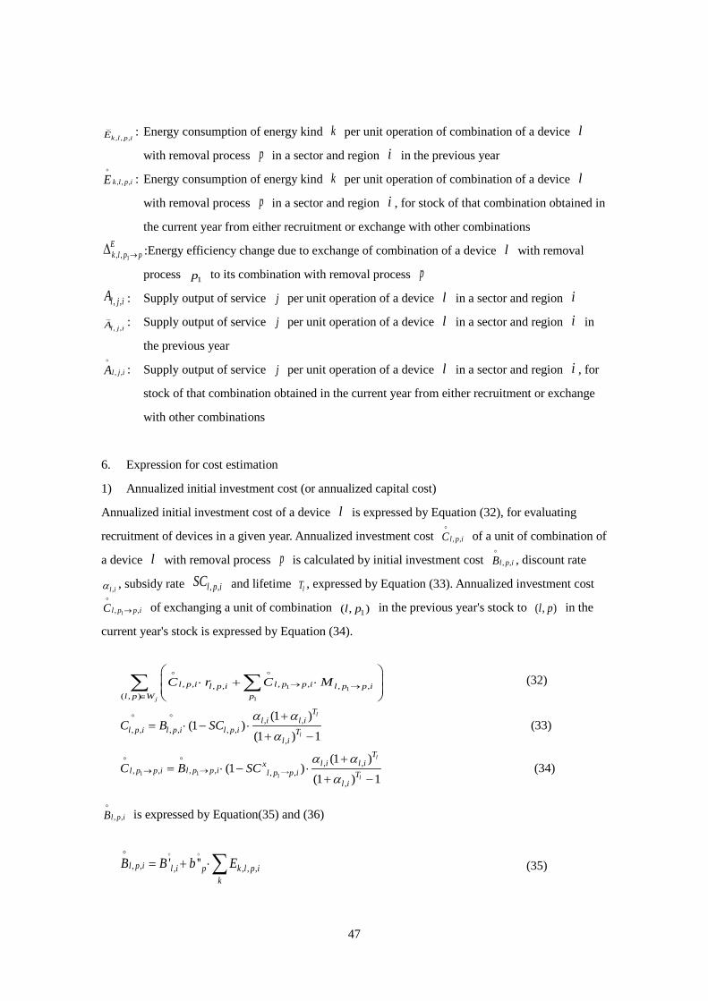
47

, , ,k l p iE : Energy consumption of energy kind k per unit operation of combination of a device l

with removal process p in a sector and region i in the previous year

iplkE ,,,

: Energy consumption of energy kind k per unit operation of combination of a device l

with removal process p in a sector and region i , for stock of that combination obtained in

the current year from either recruitment or exchange with other combinations E

pplk →∆1,, :Energy efficiency change due to exchange of combination of a device l with removal

process 1p to its combination with removal process p

, ,l j iA : Supply output of service j per unit operation of a device l in a sector and region i

, ,l j iA : Supply output of service j per unit operation of a device l in a sector and region i in

the previous year

ijlA ,,

: Supply output of service j per unit operation of a device l in a sector and region i , for

stock of that combination obtained in the current year from either recruitment or exchange

with other combinations

6. Expression for cost estimation

1) Annualized initial investment cost (or annualized capital cost)

Annualized initial investment cost of a device l is expressed by Equation (32), for evaluating

recruitment of devices in a given year. Annualized investment cost , ,l p iC

of a unit of combination of

a device l with removal process p is calculated by initial investment cost , ,l p iB

, discount rate

,l iα , subsidy rate , ,l p iSC and lifetime lT , expressed by Equation (33). Annualized investment cost

1, ,l p p iC →

of exchanging a unit of combination 1( , )l p in the previous year's stock to ( , )l p in the

current year's stock is expressed by Equation (34).

1 1

1

, , , ,, , , ,( , ) j

l p i l p p il p i l p p il p W p

C r C M→ →∈

⋅ + ⋅

∑ ∑

(32)

, ,, , , , , ,

,

(1 )(1 )

(1 ) 1

l

l

Tl i l i

l p i l p i l p i Tl i

C B SCα α

α

+= ⋅ − ⋅

+ −

(33)

11 1

, ,, ,, , , ,

,

(1 )(1 )

(1 ) 1

l

l

Tl i l ix

l p p il p p i l p p i Tl i

C B SCα α

α→→

+= ⋅ − ⋅

+ −

→ (34)

, ,l p iB

is expressed by Equation(35) and (36)

, , , , , ,' ''l p i l i p k l p ik

B B b E= + ⋅∑ 。。

(35)

48

( ), , , , ,1k l p i p k l iE e E′= + ⋅ (36)

where

, ,l p iC

: Annualized investment cost of a unit of combination of a device l with removal process

p in a sector and region i

1, ,l p p iC →

:Annualized investment cost of exchanging a unit of combination 1( , )l p in the previous

year's stock to ( , )l p in the current year's stock in sector and region i

, ,l p iB

: Initial investment cost of recruiting one unit of combination of a device l with removal

process p in a sector and region i

,l iα : Discount rate for investment (Note: corresponding to internal rate of return or hurdle rate)

, ,l p iSC : Subsidy rate for recruitment of a device l with removal process p in a sector and region

i

1, ,l p p iB →

: Initial investment cost of exchanging a unit of combination 1( , )l p to in the previous year's

stock to ( , )l p in the current year's stock in a sector and region i

1, ,l p p iSC → :Subsidy rate for exchanging a unit of combination 1( , )l p to in the previous year's stock

to ( , )l p in the current year's stock in a sector and region i

,l iB′

: Initial investment cost of recruiting one unit of energy a device l in a sector and region i

pb′′

: Initial investment cost of removal process p per energy consumption of combination of a

device l with removal process p

, ,k l iE′ : Energy consumption of energy kind k per unit operation of energy a device l in a sector

and region i

pe : Additional energy consumption rate of removal process p

2) Annual running cost

Annualized running cost of a device l is expressed by Equation (37), considering cost of energy

used and cost of operation and management of its device. Annualized running cost of a unit of

combination of a device l with removal process p is calculated by operating cost (non-energy

cost) 0, ,l p ig , energy cost ,k ig , subsidy rate , ,

rl p iSC .

( ) ( )0, , , , , , , , , , ,

( , )

1- 1i

rl p i k i l i k l p i l p i l p i

l p W k

g g E SC Xξ∈

+ ⋅ ⋅ ⋅ − ⋅

∑ ∑ (37)

0, ,l p ig is expressed by Equation (38)

49

0 0 0, , , , , ,l p i l i p k l p i

k

g g g E′ ′′= + ⋅∑

(38)

where 0, ,l p ig : Operating cost (non-energy cost) per unit operation of combination of a device l with


,k ig : Energy cost of energy kind k per unit operation of combination of a device l with


, ,rl p iSC : Subsidy rate for operating cost of additional quantity of combination of a device l with

removal process p in a sector and region i 0,l ig ′ : Operating cost (non-energy cost) per unit operation of energy a device l in a sector and

region i 0pg ′′ : Operating cost per unit operation of removal process p per energy consumption of

combination of a device l with removal process p

7. Objective function

Objective function is the total cost in a given year as shown in Equation (39). The total cost

comprises total annualized initial investment cost (only for recruitments in that year), total running

cost, total cost of emission tax and total cost of energy tax in that year. Decisions for recruitment

quantity and operational quantity for all feasible combinations of devices and removal processes in a

given year are made based on the criterion of total cost minimization.

1 1

1

, , , ,, , , ,( , ) j

xl p i l p p il p i l p p i

i l p W p

TC C r C M→ →∈

= ⋅ + ⋅ ∑ ∑ ∑

( ) ( )0, , , , , , , , , , ,1- 1 r

l p i k i l i k l p i l p i l p ik

g g E SC Xξ + + ⋅ ⋅ ⋅ − ⋅

∑

, , minm m e ei i k i k i

m kQ Qε ε + ⋅ + ⋅ →

∑ ∑ (39)

where

TC : Total cost miε : Emission tax on gas m in a sector and region i

,ek iε : Energy tax on energy k in a sector and region i

50

8. Base year emission calibration of gas m

If there are any reported or measured emission amounts of a gas m in a sector and region i in

the base year, it is necessary to adjusting the calculated parameters in the model to the reported or

measured emission values. Adjustment factor (i.e. calibration coefficient) mNQρ

is represented by

Equation (40), when reported emission 0,mNQEQ

of a gas m in set of sectors and regions i belonging to the group NQ . (for example, if NQ is defined as Japan, 0,m

NQEQ represents the total

"reported" emissions of a gas m in the base year, 0,

NQ

mi

i RQ ′

′∈∑

represents the total "calculated"

emissions of a gas m in the base year in the model)

0,

0,NQ

mi

i RmNQ m

NQ

Q

EQρ

′′∈

=∑

EQ_RO(NQ,m) (40)

where


In the result, calibrated emissions ,adj miQ in the base year are expressed by Equation (41). iR

represents the group NQ belonging to sectors and regions i , NQR represent a set of sectors and

regions i′ belonging to the group NQ .

,

''

i

NQ

madj m m ii NQ m

iNQ Ri R

QQQ

ρ∈

∈

= ⋅∑ ∑

EQ_QX(i,m) (41)

where 0,mNQEQ : the total reported emissions of a gas m in the base year in set of sectors and regions i

belonging to the group NQ 0,miEQ : the total calculated emissions of a gas m in a sector and region i in the base year in the

model ,adj m

iQ : adjusted emissions of a gas m in a sector and region i mNQρ : Adding adjustment factor for a gas m belonging to the group NQ

51

I.2.2 Formulation of AIM/Enduse[ACC]

1. Indices and set

The suffix of indices and sets are defined as follows in the AIM/Enduse[ACC] tool.

i : Sector and region

j : Service type

k : Energy type

l : Device or measure (i.e. mitigation option)

m : Gas (emission) type

t : Simulation year

0t : Base year

jW : Group of devices l that can satisfy service type j

ME : Group of sectors and regions i categorized for energy supply constraints

MEY : Set of sectors and regions i belonging to the group ME

MR : Group of sectors and regions i categorized for internal energy balance constraints

INT : Group of combinations of internal energy and internal service ( , )k j

MRY : Set of sectors and regions i belonging to the group MR

INTJ : Set of services j belonging to the INTth internal service

INTK : Set of energy k belonging to the INTth internal energy

n : Number of share ratio constrains for group of devices l

nU : Set of devices l that is targeted in the nth group share ratio constrains

nG : Set of combinations of sectors/regions and service ( , )i j that is targeted in the nth group

share ratio constrains

lV : Group of services j that can be provided by a device l

H : Set of devices l′ that provide the same service output j as the device l in a sector and

region i and that incremental service output ,l iD ′∆ of device l′ from the baseline is

larger than zero.


iR : Group of NQ belonging to sectors and regions i

mGWP : Global warming potential of a gas m

52

2. Expression for emission quantity estimation

Emission quantity (CO2 equivalent) miQ of a gas m in a sector and region i is expressed by

Equation (1). Emission quantity miQ is calculated by multiplying operating quantity ,l iX by

emission quantity ,ml ie

of a gas m per unit operation of a device l in a sector and region i and

adding up quantity of emissions from all devices. Emission quantity ,ml ie

of a gas m is composed

of energy-related emissions and non-energy-related emissions and expressed by Equation (2).

, ,m mi l i l i

l

Q X e= ⋅∑ EQ_EMISS(i,m) (1)

( ) ( ), 0, , , , ,1 1m m ml i l k i l i k l k l

k

e f f E Uξ= + ⋅ − ⋅ ⋅ −∑ EQ_EM(i,l,m) (2)

Emission quantity (hereinafter, indirect emissions) miQA , after allocating emissions caused by

electricity, heat or steam from the energy supply side to the energy demand side, is expressed by

Equation (3). Emission quantity ,ml iea is the indirect emission of a gas m per unit operation of a

device l in a sector and region i. Emission quantity ,ml iea

of gas m is composed of

non-energy-related emissions 0,mlf and energy-related indirect emissions ,

mk ifa of a gas m from

combustion of energy type k by a unit energy use of a device l in a sector and region i , and

expressed by Equation (4).

, ,m mi l i l i

l

QA X ea= ⋅∑ EQ_EMISSA(i,m) (3)

( ) ( ), 0, , , , ,1 1m m ml i l k i l i k l k l

k

ea f fa E Uξ= + ⋅ − ⋅ ⋅ −∑ EQ_EMA(i,l,m) (4)

where miQ : Emission quantity of a gas m in a sector and region i (Note: CO2 equivalent)

miQA : Indirect emission quantity of a gas m in a sector and region i (Note: CO2 equivalent)

,l iX : Operating quantity of a device l in a sector and region i

,ml ie : Emission quantity of a gas m per unit operation of a device l in a sector and region i

,ml iea : Indirect emission quantity of a gas m per unit operation of a device l in a sector and

region i

0,mlf : Emission of a gas m from operations other than energy combustion of a unit of device l

(i.e. same as gas m’s emission coefficient of a device l )

,m

k if : Emission of a gas m from combustion of energy type k by a unit energy use of device

53

l in a sector and region i (Internal energies such as electricity, heat or steam are set at

the value of zero)

,mk ifa : Indirect emission of a gas m from combustion of energy type k by a unit energy use of

device l in a sector and region i (Internal energies such as electricity, heat or steam are

set at the values after allocating from the energy supply side to the energy demand side.

Energy consumption for producing internal energy is set at the value of zero.)

,l iξ : Energy efficiency improvement ratio by a device l in a sector and region i , due to

efficiency improvement of operation and management of a device l .

,k lE : Energy consumption of energy type k per unit operation of a device l (i.e. same as

specific energy input to a device)

,k lU : Proportion of energy type k used for non-combustion operations in a device l (i.e. used

as material process in a device l )

3. Expression for energy consumption estimation

Consumption of energy type k in a sector and region i is estimated by adding up consumption of

energy k from all devices, expressed by Equation (5).

, , , ,(1 )ei k l i k l l i

l

Q E Xξ= − ⋅ ⋅∑ EQ_ENG(i,k) (5)

where

,ei kQ : Consumption of energy type k in a sector and region i

4. Constraint conditions

1) Energy supply constraints

Total quantity of supply of energy type k cannot exceed its allowable maximum energy supply

quantity max,ME kE or fall below its allowable minimum energy supply quantity min

,ME kE , in the case of

setting energy supply constraints on energy type k in the ME th group of sectors and regions i ,


( ) max, , , , ,1

ME ME

ei k l i k l l i ME k

i Y i Y lQ E X Eξ

∈ ∈

= − ⋅ ⋅ ≤

∑ ∑ ∑ EQ_ESCMAX(ME,k) (6)

54

( ) min, , , , ,1

ME ME

ei k l i k l l i ME k

i Y i Y lQ E X Eξ

∈ ∈

= − ⋅ ⋅ ≥

∑ ∑ ∑ EQ_ESCMIN(ME,k) (7)

where

max,ME kE : Allowable maximum supply quantity of energy type k in the ME th group of sectors and

regions i

min,ME kE : Allowable minimum supply quantity of energy type k in the ME th group of sectors and

regions i

2) Total operating capacity constraints

Total operating quantity ,l iX of a device l in a sector and region i must not exceed its

operating quantity by stock ,l iS of a device l by operating rate ,(1 )l i+ Λ , expressed by Equation

(8).

( ), , ,1l i l i l iX S= + Λ ⋅ EQ_OCC(i,l) (8)

where

,l iΛ : Operating allowance rate (or negative value of unused rate) of a device l in a sector and

region i (Note: ,1 l i+ Λ is taken as operating rate a device l and used as input in the


,l iS : Stock of a device l in a sector and region i

3) Total service demand-and-supply balance constraints

For a given final service demand quantity ,j iD of service j in a sector and region i , its demand

must be equal to the total service demand by multiplying the quantity of total service output supplied

by all devices by service supply rate ,1 j i+ Ψ , expressed by Equation (9)

( ), , , .1j

j i j i l j l il W

D A X∈

= + Ψ ⋅ ⋅∑ EQ_SDC(i,j) (9)

where

,l jA : Supply output of service j per unit operation of a device l in a sector and region i (i.e.

same as specific service output from a device)

55

,j iΨ : Service efficiency improvement rate of service j in a sector and region i (Note:

Negative of ,j iΨ is the loss incurred during delivery of service j , for example

transmission and distribution loss of electricity supply. ,1 j i+ Ψ , service supply rate, is used

as input in the Enduse database interface)

,j iD : Total service demand quantity of service j in a sector and region i

4) Internal energy and internal service balance constraints

In the case of accommodating internal energy with internal service in the MR th group of sectors and

regions i , for its group of combinations of internal service and internal energy ( ),j k that is

classified in the INT th group, the demand ,ei kQ of internal energy k must be equal to the supply

,j iD of internal service j , expressed by Equation (10). For example, secondary energy consumed in

final energy consumption sectors must be met by energy produced in energy conversion sectors.

( )

, ,

, , , , , ,1 (1 )

MR INT MR INT

MR INT j MR INT

ej i k i

i Y j J i Y k K

j i l j l i l i k l l ii Y j J l W i Y k K l

D Q

A X E Xξ

∈ ∈ ∈ ∈

∈ ∈ ∈ ∈ ∈

=

∴ + Ψ ⋅ = − ⋅ ⋅

∑ ∑ ∑ ∑

∑ ∑ ∑ ∑ ∑ ∑ 　

EQ_END(MR,INT) (10)

5) Device share ratio constraints on service output

In the case of setting device share constraints on service output j by a device l in a sector and

region i , share ratio of service output of its device l to the total service output of all devices

regarding service j must not exceed the maximum limit max, ,l j iθ or fall below the minimum limit

min, ,l j iθ , expressed by Equation (11) and Equation (12) respectively.

max, , ', , '. , ,

' j

l j i l j i l i l j l il W

A X A Xθ∈

⋅ ⋅ ≥ ⋅∑ EQ_SRCMX(i,j,l) (11)

min, , ', , '. , ,

' j

l j i l j i l i l j l il W

A X A Xθ∈

⋅ ⋅ ≤ ⋅∑ EQ_SRCMN(i,j,l) (12)

where max, ,l j iθ : Maximum share rate of service j of a device l to the total service output of all devices in

a sector and region i min, ,l j iθ : Minimum share rate of service j of a device l to the total service output of all devices in


56

6) Share ratio constraints on service output for group of devices

In the case of setting share rate constraints on service output j by a group of devices U in a

sector and region i , share ratio of service output of its group of devices to the total service output of

all devices regarding service j must not exceed the maximum limit maxnω or fall below the

minimum limit minnω , expressed by Equation (13) and Equation (14) respectively.

max', '. , ,

( , ) ' ( , )n j n n

n l j l i l j l ii j G l W i j G l U

A X A Xω∈ ∈ ∈ ∈

⋅ ⋅ ≥ ⋅

∑ ∑ ∑ ∑ EQ_SGCMX(n) (13)

min', '. , ,

( , ) ' ( , )n j n n

n l j l i l j l ii j G l W i j G l U

A X A Xω∈ ∈ ∈ ∈

⋅ ⋅ ≤ ⋅

∑ ∑ ∑ ∑ EQ_SGCMN(n) (14)

where maxnω : Maximum share rate of service j of a group of devices in the nth constraint to the total

service output of all devices in a sector and region i minnω : Minimum share rate of service j of a group of devices in the nth constraint to the total

service output of all devices in a sector and region i

7) Share ratio constraints on service output in sector and region i

For a given service supply j , share ratio of service j in a sector and region i to the total service

in all sectors and regions can be considered by the following constraints. For example in coal mining,

the ratio of coal production in a certain region to the world coal production is constrained by these

equations. These equations are applicable only to multi-regional model. Share ratio of service output

j in a sector and region i to the total service in all sectors and regions must not exceed the

maximum limit max,j iσ or fall below the minimum limit min

,j iσ , expressed by Equation (15) and

Equation (16) respectively.

( ) ( )max, , ' , . ' , , .

'

1 1j j

j i j i l j l i j i l j l ii l W l W

A X A Xσ∈ ∈

+ Ψ ⋅ ⋅ ≥ + Ψ ⋅ ⋅

∑ ∑ ∑ EQ_SWCMX(i,j) (15)

( ) ( )min, , ' , . ' , , .

'

1 1j j

j i j i l j l i j i l j l ii l W l W

A X A Xσ∈ ∈

+ Ψ ⋅ ⋅ ≤ + Ψ ⋅ ⋅

∑ ∑ ∑ EQ_SWCMX(i,j) (16)

57

where max,j iσ : Maximum share rate of service j in a sector and region i to the total service in all

sectors and regions min,j iσ : Minimum share rate of service j in a sector and region i to the total service in all sectors

and regions

5. Stock quantity balance

Stock ,l iS of a device l in a sector and region i in the simulation year t is calculated by

adding the remained stock in the simulation year t of its device l that existed in the base year 0t

and recruitment quantity ,l ir of its device l in a sector and region i in the simulation year t

and deducing quantity ,l iw of device l retired regardless of its life time in a sector and region i .

( )0

0, , , ,

l

t tT

l i l i l i l iS S e r w−

−= ⋅ + − EQ_SCS(i,l) (17)

where 0,l iS : Stock of a device l in a sector and region i in the base year 0t

,l ir : Recruitment quantity of a device l in a sector and region i

,l iw : Quantity of a device l retired regardless of its life time in a sector and region i

lT : Life of device l

6. Expression for incremental cost estimation

1) Annualized initial investment cost (or annualized capital cost)

Annualized initial investment cost of a device l is expressed by Equation (18). Annualized

investment cost ,l iC of its device l is calculated by initial investment cost ,l iB , discount rate ,l iα ,

and lifetime lT , expressed by Equation (18).

, ,, ,

,

(1 )(1 ) 1

l

l

Tl i l i

l i l i Tl i

C Bα α

α

+= ⋅

+ − EQ_CN(i,l) (18)

where

,l iC : Annualized investment cost of a device l in a sector and region i

,l iB : Initial investment cost of recruiting one unit of a device l in a sector and region i

,l iα : Discount rate for investment (Note: corresponding to internal rate of return or hurdle rate)

58

2) Annual running cost

Annualized running cost of a device l is expressed by Equation (19), considering cost of energy

used and cost of operation and management of its device. Annualized running cost of a device l is

calculated by operating cost (non-energy cost) 0,l ig and energy cost ,k ig .

( )0, , , , ,1l i k i l i k l l i

k

g g E Xξ + ⋅ ⋅ ⋅

∑ － (19)

where 0,l ig : Operating cost (non-energy cost) per unit operation of a device l in a sector and region i

,k ig : Energy cost of energy kind k per unit operation of a device l in a sector and region i

3) Total annualized cost per unit operation of a device l

The annualized cost ,l iCM per unit operation of a device l in a sector and region i , including

the fixed cost, energy cost , and maintenance cost, is expressed by Equation (20).

( ) ( )0, , , , , , ,1 1l i l i l i k i l i k l l i

k

CM C g g Eξ = + + ⋅ ⋅ ⋅ + Λ

∑ － EQ_CM(i,l) (20)

where

,l iCM : The total annualized cost per unit operation of a device l in a sector and region i

4) Annualized cost per unit service output j

The annualized cost ,l iCS per unit service output j of a device l in a sector and region i is

expressed by Equation (21).

( ) ( ),

,, , ,1 1

l il i

l j j i l ij

CMCS

A=

⋅ + Ψ ⋅ + Λ∑ EQ_CS(i,l) (21)

where

,l iCS : The annualized cost per unit service output j of a device l in a sector and region i

5) Annualized cost per unit service output j in the baseline

The annualized cost ,refj iCS per unit service output j in a sector and region i in the baseline is

estimated by dividing the sum of annualized cost per unit service output j of all devices by the sum

59

of service output j of all devices, expressed by Equation (22). , ,refl j iθ represents the share of

service output j of each device l in a sector and region i in the baseline.

, , ,ref ref, , , ,

, .

j

j

j

l j l i l il W

j i l j i l il j l i l W

l W

A X CS

CS CSA X

θ∈

∈∈

⋅ ⋅

= = ⋅⋅

∑∑∑

EQ_CSRF(i,j) (22)

where

,refj iCS : The annualized cost per unit service output j in a sector and region i in the baseline

, ,refl j iθ : The share of service output j of each device l in a sector and region i in the baseline

6) Incremental annualized cost per unit service output j of a device l

The incremental annualized cost ,l iCS∆ per unit service output j of a device l in a sector and

region i is expressed by Equation (23). lV represents the group of service j that can be

provided by a device l .

ref, , ,

l

l i l i j ij V

CS CS CS∈

∆ = −∑ EQ_DLUC(i,l) (23)

where

,l iCS∆ : annualized cost per unit service output j of a device l in a sector and region i

7. Expression for additional GHG emissions reductions estimation

1) Emissions of a gas m per unit service output j

Emission quantity (CO2 equivalent) ,ml iQS of a gas m per unit service output j of a device l in

a sector and region i is expressed by Equation (24). ,mk ifb represents indirect emissions of gas

m from combustion of energy type k by a unit energy use of a device l in a sector and region

i .

( ) ( )

( ) ( )0, , , , ,

,, , ,

1 1

1 1

m ml k i l i k l k l

m kl i

l j j i l ij

f fb E UQS

A

ξ+ ⋅ − ⋅ ⋅ −=

⋅ + Ψ ⋅ + Λ

∑∑

EQ_QS(i,l,m) (24)

where

,ml iQS ：Emission quantity (CO2 equivalent) of a gas m per unit service output j of a device l in

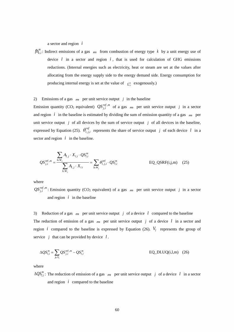
60


,mk ifb : Indirect emissions of a gas m from combustion of energy type k by a unit energy use of

device l in a sector and region i , that is used for calculation of GHG emissions

reductions. (Internal energies such as electricity, heat or steam are set at the values after

allocating from the energy supply side to the energy demand side. Energy consumption for

producing internal energy is set at the value of ,m

k if exogenously.)

2) Emissions of a gas m per unit service output j in the baseline

Emission quantity (CO2 equivalent) ,,

ref mj iQS of a gas m per unit service output j in a sector

and region i in the baseline is estimated by dividing the sum of emission quantity of a gas m per

unit service output j of all devices by the sum of service output j of all devices in the baseline,

expressed by Equation (25). , ,refl j iθ represents the share of service output j of each device l in a

sector and region i in the baseline.

, , ,ref , ref, , , ,

, .

j

j

j

ml j l i l i

l Wm mj i l j i l i

l j l i l Wl W

A X QS

QS QSA X

θ∈

∈∈

⋅ ⋅

= = ⋅⋅

∑∑∑

EQ_QSRF(i,j,m) (25)

where ,

,ref mj iQS : Emission quantity (CO2 equivalent) of a gas m per unit service output j in a sector

and region i in the baseline

3) Reduction of a gas m per unit service output j of a device l compared to the baseline

The reduction of emission of a gas m per unit service output j of a device l in a sector and

region i compared to the baseline is expressed by Equation (26). lV represents the group of

service j that can be provided by device l .

ref ,, , ,

l

m m ml i j i l i

j V

QS QS QS∈

∆ = −∑ EQ_DLUQ(i,l,m) (26)

where

,ml iQS∆ : The reduction of emission of a gas m per unit service output j of a device l in a sector

and region i compared to the baseline

61

8. Expression for abatement costs and GHG emissions reduction potentials estimation

1) Abatement cost per unit reduction of GHG emissions from the baseline

The abatement cost ,l iAC per unit reduction of GHG emissions by a device l in a sector and

region i compared to the baseline is estimated from the incremental annualized cost ,l iCS∆ per

unit service output j of a device l divided by the emissions reductions of all GHGs ,GHGl iQS∆ per

unit service output j of a device l , in a sector and region i compared to the baseline.

, ,,

, ,

l i l il i GHG m

l i l im

CS CSAC

QS QS∆ ∆

= =∆ ∆∑

EQ_AC(i,l) (27)

where

,GHGl iQS∆ : Emissions reductions of all GHGs per unit service output j of a device l in a sector

and region i compared to the baseline

,l iAC : The abatement cost per unit reduction of GHG emissions by a device l in a sector and

region i compared to the baseline

2) Device implementation quantity constraints

If the abatement cost ,l iAC per unit reduction of GHG emissions by a certain device l in a sector

and region i compared to the baseline is larger than the emission tax (carbon tax) miε set

exogenously by a user, its device l should not be implemented as mitigation options. Thus, the

service output j of its device l must not exceed the service output j of its device l in the

baseline, expressed by Equation (28).

( ) ( )ref, , . , , , , .

,

1 1j

j i l j l i l j i j i l j l il W

ml i i

A X A X

where AC

θ

ε

∈

+ Ψ ⋅ ⋅ ≤ ⋅ + Ψ ⋅ ⋅

>

∑ EQ_TIC(I,L,J) (28)

miε : Emission tax (CO2 equivalent) of gas m in a sector and region i

3) Incremental service output from the baseline

If the abatement cost ,l iAC per unit reduction of GHG emissions by a certain device l in a sector

and region i compared to the baseline is smaller than the emission tax (carbon tax) miε set

exogenously by a user, incremental amount ,l iD∆ of service output j of its device l from the

baseline is expressed by Equation (29).

62

( ) ( )ref, , , . , , , , .1 1

j

l i j i l j l i l j i j i l j l ij l W

D A X A Xθ∈

∆ = + Ψ ⋅ ⋅ − ⋅ + Ψ ⋅ ⋅

∑ ∑ EQ_DLD(I,L) (29)

where

,l iD∆ : Incremental service output j of a device l in a sector and region i from the baseline

4) Emissions reduction potentials of a gas m compared to the baseline

Emissions reduction potentials ,ml iQ∆ of a gas m in a sector and region i by introducing a

device l , whose abatement cost ,l iAC per unit reduction of GHG emissions compared to the

baseline is smaller than the emission tax (carbon tax) miε set exogenously by a user, is expressed by

Equation (30). H represents the set of devices l′ that provide the same service output j as the

device l in a sector and region i and that incremental service output ,l iD ′∆ of a device l′ from

the baseline is larger than zero.

, ,, , ', ', ,

', ', ','

,

0

0 0

ml i l im m

l i l i l i l i l imm l i l i l Hl il H

l i

QS DQS D QS D where D

QS DQ

where D

∉∈

∆ ⋅ ∆∆ ⋅ ∆ + ⋅ ∆ ⋅ ∆ ∆ ≥ ∆ ⋅ ∆∆ =

∆ <

∑∑

EQ_DLQ(i,l,m) (30)

where

,ml iQ∆ : Emissions reduction potentials of a gas m of a device l in a sector and region i from

the baseline

9. Objective function Objective function is the total cost in a given year as shown in Equation (31). The total cost

comprises total annualized initial investment cost (only for recruitments in that year), total running

cost and total cost of emission tax in that year. Decisions for recruitment quantity and operational

quantity for all feasible devices in a given year are made based on the criterion of total cost

minimization.

( )0, , , , , , , ,1 minm m

l i l i l i k i l i k l i l i i ii l k m

TC C r g g E X Qξ ε = ⋅ + + ⋅ − ⋅ ⋅ + ⋅ →

∑ ∑ ∑ ∑

EQ_TC (31)

63

where

TC : Total cost miε : Emission tax on a gas m in a sector and region i

10. Base year emission calibration of a gas m

If there are any reported or measured emission amounts of a gas m in a sector and region i in

the base year, it is necessary to adjusting the calculated parameters in the model to the reported or

measured emission values. Adjustment factor (i.e. calibration coefficient) mNQρ

is represented by

Equation (32), when reported emission 0,mNQEQ

of a gas m in set of sectors and regions i belonging to the group NQ . (for example, if NQ is defined as Japan, 0,m

NQEQ represents the total

"reported" emissions of a gas m in the base year, 0,

NQ

mi

i RQ ′

′∈∑

represents the total "calculated"

emissions of a gas m in the base year in the model)

0,

0,NQ

mi

i RmNQ m

NQ

Q

EQρ

′′∈

=∑

EQ_RO(NQ,m) (32)

where


In the result, calibrated emissions ,adj miQ in the base year are expressed by Equation (33). iR

represents the group NQ belonging to sectors and regions i , NQR represent a set of sectors and

regions i′ belonging to the group NQ .

,

''

i

NQ

madj m m ii NQ m

iNQ Ri R

QQQ

ρ∈

∈

= ⋅∑ ∑

EQ_QX(i,m) (33)

where 0,mNQEQ : The total reported emissions of a gas m in the base year in set of sectors and regions i

belonging to the group NQ 0,miEQ : The total calculated emissions of a gas m in a sector and region i in the base year in the

model ,adj m

iQ : Adjusted emissions of a gas m in a sector and region i mNQρ : Adding adjustment factor for a gas m belonging to the group NQ

64

APPENDIX II. Description of interface of AIM/Enduse

II.1 Description of “(file name)_IN.xlsb”

II.1.1 Overview

“(File name)_IN.xlsb” is the input data user interface for AIM/Enduse model. Microsoft Excel2007

is desirable for the operating environment (note: the user whose operating environment is Windows

2003 should use “(file_name)_IN.xls” in “Excel2003”).

“(File name)_IN.xlsb” consists of main sheet named “Cntl”, and various other sheets.

The process of use of “(file name)_IN.xlsb” is as follows:

1) Open “(file name)_IN.xlsb” (note: any file name and file location can be selected by a user. e.g.

SAMPLE_IN.xlsb, BASE_IN.xlsb, SCENARIO1_IN.xlsb, etc.).

2) Enter the data in a “Cntl” sheet, “EMS_TAX” sheet, “ENE_TAX” sheet (Enduse Only), “RATE”

sheet and other data sheets (note: any name for the data sheets can be selected by a user). It is

mandatory to enter data in the sheets whose tab is colored in blue.

3) After finished entering the data, please click on “CREATE GAMS DATASET” in the “Cntl”

sheet, corresponding to either Enduse or ACC version that is selected to be run. If execution is

successful a message “Complete Creating GAMS Dataset” will be displayed, and the input data

set for GAMS program would be created in the folder which is specified by a user in column

“FILE DIRECTORY’ of the sheet “Cntl” in “(file name)_IN.xlsb”.

II.1.2 Rules for codes

The columns in “(file name)_IN.xlsb” which are marked '◆' are mandatory field to be entered by the

user. All the data entered in these columns are used for calculation by the model. Of these, there are

some columns that require the user to enter codes, for example, codes for case, region, sector, service,

energy, gas, device, etc. These codes must begin with a letter (A to Z, a to z) or digit (0 to 9) and

followed by letters, digits or limited characters such as '-' (minus) or '_' (underscore) only. Be careful

not to use '+' (plus),' ' (blank), '{}' (brace) etc for codes. If so, you cannot run the model and face

with errors. The length of a code is limited to maximum 63 letters. Examples of correct and incorrect

codes are:

Correct entry: TRT TRT1 trt_1

Incorrect entry: [TRT] TRT 1 {trt_1}

65

If you do not follow this rule, GAMS will stop running. The listing file that results from running the

model (“AIM_CMB.lst” for AIM/Enduse model and “AIM_MAC.lst” for AIM/Enduse[ACC]

model) contains the following error message because of an invalid code for example:

131 [TRT]+JPN "Transport in Japan"

**** $508 $609

353 M_MR("[TRT]+JPN","JPN")=1;

**** $170

**** LINE 231 INCLUDE C:¥Enduse_Global¥SAMPLE¥Enduse¥TRTFix.set

**** LINE 106 INPUT C:¥Enduse_Global¥SAMPLE¥Src¥AIM_CMB.gms

141 Symbol neither initialized nor assigned

A wild shot: You may have spurious commas in the explanatory

text of a declaration. Check symbol reference list.

170 Domain violation for element

172 Element is redefined

257 Solve statement not checked because of previous errors

300 Remaining errors not printed for this line

508 Blank needed between element and text

(-or- illegal character in element)

609 Embedded values need $onembedded

**** 49725 ERROR(S) 0 WARNING(S)

Table II.1.1 Rules for codes used in “(file name)_IN.xlsb”

Codes in columns marked '◆' Codes in columns without '◆' (not used in the calculation)

Number of Characters 63 63 Must begin with A letter or number Any character Permitted special character

-(minus), _(underscore), Any

The outline of the data sheet in “(file name)_IN.xlsb” is explained in the following section.

66

II.1.3 Control Sheet

The “Cntl” sheet as shown in Figure II.1.1 appears on opening “(file name)_IN.xlsb”

(e.g.SAMPLE_IN.xlsb). User has to specify basic information such as simulation start year,

simulation end year, energy unit, price unit, and whether error check is desired. The units set in the

“Cntl” sheet should be used as standard units in other sheets.

Table II.1.2 Items in the “Cntl” sheet

Items Format Comments

ERROR CHECK Two choices Select “do check” or “skip check” from a pull-down

menu. It is recommended to select “do check”, and then

the software automatically checks errors of input data in

each sheet.

START YEAR Integer Simulation start year.

END YEAR Integer Simulation end year.

ENE UNIT Character Energy unit used in the calculation.

PRICE UNIT Character Price unit used in the calculation.

In the “Cntl” sheet, user has to specify scenarios and parameters for each simulation case. “FOR

Enduse” means for AIM/Enduse user and “FOR ACC” means for AIM/Enduse[ACC] user.

First, user decides case name of each simulation case and enters it in the column titled “CASE

NAME”. Next, user selects simulation scenarios of emission tax, energy tax and discount rate by

entering appropriate data in the sheets with green tab named “EMS_TAX”, “ENE_TAX” and “RATE”

(note: user can’t change the sheet names of “EMS_TAX”, “ENE_TAX” and “RATE”).

As regards the remaining sheets, starting from “Region” to “EQ”, user select one of data sheets from

the sheets tab color is blue (note: sheet name tab color is blue can be arbitrarily set by a user).

In “SAMPLE_IN.xlsb”, a series of data sheets are already prepared, so user can use these for a

simulation. If needed, user can duplicate the original file, modify and use it for another simulation.

67

Figure II.1.1 Screen of the “Cntl” sheet

68

II.1.4 Sheets for Simulation Case

1) EMS_TAX: Emission tax pattern

A user can set various levels of emission tax (carbon price) as countermeasure cases. The

“EMS_TAX” sheet as shown in Figure II.1.2 specifies emission tax (carbon price) projections with

different emission tax codes specified in the “Cntl” sheet.

Table II.1.3 Items in the “EMS_TAX” sheet Columns Format Comments

CK *(asterisk) If you leave a blank, the given setting is considered in calculation. If you wish to exclude a row from calculation, check *(asterisk) for that row.

NO Integer Number of the sets. It is an independent number and is not used in the calculation.

CODE* Character Code of each emission tax projection for the region/sector. NAME Character Name of the tax code. It is not used in calculation. GAS** Character Gas code listed in “GAS” sheet or “ALL”. “ALL” means

all gases listed in the “GAS” sheet. REGION* Character Region code listed in “Region” sheet or “ALL”. “ALL”

means all regions listed in the “Region” sheet. SECTOR* Character Sector code listed in “Sector” sheet or “ALL”. “ALL”

means all sectors listed in the “Sector” sheet. EMISSION TAX* Single Emission tax for the region/sector. The monetary unit of an

emission tax should be the same as described in the “Cntl” sheet. User can set multi-year data in AIM/Enduse model calculation. In AIM/Enduse[ACC] model calculation, program reads only the value in the extreme left column, when user does not set muti-year data.

* Required field for all users. ** Required field for the Enduse users.

Figure II.1.2 Screen of the “EMS_TAX” sheet

69

A user can set various levels of energy tax as countermeasure cases. The sheet “ENE_TAX” shown

in Figure II.1.3 specifies tax projections with different energy tax codes as specified in the “Cntl”

sheet.

Table II.1.4 Items in the “ENE_TAX” sheet

Columns Format Comments

CK *(asterisk) If you leave a blank, the given setting is considered in

calculation. If you wish to exclude a row from calculation,

check *(asterisk) for that row.

NO Integer Number of the sets. It is an independent number and is not

used in the calculation.

CODE** Character Code of energy tax pattern for the region/sector. .

NAME Character Name of energy tax code. It is not used in calculation.

ENERGY** Character Energy code listed in “Energy” sheet or “ALL”. “ALL”

means all energy types listed in the “Energy” sheet.

REGION** Character Region code listed in “Region” sheet or “ALL”. “ALL”

means all regions listed in the “Region” sheet.

SECTOR** Character Sector code listed in“Sector” sheet or “ALL”. “ALL”

means all sectors listed in the “Sector” sheet.

ENERGY TAX** Single Energy tax for the region/sector for AIM/Enduse model.

The monetary unit should be the same as listed in the

“Cntl” sheet.

** Required field for the Enduse users.

Figure II.1.3 Screen of the “ENE_TAX” sheet

70

2) RATE: Discount rate pattern

The “Rate” sheet shown in Figure II.1.4 specifies the discount rate used in a scenario. This pattern is

used in the “File” sheet. Discount rate is used for the economic criteria of technology selection

considering the lifetime of technology options.

Table II.1.5 Items in the “RATE” sheet






used in calculation.

CODE* Character Code for discount rate for region/sector/device.

NAME Character Description of the code for discount rate.

REGION* Character Select a region code listed in “Region” sheet or “ALL”.

ALL means all regions listed in the “Region” sheet.

SECTOR* Character Select a sector code listed in “Sector” sheet or “ALL”.

ALL means all sectors listed in the “Sector” sheet.

DEVICE* Character Select a device code listed in “Device” sheet or “ALL”.

“ALL” means all devices listed in the “Device” sheet.

DISCOUNT RATE (%) Decimal, % Setting of discount rate for region/sector/device. The unit

of the discount rate is percent (%).

* Required field for all users.

Figure II.1.4 Screen of the “RATE” sheet

71

II.1.5 Sheets for Classification

1) Region: Region classification

The “Region” sheet as shown in Figure II.1.5 specifies regional classification. The regional code is

quoted in the “Device” sheet, “SRV_DMD” sheet, “ENE_EMF” sheet, “ENE_PRC” sheet and some

other sheets.

Table II.1.6 Items in the “Region” sheet







CODE* Character Every region code must be unique. “ALL” can not be used

as a code.

NAME Character Region name. It is not used in calculation.


Figure II.1.5 Screen of the “Region” sheet Note) Sheet name can be selected by the user.

72

2) Sector: Sector classification

The “Sector” sheet as shown in Figure II.1.6 specifies sector classification. Emissions by each sector

are calculated based on this classification. The sector code is quoted in the “Service” sheet, “Device”

sheet, “SHR” sheet, “SRV_DM” sheet, “ENE_EMF” sheet, “ENE_PRC” sheet and several other

sheets.

Table II.1.7 Items in the “Sector” sheet







CODE* Character Every sector code must be unique. “ALL” can not be used

as a code.

NAME Character Sector name. It is not used in calculation.


Figure II.1.6 Screen of the “Sector“ sheet Note) Sheet name can be selected by the user.

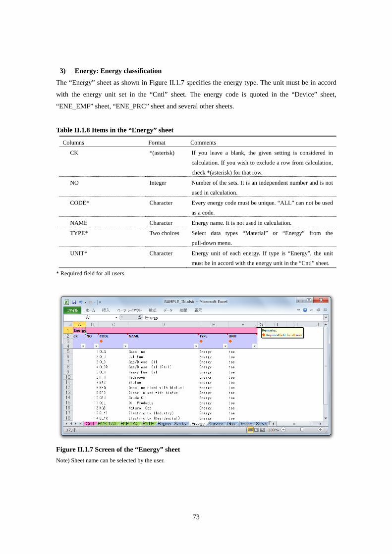
73

3) Energy: Energy classification

The “Energy” sheet as shown in Figure II.1.7 specifies the energy type. The unit must be in accord

with the energy unit set in the “Cntl” sheet. The energy code is quoted in the “Device” sheet,

“ENE_EMF” sheet, “ENE_PRC” sheet and several other sheets.

Table II.1.8 Items in the “Energy” sheet







CODE* Character Every energy code must be unique. “ALL” can not be used

as a code.

NAME Character Energy name. It is not used in calculation.

TYPE* Two choices Select data types “Material” or “Energy” from the

pull-down menu.

UNIT* Character Energy unit of each energy. If type is “Energy”, the unit

must be in accord with the energy unit in the “Cntl” sheet.


Figure II.1.7 Screen of the “Energy” sheet Note) Sheet name can be selected by the user.

74

4) Service: Service classification

The “Service” sheet as shown in Figure II.1.8 specifies the service type. A “service” refers to a

measurable demand in an enduse sector which can be met by one or more devices. The service code

is quoted in the “Device” sheet, “SHR” sheet, “SRV_DM” sheet and several other sheets.

Table II.1.9 Items in the “Service” sheet







CODE* Character Every service code must be unique in the list. “ALL” can

not be used as a code.

NAME Character Service name. It is not used in calculation.

SECTOR* Character Corresponding sector (from the “Sector sheet) to which the

service belongs.

UNIT* Character Service unit of each service.


Figure II.1.8 Screen of the “Service” sheet Note) Sheet name can be selected by the user.

75

5) Gas: Gas classification

The “Gas” sheet as shown in Figure II.1.9 specifies the gas type. The gas code is quoted in the

“Device” sheet, “ENE_EMF” sheet and several other sheets.

If a user wants to evaluate impacts of different greenhouse gases in terms of CO2 equivalent

(CO2eq), global warming potential (GWP) factors should be specified as emission coefficient of

each gas in the “ENE_EMF” sheet.

Table II.1.10 Items in the “Gas” sheet







CODE* Character Every gas code must be unique. “ALL” can not be used as a

code.

NAME Character Gas name. It is not used in calculation.

UNIT* Character Gas unit in terms of weight of either each specific gas or CO2

equivalent (CO2eq).


Figure II.1.9 Screen of the “Gas” sheet Note) Sheet name can be selected by the user.

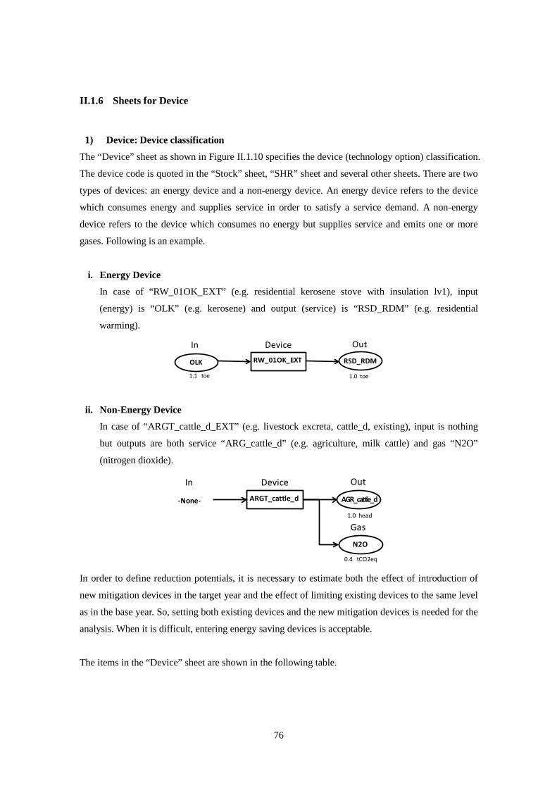
76

II.1.6 Sheets for Device

1) Device: Device classification

The “Device” sheet as shown in Figure II.1.10 specifies the device (technology option) classification.

The device code is quoted in the “Stock” sheet, “SHR” sheet and several other sheets. There are two

types of devices: an energy device and a non-energy device. An energy device refers to the device

which consumes energy and supplies service in order to satisfy a service demand. A non-energy

device refers to the device which consumes no energy but supplies service and emits one or more

gases. Following is an example.

i. Energy Device

In case of “RW_01OK_EXT” (e.g. residential kerosene stove with insulation lv1), input

(energy) is “OLK” (e.g. kerosene) and output (service) is “RSD_RDM” (e.g. residential

warming).

ii. Non-Energy Device

In case of “ARGT_cattle_d_EXT” (e.g. livestock excreta, cattle_d, existing), input is nothing

but outputs are both service “ARG_cattle_d” (e.g. agriculture, milk cattle) and gas “N2O”

(nitrogen dioxide).

In order to define reduction potentials, it is necessary to estimate both the effect of introduction of

new mitigation devices in the target year and the effect of limiting existing devices to the same level

as in the base year. So, setting both existing devices and the new mitigation devices is needed for the

analysis. When it is difficult, entering energy saving devices is acceptable.

The items in the “Device” sheet are shown in the following table.

RW_01OK_EXT

In Out

1.1 toe 1.0 toe

RSD_RDMOLK

Device

ARGT_cattle_d

In Out

0.4 tCO2eq

1.0 head

AGR_cattle_d

N2O

Device

-None-

Gas

77

Table II.1.11 Items in the “Device” sheet

Columns Format Comments CK *(asterisk) If you leave a blank, the given setting is considered in calculation.

If you wish to exclude a row from calculation, check *(asterisk) for that row.

NO Integer Number of the data sets. It is an independent number and is not used in calculation.

CODE* Character Technology code. Every code must be unique. “ALL” can not be used as a code.

NAME Character Technology name. It is not used in calculation. LIFE TIME* Single(>0) Life time of the technology. SHAPE PMT.** Single(>0) Numerical parameter of a parametric family of probability

distributions. INITIAL COST* Single(≧0) Initial capital investment cost per device unit. The monetary unit

should be the same as listed in the “Cntl” sheet. O&M COST* Single(≧0) Operations & maintenance cost per unit of operation. The

monetary unit should be the same as listed in the “Cntl” sheet. SECTOR Character Corresponding sector for the service listed in the “Sector” sheet. OUT - - Maximum allowable number of service outputs that can be

defined for a device is four. CODE* Character Output service code. The code should be listed in the “Service”

sheet. UNIT Character Corresponding unit of the service listed in the "Service" sheet.

QNT.* Single Service quantity output per unit operation of the technology. IN - - Maximum allowable number of energy and other inputs that can

be defined for a device is eight. CODE* Character Input energy code. The code should be listed in the “Energy”

sheet. UNIT Character Corresponding unit of the energy/material listed in the “Energy”

sheet. QNT.* Single Energy/material consumed by the technology per unit operation. N.E. Single Usage ratio of energy or material input for non-energy use (e.g.

non fuel combustion use) such as making raw product. If you set the rate as 100%, it means that all use is for non-energy purpose and there is no energy or material input for fuel combustion, thus no GHG will be emitted.

GAS - - Maximum allowable number of gases that can be defined for a device is four.

CODE* Character Gas emission code. The code should be listed in the “Gas” sheet. UNIT Character Corresponding unit of the gas listed in the “Gas” sheet. QNT.* Single Gas emitted per unit operation of device, excluding the energy or

combustion related emission. ALT.NAME & NOTE Character Explanation of the value. Remarks for calculation basis, and

calculation process. It is not used in calculation. FILE Character Source of data and note. Publications, websites, bookmarks, etc.

* Required field for all users. ** Required field for Enduse user.

78

Figure II.1.10 Screen of the “Device” sheet Note) Sheet name can be selected by the user.

79

2) Stock: Stock(Enduse Only)

The “Stock” sheet shown in Figure II.1.11 specifies the stock of each combination of device and

removal process at the start year of calculation. The items in the “Stock” sheet are listed in the table

below.

Table II.1.12 Items in the “Stock” sheet

Columns Format Comments CK *(asterisk) If you leave a blank, the given setting is considered in calculation. If

you wish to exclude a row from calculation, check *(asterisk) for that row.


DEVICE** Character Technology code listed in the “Device” sheet. REGION** Character Region code. The code should be listed in the “Region” sheet. “ALL”

can not be used as a code. SECTOR Character Corresponding sector for the technology listed in the “Device” sheet. STOCK** Single Stock quantity of the technology at the start year. OUT - - Maximum allowable number of service outputs that can be defined

for a device is four. FLAG !(exclamation) If you leave this blank, output service data (code, unit, quantity)

entered in the “Device” sheet is delivered to this sheet after running. CODE Character User can overwrite the code when “!” is set in the “FLAG” column.

The code should be listed in the “Service” sheet. UNIT Character Corresponding unit of the service listed in the “Service” sheet. QNT. Single User can overwrite the service quantity per unit operation when “!” is

set in the “FLAG” column. IN - - Maximum allowable number of energy and other inputs that can be

defined for a device is eight. FLAG !(exclamation) If you leave this blank, input energy data (code, unit, quantity, N.E)

entered in the “Device” sheet is delivered to this sheet after running. CODE Character User can overwrite the energy or material code when “!” is set in the

“FLAG” column. The code should be listed in the “Energy” sheet. UNIT Character Corresponding unit of the energy listed in the “Energy” sheet. QNT. Single User can overwrite the energy/material quantity per unit operation

when “!” is set in the “FLAG” column. N.E. Single User can overwrite the usage ratio of energy or material input for

non-energy use when “!” is set in the “FLAG” column. If you set the rate as 100%, it means that there is no energy or material input for fuel combustion, thus no GHG will be emitted.

GAS - - Maximum allowable number of gases that can be defined for a device is four.

FLAG !(exclamation) If you leave this blank, gas data (code, unit, quantity) entered in the “Device” sheet is delivered to this sheet after running.

CODE Character User can overwrite the energy or material code when “!” is set in the “FLAG” column. The code should be listed in the “Gas” sheet.

UNIT Character Corresponding unit of the gas listed in the “Gas” sheet. QNT. Single User can overwrite the data for gas emitted per unit operation

(excluding energy related emission) when “!” is set in the “FLAG” column.

VINTAGE RATE (%)* Integer Vintage rate of each stock in each given year. This indicates the

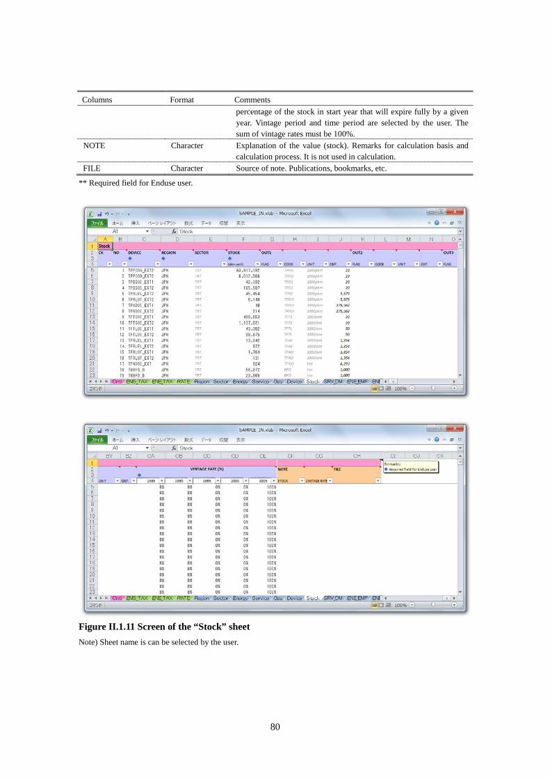
80

Columns Format Comments percentage of the stock in start year that will expire fully by a given year. Vintage period and time period are selected by the user. The sum of vintage rates must be 100%.

NOTE Character Explanation of the value (stock). Remarks for calculation basis and calculation process. It is not used in calculation.

FILE Character Source of note. Publications, bookmarks, etc.

** Required field for Enduse user.

Figure II.1.11 Screen of the “Stock” sheet Note) Sheet name is can be selected by the user.

81

3) SHR_BL and SHR_CM: Maximum/Minimum share of energy device in Baseline and

Countermeasure scenarios

The “SHR_BL” and “SHR_CM” sheets as shown in

Figure II.1.12 specify maximum or minimum share of each energy device in satisfying service

demand, in the baseline and countermeasure scenarios respectively. In the start year, it is necessary

to fill in the specific value for each device. In other simulation years, it is not necessary to fill in the

value except when you wish to set bounds: lower than 100% for maximum share, and greater than

0% for minimum share. AIM/Enduse[ACC] user have to set two types of sheets both baseline case

share (e.g. “SHR_BL”) and countermeasure case share (e.g. “SHR_CM”).

Table II.1.13 Items in the “SHR_BL” sheet and “SHR_CM” sheet


CK *(asterisk) If you leave a blank, the given setting is considered in calculation. If

you wish to exclude a row from calculation, check *(asterisk) for

that row.

NO Integer Number of the data sets. It is an independent number and is not used

in calculation.

DEVICE* Character Device code. The code should be listed in the “Device” sheet.

SERVICE* Character Service code. The code should be listed in the “Service” sheet.

“ALL” can not be used as a code.

REGION* Character Region code. The code should be listed in the “Region” sheet.


SECTOR Character Corresponding sector for the technology listed in the “Device” sheet.

82

SHARE* - Maximum allowable number of years for which a user can specify

share bounds is ten. For the years in between the specified

successive years, the data is linearly interpolated.

[Year] (row4) Integer Year of the share.

[MAX]* Decimal , % Maximum share of the technology (as per cent of final service that

is met by the particular technology). “Blank” is permitted but it is

considered as 100%. The sum of shares of all technologies for a

particular service should be at least 100%.

[MIN]* Decimal , % Minimum share of the technology (as per cent of final service that

is met by the particular technology). “Blank” is permitted but it is

considered as 0%. The sum of shares of all technologies for a

particular service should be at most 100%.

NOTE Character Explanation of the value (service share). Remarks for calculation

basis and calculation process. It is not used in calculation.



83

Figure II.1.12 Screen of the “SHR_BM” sheet Note) Sheet name can be selected by the user.

84

II.1.7 Sheet for Service Demand Data

The “SRV_DM” sheet as shown in Figure II.1.13 specifies the volume of service demand in each

service/region in the selected year. When referring to data, reliable domestic sources of information

(e.g. publications by ministries, government agencies, industry associations, independent research

organizations) would be preferred.

Table II.1.14 Items in the “SRV_DM” sheet





NO Integer Number of the data sets. It is an independent number and is not






SECTOR Character Corresponding sector code listed in the “Sector” sheet.

UNIT Character Corresponding service unit listed in the “Service” sheet.

SERVICE DEMAND* - Maximum allowable number of years for which a user can

specify service demands is ten. For the years in between the

specified successive years, the data is linearly interpolated.

[Year] (row4) Integer Year of the service.

[Value] (row5 and below) Single Service demand quantity for the given service in the given

region in the selected year.

NOTE Character Explanation of the value (service demand). Remarks for

calculation basis and calculation process. It is not used in

calculation.



85

Figure II.1.13 Screen of the “SRV_DM” sheet Note) Sheet name can be selected by the user.

86

II.1.8 Sheets for Energy Data

1) ENE_EMF: Energy emission factor

The “ENE_EMF” sheet as shown in Figure II.1.14 specifies the emission factor for each gas from

each energy type in a given sector and region the selected year. This data should be obtained from

reliable published sources (e.g. publications by ministries, government agencies, industry

associations, independent research organizations). If a user has specified CO2 equivalent (CO2eq) as

the unit for gas in the “Gas” sheet, global warming potential (GWP) factors should be applied to

emissions coefficient of each gas in the “ENE_EMF” sheet. The GWP factors are provided in the

table below.

Table II.1.15 Global Warming Potential

Species Chemical formula

Lifetime (years)

Global Warming Potential

20 years 100 years 500 years

CO2 CO2 variable 1 1 1

Methane * CH4 12±3 56 21 6.5

Nitrous oxide N2O 120 280 310 170

HFC-23 CHF3 264 9100 11700 9800

HFC-32 CH2F2 5.6 2100 650 200

HFC-41 CH3F 3.7 490 150 45

HFC-43-10mee C5H2F10 17.1 3000 1300 400

HFC-125 C2HF5 32.6 4600 2800 920

HFC-134 C2H2F4 10.6 2900 1000 310

HFC-134a CH2FCF3 14.6 3400 1300 420

HFC-152a C2H4F2 1.5 460 140 42

HFC-143 C2H3F3 3.8 1000 300 94

HFC-143a C2H3F3 48.3 5000 3800 1400

HFC-227ea C3HF7 36.5 4300 2900 950

HFC-236fa C3H2F6 209 5100 6300 4700

HFC-245ca C3H3F5 6.6 1800 560 170

Sulphur hexafluoride SF6 3200 16300 23900 34900

Perfluoromethane CF4 50000 4400 6500 10000

Perfluoroethane C2F6 10000 6200 9200 14000

Perfluoropropane C3F8 2600 4800 7000 10100

Perfluorobutane C4F10 2600 4800 7000 10100

Perfluorocyclobutane c-C4F8 3200 6000 8700 12700

Perfluoropentane C5F12 4100 5100 7500 11000

Perfluorohexane C6F14 3200 5000 7400 10700

(Ref.) IPCC homepage (http://unfccc.int/ghg_data/items/3825.php)

87

Table II.1.16 Items in the “ENE_EMF” sheet





NO Integer Number of the data sets. It is an independent number and is

not used in calculation.

ENERGY* Character Energy code. The code should be listed in the “Energy”

sheet.

GAS* Character Gas code. The code should be listed in the “Gas” sheet.

REGION* Character Region code. The code should be listed in the “Region”

sheet or it can be “ALL”. “ALL” means all regions listed

in the “Region” sheet, i.e. the emission factor data applies

to all regions.

SECTOR* Character Sector code. The code should be listed in the “Sector”

sheet or “ALL”. “ALL” means all sectors listed in the

“Sector” sheet, i.e. the emission factor data applies to all

sectors.

UNIT Character Emission factor unit. The unit is automatically selected

from both energy unit listed in the “Energy” sheet and gas

unit listed in the “Gas” sheet.

EMISSION FACTOR* - Maximum allowable number of years for which a user can

specify emission factors is ten. For the years in between

the specified successive years, the data is linearly

interpolated.

[Year] (row4) Integer Year of the energy emission factor.

[Value] (row5 and below) Single Emission factor of the particular gas from the particular

energy type in the given sector and region in the selected

year.

NOTE Character Explanation of the value (emission factor). Remarks for


calculation.



88

Figure II.1.14 Screen of the “ENE_EMF” sheet Note) Sheet name can be selected by the user.

89

2) ENE_PRC: Energy Price

The “ENE_PRC” sheet as shown in Figure II.1.15 specifies the energy price in each

energy/region/sector in the selected year. Data should be obtained from reliable published sources

(e.g. publications by ministries, government agencies, industry associations, independent research

organizations).

Table II.1.17 Items in the “ENE_PRC” sheet







ENERGY* Character Energy code. The code should be listed in the “Energy” sheet.

REGION* Character Region code. The code should be listed in the “Region” sheet

or it can be “ALL”. “ALL” means all regions listed in the

“Region” sheet. i.e. the energy price data applies to all regions.

SECTOR* Character Sector code. The code should be listed in the “Sector” sheet or

is can be “ALL”. “ALL” means all sectors listed in the

“Sector” sheet. i.e. the energy price data applies to all sectors.

UNIT Character Energy price unit. The unit is automatically selected from both

energy unit listed in the “Energy” sheet and monetary unit in

the “Cntl” sheet.

ENERGY PRICE* - Maximum allowable number of years for which a user can

specify energy price is ten. For the years in between the

specified successive years, the data is linearly interpolated.

[Year] (row4) Integer Year of the energy price.

[Value] (row5 and below) Single Energy price of the particular energy type in the given sector

and region in the selected year.

NOTE Character Explanation of the value (energy price). Remarks for


calculation.



90

Figure II.1.15 Screen of the “ENE_PRC” sheet Note) Sheet name can be selected by the user.

91

II.1.9 Optional Sheets

1) MR: Region class

The “MR” sheet as shown in Figure II.1.16 specifies the regional group classification with some

regions listed in the “Region” sheet. This table is optionally used when a user wants to balance

energy and material among certain regions (e.g. for North America considering USA and Canada,

and for European Union 25 (EU25) considering EU15 and EU10), a user can make a group of

countries/regions by using this table).

Table II.1.18 Items in the “MR” sheet

Columns Format Comments CK *(asterisk) If you leave a blank, the given setting is considered in

calculation. If you wish to exclude a row from calculation, check *(asterisk) for that row.


REGION* Character Select a region code listed in the “Region” sheet. SECTOR* Character Select a sector code listed in the “Sector” sheet. REGION CLASS (MR)* Character Code of the group of countries/regions to which the

particular country/region belongs. A user can select any code but it should be different from the codes used in the “Region” sheet. “ALL” can not be used as a code.


Figure II.1.16 Screen of the “MR” sheet Note) Sheet name can be selected by the user.

92

2) INT: Internal service and internal energy (Optional)

The “INT” sheet as shown in Figure II.1.17 specifies the relationship between internal energy and

internal service. When a certain device consumes an input of energy or service which is a service or

energy output from another device, the user needs to specify the linkage or equivalence between that

input and that output in this sheet. (e.g. When “gasoline” and “biofuel” produce “biogasoline”, and

“biogasoline” is used for “passenger transportation service”, the user can use group code(INT) for

“biogasoline” in this sheet.)

Table II.1.19 Items in the “INT” sheet Columns Format Comments



SERVICE* Character Select a service code listed in the “Service” sheet which is equivalent or same as an internal energy.

ENERGY* Character Select an energy code listed in the “Energy” sheet which equivalent or same as an internal service.

GROUP CODE (INT)* Character Code used for the combination of internal energy and internal service. Any code can be selected by the user.


Figure II.1.17 Screen of the “INT” sheet Note) Sheet name can be selected by the user.

Device 1Energy/Service(In)

Service(Out)

INTDevice 2Energy/Service

(In)Service

(Out)

93

3) MR_INT: Relation between region/MR and INT (Optional)

The “MR_INT” sheet as shown in Figure II.1.18 specifies all combinations of region (including

regional group defined in the “MR” sheet) and internal service and internal energy (INT). (e.g. In

case a user defines “biogasoline” as internal service and internal energy in the “INT” sheet, then, the

regions which use biogasoline are specified in this sheet.)

Table II.1.20 Items in the “MR_INT” sheet







GROUP(INT)* Character Code of combination of internal service and internal

energy listed in the “INT” sheet.

REGION, GROUP(MR)* Character Region code listed in the “Region” sheet or region group

code listed in the “MR” sheet. “ALL” can not be used as a

code.


Figure II.1.18 Screen of the “MR_INT” sheet Note) Sheet name can be selected by the user.

94

4) M_N: Technology group (Optional)

The “M_N” sheet as shown in Figure II.1.19 specifies all groups of devices or technologies. If a user

wants to set a maximum or minimum bound on the share of a certain group of technologies for a

particular service in a given sector and region, such a user should use this sheet to define the

technology groups. With regard to the setting of minimum or maximum shares of the defined

technology group, the user must enter the data in the “OMMX” sheet. (e.g. When a user wants to set

minimum or maximum share for the total of “High-efficiency gasoline passenger car” and “Plug-in

hybrid gasoline car”, the group code(N) for those devices must be defined in this sheet.)

Table II.1.21 Items in the “M_N” sheet




DEVICE* Character Device code. The code should be listed in a “Device” sheet. GROUP CODE(N)* Character Technology group code. A user can select any code. “ALL”

can not be used as a code.


Figure II.1.19 Screen of the “M_N” sheet Note) Sheet name can be selected by the user.

95

5) OMMX: Max/min allowable service share of technology group (Optional)

The “OMMX” sheet as shown in Figure II.1.20 specifies the maximum or minimum allowable

service share of a technology group. (e.g. In case a user wants to set an upper limit or lower limit of

service share for the total high-efficiency cars; HV, EV, PHV, FC, first a group code (N) for all these

devices must be defined in the “M_N” sheet, and then, the user must specify the minimum or

maximum bounds on share of that group in this sheet.)

Table II.1.22 Items in the “OMMX” sheet




GROUP(N)* Character Technology group code. The code should be listed in the “M_N” sheet.

REGION* Character Region code. The code should be listed in the “Region” sheet. SECTOR Character Corresponding sector code listed in the “Sector” sheet. SERVICE* Character Service code. The code should be listed in the “Service”

sheet. MAX/MIN* Two choices "MAX" or "MIN". One of these two options can be

selected from a pull-down menu. SHARE (%)* - Maximum allowable number of years for which a user can

specify the bounds on share is ten. For the years in between the specified successive years, the data is linearly interpolated.

[Year] (row4) Integer Year of the service share of technology group. [Value] (row5 and blow) Decimal, % Upper limit or lower limit of the service share of the

particular technology group (N) in the selected year. NOTE Character Explanation of the value (allowable service share).

Remarks for calculation basis and calculation process. It is not used in the calculation.



96

Figure II.1.20 Screen of the “OMMX” sheet Note) Sheet name can be selected by the user.

97

6) MQ: Emission constraint group of sectors/regions (Enduse Only) (Optional)

The “MQ” sheet as shown in Figure II.1.21 specifies all combinations of regions and sectors for

defining emission constraint group. If a user wants to set the maximum or minimum emission limit

for a group of regions and sectors, this sheet must be used to define that group.

Table II.1.23 Items in the “MQ” sheet




REGION (ALL available)** Character Region code. The code should be listed in the “Region” sheet or “ALL”. “ALL” means all regions listed in the “Region” sheet.

SECTOR (ALL available)** Character Sector code. The code should be listed in the “Sector” sheet or “ALL”. “ALL” means all sectors listed in the “Sector” sheet.

GROUP CODE (MQ)** Character Code for the group of regions/sectors for which emission constraint needs to be applied. Any code can be selected by the user. “ALL” can not be used as a code.

**Required field for Enduse users.

Figure II.1.21 Screen of the “MQ” sheet Note) Sheet name can be selected by the user.

98

7) MG: Emission constraint group of gases (Enduse Only) (Optional)

The “MG” sheet as shown in Figure II.1.22 specifies all combinations of gases for defining emission

constraint groups. If a user wants to set the maximum or minimum emission limit for a group of

gases, this sheet must be used to define such a group.

Table II.1.24 Items in the “MG” sheet




GAS(ALL available)** Character Gas code. The code should be listed in the “Gas” sheet, or “ALL”. “ALL” means all gases listed in the “Gas” sheet.

GROUP CODE (MG)** Character Code for the group of gases for which emission constraint needs to be defined. Any code can be selected by the user. “ALL” can not be used as a code.

**Required field for Enduse users.

Figure II.1.22 Screen of the “MG” sheet Note) Sheet name can be selected by the user.

99

8) QMAX: Maximum allowable emission of gas or group of gases (Enduse Only)

(Optional)

The “QMAX” sheet as shown in Figure II.1.23 specifies the maximum allowable emission limit on a

gas or a group of gases in a given region/sector or group of regions/sectors. (e.g. In case a user wants

to set an upper limit on emission of a gas or group of gases in a specific region/sector or a group of

regions/sectors, the codes for the corresponding codes for groups of gases (gas(MG)) and

regions/sectors (region/sector(MQ)) must first be defined in the sheets “MG” and “MQ” respectively,

and then the user must specify the maximum emission limit in this sheet.)

Table II.1.25 Items in the “QMAX” sheet







GROUP(MQ)** Character Group code for regions/sectors for emission constraint. The

code should be listed in a “MQ” sheet.

GROUP(MG)** Character Group code for gases for emission constraint. The code should

be listed in a “MG” sheet.

QUANTITY (gas unit)** - Maximum allowable number of years for which a user can

specify the emission limits is ten. For the years in between

the specified successive years, the data is linearly

interpolated.

[Year] (row4) Integer Year of the gas emission.

[Value] (row5 and below) Single Upper limit of allowable gas emission in the selected year.

NOTE Character Explanation of the value (allowable gas emission amount).

Remarks for calculation basis and calculation process. It is



** Required field for Enduse users.

100

Figure II.1.23 Screen of the “QMAX” sheet Note) Sheet name can be selected by the user.

101

9) ME: Energy constraint group of regions/sectors (Optional)

The “ME” sheet as shown in Figure II.1.23 specifies all groups/combinations of regions/sectors for

which energy constraints need to be specified. If a user wants to set the maximum or minimum limit

on energy supply (for a particular energy type) in a region/sector or a group of regions/sectors, this

sheet must be used to define such a group. (e.g. When a user wants to set the upper limit or lower

limit of energy supply for “biogasoline” in a set of regions and sectors, that set if regions/sectors

must be defined with an energy constraint group code(ME) in this sheet.)

Table II.1.26 Items in the “ME” sheet







REGION (ALL available)* Character Region code. The code should be listed in the “Region” sheet, or

“ALL”. “ALL” means all regions listed in the “Region” sheet.

SECTOR (ALL available)* Character Sector code. The code should be listed in the “Sector” sheet, or

“ALL”. “ALL” means all sectors listed in the “Sector” sheet.

GROUP CODE (ME)* Character Code for a combination of region and sector or a group of

regions and sectors for which an energy supply limit needs to

be specified. Any code can bee seleted by the user. “ALL” can

not be used as a code.


Figure II.1.24 Screen of the “ME” sheet Note) Sheet name can be selected by the user.

102

10) EMAX: Max/Min allowable energy supply limit the regions/sectors of energy constraint

group (Optional)

The “EMAX” sheet as shown in Figure II.1.25 specifies the maximum or minimum allowable limits

on energy supply in the defined combinations of region/sector or group of regions/sectors. (e.g. In

case a user wants to set the upper limit or lower limit of energy supply for “biogasoline”, first the

combinations of region and sector need to be defined with group code(ME) in the “ME” sheet, and

then, the minimum or maximum energy supply limit for each group must be specified in this sheet.)

Table II.1.27 Items in the “EMAX” sheet







GROUP(ME)* Character Energy constraint group code (of combination of

region/sector). The code should be listed in the “ME” sheet.

ENERGY* Character Energy code. The code should be listed in the “Energy” sheet.

MAX/MIN* Two choices "MAX" or "MIN". One of these two options can be

selected from a pull-down menu.

QUANTITY (ene.unit)* - Maximum allowable number of years for which a user can

specify the energy supply limits is ten. For the years in

between the specified successive years, the data is linearly

interpolated.

[Year] (row4) Integer Year of the energy supply.

[Value] (row5 and below) Single Upper limit or lower limit on allowable energy supply in

the selected year.

NOTE Character Explanation of the value (allowable energy supply).





103

Figure II.1.25 Screen of the “EMAX” sheet Note) Sheet name can be selected by the user.

104

11) SGMX: Max/Min allowable regional service share (Optional)

The “SGMX” sheet as shown in Figure II.1.26 specifies the maximum or minimum allowable

regional service share. If a user wants to set the upper limit or lower limit of regional service share in

a specific region/sector, such a user should use this sheet. (e.g. the limit of natural gas supply in a

certain region)

Table II.1.28 Items in the “SGMX” sheet












SHARE (%)* - Maximum allowable number of years for which a user can

specify the limits on regional service share is ten. For the

years in between the specified successive years, the data is

linearly interpolated.

[Year] (row4) Integer Year of the regional service share.

[Value] (row5 and below) Decimal, % Upper limit or lower limit of allowable service supply in

the selected year.

NOTE Character Explanation of the value (allowable regional service share).


not used in the calculation.



105

Figure II.1.26 Screen of the “SGMX” sheet Note) Sheet name can be selected by the user.

106

12) ROMX: Max/min allowable stock quantity (Enduse Only) (Optional)

The “ROMX” sheet as shown in Figure II.1.27 specifies the maximum or minimum allowable limit

on the stock quantity of each device. If a user wants to set upper limit or lower limit of stock

quantity for a certain device in a specific region/sector in the selected year, it must be specified in

this sheet.

Table II.1.29 Items in the “ROMX” sheet



calculation. If you wish to exclude a row from

calculation, check *(asterisk) for that row.

NO Integer Number of the data sets. It is an independent number and

is not used in calculation.

REGION** Character Region code. The code should be listed in the “Region”

sheet.


DEVICE** Character Device code. The code should be listed in the “Device”

sheet.

MAX/MIN** Two choices "MAX" or "MIN". One of these two options can be


QUANTITY (dev.unit)** - Maximum allowable number of years for which a user

can specify the limits on stock quantity is ten. For the

years in between the specified successive years, the data

is linearly interpolated.

[Year] (row4) Integer Year of the stock quantity.

[Value] (row5 and below) Single Upper limit or lower limit of allowable stock quantity in

the selected year.

NOTE Character Explanation of the value (allowable stock quantity).

Remarks for calculation basis and calculation process. It

is not used in the calculation.



107

Figure II.1.27 Screen of the “ROMX” sheet Note) Sheet name can be selected by the user.

108

13) TUMX: Max/min allowable recruited quantity (Optional)

The “TUMX” sheet as shown in Figure II.1.28 specifies the maximum or minimum allowable limit

on the recruited (or newly installed) quantity of each device. If a user wants to set the upper limit or

lower limit of recruited (or newly installed) quantity of certain device in a specific region/sector in

the selected year, it must be specified in this sheet.

Table II.1.30 Items in the “TUMX” sheet









DEVICE* Character Device code. The code should be listed in the “Device” sheet.



QUANTITY (dev.unit)* - Maximum allowable number of years for which a user can

specify the limits on recruited quantity of a device is ten.

For the years in between the specified successive years, the

data is linearly interpolated.

[Year] (row4) Integer Year of the recruited quantity.

[Value] (row5 and below) Single Upper limit or lower limit of the allowable recruited

quantity of the particular device in the selected year.

NOTE Character Explanation of the value (allowable recruited quantity).


not used in the calculation.



109

Figure II.1.28 Screen of the “TUMX” sheet Note) Sheet name can be selected by the user.

110

14) ETMX: Max/min allowable annual rate of change in recruited quantity (Optional)

The “ETMX” sheet as shown in Figure II.1.29 specifies the maximum or minimum allowable annual

rate of change in recruited quantity of a device. A positive rate implies growth of recruited quantity,

whereas a negative rate implies decline. If a user wants to set the upper limit or lower limit of annual

growth rate of recruited quantity of certain device in a region/sector in the selected year, it must be

specified in this sheet.

Table II.1.31 Items in the “ETMX” sheet




REGION* Character Region code. The code should be listed in the “Region” sheet. SECTOR Character Corresponding sector code listed in the “Sector” sheet. DEVICE* Character Device code. The code should be listed in the “Device” sheet. MAX/MIN* Two choices "MAX" or "MIN". One of these two options can be

selected from a pull-down menu. RATE (%) - Maximum allowable number of years for which a user can

specify the limits on annual rate of change in recruited quantity of a device is ten. For the years in between the specified successive years, the data is linearly interpolated.

[Year] (row4) Integer Year of the rate of change in the recruited quantity. [Value] (row5 and below) Decimal, % Upper limit or lower limit of the allowable annual growth

rate of recruited quantity in the selected year. NOTE Character Explanation of the value (allowable change rate of

recruited quantity). Remarks for calculation basis and calculation process. It is not used in the calculation.



111

Figure II.1.29 Screen of the “ETMX” sheet Note) Sheet name can be selected by the user.

112

15) DEV_IMP: Energy device improvement (Enduse Only) (Optional)

The “DEV_IMP” sheet as shown in

Figure II.1.30 specifies the efficiency improvement of a device in the production of a specific service,

use of a specific energy, or non-energy/non-combustion related emission of a specific gas. If a user

wants to set such an efficiency improvement of the selected device, it must be specified in this sheet.

The data of a “DEV_IMP” sheet is valid only when the corresponding device is defined in the

“Device” sheet (e.g. if a user wants to describe 5% increase in efficiency of a certain device in terms

of use of a particular energy in the ten year period from 2005 to 2015, then the rate of improvement

must be specified as 100% in 2005 and 95% in 2015).

113

Table II.1.32 Items in the “DEV_IMP” sheet








sheet.

ITEM** List Code of the item in which improvement needs to be

described for the selected device. It can be “OUT” for

output service (OUT1 to OUT4), “IN” for input energy

(IN1 to IN8), or “GAS” for gas emitted independent of

energy/combustion (GAS1 to GAS8). One of these items

can selected from a pull down menu.

RATE (%)** - Maximum allowable number of years for which a user

can specify the rate of improvement of a device is ten.

For the years in between the specified successive years,

the data is linearly interpolated.

[Year] (row4) Integer Year of the efficiency improvement.

[Value] (row5 and below) Decimal, % Rate of efficiency improvement of the selected device in

the production/use/emission of the selected item. In the

calculation, efficiency improvement rate in a particular

year is normalized relative to the value or rate specified at

the extreme left (which is normally the value of the start

year of simulation).

NOTE Character Explanation of the value (technology efficiency

improvement rate). Remarks for calculation basis and

calculation process.. It is not used in the calculation.



114

Figure II.1.30 Screen of the “DEV_IMP” sheet Note) Sheet name can be selected by the user.

115

16) DEV_CST: Detailed technology cost (Optional)

The “DEV_CST” sheet as shown in

Figure II.1.31 specifies the initial capital investment cost or O&M cost of a certain device in each

region/sector. If a user wants to set a region specific initial/O&M costs of a certain device in the

selected year, it must be specified in this sheet. If initial/O&M cost of a certain device applies to all

regions/sectors, please specify that cost data only in the “Device” sheet.

Table II.1.33 Items in the “DEV_CST” sheet


116







sheet.


DEVICE* Character Device code. The code should be listed in the “Device”

sheet.

INITIAL/O&M* Two choices “INITIAL” or “O&M”. One of these two options can be


COST* - Maximum allowable number of years for which a user

can specify the initial/O&M costs of a device in a

region/sector is ten. For the years in between the

specified successive years, the data is linearly

interpolated.

[Year] (row4) Integer Year of the device cost.

[Value] (row5 and below) Single The initial cost or O&M cost of a certain device in a

certain region/sector. In AIM/Enduse[ACC] model run,

program reads only the value at the extreme left.

NOTE Character Explanation of the value (detailed technology cost).

Remarks for calculation basis and calculation process. It




117

Figure II.1.31 Screen of the “DEV_CST” sheet Note) Sheet name can be selected by the user.

118

17) PHI_T: Social service improvement (Optional)

The “PHI_T” sheet as shown in Figure II.1.32 specifies the social service improvement in a

service/region/sector. This parameter indicates a change in consumption of a service as a result of

improvement in the end-user lifestyle or in the method of use or delivery of that service. If a user

wants to set a social service improvement rate of a certain service in a certain region/sector, it must

be specified in this sheet. If no value is entered, the default value is assumed as 100% in the model.

The following example explains this parameter.

Image of PHI_T

There are two devices descried in the “Device” sheet: device1 (“Dev1”) which outputs 10

service (“Out1”) consuming 10 energy (“In1”) and device2 which outputs 10 service (“Out1”)

consuming 9 energy (“In2”).

Now, in a “PHI_T” sheet, if a user set 100% increase in a social service improvement only for

“Out1” for the next fifteen years (2020), the service output of each device unit becomes double,

therefore, calculation is executed considering “Dev1” outputs 10 service consuming 10 energy

in 2005 and outputs 20 service consuming 10 energy in 2020; “Dev2” outputs 10 service

consuming 9 energy in 2005 and outputs 20 service consuming 9 energy in 2020.

10

Dev110 10

Dev1 20

In1Out1

In Device Out

In1Out1

2005:1+PHI=100%

2020:1+PHI=200%

9

Dev29

10

Dev2 20

In2

In2

119

Table II.1.34 Items in the “PHI_T” sheet







REGION* Character Region code. The code listed in the “Region” sheet.


SERVICE* Character Service code. The code should be listed in the “Service”

sheet.

RATE (%)* - Maximum allowable number of years for which a user

can specify the social service improvement rate is ten.

For the years in between the specified successive years,

the data is linearly interpolated.

[Year] (row4) Integer Year of the social service improvement.

[Value] (row5 and below) Decimal, % Social service improvement rate of a certain service in a

certain region/sector. In AIM/Enduse[ACC] model run,

program reads only the value at the extreme left.

NOTE Character Explanation of the value (social service improvement

rate). Remarks for calculation basis and calculation

process. It is not used in the calculation.



Figure II.1.32 Screen of the “PHI_T” sheet Note) Sheet name can be selected by the user.

120

18) GAM_T: Operating efficiency improvement (Optional)

The “GAM_T” sheet as shown in Figure II.1.33 specifies the operating efficiency of each device. If a

user wants to describe a change in the operating efficiency of a device in a region/service, it must be

specified in this sheet. If no value is entered, the default value is assumed as 100% in the model.

The following example explains this parameters.

Image of GAM_T

There are two devices descried in the “Device” sheet: device1 (“Dev1”) which outputs 10

service (“Out1”) consuming 10 energy (“In1”) and device2 which outputs 10 service (“Out1”)

consuming 10 energy (“In2”).

Now, in a “GAM_T” sheet, if a user sets 70% of operating efficiency rate for both “Dev1” and

“Dev2” in the start year (2005) and sets twice the rate of “Dev1” for the next fifteen years,

calculation is executed considering “Dev1” output 7 service consuming 7 energy in 2005 and

output 14 service consuming 14 energy in 2020; “Dev2” outputs 7 service consuming 7 energy

and outputs 7 service consuming 7 energy (no change).

If a user sets the increase in the operating efficiency rate of a certain device in a different

region/service, the cost (annualized investment cost, operating cost, etc.) will be much reduced.

14

Dev17 7

Dev1 14

In1Out1

In Device Out

In1Out1

2005:1+GAM=70%(Dev1, Dev2)

2020:1+GAM=140%（Dev1)

1+GAM=70%（Dev2)

7

Dev27

7

Dev2 7

In2

In2

121

Table II.1.35 Items in the “GAM_T” sheet





SECTOR Character Corresponding sector code listed in the “Sector” sheet. DEVICE* Character Device code. The code should be listed in the “Device”

sheet. RATE (%)* - Maximum allowable number of years for which a user can

specify the device operating efficiency rate is ten. For the years in between the specified successive years, the data is linearly interpolated.

[Year] (row4) Integer Year of the operating efficiency improvement. [Value] (row5 and below) Decimal, % Operating efficiency rate in a certain device in a

region/sector. In AIM/Enduse[ACC] model run, program reads only the value at the extreme left.

NOTE Character Explanation of the value (technology operating efficiency rate). Remarks for calculation basis and calculation process. It is not used in the calculation.



Figure II.1.33 Screen of the “GAM_T” sheet Note) Sheet name can be selected by the user.

122

19) XI_T: Countermeasure for energy efficiency change by maintenance (Optional)

Change in life style and method of use and maintenance of devices can result in conservation of

energy at end-use stage. The “XI_T” sheet as shown in Figure II.1.34 specifies the countermeasure

for change in energy efficiency by improved maintenance. If a user wants to set the countermeasure

for improvement in energy efficiency due to better maintenance of a device in a region/sector, it

must be specified in this sheet. If no value is entered by, the default value of energy efficiency

change is assumed as 0% in the model.

Table II.1.36 List of columns in “XI_T”








sheet.


DEVICE* Character Device code. The code should be listed in the “Device”

sheet.

RATE (%)* - Maximum allowable number of years for which a user can

specify the energy efficiency by maintenance is ten. For

the years in between the specified successive years, the

data is linearly interpolated.

[Year] (row4) Integer Year of the energy efficiency by maintenance.

[Value] (row5 and below) Decimal, % Rate of energy efficiency change by maintenance of a

device in a certain region/sector. In AIM/Enduse[ACC]

model run, program reads only the value at the extreme

left.

NOTE Character Explanation of the value (rate of energy efficiency change

by maintenance). Remarks for calculation basis and

calculation process. It is not used in the calculation.



123

Figure II.1.34 Screen of the “XI_T” sheet Note) Sheet name can be selected by the user.

124

20) SCN_T: Subsidy rate for recruited technology (Enduse Only) (Optional)

The “SCN_T” sheet as shown in Figure II.1.35 specifies the rate of subsidy on the initial (capital)

cost and operational (O&M) cost of a recruited technology in a region/sector. If a user wants to

describe or apply a subsidy on initial cost or O&M cost of a device in a region/sector, it must be

specified in this sheet. If no value is entered, the default value of subsidy rate is assumed as 0% in

the model, i.e. no subsidy.

Table II.1.37 Items in the “SCN_T” sheet







REGION** Character Region code. The code should be listed in the “Region”

sheet.



sheet.

INITIAL/O&M** Two choices "INITAL" or "O&M". One of these two options can be


RATE (%)** - Maximum allowable number of years for which a user

can specify the rate of subsidy on a recruited device is

ten. For the years in between the specified successive

years, the data is linearly interpolated.

[Year] (row4) Integer Year of the subsidy rate.

[Value] (row5 and below) Decimal, % Subsidy rate for initial/O&M cost of the recruited

technology in a certain region/sector.

NOTE Character Explanation of the value (subsidy rate for recruited

technology). Remarks for calculation basis and

calculation process. It is not used in the calculation.



125

Figure II.1.35 Screen of the “SCN_T” sheet Note) Sheet name can be selected by the user.

126

21) M_NQ: Observation sector for gas emission comparison (Optional)

The “M_NQ” sheet as shown in Figure II.1.36 specifies the combinations of regions and sectors for

which a user wishes to compare the emission of a gas in the model simulation results with that in the

observed/recorded/published data. If a user wants to do a calibration check between simulation

results and observed gas emissions in the simulation start year for a particular gas in a region/sector,

that combination of region and sector must be defined with a new code in this sheet.

Table II.1.38 Items in the “M_NQ” sheet








SECTOR* Character Sector code. The code should be listed in the “Sector” sheet.

GROUP CODE(NQ)* Character Code for the selected combination of region and sector for

which the simulation results of emission of certain gases in

the start year need to be compared/calibrated with the

observed/published data. Any code can be selected by the

user. “ALL” can not be used as a code.


Figure II.1.36 Screen of the “M_NQ” sheet Note) Sheet name can be selected by the user.

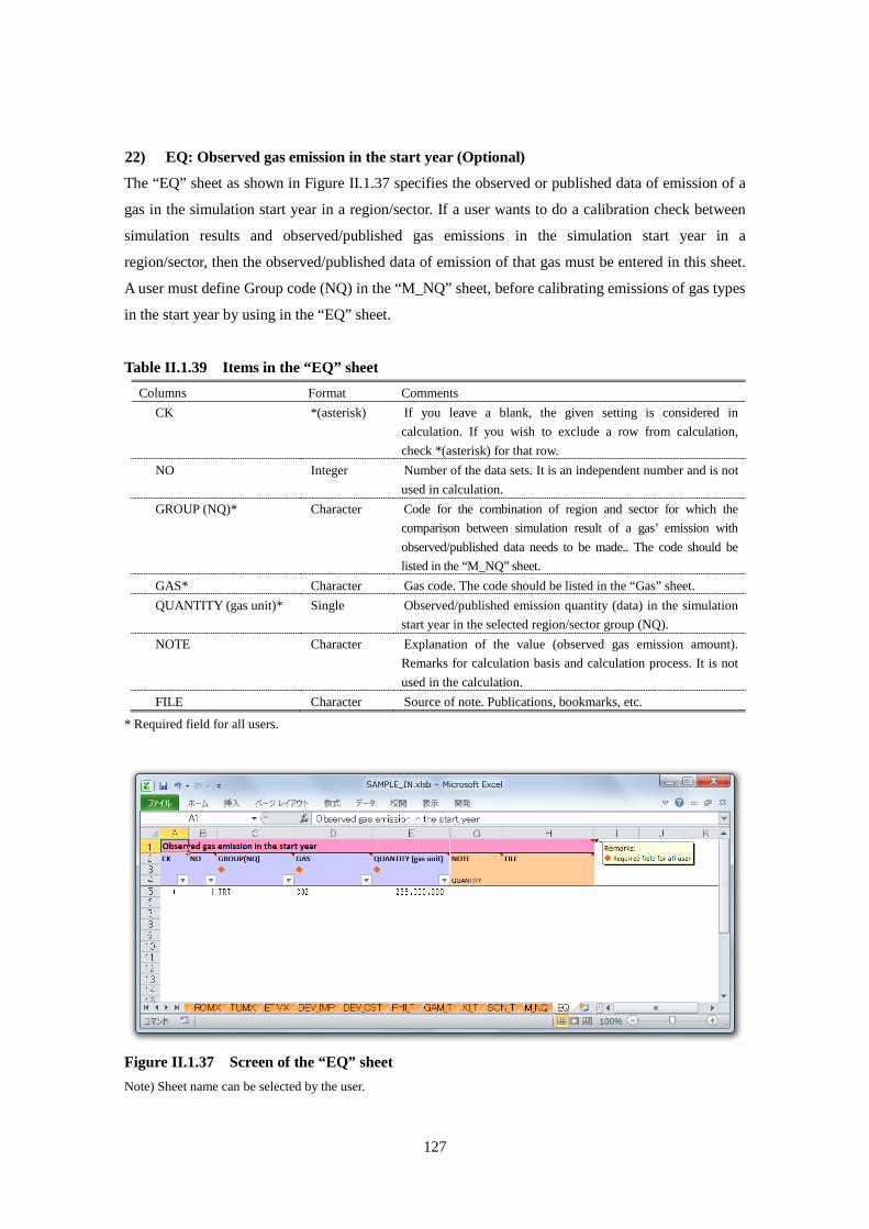
127

22) EQ: Observed gas emission in the start year (Optional)

The “EQ” sheet as shown in Figure II.1.37 specifies the observed or published data of emission of a

gas in the simulation start year in a region/sector. If a user wants to do a calibration check between

simulation results and observed/published gas emissions in the simulation start year in a

region/sector, then the observed/published data of emission of that gas must be entered in this sheet.

A user must define Group code (NQ) in the “M_NQ” sheet, before calibrating emissions of gas types

in the start year by using in the “EQ” sheet.

Table II.1.39 Items in the “EQ” sheet Columns Format Comments



GROUP (NQ)* Character Code for the combination of region and sector for which the comparison between simulation result of a gas’ emission with observed/published data needs to be made.. The code should be listed in the “M_NQ” sheet.

GAS* Character Gas code. The code should be listed in the “Gas” sheet. QUANTITY (gas unit)* Single Observed/published emission quantity (data) in the simulation

start year in the selected region/sector group (NQ). NOTE Character Explanation of the value (observed gas emission amount).

Remarks for calculation basis and calculation process. It is not used in the calculation.



Figure II.1.37 Screen of the “EQ” sheet Note) Sheet name can be selected by the user.

128

II.2 GAMS model execution

BAT file (“AIM_Enduse.BAT” or “AIM_MAC.BAT”) is an executable file created by “(file

name)_IN.xlsb”. “(file name)_IN.xlsb” also creates data sets for GAMS Program in the specified

folder (e.g. C:¥Enduse_Global¥SAMPLE¥Enduse) (Note: folder name and folder location is set by a

user, these are listed in the “Cntl” sheet in“(file name)_IN.xlsb”.)

Figure II.2.1 “AIM_Enduse.BAT” and data set in the selected folder

Open “AIM_Enduse.BAT”.

GAMS program (“AIM_CMB.gms”) starts calculation. (See Figure II.2.2)

Figure II.2.2 After opening “AIM_Enduse.BAT”, the GAMS model calculation starts

129

If the run finishes successfully, the following result/output files (csv files) are created or

overwritten in the same folder (See Figure II.2.3).

-Detail output file “(file name)_detail.csv”

-Output file of cost per unit emission reduction “(file name)_cost.csv”

-Output file of emission factor “(file name)_emsfc.csv”

-Output file of internal service and energy balance “(file name)_internal.csv”

Figure II.2.3 Output files created from GAMS program

AIM/Enduse software displays simulation results and abatement cost curve result in the files “(file

name)_PIVOT.xlsb” and “(file name)_ACC.xlsb” respectively.

The following sections (section 2.5 and section 2.6) explain the output files “(file name)_PIVOT.xlsb”

and “(file name)_ACC.xlsb”.

130

II.3 Description of “(file name)_PIVOT.xlsb”

II.3.1 Overview

“(file name)_PIVOT.xlsb” is a user interface to show the output from GAMS program

(AIM_Enduse.gms or AIM_MAC.gms). Microsoft Excel 2007 is to desirable for the operating

environment (note: the user whose operating environment is Excel 2003 should use “(file

name)_PIVOT.xls” in “Excel2003”).

“(file name)_PIVOT.xlsb” comprises “Cntl” and 6 component sheets, viz. “PvtT_Enduse”,

“PvtG_Enduse”, “Region_Enduse”, “PvtT_ACC”, “PvtG_ACC”, and “Region_ACC”.

The process of use of “(file name)_PIVOT.xlsb” is as follows:

1) Open “(file name)_PIVOT.xlsb” (e.g. SAMPLE_PIVOT.xlsb). Any file name and file location

can be selected by a user.

2) Enter data in the “Cntl” sheet. The “Region” sheet (“Region_Enduse” for AIM/Enduse model

run, “Region_ACC” for AIM/Enduse[ACC] model run) is optional.

3) After finished entering data in the “Cntl” sheet, please select “Run”. If execution finishes

successfully, a “PvtT” sheet (“PvtT_Enduse” for AIM/Enduse model run; “PvtT_ACC” for

AIM/Enduse[ACC]) and a “PvtG” sheet (“PvtG_Enduse” for AIM/Enduse model; “PvtG_ACC”

for AIM/Enduse[ACC]) are automatically refreshed and program activates the “PvtT” sheet.

131

II.3.2 Control Sheet

“(file name)_PIVOT.xlsb“ loads “(case name)_detail.csv” and shows pivot table by executing

Excel/VBA. The “Cntl” sheet as shown in Figure II.3.1 appears on clicking at “(file

name)_PIVOT.xlsb“. User has to fill in the items listed in Table II.3.1.

Table II.3.1 Items in the “Cntl” sheet

Columns Format Comments CK *(asterisk) If you leave a blank, the data is imported from the “(case

name)_detail.csv”. If you wish to exclude an item, check *(asterisk) in that row.


ITEM - Item code listed in “(case name)_detail.csv”. description - Description of the item. SCALE Single Factor for the unit conversion. It is used for unit conversion between

original unit and displayed unit in the output results. CSV UNIT Character Original unit. DISPLAY UNIT Character Display unit.


After filling the above table, the user needs to fill in the following tables as necessary.. Upper table is

for Enduse user and bottom table is for Enduse[ACC] user.

132

Table II.3.2 Items in the “Cntl” sheet (For Enduse)

Columns Format Comments CK *(asterisk) If you leave a blank, the data is imported from the “(case

name)_detail.csv”. If you wish to exclude an item, check *(asterisk) in that row.

NO Integer Number of the data sets. It is automatically described and is not used in calculation.

CASE Character Case name for analysis. Every name must be unique in the list. description Character Case description. It is not used in calculation. YEAR - -

All *(asterisk) If you leave this blank, all results are imported from “(case name)_detail.csv”. Check *(asterisk) to a row if you wish to exclude these results in display.

_base *(asterisk) If you leave this blank, “_base” results are imported from “(case name)_detail.csv”. Check *(asterisk) to a row if you wish to exclude these results in display.

Selected Character If you want to pick up results of the specific year(s) (e.g. 2005, 2010, 2020, 2030), then enter that/those year(s) in the cell. Use “+” to separate two successive years.

FILE LOCATION Character Location of “(case name)_detail.csv”. Click the left cell (blue colored) to find a file you want to import.

Table II.3.3 Items in the “Cntl” sheet (For ACC) Columns Format Comments

CK *(asterisk) If you leave a blank, the data is imported from the “(case name)_detail.csv”. If you wish to exclude an item, check *(asterisk) in that row.

NO Integer Number of the data sets. It is automatically described and is not used in calculation.

CASE Character Case name for analysis. Every name must be unique in the list. description Character Case description. It is not used in calculation. YEAR - -

START *(asterisk) If you leave this blank, results of simulation start year are imported from “(case name)_detail.csv”. Check *(asterisk) to a row if you wish to exclude these results in display.

B.L. *(asterisk) If you leave this blank, results of the baseline are imported from “(case name)_detail.csv”. Check *(asterisk) to a row if you wish to exclude these results in display.

C.M. Character If you leave the blank, results of the countermeasure case are imported from “(case name)_detail.csv”. Check *(asterisk) to a row if you wish to exclude these results in display.

FILE LOCATION Character Location of “(case name)_detail.csv”. Click the left cell (blue colored) to find a file you want to import.

133

II.3.3 Component Sheets

1) PvtT: Pivot table sheet

After finishing data entry in the “Cntl” sheet, click the “Run” button. If the run finishes successfully,

the pivot table (“PvtT_Enduse” for AIM/Enduse model; “PvtT_ACC” for AIM/Enduse[ACC]

model) is refreshed automatically. If a user clicks the filter on the upper side of the form as shown in

Figure II.3.2, it shows the list. For example, if a user selects “EMSD”, it shows direct emission

results.

Table II.3.4 Filter of pivot table Filter Code Content Kind STK Stock quantity

DEV Operating quantity SRV Service supply ENG Energy consumption EMSD Direct emission quantity EMSI*2 Indirect emission quantity CST Cost RCT Recruited (newly installed) quantity

Item Kind = CST RCA Total annualized investment cost RCI Total initial investment cost MDA* Total annualized cost of exchanging removal process MDI* Total initial cost of exchanging removal process MNT Total operating cost including energy cost, material cost,

maintenance cost etc. TXE*1 Energy tax payment TXM Emission tax payment DLC*2 Total cost of emission reduction from baseline

DLCP*2 Total cost of emission reduction from baseline, excluding negative cost

AC*2 Cost per unit emission reduction Kind = STK - - Kind = DEV - -

Kind = SRV (Service Type) The code listed in the “Service” sheet in “(case

name)_IN.xlsb”

Kind = ENG (Energy Type) The code listed in the “Energy” sheet in “(case

name)_IN.xlsb” Kind = EMSD (Gas Type) The code listed in the “Gas” sheet in “(case name)_IN.xlsb” Kind = EMSI*2 (Gas Type) The code listed in the “Gas” sheet in “(case name)_IN.xlsb” Kind = RCT - -

Sector - The code listed in the “Sector” sheet in “(case name)_IN.xlsb”.

Region - The code listed in the “Region” sheet in “(case name)_IN.xlsb”.

Device - The code listed in the “Device” sheet in “(case

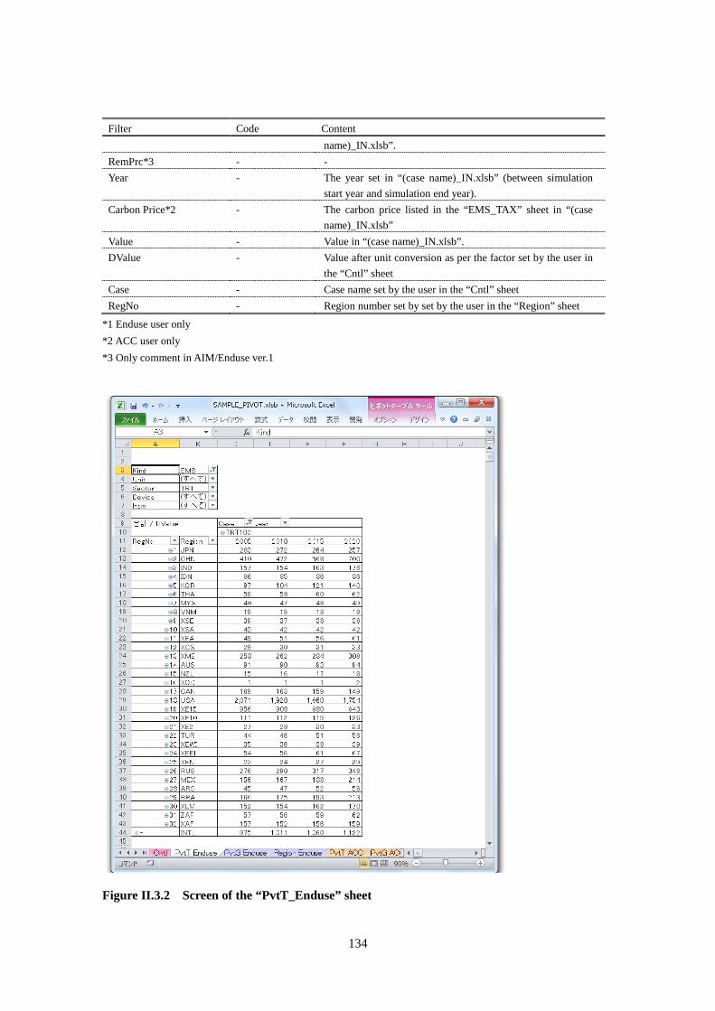
134

Filter Code Content name)_IN.xlsb”.

RemPrc*3 - - Year - The year set in “(case name)_IN.xlsb” (between simulation

start year and simulation end year). Carbon Price*2 - The carbon price listed in the “EMS_TAX” sheet in “(case

name)_IN.xlsb” Value - Value in “(case name)_IN.xlsb”. DValue - Value after unit conversion as per the factor set by the user in

the “Cntl” sheet Case - Case name set by the user in the “Cntl” sheet RegNo - Region number set by set by the user in the “Region” sheet

*1 Enduse user only *2 ACC user only *3 Only comment in AIM/Enduse ver.1

Figure II.3.2 Screen of the “PvtT_Enduse” sheet

135

User can freely change the layout of the pivot table in the “PvtT_Enduse” sheet. If value accidentally

disappears, then open “PivotTable Field List” (Right-click a cell in the pivot table, and in the pop-up

menu, click PivotTable Field List) and check “DValue”. Similarly, if you wish to add/display any

other field (or if it has accidentally disappeared) then check that field in “PivotTable Field List”.

User place a particular field in any of the display sections – Report Filter, Column Labels, Row

Labels, Values – as per the desired format of report.

Figure II.3.3 Screen of the PivotTable Field List

136

2) PvtG: Pivot graph sheet

After finishing data entry in the “Cntl” sheet, click the “Run” button. If the run finishes successfully,

the pivot graph as shown in Figure II.3.4 (“PvtG_Enduse” for AIM/Enduse model; “PvtG_ACC” for

AIM/Enduse[ACC] model) is refreshed automatically.

Figure II.3.4 Screen of the “PvtG_Enduse” sheet

137

3) Region: Region numbering sheet(Optional)

The “Region” sheet as shown Figure II.3.5 (“Region_Enduse” for AIM/Enduse model;

“Region_ACC” for AIM/Enduse[ACC] model) specifies the order of each region. It is optional. The

setting provided in the “Region” sheet is reflected both in “PvtT” and “PvtG” sheets.

Table II.3.5 List of columns in “Region”


NO Integer Number of the region. It is an independent number.

CODE Character The region code listed in the “Region” sheet in “(file name) _IN.xlsb”. Every

code should be unique in the list. If a region name derived from “(case

name)_detail.csv” is not listed in the “Region” sheet, the corresponding

“RegNo” shows “-“ in the “PvtT” sheet.

NAME Character Name of the region. It is optional and not used in calculation.

Figure II.3.5 Screen of the “Region_Enduse” sheet

138

II.4 Description of “(file name)_ACC.xlsb”

II.4.1 Overview

“(file name)_ACC.xlsb” is the user interface to design abatement cost curve (ACC) for a user of

AIM/Enduse[ACC] model. Microsoft Excel2007 is the desirable operating environment (note: the

user whose operating environment is Excel 2003 should use “(file_name)_ACC.xls” in “Excel

2003”).

The process of use of “(file name)_ACC.xlsb” is as follows:

1) Open (file name)_ACC.xlsb (ex. SAMPLE_ACC.xlsb). Any file name and file location can be

set by a user.

2) Enter the data in the “Cntl” sheet. The sheets “ACT” and “ACG” are automatically refreshed

after executing “Run” in the “Cntl” sheet. The “Observed” sheet is necessary when the user

choses option 3 for analysis in the “Cntl” sheet, i.e. with X-axis as “Reduction rate vs the year”.

This is explained later.

3) After finishing data entry, please select “Run”. If execution finishes successfully, the program

opens the “ACG” sheet.

139

II.4.2 Control sheet

“(File name)_ACC.xlsb“ loads “(case name)_detail.csv” and displays the abatement cost curve by

executing Excel/VBA. The “Cntl” sheet as shown in Figure II.4.1 appears on opening the file “(file

name)_ACC.xlsb“.


140

The items in the “Cntl” sheet are listed in the following tables.

Table II.4.1 Items in a “Cntl” related to X-axis (upper level)


CK Three choices Select “1” when X-axis is reduction quantity.

Select “2” when X-axis is reduction rate vs B.L. case.

Select “3” when X-axis is reduction rate vs the year.

-Setting minimum scale of y-axis of MACG (graph). If you want

to set 0 for a minimum scale, select “0” in the list.

NO - -

X-axis - -

Ref Year Integer Enter the value when option “3” is selected in CK.

Ref Sheet Character Enter the value (sheet name) when option “3” is selected in CK.

MinValue For Y-axis Single This spesifies the minimum value for Y-axis of the abatement

cost curve in the “ACG” sheet.

Table II.4.2 Items in a “Cntl” related to Unit Setting (middle level)


CK *(asterisk) If you leave this blank, the unit setting specified in the

corresponding row is used for calculation/display of results.

Check *(asterisk) to the row which you want to exclude in the

results calculation/display.

NO - -

Item - -

Scale Single Factor for the unit conversion. It is used for unit conversion

between original unit and displayed unit in the output results.

CSV Unit Character Original unit.

Display Unit Character Display unit.

141

Table II.4.3 Items in a “Cntl” related to File location (bottom level)


CK *(asterisk) If you leave this blank, simulation results corresponding this row’s

setting are imported from “(case name)_detail.csv”. Check

*(asterisk) to a row if you want to exclude the correspondng results

in diaplay sheets.

NO Integer Number of the row. It is an independent number and is not used in

calculation.

Region Character Region code. The code should be listed in the “Region” sheet in

“(case name)_IN.xlsb”. Use “=” and “+” when you select a

combination of two or more regions.

-Left side code of “=” must be single, unique, and different from the

codes used in the result files.

-Right side code of “=” must be used in the result files, between the

code must be linked with “+”.

Sector (All available) Character Sector code. The code should be listed in the “Sector” sheet in “(case

name)_IN.xlsb”. Use “=” and “+” when you select a combination of

two or more sectors.





Gas (All available) Character Gas code. The code should be listed in the “Gas” sheet in “(case

name)_IN.xlsb”. Use “=” and “+” when you select a combination of

two or more gases.





Year Integer Corresponding simulation end year that user entered in the “Cntl”

sheet in “(case name)_IN.xlsb”. This column is automatically filled

after execution.

C.P. Single Corresponding emission tax pattern (carbon price pattern) that user

entered in the “Cntl” sheet in “(case name)_IN.xlsb”. This column is

automatically filled after execution.

File Character Location of file “(case name)_detail.csv”. Click the left cell (blue

colored) to find a file you want to import.

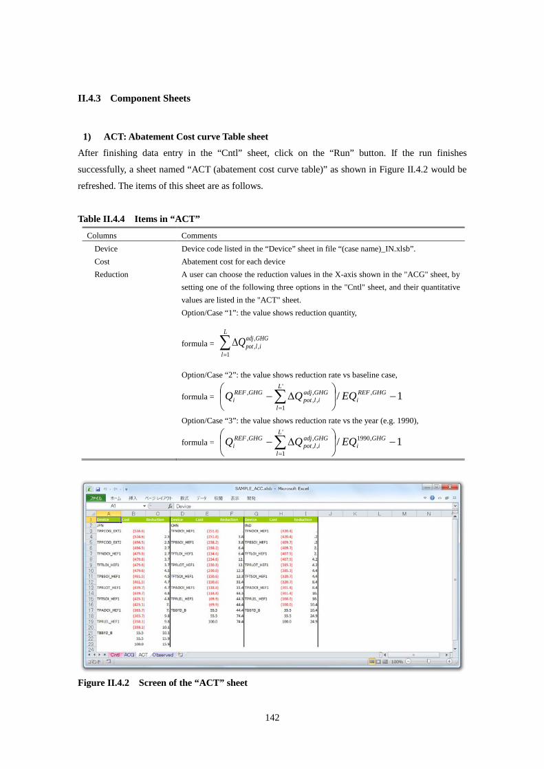
142

II.4.3 Component Sheets

1) ACT: Abatement Cost curve Table sheet

After finishing data entry in the “Cntl” sheet, click on the “Run” button. If the run finishes

successfully, a sheet named “ACT (abatement cost curve table)” as shown in Figure II.4.2 would be

refreshed. The items of this sheet are as follows.

Table II.4.4 Items in “ACT”

Columns Comments Device Device code listed in the “Device” sheet in file “(case name)_IN.xlsb”. Cost Abatement cost for each device Reduction A user can choose the reduction values in the X-axis shown in the "ACG" sheet, by

setting one of the following three options in the "Cntl" sheet, and their quantitative values are listed in the "ACT" sheet. Option/Case “1”: the value shows reduction quantity,

formula = ∑=

∆L

l

GHGadjilpotQ

1

,,,

Option/Case “2”: the value shows reduction rate vs baseline case,

formula = 1/ ,'

1

,,,

, −

∆−∑

=

GHGREFi

L

l

GHGadjilpot

GHGREFi EQQQ

Option/Case “3”: the value shows reduction rate vs the year (e.g. 1990),

formula = 1/ ,1990'

1

,,,

, −

∆−∑

=

GHGi

L

l

GHGadjilpot

GHGREFi EQQQ

Figure II.4.2 Screen of the “ACT” sheet

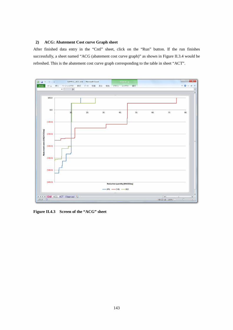
143

2) ACG: Abatement Cost curve Graph sheet

After finished data entry in the “Cntl” sheet, click on the “Run” button. If the run finishes

successfully, a sheet named “ACG (abatement cost curve graph)” as shown in Figure II.3.4 would be

refreshed. This is the abatement cost curve graph corresponding to the table in sheet “ACT”.

Figure II.4.3 Screen of the “ACG” sheet

144

3) Observed: Observed gas emission sheet (Optional)

The sheet as shown in Figure II.4.4 specifies the observed gas emission in the selected year. When a

user selects option “3” as X-axis in the “Cntl” sheet, it is for the purpose of reporting emission

reduction relative to emission level in the selected year. In this case the observed emission in

selected year must be specified in this sheet. Any sheet name (e.g. “Observed”) can be selected by a

user, but the same name should be used as the name of “Ref Sheet” in the “Cntl” sheet. Items of this

sheet are listed as below.

Table II.4.5 Items in the observed gas emission sheet


CK *(asterisk) If you leave this blank, corresponding row’s data is considered in

calculation. Check *(asterisk) to a row if you want to exclude the

corresponding data from calculation/reporting.

NO Integer Number of the data sets. It is an independent number and is not used in

calculation.

REGION* Character Region code. The code should be listed in the “Cntl” sheet.

SECTOR* Character Sector code. The code should be listed in the “Cntl” sheet.

GAS* Character Gas code. The code should be listed in the “Cntl” sheet.

YEAR* Integer The selected year with which the user wants to compare the emissions.

QNT.* Single Observed gas emission in the selected year.

TYPE Character Explanation of the gas. It is an independent number and is not used in

calculation.

UNIT Character Gas emission unit. It is an independent number and is not used in

calculation.

Reference Character Data source of the value. Publications, bookmarks, etc. It is an

independent number and is not used in calculation.

(Note)* Required field for all users.

145

Figure II.4.4 Screen of the “Observed” sheet

AIM

National Institute for Environmental Studies

http://www-iam.nies.go.jp/aim/

Integrated Model - 国立環境研究所 · 2018-09-05 · AIM Enduse Model Manual . AIM Interim...

Documents

Transcript of Integrated Model - 国立環境研究所 · 2018-09-05 · AIM Enduse Model Manual . AIM Interim...