Integrated Fish-Shellfish Mariculture in Puget Sound - AquaModel
82
Integrated Fish-Shellfish Mariculture in Puget Sound NOAA Award - NA08OAR4170860 Final Report Date of submission: 31 May 2011 Principal Investigator: Jack Rensel Ph. D. 1 Associate Investigators: Kevin Bright 2 , Zach Siegrist 3 1/ Research Scientist Rensel Associates Aquatic Sciences 4209 234th Street N.E. Arlington, WA 98223 2/ Biologist and Institutional Contact American Gold Seafoods LLC (Fish in net pens being crowded for harvest) P.O. Box 669 Anacortes, WA 98221 3/ Aquatic Scientist Rensel Associates Aquatic Sciences 4209 234th Street N.E. Arlington, WA 98223 (mussels being cultured at a mussel raft site)
Transcript of Integrated Fish-Shellfish Mariculture in Puget Sound - AquaModel

Integrated Fish-Shellfish Mariculture in Puget Sound
NOAA Award - NA08OAR4170860
Final Report
Date of submission: 31 May 2011
Principal Investigator: Jack Rensel Ph. D.1
Associate Investigators: Kevin Bright2,
Zach Siegrist3
1/ Research Scientist
Rensel Associates Aquatic Sciences
4209 234th Street N.E.
Arlington, WA 98223
2/ Biologist and Institutional Contact
American Gold Seafoods LLC (Fish in net pens being crowded for harvest)
P.O. Box 669
Anacortes, WA 98221
3/ Aquatic Scientist
Rensel Associates Aquatic Sciences
4209 234th Street N.E.
Arlington, WA 98223
(mussels being cultured at a mussel raft site)
Integrated Fish-Shellfish Aquaculture in Puget Sound, Final Report, May 2011 ii
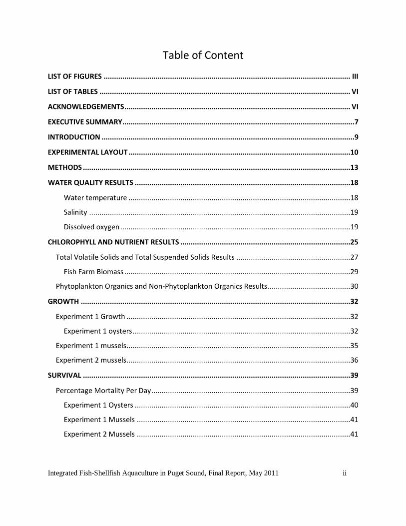
Table of Content
LIST OF FIGURES ....................................................................................................................... III
LIST OF TABLES ......................................................................................................................... VI
ACKNOWLEDGEMENTS ............................................................................................................. VI
EXECUTIVE SUMMARY................................................................................................................7
INTRODUCTION ..........................................................................................................................9
EXPERIMENTAL LAYOUT ...........................................................................................................10
METHODS .................................................................................................................................13
WATER QUALITY RESULTS ........................................................................................................18
Water temperature ...........................................................................................................18
Salinity ..............................................................................................................................19
Dissolved oxygen ...............................................................................................................19
CHLOROPHYLL AND NUTRIENT RESULTS ..................................................................................25
Total Volatile Solids and Total Suspended Solids Results .......................................................27
Fish Farm Biomass .............................................................................................................29
Phytoplankton Organics and Non-Phytoplankton Organics Results........................................30
GROWTH ..................................................................................................................................32
Experiment 1 Growth ............................................................................................................32
Experiment 1 oysters .........................................................................................................32
Experiment 1 mussels............................................................................................................35
Experiment 2 mussels............................................................................................................36
SURVIVAL .................................................................................................................................39
Percentage Mortality Per Day ................................................................................................39
Experiment 1 Oysters ........................................................................................................40
Experiment 1 Mussels .......................................................................................................41
Experiment 2 Mussels .......................................................................................................41

Integrated Fish-Shellfish Aquaculture in Puget Sound, Final Report, May 2011 iii
Size and Timing of Mussel Mortality ......................................................................................42
Summary: Size and Timing of Mussel Mortalities...................................................................44
STABLE ISOTOPE ANALYSES ......................................................................................................45
Stable Isotope Primer ............................................................................................................45
Hypotheses And Approach ....................................................................................................49
Stable Isotope Analyses .........................................................................................................49
Clam Bay ...............................................................................................................................51
Cypress Island .......................................................................................................................53
Mixing Model Analyses..........................................................................................................56
DECISION MATRIX ....................................................................................................................61
FURTHER INTERPRETATION ......................................................................................................63
Oysters ..............................................................................................................................63
Mussels .............................................................................................................................64
Feeding Selectivity and Other Explanations .......................................................................65
Optimum Siting versus IMTA? ...........................................................................................67
The Future for IMTA in Puget Sound and Strait of Juan de Fuca .........................................69
REFERENCES CITED ...................................................................................................................71
APPENDICES .............................................................................................................................74
LIST OF FIGURES
Figure 1. Vicinity map and locations ...........................................................................................9
Figure 2. Google map images of the two study sites at Clam Bay and Cypress Island. ...............12
Figure 3. Diagrams of the experimental layouts at each study site. Treatment and reference
groups represented by blue rectangles. For Clam Bay, flow was tangential through the side of
the cages and the 2D picture does not fully represent the arrays properly. See prior aerial
image for spatial relationships. .................................................................................................13
Figure 4. String of 4 oyster and 4 mussel stocked Aquapurses being placed at the Clam Bay site.
.................................................................................................................................................14

Integrated Fish-Shellfish Aquaculture in Puget Sound, Final Report, May 2011 iv
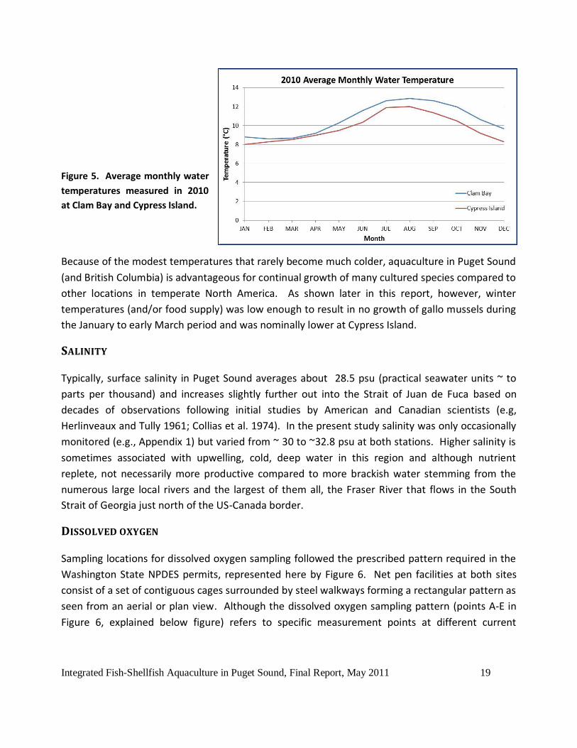
Figure 5. Average monthly water temperatures measured in 2010 at Clam Bay and Cypress
Island. .......................................................................................................................................19
Figure 6. Layout of allowable impact zone around net pens in Washington State and sampling
stations for dissolved oxygen in this project. .............................................................................20
Figure 7. Screen print of AquaModel simulation of oyster rafts. See text for explanation. .......24
Figure 8. Screen print of AquaModel simulation of oyster rafts current velocity of 6 cm/s (0.12
knots) at the same time as above but with the vertical profile point moved 30m downstream. 24
Figure 9. Screen print of AquaModel simulation of oyster rafts current velocity of 1.5 cm/s
(0.03 knots) shortly after the previous time period and with the vertical profile point placed
through the lower left raft location. ..........................................................................................25
Figure 10. Clam Bay and Cypress Island dissolved inorganic nitrogen (DIN) and Chlorophyll a
sampled during Experiment 1. ...................................................................................................26
Figure 11. Clam Bay and Cypress Island monthly total volatile solids (TVS) and total suspended
solids (TSS) at 2 and 20 m depths. .............................................................................................28
Figure 12. Monthly biomass at Clam Bay and Cypress Island Sites from June 2009 to March
2011. Biomass units in metric tons. ...........................................................................................29
Figure 13. Phytoplankton Organics and Non-Phytoplankton Organics for Clam Bay and Cypress
Island, calculated from water quality samples taken between October 2008 and August 2009. 31
Figure 14. Total length increase of Clam Bay mussels and oysters cultured during Experiment 1.
.................................................................................................................................................32
Figure 15. Net length increase of Clam Bay oysters for all three-measurement periods of
Experiment 1. Top panel = first growth period, middle panel = second growth period, bottom
panel = final growth period .......................................................................................................33
Figure 16. Net length increase of Cypress Island oysters during incremental periods of
Experiment 1. ............................................................................................................................34
Figure 17. Cypress Island oyster net length increase during Experiment 1. ...............................35
Figure 18. Clam Bay and Cypress Island mussel net length change September 2008 to June
2009. .........................................................................................................................................36

Integrated Fish-Shellfish Aquaculture in Puget Sound, Final Report, May 2011 v
Figure 19. Net growth of mussels for the entire culture period during Experiment 2. ...............37
Figure 20. Incremental net increases in length of mussels at Clam Bay (left) and Cypress Island
(right) during the algal growing season and fall-winter season. .................................................38
Figure 21. Total mussel growth measured during Experiment 2, including measured mussel
lengths at beginning of experiment. ..........................................................................................39
Figure 22. Percentage of total mortalities per day for Experiment 1 and Experiment 2. ...........40
Figure 23. Total mussel mortalities and percent total mussel mortalities per day for Experiment
2................................................................................................................................................42
Figure 24. Observed average mussel mortality lengths and SD in Experiment 2........................43
Figure 25. Comparison of live mussel lengths and mortality average lengths and SD. ...............44
Figure 26. Cartoon of heavy 13Carbon with one more proton than light 12Carbon isotope, with
red circle representing neutron mass of each and the teeter totter illustrating the relative
weights (after Fry 2006, but drawn from scratch). .....................................................................46
Figure 27. Nitrogen and Carbon stable isotope signatures of various food sources, wastes and
initially stocked mussels for Experiments 1 and 2 combined. Seston pictured here is Clam Bay
seston. ......................................................................................................................................50
Figure 28. Clam Bay (CB) oyster carbon and nitrogen stable isotope results for January (mid
experiment) and June (experiment end) 2009 in Experiment 1, compared to initial values. ......51
Figure 29. Clam Bay (CB) mussel C and N stable isotope Experiment 1 results, January and June
2009, compared to initial values. ..............................................................................................52
Figure 30. Clam Bay (CB) mussel C and N stable isotope Experiment 2 results, September 2010
and March 2011, compared to initial values. .............................................................................53
Figure 31. Cypress Island oyster stable isotope results for January (mid experiment) and June
(experiment end) 2009 in Experiment 1. ...................................................................................54
Figure 32. Cypress Island mussel C and N stable isotope Experiment 1 results, January and June
2009, compared to initial values. ..............................................................................................55

Integrated Fish-Shellfish Aquaculture in Puget Sound, Final Report, May 2011 vi
Figure 33. Cypress Island (CI) mussel C and N stable isotope Experiment 2 results, September
2010 and March 2011, compared to initial values. ....................................................................55
Figure 34. IsoSource mixing model probability distribution histograms for Cypress Island
oysters. .....................................................................................................................................58
Figure 35. Dual isotope plot of Cypress Island oysters and their food sources. Fish feces data
has a standard deviation of ±0.12 Nitrogen and ±0.3 Carbon; phytoplankton standard deviation
is unknown. ...............................................................................................................................60
LIST OF TABLES
Table 1. Sampling design spatial layout of Experiment 1 (September 2008 – June 2009) and
Experiment 2 (April 2010 – 10 March 2011). Depth in meters to the center of each string of
Aquapurses. ..............................................................................................................................11
Table 2. Results of dissolved oxygen monitoring at sampling stations around Cypress Island
(Site 1) and Clam Bay net pens with reference minus mean pen values plus grand average
difference shown in right column. Ref. = Reference location. From Rensel 2010. ....................21
Table 3. Food source isotopic values and shellfish isotopic values used in IsoSource. Shellfish
values have been corrected for marine mussel only trophic level jumps (0.5 Carbon and 1.7
Nitrogen were subtracted from their original values). ...............................................................57
Table 4. Mean percentages of each food source consumed by Cypress Island oysters, derived
from IsoSource mixing model data for both treatments and sampling time period, January = Fall
and early winter, June = Winter and Spring. ..............................................................................59
Table 5. Decision matrix that differentiates between significant and non-significant results. ...62
ACKNOWLEDGEMENTS
The main author and coauthor K. Bright also wish to thank Taylor Shellfish for providing Aquapurse rearing enclosures, seed stock and assistance in field work. Assistance from managers and staff at both net pen sites was also critical in performing this study. The project was supported in part by an award from a competitive grant from the National Oceanic and Atmospheric Administration, number NA08OAR4170860. This report should be cited as: Rensel, J.E., K. Bright and Z. Siegrist. 2011. Integrated fish-shellfish mariculture in Puget Sound. NOAA Award – NA080AR4170860. NOAA National Marine Aquaculture Initiative. Rensel Associates, Arlington Washington in association with American Gold Seafoods and Taylor Shellfish. 82 p.

Integrated Fish-Shellfish Aquaculture in Puget Sound, Final Report, May 2011 7
EXECUTIVE SUMMARY
We evaluated the efficacy of waste transfer from Atlantic salmon aquaculture pens to shellfish
cultured immediately downstream and at different depths and distances in Puget Sound,
Washington. Studies occurred concurrently in central Puget Sound near Clam Bay and in north
Puget Sound at Cypress Island. Fish have been cultivated continuously since 1969 at the former
site and since 1980 at the latter site. Both of these areas are moderately enriched with nutrients
and phytoplankton due to the naturally occurring upwelling of nutrient-rich deep-water along the
west coast U.S.
The null hypothesis for this work was that growth of shellfish would not be enhanced or tracing of
stable isotopes of carbon and nitrogen would not show spatial effect of being near the fish farm.
The alternative hypothesis was that one or both would demonstrate an effect. We suspended
Pacific oysters (Crassostrea gigas) and “gallo” mussels (Mytilus galloprovincialis) in plastic
Aquapurse culture units at several sites at varying distances and depths relative to fish farm net
pens for about 9 months (fall to spring) in Experiment one and for mussels only in Experiment two
for April through March of the following year. As fish farms in this region are dependent on tidal
currents to supply oxygen to the cages, we placed several treatments of shellfish below the
surface layer to assess their growth at strata that would not interfere with surface currents. Prior
studies have shown these areas to be well vertically mixed, so we hypothesized and indeed
confirmed that there was no measureable difference between near surface and subsurface
concentrations of phytoplankton measured as chlorophyll a.
Oysters at Cypress Island received significant nutritional and growth benefits from placement near
the salmon net pens. Oysters closer to the net pens experienced consistently higher growth and
were able to take advantage of fish feces produced by the site. Increased oyster growth nearer
the Clam Bay net pens was measured in the first fall and early winter, but by the completion of
grow out in spring, there were statistical differences among treatments and no evidence of a
stable isotope signature in the tissue of the oysters indicative of fish farm wastes. Comparison of
TVS, TSS, phytoplankton organics, non-phytoplankton organics, chlorophyll a and seston stable
isotope data collected concurrently do not fully explain the differences between growth and
stable isotope signatures at the two sites. No significant differences in these water quality
parameters were noted up or downstream of the fish farms or at different depths. Sampling was
conducted at random times, and had we sampled during feeding would undoubtedly have
measured greater concentrations of TSS and TVS downstream. Lack of differences among sites
could be due to fast changing phytoplankton and seston composition over time scales of days to
weeks, where our sampling for these factors was through economic necessity, monthly.
Integrated Fish-Shellfish Aquaculture in Puget Sound, Final Report, May 2011 8
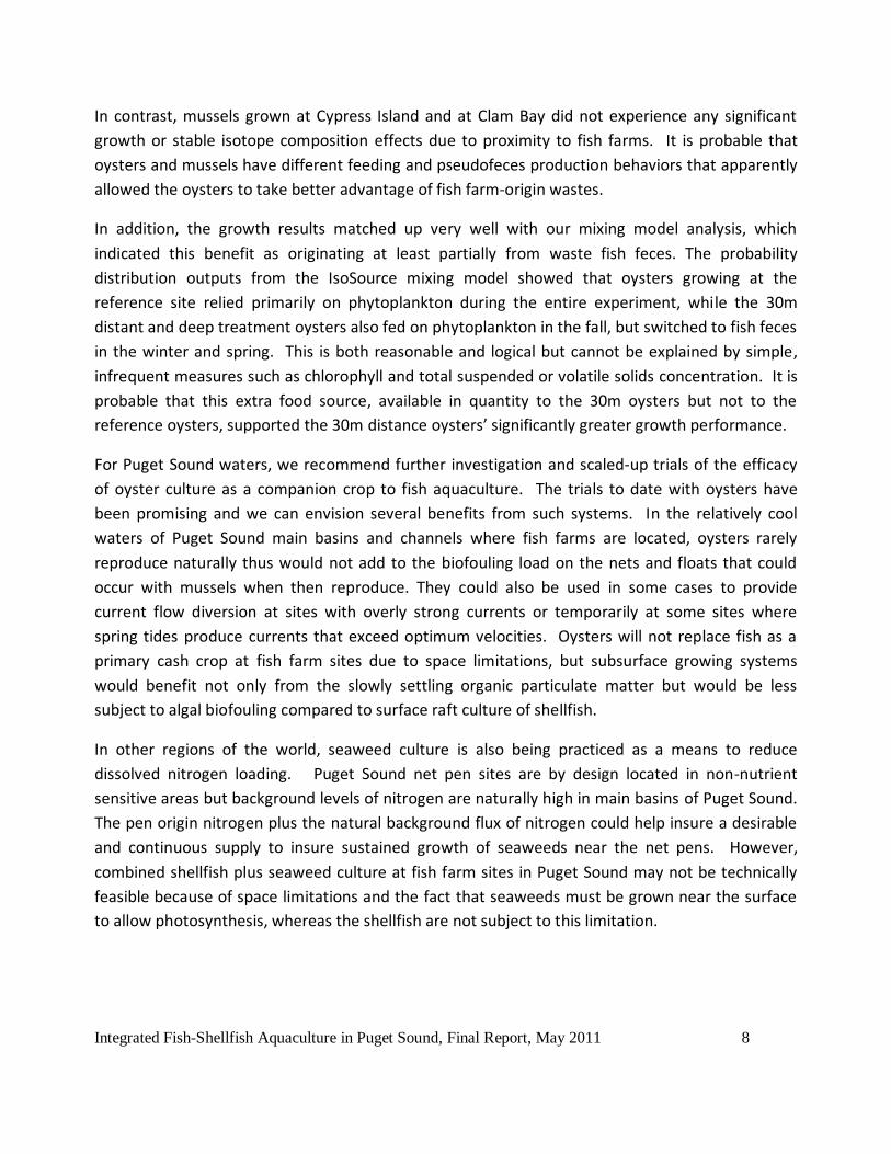
In contrast, mussels grown at Cypress Island and at Clam Bay did not experience any significant
growth or stable isotope composition effects due to proximity to fish farms. It is probable that
oysters and mussels have different feeding and pseudofeces production behaviors that apparently
allowed the oysters to take better advantage of fish farm-origin wastes.
In addition, the growth results matched up very well with our mixing model analysis, which
indicated this benefit as originating at least partially from waste fish feces. The probability
distribution outputs from the IsoSource mixing model showed that oysters growing at the
reference site relied primarily on phytoplankton during the entire experiment, while the 30m
distant and deep treatment oysters also fed on phytoplankton in the fall, but switched to fish feces
in the winter and spring. This is both reasonable and logical but cannot be explained by simple,
infrequent measures such as chlorophyll and total suspended or volatile solids concentration. It is
probable that this extra food source, available in quantity to the 30m oysters but not to the
reference oysters, supported the 30m distance oysters’ significantly greater growth performance.
For Puget Sound waters, we recommend further investigation and scaled-up trials of the efficacy
of oyster culture as a companion crop to fish aquaculture. The trials to date with oysters have
been promising and we can envision several benefits from such systems. In the relatively cool
waters of Puget Sound main basins and channels where fish farms are located, oysters rarely
reproduce naturally thus would not add to the biofouling load on the nets and floats that could
occur with mussels when then reproduce. They could also be used in some cases to provide
current flow diversion at sites with overly strong currents or temporarily at some sites where
spring tides produce currents that exceed optimum velocities. Oysters will not replace fish as a
primary cash crop at fish farm sites due to space limitations, but subsurface growing systems
would benefit not only from the slowly settling organic particulate matter but would be less
subject to algal biofouling compared to surface raft culture of shellfish.
In other regions of the world, seaweed culture is also being practiced as a means to reduce
dissolved nitrogen loading. Puget Sound net pen sites are by design located in non-nutrient
sensitive areas but background levels of nitrogen are naturally high in main basins of Puget Sound.
The pen origin nitrogen plus the natural background flux of nitrogen could help insure a desirable
and continuous supply to insure sustained growth of seaweeds near the net pens. However,
combined shellfish plus seaweed culture at fish farm sites in Puget Sound may not be technically
feasible because of space limitations and the fact that seaweeds must be grown near the surface
to allow photosynthesis, whereas the shellfish are not subject to this limitation.

Integrated Fish-Shellfish Aquaculture in Puget Sound, Final Report, May 2011 9
INTRODUCTION
The purpose of this study was to assess the use of integrated multitrophic aquaculture (IMTA)
using coupled fish and shellfish aquaculture in differing regions of Puget Sound, Washington where
existing net pen salmon aquaculture occurs. IMTA offers a possibility to capture valuable organic
wastes from fish farms to be incorporated into “companion crops” to help diversify production
and reduce organic waste loading in the vicinity of the culture area. The hypothesis for this work is
that growth of shellfish will be enhanced or stable isotope tracing of carbon and possibly nitrogen
will show an effect. The alternative hypothesis is that no growth or stable isotope effect will
occur.
We selected Pacific oysters (Crassostrea gigas) and “gallo” mussels (Mytilus galloprovincialis) as
our target shellfish species. Pacific oysters are a hearty species and grow well throughout Puget
Sound and gallo mussels generally grow better than native mussels (Mytilus trossulus) in areas like
Southern Puget Sound and near Whidbey Island in Saratoga Passage, and were available as seed
stock from local hatcheries. The salmon farms
culture Atlantic salmon (Salmo salar) as there is
a high demand for the species and very low or
no risk of escaped Atlantic salmon colonizing or
establishing populations in the Pacific
Northwest in the studied opinion of experts at
the National Oceanic and Atmospheric
Administration (e.g., Nash and Waknitz 2003).
This research took place at two net pen sites in
Puget Sound, Clam Bay in central Puget Sound
and Cypress Island Site 3 in North Puget Sound
(Figure 1). These sites have differing
hydrographic characteristics and seasonal
differences but both experience moderately
abundant phytoplankton density during the
growing season and modest occurrence of
seston.
Figure 1. Vicinity map and locations

Integrated Fish-Shellfish Aquaculture in Puget Sound, Final Report, May 2011 10
Two experiments were conducted: Experiment 1 commenced in fall and was designed to assess
efficacy of IMTA during winter, the period of lowest phytoplankton abundance for both oysters
and mussels. Experiment 2 began in late spring and ended in early spring to assess different
culture period results for mussels, and to further investigate the results of Experiment 1 with
mussels only.
Water temperatures are moderate in Puget Sound and adjacent marine waters compared to
Northeast United States coastal areas and there are no problems with sea lice infection due to the
prevalence of lower salinity water than in many other salmon farming areas of the world. As
explained in this report, however, coastal and local upwelling of deep oceanic water that is low in
dissolved oxygen does occur in late spring through fall in some areas and years, so placement of
shellfish upstream of current flows would have to be carefully considered with regard to further
interference with oxygen supply as explained in the next section of this report.
EXPERIMENTAL LAYOUT
Location of stations for culture of the shellfish was based on knowledge of persistent tidal current
velocity and direction at both sites. Data sources for Clam Bay were dual recording current meter
records of Weston and Gowen (unpublished, cited in WDF 1990) and for Cypress Island the current
meter results of Rensel (1996) plus local knowledge of the fish farming staff were used in this
regard.
Table 1 summarizes the layout of treatments for Experiments 1 and 2. In each experiment, four
spatial pattern treatments were established: two treatments were placed adjacent to the net
pens, one at a shallow depth and one deeper but both within 1 horizontal meter and downstream
of active salmon pens. Another treatment was placed an intermediate distance (30 meters) away
from the pens, at much greater depth to intercept sinking particulate waste matter. A fourth
treatment was placed approximately 150 m from the pens at a deeper depth. The two treatments
closest to the net pens are referred to as “farm shallow” and “farm deep,” the intermediate
distance treatment is called the “30m distant deep” treatment, and the farthest treatment is
referred to as “reference deep”.

Integrated Fish-Shellfish Aquaculture in Puget Sound, Final Report, May 2011 11
Table 1. Sampling design spatial layout of Experiment 1 (September 2008 – June 2009) and
Experiment 2 (April 2010 – 10 March 2011). Depth in meters to the center of each string of
Aquapurses.
Study Area Treatment
Site
Experiment 1
Depth (m)
Experiment 2
Depth (m) Distance from cages
Cypress Island,
North Puget Sound
Farm
shallow 5 5 Immediately adjacent to cage array,
east end
Same Farm deep 20 15 Immediately adjacent to cage array,
east end
Same 30m
distant
deep
10 15 30 m from above strings
Same Reference
deep 10 15 Reference area 200 m from nearest
pens but in same bay
Clam Bay,
Central Puget Sound
Farm
shallow 5 10 Immediately adjacent to cage array,
South side
Same Farm deep 25 25 Immediately adjacent to cage array,
South side
Same 30m
distant
deep
15 25 30 m further south of pens and above
arrays
Same Reference
deep 15 25 150 m ESE of pens ESE in same bay
Experiment 1: 03 September 2008 – 10 June 2009 at Clam Bay; 05 September 2008 – 12 June 2009 at Cypress Island
Experiment 2: 13 April 2010 – 10 March 2011 at Clam Bay; 14 April 2010 – 11 March 2011 at Cypress Island
The emphasis on deep treatments relates to the need to grow shellfish in a manner that would not
interfere with currents and oxygen flux into the pens. Since these sites are relatively well mixed
without significant vertical stratification at any time of year, it was hypothesized that sufficient
plankton would be available as feed at depth and that much of the particulate waste stream from
the cages could be intercepted at such depths. Figure 2 shows aerial photo images with the
stations superimposed at each site.
When designing Experiment 2, treatment depths were slightly changed for Clam Bay, but kept the
same for Cypress Island. The Clam Bay farm shallow treatment depth was increased from 5 to 10
meters, and the 30m distant deep and reference group depths were increased from 15 to 25

Integrated Fish-Shellfish Aquaculture in Puget Sound, Final Report, May 2011 12
meters. The farm deep treatment was kept the same, at 25 meters deep. These changes were
made because the Clam Bay site is significantly deeper in general than the Cypress Island site and
we wished to further assess shellfish culture at these depths. A diagram of the treatment and
reference locations relative to each site is shown in Figure 3. Because depth at the selected
Deepwater Bay site was shallower than the Clam Bay site, only one depth was used for each of the
three strings of deep shellfish cages. At Clam Bay, a deep set of cages was installed beneath the
set that was adjacent to the pens. Waste fecal matter of salmonids, particularly larger ongrowing
fish, sinks relatively rapidly and it was thought that we may see a difference among the shallower
and deeper strings.
Figure 2. Google map images of the two study sites at Clam Bay and Cypress Island.
The other net pen shown in Figure 2 at Cypress Island was not occupied during these experiments.
Current velocity at the Cypress Island site averaged about 15.5 cm/s during current meter
monitoring of a mean tidal exchange day at this site (Rensel 1996). Currents were strongly
bidirectional with the ebb tide flowing through the pens from west to east into the location of the
IMTA trial Aquapurse units. No current meter information was available from the Clam Bay site
but judging from the coarse sand bottom and large carrying capacity of the site that routinely
meets NPDES performance standards, currents are equally as strong on average. Previously,
Weston and Gowen (unpublished, cited in WDF 1990) had a recording of Aanderaa Vane style
EBB
Clam Bay
Cypress Island

Integrated Fish-Shellfish Aquaculture in Puget Sound, Final Report, May 2011 13
current meters on both ends of this site, but that location was slightly shallower than the present
day site location.
Figure 3. Diagrams of the experimental layouts at each study site. Treatment and reference groups
represented by blue rectangles. For Clam Bay, flow was tangential through the side of the cages and the
2D picture does not fully represent the arrays properly. See prior aerial image for spatial relationships.
METHODS
Juvenile shellfish used in both experiments were produced by Taylor shellfish and originated in
Southern Puget Sound. Experiment 1 used both Crassostrea gigas (triploid Pacific oysters) and
Mytilus galloprovincialis (blue mussels) while Experiment 2 only used M. galloprovincialis. For
both experiments, mussels were hatched in Dabob Bay and oysters in Quilcene Bay. They were
later moved to nearby nursery grounds: Totten Inlet for the mussels, Oakland Bay for the oysters.
At the beginning of Experiment 1, shellfish were approximately 10 months old at time of stocking;
juvenile mussels used in Experiment 2 were younger (7 months).
All shellfish were cultured in replicate Aquapurse trays (Figure 4), reusable plastic purses that were
set in between perimeter lines with spreader bars at the top and bottom. The strings were set at

Integrated Fish-Shellfish Aquaculture in Puget Sound, Final Report, May 2011 14
different depths and locations as specified in Table 1. At both sites, the net pens are galvanized
steel cage systems with all rearing pens held within the same array. The cages move very little
during tidal cycles, but there is some slight shifting according to GPS measurements made during
routine permit compliance monitoring. In both cases, the immediate downstream Aquapurse
trays were placed in one of two dominant tidal current directions. A commercial project for
mussels would use suspended strings of mussels, but the Aquapurses offered the advantage of
predator avoidance without the use of predator deterrent nets and ease of sampling access.
Figure 4. String of 4 oyster and 4 mussel
stocked Aquapurses being placed at the Clam
Bay site.
On each scheduled sampling date, Aquapurse units were removed from the water and all shellfish
lengths were measured. Length was recorded in millimeters using specialized metric rulers; in the
case of broken shells, length was visually estimated. Shellfish tissue volume was not measured.
Total count of all living specimens and empty shells was also tallied, and lengths of all empty shells
were also measured and recorded in Experiment 2. In addition, during each measurement period,
several shellfish from each Aquapurse were selected at random and removed for later stable
isotope analysis. After all shellfish length measurement was completed, shellfish were placed back
into their respective Aquapurses, which were then re-suspended in the water.

Integrated Fish-Shellfish Aquaculture in Puget Sound, Final Report, May 2011 15
Shellfish mortalities were calculated by subtracting the total amount of live specimens found
during each collection date from the number of live specimens found during the previous
collection date. For example, if there were 50 live mussels measured in September 2010, and 30
in March 2011, there would be 20 mortalities recorded for the September-March period. This was
deemed a more accurate method than simply recording the number of dead specimens and empty
shells found at each collection date, because often-empty shells may break up or otherwise
disappear for a variety of reasons. Percentage of total mortalities per day was also calculated in
order to observe any differences of mortality rate at different sites or treatments. To determine
percentage of total mortalities per day, percentage of total mortality was first calculated for each
measurement period (e.g., April-September and September-March, for Experiment 2, and then
divided by the amount of days of each measurement period.
Experiment 1 also involved collection of a variety of other water quality data, including dissolved
inorganic nitrogen (DIN), chlorophyll a, total volatile solids (TVS) and total suspended solids (TSS).
These were sampled at different depths (2m and 20m), at upstream and downstream locations,
and at different times during the year in order to develop a more complete representation of site
conditions at Clam Bay and Cypress Island. Vertical profile measurements of salinity, temperature,
in vivo chlorophyll a, dissolved oxygen, pH and turbidity have also been collected periodically at
both study sites. These data were collected on some shellfish sampling dates, as well as in
between those periods. Water temperature data and fish farm biomass was also obtained from
the fish farms’ records. In addition, seston and phytoplankton analysis were conducted
periodically at the IMTA sites by analyzing TVS, TSS and chlorophyll a content of the water as
described below, some of which uses calculations based on Hawkins et al. (2002). Analysis of
nutrients was performed by the University of Washington Oceanography Routine Chemistry
Laboratory using state of the art autoanalyzer techniques. TSS, TVS and chlorophyll analyses were
conducted at Aquatic Research Inc. laboratory in Seattle using Washington State Dept. of Ecology
and EPA approved methodologies.
TVS was measured as an estimate of particulate organic matter (POM) which in turn is a crude
surrogate for total available shellfish food. TVS was measured by weighing a GF/F filter before and
after suctioning sample water through it and after combusting the filter to calculate the portion
which ignites.
Likewise, TSS was measured as a representation of the total pool of total particulate matter (TPM)
using standard methods of filtering water and drying the filtrate. TSS was measured by filtering a
water sample on a dry, pre-weighed filter, drying the sample/filter and weighing again.

Integrated Fish-Shellfish Aquaculture in Puget Sound, Final Report, May 2011 16
Chlorophyll a (µg/l units) was measured in the field with a CTD probe (Turner Co. SCUFA) and
discrete samples collected in 1 liter bottles and analyzed at a certified laboratory (Aquatic
Research Incorporated, Seattle, WA) using spectrophotometer based methods. Chlorophyll a is a
surrogate measure of phytoplankton abundance that can be factored below into comparable units
when calculating phytoplankton organics. It serves as a measure of food for shellfish.
Total particulate matter (TPM) was estimated by analysis of total suspended solids (TSS) in mg/L.
Particulate inorganic matter (PIM) was estimated by subtraction of chlorophyll a minus POM.
Phytoplankton organics (abbreviated PHYORG in units of mg/l) was estimated by the method of
Grant and Bacher (1998), where measured chlorophyll a concentration (mg/l) is multiplied by the
coefficient value 50 (for relatively rich growing waters such as Puget Sound, see Welschmeyer and
Lorenzen (1984) and Taylor et al. (1997)). This is the so-called carbon to chlorophyll a ratio and
varies considerably. That value of total phytoplankton organic carbon is then divided by the factor
of 0.38 (a conversion factor for algae in nearshore waters) to achieve an estimate of PHYORG.
Non-phytoplankton organics (DETORG in mg/l) was then calculated as POM minus PHYORG. This is
the material not useful for phytoplankton growth (i.e., detritus) although it may be cycled into
phytoplankton through mineralization. Few estimates of PHYORG and DETORG are available for
Puget Sound, although basic POM and related estimates from North Totten Inlet in Southern Puget
Sound have been described in unpublished reports by Brooks (2008). Measured TVS (e.g., POM) of
surface waters of North Totten Inlet averaged 13.5 mg/L (95% CI of +14.6/-12.5) and TSS averaged
51.8 (95% CI of +55.0/-48.5) in this study. South Puget Sound has modest phytoplankton
abundance during the growing season like central and north Puget Sound; however, it is rich in
seston year round compared to these other areas. The actual cause of this situation is unknown,
but circulation with the ocean is restricted and turbidity relatively high compared to the other
basins of Puget Sound.
The above calculations allow insight into the source of diet for the shellfish, which includes a large,
often major portion of the diet due to non-phytoplankton organics. Unfortunately, this varies
from place to place as well as seasonally, so it has to be determined locally. In these calculations,
we must acknowledge that not all phytoplankton is equally useful for shellfish growth, but this
approach is currently considered one of the few reasonable approaches to measure available
shellfish food supply (e.g., Hawkins et al. 2002).
Shellfish removed for stable isotope analysis were packed on ice and brought back to Arlington,
Washington. Within 24 hours, shellfish tissue consisting of entire soft body viscera was removed

Integrated Fish-Shellfish Aquaculture in Puget Sound, Final Report, May 2011 17
and packaged in Whirl-Pak bags, frozen and shipped to the University of Idaho Stable Isotopes
Laboratory for carbon and nitrogen stable isotope analysis. At the laboratory, samples were
preprocessed by homogenizing the tissue in a mortar and pestle in liquid nitrogen before analysis.
An elemental analyzer (NC2500, CE Instruments, Milan, Italy) was used to liberate N2(g) and CO2(g)
from solid samples by flash combustion, and subsequent oxidation and reduction reactions. A gas
chromatographic column in the elemental analyzer separates the two gas species which are
vented to a mass spectrometer (Delta+, ThermoElectron Corp., Bremen, Germany) via a
continuous flow interface (ConFlo II, ThermoElectron Corp., Bremen, Germany) for isotope ratio
analysis. Standardized acetanilide are analyzed every 11 samples for assurance of stability, drift
correction, and elemental mass fractions. Acetanilide working standards were calibrated against
an acetanilide primary standard and reported as a relative ratio to Peedee belemnite (PDB) for
carbon and as a relative ratio to atmospheric nitrogen for nitrogen. The precision of the specific
analysis was calculated from the standard deviation of the four secondary standard replicates.
The mean of the four acetanilide working standards were used to do a 1‐point correction estimate
of %C and %N. For quality control, a tertiary standard was used to verify the quality of the
normalization applied.
Spatial oxygen consumption of Pacific oysters was estimated from Ren et al. (2000) and used to
calibrate model simulations of AquaModel 3D-GIS based aquaculture monitoring software for a
site with characteristics similar to the Cypress Island sites.
All data was reviewed for QAQC concerns and grouped by species and time period for
computation of basic statistics involving ANOVA and Tukey’s post hoc testing. Microsoft Excel and
Statistix statistical analysis software were used to process and analyze data. In addition, the
number of shellfish mortalities per sampling period was calculated by subtracting the total amount
of live specimens found during each collection date from the number of live specimens found
during the previous collection date. This was deemed a more accurate method than simply
recording the number of dead specimens and empty shells found on each collection date, because
often empty shells may break up or otherwise disappear for a variety of reasons.
To evaluate the significance of IMTA in terms of removing fish farm wastes we constructed a
matrix of possible effects including:
1) Growth in treatments near the farm versus the reference areas, noting that increased growth
near the farms should have been higher if food was a limiting factor.
2) Stable isotope effect, in terms of mixing model results.

Integrated Fish-Shellfish Aquaculture in Puget Sound, Final Report, May 2011 18
3) Survival, in terms of significantly higher shellfish survival at treatment versus reference
locations.
Single stable isotope results were also analyzed, but did not correlate well with growth and mixing
model results and were judged less reliable as a suitable index of performance of the IMTA system.
Because fish produce mostly soluble nitrogen wastes but carbon as particulate wastes (and as
respiration) we would have expected a possible single stable isotope result for carbon, not
nitrogen, but that was not what we found as discussed later.
WATER QUALITY RESULTS
A range of water quality measurements were taken over the course of the experiment in order to
provide supplemental information and potential explanations for growth and stable isotope
results. The majority of water quality data, including chlorophyll a, dissolved inorganic nitrogen
(abbreviated DIN, which includes most of the common nitrogen plant nutrients of nitrate, nitrite
and ammonium), total volatile solids (TVS) and total suspended solids (TSS) were only sampled
during Experiment 1 but still gives an idea of environmental conditions present during Experiment
2. Water temperature, another important factor that may well influence shellfish growth, survival
and feeding habits, was recorded daily by the fish farmers and during our routine sampling
sessions for the majority of both experiments.
WATER TEMPERATURE
Between September 2008 and June 2009, the time period of Experiment 1, Cypress Island water
temperature averaged 8.9 °C. At Clam Bay, water temperature was significantly higher, at 9.8 °C.
Likewise, water temperatures in 2010 were significantly lower at Cypress Island than at Clam Bay,
averaging 9.7 °C and 10.6°C, respectively. In addition to having a higher overall water temperature
at Clam Bay, there were also no individual months in which average water temperatures were
higher at Cypress Island. As an example, Figure 5 shows average monthly water temperature in
2010 for both Clam Bay and Cypress Island.
Integrated Fish-Shellfish Aquaculture in Puget Sound, Final Report, May 2011 19
Figure 5. Average monthly water
temperatures measured in 2010
at Clam Bay and Cypress Island.
Because of the modest temperatures that rarely become much colder, aquaculture in Puget Sound
(and British Columbia) is advantageous for continual growth of many cultured species compared to
other locations in temperate North America. As shown later in this report, however, winter
temperatures (and/or food supply) was low enough to result in no growth of gallo mussels during
the January to early March period and was nominally lower at Cypress Island.
SALINITY
Typically, surface salinity in Puget Sound averages about 28.5 psu (practical seawater units ~ to
parts per thousand) and increases slightly further out into the Strait of Juan de Fuca based on
decades of observations following initial studies by American and Canadian scientists (e.g,
Herlinveaux and Tully 1961; Collias et al. 1974). In the present study salinity was only occasionally
monitored (e.g., Appendix 1) but varied from ~ 30 to ~32.8 psu at both stations. Higher salinity is
sometimes associated with upwelling, cold, deep water in this region and although nutrient
replete, not necessarily more productive compared to more brackish water stemming from the
numerous large local rivers and the largest of them all, the Fraser River that flows in the South
Strait of Georgia just north of the US-Canada border.
DISSOLVED OXYGEN
Sampling locations for dissolved oxygen sampling followed the prescribed pattern required in the
Washington State NPDES permits, represented here by Figure 6. Net pen facilities at both sites
consist of a set of contiguous cages surrounded by steel walkways forming a rectangular pattern as
seen from an aerial or plan view. Although the dissolved oxygen sampling pattern (points A-E in
Figure 6, explained below figure) refers to specific measurement points at different current

Integrated Fish-Shellfish Aquaculture in Puget Sound, Final Report, May 2011 20
locations, both Clam Bay and Cypress Island are subject to oscillating tidal flows and the “down
current” end is not in every case strictly defined. Therefore, in Table 2, we present a collection of
dissolved oxygen data taken at various locations around Clam Bay and Cypress Island net pens
from the National Pollutant Discharge Elimination System (NPDES). These data were taken
without regard to time of tide or direction and show no spatial or temporal trends whatsoever, but
were purposely taken during a period of low dissolved oxygen (Rensel 2010).
Figure 6. Layout of allowable
impact zone around net pens
in Washington State and
sampling stations for
dissolved oxygen in this
project.
See below for station
codes.
A) 100’ (~30m) from “down current” (dominant current or suitable sea bottom) end
B) 100’ from seaward end
C) 100’ from “up current” (less dominant current or unsuitable rocky bottom) end
D) 100’ from shoreward end
E) 50’ (~15m) from “down current” end

Integrated Fish-Shellfish Aquaculture in Puget Sound, Final Report, May 2011 21
Table 2. Results of dissolved oxygen monitoring at sampling stations around Cypress Island (Site 1) and
Clam Bay net pens with reference minus mean pen values plus grand average difference shown in right
column. Ref. = Reference location. From Rensel 2010.
Site & Water
Temp.
Station Code
Direction and
distance from pens
Dissolved Oxygen mg/L
at three different depths
Mean
Difference
(mg/L)
Pen vs.
Ref.
Difference
Cypress Island
11.1°C
1m
Deep
Mid
Water
1m
Above
Bottom
S1N100 5.20 5.16 5.23
S1S100 5.20 5.20 5.19
S1W100 5.14 5.19 5.00
S1W50 5.12 5.15 5.02
S1E100 5.12 5.22 5.32
Mean 5.16 5.18 5.15 5.16
Ref 200’ East 5.08 5.12 5.11 5.10 0.06
Clam Bay 12.4°C
CBSE100 7.30 6.96 6.91
CBSW100 7.25 7.12 7.18
CBNW100 7.13 7.09 7.08
CBNW50 7.12 7.09 7.04
CBNE100 7.38 7.22 6.82
Mean 7.24 7.10 7.01 7.11
Ref 200’ East 7.25 7.01 6.81 7.02 0.09
In order to quantify dissolved oxygen effects of shellfish farms placed by fish farms, we initially
thought we would have to measure dissolved oxygen consumption at a representative mussel
farm. The senior author is highly experienced at measuring flux rates around fish farms but knew
that such field-based estimates pale in accuracy compared to laboratory and model based results.
Therefore instead, we based our estimates on published Pacific oyster respiration rates of Ren et
al. (2000) to calibrate the 3D-GIS aquaculture simulation software AquaModel by substituting in
oysters for fish (see Rensel et al. 2007, Kiefer et al. 2008, Kiefer et al. 2011 for details of the model
construction and operation). The above cited oyster respiration rates were altered by the dry
weight-wet weight conversion factors found in Ricciardi and Bourget (1998).
We estimated that an average 70mm shell length oyster at harvest is respiring at approximately
0.00896 ml O2/hr. Compared to salmon, which have a much higher basal and active metabolism

Integrated Fish-Shellfish Aquaculture in Puget Sound, Final Report, May 2011 22
or approximately 300 mg O2/kg/hr (wet weigh and for normal activity levels), oysters respire much
less, at 8.27 mg O2/kg/hr (wet weight) or 36 times less per unit weight. We applied that correction
factor to the standing stock of fish in the pens to adjust the standing stock of oysters being tested
during the simulation.
A ua odel evaluates sediment and water column effects of floating a uaculture systems and has
not been fully configured for use with shellfish so here we only used the respiration rate of oysters
at 12 C and in a simulation of twelve each 90 m2 rafts with a total estimated annual production of
84 metric tons. This is small compared to a full sized floating shellfish operation, but reasonably
sized given the relatively narrow downstream plume and cross section of a net pen farm with the
current running through them longitudinally, as often occurs in Puget Sound with the strong
current velocities. The shellfish are being held at 12 meter deep and deeper, not at the surface as
per the approximate depth of many of our treatments in this study.
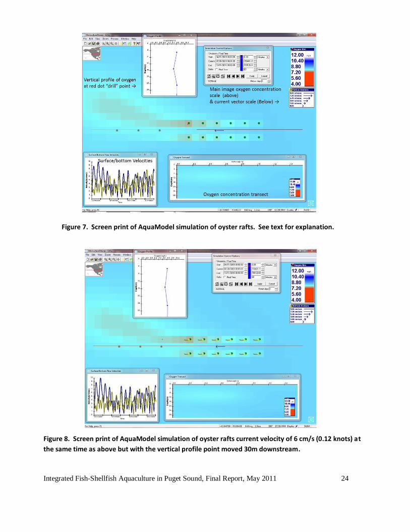
Figure 7 is a screen-print snapshot of one hourly time step in a model run showing the each of the
twelve cages (represented as green dots, not to scale of the outline of the rafts). A vector arrow in
the center of the array indicates (in this case) the near surface current vector (velocity &
direction). The current velocity at this time was a moderate 6 cm/s (0.12 knots) and the oxygen
deficit relative to ambient is shown as a vertical profile taken at the location of the most
northwesterly (reddish) raft and as a small red dot superimposed on that location. Inset charts
show a vertical “drill” profile in the worst-case position (top center/left) and a longitudinal
transect through the cages (bottom right) derived from a moveable red longitudinal line was
drawn through the array to produce a section profile of oxygen in the water column. Surface and
near bottom current velocity is shown as the plot in the lower left. These are but 3 of about 45
different plots available in AquaModel for water column and benthic parameters. Other features
of this plot are the simulation time control that allows the user to play the simulation forwards or
backwards and the main image oxygen concentration scale (upper right) and water current vector
scale (middle right).
In Figure 7 we notice that the oxygen deficit plume is mostly restricted to the water column below
the downstream rafts but is quite small as indicated in the vertical profile and limited to about 0.6
mg/L. Further downstream, by 30 meters distance (first brown dot in a row of three) the
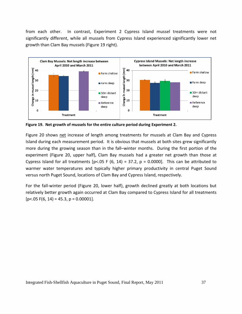
reduction is only 0.3 mg/L less than ambient as shown in Figure 8. The final screen-print of this
series illustrates conditions when flows are near neap, at 3 cm/s and direction of flow has shifted
from north to south as it does at the subject site during the changing of the tidal phase (Figure 9).
This condition represents worst-case oxygen use but of course is restricted to within the culture
area and not being advected downstream any great distance.

Integrated Fish-Shellfish Aquaculture in Puget Sound, Final Report, May 2011 23
We could show many more images at different stages of the tide but the results are generally
similar. For the production unit of this size the dissolved oxygen effect of the oysters is relatively
insignificant compared to what a comparable biomass of fish would produce. This is not to say
that deflection of water flow around the salmon farm from the shielding of the oyster rafts would
not be a problem if the currents were weak, but again, here we are evaluating effects of a
“sunken” oyster raft array.
By way of comparison to real field data, an unpublished study reported by NewFields Northwest
(2008) of shellfish induced oxygen deficit plumes measured around a large mussel farm in Totten
Inlet, South Puget Sound, appeared to affect conditions only a relatively short distance
downstream, often just a few meters downstream. Although the results were variable, in no case
was an effect measurable by 70m away from the mussel rafts. Unfortunately, there were no
measurement locations between a few meters downstream and 70 m downstream. Also for
comparison, Parametrix et al. (1991) reported the results of several dissolved oxygen flux studies
(not just concentrations) at fish farms in Puget Sound that showed no measurable effect
downstream of the farms at a distance of 30 meters. Fish farms were generally smaller then than
they are presently, but given the much greater respiration rates of salmon versus oysters, these
observations show how the modeled estimates may be approximately correct. The 1991 study
was performed by the senior author of this report as a subcontract to Parametrix.
Diversion of water current remains an issue, because it is dissolved oxygen flux – not just
concentrations – that are important to maintain the fish. Fortunately, it appears that at our
selected sites, shellfish grown at 10-15m deep were able to grow at similar rates to surface-
cultured shellfish as discussed later in this report.
Integrated Fish-Shellfish Aquaculture in Puget Sound, Final Report, May 2011 24
Figure 7. Screen print of AquaModel simulation of oyster rafts. See text for explanation.
Figure 8. Screen print of AquaModel simulation of oyster rafts current velocity of 6 cm/s (0.12 knots) at
the same time as above but with the vertical profile point moved 30m downstream.

Integrated Fish-Shellfish Aquaculture in Puget Sound, Final Report, May 2011 25
Figure 9. Screen print of AquaModel simulation of oyster rafts current velocity of 1.5 cm/s (0.03 knots)
shortly after the previous time period and with the vertical profile point placed through the lower left
raft location.
Based on the foregoing, fish farmers in moderate current areas in Puget Sound would have a
choice between 1) placing shellfish at the surface but keeping the density reasonably low; or 2)
placing shellfish subsurface at any desired density that does not invoke a “density dependency”
growth reduction.
CHLOROPHYLL AND NUTRIENT RESULTS
Chlorophyll a and dissolved inorganic nitrogen sampling results are shown below in Figure 10 for
both net-pen sites. Chlorophyll profiles were similar at both upstream and downstream locations
within sites and the general seasonal expected shape was similar, but greater levels of chlorophyll
were observed at Clam Bay in spring and summer. However, since the shellfish were harvested in
June, we note that chlorophyll was somewhat lower on average in Clam Bay versus Cypress Island
during the growth experiment and both sites exhibited low winter values.

Integrated Fish-Shellfish Aquaculture in Puget Sound, Final Report, May 2011 26
Figure 10. Clam Bay and Cypress Island dissolved inorganic nitrogen (DIN) and Chlorophyll a sampled
during Experiment 1.
Increased chlorophyll at Clam Bay in summer is understandable as the bay itself is rapidly flushed
and source waters during the ebb include the Port Orchard (bay) area waters that are often
enriched with phytoplankton due to more ideal algal growing conditions. Source waters for
Cypress Island, really more of bight than a bay, are the relatively open, deep waters of Bellingham
Channel and North Puget Sound.
Fish farms in Puget Sound do not directly affect chlorophyll content of the water as it takes a day
or longer for cells to divide and nutrients are not limiting at farm sites to the growth of
phytoplankton in the main basins of Puget Sound (Rensel Associates and PTI Environmental
Services 1991). Background concentrations of dissolved inorganic nitrogen are naturally high
throughout these areas and note that there was no large or consistent upstream to downstream
nitrogen differences in these measurements. When dissolved nitrogen availability far surpasses
the phytoplankton or seaweed demands in an area, other factors, such as sunlight or vertical
mixing and advection control algal populations. Fish farms produce dissolved nitrogen wastes and
eventually some of that waste is sequestered by phytoplankton or seaweed even if background

Integrated Fish-Shellfish Aquaculture in Puget Sound, Final Report, May 2011 27
concentrations are large. However, the literature clearly demonstrates that other factors,
including sunlight availability and advection of cells to the deep layer are factors considered to
limit primary productivity in the main basins of Puget Sound, and not nutrient supply.
Not shown above in Figure 10 are the 20 m depth DIN results which mirror the 2 m results almost
exactly. This is what is expected in well-mixed or actively mixing areas that represent optimum
fish farm siting. Data tables for all of the above are found in Appendix 2.
TOTAL VOLATILE SOLIDS AND TOTAL SUSPENDED SOLIDS RESULTS
Total volatile solids (TVS) and total suspended solids (TSS) were measured in order to analyze
available shellfish food. TVS can act as an estimate of particulate organic matter (POM) which is a
surrogate for total available shellfish food; TSS represents a measure of the total pool of
particulate matter and can be used in conjunction with other measurements to calculate
phytoplankton organic matter and non-phytoplankton organics.
In Figure 11 we show TVS and TSS results for Clam Bay and Cypress Island. Error bars are not
included as often single samples were collected, although we collected at least one duplicate
sample daily as a quality assessment measure and results indicate that the duplicates in all cases
closely matched the companion sample. We sampled upstream and downstream or the pens, and
compared to see if there was a difference, but t-tests of the data indicate no significant differences
overall. This is a bit surprising, especially for the 20 m depths, as the fish farms have large
amounts of fish biomass on hand (Figure 12).
Immediately apparent in Figure 11 are the seasonal and total variation between sites. Clam Bay
had lower TVS in fall through spring, but higher concentrations in summer than Cypress Island. For
TSS, Clam Bay was consistently lower throughout the year with the exception of the final sample in
August 2009. Just based on these results, we would have expected Deepwater Bay to produce
larger oysters and mussels. However, the opposite occurred, which may be due to the
confounding effect of colder average temperatures at Cypress Island, and/or differences in food
quality. Phytoplankton species composition was not assessed, as funds were limited for this
project. However, routine sampling for harmful algae during the growing season has been
conducted for decades at these sites by the fish farmer technicians who are trained in this matter
and no overtly different species composition differences have been noted between these sites.

Integrated Fish-Shellfish Aquaculture in Puget Sound, Final Report, May 2011 28
Figure 11. Clam Bay and Cypress Island monthly total volatile solids (TVS) and total suspended solids
(TSS) at 2 and 20 m depths.
Sutherland et al. (2001) found an increase in suspended particulate matter (SPM) immediately
next to a salmon net pen in the Broughton Archipelago of British Columbia of 0.6 mg/L but that
was within the middle of the fish cages. Only 30% of that was seen immediately adjacent to the
pens at 5 m distance. About 80% of the inside SPM pen load was measured vertically below the
pens. Sampling was conducted when the tide was running at reasonable strength of 10 cm/s
below the pens (which is sufficient for sea bottom resuspension of wastes). Samples were
collected on a transect up to 30 m from the farm but results were not reported. A reference
station 500 m distant had lower levels of particulate organic matter than within and immediately
adjacent to the farm site. Dr. Sutherland is an experienced worker in the field and no doubt these
measurements were made to the highest level of accuracy. The authors’ measurements were
during feeding periods only and were not put into context of background variation in other
regional areas, and we believe the maximum results (0.6 mg/L) represent a very small effect.
We cannot directly compare results with the Sutherland et al. study as we used TSS rather than
SPM, a somewhat different methodology, but nevertheless another measure of particulate matter

Integrated Fish-Shellfish Aquaculture in Puget Sound, Final Report, May 2011 29
in the water column that should have produced similar results. Our reference samples (not
upstream, but remote upstream) were similar to the upstream samples (Appendix 2). Overall,
both Puget Sound sites had significantly higher particulate matter results(~3 to 8 mg/L) compared
to the B.C. site (maximum of 0.6 mg/L) and we present multiple day results whereas the B.C. study
represented single feeding events (of unknown number) over a three day period in March. We
can say that background levels of particulates are much higher at the Puget Sound sites and that
there was no consistent production of particulate matter measured downstream.
In addition, our measured TSS and TVS values are much lower than those measured by Brooks
(2008); however, Brooks’ data are from southern Puget Sound in North Totten Inlet, which often
experiences much higher TVS and TSS than the waters of northern Puget Sound. Totten Inlet is a
prime oyster and mussel growing area in Puget Sound.
FISH FARM BIOMASS
Fish farm biomass was consistently greater at Clam Bay than at Cypress Island (Figure 12). Clam
Bay operations ranged from approximately 725 to 2300 metric tons; Cypress Island net pens
contained standing stock of between ~400 and 860 metric tons.
Figure 12. Monthly biomass at Clam Bay and Cypress Island Sites from June 2009 to March 2011. Biomass
units in metric tons.

Integrated Fish-Shellfish Aquaculture in Puget Sound, Final Report, May 2011 30
PHYTOPLANKTON ORGANICS AND NON-PHYTOPLANKTON ORGANICS RESULTS
As explained in the methods, phytoplankton organics (abbreviated PHYORG in units of mg/l) and
non-phytoplankton organics (DETORG in mg/l) were calculated using TSS and chlorophyll a data, as
well as several coefficient and conversion factors found in the literature. These calculations allow
insight into the source of diet for the shellfish, which includes a large, often major portion of the
diet due to non-phytoplankton organics. Unfortunately, this varies from place to place as well as
seasonally, so it has to be determined locally. In these calculations, we must acknowledge that not
all phytoplankton is equally useful for shellfish growth, but this approach is currently considered
one of the few reasonable approaches to measure available shellfish food supply (e.g., Hawkins et
al. 2002).
Figure 13 shows calculated PHYORG and DETORG for both Clam Bay and Cypress Island. Similar to
other water quality results, all data are from sampling between October 2008 and August 2009.
Overall, PHYORG at Clam Bay was slightly greater than at Cypress Island, notably during the spring
and summer months. Without exception, non-phytoplankton organics were greater than
phytoplankton organics at both sites. The contrast between DETORG and PHYORG is especially
strong during the winter months, which is supported by the fact that phytoplankton are much
more abundant during the spring and summer. During the winter, shellfish must rely on other diet
sources, which in the present treatment cases may include fish feed and feces. Indeed, this was
supported with our stable isotope mixing results, which are presented later in this report.
To summarize, the most important aspect of this analysis is the consistently higher winter non-
phytoplankton organics at the Cypress Island site (Figure 13 lower right). This result stems from
the also consistent and higher TVS and TSS in winter as previously discussed (Figure 11 right
panels). These higher levels in winter at Cypress Island are apparently not due to the fish farms, as
both upstream and downstream measurements around the farms were similar.

Integrated Fish-Shellfish Aquaculture in Puget Sound, Final Report, May 2011 31
Figure 13. Phytoplankton Organics and Non-Phytoplankton Organics for Clam Bay and Cypress Island,
calculated from water quality samples taken between October 2008 and August 2009.

Integrated Fish-Shellfish Aquaculture in Puget Sound, Final Report, May 2011 32
GROWTH
EXPERIMENT 1 GROWTH
In Experiment 1 where mussels and oysters were cultured concurrently, oyster growth far
exceeded that of mussels. For example, Figure 14 illustrates the results from Clam Bay for the
entire experiment. In Figure 14, as in all following figures, error bars represent ± one standard
deviation.
Figure 14. Total length increase of Clam
Bay mussels and oysters cultured during
Experiment 1.
Comparison of shell length between species is not an accurate measure, as oysters can grow in
different shapes versus mussels, but the better growth of oysters accompanied some increase in
growth nearer the farms and significant stable isotope effect as discussed below. Figure 14 is
given for general reference, as there were slight, but significant size differences in initial shell
length among Experiment 1 shellfish. For analysis, we used net growth by measurement intervals
to deal with the unequal initial length issues. Mean and standard deviation of shellfish data are
found in Appendix 3.
EXPERIMENT 1 OYSTERS
Clam Bay oysters outperformed mussels and showed growth enhancement near the net pens and
in a stepwise spatial fashion away for the net pens during the fall and early winter period (Figure
15). However, in the remaining period until harvest the differences diminished to insignificant.
These data suggest at least a seasonal effect of particulate waste reduction from the fish farm and
utilization by the oysters.

Integrated Fish-Shellfish Aquaculture in Puget Sound, Final Report, May 2011 33
Over the course of the entire Experiment 1 (September 2008 – June 2009), oysters outperformed
mussels at Clam Bay across all treatments: oysters gained 38-40 mm of total growth while mussels
gained 12.3-15.6 mm of total growth (Figure 14).
During the first measurement period
(September 2008 – January 2009), Clam Bay
oysters displayed a clear stepwise spatial
pattern of growth, with farm shallow
treatments experiencing the greatest net
growth, followed by farm deep, 30m distant
deep, and finally reference deep with the
lowest growth (Figure 15, top). This pattern
suggested a growth enhancement effect
could have been occurring. Growth was
excellent in all treatments but statistically
greater near the farm.
The significant growth and spatial pattern
seen in the oyster treatments was not
present in the winter growth period and in
all treatments net growth was slow.
Between January 2009 and March 2009, the
Clam Bay reference oysters had the greatest
incremental growth, while farm shallow and
farm deep oysters still had greater growth
than the 30m distant deep treatment (Figure
15, middle). Finally, the spring growth
period yielded the greatest incremental net
growth at the 30m distant deep treatment.
The farm shallow treatment had the least
growth (Figure 15, bottom).
Figure 15. Net length increase of Clam Bay oysters for all three-measurement periods of Experiment 1.
Top panel = first growth period, middle panel = second growth period, bottom panel = final growth
period

Integrated Fish-Shellfish Aquaculture in Puget Sound, Final Report, May 2011 34
By the end of the experiment in June, all treatments did not statistically differ; the farm shallow
treatment had a higher net growth than the reference treatment but with only a length difference
of 1.0 mm for the entire experiment
combined, and not statistically different from
any other treatment.
Overall, Clam Bay oysters in the farm shallow
treatment had the greatest total growth (40.0
mm), followed by the reference oysters (39.0
mm), farm deep oysters (38.8 mm) and finally
the 30m distant deep oysters had the lowest
net growth at 38.0 mm.
At Cypress Island, significant growth increases
were seen in each time interval (Figure 16)
and for the total experiment for oysters near
the farm (30 m distant deep) compared to the
reference area with the exception of January
through March when neither treatment
experienced any measurable growth (Figure
16).
Cypress Island farm shallow and farm deep
treatments of Experiment 1 were lost due to
fish farm worker errors, so these treatment
data were not recorded. However, we were
still able to observe overall significantly higher
net growth in the 30m distant deep treatment
than in the reference group (Figure 17). These
results were, despite the unfortunate loss,
encouraging.
Figure 16. Net length increase of Cypress Island
oysters during incremental periods of
Experiment 1.

Integrated Fish-Shellfish Aquaculture in Puget Sound, Final Report, May 2011 35
Figure 17. Cypress Island oyster net
length increase during Experiment 1.
Total net growth for oysters at Clam Bay was greater than growth at Cypress Island. Net growth of
Clam Bay oysters in the 30m distant deep treatment was 38.0±1.1 mm; 30m distant deep oysters
at Cypress Island grew 31.3±2.0 mm. Total net growth of Clam Bay and Cypress Island oysters in
the reference group was 39.0±1.2 mm and 22.0±2.4 mm, respectively. Much of this difference is
likely explained by the year-round cooler temperatures at Cypress Island compared to Clam Bay,
which may have reduced metabolism and growth for our study shellfish.
EXPERIMENT 1 MUSSELS
Mussel growth in Experiment 1 from September 2008 to January 2009 did not display the growth
and spatial trend of the oysters, nor were there any significant differences between treatments at
either site (Figure 18). For Experiment 1 in total, Clam Bay mussels, farm deep treatment grew
slightly better than the reference (15.6 mm net growth versus 14.9 mm respectively), while farm
shallow (14.3 mm) and 30m distant deep (12.3 mm) grew slower than the reference. At Cypress
Island, the total net growth of mussels in the 30m distant deep treatment was nominally greater
than those in the reference group, but the differences were not significant.

Integrated Fish-Shellfish Aquaculture in Puget Sound, Final Report, May 2011 36
Figure 18. Clam Bay and Cypress
Island mussel net length change
September 2008 to June 2009.
EXPERIMENT 2 MUSSELS
Prior results focused on the initial experiment that ran from September 2008 to June 2009.
Experiment 2 consists of a second, follow-up experiment that was conducted from April 2010 to
March 2011, with a midpoint measurement taken in September 2010. Unlike the first experiment,
only mussels were used. The mussels used in the follow-up experiment were also much younger
at the beginning of the experiment, ranging from 17-26 mm in length. Mussels were stocked on
April 13th (Clam Bay) and April 14th (Cypress Island) 2010. Elapsed time of culture at the sites until
sampling on September 27th and September 29th 2010 was 167 days for the former and 168 for the
latter. Elapsed time of total culture was 331 days for both sites (to March 10, 2011 for Clam Bay
and to March 11, 2011 for Cypress Island). Throughout the rest of this report, the first half of the
experiment (April 2010 – September 2010) will be referred to as the “growing season” and the
second half of the experiment (September 2010 – arch 2011) will be referred to as “fall-winter”.
Due to fish farm staff error, all replicates of the 30m distant deep treatment mussels in
Experiment 2 were lost at the Clam Bay site. Despite this setback, the farm shallow and farm deep
treatments can still be compared to the reference treatments for useful information. Cypress
Island, on the other hand, had no losses and we were successful in maintaining all replicates of all
treatments.
In Experiment 2, Clam Bay reference mussels grew significantly better (39.2 mm net growth over
the entire experiment) than the other two remaining groups of farm shallow (35.6 mm) and farm
deep (34.5 mm, Figure 19 left). Farm shallow and farm deep treatments did not significantly differ
Integrated Fish-Shellfish Aquaculture in Puget Sound, Final Report, May 2011 37
from each other. In contrast, Experiment 2 Cypress Island mussel treatments were not
significantly different, while all mussels from Cypress Island experienced significantly lower net
growth than Clam Bay mussels (Figure 19 right).
Figure 19. Net growth of mussels for the entire culture period during Experiment 2.
Figure 20 shows net increase of length among treatments for mussels at Clam Bay and Cypress
Island during each measurement period. It is obvious that mussels at both sites grew significantly
more during the growing season than in the fall–winter months. During the first portion of the
experiment (Figure 20, upper half), Clam Bay mussels had a greater net growth than those at
Cypress Island for all treatments [p<.05 F (6, 14) = 37.2, p = 0.0000]. This can be attributed to
warmer water temperatures and typically higher primary productivity in central Puget Sound
versus north Puget Sound, locations of Clam Bay and Cypress Island, respectively.
For the fall-winter period (Figure 20, lower half), growth declined greatly at both locations but
relatively better growth again occurred at Clam Bay compared to Cypress Island for all treatments
[p<.05 F(6, 14) = 45.3, p = 0.00001].

Integrated Fish-Shellfish Aquaculture in Puget Sound, Final Report, May 2011 38
Figure 20. Incremental net increases in length of mussels at Clam Bay (left) and Cypress Island (right)
during the algal growing season and fall-winter season.
Analysis of net growth for the entire experimental period of April 2010 to March 2011 shows that
the pattern observed after the midpoint measurements, where Clam Bay mussels were growing
significantly more than the Cypress Island mussels, holds true for the rest of the experiment.
Interestingly, incremental mussel growth at the Clam Bay reference location (39.2 mm) statistically
exceeded all other treatment and locations, followed by the other Clam Bay treatments (~35 mm
each), far surpassing Cypress Island treatments that ranged from 28.2 to 30.6 mm. There is no
plausible explanation for this other than the possibility that the mussels near the farm were
energetically at a disadvantage by having to filter more particulate wastes from the farm while
possibly not selecting these wastes as food (but rather rejecting them as pseudofeces).
MacDonald et al. (2011) measured increased rates of mussel filtration near fish farms in New
Brunswick compared to reference sites, suggesting that the mussels have the capability to capture
fish farm material. However, the ability to capture fish feed and waste does not necessarily
amount to assimilation, especially if other food sources like phytoplankton are available.

Integrated Fish-Shellfish Aquaculture in Puget Sound, Final Report, May 2011 39
As the seed stock length for all treatments for both sites were statistically the same for Experiment
2, total growth plots are informative too. Figure 21 reinforces the conclusion of significantly better
growth at the Clam Bay site. However, within each site, the significant differences within growth
periods discussed above were not apparent.
Figure 21. Total mussel growth
measured during Experiment 2,
including measured mussel lengths
at beginning of experiment.
An asterisk in this figure indicates
that the Clam Bay 30m distant deep
treatment was lost during the
growing season.
SURVIVAL
PERCENTAGE MORTALITY PER DAY
As previously discussed in the Methods section, shellfish mortalities were calculated by
subtracting the total amount of live specimens found during each collection date from the number
of live specimens found during the previous collection date. Appendix 4 shows all averaged
shellfish mortality data. In order to compare mortalities between Experiments 1 and 2,
percentage of total mortalities per day was calculated in order to observe any differences of
mortality rate at different sites or treatments (Figure 22).
*

Integrated Fish-Shellfish Aquaculture in Puget Sound, Final Report, May 2011 40
EXPERIMENT 1 OYSTERS
Oysters displayed lower survival rates earlier in the experiment (fall and winter, at 99.5% and
99.4% survival per day respectively), with few if any mortalities reported during the spring season
(100.0% survival per day). Total survival percentage per day of oysters was approximately equal to
that of mussels (99.6% for both species)
Figure 22. Percentage of total mortalities per day for Experiment 1 and Experiment 2.

Integrated Fish-Shellfish Aquaculture in Puget Sound, Final Report, May 2011 41
EXPERIMENT 1 MUSSELS
Mussel survival was reasonably good at Clam Bay in Experiment 1 until near the end of the grow-
out during spring season. Mid to late spring mortality is common among both native and gallo
mussels commonly cultured in some regions of Puget Sound, likely due to pre-spawning or
spawning stress. In the case of gallo mussels, which originate from the warmer Mediterranean
region, less than optimum water temperatures combined with energy shunting to gonad
development may act as serious stressors. However, mussels grown at Cypress Island were
subjected to colder water temperatures than at Clam Bay, and Cypress Island mortality rate was
lower. We hypothesize that colder temperatures may have delayed the onset of spawning and the
associated stress. In addition, survival rates observed here were similar to those observed in
South Puget Sound mussel culture (Gordon King, pers. comm. March 2011). In an attempt to avoid
the pre-spawning (post March period) mortality issue, Experiment 2 was completed in March
2011.
EXPERIMENT 2 MUSSELS
Experiment 2 mussels at Clam Bay displayed no overall survival trends among treatments. During
the growing period (April-September 2010), Clam Bay mussels in the farm shallow and reference
groups displayed higher percent mortality rates during the growing period, while the farm deep
mussels had higher percent mortality during the fall-winter period (Figure 23, upper right). The
latter is more evident when looking at total mortalities (Figure 23, upper left). However, there
were no significant differences among treatment groups during each time period. At Cypress
Island, mussels generally showed slightly higher mortality during the fall-winter period than during
the growing period (Figure 23, bottom), but again, there were no significant differences among
treatments. In general, Cypress Island mussels had a higher overall survival compared to Clam Bay
mussels, which may be explained by the fact that Cypress Island has colder average water
temperatures, which, as explained previously, may have delayed sexual maturation of the mussels
and reduced or eliminated stress due to pre-spawning metabolic processes.

Integrated Fish-Shellfish Aquaculture in Puget Sound, Final Report, May 2011 42
Figure 23. Total mussel mortalities and percent total mussel mortalities per day for Experiment 2.
SIZE AND TIMING OF MUSSEL MORTALITY
In Experiment 2, mussel mortality lengths were also measured by recording the lengths of all
empty shells found inside the mussel cages (Figure 24, Appendix 5). Mortality length
measurements may not be representative of all total mortalities, since some empty shells are lost
in between collection periods; however, we can still observe patterns of mortality length between
different sites, treatments and dates. Both Clam Bay and Cypress Island mortalities were larger
during the second half of Experiment 2 than during the first half; this is likely due to the simple fact
that the mussels were growing during the course of the experiment, so mortalities later on would
naturally be larger than those mussels which died earlier.

Integrated Fish-Shellfish Aquaculture in Puget Sound, Final Report, May 2011 43
Figure 24. Observed average mussel mortality lengths and SD in Experiment 2.
Interestingly, Cypress Island experienced a much greater difference between earlier and later
mortalities than those from Clam Bay, suggesting some event at Cypress Island that occurred early
in the growing season and caused the majority of that period’s mortalities. Cypress Island
mortality lengths averaged 27.9 mm during the growing period, and 48.8 mm during the fall-
winter seasons. Chlorophyll a concentrations from Experiment 1 indicated similar wintertime
concentrations between the sites (refer back to Figure 10). But for summer, the concentrations
were significantly higher at Clam Bay.
There were also some differences in mortality length across different treatments. In Clam Bay,
farm shallow and farm deep mussel mortalities were larger than those of the reference treatment.
This is especially noteworthy because live Clam Bay mussels in Experiment 2 actually grew
significantly more in the reference treatment than in the other treatments (refer back to Figure
19). This may suggest that the farm shallow and farm deep treatments were dying more
frequently at large sizes than were the reference mussels. Some of the larger mussels were
getting ready to spawn, which acts as a stressor on the organism. In addition, the mussel species
used in this experiment, Mytilus galloprovincialis, probably does not perform as well in the cooler
waters of central and northern Puget Sound as in southern Puget Sound. The combination of
spawning stress and temperature stress from cold waters may have led to the larger, faster-
growing individuals dying before the end of the experiment in March 2011.
In contrast, Cypress Island mussels experienced little or no significant differences in mortality
lengths across the four different treatments, as well as less overall mortality than Clam Bay.
Indeed, Experiment 2 average mortality counts at Clam Bay were 54% higher than at Cypress
Island. One possible explanation why Cypress Island mussels had lower total mortalities is the
temperature difference between Cypress Island and Clam Bay, discussed earlier in this report.

Integrated Fish-Shellfish Aquaculture in Puget Sound, Final Report, May 2011 44
Cypress Island is located in northern Puget Sound while Clam Bay is situated more centrally;
consequently, Cypress Island experiences even cooler average water temperatures than Clam Bay.
In 2010, average water temperatures were significantly lower at Cypress Island than at Clam Bay,
averaging 9.7 °C and 10.6°C, respectively. Although M. galloprovincialis doesn’t do well at lower
temperatures, the cold water of Cypress Island may have delayed sexual maturation of the Cypress
Island mussels, reducing the likelihood of spawning stress, as well as any potential additive stress
from spawning and cold temperatures.
SUMMARY: SIZE AND TIMING OF MUSSEL MORTALITIES
As expected, mortality lengths were consistently lower than, or statistically similar to, live lengths,
across all treatments, collection dates and sites (Figure 25). In no cases were mortality lengths
significantly larger than those of live mussels. Figure 25 also displays the general trend of both live
and mortalities increasing in size from the growing period to the fall-winter period. This is due to
continued mussel growth throughout the experiment.
Figure 25. Comparison of live
mussel lengths and mortality
average lengths and SD.
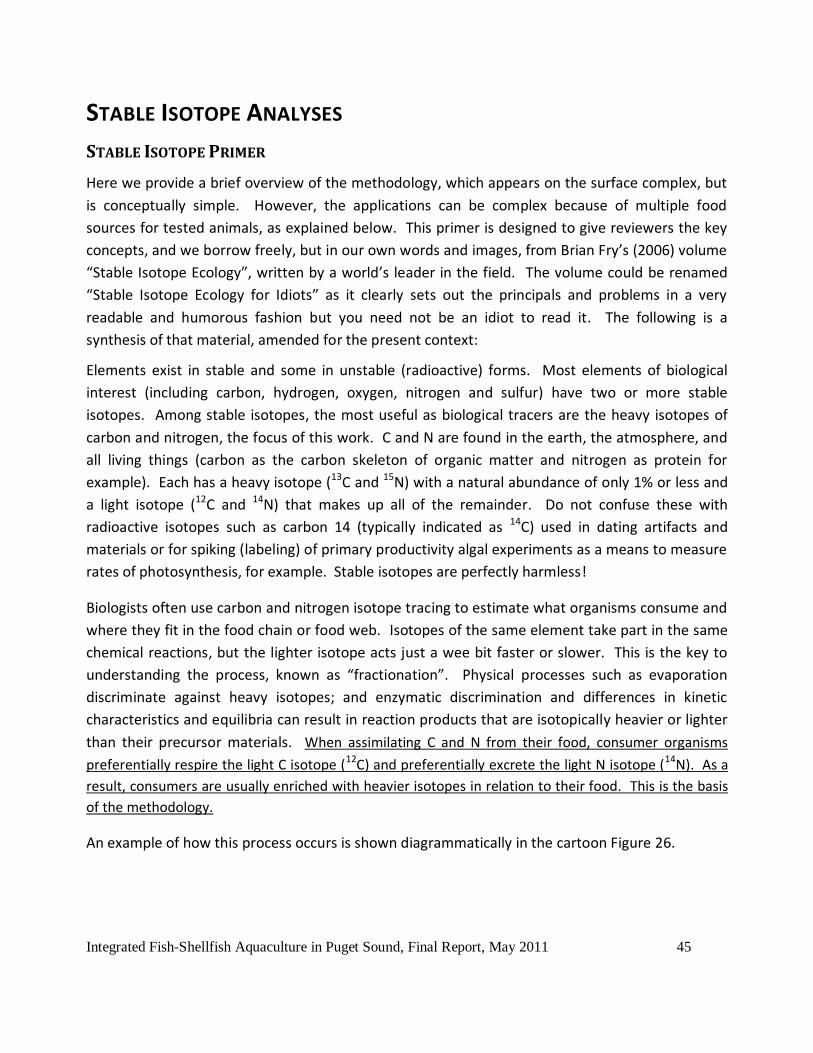
Integrated Fish-Shellfish Aquaculture in Puget Sound, Final Report, May 2011 45
STABLE ISOTOPE ANALYSES
STABLE ISOTOPE PRIMER
Here we provide a brief overview of the methodology, which appears on the surface complex, but
is conceptually simple. However, the applications can be complex because of multiple food
sources for tested animals, as explained below. This primer is designed to give reviewers the key
concepts, and we borrow freely, but in our own words and images, from Brian Fry’s (2006) volume
“Stable Isotope Ecology”, written by a world’s leader in the field. The volume could be renamed
“Stable Isotope Ecology for Idiots” as it clearly sets out the principals and problems in a very
readable and humorous fashion but you need not be an idiot to read it. The following is a
synthesis of that material, amended for the present context:
Elements exist in stable and some in unstable (radioactive) forms. Most elements of biological
interest (including carbon, hydrogen, oxygen, nitrogen and sulfur) have two or more stable
isotopes. Among stable isotopes, the most useful as biological tracers are the heavy isotopes of
carbon and nitrogen, the focus of this work. C and N are found in the earth, the atmosphere, and
all living things (carbon as the carbon skeleton of organic matter and nitrogen as protein for
example). Each has a heavy isotope (13C and 15N) with a natural abundance of only 1% or less and
a light isotope (12C and 14N) that makes up all of the remainder. Do not confuse these with
radioactive isotopes such as carbon 14 (typically indicated as 14C) used in dating artifacts and
materials or for spiking (labeling) of primary productivity algal experiments as a means to measure
rates of photosynthesis, for example. Stable isotopes are perfectly harmless!
Biologists often use carbon and nitrogen isotope tracing to estimate what organisms consume and
where they fit in the food chain or food web. Isotopes of the same element take part in the same
chemical reactions, but the lighter isotope acts just a wee bit faster or slower. This is the key to
understanding the process, known as “fractionation”. Physical processes such as evaporation
discriminate against heavy isotopes; and enzymatic discrimination and differences in kinetic
characteristics and equilibria can result in reaction products that are isotopically heavier or lighter
than their precursor materials. When assimilating C and N from their food, consumer organisms
preferentially respire the light C isotope (12C) and preferentially excrete the light N isotope (14N). As a
result, consumers are usually enriched with heavier isotopes in relation to their food. This is the basis
of the methodology.
An example of how this process occurs is shown diagrammatically in the cartoon Figure 26.

Integrated Fish-Shellfish Aquaculture in Puget Sound, Final Report, May 2011 46
Figure 26. Cartoon of heavy 13Carbon with one
more proton than light 12Carbon isotope, with red
circle representing neutron mass of each and the
teeter totter illustrating the relative weights
(after Fry 2006, but drawn from scratch).
So what does this mean in practical terms? It means that the difference between the light and
heavy isotope values can be used to measure and sometimes trace the flow of C and N from a
source to the environment, in the sediments, and in food webs to a plant producer or animal
consumer.
If there are multiple sources of nutrient or food, and we have enough information, we can create a
“mixing model” to estimate the contribution of elements C and N to an organism’s body from a
source as discussed below. But often this is very difficult or impossible without extensive research
or ends up being too complex to be of practical use. Often the best use of stable isotope
methodology is lowest in the food web. Higher up there are complications as higher trophic level
organisms feed on a variety of sources, from multiple trophic levels. Stable isotope studies are not
cookbook science, every situation is unique and must be studied on its own and sometimes the
results simply do not make sense for a variety of known or unknown reasons.
Isotope ratios are reported in “delta” (notation that is defined as the “per mil (parts per
thousand or 1/10 of a percent, the same units used in tax levies) deviation from the recognized
isotope standard, atmospheric N2 for 15N/14N and Peedee Belemnite (a limestone found in S.
Carolina) for 13C/12C ratios. Herein we use the common notation for these units of “‰”. These are
internationally accepted standards that all laboratories use. So if there is no enrichment of heavy
marine derived N (known as “ DN”) for example, the values are low (for nitrogen). Values for C
are often negative, only because it is measured relative to the standard, which can be confusing at
first. Nitrogen isotopes are often more reliable indicators or predictors of the trophic level that an
organism occupies in the food web because of the large 15N enrichment from one trophic level to
another (Owens 1987, Peterson and Fry 1987). But sometimes C isotope measurements are useful
too, as in fish farms where most of the particulate waste has C but very little N (that is dissolved
instead). We pay for both of them in the analysis and let the chips fall where they may! A helpful
guideline is:

Integrated Fish-Shellfish Aquaculture in Puget Sound, Final Report, May 2011 47
Do not get hung up on the absolute values of these measurements, as you might be when
observing basic water quality results. We are more concerned with the observed sample
differences among treatment locations, with differences between treatment and reference
sites, and with fluctuations across different time periods.
It is important to emphasize that 15N and 13C isotopes do not pass through the food web intact,
except at the beginning in plant primary production (photosynthesis). As atmospheric N is fixed in
primary production, there is no fractionation in that process, hence the 15N values begin low and
increase as nitrogen passes up through progressively higher trophic levels.
Each time the element is digested and egested by a higher consumer, it is fractionated again; and
by measuring the ratio of the either set of isotopes, i.e., “normal” or light isotopes of C and N,
biologists may be able to detect who ate what. In the present case, we start with measured ratios
of both carbon and nitrogen, heavy to light isotope ratios in several potential fish food sources,
including fish feed, fish feces, phytoplankton, seston, etc. Some of these data come from
measurements we took in the field; others are collected from the literature. For example, the
feed, which is heavily influenced from fish meal and fish oil and other products that sometimes
creates a distinctive ratio (or not, it depends on local conditions), can sometimes be distinguished
from other food sources. Most fish waste N is excreted as ammonium and a little urea and about
½ of consumed C respired as carbon dioxide, and roughly equal amounts are retained as fish tissue
or egested as feces. The C and N compounds and molecules released are then subject to uptake
by primary producers (in the case of dissolved C and N) or consumers, who are further up the food
web. The fractionation occurs again so if the tracing system is working properly we expect an
enrichment or positive change in 15N and 13C each time the element goes through a trophic level
of the food web, so:
The higher the value, the greater the amount of heavy isotope. The lower the value,
the lower the amount of heavy isotope, or as Fry (2006) says “higher heavier, lower
lighter.”
For carbon, the result values are reported as negative, and the less negative ones represent more
marine origin isotope, i.e., they are enriched. The negative delta-C values result from the way
delta notation is calculated ((Rsample/Rstandard -1)*1000, where R is the ratio of 13C to 12C). It
just means that almost all samples have less 13C than the PeeDee belemnite standard which is an
unfortunate condition as the results are usually negative, but the same idea applies as with N,
higher values indicate enrichment, so another quasi-rule:
Integrated Fish-Shellfish Aquaculture in Puget Sound, Final Report, May 2011 48
If there is a single food source flowing one step up a food web, except from macronutrient
to plant, one may anticipate a fractionation result difference of ~ +3.5 0/00 (range 3 to 4) for
nitrogen and +0.5 0/00 (range 0.1 to 1.0) for carbon stable isotopes (DeNiro and Epstein
1978, DeNiro and Epstein 1981, Peterson and Fry 1987). Results rarely match these stated
means or ranges, so +/- 10/00 in both cases is considered reasonable and some species, such
as marine mussels, have less whole-body nitrogen fractionation, in the range of 1.2 to 2.5 0/
00 (Hill et al. 2008).
For example, an increased 15N of 3.5 0/00 for nitrogen , e.g., from -18 to -14.5 15N would
constitute a single food web trophic level enrichment, as if a fish ate an insect larvae that was in
turn feeding on periphyton or biofouling algae. Atmospheric N is isotopically lighter than plant
tissues, and soil 15N values tend to be higher still, suggesting that microbes discriminate against
the light isotope during decomposition. Non-nitrogen-fixing plants, which derive their entire N
from the soil N pool, can thus be expected to be isotopically heavier than nitrogen-fixing plants,
which derive some of their N directly from the atmosphere including the blue-green algae
(cyanobacterial) group.
Biologists are able to determine if one or two sources of feed are involved in a food web study by
preparing “dual isotope plots” which are little more than a scatter diagram with on one axis
and C on the other axis. Vertical and horizontal differences in distance in these plots can
represent trophic level jumps, if the sources are initially different in profile. If not, sorry, the
system doesn’t work so well. If there are three or more sources, then complex mixing models are
required, as are measurements for all the food sources likely contributing to the target organism
that is the study focus. In this manner we could distinguish 5 sources if we had 4 actual sources
characterized by baseline measures, with only one unknown remaining. These models are not,
however, simple but there are published models and freely available spreadsheet models to
accomplish this task. See EPA website for details.1
IsoSource, one such model, is a Microsoft Visual Basic software package which calculates ranges of
stable isotope source proportional contributions to a mixture. We can use IsoSource to generate
mixing models from our data. The program generates every possible combination of source
proportions, compares these with the observed mixture isotopic signatures, and reports all
combinations that successfully sum to the mixture signatures. These results are then presented as
a histogram of the distribution of all possible combinations of source materials." These histograms
1 http://www.epa.gov/wed/pages/models/stableIsotopes/isosource/isosource.htm)

Integrated Fish-Shellfish Aquaculture in Puget Sound, Final Report, May 2011 49
can provide quantitative information that gives us an idea of the relative proportions of each food
source ingested by the study shellfish.
If you are confused by the above, this primer has not served its purpose, but a quick search on line
will yield a PDF copy of the Fry (2006) volume which really is very readable. Reading individual
scientific papers will usually only confuse you more, unless you read Fry’s (2006) volume or a
similar volume to grasp the basics. So now we present the stable isotope results of the project,
beginning with hypotheses.
HYPOTHESES AND APPROACH
This work was designed to look for spatial differences in stable isotope enrichment as a measure
of how different food sources, potentially including fish farm feed and wastes, are incorporated
into the shellfish in our experimental treatments. The primary null hypothesis is that there is no
enrichment effect of the fish farm on the shellfish. This is determined simply by comparing results
from our experimental treatments (grown close to the farm) to our reference group (grown far
away from the farm). If we see significant statistical trends by regression analysis or other
parametric analyses, we reject the null hypothesis.
Secondly, we examine the amount of variation between source of N and C from the pens
compared to content of other food sources such as phytoplankton and seston. This gives us the
possibility of preparing a “mixing model” using IsoSource that will guide us on quantifying the
relative amount of the food web components that originate from the fish farm.
STABLE ISOTOPE ANALYSES
Initially, we theorized that 13C would be the best tracer in shellfish tissue near the fish farm, since
fish feces are rich in carbon but relatively poor in nitrogen as most is excreted as dissolved
nitrogen. Shellfish therefore would consume relatively less salmon waste nitrogen, so we would
not expect as much 15N enrichment or in this case, depletion, from consuming them.
Turning to real data from this study, in Figure 27 we see that replicate samples of fish feces
collected from fish at Clam Bay had a 13C content of -20.8‰. Fish feed was even more negative
and seston, which includes phytoplankton, was found to have a 13C content of about -21.3‰ at Clam Bay and about -23.1‰ at Cypress Island, based on monthly samples in 2009. Puget Sound
phytoplankton have a 13C content of approximately -20.3‰ (Carpenter and Peterson 1989). A figure illustrating the varying ranges of stable isotope signatures in different food sources can be seen in Figure 27. Appendix 6 contains all averaged replicate stable isotope data.
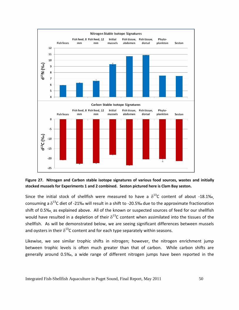
Integrated Fish-Shellfish Aquaculture in Puget Sound, Final Report, May 2011 50
Figure 27. Nitrogen and Carbon stable isotope signatures of various food sources, wastes and initially
stocked mussels for Experiments 1 and 2 combined. Seston pictured here is Clam Bay seston.
Since the initial stock of shellfish were measured to have a 13C content of about -18.1‰,
consuming a 13C diet of -21‰ will result in a shift to -20.5‰ due to the approximate fractionation
shift of 0.5‰, as explained above. All of the known or suspected sources of feed for our shellfish
would have resulted in a depletion of their 13C content when assimilated into the tissues of the
shellfish. As will be demonstrated below, we are seeing significant differences between mussels
and oysters in their 13C content and for each type separately within seasons.
Likewise, we see similar trophic shifts in nitrogen; however, the nitrogen enrichment jump
between trophic levels is often much greater than that of carbon. While carbon shifts are
generally around 0.5‰, a wide range of different nitrogen jumps have been reported in the

Integrated Fish-Shellfish Aquaculture in Puget Sound, Final Report, May 2011 51
literature. For our purposes, we assume a jump of 1.7‰ 15N, which is a value determined and
used in other stable isotope studies involving marine mollusks (Hill et al. 2008).
CLAM BAY
The set of four plots (Figure 28) below represent mean and SD of stable isotope 15N and 13C
values for Clam Bay oysters from September to the following January or June 2009. These figures
show consistent enrichment of 13C for all treatments compared to the initial measurement, and a
continual 13C enrichment as the experiment progressed. This only reflects the fact that 13C was
most likely lower for oysters’ diet at the hatchery location than at Clam Bay, and is not directly
relevant to our experiment. Similar to 13C, there was enrichment of 15N in the fall and early
winter of Experiment 1. But, by the experiment’s end in June 2009, 15N levels in all of the
treatments had dropped back down to initial levels or lower. Again, there is a possibility that this
is biologically significant, but likely not.
Figure 28. Clam Bay (CB) oyster carbon and nitrogen stable isotope results for January (mid experiment)
and June (experiment end) 2009 in Experiment 1, compared to initial values.

Integrated Fish-Shellfish Aquaculture in Puget Sound, Final Report, May 2011 52
Similar to oysters, fall period 15N enrichment of mussels was measured but by the end of the
experiment in June, 15N levels declined (Figure 29). In these mussels, 15N levels declined to
concentrations lower than initial values, suggesting an effect of feeding on the depleted 15N
sources discussed in the introduction to this section. The fact that both oysters and mussels are
responding similarly among seasons is evidence of a dietary shift that is at least in part, natural,
not net pen waste driven.
Figure 29. Clam Bay (CB) mussel C and N stable isotope Experiment 1 results, January and June 2009,
compared to initial values.
Clam Bay mussel results for Experiment 2 are presented in Figure 30. During the growing period
(April-September 2010, top left of Figure 30), nitrogen was depleted relative to initial values; it
subsequently went back to initial values when measured in March 2011 at the conclusion of the
experiment (top right of Figure 30). A much greater carbon enrichment was seen in the first half
of Experiment 2; the second half saw 13C falling back towards initial values.
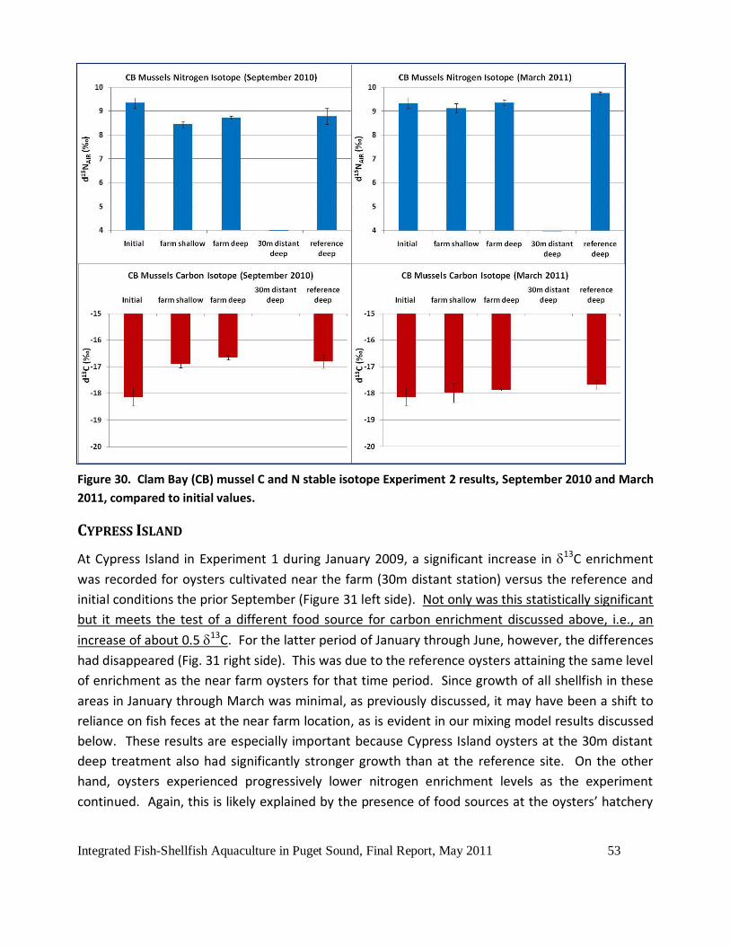
Integrated Fish-Shellfish Aquaculture in Puget Sound, Final Report, May 2011 53
Figure 30. Clam Bay (CB) mussel C and N stable isotope Experiment 2 results, September 2010 and March
2011, compared to initial values.
CYPRESS ISLAND
At Cypress Island in Experiment 1 during January 2009, a significant increase in 13C enrichment
was recorded for oysters cultivated near the farm (30m distant station) versus the reference and
initial conditions the prior September (Figure 31 left side). Not only was this statistically significant
but it meets the test of a different food source for carbon enrichment discussed above, i.e., an
increase of about 0.5 13C. For the latter period of January through June, however, the differences
had disappeared (Fig. 31 right side). This was due to the reference oysters attaining the same level
of enrichment as the near farm oysters for that time period. Since growth of all shellfish in these
areas in January through March was minimal, as previously discussed, it may have been a shift to
reliance on fish feces at the near farm location, as is evident in our mixing model results discussed
below. These results are especially important because Cypress Island oysters at the 30m distant
deep treatment also had significantly stronger growth than at the reference site. On the other
hand, oysters experienced progressively lower nitrogen enrichment levels as the experiment
continued. Again, this is likely explained by the presence of food sources at the oysters’ hatchery

Integrated Fish-Shellfish Aquaculture in Puget Sound, Final Report, May 2011 54
sites that were much more enriched in nitrogen than food sources available at Cypress Island.
Further investigation of Cypress Island oysters with IsoSource is discussed later in this report.
Figure 31. Cypress Island oyster stable isotope results for January (mid experiment) and June
(experiment end) 2009 in Experiment 1.
Unlike oysters, mussels in Experiment 1 experienced no differences between treatment and
reference 13C concentrations; therefore, no spatial effect of stable isotope enrichment from the
fish farm was likely, unless the effects were equally present throughout the sampled area (Figure
32). Similarly, in Experiment 2, there were no instances in which treatment groups were
significantly more enriched than the reference groups with respect to 13C and 15N (Figure 33).
Notably, Cypress Island mussels experienced the opposite from Clam Bay: all experimental 13C
concentrations were less enriched than the initial measurements. This suggests the possibility of
Cypress Island mussels sequestering significant amounts of farm wastes; which is supported by the
IsoSource analysis presented later in this report.
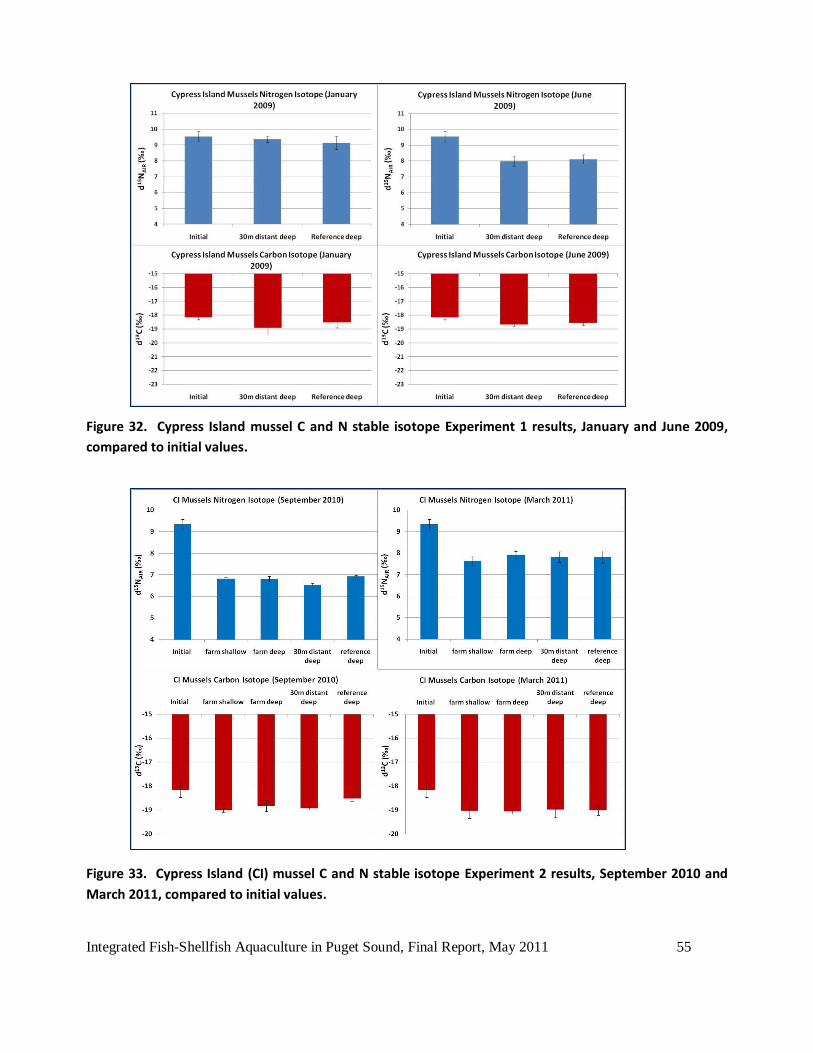
Integrated Fish-Shellfish Aquaculture in Puget Sound, Final Report, May 2011 55
Figure 32. Cypress Island mussel C and N stable isotope Experiment 1 results, January and June 2009,
compared to initial values.
Figure 33. Cypress Island (CI) mussel C and N stable isotope Experiment 2 results, September 2010 and
March 2011, compared to initial values.

Integrated Fish-Shellfish Aquaculture in Puget Sound, Final Report, May 2011 56
Overall, seasonal differences had much more of an effect on stable isotope enrichment by
separate 13C or 15N isotope than did treatment differences. With hindsight, even our reference
groups were probably much too close to the net pens. It is very possible that due to the very high
area currents, small dissolved particles and other material coming from the fish farms may be
carried a long distance before settling. The reference treatment may have received the same or a
similar amount of material as other treatments closer to the farms. However, our hypothesis may
remain valid. Diffusion and horizontal mixing studies in Puget Sound and the Gulf of Maine
indicate that a net pen “plume” can be initially uite narrow, so the 30m and reference locations
should have been in and out of the particulate supply of the net pens, depending on current
conditions.
In addition, seasonal differences are likely due to shifts in species composition of the
phytoplankton (e.g., spring phytoplankton blooms of diatoms versus summer and fall flagellates).
This was not an original focus of our study, and there is a surprising lack of literature that reports
isotopic values for different phytoplankton species.
Even if we do not factor in seasonal changes, we often saw enriched 13C and depleted 15N
compared to initial values (with the exception of Cypress Island mussels, which depleted 13C and
depleted 15N). It is most likely that 13C was lower in the shellfish’s diets at the original hatchery
locations, and that 15N was higher.
MIXING MODEL ANALYSES
The Visual Basic software package IsoSource was used for further analysis in an attempt to
determine the percentages of different food sources that the study shellfish were ingesting during
our experiments. By inputting known or estimated stable isotope signatures for a variety of food
sources, IsoSource can generate all possible combinations of source proportions and compare
these to the isotopic values of our sampled shellfish tissue, and then generate histograms of the
probability distribution, as well as the mean percentages of each food source. Food source
isotopic values, as well as shellfish isotopic values used in our IsoSource analysis, are found in
Table 3. Trophic level jumps were taken into account by decreasing our shellfish carbon values by
0.5 and nitrogen by 1.7, following accepted isotopic trophic jumps (Fry 1988, Raikow and Hamilton
2001, Moore and Suthers 2005, Hill et al. 2008).
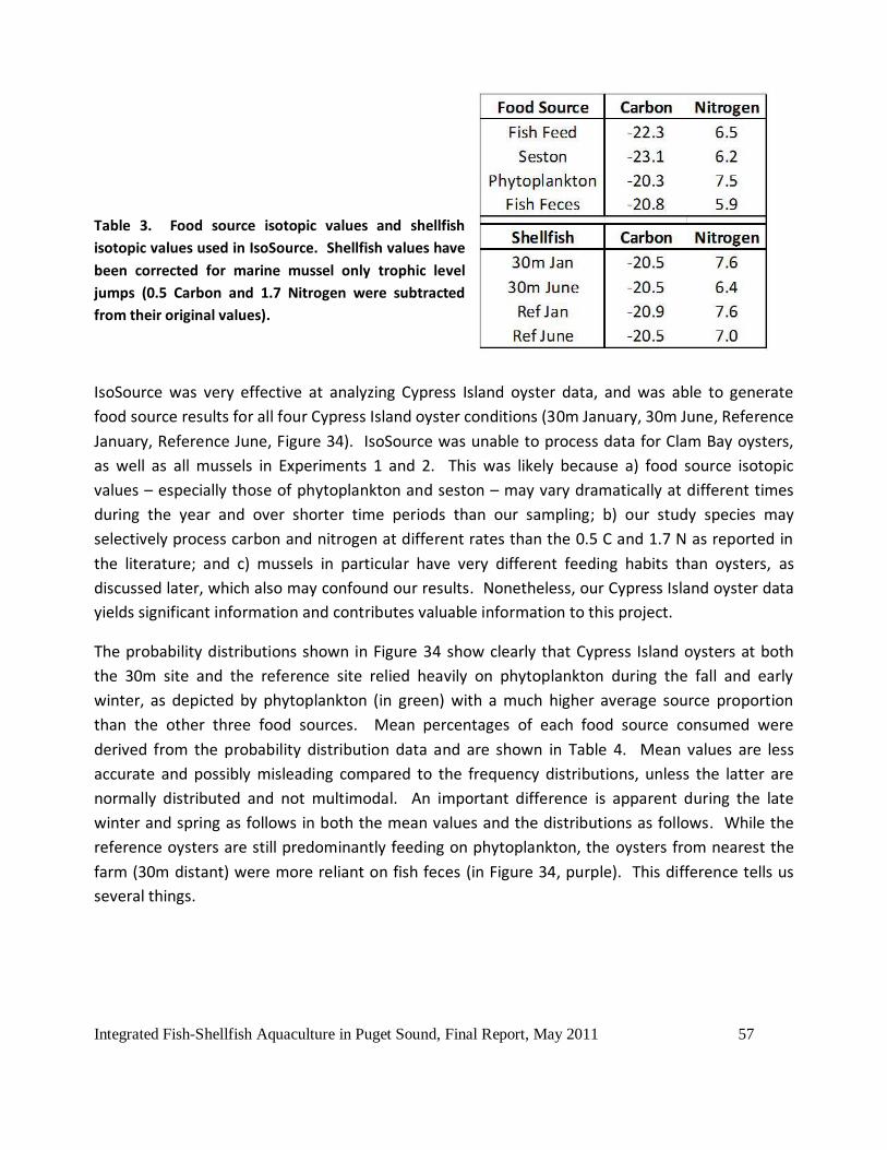
Integrated Fish-Shellfish Aquaculture in Puget Sound, Final Report, May 2011 57
Table 3. Food source isotopic values and shellfish
isotopic values used in IsoSource. Shellfish values have
been corrected for marine mussel only trophic level
jumps (0.5 Carbon and 1.7 Nitrogen were subtracted
from their original values).
IsoSource was very effective at analyzing Cypress Island oyster data, and was able to generate
food source results for all four Cypress Island oyster conditions (30m January, 30m June, Reference
January, Reference June, Figure 34). IsoSource was unable to process data for Clam Bay oysters,
as well as all mussels in Experiments 1 and 2. This was likely because a) food source isotopic
values – especially those of phytoplankton and seston – may vary dramatically at different times
during the year and over shorter time periods than our sampling; b) our study species may
selectively process carbon and nitrogen at different rates than the 0.5 C and 1.7 N as reported in
the literature; and c) mussels in particular have very different feeding habits than oysters, as
discussed later, which also may confound our results. Nonetheless, our Cypress Island oyster data
yields significant information and contributes valuable information to this project.
The probability distributions shown in Figure 34 show clearly that Cypress Island oysters at both
the 30m site and the reference site relied heavily on phytoplankton during the fall and early
winter, as depicted by phytoplankton (in green) with a much higher average source proportion
than the other three food sources. Mean percentages of each food source consumed were
derived from the probability distribution data and are shown in Table 4. Mean values are less
accurate and possibly misleading compared to the frequency distributions, unless the latter are
normally distributed and not multimodal. An important difference is apparent during the late
winter and spring as follows in both the mean values and the distributions as follows. While the
reference oysters are still predominantly feeding on phytoplankton, the oysters from nearest the
farm (30m distant) were more reliant on fish feces (in Figure 34, purple). This difference tells us
several things.

Integrated Fish-Shellfish Aquaculture in Puget Sound, Final Report, May 2011 58
Figure 34. IsoSource mixing model probability distribution histograms for Cypress Island oysters.
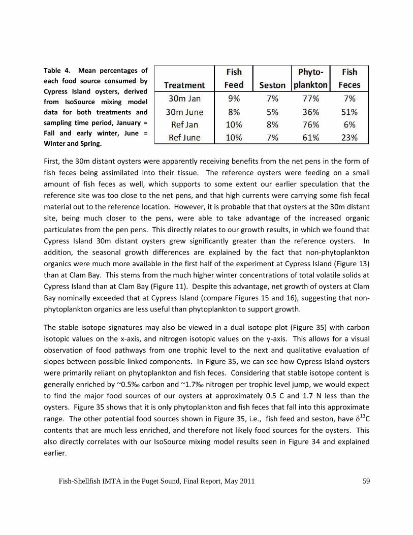
Fish-Shellfish IMTA in the Puget Sound, Final Report, May 2011 59
Table 4. Mean percentages of
each food source consumed by
Cypress Island oysters, derived
from IsoSource mixing model
data for both treatments and
sampling time period, January =
Fall and early winter, June =
Winter and Spring.
First, the 30m distant oysters were apparently receiving benefits from the net pens in the form of
fish feces being assimilated into their tissue. The reference oysters were feeding on a small
amount of fish feces as well, which supports to some extent our earlier speculation that the
reference site was too close to the net pens, and that high currents were carrying some fish fecal
material out to the reference location. However, it is probable that that oysters at the 30m distant
site, being much closer to the pens, were able to take advantage of the increased organic
particulates from the pen pens. This directly relates to our growth results, in which we found that
Cypress Island 30m distant oysters grew significantly greater than the reference oysters. In
addition, the seasonal growth differences are explained by the fact that non-phytoplankton
organics were much more available in the first half of the experiment at Cypress Island (Figure 13)
than at Clam Bay. This stems from the much higher winter concentrations of total volatile solids at
Cypress Island than at Clam Bay (Figure 11). Despite this advantage, net growth of oysters at Clam
Bay nominally exceeded that at Cypress Island (compare Figures 15 and 16), suggesting that non-
phytoplankton organics are less useful than phytoplankton to support growth.
The stable isotope signatures may also be viewed in a dual isotope plot (Figure 35) with carbon
isotopic values on the x-axis, and nitrogen isotopic values on the y-axis. This allows for a visual
observation of food pathways from one trophic level to the next and qualitative evaluation of
slopes between possible linked components. In Figure 35, we can see how Cypress Island oysters
were primarily reliant on phytoplankton and fish feces. Considering that stable isotope content is
generally enriched by ~0.5‰ carbon and ~1.7‰ nitrogen per trophic level jump, we would expect
to find the major food sources of our oysters at approximately 0.5 C and 1.7 N less than the
oysters. Figure 35 shows that it is only phytoplankton and fish feces that fall into this approximate
range. The other potential food sources shown in Figure 35, i.e., fish feed and seston, have 13C
contents that are much less enriched, and therefore not likely food sources for the oysters. This
also directly correlates with our IsoSource mixing model results seen in Figure 34 and explained
earlier.
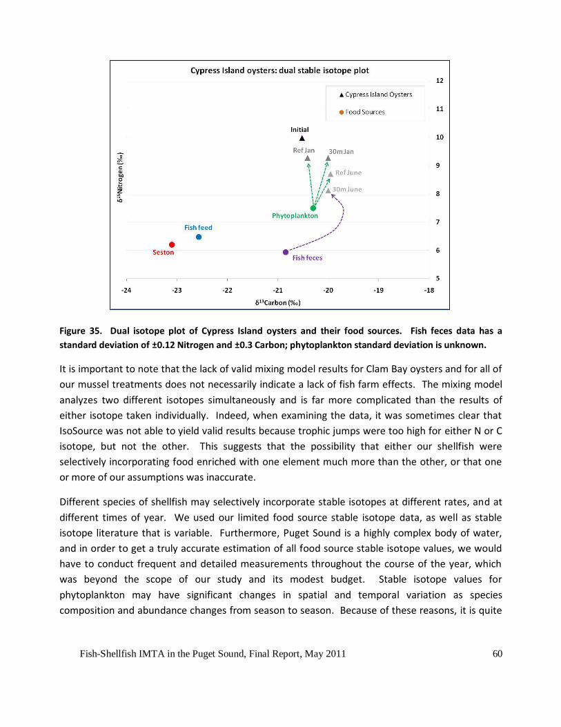
Fish-Shellfish IMTA in the Puget Sound, Final Report, May 2011 60
Figure 35. Dual isotope plot of Cypress Island oysters and their food sources. Fish feces data has a
standard deviation of ±0.12 Nitrogen and ±0.3 Carbon; phytoplankton standard deviation is unknown.
It is important to note that the lack of valid mixing model results for Clam Bay oysters and for all of
our mussel treatments does not necessarily indicate a lack of fish farm effects. The mixing model
analyzes two different isotopes simultaneously and is far more complicated than the results of
either isotope taken individually. Indeed, when examining the data, it was sometimes clear that
IsoSource was not able to yield valid results because trophic jumps were too high for either N or C
isotope, but not the other. This suggests that the possibility that either our shellfish were
selectively incorporating food enriched with one element much more than the other, or that one
or more of our assumptions was inaccurate.
Different species of shellfish may selectively incorporate stable isotopes at different rates, and at
different times of year. We used our limited food source stable isotope data, as well as stable
isotope literature that is variable. Furthermore, Puget Sound is a highly complex body of water,
and in order to get a truly accurate estimation of all food source stable isotope values, we would
have to conduct frequent and detailed measurements throughout the course of the year, which
was beyond the scope of our study and its modest budget. Stable isotope values for
phytoplankton may have significant changes in spatial and temporal variation as species
composition and abundance changes from season to season. Because of these reasons, it is quite

Fish-Shellfish IMTA in the Puget Sound, Final Report, May 2011 61
possible that proximity to fish net pens had some significant effect on our other shellfish groups,
even though IsoSource was unable to identify results.
DECISION MATRIX
After review the data extensively, we decided to focus our decision about efficacy of fish-shellfish
IMTA primarily on shellfish growth and stable isotope mixing model results. Other aspects of this
experiment, such as survival and stable isotope analyses, were judged not as important because
they showed few or no significant differences among treatments, but rather differences among
sites. Differences between sites are indeed important to try to tease out forcing factors, but
indicate that other factors – such as temperature, phytoplankton quality/quantity, etc. – were the
primary drivers of any observed differences. As this project was modestly funded, we had no
initial intention of attempting to measure all factors that would influence the above parameters.
An example would be sampling for phytoplankton stable isotope composition and species
composition on a weekly basis. This would be required to adequately describe average and
variable conditions that fluctuate greatly no doubt. Instead, we opted to use literature values for
phytoplankton but did collect extensive seston data.
Table 5 shows a matrix used to differentiate between significant and non-significant results of the
IMTA experiment. For clarity, and to distinguish our stable isotope analysis from our stable
isotope mixing model results, the single stable isotope analysis was not included in the matrix, i.e.,
we did not include separate analysis of 13C and 15N results. We conducted this analysis but found
that the results would sometimes conflict with the dual isotope mixing model analysis, which we
believe to be more powerful. However, a case could be made that proportionately much more
carbon was flowing from the pens in particulate form than nitrogen, as waste feces and feed is rich
in C but most N is excreted as dissolved form and therefore theoretically not as available to the
adjacent shellfish. This remains a research topic to be explored.
Shellfish survival, while also not very significant compared to our mixing models and growth
results, was included as a lower ranking factor in our final decision as to efficacy of the IMTA in
Puget Sound. In Table 5, cells marked with a + indicate the presence of significant differences
between experimental groups within a site and time period and those marked with a - indicate no
significant differences.
Table 5 clearly indicates that most significant IMTA results stem from oysters in Experiment 1.
Statistically significant growth was observed for oysters for both locations in the fall to early winter
period, and for winter to spring at Cypress Island. Even at Clam Bay in winter to spring growth was

Fish-Shellfish IMTA in the Puget Sound, Final Report, May 2011 62
nominally greater, but not quite statistically significant for the 30 meter distant and deep oysters
that did well in other time periods and at Cypress Island.
Table 5. Decision matrix that differentiates between significant and non-significant results.
Other notable results presented in Table 5 involve growth of Clam Bay oysters in the fall of
Experiment 1, and the survival of Clam Bay mussels in Experiment 1. However, unlike our Cypress
Island oyster results, multiple aspects of our experiment supported neither of these results.
Despite this, we can speculate about these outcomes as follows:
As explained previously in the growth results section above, Clam Bay oysters experienced a
significant stepwise growth trend during the beginning of Experiment 1, with progressively greater
growth the closer the oysters were to the fish farms. However, this difference between
treatments disappeared as Experiment 1 continued, and by the experiment’s end, there was no
significant difference between any of the Clam Bay oyster treatments. We may still tentatively
Fish-Shellfish IMTA in the Puget Sound, Final Report, May 2011 63
conclude that the significant growth present in the first part of the experiment is due to the fish
farm – but we cannot be sure, since other results did not correlate with the growth results in this
case except for nominally greater growth at the 30 m distant and deep station (again).
Likewise, Clam Bay mussels during Experiment 1 experienced some significant survival differences
among treatments. During the fall of Experiment 1, reference mussels had a lower average
mortality count compared to mussels closer to the farm, but in the following spring, the opposite
occurred and reference mussels had significantly higher mortality counts than the other treatment
groups. Because these results do not correlate with growth results or stable isotope analysis,
however, it is unlikely that this was related to the net pens, and is more likely due to some other
localized factor. In addition, when we transform the mortality count data into percentage of total
mortalities per day, the differences between treatments become much less pronounced.
Despite the lack of significance differences among treatments for mussels, the fact that oysters at
Cypress Island – and perhaps at Clam Bay as well – did experience greater growth at areas closer
to the fish pens is an indication that IMTA may confer significant benefits to oyster production and
particulate waste load reduction.
FURTHER INTERPRETATION
A unique aspect of Experiment 1 was the concurrent culture of mussels and oysters and the
finding that oysters successfully used fish farm wastes and grew better at one of the sites. Here
we compare our results to prior efforts to illustrate differences and parallels when possible.
OYSTERS
We tentatively conclude that oyster culture is technically feasible at representative net pen sites in
Puget Sound and that some proportion of the particulate waste produced by the fish farms is
captured and utilized by these shellfish. Oysters grew statistically faster and had stable isotope
profiles nearer the net pens that indicated direct use of fish feces at Cypress Island all year and for
part of the year at Clam Bay in terms of increased growth. Pacific oysters are readily available as
seed stock from local hatcheries and are hearty and well suited for raft culture near fish farms in
Washington State that are presently in protected, but very physically active sites exhibiting little or
no measurable adverse water column or benthic effects as discussed above.
We are not the first to examine oyster growth at Pacific Northwest fish farms. Jones and Iwawa
(1991) grew oysters at a fish farm in Jervis Inlet, British Columbia that is a fjord-like inlet on the
east side of the central Strait of Georgia. Their report is sometimes cited as evidence that IMTA is
Fish-Shellfish IMTA in the Puget Sound, Final Report, May 2011 64
a successful method. One publication stated, “Jones and Iwama (1991) found that oysters grew
three times the amount in shell height and growth rate when integrated with salmon farms than at
reference sites. This increase in weight and growth of the co-cultured species is a positive side
effect and holds obvious economic benefit for farmers” (Source intentionally not cited).
The subject inlet, like Sechelt Inlet of B.C. that was once the center of a thriving net pen industry in
the 1980s, is subject to seasonally intensive vertical stratification that can lead to micro flagellate
and dinoflagellate blooms. Since that time, all but one of the fish farming operations has moved
out of the area. Upon closer examination, the paper clearly shows that phytoplankton (measured
as chlorophyll a) concentrations were most strongly linked to growth of the different treatments
of oysters (increase in shell height) but curiously, monthly growth rate was correlated strongly to
particulate organic matter associated with each treatment of reference. These conflicting results
are not rationalized in the paper. We highlight these results because the site characteristics are so
different from Puget Sound sites, as discussed below.
MUSSELS
The use of gallo mussels to capture wastes at these same fish farms was apparently ineffective for
sequestering particulate wastes from the fish farms in the present study, both in terms of growth
(shell length) and for stable isotope effect. An assumption explicit in this and some prior studies
has been that accelerated growth of shellfish nearer to fish farms is demonstrative of IMTA
efficacy. Typically, the species of choice has been mussels of the genus Mytilus. Food quality and
quantity and water temperature are key factors controlling shellfish growth rate, but the former
(food quality) is difficult to assess.
We were unable to find more than a few published or unpublished cases of fish/mussel IMTA
resulting in accelerated growth near farms as others have reported (see review portion of Troell
and Norberg 1998). In some cases, positive results have been reported but no data or only limited
hydrographic information was provided on the study site, which is not helpful in terms of
understanding why the result occurred. There is a common thread explaining this variation and it
has to do with the background trophic status of the culture and/or reference areas in such studies.
Sara et al. (2009) reported accelerated growth of mussels near cages in the Mediterranean Sea on
the south coast of Sicily. This area is clearly oligotrophic with low concentrations of nutrients. It
has a deep mixed layer and nutricline and no large rivers nearby to supply major inputs of nitrogen
or phosphorus. Background chlorophyll a concentrations were near low at ~ 1 µg/L during their

Fish-Shellfish IMTA in the Puget Sound, Final Report, May 2011 65
study that occurred over one year. In contrast, average chlorophyll a concentrations at Clam Bay
and Cypress Island were approximately 2-3 times greater in the present study and dissolved
inorganic nitrogen was always >10 µM due to natural, oceanic sources as explained in this report.
Similarly, Peharda et al. (2007) measured growth and condition index of Gallo mussels grown near
fish cages in the eastern Adriatic Sea, an arm of the Mediterranean Sea of reduced salinity and
reportedly increased productivity (compared to the relatively barren Mediterranean Sea in most
regions) but they did not measure TVS, TSS or chlorophyll a. They found that mussels nearest the
pens grew slower than those 60m distant and not much different from reference mussels 600m
away. Condition index results were better nearest the pens during September through April but
other times exhibited mixed results.
Intuitively, one would expect shellfish grown in oligotrophic waters with low phytoplankton and
seston concentrations to be poor. In such areas, placing shellfish near fish farms that produce
particulate and in some cases dissolved inorganic or organic nutrients that could embellish
phytoplankton would be logical. But in moderate to fully eutrophic conditions, shellfish are not
necessarily reliant on fish farm wastes, particularly during the plankton growing season, so we
should not a priori expect that the shellfish will perform the service of fish farm waste removal in
such cases.
FEEDING SELECTIVITY AND OTHER EXPLANATIONS
Several factors may account for the lack of growth or stable isotope effect of cultured mussels in
our study besides background phytoplankton and seston quantities. Selective feeding behavior of
mussels may have been an issue where the oysters probably differ. Literature involving shellfish
feeding ecology and selectivity is abundant and inconclusive in many cases, illustrating few
constants among studies, locations and species. We note, however, that naturally occurring
oysters have evolved and are often cultured extensively to be epibenthic organisms. Mussels may
occur on any surface or submerged littoral zone but tend to occur (in Puget Sound) off bottom, on
rocks, floating objects, and other non-benthic locations where they often grow in great abundance
as a contiguous population. While this may be due to predation and survival, oysters normally
ingest suspended and resuspended living and decaying organic material whereas mussels, being
located higher in the water column on rocks or other natural structures, would be less likely to
evolve feeding strategies that focus on epibenthic detritus. There are many exceptions to this in
other regions.
It is likely that mussel are not selective “feeders” in terms of sorting particles upon ingestion but at
high seston or phytoplankton availability, selection can occur in the form of excess pseudofeces

Fish-Shellfish IMTA in the Puget Sound, Final Report, May 2011 66
production, either because the food source is not suitable or simply that there is too much food
available (see citations in Ren et al. 2000). Our study was not designed to evaluate this aspect of
the feeding ecology of shellfish or to provide an extensive review of the literature that would be a
major study unto itself.
Arifin and Bendell-Young (2000) present an alternative view stating that feeding behavior (from
other cited studies) in many marine bivalves suggests that they possess a highly selective feeding
strategy that allows for selection of organic over inorganic particles when high quality and quantity
seston is available. When low quality/quantity of seston is available, feed shifts to include both
organic and inorganic particles of lower quality for ingestion. In the case of fish farms and
shellfish, this would be likely during the non-algal growing season in temperate waters.
We find attractive the conclusion of Troell and Norberg (1998) “… that environmental factors and
design of cultivation technology are of importance in integrated cultivation systems. The
availability of organic food particles have been mentioned as being the single most important
factor determining growth rate of mussels (Seed and Suchanek, 1992), and maybe the existence of
both temporal and spatial variation in food availability in natural water bodies can explain the
degree of success”. The lack of effect for stable isotope tracing of either mussels or oysters at
Clam Bay is not surprising as no detectable differences occurred between upstream and
downstream TSS, TVS or chlorophyll a measurements. But neither was a difference observed for
the Cypress Island site, yet oysters apparently grew better near the farm there than at a reference
location. We believe that is due to the higher level of solids in the water during the winter than at
Clam Bay although we had no net pen site versus reference site water quality data to assess the
differences.
We also believe that it is necessary to sample and analyze plankton very frequently to adequately
describe their dynamics, but that was well beyond the scope of this preliminary study. The lack of
more frequent than monthly quantification of the seston food sources that would be necessary in
order for a more accurate mixing model calibration. If fish farmers decide to scale up oyster
culture at fish farm sites, we recommend that a bimonthly sampling of water quality/stable
isotope signatures and oyster growth be conducted. Only in this manner can the food source and
stable isotope probabilities be quantified. Determining this for phytoplankton versus other seston
remains a difficult issue potentially confounding the estimates but in our study seemed not to be a
problem with adequate separation on the dual isotope plots

Fish-Shellfish IMTA in the Puget Sound, Final Report, May 2011 67
OPTIMUM SITING VERSUS IMTA?
A main point of the above review of Jones and Iwawa (1991) is during summer all of their
treatment and reference locations were located in a typical Pacific Northwest embayment habitat
with vertically stratification, water and nutrient poor surface water and “bust or boom”
phytoplankton production patterns (Rensel Associates and PTI Environmental Sciences 1991).
After spring diatom blooms, such waters have low phytoplankton biomass until dinoflagellate
blooms prevail in calm days of summer. These highly mobile flagellates may not be measurable
near the surface in many cases, as they vertically migrate to depth at night to obtain their
nutrients and sometimes form thin layers at depth or remain near the nutricline for extended
periods. We would expect increased shellfish growth near a fish farm in Jervis Inlet describe above
compared to a reference location under these circumstances. By one informed estimate, about
50% of the fish farms in B.C. are located in such environments, but none are allowed (or preferred)
in such areas in Puget Sound as previously described above. Puget Sound fish farm sites rarely
have flagellate blooms, except in extreme river flow years when the weather is extremely mild
(e.g., Rensel et al. 2010) and at such times large parts of the entire Salish Sea are subject to the
same conditions, not just the poorly flushed backwater bays.
In Washington State, fish farms are purposely located in non-nutrient sensitive areas where their
dissolved nitrogen wastes will not directly contribute to or initiate algal blooms as previously
discussed as a requirement of aquatic lands leasing of the Washington Department of Natural
Resources. These non-nutrient sensitive areas are, however, not the locations that shellfish
growers often prefer, but they tend to be in the remote inlets and embayments where the
shellfish growth is enhanced by recurring phytoplankton blooms throughout the growing season.
In the present experiment, we contrasted our TVS and TSS results to those in Totten Inlet, a
renowned mussel, oyster and clam growing area of southern Puget Sound. The fish farms studied
were in Central and North Puget Sound and tend to have lower phytoplankton production and
much lower seston concentrations than Totten Inlet. That should be a positive factor for success
of shellfish/fish IMTA at the fish farm sites but the evidence from Clam Bay for oysters and for
both sites for mussel suggests otherwise, that either the rate of supply was not sufficient or that
selective feeding and pseudofecal production resulted in no measurable gain versus reference
specimens.
Many locations where IMTA has been advanced as a means to reduce fish farm wastes are likely
comparable to the Jervis Inlet example above, e.g., Chilean fjords and bays, New Brunswick bays,
Mediterranean Sea water, etc. While IMTA in these environments is an improvement over existing

Fish-Shellfish IMTA in the Puget Sound, Final Report, May 2011 68
fish monoculture at sites without adequate waste assimilatory ability, we argue that not all
aquaculture venues are similar. We view this as an ill-informed one-size-fits-all-approach of calling
for IMTA as a solution to a problem that, in the case of the advanced farm siting policies and
procedures in Washington State, does not exist. See the Ocean Conservancy website and report2
in this regard for an example of citing IMTA as a broad-brush solution to a perceived, universal
problem.
Clearly there are tradeoffs in siting fish farms, but should not fish farms be located in areas
suitable to assimilate their organic particulate or dissolved nutrient wastes without the need for
additional strategies that may or may not be effective? From our review of the literature,
extensive experience in siting of aquaculture facilities, impact assessment and environmental
modeling of the same, it does appear that efficacy of IMTA varies inversely sustainability of fish
farm siting, so this sets up a conundrum.
Should regulators continue, as they have for decades in Washington State, to promote fish farm
location in areas where food web assimilation and adequate dispersion of wastes occur?
or
Should nutrient sensitive, poorly flushed areas be re-targeted as they were 30 years ago in the
Pacific Northwest?
The answer is clear for Washington State: there is no turning back the clock to sites that have
proven unsustainable in terms of benthic deposition and risky to the fish farmer for fish survival,
even if IMTA methods were highly effective or predictable for waste removal, which presently by
any measure, they are not. Other factors such as naturally occurring harmful algal blooms that
often initiate in Pacific Northwest nutrient-sensitive backwater areas would deter fish farmers
from the return to these areas in most cases regardless of the other considerations.
An analogy to this choice is as follows: automobiles once relied on a poorly conceived and
executed emission control systems for cleanup of tailpipe emissions. The industry has evolved
away from that approach into more efficient engines that are cleaner because they produce less
harmful waste and more completely combust the fuel.
Accordingly, there is a danger in promoting IMTA as a cure all for the supposed ailments of
aquaculture everywhere and in every case. Regulators and fish farmers in Puget Sound have
worked for 40 years to establish policies that result in more optimum fish farm siting. This is not
2 http://www.oceanconservancy.org/our-work/aquaculture/assets/pdf/oc_rfts_v11_single.pdf

Fish-Shellfish IMTA in the Puget Sound, Final Report, May 2011 69
the case in many major fish farm producing countries where many sites are located in nutrient-
sensitive areas for whatever reason. Environmental NGOs often portray the fish farming industry
with one broad brush (e.g., the Monterey Bay Seafood Program, a perfect example), but there is
no monolithic, single industry to describe as such.
THE FUTURE FOR IMTA IN PUGET SOUND AND STRAIT OF JUAN DE FUCA
Despite the foregoing, IMTA could embellish fish farm environmental performance in Puget Sound
or similar environments (e.g., Cobscook Bay in Maine) even if the rate of fish farm waste removal
is less than optimum or as much as demonstrated herein for Cypress Island oysters. Even a low
rate of assimilation of wastes could, when scaled up appropriately, translate into an equivalent
increase in sustainable fish production. Although fish farmers will continue to rely on fish
production as their primary crop, having shellfish production nearby could also help diversify their
production as has been pointed out by IMTA advocates. IMTA could allow for additional expansion
within existing salmon aquaculture lease sites in some cases, but in other cases, new leases with
the State of Washington may have to be negotiated due to space limitation. The risk of expansion
would be on the fish farmer, as in any case benthic performance standards must be met or the
operation reduced in size, modified in configuration or relocated with new permits.
In open ocean aquaculture in some cases where current direction is highly variable, capture of fish
farm wastes is logistically more difficult and may have to involve complex pivoting systems to keep
the companion crops in line with the downstream currents. The open ocean is not a place for
complex, potentially cumbersome or poorly designed and built systems. In Washington State,
however, open ocean aquaculture means the oceanic conditions of the Strait of Juan de Fuca
(Rensel et al. 2007) where currents are strongly bidirectional and tidally driven for the most part.
In the very high current velocity Strait, oysters could potentially act as current deflectors up and
downstream of cages as tidal current passes through fish net pens and retain some particulate
waste production too.
In the relatively cool waters of Puget Sound main basins and channels where fish farms are
located, Pacific oysters rarely reproduce naturally thus would not add to the biofouling load on the
nets and floats that could occur with mussels when then reproduce. They could also be used in
some cases to provide current flow diversion at sites with overly strong currents or temporarily at
some sites where spring tides produce currents that exceed optimum velocities. Oysters will not
replace fish as a primary cash crop at fish farm sites due to space limitations, but subsurface
growing systems would benefit not only from the slowly settling organic particulate matter but
would be less subject to algal biofouling compared to surface raft culture of shellfish.

Fish-Shellfish IMTA in the Puget Sound, Final Report, May 2011 70
In other regions of the world, seaweed culture is also being practiced as a means to reduce
dissolved nitrogen loading. Puget Sound net pen sites are by design located in non-nutrient
sensitive areas but background levels of nitrogen are naturally high in main basins of Puget Sound.
The pen origin nitrogen plus the natural background flux of nitrogen could help insure a desirable
and continuous supply to insure sustained growth of seaweeds near the net pens. However,
combined shellfish plus seaweed culture at fish farm sites in Puget Sound may not be technically
feasible because of space limitations and the fact that seaweeds must be grown near the surface
to allow photosynthesis, whereas the shellfish are not subject to this limitation.
For Puget Sound waters, we recommend further investigation and scaled-up trials of the efficacy
of oyster culture as a companion crop to fish aquaculture. The trials to date with oysters have
been promising and we can envision several benefits from such systems as discussed herein.

Fish-Shellfish IMTA in the Puget Sound, Final Report, May 2011 71
REFERENCES CITED
Arifin, Z. and L.I. Bendell-Young. 2000. Influence of a selective feeding behaviour by the blue mussel Mytilus trossulus on the assimilation of 109Cd from environmentally relevant seston matrices. Marine Ecology Progress Series. 192: 181-193.
Brooks, K. 2008. Supplemental study of dissolved nutrients and particulate organic matter in the
waters near the proposed mussel farm in North Totten Inlet, Washington State, USA. Aquatic
Environmental Sciences, Port Townsend, WA.
Carpenter, R., and .L. Peterson. 1989. Chemical cycling in Washington’s Coastal Zone. pp. 367–
509 in Coastal Oceanography of Washington and Oregon, M. R. Landry and B.M. Hickey, eds.
Elsevier Science, New York.
Collias, E.E., N. McGary and C.C. Barnes. 1974. Atlas of physical and chemical properties of Puget
Sound and its approaches. Washington Sea Grant 74-1. Seattle.
DeNiro, M.J. and S. Epstein. 1978. Influence of diet on the distribution of carbon isotopes in
animals. Geochimica et Cosmochimica Acta 42: 495-506.
DeNiro, M.J. and S. Epstein. 1981. Influence of diet on the distribution of nitrogen isotopes in
animals. Geochimica et Cosmochimica Acta 45: 341-351.
Fry, B. 1988. Food web structure on Georges Bank from stable C, N and S isotopic compositions.
Limnology and Oceanography 33: 1182-1190.
Fry, B. 2006. Stable isotope ecology. First edition. Springer Publishing. 308 p.
Grant, J. and C. Bacher. 1998. Comparative models of mussel bioenergetics and their variation at field culture sites. Journal of Experimental Marine Biology and Ecology 219: 21-44.
Hawkins, A.J.S., P. Duarte, J.G. Fang, P.L. Pascoe, J.H. Zhang, X.L. Zhang and M.Y. Zhu. 2002. A
functional model of responsive suspension-feeding and growth in bivalve shellfish, configured
and validated for the scallop Chlamys farreri during culture in China. Journal of Experimental
Marine Biology and Ecology 281: 13-40.
Herlinveaux, R.H. and J.P. Tully. 1961. Some oceanographic features of Juan de Fuca Strait. Journal
of the Fisheries Research Board of Canada 18: 1027-1071.
Hill, J.M., C.D. McQuaid and S. Kaehler. 2008. Temporal and spatial variability in stable isotope
ratios of SPM link to local hydrography and longer term SPM averages suggest heavy
dependence of mussels on nearshore production. Marine Biology 154: 899-909.
Jones, T.O. and G.K. Iwama. 1991. Polyculture of the Pacific oyster, Crassostrea gigas (Thunberg),
with Chinook salmon, Oncorhynchus tshawytscha. Aquaculture 92: 313-322.

Fish-Shellfish IMTA in the Puget Sound, Final Report, May 2011 72
King, G. 2011. Taylor Shellfish, Personal communication to Z. Siegrist, March 2011.
MacDonald, B.A., S.M.C. Robinson and K.A. Barrington. 2011. Feeding activity of mussels (Mytilus
edulis) held in the field at an integrated multi-trophic aquaculture (IMTA) site (Salmo salar) and
exposed to fish food in the laboratory. Aquaculture 314: 244-251.
Moore, S.K. and I.M. Suthers. 2005. Can the nitrogen and carbon stable isotopes of the pygmy
mussel, Xenostrobus securis, indicate catchment disturbance for estuaries in northern New
South Wales, Australia? Estuaries 28: 714-725.
Nash, C.E. and F.W. Waknitz. 2003. Interactions of Atlantic salmon in the Pacific Northwest: I.
Salmon enhancement and the net-pen farming industry. Fisheries Research 62: 237-254.
NewFields Northwest. 2008. An assessment of potential water column impacts of mussel raft
culture in Totten Inlet. Prepared for Taylor Resources, Inc. Shelton, Washington. 96 pp.
Owens, N.J.P. 1987. Natural variations in 15N in the marine environment. Advances in Marine
Biology 24: 389-451.
Parametrix, Battelle Northwest Laboratories and Rensel Associates. 1990. Programmatic Environmental
Impact Statement: Fish culture in floating net-pens. Prepared for the Washington Department of
Fisheries. 161 pp.
Peharda, M., I Zupan, L. Bavcevic, A. Frankie and T. Klanjscek. 2007. Growth and condition index of
mussel Mytilus galloprovincialis in experimental integrated aquaculture. Aquaculture Research
38: 1714-1720.
Peterson, B.J. and B. Fry. 1987. Stable isotopes in ecosystem studies. Annual Review of Ecology
and Systematics 18: 293-320.
Raikow, D.F. and S.K. Hamilton. 2001. Bivalve diets in a Midwestern U.S. stream: a stable isotope
enrichment study. Limnology and Oceanography 46: 514-522.
Ren, J.S., A.H. Ross and D.R. Schiel. 2000. Functional descriptions of feeding and energetics of the
Pacific oyster Crassostrea gigas in New Zealand. Marine Ecology Progress Series 208: 119-130.
Rensel Associates and PTI Environmental Services. 1991. Nutrients and Phytoplankton in Puget
Sound. Peer reviewed monograph prepared for U.S. Environmental Protection Agency, Region
10, Seattle. EPA Report 910/9-91-002. 130 pp.
Rensel, J.E. 1996. Final Report: 1995 annual environmental assessment of Scan Am Fish Farms net
pen sites at Deepwater Bay and Skagit Bay, Washington. Prepared for Scan Am Fish Farms and
submitted to the Washington Department of Natural Resources. 38 pp. plus appendices.

Fish-Shellfish IMTA in the Puget Sound, Final Report, May 2011 73
Rensel, J.E., N. Haigh and T.J. Tynan. 2010. Fraser River Sockeye Salmon Marine Survival Decline
and Harmful Blooms of Heterosigma akashiwo. Harmful Algae 10: 98-115.
Ricciardi, A. and E. Bourget. 1998. Weight-to-weight conversion factors for marine benthic
invertebrates. Marine Ecology Progress Series 163: 245-251.
Sara, G., A. Zenone and A. Tomasello. 2009. Growth of Mytilus galloprovincialis (mollusca, bivalvia)
close to fish farms: a case of integrated multi-trophic aquaculture within the Tyrrhenian Sea.
Hydrobiologia 636: 129-136.
Seed, R. and T.H. Suchanek. 1992. Population and community ecology of Mytilus edulis. In:
Gosling, E. (Ed.), The Mussel Mytilus: Ecology, Physiology, Genetics and Culture. Elsevier,
Amsterdam, The Netherlands. pp 87-169.
Sutherland, T.F., A.J. Martin and C.D. Levings. 2001. Characterization of suspended particulate
matter surrounding a salmonid net-pen in the Broughton Archipelago, British Columbia. ICES
Journal of Marine Science 58: 404-410.
Taylor, A.H., R.J. Geider and F.J.H. Gilbert. 1997. Seasonal and latitudinal dependencies of
phytoplankton carbon to-chlorophyll a ratios: results of a modelling study. Marine Ecology
Progress Series 152: 51-66.
Troell, M. and J. Norberg. 1998. Modelling output and retention of suspended solids in an
integrated salmon-mussel culture. Ecological Modelling 110: 65-77.
WDF 1990. Fish Culture in Floating Net Pens. Washington Department of Fisheries. Final
Programmatic Environmental Impact Statement. Prepared by Parametrix, Battelle Pacific NW
Laboratories and Rensel Associates. For the Washington Dept. of Fisheries, Washington
Department of Natural Resources and Washington Department of Ecology. 161 pp.
Weston, D.P. and R.J. Gowen. 1988. Assessment and prediction of the effects of salmon net pen
culture on the benthic environment. Prepared for Washington Dept. of Fisheries. Appendix to
Final Programmatic Environmental Impact Statement. 62 pp. See also Modeling of Particulate
Deposition under salmon net pens by William P. Fox, P.E. in the same volume that provides
current vector information for the same site.
Welschmeyer, N.A. and C.J. Lorenzen. 1984. Carbon-14 labeling of phytoplankton carbon and chlorophyll a carbon: determination of specific growth rates. Limnology and Oceanography 29: 135-145.

Fish-Shellfish IMTA in the Puget Sound, Final Report, May 2011 74
APPENDICES
Appendix 1. Vertical profile data from Experiment 1. Data collected with a Hydrolab 4a with SCUFA in vivo chlorophyll a sensor.
December 2008 (lab samples taken for chlorophyll a at Clam Bay (coded as CB). S1 = the study site at Cypress Island (Site 1)

Fish-Shellfish IMTA in the Puget Sound, Final Report, May 2011 75
January 2009

Fish-Shellfish IMTA in the Puget Sound, Final Report, May 2011 76
March 2009 Clam Bay

Fish-Shellfish IMTA in the Puget Sound, Final Report, May 2011 77
Appendix 2. Water quality data for Clam Bay and Cypress Island.

Fish-Shellfish IMTA in the Puget Sound, Final Report, May 2011 78
Appendix 3. Mean and standard deviation of replicate shellfish lengths during measurement intervals.

Fish-Shellfish IMTA in the Puget Sound, Final Report, May 2011 79
Appendix 4. Mean and standard deviation of replicate shellfish mortality counts per each measurement interval.

Fish-Shellfish IMTA in the Puget Sound, Final Report, May 2011 80
Appendix 5. Mean and standard deviation of replicate mussel mortality lengths for measurement intervals of Experiment 2.

Fish-Shellfish IMTA in the Puget Sound, Final Report, May 2011 81
Appendix 6. Mean and standard deviations of replicate shellfish stable isotope results for each treatment within experiments.

Fish-Shellfish IMTA in the Puget Sound, Final Report, May 2011 82
Appendix 6, cont. Mean and standard deviations of replicate shellfish stable isotope results for each treatment within experiments.