©20

15N

atu

re A

mer

ica,

Inc.

All

rig

hts

res

erve

d.

protocol

102 | VOL.11 NO.1 | 2016 | nature protocols

IntroDuctIonShotgun proteomics has revolutionized biochemical and bio-medical research by enabling the identification and quantifi-cation of thousands of proteins in complex biological samples such as organelles, cell lysates, biological fluids and tissues1. The field’s denomination of shotgun proteomics describes a strategy developed in the Yates laboratory to characterize proteins that are analyzed indirectly through peptides obtained by pro-teolysis, in analogy to shotgun genomic sequencing2. The core of the discipline relies on state-of-the-art nanochromatography coupled with mass spectrometry, which is one of the most sensi-tive methods of analytical chemistry, in order to dissociate peptide ions in the mass spectrometer and to ultimately obtain peptide sequences; from these sequences, one can infer and quantify the proteins found in complex mixtures. Hundreds of thousands of tandem mass spectra are commonly generated in an experiment, and therefore advanced bioinformatics algorithms are required to make sense of all the data. In a typical experiment, peptides are fractionated by liquid chromatography on-line with tan-dem mass spectrometry, and protein identification is achieved by comparing experimental spectra against those theoretically generated from a sequence database. Proteins are then inferred by matching the identified peptide sequences to the sequences in the database; as peptides can match more than one protein, proteins can be further grouped according to a maximum parsi-mony criterion3. Peptide spectrum-matching (PSM) algorithms commonly leverage data from existing genomic projects. As a postgenomic discipline, the goals of shotgun proteomics are far more ambitious than those of genome sequencing, as shotgun proteomics aims to report protein expression, interaction, locali-zation, post-translational modifications, turnover time and so on, when comparing different biological states. During the past dec-ade, shotgun proteomics has been applied in many different ways to advance biological discovery. Notable examples can be found in studies describing differential protein expression between subcellular compartments4, pinpointing changes in proteomic

profiles of cancer biopsies5 and describing the contents of venoms to ultimately aid in biotechnological applications6,7.

The field was jump-started by the creation of SEQUEST, an algo-rithm that correlates tandem mass spectra with theoretical spectra generated from a sequence database8. In what followed, the coupling of strong cation-exchange chromatography with reversed-phase chro-matography on-line with tandem mass spectrometry set new heights in terms of the number of peptide identifications. This technology, later renamed as multidimensional protein identification technol-ogy (MudPIT)9, as well as competing strategies that use ultra-long chromatography gradients10, was adopted and thus raised the bar in terms of challenges, both in the handling of the new computational burden and in how to statistically deal with what was considered ‘big data’ at the time. In response, a new class of algorithms appeared, geared toward postprocessing the search engine results in order to statistically pinpoint identifications with confidence; examples of pioneering efforts are Peptide Prophet11 and DTASelect12. At the same time, breakthroughs on how to quantify complex peptide mixtures analyzed by mass spectrometry were being attained; the two main pillars of these breakthroughs were labeled and label-free approaches. Examples of the former are the isobaric tags13 and stable isotope amino acid labeling14, and examples of the latter are spectral counting15,16 and extracted-ion chromatograms (XICs)17. Naturally, intensive software development tailored toward enabling these quantification approaches became necessary. As the possibili-ties for how to mine the ‘proteomosphere’18 continued to expand, a plethora of new software programs began to be sparsely distributed among members of the community, each addressing very specific niches. These have included, for example, algorithms for scoring phosphosites19, deconvoluting mass spectra20 and even for dealing with unsequenced organisms18.

PatternLab and other widely adopted proteomic pipelinesWith so many options to choose from for analyzing shotgun pro-teomic data, efforts were shifted toward the creation of unified

Integrated analysis of shotgun proteomic data with PatternLab for proteomics 4.0Paulo C Carvalho1,2,7, Diogo B Lima1,7, Felipe V Leprevost1,3, Marlon D M Santos1, Juliana S G Fischer1, Priscila F Aquino4, James J Moresco5, John R Yates III5 & Valmir C Barbosa6

1Computational Mass Spectrometry Group, Carlos Chagas Institute, Fiocruz Paraná, Curitiba, Brazil. 2Laboratory of Toxinology, Oswaldo Cruz Institute, Fiocruz, Rio de Janeiro, Brazil. 3Department of Pathology, University of Michigan, Ann Arbor, Michigan, USA. 4Leonidas e Maria Deane Institute, Fiocruz Amazonas, Manaus, Brazil. 5Laboratory for Biological Mass Spectrometry, The Scripps Research Institute, La Jolla, California, USA. 6Systems Engineering and Computer Science Program, Federal University of Rio de Janeiro, Rio de Janeiro, Brazil. 7These authors contributed equally to this work. Correspondence should be addressed to P.C.C. (paulo@pcarvalho.com).

Published online 10 December 2015; doi:10.1038/nprot.2015.133

patternlab for proteomics is an integrated computational environment that unifies several previously published modules for the analysis of shotgun proteomic data. the contained modules allow for formatting of sequence databases, peptide spectrum matching, statistical filtering and data organization, extracting quantitative information from label-free and chemically labeled data, and analyzing statistics for differential proteomics. patternlab also has modules to perform similarity-driven studies with de novo sequencing data, to evaluate time-course experiments and to highlight the biological significance of data with regard to the Gene ontology database. the patternlab for proteomics 4.0 package brings together all of these modules in a self-contained software environment, which allows for complete proteomic data analysis and the display of results in a variety of graphical formats. all updates to patternlab, including new features, have been previously tested on millions of mass spectra. patternlab is easy to install, and it is freely available from http://patternlabforproteomics.org.

©20

15N

atu

re A

mer

ica,

Inc.

All

rig

hts

res

erve

d.

protocol

nature protocols | VOL.11 NO.1 | 2016 | 103

pipelines: indeed, deciding which software to pick and making them interact with one another were challenging problems. Thus, the first pipelines emerged, including the trans-proteomic pipe-line (TPP)21,22, OpenMS23, MaxQuant24,25 and PatternLab for proteomics26, each having its own set of advantages and limi-tations. In what followed, SkyLine27 and Galaxy28 emerged to overcome some of the limitations of the aforementioned tools at the time. Although there is great overlap among these software pipelines, each has a special set of features that provides advan-tages when analyzing data originating from a certain setup.

TPP and Galaxy are tailored to (but not limited to) working on computing clusters, thus relieving users from the burden of processing large amounts of data (and therefore vastly mobilizing resources, such as storage) locally on their own computers. As these tools are generally remotely accessed through a web-based interface or command-line tools, no requirements are imposed on the local operating system or hardware configuration. Through the years, several leading groups have worked together on devel-oping modules for TPP, and thus ultimately questions regarding details of how each module works can be addressed directly by the corresponding specialists. In contrast, the team behind Galaxy focuses on making available a customizable workflow management system, and thus efforts have been channeled toward providing a sophisticated environment for users to integrate several data analysis tools and protocols (as opposed to developing the data analysis modules themselves). In fact, this strategy culminated in making Galaxy an environment capable of integrating genomic, transcriptomic, proteomic and metabolomic data29.

In contrast, MaxQuant, OpenMS, Skyline and PatternLab are all designed exclusively to be used locally on one’s computer, with some clear benefits over their web-based counterparts. For example, when an update is done on a web-based pipeline, there is the possibility of immediate (and sometimes undesired) impact on ongoing analyses. Desktop users, on the other hand, have control over when to update their software. Moreover, it must be noted that today’s high-end desktops, and even notebooks, have become so powerful that they are fully capable of analyzing the data from large-scale proteomic experiments efficiently.

MaxQuant, Skyline and PatternLab all require Microsoft’s Windows 7 (or later) operating system, as they are based on .NET, which is a software framework that runs primarily on Microsoft Windows. In contrast, OpenMS can be executed on any operating system, as it is based on the C++ programming language. Another advantage of OpenMS is that its modules are all available as stand-alone tools, which facilitates integration into third-party workflows or the design of custom, local bioinformatics pipelines. As for the other tools, MaxQuant has been known to excel in stable isotope labeling by amino acids in cell culture (SILAC) experiments and Skyline in its unmatched capabilities in experi-ments addressing selected reaction monitoring (SRM) and parallel reaction monitoring (PRM). More recently, Skyline became capable of analyzing data-independent acquisition (DIA) data, as described in a previous protocol30. PatternLab, in turn, provides one of the most complete and user-friendly experiences, owing to its very refined and interactive graphical user interface. As for its hallmarks, we believe that they lie in analyzing label-free data through the T-Fold31 module and in the isobaric (e.g., isobaric tags for relative and absolute quantifi-cation (iTRAQ) or tandem mass tags (TMT)) analyzer module.

Some of its unique features include providing an integrated cloud service32, modules for statistically filtering and perform-ing assembly of de novo sequencing data33, statistically scoring phosphopeptides34, dealing with time-course experiments35 and offering a module for integrated Gene Ontology analysis36. Modules yet to be integrated in future versions are capable of dei-sotoping and decharging mass spectra18, and of identifying cross-linked peptides to address protein-protein interaction and to aid in providing structural data37 (the latter is described in a recent protocol38). Therefore, even though all mentioned tools, web- and desktop-based alike, overlap substantially with one another, each has its own hallmarks and unique features and may, as such, be more suitable for one’s working style and needs.

PatternLab is freely available software, and it is flexible enough to be used in the analysis of most shotgun proteomic experiments. We advise using PatternLab on any experiment requiring label-free quantification, or on experiments in which the data have been chemically labeled with isobaric markers.

Development of the protocolSince its launch in 2008, PatternLab has undergone continual improvement and expansion. The very first version was limited to working with spectral counting, and it offered strategies for pinpointing differentially expressed proteins, but all modules from that time have since been replaced by more sophisticated versions. Such major updates led us to release the system’s first major protocol in 2010 (ref. 39). Thanks to the continual influx of suggestions from their various users, the modules continued to evolve and new modules appeared, such as the Search Engine Processor40 (SEPro) for filtering and organizing shotgun pro-teomics data, and a module for XICs. A revised version of that first protocol was then published in 2012 (ref. 41). The PatternLab version at the time, PatternLab for proteomics 2.0, consisted of a series of modular software. A major request from its community of users was for the installation process of so many modules (one at a time) to be simplified. In addition, there was a desire for greater integration among the (then-independent) modules so that they would not have to be dealt with separately. Moreover, installing the modules could sometimes require installing third-party software such as the Java Runtime Environment, as well as having to deal with configuration files. Simply put, PatternLab needed to be reengineered to be completely installable at a single click of the mouse, as well as to work as a unit. PatternLab for proteomics 3.0 achieved this in 2013, by uniting all modules under a single graphical user interface and thus fulfilling all user requests of that time.

Since 2013, PatternLab has acquired new modules and func-tionalities. Some examples are as follows: Búzios, which allows the clustering of similar proteomic profiles5; the XD Scoring system, for evaluating the confidence in phosphosites34; PepExplorer, a tool for analyzing shotgun proteomic data of unsequenced organ-isms33; tools for performing analysis of variance (ANOVA); the incorporation of the Comet search engine, wrapped in a graphical user interface42, for analyzing isobaric experiments (e.g., iTRAQ and TMT); and a cloud service that enables large-scale quantita-tive predictions and comparisons of protein domains32. Some existing modules were significantly upgraded, such as the one for XICs. PatternLab for proteomics 4.0 is the culmination of these various changes; some of these changes are major, to the point of

©20

15N

atu

re A

mer

ica,

Inc.

All

rig

hts

res

erve

d.

protocol

104 | VOL.11 NO.1 | 2016 | nature protocols

spanning the complete workflow, but they always aim to simplify the process of analyzing shotgun proteomic data in an increas-ingly integrated environment . This protocol introduces the freely available PatternLab for proteomics 4.0, and it shows how to oper-ate the latest modules and how to deal with the new, simplified workflow. For those modules that underwent no changes, read-ers are referred to the corresponding sections of the previously published protocols.

Experimental designPatternLab is adaptable to many experimental designs, and as such it is applicable to analyzing data from most proteomic exper-iments. The topic of sample preparation and data acquisition in the mass spectrometer is an extensive one, and it encompasses tasks that must be performed before analyzing the data; in this regard, we recommend following the steps in the protocol by Richards et al.43.

Sequence database preparation. Databases of protein sequences are required so that theoretical mass spectra generated from them can be compared with experimental spectra. For the widely adopted PSM approach, we recommend downloading sequences from UniProt44, as some downstream analysis tools (e.g., the Gene Ontology explorer) can take advantage of this knowledgebase. Regardless, any type of sequence database in the FASTA format is supported, so users can download sequences from the US National Center for Biotechnology Information (NCBI) or even use an in-house-generated database. The UniProt knowledgebase comprises the Swiss-Prot and the TrEMBL databases; the former contains manually annotated and reviewed sequences, whereas the latter’s sequences are automatically annotated but not reviewed. We recommend downloading, whenever possible, only the species-specific database, which contains entries from both Swiss-Prot and TrEMBL. This is achieved by navigating to the UniProt website at http://www.uniprot.org, clicking on the large ‘Proteomes’ square, and then naming the species in the search box. The sequences can be obtained by clicking on the number in the ‘Protein count’ column beside the desired species, clicking on the download button, and then selecting the FASTA format. If wishes to use the Gene Ontology as a downstream tool, an additional download of the sequences, in the ‘Text’ format, must be done.

Subsequently, a target-decoy database must be generated before searching with PatternLab’s integrated version of Comet. PatternLab contains a module that allows the automatic genera-tion of decoys by reversing each sequence of the target database. A PatternLab option that we strongly recommend is to automati-cally include the 127 common contaminants found in proteomic experiments (keratin, BSA and so on). Even though there are many possible ways to generate decoy sequences, sequence reversal has been the most widely adopted one, as it conserves the complexity of the database (e.g., approximately the same number of decoy peptides and target peptides after an in silico digestion45).

Peptide identification from tandem mass spectra. PatternLab adopts Comet for the comparison of experimental and theo-retically generated mass spectra. Comet is a fast and sensitive open-source search engine that stemmed from the widely adopted SEQUEST8. Comet is constantly being updated, and PatternLab’s automatic updates may include an updated built-in Comet search

engine. A complete description of Comet’s parameters is available at the Comet project’s website http://comet-ms.sourceforge.net/parameters/parameters_201502/; PatternLab allows the setting of these parameters through its graphical user interface.

When searching for peptide candidates within a database, a precursor mass tolerance must be specified. When using high-resolution instruments such as an Orbitrap Velos (Thermo, San Jose), we recommend using no less than 40, even if the mass spectrometer used provides, say, 5 p.p.m. The suggestion for the adoption of wide search windows is empirical and comes from experimenting with the search engine. Nevertheless, our experi-ence is aligned with that of John S. Cottrell and David M. Creasy, from whom we quote, “The common observation is that FDR (false discovery rate) increases rather than decreases for very nar-row precursor tolerances because the reliability of the scoring is reduced by the small numbers of candidates”46. Finally, we note that Comet’s results will later be statistically filtered and postproc-essed by SEPro. At that final stage, any matching containing more than a tighter tolerance (e.g., 5 p.p.m.), will be discarded.

Peptides absent from the database cannot be identified by clas-sical PSM. The PSM strategy is therefore blind to mutations and polymorphisms, and it may not work satisfactorily on organisms that lack a reference peptide sequence database. Moreover, post-translational modifications must be specified a priori. Often these are unknown for the experiment at hand, so usually only carbami-domethylation of cysteine and oxidation of methionine are speci-fied as fixed and variable modifications, respectively. By having a quick look at UniMod (http://www.unimod.org), the protein modification for mass spectrometry database, one can take note of the variety of modifications that can occur in a sample. To cope with these limitations, approaches stemming from de novo sequencing have emerged. Among them we highlight Spectral Networks47, Mod-A48, MS-Blast49 and PepExplorer33. The first two are capable of pinpointing unanticipated modifications, whereas the last two start with de novo sequencing results and align them against sequence databases of homolog organisms so that similar proteins can be determined. In particular, PepExplorer is inte-grated into PatternLab’s workflow, but notwithstanding this we recommend that the user consider other applications when work-ing with unsequenced organisms. Being based on different para-digms, such applications may provide complementary results.

Statistically filtering peptide spectrum matches. The sensitivity of a PSM search engine is intimately related to how the search results are postprocessed. PatternLab relies on SEPro40 to statis-tically filter its results in order to achieve a predetermined FDR. The filtered results can be saved as a ‘sepr’ file and shared with collaborators. In this regard, anyone can open these files and have access to a dynamic report that enables sorting proteins accord-ing to various criteria (coverage, normalized spectral abundance factors, spectral counts, and so on), as well as access to annotated mass spectra and search engine scores, and also accomplish much more within a few clicks of the mouse. Even though PatternLab houses Comet, SEPro (and consequently PatternLab) is compati-ble with ProLuCID50, SEQUEST8 and the Spectrum Identification Machine for PITC51. Our 2012 protocol provides the main steps for using SEPro41. At the time of this writing, PatternLab still required several separate downloads for installation and relied mostly on ProLuCID, but SEPro has now been ported to the

©20

15N

atu

re A

mer

ica,

Inc.

All

rig

hts

res

erve

d.

protocol

nature protocols | VOL.11 NO.1 | 2016 | 105

main interface. Only the features that were implemented since 2012 are highlighted herein.

Quantitative proteomics. PatternLab can work with label-free quantification and with chemically labeled relative quantifica-tion. Among the label-free strategies, spectral counting has often been used in experiments with multidimensional separation (e.g., MudPIT). A spectral count refers simply to the number of tandem mass spectra associated with a protein, and it is used as a surrogate for the protein’s relative abundance. The community has proposed various ways for normalizing data of this type, and PatternLab optionally allows normalization by the normalized spectral abundance factor (NSAF) approach, which takes into account a protein’s length during the normalization process52. PatternLab also allows quantification by XICs, which are frequently used in single-shot experiments and are obtained by plotting the intensity of a given m/z value, plus or minus a given tolerance, over a given span of time. The area underneath this curve, or integral, can then be used as a surrogate for a peptide’s relative abundance in the mixture and as such provide a basis for comparison against the XIC of the same peptide in different mixtures.

A popular strategy for chemically labeling peptides to increase confidence in relative quantification has been the use of isobaric tags; PatternLab also makes available modules for analyzing such data. Examples of widely adopted, commercially available tags are iTRAQ13 and TMT53, which enable experiments to be mul-tiplexed. Currently, the most commonly adopted configurations are the 4-plex iTRAQ, 6-plex TMT and 8-plex iTRAQ; we point out that higher degrees of multiplexing are also available. These reagents rely on stable isotope-labeled molecules that covalently bind to the side-chain amines and the N terminus of polypeptide chains. PatternLab used to rely on the now deprecated SEProQ module (then available as a separate download) for dealing with XICs and isobaric tag data, but this module has been substantially re-designed and integrated into PatternLab for proteomics 4.0. A limitation of relative quantification by isobaric tags has been the interference of the nearly isobaric peptides that are cofrag-mented in the mass spectrometer along with the desired precursor ion, which generates a false relative quantification as the reporter ions’ signals get mixed with those from the nearly isobaric mol-ecules. To overcome this limitation, elaborate methods such as MultiNotch, which is only applicable to state-of-the-art or cus-tomized mass spectrometers, have been developed54. As far as we know, PatternLab’s isobaric module, described herein, is the only one to support MultiNotch acquisition while still providing a solution to standard data acquisition by automatically identifying and discarding multiplexed spectra.

The project must be organized in terms of what run belongs to which condition. This is performed using PatternLab’s Project Organization module, which ultimately generates a file that contains all identifications and the quantification data of all

runs from the entire experiment for use in downstream analyses by several modules. Examples of such analyses are clustering proteins or peptides with similar expression profiles for time-course experiments, clustering data, pinpointing differentially expressed proteins or proteins found in only one condition, performing ANOVA and even Gene Ontology analyses. In this protocol, we provide the main steps, highlighted in the graphical summary in Figure 1, involved in these analyses. An accompa-nying video, which demonstrates PatternLab for proteomics 4.0 in action, is available that provides an overview of the software (Supplementary Video 1).

Limitations of PatternLab for proteomics 4.0The following are the major limitations of the current PatternLab version:

• No handling of data from N15 labeling quantitative proteomic experiments.

• No handling of SILAC data.• No handling of SRM or PRM data55.• Not yet fully integrated with a public repository such as PRIDE56.

(i) Generate a target-decoysequence database (Steps 1–7)

.ms2

.mzML

.sqt

.sepr

.plp

.plp

(v) Spectral counting(Step 30A)

(v) Isobaric analyzer(Step 30C)

(v) XIC Browser (Step 30B)

(vi)

Búzios (Box 3)

Venn diagram (Box 3)

GO explorer (Box 5)

PatternLab for Proteomics

TrendQuest (Box 3) XD Scoring (Box 4)

PepExplorer (Step 30A)

ACFold/TFold (Box 3) ANOVA (Box 3)

(iv) Project organization (Step 30)

.sepr

(iii) Filtering Comet results withSEPro (Steps 21–29)

.T-R

.T-R

Database generation

Peptide identificationfrom

tandem m

assspectra

Statistically filtering P

SM

S/

Quantitating isobaric tags

Quantitation analyses:

Spectral counting/X

ICD

ata analyses

RAW files

(ii) Search with the integratedComet (Steps 8–20)

Thermo .raw

Figure 1 | Overview of PatternLab’s workflow. In a general workflow, a target-decoy database is prepared (i), the mass spectra are searched (ii) and statistically filtered to meet a user-defined FDR (iii), the project is organized in terms of which mass spectral files belong to what biological conditions (iv), quantitative information is extracted (v) and then the various downstream modules for data analysis can be used (vi). The main modules for database generation, peptide identification, statistical filtering and quantification of PSMs, and data analysis are presented. The protocol steps pertinent to each module are also given.

©20

15N

atu

re A

mer

ica,

Inc.

All

rig

hts

res

erve

d.

protocol

106 | VOL.11 NO.1 | 2016 | nature protocols

• Cannot handle top-down data (that is, mass spectrometry of intact proteins).

• The seamless integration with raw data from mass spectrom-eters other than those from Thermo requires exporting data to text-based formats such as MS2, mzXML, mzML or MGF.

• Requires a computer with Microsoft Windows 7 or later.

We are working to overcome most of these limitations, although we are not currently looking into addressing the third limita-tion, as Skyline already does a good job on that. Tackling the seventh limitation requires updates in the .NET environment from Microsoft’s end. The sixth limitation can be overcome by referring to the ProteoWizard project57.

MaterIalsEQUIPMENTHardware requirements

A personal computer with at least 6 GB of RAM and an ×86–64 processor crItIcal We strongly recommend having a multicore processor, as it can effectively deal with the parallel computation performed by some of the modules, and having at least 16 GB of RAM.Local storage is required for processing mass spectrometer RAW files. The space occupied by these files can vary substantially, depending on the mass spectrometer used

Data filesMass spectra data files in any of these formats: mzML58, mzXML, MS2 (ref. 59) or Thermo’s RAW

Software requirementsMicrosoft Windows 7 or later (64-bit version) crItIcal ‘Regional and Language Options’ have to be set to English, as several modules are tied to its decimal system..NET Framework 4.5 or later needs to be installed. The .NET Framework is made freely available by Microsoft; a new computer should already have this requirement fulfilled. Nonetheless, if the .NET Framework is

•

•

•

•

•

not detected during PatternLab’s installation, an attempt will be made to automatically install it through Microsoft’s website. The latest version, as of the time of this writing, is available from http://www.microsoft.com/en-us/download/details.aspx?id=42642Thermo Scientific MSFileReader should be installed in case the user wishes to work directly from the RAW instrument files. Instructions on obtaining this file are available from https://thermo.flexnetoperations.com/control/thmo/download?element=6306677

EQUIPMENT SETUPPatternLab setup Go to the PatternLab home page at http://patternlab forproteomics.org and click on the ‘Download’ link. If the .NET Framework 4.5 or later is already installed on the computer, clicking on the ‘launch’ link will automatically install PatternLab; otherwise, click on the ‘Install’ button. After PatternLab is installed for the first time, its main screen will pop up (Fig. 2). crItIcal Administrative access privileges are required for installation. crItIcal If PatternLab fails to install, you may need to update to .NET 4.5 or later. You can manually download and install the latest version of the .NET framework from Microsoft’s website.

•

proceDureGenerating a target-decoy sequence database ● tIMInG 5 s to several hours, depending on settings crItIcal A target-decoy sequence database must be generated before PSM.1| Click on ‘Generate Search DB’ in the upper-left corner of the interface. The sequence database module will load (supplementary Fig. 1).

2| Select an input database file format (UniProt, NCBI, and so on). A generic format called ‘Identifier Space Description’ can be used for any FASTA file.

3| Choose the output database format. We strongly recommend using the target-decoy approach that automatically includes a reverse version of each sequence in the database (with a ‘Reverse_’ attached to the beginning of the identifier). The other formats are made available for very specific purposes of software benchmarking.

4| Check the ‘Include common contaminants in the Targets’ checkbox to include the sequences of 127 common contaminants to mass spectrometry (e.g., keratins) at the beginning of the output sequence database.

Figure 2 | PatternLab’s main screen. The general PatternLab workflow is indicated by the order in which the pull-down menus appear. Generally, a target-decoy sequence database is prepared, searched with Comet and filtered to achieve a given FDR using SEPro or PepExplorer (in the case of de novo sequencing). The project is then organized in order to indicate which files belong to which biological condition. Downstream analysis is achieved by using the modules in the ‘Select and Analyze’ menus.

©20

15N

atu

re A

mer

ica,

Inc.

All

rig

hts

res

erve

d.

protocol

nature protocols | VOL.11 NO.1 | 2016 | 107

5| Click on the ‘Browse’ button in the Input group box and select sequence databases that were downloaded from the Internet. More than one database can be selected by pressing the Ctrl key while clicking on the file names in the file selection window.

6| Click on the ‘Save as’ button in the Output group box, and specify the name of the new database. A checkbox reading ‘Eliminate subset sequences’ is available for the elimination of sequences that meet a user-specified identity within other seq-uences in the database. When this happens, a note is appended to the remaining protein’s sequence description with a reference to the eliminated sequence. Specifying an identity below 100% will significantly increase the time for generating the database.

7| Press the ‘Go’ button to generate the new database. For proteogenomic studies, consider taking the extra measures described by Nesvizhskii60 so that the FDR is not underestimated. This is recommended.

performing psM with the integrated comet search engine ● tIMInG 1–2 min to >1 d, depending on sample complexity and equipment used8| Click on the ‘Search (Comet PSM)’ option from the main menu. The Comet graphical user interface will appear (Fig. 3).

9| Indicate a directory containing Thermo RAW, MS2, mzXML or mzML mass spectra files in the topmost textbox. The ‘Recursive Directory Search’ box must be checked for multiple directories to be searched.

10| Specify a target-decoy sequence database.

11| Specify a precursor mass tolerance. We suggest using the default 40 p.p.m., even for high-resolution mass spectrometers, as discussed in the INTRODUCTION.

12| For species-specific databases, set the parameter ‘Enzyme specificity’ to ‘semi-specific’. This is recommended, and it will increase the search space and reduce the search engine speed. However, having an estimate of how many semi-tryptic peptides were obtained after a tryptic digest can shed light on how well the sample was digested. If the sample was markedly degraded, we expect >20% of the peptides to be semi-specific. Contrasting with this, samples with no more than 5% semi-specific peptides should be taken as having undergone almost no degradation (optional; see Box 1). We note that some degradation is always expected.

13| Specify the number of missed cleavages allowed. We recommend allowing up to two misses for standard shotgun proteomic searches.

14| Specify the ‘Fragment Bin Tolerance’, ‘Fragment Bin Offset’ and ‘Theoretical Fragment Ions’ parameters. For low-resolution tandem MS, as generally provided in a Thermo LTQ, we recommend setting these values to 1.0005, 0.4 and ‘M peak only’, respectively. For high-resolution tandem MS, provided by a Thermo Q-Exactive, we recommend experiment-ing also with 0.02, 0 and ‘default peak shape’, respectively. The latter setting may slow the software substantially and, in our hands, it has usually led to little improvement in the search results.

15| Post-translational modifications (PTMs) should be specified by clicking on the ‘Add Modification from Lib’ button, which makes the modification library window pop up (supplementary Fig. 2). To select one or more PTMs, click on the corresponding row header, which highlights the entire row, and then on the ‘Add selected row to my Search.xml’ button. Figure 3 | PatternLab’s Comet search engine graphical user interface.

©20

15N

atu

re A

mer

ica,

Inc.

All

rig

hts

res

erve

d.

protocol

108 | VOL.11 NO.1 | 2016 | nature protocols

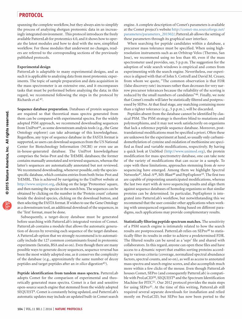
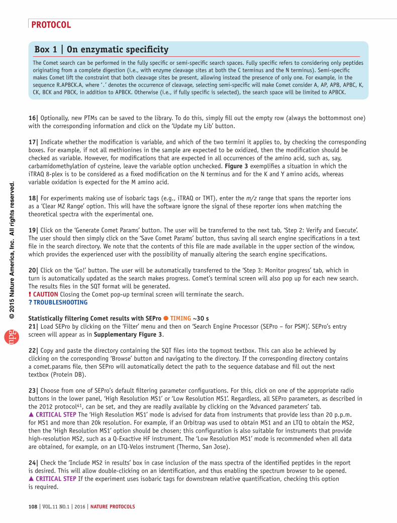
16| Optionally, new PTMs can be saved to the library. To do this, simply fill out the empty row (always the bottommost one) with the corresponding information and click on the ‘Update my Lib’ button.

17| Indicate whether the modification is variable, and which of the two termini it applies to, by checking the corresponding boxes. For example, if not all methionines in the sample are expected to be oxidized, then the modification should be checked as variable. However, for modifications that are expected in all occurrences of the amino acid, such as, say, carbamidomethylation of cysteine, leave the variable option unchecked. Figure 3 exemplifies a situation in which the iTRAQ 8-plex is to be considered as a fixed modification on the N terminus and for the K and Y amino acids, whereas variable oxidation is expected for the M amino acid.

18| For experiments making use of isobaric tags (e.g., iTRAQ or TMT), enter the m/z range that spans the reporter ions as a ‘Clear MZ Range’ option. This will have the software ignore the signal of these reporter ions when matching the theoretical spectra with the experimental one.

19| Click on the ‘Generate Comet Params’ button. The user will be transferred to the next tab, ‘Step 2: Verify and Execute’. The user should then simply click on the ‘Save Comet Params’ button, thus saving all search engine specifications in a text file in the search directory. We note that the contents of this file are made available in the upper section of the window, which provides the experienced user with the possibility of manually altering the search engine specifications.

20| Click on the ‘Go!’ button. The user will be automatically transferred to the ‘Step 3: Monitor progress’ tab, which in turn is automatically updated as the search makes progress. Comet’s terminal screen will also pop up for each new search. The results files in the SQT format will be generated.! cautIon Closing the Comet pop-up terminal screen will terminate the search.? trouBlesHootInG

statistically filtering comet results with sepro ● tIMInG ~30 s21| Load SEPro by clicking on the ‘Filter’ menu and then on ‘Search Engine Processor (SEPro – for PSM)’. SEPro’s entry screen will appear as in supplementary Figure 3.

22| Copy and paste the directory containing the SQT files into the topmost textbox. This can also be achieved by clicking on the corresponding ‘Browse’ button and navigating to the directory. If the corresponding directory contains a comet.params file, then SEPro will automatically detect the path to the sequence database and fill out the next textbox (Protein DB).

23| Choose from one of SEPro’s default filtering parameter configurations. For this, click on one of the appropriate radio buttons in the lower panel, ‘High Resolution MS1’ or ‘Low Resolution MS1’. Regardless, all SEPro parameters, as described in the 2012 protocol41, can be set, and they are readily available by clicking on the ‘Advanced parameters’ tab. crItIcal step The ‘High Resolution MS1’ mode is advised for data from instruments that provide less than 20 p.p.m. for MS1 and more than 20k resolution. For example, if an Orbitrap was used to obtain MS1 and an LTQ to obtain the MS2, then the ‘High Resolution MS1’ option should be chosen; this configuration is also suitable for instruments that provide high-resolution MS2, such as a Q-Exactive HF instrument. The ‘Low Resolution MS1’ mode is recommended when all data are obtained, for example, on an LTQ-Velos instrument (Thermo, San Jose).

24| Check the ‘Include MS2 in results’ box in case inclusion of the mass spectra of the identified peptides in the report is desired. This will allow double-clicking on an identification, and thus enabling the spectrum browser to be opened. crItIcal step If the experiment uses isobaric tags for downstream relative quantification, checking this option is required.

Box 1 | On enzymatic specificity The Comet search can be performed in the fully specific or semi-specific search spaces. Fully specific refers to considering only peptides originating from a complete digestion (i.e., with enzyme cleavage sites at both the C terminus and the N terminus). Semi-specific makes Comet lift the constraint that both cleavage sites be present, allowing instead the presence of only one. For example, in the sequence R.APBCK.A, where ‘ . ’ denotes the occurrence of cleavage, selecting semi-specific will make Comet consider A, AP, APB, APBC, K, CK, BCK and PBCK, in addition to APBCK. Otherwise (i.e., if fully specific is selected), the search space will be limited to APBCK.

©20

15N

atu

re A

mer

ica,

Inc.

All

rig

hts

res

erve

d.

protocol

nature protocols | VOL.11 NO.1 | 2016 | 109

25| Select the ‘Experiment with more than 50k spectra’ option in case it is estimated that there are ~50,000 or more mass spectra in the data; such volume is easily obtained when performing MudPIT experiments or using last-generation instruments (e.g., Orbitrap Elite) with long (3 h or more) gradients. This will make SEPro group identifications according to precursor charge state and enzymatic status (i.e., fully specific and semi-specific) in order to generate discriminatory functions that are independent of both charge state and enzymatic status.

26| Click on the ‘Go’ button. The user will be redirected to the ‘Follow up’ tab, where the tool’s progress is reported.? trouBlesHootInG

27| When the tool finishes processing, click on the ‘Result Browser’ tab to access the results (Fig. 4 and supplementary Fig. 3).

28| Save the results by accessing the ‘File’ menu and then by choosing ‘Save SEPro results’. Note that many formats are made available other than SEPro’s own; for example, one can save in the DTASelect format12 or in a tab-delimited file for use with spreadsheet software. crItIcal step If the user performed a ‘Batch Processing’ by checking the corresponding box in the entry page, the SEPro results files will be automatically saved to their corresponding directories. Batch processing is useful when there are several directories lying directly one level below a main directory; in this case, the user needs only to specify the path to filter the main directory, select the batch processing option and press the ‘Go’ button. Figure 4 shows SEPro’s graphical user interface while browsing through filtered results.

Figure 4 | SEPro’s Result Browser. SEPro provides a dynamic report that can be sorted according to any column. The top panel lists protein identifications, and clicking on any one of them causes the lower panel to display all matches associated with the corresponding protein, together with their respective scores. Double-clicking on a protein result brings up a window (in the upper-right corner) displaying a graphical coverage representation, a FASTA coverage representation and a group view (i.e., other proteins that share peptides). By double-clicking on a row in the lower panel, the annotated mass spectrum pops up. The lower-left corner displays one of the many new features in PatternLab for proteomics 4.0; clicking on the ‘Tools’ menu and then on ‘Evaluation of Enzyme Specificity’ will display a window informing how many fully specific, semi-specific and nonspecific peptides were identified in the mixture.

Box 2 | Project organization One of the goals of proteomics is the study of differences in protein expression throughout different biological states. Others include analyzing time series data or samples originating from different tissues. In this regard, PatternLab must be informed which samples come from which biological condition or point in time. The Project Organization module deals with this matter. For example, suppose that one performed a five-point time-course experiment with three biological replicates at each point. Data were acquired using 12-step MudPIT, and now the user wishes to perform relative quantification by spectral counting. This hypothetical experiment would encompass a total of 180 LC-MS/MA files. These files would need to be arranged in directories as follows. First, a directory for each time point would need to be created: for this example, say, T0, T1, T2, T3 and T4. Within each directory, directories for each biological replicate would also need to be created, so, for example, within the T0 directory we would create the directories T0B1, T0B2 and T0B3. (We urge the user not to provide simplified names as, say, B1, because this same name might ambiguously refer to B1 in directory T1 and some modules of PatternLab require each directory to have a unique name.) Finally, within T0B1, for example, the RAW files, SQT files and the sepr file would be placed. We note that this organization can also be arranged before using Comet; in this way, only the main directory would need to be provided and PatternLab would have Comet search within each directory (consequently making the SQT files already appear in the corresponding directories). Similarly, SEPro can perform batch filtering if the main directory is provided. Structuring the files as described enables PatternLab to ultimately compile a PatternLab project file, which contains cross-experiment identification and quantification data; in turn, these are required for downstream analysis. During the next steps of the protocol, the user should decide whether quantification should be performed by spectral counting, by XICs or through reporter ion signals provided by isobaric markers. Although the latter originates from sample preparation, the former two remain an open choice; we recommend using spectral counting for MudPIT experiments and XICs for single shots.

©20

15N

atu

re A

mer

ica,

Inc.

All

rig

hts

res

erve

d.

protocol

110 | VOL.11 NO.1 | 2016 | nature protocols

29| (Optional) A frequent community request has been for the user to be able to concatenate the results of several SEPro files. To do this, place the desired files in the same directory, select the option ‘SEPro Fusion’ from the ‘Tools’ menu and then click on the ‘Save new SEPro file’ button in the pop-up window. A new SEPro file will be generated that joins the data from all the SEPro files pertaining to that directory.

Quantification analysis using spectral counting, XIc or analysis of multiplex experiments with isobaric tags30| At this point, it is possible to choose option A for quantification analysis by spectral counting, option B for XIC or option C for analysis of experiments using isobaric labels. For project organization, see Box 2. Once this step is finalized, downstream data analysis involving differential proteomics (Box 3), scoring phosphopeptide sites (Box 4) or analyzing results under the light of the Gene Ontology (Box 5) is then possible.(a) Quantification analysis with spectral counting ● tIMInG ~20 s (i) Project organization. Click on the ‘Project Organization’ menu, and then on the ‘SEPro or PepExplorer’ button.

The interface will look like that shown in Figure 5. (ii) Include each directory, prepared as specified in Box 2, in the Input Control. For the example in Figure 5,

two biological conditions were inserted (i.e., BiologicalCondition1 and BiologicalCondition2). (iii) Include a brief (~10 words) description of the experiment in the Project Description text box. (iv) Click on the ‘Load’ button. (v) To obtain Spectral counting data for downstream analysis, click on the ‘Step 2: Spectral Counting’ tab. There you can

optionally select for NSAF52 normalization, and choose whether the quantification will be mapped at the peptide or protein level. Next, click on the ‘Go’ button, followed by the ‘Save PatternLab project’ button.

Box 3 | Differential proteomics using the ACFold/T-Fold/Venn diagram modules/principal component analysis ● tIMInG <3 s Once a PatternLab project file is generated, the ACFold or T-Fold31 and area-proportional Venn diagram modules can be used for pinpointing differentially expressed proteins and proteins exclusive to a biological condition, respectively. Other modules for performing ANOVA, principal component analysis (PCA) (Búzios) and for analyzing time-course experiment data (TrendQuest) are also available. These modules are all demonstrated in supplementary Video 1, and they have been described in our previous protocols, so we refer the reader to them41. Notwithstanding this, we note that these modules’ previous versions required the use of the ‘index.txt’ and ‘sparseMatrix.txt’ files to store all the identification and quantification data of the experiment. In the current version, they were replaced by a single PatternLab project file, generated in the Project Organization module as explained in Box 2. PatternLab for proteomics 4.0 provides a tool for migrating the legacy format to the updated PatternLab project file in the ‘Utils’ menu.? trouBlesHootInG

Box 4 | Scoring phosphopeptide localizations with the XD Scoring module ● tIMInG ~35 s Confidently determining phosphorylation sites is crucial to understanding the regulatory mechanisms in biological systems. PatternLab for proteomics 4.0 includes a false-localization rate probabilistic module, termed XD Scoring, that enables unbiased phosphoproteomics studies25. Briefly, the XD Scoring algorithm infers a probabilistic function from the distribution of the identified phosphopeptides’ XCorr delta scores (XD scores) and provides P values by relying on Gaussian mixture models and a logistic function. For a mass spectrum whose top-scoring candidate is a phosphopeptide, the XD score is calculated as the difference between the top two XCorr scores of alternative phosphorylation sites in the same peptide sequence. In this regard, for this module to work efficiently, we recommend having the search engine report at least the top 20 scoring candidates in its search results. When using the Comet search in PatternLab, this amounts to editing the line that starts with ‘num_output_lines = ‘ to indicate 20, after clicking on the ‘Generate Comet Params’ button.

1. Access the XD Scoring module by clicking on the ‘Utils’ menu and then on ‘XD Scoring (Phosphosite)’.2. Click on the ‘Load SQT files’ button and select the Comet results files by pressing and holding the ‘Ctrl’ key while left-clicking on the desired search results files.3. Click on the ‘Calculate’ button. A list containing the logarithms of the delta scores for all phosphopeptides will appear in the lower textbox.4. Click on the ‘Generate GMM’ button. This will enable PatternLab to generate a Gaussian mixture model whose two Gaussians come from a histogram on the natural logarithms of the XD score. At the bottom of the interface, a green curve shows the cumulative distribution of the green Gaussian and a red curve shows the complementary cumulative distribution of the red Gaussian (supplemen-tary Fig. 6). A complementary logistic function is then generated based on the former two distributions (purple curve). The desired P values are given by this function.5. Specify a SEPro file; this enables the program to output a table associating a P value to each site attribution.

©20

15N

atu

re A

mer

ica,

Inc.

All

rig

hts

res

erve

d.

protocol

nature protocols | VOL.11 NO.1 | 2016 | 111

(vi) Optionally, map spectral counts to protein domains by selecting the ‘Step 2: Differential Domain Expression’ tab. This tab offers controls that enable the generation of a PatternLab project file, as previously described32.

(B) Quantification analysis with XIc ● tIMInG ~30–40 s for each mass spectrum raw file (i) Follow Step 30A(i–iv). (ii) Click on the ‘Step 2: XIC Analysis’ tab if XICs are to be obtained. This tab offers controls that will ultimately produce

an XIC file, viewable within PatternLab’s XIC Browser module, which is available through the ‘Quant’ menu by selecting ‘XIC Browser’. The XIC Browser module is then used to generate a PatternLab project file, as described in the Using PatternLab’s XIC Browser section.

(iii) Click on the ‘Quant’ menu and then select ‘XIC Browser’. (iv) Click on ‘File’, and then on ‘Load’ and ‘Bin’ to load an .xic file generated using PatternLab’s Project Organizer.

This is a binary file by default, yet the XIC Browser allows files to be saved in the JavaScript Object Notation (JSON), which is a lightweight text-data-interchange format that simplifies the parsing by other software.

(v) Review the list of cross-experiment identified peptides that will appear as soon as the file finishes loading. Note that each column will be named after a search file (e.g., SQT) and list the XIC values for each peptide. Double-click on an XIC value to open an XIC plot together with a table discriminating the plotted values, as exemplified in Figure 6. The table discriminating the quantification values can also be copied and the values pasted onto some spreadsheet software.

(vi) Click on the ‘Graphical Analysis’ tab to view a histogram of the label-free quantification values for all peptides (supplementary Fig. 4). Note that many experiments can be simultaneously assessed.

(vii) Optionally, use the XIC Browser to reduce the effects from undersampling. Undersampling is a common problem in proteomics, as not all peptides are sampled by the mass spec-trometer. The XIC Browser can help with this limitation by relying on the retention times and precursor masses of peptides identified in a run to estimate the XIC of a peptide

Box 5 | The gene ontology explorer ● tIMInG ~5 min The Gene Ontology Explorer (GOEx) allows users to analyze their data under the light of the Gene Ontology; this module has been well documented21,40. In order to analyze the data, a ‘precomp’ object must be generated; this is done by joining the Gene Ontology OBO-format file (available at http://geneontology.org/page/download-ontology) with an annotation file. Our original version worked only with annotation files provided at the Gene Ontology website, but the updated GOEx module can work with any organism available in the UniProt base. As this has been the only update to this module, what follows pertains exclusively to the steps for generating a precomp file using UniProt.

1. Download the data for the desired organism from UniProt as previously described, but instead of selecting the FASTA format choose the text format.2. Download the latest Gene Ontology OBO file.3. Access the Gene Ontology by clicking on the ‘Analyze’ menu and then on ‘GOEx (Gene Ontology Explorer)‘. The GOEx interface will appear.4. Click on the ‘Load GO DAG’ button and select the GO.OBO file. This will cause GOEx to perform some optimizations that should take ~2 min.5. Click on the ‘Load Associations’ button; a window will pop up. The new option for using UniProt text files will be available and selected by default.6. Click on the ‘Browse for conversion file’ button and load the file downloaded from UniProt.7. Click on the ‘Save Precomp’ button. The next time a GO analysis is performed, instead of having to repeat all these steps the user can proceed directly to loading the precomp file by clicking on the ‘Load precomp’ button.8. Refer to the previous publications on GOEx36,39 for a complete set of instructions for operating this module.

Figure 5 | PatternLab’s Project Organizer. This module is responsible for joining the information of the various biological or technical replicates from all biological conditions. Directories containing results filtered by SEPro should be indicated for each biological condition.

©20

15N

atu

re A

mer

ica,

Inc.

All

rig

hts

res

erve

d.

protocol

112 | VOL.11 NO.1 | 2016 | nature protocols

in another run, one in which that peptide was not sampled. To accomplish this, first click on the ‘Completion’ tab; a list of all liquid chromatography–tandem mass spectrometry (LC-MS/MS) runs in the experiment will be provided in one column, along with another column to which the user can input a number for each run. Label the runs that should be grouped for inferring XICs by placing the same number beside each one (Fig. 7). Finally, click on ‘Filter’ and then on ‘Fill in the gaps’. The new XICs, completed by using the retention times and the precursor masses of peptides identified in compatible runs, will be listed in the XIC Browser in green. Identifications with no XICs, or XICs not passing a minimum quality criterion, will have values of -1 and be listed in red.

(viii) The same peptide is usually identified through different charge states and consequently with different precursor m/z values. The XIC Browser makes available an option, through the ‘Filter’ menu and then by selecting ‘Retain Optimum Signal’, for only the best (higher-value) XICs for a given charge state to be retained. So, for example, if in general the charge-(+2) peptide precursors for a given peptide have XIC values greater than their charge-(+3) counterparts, then all XICs from the latter version of that peptide will be discarded. Arguably, by considering only the more intense XIC versions of the peptide, less noise gets into the model and a more accurate relative quantification can be obtained (data not shown).

(ix) Click on the ‘File’ menu followed by ‘Save’ and then by ‘PatternLab project file’ to generate a PatternLab project file for downstream analysis.

(c) analyzing multiplex experiments labeled with isobaric tags ● tIMInG 20–50 s for each mass spectrum raw file crItIcal SEPro files to be analyzed with the ‘Isobaric module’ must have been processed using the ‘include MS2 in results’ option. (i) Click on the ‘Quant’ menu, and then on ‘Isobaric Analyzer’. (ii) If data were acquired according to the MultiNotch approach, extract the MS3 data from the RAW file. For this,

click on PatternLab’s ‘Utils’ menu, select the RawReader module, then check the ‘MS3’ checkbox and the directory containing the mass spectra raw files and click on the ‘Go’ button. We note that this step can also be accomplished by any software that is capable of extracting MS3 files, such as RawExtractor, for example, made available at http://fields.scripps.edu/researchtools.php (ref. 59). Once this is done, click on the ‘MultiNotch’ tab, specify the path to the SEPro file and to the MS3 directory, and click on the ‘Go’ button. This procedure will patch the SEPro file to include the MS3 data from the reporter ions so that downstream analysis can be performed.

(iii) (Optional) Remove multiplexed tandem mass spectra from the data set. This step is recommended for data not acquired using MultiNotch. For this, execute YADA20 with its default configuration on the extracted MS1 and MS2 files. This will generate a corrected batch of MS2 files in which the multiplexed MS2 data have their multiple precursors

Figure 6 | PatternLab’s XIC Browser. By clicking on the XIC values (blue numbers), a window displaying the corresponding XIC plot will pop up.

Figure 7 | The XIC Browser’s completion tab allows for establishing rules for grouping files that can be used to search for m/z and chromatographic retention times of possibly undersampled peptides. Search results originating from each biological condition have their column header in a different color to facilitate the process. In this example, the user labeled runs from biological conditions 1 and 2 are shown with ‘1’ and ‘2’, respectively, as indicated by the blue arrows. This will make the software use as references only files with the same labels to try and complete the XICs of undersampled peptides.

©20

15N

atu

re A

mer

ica,

Inc.

All

rig

hts

res

erve

d.

protocol

nature protocols | VOL.11 NO.1 | 2016 | 113

indicated in the spectrum heading. Then, back in PatternLab’s Isobaric Analyzer module, specify the YADA output directory; multiplexed spectra will no longer be considered.

(iv) Specify the reporter ion masses in the third textbox from the top; predefined masses can be automatically filled in by pressing the ‘iTRAQ 4’, ‘TMT6’ or ‘iTRAQ8’ buttons.

(v) Specify a data normalization strategy; we strongly recommend using the ‘Channel Signal’ normalization (default). This normalization adds up the signals of all spectra for each channel (i.e., isobaric marker), and the normalized values for each spectrum are obtained by dividing each reporter ion signal by the corresponding channel’s sum.

(vi) (Optional) Check the ‘Apply purity correction’ box to correct for the distortions inherent to isobaric tags. These are not 100% pure, and therefore they come with a datasheet per batch, which indicates for each reporter ion reagent the percentages by which its mass differs from the quoted mass by −2, −1, +1 and +2 Da. This enables PatternLab to use Cramer’s rule to account for and correct such distortions. If the purity correction numbers provided by the manufactur-er differ from those provided in the Isobaric Analyzer’s ‘Purity Correction’ tab, manually alter the values in the software to reflect those provided by the manufacturer. This correction tends to yield very subtle improvements, particularly when compared with the normalization of Step 49.

(vii) Click on the ‘Generate Report’ button. This will generate a text file discriminating each peptide contained in the SEPro results, together with its spectral count and redundancy (i.e., how many proteins in the database it matches), followed by the scan numbers and the corresponding normalized TMT or iTRAQ signals in each channel. PatternLab’s screen will look like the one in supplementary Figure 5.

(viii) Generate a PatternLab project file by clicking on the ‘PatternLab project file’ radio button, and then on the ‘Generate Report’ button. This file is useful when analyzing experiments with more than two biological conditions.

(ix) Comparing isobaric tag results from different channels: Click on the ‘Two conditions experiment’ button; a new window will pop up.

(x) Specify the ‘Class labels’ parameter for each channel. As this is a pairwise comparison, only 1 and 2 should be used as labels. In case a channel is not to be included in the statistics, it should be labeled as −1. So, for example, if an iTRAQ 8-plex experiment was carried out, channels 1, 2 and 3 are related to biological condition 1 (i.e., class 1), and channels 5, 6 and 7 are related to class 2. Channels 4 and 8 are not related to the experiment, so the class labels should be 1, 1, 1, −1, 2, 2, 2 and −1, respectively.

(xi) Click on the ‘Browse’ button and select the peptide quantification report generated in Step 30C(vii). (xii) Press the ‘Go’ button. The software will load the report and then automatically switch to the next tab, ‘Result Browser’,

and display results as in Figure 8.

a b

Channel 1

3.5E-003

2.3E-003

1.2E-003

Channel 2 Channel 3 Channel 4 Channel 5 Channel 6 Channel 7 Channel 8

Figure 8 | Result Browser for PatternLab’s Isobaric Analyzer, two conditions experiment. (a) The main view when browsing results. The top section displays controls that allow the user to dynamically filter acceptable results according to only unique peptides, only peptides that present an absolute fold change greater than a specified log fold change value, peptides with a binomial or paired t-test P value lower than a given cutoff and, finally, only proteins containing at least a user-specified number of peptides satisfying these constraints. In what follows, the software reports the total number of peptides identified in the experiment and how many mass spectra, peptides and proteins abide by the cutoff values. The software also suggests a P value cutoff at the protein level (corrected P value) based on the Benjamini-Hochberg procedure. The the upper portion of a displays the protein identifications and various details. For example, we note the ‘StouffersPValue’ column, which represents a meta-analysis of the P values of the various peptides belonging to that protein as to whether the protein can be considered as presenting a differential abundance or not. Another key column is ‘Coverage’, where green sections represent identified peptides with a higher abundance in condition 1, red for condition 2 and gray sections for peptides not satisfying the user-established criteria. When clicking on a protein row, the lower portion of a refreshes to provide details, at the peptide level, for that protein. (a,b) Double-clicking on a peptide row (a) causes a window to pop up (b), which displays the reporter ion signals for each pertinent mass spectrum, as exemplified in the lower portion of b.

©20

15N

atu

re A

mer

ica,

Inc.

All

rig

hts

res

erve

d.

protocol

114 | VOL.11 NO.1 | 2016 | nature protocols

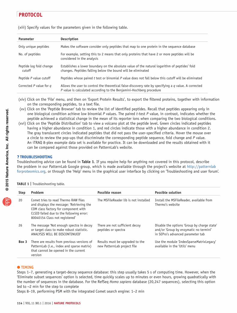
(xiii) Specify values for the parameters given in the following table.

parameter Description

Only unique peptides Makes the software consider only peptides that map to one protein in the sequence database

No. of peptides For example, setting this to 2 means that only proteins that have 2 or more peptides will be considered in the analysis

Peptide log fold change cutoff

Establishes a lower boundary on the absolute value of the natural logarithm of peptides’ fold changes. Peptides falling below the bound will be eliminated

Peptide P value cutoff Peptides whose paired t test or binomial P value does not fall below this cutoff will be eliminated

Corrected P value for q Allows the user to control the theoretical false-discovery rate by specifying a q value. A corrected P value is calculated according to the Benjamini-Hochberg procedure

(xiv) Click on the ‘File’ menu, and then on ‘Export Protein Results’, to export the filtered proteins, together with information on the corresponding peptides, to a text file.

(xv) Click on the ‘Peptide Browser’ tab to review the list of identified peptides. Recall that peptides appearing only in one biological condition achieve low binomial P values. The paired t-test P value, in contrast, indicates whether the peptide achieved a statistical change in the mean of its reporter ions when comparing the two biological conditions.

(xvi) Click on the ‘Peptide Distribution’ tab to view a volcano plot at the peptide level. Green circles indicated peptides having a higher abundance in condition 1, and red circles indicate those with a higher abundance in condition 2. The gray translucent circles indicated peptides that did not pass the user-specified criteria. Hover the mouse over a circle to review the pop-ups that discriminate the corresponding peptide sequence, fold change and P value. An iTRAQ 8-plex example data set is available for practice. It can be downloaded and the results obtained with it can be compared against those provided on PatternLab’s website.

? trouBlesHootInGTroubleshooting advice can be found in table 1. If you require help for anything not covered in this protocol, describe the problem in our PatternLab Google group, which is made available through the project’s website at http://patternlab forproteomics.org, or through the ‘Help’ menu in the graphical user interface by clicking on ‘Troubleshooting and user forum’.

● tIMInGSteps 1–7, generating a target-decoy sequence database: this step usually takes 5 s of computing time. However, when the ‘Eliminate subset sequences’ option is selected, time quickly scales up to minutes or even hours, growing quadratically with the number of sequences in the database. For the RefSeq Homo sapiens database (20,247 sequences), selecting this option led to ~2 min for the step to completeSteps 8–19, performing PSM with the integrated Comet search engine: 1–2 min

taBle 1 | Troubleshooting table.

step problem possible reason possible solution

20 Comet tries to read Thermo RAW files and displays the message: ‘Retrieving the COM class factory for component with CLSID failed due to the following error: 80040154 Class not registered’

The MSFileReader lib is not installed Install the MSFileReader, available from Thermo’s website

26 The message ‘Not enough spectra in decoy or target class to make robust statistic. ANALYSIS WILL BE DISCONTINUED’

There are not sufficient decoy peptides or spectra

Disable the options ‘Group by charge state’ and/or ‘Group by enzymatic no termini’ in SEPro’s advanced parameter tab

Box 3 There are results from previous versions of PatternLab (i.e., index and sparse matrix) that cannot be opened in the current version

Results must be upgraded to the new PatternLab project file

Use the module ‘IndexSparseMatrixLegacy’ available in the ‘Utils’ menu

©20

15N

atu

re A

mer

ica,

Inc.

All

rig

hts

res

erve

d.

protocol

nature protocols | VOL.11 NO.1 | 2016 | 115

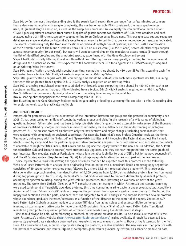
Step 20, by far, the most time-demanding step is the search itself: search time can range from a few minutes up to more than a day, varying mostly with sample complexity, the number of variable PTMs considered, the mass spectrometer used, LC gradient length and so on, as well as the computer’s processor. We exemplify the computational burden of an iTRAQ 8-plex experiment obtained from human biopsies of gastric cancer; two fractions of HILIC were obtained and each analyzed using a 2-h RP chromatography coupled online to an Obritrap Velos instrument. This example data set and sequence database are made available on PatternLab’s website as an exercise to certify that one can reproduce our results as indicated. The search, considering only the fixed modifications of carbamidomethylation of cysteine, and the iTRAQ 8 modification at the N terminus and at the K and Y residues, took 1,035 s on our 24-core (2 × X5675 Xeon) server. All other steps happen almost instantaneously (30 s at most), but users will want to spend time on the modules to assess results (browse through the list of identified proteins and the annotated spectra, experiment with the Gene Ontology and so on)Steps 21–29, statistically filtering Comet results with SEPro: filtering time can vary greatly according to the experimental design and the number of spectra. It is expected to fall somewhere near 30 s for a typical 2-h LC-MS/MS analysis acquired on an Orbitrap Velos instrumentStep 30A, quantification analysis with spectral counting: computing time should be ~20 s per SEPro file, assuming each file originated from a typical 2-h LC-MS/MS analysis acquired on an Orbitrap VelosStep 30B, quantification analysis with XIC: computing time should be ~30–40 s for each mass spectrum raw file, assuming that each file originated from a typical 2-h LC-MS/MS analysis acquired on an Orbitrap VelosStep 30C, analyzing multiplexed experiments labeled with isobaric tags: computing time should be ~20–50 s for each mass spectrum raw file, assuming that each file originated from a typical 2-h LC-MS/MS analysis acquired on an Orbitrap VelosBox 3, differential proteomics: typically takes <3 s of computing time for any of the modulesBox 4, scoring phosphopeptides: the overall computing time is ~35 sBox 5, setting up the Gene Ontology Explorer module: generating or loading a .precomp file can take ~5 min. Computing time for exploring one’s data is practically negligible

antIcIpateD resultsPatternLab for proteomics 4.0 is the culmination of the interaction between our group and the proteomics community since 2008. It has been tested on millions of spectra by various groups and aided in the research of a wide range of biological questions. Indeed, PatternLab’s goal has been to help scientists identify, quantify and attempt to make sense of the thousands of proteins identified by shotgun proteomics in order to ultimately make a difference in the understanding of biological processes61,62. The present protocol emphasizes only the new features and major changes, including some modules that were replaced with completely re-designed substitutes. For example, PatternLab’s new Project Organizer replaces the former ‘Regrouper’, doing away with the ‘index.txt’ and ‘SparseMatrix.txt’ files and introducing the PatternLab project file instead, which is used by many modules for performing quantitative proteomic analyses. The current version also includes a tool, which is accessible through the ‘Utils’ menu, that allows one to upgrade the legacy format to the new one. In addition, the SEProQ functionalities (XIC and Isobaric browser) were substantially upgraded, and they are now integrated into the same graphical user interface. New modules, such as PepExplorer, whose functionality is similar to that of SEPro but for de novo sequencing33, and the XD Scoring system (supplementary Fig. 6) for phosphopeptide localization, are also part of the new version.

Some representative works illustrating the types of results that can be expected from this protocol are the following. Webb et al. used PatternLab to analyze data originating from an online two-dimensional liquid chromatography separation consisting of 39 strong cation-exchange steps followed by a short 18.5-min reversed-phase gradient63. This large-scale data generation approach enabled the identification of 4,269 proteins from 4,189 distinguishable protein families from yeast during log phase growth. In this study, PatternLab’s T-Fold module was used to pinpoint differentially abundant proteins, according to spectral counting, during the yeast cellular quiescence, thus providing an overview of most of the yeast proteome. The works from Christie-Oleza et al.64,65 constitute another example in which PatternLab and spectral counting were used to pinpoint differentially abundant proteins, this time comparing marine bacteria under several natural conditions. Aquino et al.5 used PatternLab’s XIC module to explore the proteomic landscape of a gastric tumor biopsy. In the latter, the biopsy was sectioned into ten parts, and each part was subjected to MudPIT analysis; the authors identified several proteins whose abundance gradually increases/decreases as a function of the distance to the center of the tumor. Chaves et al.66 used PatternLab’s Isobaric analyzer module to analyze TMT data from aging soleus and extensor digitorum longus rat muscles, disclosing quantitative data for more than 4,000 proteins. Finally, Shah et al.67 used PatternLab’s TrendQuest module to group protein expression profiles of Jatropha curcas seeds during five developmental stages.

One should always be able, when following a protocol, to reproduce previous results. To help make sure that this is the case, PatternLab’s project website (http://www.patternlabforproteomics.org) makes available, through its download tab, previously analyzed data sets whose download and re-analysis we recommend strongly to those using PatternLab for the first time. All intermediate files, acquired step by step along the protocol, are also available. The new user can then practice with the protocol to reproduce our results. Figure 9 exemplifies good results provided by PatternLab’s Isobaric module on data

©20

15N

atu

re A

mer

ica,

Inc.

All

rig

hts

res

erve

d.

protocol

116 | VOL.11 NO.1 | 2016 | nature protocols

acquired using the MultiNotch approach on TMT-labeled peptides analyzed us-ing an Orbitrap Fusion (Thermo, San Jose). This is so because peptides (dots) are evenly distributed along the y-axis and assume a disposition similar to the eruption of a volcano, thus constituting a so-called volcano plot.

As with any software pipeline or even individual scientist, it is the feedback from collaborators and other peers that drives improvement. In the case of PatternLab, all the feedback, suggestions and even bug fixes have been the most important assets we could count on, helping our suite of tools become more and more sophisticated and hopefully ever closer to supporting answers to questions that were previously intangible. In this regard, we look forward to receiving user feedback through the newly created forum so we can continue to improve on this community-driven and freely available tool.

Figure 9 | PatternLab’s Isobaric Analyzer. The screenshot shows the result of an analysis. Each dot represents a peptide that is mapped according to its log fold change (y-axis) and its differential abundance P value (x-axis). Peptides colored in green or red are those that satisfied user-specified cutoff criteria for fold-change and P value.

Note: Any Supplementary Information and Source Data files are available in the online version of the paper.

acknowleDGMents We thank Conselho Nacional de Desenvolvimento Científico e Tecnológico (CNPq), Fundação do Câncer, Fundação de Amparo à Pesquisa do Estado do Rio de Janeiro (FAPERJ) for its BBP grant and Programa de Apoio à Pesquisa Estratégica em Saúde da Fiocruz (PAPES VII). J.R.Y. acknowledges funding from the US National Institutes of Health (P41 GM103533, R01 MH067880, and R01 MH100175) and the National Heart, Lung and Blood Institute (NHBLI) Proteomics Center at the University of California at Los Angeles (UCLA) (HHSN268201000035C). J.J.M. acknowledges NIH research resources (5P41RR011823) and funding from the National Institute of General Medical Sciences (8 P41 GM103533).

autHor contrIButIons P.C.C., J.R.Y. and V.C.B. have participated in the PatternLab project since its beginning in 2008. D.B.L. participated in updating features from several modules and the graphical user interface, as well as in helping migrate to the new PatternLab project file format. F.V.L. developed the PepExplorer module together with P.C.C. M.D.M.S. developed several functions in PepExplorer and had a major participation in the development of the isobaric quantification module. J.S.G.F., P.F.A. and J.J.M. have been participating in PatternLab since early versions by continuously performing beta testing, pointing out required features and providing suggestions on how to make the software more user-friendly. P.C.C. and D.B.L. created the supplementary video. P.C.C. and V.C.B. wrote the manuscript. All authors read and approved the manuscript.

coMpetInG FInancIal Interests The authors declare no competing financial interests.

Reprints and permissions information is available online at http://www.nature.com/reprints/index.html.

1. Hebert, A.S. et al. The one-hour yeast proteome. Mol. Cell. Proteomics 13, 339–347 (2014).

2. Yates, J.R. Mass spectrometry and the age of the proteome. J. Mass Spectrom. 33, 1–19 (1998).

3. Zhang, B., Chambers, M.C. & Tabb, D.L. Proteomic parsimony through bipartite graph analysis improves accuracy and transparency. J. Proteome Res. 6, 3549–3557 (2007).

4. Hwang, S.-I. et al. Systematic characterization of nuclear proteome during apoptosis: a quantitative proteomic study by differential extraction and stable isotope labeling. Mol. Cell. Proteomics 5, 1131–1145 (2006).

5. Aquino, P.F. et al. Exploring the proteomic landscape of a gastric cancer biopsy with the shotgun imaging analyzer. J. Proteome Res. 13, 314–320 (2014).

6. Calvete, J.J., Sanz, L., Angulo, Y., Lomonte, B. & Gutiérrez, J.M. Venoms, venomics, antivenomics. FEBS Lett. 583, 1736–1743 (2009).

7. Valente, R.H., Dragulev, B., Perales, J., Fox, J.W. & Domont, G.B. BJ46a, a snake venom metalloproteinase inhibitor. Isolation, characterization, cloning and insights into its mechanism of action. Eur. J. Biochem 268, 3042–3052 (2001).

8. Eng, J.K., McCormack, A.L. & Yates, J.R. An approach to correlate tandem mass spectral data of peptides with amino acid sequences in a protein database. J. Am. Soc. Mass Spectrom. 5, 976–989 (1994).

9. Washburn, M.P., Wolters, D. & Yates, J.R. III. Large-scale analysis of the yeast proteome by multidimensional protein identification technology. Nat. Biotechnol. 19, 242–247 (2001).

10. Köcher, T., Pichler, P., Swart, R. & Mechtler, K. Analysis of protein mixtures from whole-cell extracts by single-run nanoLC-MS/MS using ultralong gradients. Nat. Protoc. 7, 882–890 (2012).

11. Keller, A., Nesvizhskii, A.I., Kolker, E. & Aebersold, R. Empirical statistical model to estimate the accuracy of peptide identifications made by MS/MS and database search. Anal. Chem. 74, 5383–5392 (2002).

12. Cociorva, D., L Tabb, D. & Yates, J.R. Validation of tandem mass spectrometry database search results using DTASelect. Curr. Protoc. Bioinformatics 16 74, 13.4.1–13.4.14 (2007).

13. Ross, P.L. et al. Multiplexed protein quantitation in Saccharomyces cerevisiae using amine-reactive isobaric tagging reagents. Mol. Cell. Proteomics 3, 1154–1169 (2004).

14. Oda, Y., Huang, K., Cross, F.R., Cowburn, D. & Chait, B.T. Accurate quantitation of protein expression and site-specific phosphorylation. Proc. Natl. Acad. Sci. USA 96, 6591–6596 (1999).

15. Carvalho, P.C., Hewel, J., Barbosa, V.C. & Yates, J.R. III. Identifying differences in protein expression levels by spectral counting and feature selection. Genet. Mol. Res. 7, 342–356 (2008).

16. Liu, H., Sadygov, R.G. & Yates, J.R. III. A model for random sampling and estimation of relative protein abundance in shotgun proteomics. Anal. Chem. 76, 4193–4201 (2004).

17. Neilson, K.A. et al. Less label, more free: approaches in label-free quantitative mass spectrometry. Proteomics 11, 535–553 (2011).

18. Shevchenko, A., Valcu, C.-M. & Junqueira, M. Tools for exploring the proteomosphere. J. Proteomics 72, 137–144 (2009).

19. Beausoleil, S.A., Villén, J., Gerber, S.A., Rush, J. & Gygi, S.P. A probability-based approach for high-throughput protein phosphorylation analysis and site localization. Nat. Biotechnol. 24, 1285–1292 (2006).

©20

15N

atu

re A

mer

ica,

Inc.

All

rig

hts

res

erve

d.

protocol

nature protocols | VOL.11 NO.1 | 2016 | 117

20. Carvalho, P.C. et al. YADA: a tool for taking the most out of high-resolution spectra. Bioinformatics 25, 2734–2736 (2009).

21. Keller, A., Eng, J., Zhang, N., Li, X. & Aebersold, R. A uniform proteomics MS/MS analysis platform utilizing open XML file formats. Mol. Syst. Biol. 1, 2005.0017 (2005).

22. Deutsch, E.W. et al. Trans-Proteomic Pipeline, a standardized data processing pipeline for large-scale reproducible proteomics informatics. Proteomics Clin. Appl. 9, 745–754 (2015).

23. Kohlbacher, O. et al. TOPP–the OpenMS proteomics pipeline. Bioinformatics 23, e191–e197 (2007).

24. Cox, J. & Mann, M. MaxQuant enables high peptide identification rates, individualized p.p.b.-range mass accuracies and proteome-wide protein quantification. Nat. Biotechnol. 26, 1367–1372 (2008).

25. Cox, J. et al. A practical guide to the MaxQuant computational platform for SILAC-based quantitative proteomics. Nat. Protoc. 4, 698–705 (2009).

26. Carvalho, P.C., Fischer, J.S.G., Chen, E.I., Yates, J.R. & Barbosa, V.C. PatternLab for proteomics: a tool for differential shotgun proteomics. BMC Bioinformatics 9, 316 (2008).

27. MacLean, B. et al. Skyline: an open source document editor for creating and analyzing targeted proteomics experiments. Bioinformatics 26, 966–968 (2010).

28. Giardine, B. et al. Galaxy: a platform for interactive large-scale genome analysis. Genome Res. 15, 1451–1455 (2005).

29. Boekel, J. et al. Multi-omic data analysis using Galaxy. Nat. Biotechnol. 33, 137–139 (2015).

30. Egertson, J.D., MacLean, B., Johnson, R., Xuan, Y. & MacCoss, M.J. Multiplexed peptide analysis using data-independent acquisition and Skyline. Nat. Protoc. 10, 887–903 (2015).

31. Carvalho, P.C., Yates, J.R. III. & Barbosa, V.C. Improving the TFold test for differential shotgun proteomics. Bioinformatics 28, 1652–1654 (2012).

32. Leprevost, F.V. et al. Pinpointing differentially expressed domains in complex protein mixtures with the cloud service of PatternLab for Proteomics. J. Proteomics 89, 179–182 (2013).

33. Leprevost, F.V. et al. PepExplorer: A similarity-driven tool for analyzing de novo sequencing results. Mol. Cell. Proteomics 13, 2480–2489 (2014).

34. Fischer, J. et al. A scoring model for phosphopeptide site localization and its impact on the question of whether to use MSA. J. Proteomics 129, 42–50 (2015).

35. Fischer, J. et al. Dynamic proteomic overview of glioblastoma cells (A172) exposed to perillyl alcohol. J. Proteomics 73, 1018–1027 (2010).

36. Carvalho, P.C. et al. GO Explorer: a gene-ontology tool to aid in the interpretation of shotgun proteomics data. Proteome Sci. 7, 6 (2009).

37. Lima, D.B. et al. SIM-XL: a powerful and user-friendly tool for peptide cross-linking analysis. J. Proteomics 129, 51–55 (2015).

38. Borges, D. et al. Using SIM-XL to identify and annotate cross-linked peptides analyzed by mass spectrometry. Protoc. Exch. doi:10.1038/protex.2015.015 (2015).

39. Carvalho, P.C., Yates Iii, J.R. & Barbosa, V.C. Analyzing shotgun proteomic data with PatternLab for proteomics. Curr. Protoc. Bioinformatics 30, 13.13.1–13.13.15 (2010).

40. Carvalho, P.C. et al. Search engine processor: filtering and organizing peptide spectrum matches. Proteomics 12, 944–949 (2012).

41. Carvalho, P.C., Fischer, J.S.G., Xu, T., Yates, J.R. III. & Barbosa, V.C. PatternLab: from mass spectra to label-free differential shotgun proteomics. Curr. Protoc. Bioinformatics 40, 13.19.1–13.19.18 (2012).

42. Eng, J.K., Jahan, T.A. & Hoopmann, M.R. Comet: an open-source MS/MS sequence database search tool. Proteomics 13, 22–24 (2013).

43. Richards, A.L. et al. One-hour proteome analysis in yeast. Nat. Protoc. 10, 701–714 (2015).

44. UniProt Consortium. Update on activities at the Universal Protein Resource (UniProt) in 2013. Nucleic Acids Res. 41, D43–D47 (2013).

45. Elias, J.E. & Gygi, S.P. Target-decoy search strategy for increased confidence in large-scale protein identifications by mass spectrometry. Nat. Methods 4, 207–214 (2007).

46. Cottrell, J.S. & Creasy, D.M. Response to: the problem with peptide presumption and low mascot scoring. J. Proteome Res. 10, 5272–5273 (2011).

47. Bandeira, N. Spectral networks: a new approach to de novo discovery of protein sequences and posttranslational modifications. BioTechniques 42 687 (2007).

48. Na, S., Bandeira, N. & Paek, E. Fast multi-blind modification search through tandem mass spectrometry. Mol. Cell. Proteomics 11, M111.010199 (2012).

49. Shevchenko, A. et al. Charting the proteomes of organisms with unsequenced genomes by MALDI-quadrupole time-of-flight mass spectrometry and BLAST homology searching. Anal. Chem. 73, 1917–1926 (2001).

50. Xu, T. et al. ProLuCID, a fast and sensitive tandem mass spectra-based protein identification program. Mol. Cell Proteomics 5, S174 (2006).

51. Borges, D. et al. Effectively addressing complex proteomic search spaces with peptide spectrum matching. Bioinformatics 29, 1343–1344 (2013).

52. Zybailov, B. et al. Statistical analysis of membrane proteome expression changes in Saccharomyces cerevisiae. J. Proteome Res. 5, 2339–2347 (2006).

53. Thompson, A. et al. Tandem mass tags: a novel quantification strategy for comparative analysis of complex protein mixtures by MS/MS. Anal. Chem. 75, 1895–1904 (2003).

54. McAlister, G.C. et al. MultiNotch MS3 enables accurate, sensitive, and multiplexed detection of differential expression across cancer cell line proteomes. Anal. Chem. 86, 7150–7158 (2014).

55. Picotti, P. & Aebersold, R. Selected reaction monitoring-based proteomics: workflows, potential, pitfalls and future directions. Nat. Methods 9, 555–566 (2012).

56. Vizcaíno, J.A. et al. The PRoteomics IDEntifications (PRIDE) database and associated tools: status in 2013. Nucleic Acids Res. 41, D1063–D1069 (2013).

57. Chambers, M.C. et al. A cross-platform toolkit for mass spectrometry and proteomics. Nat. Biotechnol. 30, 918–920 (2012).

58. Martens, L. et al. mzML–a community standard for mass spectrometry data. Mol. Cell. Proteomics 10, R110.000133 (2011).

59. McDonald, W.H. et al. MS1, MS2, and SQT-three unified, compact, and easily parsed file formats for the storage of shotgun proteomic spectra and identifications. Rapid Commun. Mass Spectrom. 18, 2162–2168 (2004).

60. Nesvizhskii, A.I. Proteogenomics: concepts, applications and computational strategies. Nat. Methods 11, 1114–1125 (2014).

61. de Miguel, N. et al. Proteome analysis of the surface of Trichomonas vaginalis reveals novel proteins and strain-dependent differential expression. Mol. Cell. Proteomics 9, 1554–1566 (2010).

62. Clair, G., Armengaud, J. & Duport, C. Restricting fermentative potential by proteome remodeling: an adaptive strategy evidenced in Bacillus cereus. Mol. Cell. Proteomics 11, M111.013102 (2012).

63. Webb, K.J., Xu, T., Park, S.K. & Yates, J.R. Modified MuDPIT separation identified 4488 proteins in a system-wide analysis of quiescence in yeast. J. Proteome Res. 12, 2177–2184 (2013).

64. Christie-Oleza, J.A., Piña-Villalonga, J.M., Bosch, R., Nogales, B. & Armengaud, J. Comparative proteogenomics of twelve Roseobacter exoproteomes reveals different adaptive strategies among these marine bacteria. Mol. Cell. Proteomics 11, M111.013110 (2012).

65. Christie-Oleza, J.A., Fernandez, B., Nogales, B., Bosch, R. & Armengaud, J. Proteomic insights into the lifestyle of an environmentally relevant marine bacterium. ISME J. 6, 124–135 (2012).

66. Chaves, D.F.S. et al. Comparative proteomic analysis of the aging soleus and extensor digitorum longus rat muscles using TMT labeling and mass spectrometry. J. Proteome Res. 12, 4532–4546 (2013).

67. Shah, M. et al. Proteomic analysis of the endosperm ontogeny of Jatropha curcas L. seeds. J. Proteome Res. 14, 2557–2568 (2015).