Integer programming formulations for the elementaryshortest path problem

Leonardo TaccariDipartimento di Elettronica, Informazione e Bioingegneria, Politecnico di Milano, Italy

Abstract

Given a directed graph G = (V,A) with arbitrary arc costs, the ElementaryShortest Path Problem (ESPP) consists of finding a minimum-cost path be-tween two nodes s and t such that each node of G is visited at most once. Ifnegative costs are allowed, the problem is NP-hard. In this paper, several inte-ger programming formulations for the ESPP are compared. We present analyt-ical results based on a polyhedral study of the formulations, and computationalexperiments where we compare their linear programming relaxation bounds andtheir behavior within a branch-and-cut framework. The computational resultsshow that a formulation with dynamically generated cutset inequalities is themost effective.Keywords: integer programming, elementary shortest path, branch-and-cut,extended formulations, subtour elimination constraints, generalized cutsetinequalities

1. Introduction

Given a directed graph G = (V,A) and arc costs cij for each (i, j) ∈ A,the shortest path problem consists of finding a minimum-cost path between twonodes s and t.

Often, an implicit assumption is that such path has to be elementary. Apath is elementary if it does not visit any node more than once, i.e., if it doesnot contain subtours. When the costs cij induce no negative cycles on G, theproblem can be solved efficiently via ad-hoc polynomial time algorithms, likeBellman-Ford’s or Dijikstra’s algorithm (if cij ≥ 0). However, if negative cy-cles do arise, subtours must be explicitly prevented, leading to the so-calledElementary Shortest Path Problem (ESPP).

The ESPP is clearly NP-hard due to a simple reduction from the Hamilto-nian path problem. Its equivalent maximization counterpart, where one seeks alongest path over a graph with positive cycles, has been vastly discussed in the

Email address: leonardo.taccari@polimi.it (Leonardo Taccari)

Preprint submitted to Elsevier December 21, 2015

literature, usually referred to as the Longest Path Problem (LPP). Björklund etal. [7] prove that the LPP is hard to approximate on unweighted directed graphswithin a n1−ε for any ε, unless P = NP. For undirected graphs, approximationalgorithms are described in, e.g., [27] and [17].

Related to the ESPP are variants of the Travelling Salesman Problem (TSP)with profits, such as the Prize Collecting TSP [3], the Orienteering Problem [36]and the Capacitated Profitable Tour Problem [26], that involve prizes on eachnode, which can be visited at most once.

While an interesting problem in its own right, the ESPP also arises in thepricing subproblems of branch-and-price algorithms [1]. Often, the pricing phasein Vehicle Routing Problems (VRP) involves resource-constrained variants of theelementary shortest path problem (ESPPRC) [23]. These problems are usuallysolved with fast dynamic programming-based label algorithms, e.g., see [32, 15,8]. It is possible to adapt this kind of approach to the unconstrained ESPP byconsidering an artificial resource for each node which is consumed when the nodeis visited, and imposing that no more than one unit of each resource is used, asalready proposed in [6, 8]. However, this is a rather weak constraint, in the sensethat it allows for very long paths, so that approaches based on label algorithmsbecome very time consuming, as noted by Drexl and Irnich [14]. This limitationis already highlighted for the ESPP with a capacity constraint by Jepsen etal. [25], that propose a branch-and-cut algorithm that significantly outperformslabel algorithms. In the context of a branch-and-price algorithm, where theESPP is solved repeatedly in the pricing phase, another desirable feature ofan integer programming approach is its flexibility, that allows one to easilyincorporate general branching decisions or valid inequalities (e.g., the subset-rowinequalities in [24]) that would change the structure of the pricing subproblem.These reasons motivate the study of integer programming techniques for theESPP.

Several branch-and-cut approaches can be found in the literature for relatedproblems [5, 19, 16, 26]. However, not much previous work has appeared oninteger programming approaches tailored specifically for the ESPP. Ibrahim etal. [22] provide computational results on the linear programming (LP) boundsof a flow-based extended formulation, but give no details on its behavior ina branch-and-bound algorithm. Another extended formulation is proposed byHaouari et al. [21]. Drexl and Irnich [14] describe a branch-and-cut approachand compare its efficiency with the extended formulation in [22], while Drexl [13]studies the efficient separation of subtour elimination constraints for the ESPP.

In the context of integer programming, the choice of a formulation is crucialfor the effectiveness of methods based on branch-and-cut. In this article wepresent a thorough comparison between different formulations for the ESPP,which are described in detail in Section 2. We include integer programming for-mulations with exponentially many subtour elimination constraints, and mixed-integer programming extended formulations with a polynomial number of vari-ables and constraints. In Section 3 we provide some analytical results, includinga proof of equivalence between the polyhedra described by the two strongest for-mulations. Section 4 reports computational experiments where we compare the

2

LP relaxation bounds and branch-and-cut results. Finally, in Section 5, we givesome concluding remarks and discuss further research topics.

2. Integer programming formulations

Let us consider a directed graph G = (V,A) with the set of nodes V and theset of arcs A. Let n and m be the cardinality of V and A, respectively. A pathis a sequence of nodes v1, . . . , vk, and is said to be elementary if no node appearsin the path more than once. A cycle, or tour, is a path with v1 = vk. We denoteby δ+(i) and δ−(i) the set of outgoing and incoming arcs of node i, by δ+(S)and δ−(S) the arcs leaving/entering the set S ⊆ V , and by A(S) the set of arcswith both ends in S ⊆ V . Let us also define Vi := V \{i}, Vij := V \{i, j}, and,for any arc set B ⊆ A, we define x(B) :=

∑b∈B xb. In all the formulations, it

is assumed w.l.o.g. that |δ−(s)| = |δ+(t)| = 0.A standard integer programming formulation to determine a shortest path

from node s to node t is the following:

min∑

(i,j)∈A

cijxij (1)

∑(i,j)∈δ+(i)

xij −∑

(j,i)∈δ−(i)

xji =

1 if i = s

−1 if i = t

0 else∀i ∈ V (2)

∑(i,j)∈δ+(i)

xij ≤ 1 ∀i ∈ V (3)

xij ∈ {0, 1} ∀(i, j) ∈ A, (4)

where cij ∈ R are the arc costs, and xij are binary arc variables that take value1 if the arc (i, j) belongs to the path. Constraints (2) are flow conservationconstraints, while Constraints (3) ensure that the outgoing degree of each nodeis at most one. When the costs cij induce negative cycles on G, i.e., there is asubtour such that the total cost of its arcs is negative, this system of inequalitiesis not sufficient to guarantee the elementarity of the path. Thus, additionalconstraints (and possibly variables) are necessary to prevent subtours.

Notice that the crucial difference with respect to problems in which the pathhas to be Hamiltonian is the absence of the degree constraints:∑

(i,j)∈δ+(i)

xij =∑

(j,i)∈δ−(i)

xji = 1 ∀i ∈ Vst.

We now describe different sets of constraints and variables that can be addedto Formulation (1)–(4) to obtain a valid integer programming formulation forthe ESPP.

3

2.1. Dantzig-Fulkerson-Johnson (DFJ)For the TSP, success has been achieved with strong formulations with ex-

ponentially many constraints. It is possible to write a formulation for theESPP based on the classical Dantzig-Fulkerson-Johnson subtour eliminationconstraints [10], adding to the basic formulation (1)–(4) the following inequali-ties: ∑

(i,j)∈A(S)

xij ≤ |S| − 1 ∀S ⊆ Vst, |S| ≥ 2. (5)

In each subset S, subtours are prevented ensuring that the number of arcs in Swhich are selected is smaller than the number of nodes in S. This formulationincludes O(m) variables and O(2n) constraints.

Observation. For Hamiltonian path problems, due to the degree constraints, theDFJ subtour eliminations constraints can be equivalently written in the cutsetform: ∑

(i,j)∈δ+(S)

xij ≥ 1 ∀S ⊂ V, |S| ≥ 2. (6)

For the ESPP, Constraints (6) are valid only for subsets S with s ∈ S andt /∈ S. Moreover, they are not sufficient to prevent all subtours.

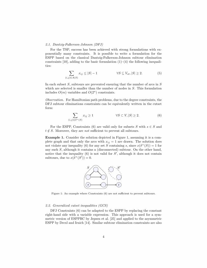
Example 1. Consider the solution depicted in Figure 1, assuming it is a com-plete graph and that only the arcs with xij = 1 are drawn. The solution doesnot violate any inequality (6) for any set S containing s, since x(δ+(S)) = 1 forany such S, although it contains a (disconnected) subtour. On the other hand,notice that the inequality (6) is not valid for S′, although it does not containsubtours, due to x(δ+(S′)) = 0.

S S′

s t

Figure 1: An example where Constraints (6) are not sufficient to prevent subtours.

2.2. Generalized cutset inequalities (GCS)DFJ Constraints (6) can be adapted to the ESPP by replacing the constant

right-hand side with a variable expression. This approach is used for a sym-metric version of ESPPRC by Jepsen et al. [25] and applied to the asymmetricESPP by Drexl and Irnich [14]. Similar subtour elimination constraints are also

4

used in branch-and-cut algorithms for the VRP [29] or variants of the TSP withprofits [16, 26]. We refer to them as generalized cutset inequalities (GCS):∑

(i,j)∈δ+(S)

xij ≥∑

(k,j)∈δ+(k)

xkj∀k ∈ S, ∀S ⊆ Vst,

|S| ≥ 2. (7)

Constraints (7) prevent subtours by ensuring that, for each subset S, the numberof selected arcs leaving S is not smaller than the number of selected arcs outgoingfrom any node in S. In an integer solution, this means that the cut inducedby S must contain at least one arc if at least one node in S belongs to the s-tpath, while, if S does not contain any node in the s-t path, the constraint is thetrivial inequality. The number of variables in the formulation is O(m), whilethe number of constraints is O(n2n).

Constraints (7) can be shown to be equivalent to a strengthened version of(5).

Proposition 2. Constraints (7) can be rewritten as:∑(i,j)∈A(S)

xij ≤∑

i∈S\{k}

∑(i,j)∈δ+(i)

xij∀k ∈ S, ∀S ⊆ Vst,

|S| ≥ 2. (8)

Proof. For all k ∈ S, x(δ+(k)) ≤ x(δ+(S)) = x(δ+(S)) + x(A(S))− x(A(S)) =∑i∈S x(δ+(i))− x(A(S)).

These inequalities can be interpreted as imposing that the number of selectedarcs in a subset S is strictly smaller than the number of nodes in S that belongto the s-t path.

2.3. Sequential formulation (MTZ)To derive an extended formulation à la Miller, Tucker and Zemlin [28] (here-

after MTZ) it is enough to introduce, for each node, an auxiliary variable thatcan be viewed as the position of the node along the path and a constraint foreach arc:

tj ≥ ti + 1 + (n− 1)(xij − 1) ∀(i, j) ∈ A,i 6= s, j 6= t.

(9)

For the Asymmetric TSP (ATSP), this formulation is well-known to give poorlinear relaxation bounds. However, it is very compact, as it requires only O(m)additional constraints and O(n) auxiliary variables.

2.4. Reformulation-linearization based formulation (RLT)From the following nonlinear reformulation of the MTZ formulation:

tjxij = (ti + 1)xij ∀(i, j) ∈ A, i 6= s (10)tjxsj = xsj ∀(s, j) ∈ δ+(s) (11)1 ≤ ti ≤ n− 1, i ∈ Vs (12)

5

Haouari et al. [21] apply a partial Sherali-Adams reformulation-linearizationtechnique [33] to obtain the following stronger formulation for the ESPP:

αij = βij + xij ∀(i, j) ∈ A (13)

xsj +∑

(i,j)∈δ−(j)i 6=s

αij −∑

(j,i)∈δ+(j)

βji = 0 ∀j ∈ Vt,(s, j) ∈ δ+(s) (14)

∑(i,j)∈δ−(j)

αij −∑

(j,i)∈δ+(j)

βji = 0 ∀j ∈ Vst,(s, j) /∈ δ+(s) (15)

αij ≤ (n− 1)xij ∀(i, j) ∈ A, i 6= s (16)xij ≤ βij ∀(i, j) ∈ A, i 6= s (17)αij ≥ 0, βij ≥ 0 ∀(i, j) ∈ A, (18)

where the bilinear terms are linearized introducing the variables αij := tjxij andβij := tixij and Constraints (16)–(17). On a given selected arc (i, j) ∈ A, thevariables βij and αij can be interpreted respectively as the position of the nodesi and j along the path. This extended formulation requires O(m) constraintsand O(m) auxiliary variables.

2.5. Single-flow formulation (SF)A formulation similar to the single-flow ATSP formulation of Gavish and

Graves [18] can be obtained introducing an auxiliary flow q to be delivered tothe nodes belonging to the s-t path. In addition, variables zk are added to theformulation:

qij ≤ (n− 1)xij ∀(i, j) ∈ A (19)∑(s,j)∈δ+(s)

qsj =∑k∈Vs

zk (20)

∑(i,k)∈δ−(k)

qik −∑

(k,j)∈δ+(k)

qkj = zk ∀k ∈ Vs (21)

∑(i,k)∈δ−(k)

xik = zk ∀k ∈ Vs (22)

qij ≥ 0 ∀(i, j) ∈ A (23)zk ∈ {0, 1} ∀k ∈ Vs. (24)

Constraints (19) impose that the auxiliary flow is positive only over the arcswhere xij = 1. The auxiliary flow leaving from the node s has value equalto the number of nodes that are reached by the s-t path. Constraints (21)ensure that the balance of the auxiliary flow on each node is equivalent to zk,which, according to Constraint (22), is either 1, if node k is in the s-t path, or0 otherwise.

6

2.6. Multicommodity-flow formulation (MCF)An extension of the single-flow formulation is obtained by disaggregating the

auxiliary flow into n− 1 unitary flows. Subtours are prevented by enforcing oneunit of a distinct auxiliary flow from s to each node that belongs to the s-t path:

qkij ≤ xij∀k ∈ Vs,

(i, j) ∈ A (25)

∑(i,j)∈δ+(i)

qkij −∑

(j,i)∈δ−(i)

qkji =

zk if i = s

−zk if i = k

0 else

∀i ∈ V,∀k ∈ Vs

(26)

∑(i,k)∈δ−(k)

xik = zk ∀k ∈ Vs (27)

∑(s,j)∈δ+(s)

xsj = 1 (28)

∑(i,t)∈δ−(t)

xit = 1 (29)

qkij ≥ 0 ∀k ∈ Vs,(i, j) ∈ A (30)

zk ∈ {0, 1} ∀k ∈ Vs. (31)

The formulation includes O(nm) additional variables and constraints. Thisextended formulation is introduced, for the ESPP, by Ibrahim et al. [22], andit is very similar to classic multi-commodity flow formulations for the ATSPproposed by Wong [37] and Claus [9].

2.7. OverviewIn Table 1 we summarize the presented formulations. To the best of our

knowledge, formulations MTZ and SF have not been previously considered forthe ESPP, although similar ones are well known for TSP or VRP variants.

Table 1: A summary of the considered formulations.

number ofvariables constraints description

DFJ O(m) O(2n) Dantzig-Fulkerson-Johnson (5)GCS O(m) O(n2n) generalized cutsets (7)MTZ O(m) O(m) Miller-Tucker-Zemlin (9)RLT O(m) O(m) reformulation-linearization (13)–(18)SF O(m) O(m) single-flow (19)-(24)

MCF O(nm) O(nm) multi-commodity flow (25)-(31)

7

3. Polyhedral results

Let us describe some analytical results for the considered ESPP formulations.

Proposition 3. Formulation MCF is stronger than formulation SF.

Proof. Constraints (19)–(21) can be obtained from MCF simply aggregatingConstraints (25)–(26) over k ∈ Vs, and then substituting

∑k∈Vs

qkij with qij .The example in Figure 2 shows that the inclusion is strict.

Proposition 4. Formulation GCS is stronger than formulation DFJ.

Proof. The result follows by considering GCS as stated in (8), whose right-hand side is obviously smaller or equal to |S| − 1, right-hand side in (5), andthe inclusion is strict by the example in Figure 2.

s

t

a

b

c

−20 −10

1

1

−10

−10

Figure 2: Example proving strict inclusion for Proposition 3 and 4. With GCS and MCF, theLP optimal solution is the one with xst = 1 and optimal value −20. With SF, the optimalsolution has value −26, with xst = xca = 1

4 , xsa = xct = 34 and xab = xbc = 1. With DFJ, the

solution has value −40, with xst = 1 and a disconnected subtour with xab = xbc = xca = 23 .

Showing that formulation MCF is as tight as GCS requires to calculate theprojection of the MCF extended formulation into the space of the x variables.We will make use of a strong result presented by Padberg and Sung in [31], andfollow a similar approach to the equivalence proofs therein.

Theorem 5. The projection of the MCF-polytope onto the x-space is equivalentto the GCS-polytope.

Proof. Recall that |δ−(s)| = |δ+(t)| = 0. The variables zk can be projected out

8

of (25)–(31) so that MCF can be rewritten as:

qkij ≤ xij∀k ∈ Vs,∀(i, j) ∈ A (32)∑

(i,j)∈δ+(i)

qkij −∑

(j,i)∈δ−(i)

qkji = 0 ∀i ∈ Vs, i 6= k,∀k ∈ Vs

(33)

∑(s,j)∈δ+(s)

qksj =∑

(i,k)∈δ−(k)

xik ∀k ∈ Vs (34)

∑(j,k)∈δ−(k)

qkjk =∑

(i,k)∈δ−(k)

xik ∀k ∈ Vs (35)

∑(i,k)∈δ+(k)

xik =∑

(i,k)∈δ−(k)

xik ∀k ∈ Vst (36)

∑(s,j)∈δ+(s)

xsj = 1 (37)

∑(i,t)∈δ−(t)

xit = 1 (38)

qkij ≥ 0, xij ≥ 0 ∀(i, j) ∈ A, k ∈ Vs. (39)

In order to compare MCF and GCS, we need to project out also the q-variablesof the MCF formulation. Let us define the sets:

X = {x ∈ Rm | x satisfies (36), (37) and (38)},PGCS = {x ∈ X | x satisfies (7)},PMCF = {(x, q) ∈ Rmn | (x, q) satisfies (32)–(39)},P rojx(PMCF ) = {x ∈ X | ∃ q s.t. (x, q) ∈ PMCF },

where PGCS is theGCS-polytope, PMCF is theMCF -polytope and Projx(PMCF )is its projection onto the x-space. It is convenient to rewrite Constraints (32)–(35) in matrix form as follows:

Bx+Mq = 0 (40)−Dx+ Iq ≤ 0 (41)x, q ≥ 0. (42)

Equation (40) corresponds to (33)–(35), while (41) corresponds to (32). Thematrices B, M , D and I can be decomposed according to the index k. Eachblock Mk represents the node-arc incidence matrix of the graph G. Ik areidentity matrices of dimensionm×m. Each submatrix Bk has zeros everywhere,except for the row corresponding to node s, with entries of value −1 for each arcin δ−(k), and the row corresponding to node k, with +1 entries for each arc inδ−(k). Each row of Dk corresponds to a variable qkij and has zeros everywhere,except for a +1 in the column associated with variable xij .

9

The projection onto the x-space of the polytope PMCF defined by (40)–(41)can be obtained as follows (see, e.g., [4]):

Projx(PMCF ) = {x ∈ X | (uB − vD − w)x ≤ 0∀(u, v, w) ∈ C},

(43)

where C is the cone defined as:

C = {(u, v, w) | uM + vI ≥ 0, v ≥ 0, w ≥ 0}.

The result allows us to carry out the comparison between PGCS and Projx(PMCF )simply by finding a system of generators for the cone C.

From the inequalities w ≥ 0 we obtain extreme rays of the form u = 0,v = 0, w = ei, where ei is the i-th standard basis vector of Rm, that yield thenonnegativity constraints

xij ≥ 0 ∀(i, j) ∈ A. (44)

This allows us to restrict our following study to the cone C ′ defined as:

C ′ = {(u, v) | uM + vI ≥ 0, v ≥ 0}.

Exploiting the decomposition of M , we can work on the even smaller cones:

Ck = {(uk, vk) | ukMk + vk ≥ 0, vk ≥ 0}. (45)

Due to (43), once we have the system of generators (uk, vk) for each cone Ck,the constraints in the x-space are obtained by calculating (ukBk − vkDk)x ≤ 0for each k ∈ Vs.

According to Proposition 6 in [31], a full system of generators of a cone Ckdefined as in (45), where Mk is a node-arc incidence matrix of a digraph, isgiven by:- a basis of its lineality space, of the form:

uk = ±e, vk = 0,

where e is the all-ones vector, that in our case translate to the trivial equality0 = 0, and- the extreme rays, given by all the positive multiples of the vector (uk, vk) suchthat:

(i) uki = 0 ∀i ∈ V, vkij ={

1 for one (i, j) ∈ A0 otherwise

(ii) uki ={

1 ∀i ∈ S,0 otherwise

vkij ={

1 ∀ i ∈ S̄, j ∈ S,0 otherwise

(iii) uki ={−1 ∀i ∈ S,0 otherwise

vkij ={

1 ∀ i ∈ S, j ∈ S̄,0 otherwise

10

for any S ⊆ V , where S̄ = V \ S. The extreme rays of the form (i) give rise tononnegativity constraints.

From the extreme rays given by (ii) and (iii) we obtain the inequalities:

− x(δ−(S)) + ukx(δ−(k))− usx(δ−(k)) ≤ 0 (46)− x(δ+(S))− ukx(δ−(k)) + usx(δ−(k)) ≤ 0 (47)

where ui = 1 if i ∈ S, and 0 otherwise. For both (46) and (47), we candistinguish four cases depending on whether s and k are in S, thus whether us, ukare 0 or 1. If both s and k are in S, or neither of them is, the inequality is impliedby the nonnegativity constraints (44). If only the coefficient with negative signis nonzero, the corresponding inequality is, again, redundant. Therefore, theonly meaningful cases are the following:

x(δ−(S)) ≥ x(δ−(k)) ∀S ⊆ V, s /∈ S,∀k ∈ S (48)x(δ+(S)) ≥ x(δ−(k)) ∀S ⊆ V, s ∈ S,∀k /∈ S. (49)

We have established so far that Projx(PMCF ) is fully described by the nonneg-ativity constraints and Constraints (48)–(49). This set of inequalities can beshown to be equivalent to:

x(δ+(S)) ≥ x(δ+(k)) ∀S ⊆ Vst, k ∈ S. (50)

Constraints (48) and (49) are equivalent, due to the fact that x(δ+(S)) =x(δ−(S̄)). Let us then consider only (48). For k = t, the inequality is triviallysatisfied by all x ∈ X, thus redundant. For k 6= t and t /∈ S, we obtain exactlythe inequalities in (50), since by (36)–(38), we have that x(δ−(k)) = x(δ+(k))and x(δ−(S)) = x(δ+(S)) for any S containing neither s nor t. If k 6= t andt ∈ S, it suffices to observe that, since δ+(t) = 0, the inequality x(δ−(S)) ≥x(δ−(k)) is implied by x(δ−(S\{t})) ≥ x(δ−(k)), which, again, can be rewrittenin the form (50).

Hence, the projection of PMCF onto the x-space is given by

Projx(PMCF ) = {x ∈ X | x satisfies (36)–(38) and (50)},

and it follows that Projx(PMCF ) = PGCS .

From this result and Proposition 4, it also follows that formulation MCF isstronger than formulation DFJ.

4. Computational comparison

Let us now compare the described formulations with respect to their LP re-laxation bounds and their behavior within an exact branch-and-cut framework.Formulation DFJ is not included in the tests, as it is clearly dominated by GCS.

Four types of instances are considered in the tests. The first benchmark setconsists of instances from the pricing phase of the unsplittable flow problem

11

in [1, 34] on small-sized networks from the SNDlib [30], namely, the topologiesatlanta, france, geant, germany and nobel-us.

The second one is a set of small to medium-sized random-cost graphs, eithersparse (rnd-s) or dense (rnd-d). The graphs for the instances in rnd-s aregenerated by building a connected component including all the nodes, and thenrandomly adding arcs until the desired density is reached. The instances inrnd-d are the dense instances in [13], with random arc costs on a completegraph.

The third benchmark set (prc) contains the pricing instances in [13]. Itconsists of small and medium-size pricing problems from a column generationalgorithm for the asymmetric m-salesmen TSP at the first (f), penultimate (p)and last (l) pricing iterations.

The fourth set (rome99) contains a part of the directed road network of thecity of Rome, Italy, used in the 9th DIMACS Implementation Challenge onShortest Paths [11]. Since all the arcs have a positive cost, representing thedistance in meters, we flip their sign (i.e., we solve a longest path problem overthe original graph). To generate distinct instances over the same graph, wesample randomly 30 (s, t) pairs from V .

Table 2 summarizes the features of the test instances. For each subset, wehave 30 instances, for a total of 690.

Table 2: Description of the instances.

n m range of arc costs number ofinstances

nobel-us 14 42 [−10000,10000] 30atlanta 15 44 [−10000,10000] 30

geant 22 72 [−10000,10000] 30france 25 90 [−10000,10000] 30

germany 50 176 [−10000,10000] 30

rnd-s 50/100/200 164/660/2654 [−1000,1000] 30/30/30rnd-s 500/1000 16634/66601 [−1000,1000] 30/30rnd-d 25/50/100 600/2450/9900 [−1000,1000] 30/30/30

prc-f 27/52/102 702/2652/10302 [−108,−9.5 · 107] 30/30/30prc-p 27/52/102 702/2652/10302 [−4 · 104, 5.2 · 106] 30/30/30prc-l 27/52/102 702/2652/10302 [−4 · 104, 5.2 · 106] 30/30/30

rome99 3353 8870 [−13000,−1] 30

4.1. Linear programming relaxation boundsThe LP relaxation bounds are computed constructing the complete model for

the extended formulations MTZ, RLT and SF. For formulations GCS and MCFwe use a Min Cut-based separation procedure (its implementation details are leftto the next section). Note that we use a delayed row-generation algorithm alsoto solveMCF since its size is rather large, although polynomial, and preliminaryexperiments indicated this is an effective strategy. The tests are carried out withIBM Ilog Cplex 12.6 on an Intel Xeon E5645 @2.40GHz.

12

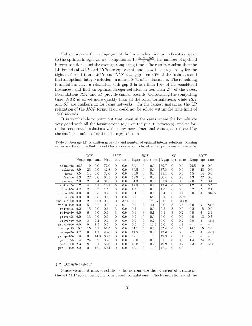
Table 3 reports the average gap of the linear relaxation bounds with respectto the optimal integer values, computed as 100 |LB−Opt||LB| , the number of optimalinteger solutions, and the average computing time. The results confirm that theLP bounds of MCF and GCS are equivalent, and show that they are by far thetightest formulations. MCF and GCS have gap 0 on 40% of the instances andfind an optimal integer solution on almost 30% of the instances. The remainingformulations have a relaxation with gap 0 in less than 10% of the consideredinstances, and find an optimal integer solution in less than 2% of the cases.Formulations RLT and SF provide similar bounds. Considering the computingtime, MTZ is solved more quickly than all the other formulations, while RLTand SF are challenging for large networks. On the largest instances, the LPrelaxation of the MCF formulation could not be solved within the time limit of1200 seconds.

It is worthwhile to point out that, even in the cases where the bounds arevery good with all the formulations (e.g., on the prc-f instances), weaker for-mulations provide solutions with many more fractional values, as reflected bythe smaller number of optimal integer solutions.

Table 3: Average LP relaxation gaps (%) and number of optimal integer solutions. Missingvalues are due to time limit. rome99 instances are not included, since optima are not available.

GCS MTZ RLT SF MCF%gap opt time %gap opt time %gap opt time %gap opt time %gap opt time

nobel-us 26.5 19 0.0 72.0 0 0.0 69.1 0 0.0 69.7 0 0.0 26.5 19 0.0atlanta 9.9 23 0.0 42.8 0 0.0 36.5 0 0.0 37.5 0 0.0 9.9 23 0.0

geant 5.5 14 0.0 32.0 0 0.0 30.9 0 0.0 31.1 0 0.0 5.5 14 0.0france 4.3 22 0.0 64.5 0 0.0 59.9 0 0.0 60.4 0 0.0 4.3 22 0.0

germany 2.0 2 0.4 31.5 0 0.0 31.3 0 0.0 31.3 0 0.0 2.0 2 0.4rnd-s-50 1.7 4 0.1 13.1 0 0.0 12.5 0 0.0 12.6 0 0.0 1.7 4 0.5

rnd-s-100 0.2 2 0.2 1.5 0 0.0 1.5 0 0.0 1.5 0 0.0 0.2 2 7.1rnd-s-200 0.0 0 0.5 0.4 0 0.0 0.4 0 0.5 0.4 0 0.4 0.0 0 345.5rnd-s-500 0.0 0 5.6 0.1 0 0.8 0.1 0 68.5 0.1 0 29.7 – – –

rnd-s-1000 0.0 2 51.9 0.0 0 37.4 0.0 0 792.5 0.0 0 319.8 – – –rnd-d-100 0.0 5 0.2 0.0 3 0.1 0.0 3 4.1 0.0 3 3.5 0.0 5 84.2rnd-d-25 0.2 15 0.0 0.6 3 0.0 0.5 4 0.0 0.5 3 0.0 0.2 15 0.0rnd-d-50 0.0 6 0.0 0.1 3 0.0 0.1 3 0.1 0.1 3 0.2 0.0 6 2.4prc-f-25 0.0 13 0.0 0.0 0 0.0 0.0 0 0.0 0.0 0 0.0 0.0 13 0.7prc-f-50 0.0 3 0.2 0.0 0 0.0 0.0 0 0.2 0.0 0 0.2 0.0 3 44.9

prc-f-100 0.0 0 2.5 0.0 0 0.0 0.0 0 11.0 0.0 0 4.1 – – –prc-p-25 10.1 15 0.1 91.5 0 0.0 87.1 0 0.0 87.4 0 0.0 10.1 15 2.6prc-p-50 8.2 6 1.1 80.6 0 0.0 77.5 0 0.2 77.6 0 0.2 8.2 6 89.3

prc-p-100 1.8 0 14.0 60.3 0 0.0 42.1 0 11.6 42.3 0 4.1 – – –prc-l-25 1.4 24 0.2 86.5 0 0.0 80.8 0 0.0 81.1 0 0.0 1.4 24 2.8prc-l-50 2.3 8 2.1 55.6 0 0.0 49.8 0 0.2 49.9 0 0.2 2.3 8 53.6

prc-l-100 2.2 0 12.1 60.4 0 0.0 42.1 0 11.0 42.4 0 4.0 – – –

4.2. Branch-and-cutSince we aim at integer solutions, let us compare the behavior of a state-of-

the-art MIP solver using the considered formulations. The formulations and the

13

separation procedures are implemented in C++ with IBM Ilog Cplex/Concert12.6, using default settings for the branch-and-cut.

For the polynomial-size extended formulations MTZ, RLT and SF, the fullmodel is built.

For GCS, we report results obtained with two different separation routines.In the approach denoted by GCS-StrongComp, the separation is carried out, onboth fractional and integer solutions, identifying the strongly connected compo-nents in the support graph induced by the variables xij . This can be done in aO(n+m) running time with Tarjan’s algorithm [35]. Once a strong componentS has been found, it is enough to check if Constraint (7) is violated for any of thenodes in S. This separation procedure is efficient, but not guaranteed to find allthe violated inequalities on fractional solutions. Correctness is preserved by thefact that the procedure is exact for integer solutions. In the approach denotedby GCS-MinCut, the separation is carried out on fractional solutions by solvinga sequence of Min Cut (or Max Flow) problems between each node and t. Solv-ing n−1 Min Cut problems yields an overall worst-case complexity of O(n3√m)using Goldberg-Tarjan’s highest-label preflow-push algorithm [20]. This way, allviolated inequalities are identified, although with a higher computational cost.Note that, on integer solutions, the faster strong component-based procedure issufficient, and, on fractional solutions, it is computationally convenient to trythe strong components procedure first, and resort to the Min-Cut separationonly if the heuristic finds no violated inequality. The same separation proce-dures are also used for MCF : when a violation is found for a node k, we addthe full set of Constraints (25)–(27) corresponding to that node.

To solve the Min Cut problems and identify the strongly connected compo-nents, we use the efficient implementations in the open-source LEMON GraphLibrary 1.3 [12]. We refer the interested reader to [13] for additional considera-tions on the separation of subtour elimination constraints for the ESPP.

A remark is in order. In a branch-and-cut algorithm, the generation of thecutting planes must be balanced with respect to the branching: adding toomany inequalities may hinder the solution of the LPs in the nodes, althoughbetter bounds result in fewer explored nodes. We use two parameters to controlthe trade-off between the quality of the lower bounds and the computing time tosolve the LPs. Specifically, given a solution x, we only consider the inequalitieswith a violation not smaller than ε (correctness is preserved on integer solutionsfor ε < 1), and we add at most ν of them (in particular, we select the firstν maximally violated). In Tables 4 and 5 we summarize a tuning procedurethat is carried out on a subset of 120 medium-size instances to identify the bestparameters for GCS-StrongComp and GCS-MinCut. We report the geometricmean of the time to optimality, the number of nodes and the number of addedcuts. The values are normalized, for each instance, with respect to the resultswith ε = 0.001 and ν = 1. The tables indicate that, in both cases, it isconvenient to add all the inequalities that are violated by the given toleranceε. According to these results, in the following experiments, we use ε = 0.8 andm = all for GCS-MinCut, and ε = 0.2,m = all for GCS-StrongComp.

Concerning the row generation for MCF, recall that for every violation we

14

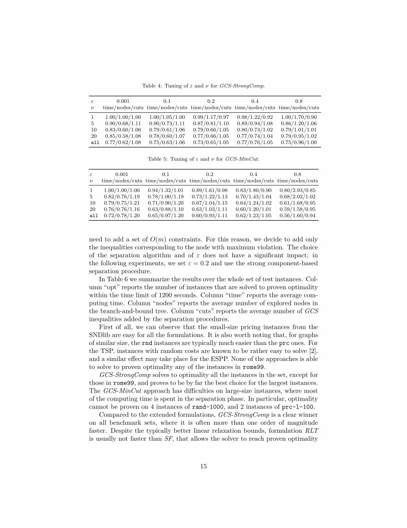
Table 4: Tuning of ε and ν for GCS-StrongComp.

ε 0.001 0.1 0.2 0.4 0.8ν time/nodes/cuts time/nodes/cuts time/nodes/cuts time/nodes/cuts time/nodes/cuts

1 1.00/1.00/1.00 1.00/1.05/1.00 0.99/1.17/0.97 0.98/1.22/0.92 1.00/1.70/0.905 0.90/0.68/1.11 0.90/0.73/1.11 0.87/0.81/1.10 0.89/0.94/1.08 0.86/1.20/1.0610 0.83/0.60/1.06 0.79/0.61/1.06 0.79/0.66/1.05 0.80/0.74/1.02 0.79/1.01/1.0120 0.85/0.58/1.08 0.78/0.60/1.07 0.77/0.66/1.05 0.77/0.74/1.04 0.79/0.95/1.02all 0.77/0.62/1.08 0.75/0.63/1.06 0.73/0.65/1.05 0.77/0.76/1.05 0.75/0.96/1.00

Table 5: Tuning of ε and ν for GCS-MinCut.

ε 0.001 0.1 0.2 0.4 0.8ν time/nodes/cuts time/nodes/cuts time/nodes/cuts time/nodes/cuts time/nodes/cuts

1 1.00/1.00/1.00 0.94/1.32/1.01 0.89/1.61/0.98 0.83/1.80/0.90 0.80/2.93/0.855 0.82/0.76/1.19 0.78/1.00/1.19 0.73/1.22/1.13 0.70/1.43/1.04 0.68/2.02/1.0210 0.79/0.75/1.21 0.71/0.90/1.20 0.67/1.04/1.15 0.64/1.24/1.02 0.61/1.68/0.9520 0.76/0.76/1.16 0.63/0.88/1.10 0.63/1.03/1.11 0.60/1.20/1.01 0.59/1.58/0.95all 0.72/0.78/1.20 0.65/0.97/1.20 0.60/0.93/1.11 0.62/1.23/1.05 0.56/1.60/0.94

need to add a set of O(m) constraints. For this reason, we decide to add onlythe inequalities corresponding to the node with maximum violation. The choiceof the separation algorithm and of ε does not have a significant impact; inthe following experiments, we set ε = 0.2 and use the strong component-basedseparation procedure.

In Table 6 we summarize the results over the whole set of test instances. Col-umn “opt” reports the number of instances that are solved to proven optimalitywithin the time limit of 1200 seconds. Column “time” reports the average com-puting time. Column “nodes” reports the average number of explored nodes inthe branch-and-bound tree. Column “cuts” reports the average number of GCSinequalities added by the separation procedures.

First of all, we can observe that the small-size pricing instances from theSNDlib are easy for all the formulations. It is also worth noting that, for graphsof similar size, the rnd instances are typically much easier than the prc ones. Forthe TSP, instances with random costs are known to be rather easy to solve [2],and a similar effect may take place for the ESPP. None of the approaches is ableto solve to proven optimality any of the instances in rome99.

GCS-StrongComp solves to optimality all the instances in the set, except forthose in rome99, and proves to be by far the best choice for the largest instances.The GCS-MinCut approach has difficulties on large-size instances, where mostof the computing time is spent in the separation phase. In particular, optimalitycannot be proven on 4 instances of rand-1000, and 2 instances of prc-l-100.

Compared to the extended formulations, GCS-StrongComp is a clear winneron all benchmark sets, where it is often more than one order of magnitudefaster. Despite the typically better linear relaxation bounds, formulation RLTis usually not faster than SF, that allows the solver to reach proven optimality

15

for a larger number of instances. Interestingly, while rather ineffective overall,formulation MTZ yields good results on the rnd instances. This might be dueto the fact that, on the rnd set, all the extended formulations have similarlygood linear relaxation bounds, and it probably pays off to have an LP of smallersize.

Formulation MCF, despite the tight linear relaxation, appears to be tooheavy to be of practical interest. On small-sized instances, very few B&B nodesare necessary. However, this is not enough to overcome the computational loadrequired by solving the linear relaxation: even with a row-generation approach,the size of the LP grows quickly. On graphs with 100 or more nodes, only asmall fraction of the instances can be solved within the time limit. On the largestgraphs, the instances in rnd-s-1000 and rome99, the solver quickly reaches thememory limit of 16 GB.

Figure 3 summarizes the computational experiments with a performanceprofile. On the y-axis, we report the fraction of all the instances that are solvedto optimality within the time on the x-axis (in logarithmic scale).

GCS-StrongComp is the topmost curve, solving more than 85% of the in-stances within 10 seconds. GCS-MinCut is not far behind, although it is gen-erally slower. Both solve around 95% of the instances within 1200 seconds.Formulations RLT, SF and MTZ yield similar results on the easiest instances,although, overall, only less than 70% of the instances are solved to optimalitywith MTZ, while SF and RLT reach, respectively, 90% and 87%. With theMCF approach (bottom curve), Cplex is already significantly slower on the eas-iest instances, and solves the smallest fraction of the instances (around 65%).

10�1 100 101 102 10310

20

30

40

50

60

70

80

90

100

GCS-StrongCompGCS-MinCutSFRLTMTZMCF

Figure 3: Fraction of instances solved to optimality within a given time (seconds). The x-axisis in logarithmic scale.

16

5. Conclusions

We have analyzed integer programming formulations for the ESPP, includingformulations not yet appeared in the literature.

The polyhedral results in Section 3 provide a partial hierarchy among theESPP formulations, and prove that the strong extended formulation MCF hasa projection on the space of the arc variables which is equivalent to the poly-tope of the GCS formulation, that has exponentially many subtour eliminationconstraints.

It is also important to understand how effective the formulations are from acomputational point of view. In this regard, we report a set of extensive com-putational experiments, suggesting that the extended formulations are inferiorfor all practical purposes, and the dynamic separation of subtour eliminationconstraints appears to be the best option when tackling the ESPP as an integerprogram. The GCS approach with the strong component-based separation pro-cedure is able to solve small-sized instances in a few seconds and medium-sizedinstances, with up to 1000 nodes, within a minute, but it is still not sufficient tosolve large-scale problems. When the implementation of a separation procedureis not possible or convenient, formulation SF is probably the best choice.

It seems likely that the development of good primal heuristics and additionalstrong valid inequalities, possibly extended from of the ATSP (e.g., 2-matchingor comb inequalities), might further speed up the computing times and allow thesolution of larger-sized instances. It might also be useful to borrow techniquesfrom the typical approaches used for the ESPPRC, such as a preprocessing phasewith the aim of reducing the search space.

Acknowledgments

The author would like to thank the two anonymous referees for the usefulcomments that helped improve the quality of the manuscript.

References

[1] Amaldi, E., Coniglio, S., Taccari, L., 2014. Maximum throughput networkrouting subject to fair flow allocation. In: ISCO. Vol. 8596 of Lecture Notesin Computer Science. Springer, pp. 1–12.

[2] Applegate, D. L., Bixby, R. E., Cook, W. J., Chvátal, V., 2006. The travel-ing salesman problem: a computational study. Princeton University Press.

[3] Balas, E., 1989. The prize collecting traveling salesman problem. Networks19 (6), 621–636.

[4] Balas, E., 2005. Projection, lifting and extended formulation in integer andcombinatorial optimization. Annals of Operations Research 140 (1), 125–161.

17

[5] Bauer, P., Linderoth, J. T., Savelsbergh, M. W., 2002. A branch and cutapproach to the cardinality constrained circuit problem. Mathematical Pro-gramming 91 (2), 307–348.

[6] Beasley, J., Christofides, N., 1989. An algorithm for the resource con-strained shortest path problem. Networks 19 (4), 379–394.

[7] Björklund, A., Husfeldt, T., Khanna, S., 2004. Approximating longestdirected paths and cycles. In: Automata, Languages and Programming.Springer, pp. 222–233.

[8] Boland, N., Dethridge, J., Dumitrescu, I., 2006. Accelerated label settingalgorithms for the elementary resource constrained shortest path problem.Operations Research Letters 34 (1), 58–68.

[9] Claus, A., 1984. A new formulation for the travelling salesman problem.SIAM Journal on Algebraic Discrete Methods 5 (1), 21–25.

[10] Dantzig, G., Fulkerson, R., Johnson, S., 1954. Solution of a large-scaletraveling-salesman problem. Operations Research 2 (4), 393–410.

[11] Demetrescu, C., Goldberg, A. V., Johnson, D. S., 2009. The Shortest PathProblem: Ninth DIMACS Implementation Challenge. Vol. 74. AMS.

[12] Dezső, B., Jüttner, A., Kovács, P., 2011. LEMON – an open source C++graph template library. Electronic Notes in Theoretical Computer Science264 (5), 23–45.

[13] Drexl, M., 2013. A note on the separation of subtour elimination constraintsin elementary shortest path problems. European Journal of OperationalResearch 229 (3), 595–598.

[14] Drexl, M., Irnich, S., 2014. Solving elementary shortest-path problems asmixed-integer programs. OR Spectrum 36 (2), 281–296.

[15] Feillet, D., Dejax, P., Gendreau, M., Gueguen, C., 2004. An exact algo-rithm for the elementary shortest path problem with resource constraints:Application to some vehicle routing problems. Networks 44 (3), 216–229.

[16] Fischetti, M., Gonzalez, J. J. S., Toth, P., 1998. Solving the orienteeringproblem through branch-and-cut. INFORMS Journal on Computing 10 (2),133–148.

[17] Gabow, H. N., 2007. Finding paths and cycles of superpolylogarithmiclength. SIAM Journal on Computing 36 (6), 1648–1671.

[18] Gavish, B., Graves, S. C., 1978. The travelling salesman problem andrelated problems. Working Paper GR-078-78, Massachusetts Institute ofTechnology.

18

[19] Gendreau, M., Laporte, G., 1998. A branch-and-cut algorithm for the undi-rected selective traveling salesman problem. Networks 32, 263–273.

[20] Goldberg, A. V., Tarjan, R. E., 1988. A new approach to the maximum-flowproblem. Journal of the ACM (JACM) 35 (4), 921–940.

[21] Haouari, M., Maculan, N., Mrad, M., 2013. Enhanced compact modelsfor the connected subgraph problem and for the shortest path problem indigraphs with negative cycles. Computers & Operations Research 40 (10),2485–2492.

[22] Ibrahim, M., Maculan, N., Minoux, M., 2009. A strong flow-based for-mulation for the shortest path problem in digraphs with negative cycles.International Transactions in Operational Research 16 (3), 361–369.

[23] Irnich, S., Desaulniers, G., 2005. Shortest Path Problems with ResourceConstraints. Springer, Ch. 2, pp. 33–65.

[24] Jepsen, M., Petersen, B., Spoorendonk, S., Pisinger, D., 2008. Subset-row inequalities applied to the vehicle-routing problem with time windows.Operations Research 56 (2), 497–511.

[25] Jepsen, M. K., Petersen, B., Spoorendonk, S., 2008. A branch-and-cut algo-rithm for the elementary shortest path problem with a capacity constraint.Tech. Rep. 08/01, Department of Computer Science, University of Copen-hagen.

[26] Jepsen, M. K., Petersen, B., Spoorendonk, S., Pisinger, D., 2014. A branch-and-cut algorithm for the capacitated profitable tour problem. DiscreteOptimization 14, 78–96.

[27] Karger, D., Motwani, R., Ramkumar, G., 1997. On approximating thelongest path in a graph. Algorithmica 18 (1), 82–98.

[28] Miller, C. E., Tucker, A. W., Zemlin, R. A., 1960. Integer programmingformulation of traveling salesman problems. Journal of the ACM (JACM)7 (4), 326–329.

[29] Naddef, D., Rinaldi, G., 2002. Branch-and-cut algorithms for the capaci-tated VRP. SIAM Monographs on Discrete Mathematics and ApplicationsPhiladelphia, PA, Ch. 3, pp. 53–84.

[30] Orlowski, S., Wessäly, R., Pióro, M., Tomaszewski, A., 2010. SNDlib 1.0 -survivable network design library. Networks 55 (3), 276–286.

[31] Padberg, M., Sung, T.-Y., 1991. An analytical comparison of different for-mulations of the travelling salesman problem. Mathematical Programming52 (1-3), 315–357.

19

[32] Righini, G., Salani, M., 2006. Symmetry helps: bounded bi-directional dy-namic programming for the elementary shortest path problem with resourceconstraints. Discrete Optimization 3 (3), 255–273.

[33] Sherali, H. D., Adams, W. P., 1990. A hierarchy of relaxations betweenthe continuous and convex hull representations for zero-one programmingproblems. SIAM Journal on Discrete Mathematics 3 (3), 411–430.

[34] Taccari, L., 2015. Mixed-integer programming models and methods forbilevel fair network optimization and energy cogeneration planning. Ph.D.thesis, Politecnico di Milano, Milano.

[35] Tarjan, R., 1972. Depth-first search and linear graph algorithms. SIAMJournal on Computing 1 (2), 146–160.

[36] Vansteenwegen, P., Souffriau, W., Oudheusden, D. V., 2011. The orienteer-ing problem: A survey. European Journal of Operational Research 209 (1),1–10.

[37] Wong, R., 1980. Integer programming formulations of the travelling sales-man problem. In: Proceedings of the IEEE international conference oncircuits and computers. pp. 149–152.

20

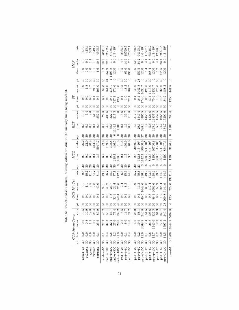
Table6:

Branch-an

d-cutresults.

Missing

values

aredu

eto

themem

orylim

itbe

ingreached.

GC

S-St

rong

Com

pG

CS-

Min

Cut

MT

ZR

LTSF

MC

Fop

tti

me

node

scu

tsop

tti

me

node

scu

tsop

tti

me

node

sop

tti

me

node

sop

tti

me

node

sop

tti

me

node

scu

ts

nobe

l-us

300.0

0.6

10.5

300.0

3.1

9.6

300.0

26.2

300.0

19.1

300.0

9.0

300.0

1.0

397.3

atla

nta

300.0

0.8

10.9

300.0

1.1

10.7

300.0

22.0

300.0

7.4

300.0

1.8

300.0

0.6

415.4

gean

t30

0.0

1.1

12.8

300.0

2.5

11.5

290.0

20.9

300.0

9.6

300.0

4.7

300.0

1.1

633.7

fran

ce30

0.0

0.7

26.4

300.0

2.8

24.7

300.1

344.3

300.1

51.1

300.1

21.1

300.1

1.0

1549.7

germ

any

300.1

25.6

89.9

300.1

40.0

81.4

303.5

5947.7

300.4

352.5

300.7

403.0

301.6

10.6

4595.3

rnd-

s-50

300.1

22.3

46.2

300.1

33.1

43.4

300.2

82.9

300.2

79.8

300.2

59.0

303.2

18.3

6611.3

rnd-

s-10

030

0.4

37.3

56.1

300.5

40.2

56.7

300.9

189.5

304.3

403.6

302.0

151.0

24557.9

72.3

32582.7

rnd-

s-20

030

0.8

22.1

66.7

301.8

25.7

75.0

309.0

308.8

3038.5

322.1

3019.7

218.1

11193.8

1.9

87376.9

rnd-

s-50

030

4.2

27.6

77.4

3032

.329.4

77.1

30218.1

496.5

61104.1

217.3

26557.1

373.6

01200

0.0

2.5

·105

rnd-

s-10

0030

21.3

29.6

139.2

2635

2.4

25.6

142.4

31158.3

51.8

01200

0.0

01200

0.0

0–

––

rnd-

d-25

300.0

2.2

6.5

300.0

2.4

6.6

300.1

31.6

300.1

13.6

300.1

10.5

300.5

4.6

2365.5

rnd-

d-50

300.1

8.0

14.7

300.1

8.3

15.3

301.7

460.9

301.3

39.7

301.0

18.2

3069.0

14.6

18769.7

rnd-

d-10

030

0.4

14.0

24.2

300.8

16.1

24.8

303.5

70.0

3030.0

113.8

3022.1

107.7

6996.0

2.5

67352.1

prc-

f-25

300.0

4.0

25.0

300.0

3.9

25.7

302.8

3059.3

301.0

317.1

300.4

49.6

303.6

13.9

7978.8

prc-

f-50

300.2

19.9

68.1

300.3

16.3

70.8

23332.8

1.3

·105

3029.9

1346.4

3016.4

1047.8

28459.5

34.2

64155.9

prc-

f-10

030

11.0

2068

.924

6.8

3040

.516

49.6

236.6

31142.7

30600.6

27328.0

3465.5

30174.61633.7

01200

0.0

4.6

·105

prc-

p-25

300.1

7.4

54.5

300.2

30.8

49.2

16688.2

8.1

·105

301.4

1455.7

300.9

426.6

305.4

4.1

11687.6

prc-

p-50

300.6

26.8

103.6

300.8

112.4

103.3

11872.3

4.5

·105

305.5

1224.6

3013.4

1113.0

30288.4

11.8

65648.2

prc-

p-10

030

12.7

1243

.032

5.3

3088

.130

03.6

428.2

01200

90700.8

29165.219837.3

3075.6

3432.7

01200

0.0

4.3

·105

prc-

l-25

300.2

12.3

64.3

300.2

50.9

59.5

10808.5

1.4

·106

305.3

1552.5

301.3

175.6

305.2

4.1

12078.0

prc-

l-50

300.9

77.3

169.7

301.2

188.4

164.0

51027.5

5.1

·105

3024.2

1068.5

3014.8

764.6

30248.5

23.4

59021.8

prc-

l-10

030

14.5

1597

.234

0.4

2820

9.861

44.9

444.6

01200

88407.3

30134.715209.0

3084.2

4188.2

01200

0.0

4.3

·105

rome

99012

0016

944.95668

.80

1200

728.013271.4

01200

3126.2

01200

780.4

01200

447.8

0–

––

21