InTech-Three Dimensional Stress Strain State of a Pipe

5

Three-Dimensional Stress-Strain State of a Pipe with Corrosion Damage

Under Complex Loading

S. Sherbakov Department of Theoretical and Applied Mechanics, Belarusian State University

Belarus

1. Introduction

In studies of the stress-stain state of models of pipeline sections without corrosion defects of a pipe, in the two-dimensional statement (cross section), pipes are usually modeled by a ring, whereas in the three-dimensional statement – by a thick-wall cylindrical shell [Ponomarev et al., 1958; Seleznev et al. 2005]. Usually, internal pressure or temperature is considered as a load applied to the pipe. The solution of the problems stated in this manner yields not bad results when a relatively not complicated procedure of calculation, both analytical and numerical, is adopted. The presence of corrosion damage at the inner surface of the pipe (Figures 1, 2), being a particular three-dimensional concentrator of stresses, requires a special approach to defening the stress-strain state. In addition, account should be taken of a simultaneous compound action of such loading factors as internal pressure and friction of the mineral oil flow over the inner surface of the pipe, as well as of soil. The analysis of the known references to articles shows that the problem of investigating the spatial stress-strain states of the pipe with regard to its corrosion damage with the account of various types of loading has not been stated up to now. In essence, the problems of

determining individual stress-strain states under the action of internal pressure ( ( )pijσ , ( )p

ijε )

or temperature ( ( )Tijσ , ( )T

ijε ) [Ainbinder et al., 1982; Borodavkin et al., 1984; Grachev et al.,

1982; Dertsakyan et al., 1977; Mirkin et al., 1991; O'Grady et al., 1992] are under consideration. The problem of determining stress-strain state caused by wall friction due to

viscous fluid motion ( ( )ijτσ , ( )

ijτε ), as well as the most general problems of determining

( )pij

τσ + , ( )pij

τε + ; ( )p Tijσ + , ( )p T

ijε + ; ( )p Tij

τσ + + ( )p Tij

τε + + has not been stated. In addition, the

problems of stress-strain state determination are usually being solved for shell models of a

pipe. Although, for example, in [Seleznev et al. 2005] ( )pijσ is described for the three-

dimensional model of the section of the pipe with corrosion damage. Therefore the statement and solutions of the problem of determining three-dimensional stress-strain state of the models of pipes with corrosion defects under the action of internal pressure, friction caused by oil flow and temperature discussed in the present chapter are

www.intechopen.com

Tribology - Lubricants and Lubrication

140

important for pipeline systems and such related disciplines as solid mechanics, fluid mechanics and tribology.

2. Statement of the problem

The present Chapter deals with some of the results of investigation of the three-dimensional stress-strain state of the model of a pipe with corrosion damage (Figure 2).

Fig. 1. Simplified scheme of elliptical corrosion damage at the inner surface of the pipe displaying reduced wall thickness inside the damage

In calculations, the following basic loads applied to the pipe were taken into consideration:

• internal pressure

1

,r r rpσ = = (1)

where r1 is the inner radius of the pipe;

• mineral oil friction over the inner surface of the pipe, thus exciting wall tangential stresses

1

0 ,rz r rτ τ= = (2)

τ0 – tangential forces modeling the viscous fluid friction force over the inner surface of the pipe;

• change of the thermodynamic state (temperature) of the pipe

1 2

,r rT T T− = Δ (3)

where r2 is the outer radius of the pipe. It should be emphasized that in the presence of corrosion damage

( )1 1 , ,r r zϕ= (4)

where ϕ and z are the components of the cylindrical coordinate system (r, ϕ, z).

www.intechopen.com

Three-Dimensional Stress-Strain State of a Pipe with Corrosion Damage Under Complex Loading

141

Fig. 2. Solid model of the neighborhood of the pipe with corrosion damage

The distinctive feature of computer finite-element modeling of pipes of trunk pipelines with corrosion damage lies in the opportunity to assign different boundary conditions for the outer surface of the pipe. So, for loads (1)–(3), consideration is made of different restrictions on displacements of the outer surface of the pipe: a. no pipeline fixing

2

0,r r rσ = = (5)

b. no displacements of the outer surface of the pipe in the x and y directions and in the z direction on the right end

2 2

0, 0,x y zr r z Lr ru u u= === = = (6)

c. no displacements of the outer surface of the pipe in all directions

2 22

0,x y zr r r rr ru u u= === = = (7)

d. contact between the pipe and soil where no displacements of the soil outer surface take place

2 2

2 2 2

3 3

(1) (2)

(1) (2) (1)

,

,

0

r rr r r r

nr r r r r r

x yr r r r

f

u u

τ τ

σ σσ σ σ

= =

= = == =

= −= − =

= = (8)

where the superscript 1 means the pipe, whereas 2 – soil, στ is the tangential component of the stress vector, f is the friction coefficient, and r3 is the soil outer radius.

www.intechopen.com


142

With the use of the pipeline fixing (type a), tests of the pipe dug out of soil (in the air) are

modeled. The stress-strain state of a pipe lying in hard soil without friction in the axial

direction is modeled by means of pipe fixing (type b) while that of a pipe lying in hard soil

and rigidly connected with it – by means of pipe fixing (type c). Subject to boundary

conditions (8) (type d), a pipe lying in soil having particular mechanical characteristics is

modeled.

Thus, the problem has been stated to make a comparative analysis of the stress-strain states

of the pipe with corrosion damage for different combinations of boundary conditions (1)–

(3), (6)–(8):

( ) ( ) ( ) ( ) ( ) ( )

( ) ( ) ( ) ( ) ( ) ( )

, ; , ; , ;

, ; , ; , .

p p T Tij ij ij ij ij ij

p p p T p T p T p Tij ij ij ij ij ij

τ ττ τ τ τ

σ ε σ ε σ εσ ε σ ε σ ε+ + + + + + + + (9)

where the superscripts p, τ, and T correspond to the stress states caused by internal

pressure, friction force over the inner surface of the pipe, and temperature.

In the case of the elastic relationship between stresses and strains, the stress states in (9) are

connected by the following relations

( ) ( ) ( )

( ) ( ) ( )

( ) ( ) ( ) ( )

,

,

.

p pij ij ij

p T p Tij ij ij

p T p Tij ij ij ij

τ τ

τ τ

σ σ σσ σ σσ σ σ σ

+++ +

= += += + +

(10)

Further, some of the solutions to more than 70 problems of studying the stress-strain state of

the pipe cross section in the damage area (dot-and-dash line in Figure 1) [Kostyuchenko et

al., 2007a; 2007b; Sherbakov et al., 2007b; 2008a; 2008b; Sherbakov, 2007b; Sosnovskiy et al.,

2008] are analyzed. These two-dimensional problems mainly describe the stress-strain states

of straight pipes with different-profile damage along the axis. Also, with the use of the

finite-element method implemented in the software ANSYS, the essentially three-

dimensional stress-strain state of the pipe in the three-dimensional damage area (Figure 1)

was investigated.

3. Wall friction in the turbulent mineral oil flow in the pipe with corrosion damage

Within the framework of the present work, hydrodynamic calculation was made of the

motion characteristics of a viscous, incompressible, steady, isothermal fluid in a cylindrical

channel that models a pipe and in a cylindrical channel with geometric characteristics with

regard to the peculiarities of a pipe with corrosion damage (see, Sect. 2). Calculations were

performed for the initial incoming flow velocities υ0: 1 m/sec and 10 m/sec.

The kinematic viscosity of fluid was taken equal to vK = 1.4 10-4 m2/sec, the viscous fluid

density – 865 kg/m3. The calculated Reynolds numbers will be, respectively,

01m/sec 4 2

1m /sec*0.612mRe 4371.43,

1.4*10 m /secK

Dυν −= = = (11)

www.intechopen.com


143

010 m/sec 4 2

10m /sec*0.612mRe 43714.3.

1.4*10 m /secK

Dυν −= = = (12)

The critical Reynolds number (a transition from a laminar to a turbulent flow) for a viscous

fluid moving in a round pipe is Recr ≈ 2300. Thus, the turbulent flow motion should be

considered in our problem. The software Fluent calculations used the turbulence k – ε model for modeling turbulent flow viscosity [Launder et al., 1972; Rodi, 1976]. As boundary conditions the following parameters were used: at the incoming flow surface the initial turbulence level equal to 7% was assigned; at the pipe walls the fixing conditions and the logarithmic velocity profile were predetermined; in the pipe the fluid pressure equal to 4 МPа was set. Calculations of the steady regime of the fluid flow (quasi-parabolic turbulent velocity profile of the incoming flow) and of the unsteady regime (rectangular velocity profile of the incoming flow) were made. In the problems with a rectangular velocity profile of the incoming flow

10,x rx

υ υ= = (13)

The unsteady regime of the fluid flow was considered. In the problems with a quasi-parabolic turbulent velocity profile, at the entrance surface of the pipe the empirically found profile of the initial velocity was assigned, which is determined by the formula: - for the two-dimensional case

1

70

max max 0 100

21 , 1.1428 ,0 2 ,

2x x

r rr r

rυ υ υ υ=

⎛ ⎞−= − = ≤ ≤⎜ ⎟⎝ ⎠ (14)

- for the three-dimensional case

1

72 2

max max 0 100

1 , 1.2244 , ,0 .x x

rr y z r r

rυ υ υ υ=

⎛ ⎞= − = = + ≤ ≤⎜ ⎟⎝ ⎠ (15)

The calculation results have shown that the motion becomes steady (as the flow moves in the pipe, the quasi-parabolic turbulent profile of the longitudinal velocity Vx develops) at some distance from the entrance (left) surface of the pipe (Figure 3). So, from Figure 4 it is seen that for the quasi-parabolic velocity profile of the incoming flow the zone of the steady motion begins earlier than for the rectangular profile. Further, we will consider the results obtained for the velocity profiles of the incoming flow calculated in accordance to (14) and (15). Consider the flow turbulence intensity being the ratio of the root-mean-square fluctuation

velocity u′ to the average flow velocity uavg (Figure 5).

'

,avg

uI

u= (16)

At the surface of the incoming flow, the turbulence intensity is calculated by the formula

www.intechopen.com


144

( ) 1080.16 Re , Re ,

H H

HD D

DI

υν

−= = (17)

where DH is the hydraulic diameter (for the round cross section: DH = 2r1 = 0.612 m), υ0 is the

incoming flow velocity, and v is the kinematic viscosity of oil (v = 1.4⋅10–4 m2/sec).

Fig. 3. Longitudinal velocity Vx (two-dimensional flow) for the quasi-parabolic turbulent

velocity profile of the incoming flow at υ0 = 1 m/sec

Fig. 4. Profiles of the longitudinal velocity Vx. over the pipe cross sections (three-dimensional

flow) for the quasi-parabolic turbulent velocity profile of the incoming flow at υ0 = 1 m/sec

www.intechopen.com


145

Fig. 5. Turbulence intensity (two-dimensional pipe flow, quasi-parabolic turbulent velocity

profile, υ0 = 1 m/sec)

Fig. 6. Transverse velocity Vy for the two-dimensional flow in the pipe with corrosion

damage at υ0 = 10 m/sec

The zone of the unsteady turbulent motion is characterized by the higher turbulence

intensity (vortex formation) in comparison with the remaining region of the pipe (Figure 5).

The highest intensity is observed in the steady motion zone, which is especially noticeable in

the calculations with the initial velocity of 1 m/sec in the pipe wall region, whereas the

lowest one – at the flow symmetry axis.

At high initial flow velocity values the vortex formation rate is higher.

www.intechopen.com


146

It should be emphasized that at a higher value of the initial flow velocity, the instability

region is longer: at υ0 = 1 m/sec its length is about 2 m, while at υ0 = 10 m /sec its length is

about 5 m.

The behavior of the motion (steady or unsteady) exerts an influence on the value of wall

stresses. In the unsteady motion zone, they are essentially higher as against the appropriate

stresses in the identical steady motion zone.

These figures illustrate that at that place of the pipe, where the fluid motion becomes steady,

the value of tangential stress at υ0 = 1 m/sec is approximately equal to 8 Pa, whereas at υ0 =

10 m/sec it is about 240 Pa.

The results as presented above are peculiar for a pipe with corrosion damage and without it.

At the same time, the presence of corrosion damage affects the kinematics of the moving

flow in calculations with both the rectangular profile of the initial flow velocity and the

quasi-parabolic turbulent one. In this domain of geometry, there appear transverse

displacements that form a recirculation zone (Figure 7).

Fig. 7. Transverse velocity Vz for the three-dimensional flow in the pipe with corrosion

damage at υ0 = 10 m/sec

The corrosion spot exerts a profound effect on changes in wall tangential stresses in the area

of the pipe corrosion damage.

Figures 8 and 9 demonstrate that in the corrosion damage area, the values of wall tangential

stresses undergo jumping.

For the laminar fluid motion, the value of tangential stresses at the pipe wall is calculated by

the following formula [Sedov, 2004]:

00

0

4,

yx d

y x dr r

υυ μυυτ μ μ∂⎛ ⎞∂= + = =⎜ ⎟⎜ ⎟∂ ∂⎝ ⎠ (18)

where μ = υ⋅ρ = 1.4⋅10–4⋅865 = 0.1211 kg/(m*sec) is the molecular viscosity, r0 = 0.306 m is the pipe radius.

www.intechopen.com


147

Fig. 8. Wall tangential stresses at the pipe wall: stresses at y = f(x), stresses at y = 2r1 for the

two-dimensional flow in the pipe with corrosion damage at υ0 = 1 m/sec

Fig. 9. Wall tangential stresses at the pipe wall: stresses at y = f(x), stresses at y = 2r1 for the

two-dimensional flow in the pipe with corrosion damage at υ0 = 10 m/sec

Then τ0 for the velocities υ0 = 10 m/sec and υ0= 1 m/sec will be

10 10 0

4 0.1211 10 4 0.1211 115.83 Pa, 1.58 Pa.

0.306 0.306τ τ⋅ ⋅ ⋅ ⋅= = = = (19)

The expression for the tangential stresses with regard to the turbulence is of the form [Sedov, 2004]:

0 ' ' ' ( ) .y yx x

xy xy x y ty x y x

υ υυ υτ τ τ μ ρυ υ μ μ∂ ∂⎛ ⎞ ⎛ ⎞∂ ∂= + = + − = + +⎜ ⎟ ⎜ ⎟⎜ ⎟ ⎜ ⎟∂ ∂ ∂ ∂⎝ ⎠ ⎝ ⎠ (20)

The last formula and the analysis of the calculations enable evaluating the turbulence influence on the value of tangential stresses at the pipe wall. As indicated above, at different

profiles and initial velocity values the tangential stresses were obtained: at υ0 = 1 m/sec:

www.intechopen.com


148

τxy = τw ≈ 8 Pa, at υ0 = 10 m/sec: τxy = τw ≈ 240 Pa. The value of the turbulent stress (Reynolds stress):

at υ0 = 1 m/sec :

0' ' ' 8 1.58 6.42Pa,

yxxy x y t xy

y x

υυτ ρυ υ μ τ τ∂⎛ ⎞∂= − = + = − = − =⎜ ⎟⎜ ⎟∂ ∂⎝ ⎠ (21)

at υ0= 10 m/sec :

0' ' '

240 15.83 224.17 Pa,

yxxy x y t xy

y x

υυτ ρυ υ μ τ τ∂⎛ ⎞∂= − = + = − =⎜ ⎟⎜ ⎟∂ ∂⎝ ⎠= − =

(22)

The results obtained are evident of the fact that the turbulence much contributes to the formation of wall tangential stresses. At the higher turbulence intensity (it is especially high in the pipe wall region), Reynolds stresses increase, too. I.e., the turbulence stresses are:

at υ0 = 1 m/sec : 0 8 1.58100% 100% 80.25%;

8

xy

xy

τ ττ− −= = (23)

at υ0 = 10 m/sec : 0 240 15.83100% 100% 93.4%.

240

xy

xy

τ ττ− −= = (24)

The analysis as made above shows that the calculation of the motion of a viscous fluid in the pipe as laminar can result in a highly distorted distribution pattern of the tangential stresses at the inner surface of the pipe. It can be concluded that the analysis of viscous fluid friction, when the flow interacts with the pipe wall, must be performed on the basis of the calculation of flow motion as essentially turbulent one.

4. Analytical solutions for the stress-strain state of the pipeline model under the action of internal pressure and temperature difference

In the simplified analytical statement, the problem of calculating the stress-strain state of a long cylindrical pipe reduces to the problem of the strain of a thin ring loaded with a pressure p1 uniformly distributed over its inner wall and also with a pressure p2 uniformly distributed over the outer surface of the ring (Figure 10). Operating conditions of the ring do not vary depending on whether it is considered either as isolated or as a part of the long cylinder. Work [Ponomarev et al., 1958] and many other publications contain the classical solution to this problem based on solving the following differential equation for radial displacements:

2

2 2

1 10.r r

r

d u duu

r drdr r+ − = (25)

The general solution of this equation is of the form:

1 2

1.ru C r C

r= + (26)

www.intechopen.com


149

With the use of the relationship between stresses and strains, and also of Hook’s law, it is

possible to determine integration constants С1and С2 under the boundary conditions of the

form:

1

2

1

2

,

.

r r r

r r r

p

p

σσ

==

=−=− (27)

where р1 is the internal pressure; р2 is the external pressure.

Fig. 10. Loading diagram of the circular cavity of the pipe

In such a case, the general formulas for stresses at any pipe point have the following form:

2 2 2 21 1 2 2 1 2 1 2

2 2 2 2 22 1 2 1

2 2 2 21 1 2 2 1 2 1 2

2 2 2 2 22 1 2 1

( ) 1,

( ) 1.

r

p r p r p p r r

r r r r r

p r p r p p r r

r r r r rϕ

σσ

− −= −− −− −= +− −

(28)

Assuming that the cylinder is loaded only with the internal pressure (р1 = p, р2 = 0), the

following expressions are obtained for the stresses based on the internal pressure:

( ) ( )2 2

12 122 2 2 22 12 2 12

1 11 , 1 ,

1 1

ppr r r

r r r r

k k

p pk k k k

ϕσσ ⎛ ⎞ ⎛ ⎞= − = +⎜ ⎟ ⎜ ⎟⎜ ⎟ ⎜ ⎟− −⎝ ⎠ ⎝ ⎠ (29)

where kr2 = r /r2, kr12 = r1 / r2

To analyze the rigid fixing of the outer surface of the pipeline, as one of the equations of the

boundary conditions we choose expression (26) for displacements, the value of which tends

to zero at the outer surface of the model. As the secondary boundary condition we use an

expression for stresses at the inner surface of the cylinder from (27):

1 2

1 , 0.r rr r r rp uσ = ==− = (30)

Then, the expressions for the stresses will assume the form:

www.intechopen.com


150

( )

( )

2 212 2 1 12 22 12 1 1

2 212 2 1 12 22 12 1 1

(1 ) ( 1),

(1 ) ( 1)

(1 ) ( 1).

(1 ) ( 1)

pr r r

r r

p

r r

r r

k k

p k k

k k

p k k

ϕ

σ ν νν ν

σ ν νν ν

+ − −= − + − −+ + −= − + − −

(31)

Consider a long thick-wall pipe, whose wall temperature t varies across the wall, but is

constant along the pipe, i. e., t = t(r) [Ponomarev et al., 1958].

If the heat flux is steady and if the temperature of the outer surface of the pipe is equal to

zero and that of the inner surface is designated as Т, then from the theory of heat transfer it

follows that the dependence of the temperature t on the radius r is given by the formula

212

ln ,ln

rr

Tt k

k= (32)

Any other boundary conditions can be obtained by making uniform heating or cooling,

which does not cause any stresses. Thus, the quantity Т in essence represents the

temperature difference ΔT of the inner and outer surfaces of the pipe.

As the temperature is constant along the pipe, it can be considered that cross sections at a

sufficient distance from the pipe ends remain plane, and the strain εz is a constant quantity.

The temperature influence can be taken into account if the strains due to stresses are added

with the uniform temperature expansion Δε = αΔT where α is the linear expansion

coefficient of material.

The stress-strain state in the presence of the temperature difference between the pipe walls

can be determined by solving the differential equation [Ponomarev et al., 1958]:

2

12 2

1

1 1.

1

d u du u dt

r dr drdr r

ν αν++ − = − (33)

Subject to the boundary conditions

1 2

0, 0.r rr r r rσ σ= == = (34)

Having solved boundary-value problem (33), (34), the expressions for stresses are of the

form:

( ) ( )( ) ( )( ) ( )

2121

2 122 212 12 2

2121

2 122 212 12 2

2121

2 12212 12

1 1ln 1 ln ,

2 1 ln 1

1 11 ln 1 ln ,

2 1 ln 1

211 2 ln ln ,

2 1 ln 1

T rr r r

r r r

T rr r

r r r

T rz r r

r r

kE Tk k

k k k

kE Tk k

k k k

kE Tk k

k k

ϕ

ασ νασ νασ ν

⎡ ⎤⎛ ⎞Δ= − − −⎢ ⎥⎜ ⎟⎜ ⎟− −⎢ ⎥⎝ ⎠⎣ ⎦⎡ ⎤⎛ ⎞Δ= − − − +⎢ ⎥⎜ ⎟⎜ ⎟− −⎢ ⎥⎝ ⎠⎣ ⎦⎡ ⎤Δ= − − −⎢ ⎥− −⎢ ⎥⎣ ⎦

(35)

Figures 11–14 show the distribution of dimensionless stresses (29), (31), (35) along r and their sums

www.intechopen.com


151

( ) ( ) ( ) , , , ,p T p T

i i i i r zσ σ σ ϕ+ = + = (36)

for kr12 = 0.8, v = 0.3, E1αT / p = 10 (for example, at E1 = 2⋅1011 Pa, α = 10-5°С-1, ΔT = 20 °C). These figures well illustrate the essential influence of the temperature and the procedure of

fixing the pipe on its stress-strain state.

Fig. 11. Radial stresses for problems (25), (27) and (33), (34) at r1 ≤ r ≤ r2

Compare the distribution of the stresses calculated analytically with the use of (31) for a

non-damaged pipe with the finite-element calculation results by plotting the graphs of the

pipe thickness stress distribution (Figures 1.15–1.16). To make calculation, take the following

initial data: inner and outer radii r1= 0.306 m and r2= 0.315 m, p1= 4М Pa, p2= 0, Е = 2⋅1011 Pa,

ν = 0.3.

Fig. 12. Circumferential stresses for problems (25), (27) and (33), (34) at r1 ≤ r ≤ r2

www.intechopen.com


152

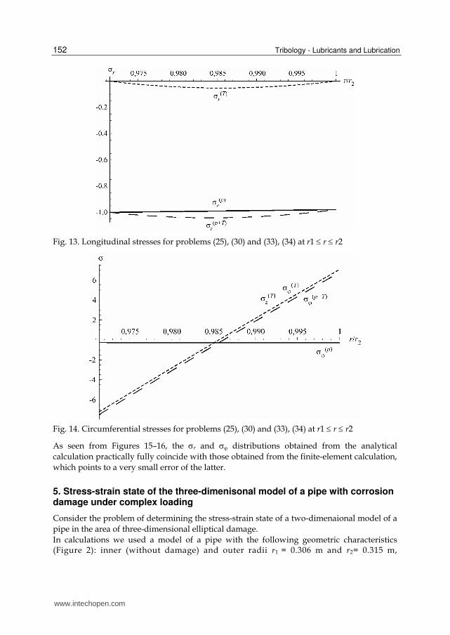
Fig. 13. Longitudinal stresses for problems (25), (30) and (33), (34) at r1 ≤ r ≤ r2

Fig. 14. Circumferential stresses for problems (25), (30) and (33), (34) at r1 ≤ r ≤ r2

As seen from Figures 15–16, the σr and σϕ distributions obtained from the analytical

calculation practically fully coincide with those obtained from the finite-element calculation,

which points to a very small error of the latter.

5. Stress-strain state of the three-dimenisonal model of a pipe with corrosion damage under complex loading

Consider the problem of determining the stress-strain state of a two-dimenaional model of a

pipe in the area of three-dimensional elliptical damage.

In calculations we used a model of a pipe with the following geometric characteristics (Figure 2): inner (without damage) and outer radii r1 = 0.306 m and r2= 0.315 m,

www.intechopen.com


153

Fig. 15. Radial stress distribution for the analytical calculation ( ( )prσ ), for the two-

dimensional computer model ( ( )2Drσ ), for the three-dimensional computer model ( ( )3D

rσ )

Fig. 16. Circumferential stress distribution for the analytical calculation ( ( )pϕσ ), for the two-

dimensional computer model ( ( )2Dϕσ ), for the three-dimensional computer model ( ( )3Dϕσ )

respectively, the length of the calculated pipe section L=3 m, sizes of elliptical corrosion damage length × width × depth – 0.8 m × 0.4 m × 0.0034 m.

The pipe mateial had the following characteristics: elasticity modulus E1 = 2⋅1011 Pa, Poisson’s coefficient v1 = 0.3, temperature expansion coefficient α = 10-5 °С-1, thermal conductivity k = 43 W/(m°С), and the soil parameters were: E2 = 1.5⋅109 Pa, Poisson’s coefficient v2 = 0.5. The coefficient of friction between the pipe and soil was μ = 0.5. The internal pressure in the pipe (1) is:

1

4 MPa.r r rpσ = = = (37)

www.intechopen.com


154

The temperature diffference between the pipe walls is (3)

1 2

20 .оr rT T T С− = Δ = (38)

The value of internal tangential stresses (wall friction) (2) is determined from the hydrodynamic calculation of the turbulent motion of a viscous fluid in the pipe. Calculations in the absence of fixing of the outer surface of the pipe and in the presence of the friction force over the inner surface (2) were made for 1/2 of the main model (Figure 2), since in this case (in the presence of friction) the calculation model has only one symmetry plane. In the absence of outer surface fixing, calculations were made for 1/4 of the model of the pipeline section since the boundary conditions of form (2) are also absent and, hence, the model has two symmetry planes. The investigation of the stress state of the pipe in soil is peformed for 1/4 of the main model of the pipe placed inside a hollow elastic cylinder modeling soil (Figure 17). In calculations without temperature load, a finite-element grid is composed of 20-node elements SOLID95 (Figure 17) meant for three-dimensional solid calculations. In the presence of temperature difference, a grid is composed of a layer of 10-node finite elements SOLID98 intended for three-dimensional solid and temperature calculations. The size of a finite element (fin length) aFE =10-2 m.

Fig. 17. General view and the finite-element partition of ¼ of the pipe model in soil

Thus, the pipe wall is composed of one layer of elements since its thickness is less than centermeter. During a compartively small computer time such partition allows obtaining the results that are in good agreement with the analytical ones (see, below). Calculations for boundary conditions (8) with a description of the contact between the pipe and soil use elements CONTA175 and TARGE170.

As seen from Figure 17, the finite elements are mainly shaped as a prism, the base of which

is an equivalateral triangle. The value of the tangential stresses 1

rz r rτ = applied to each node

of the inner surface will then be calculated as follows:

1

( )0 ,node

rzr r

Sτ τ= = (39)

where S is the area of the romb with the side aFE and with the acute angle βFE = π/3. Thus, the value of the tangential stress applied at one node will be

www.intechopen.com


155

1

( ) 2 4 20 sin 260 10 3 / 2 2.25 10 Pa.node

rz FE FEr r

aτ τ β − −= = = ⋅ = ⋅ (40)

The analysis of the calculation results will be mainly made for the normal (principal)

stresses σx, σy, σz in the Cartesian system of coordinates. It should be noted that for axis-symmetrical models, among which is a pipe, the cylindrical system of coordinates is natural,

in which the normal stresses in the radial σr, circumferential σt, and axial σz directions are principal. Since the software ANSYS does not envisage stresses in the polar system of

coordinates, the analysis of the stress state will be made on the basis of σx, σy, σz in those

domains where they coincide with σr, σt, σz corresponding to the last principal stresses σ1, σ2, σ3 and also to the tangential stresses σyz. Make a comparative analysis of the results of numerical calculation for boundary conditions (1), (6) and (1), (7) with those of analytical calculation as described in Sect. 1.4. Consider pipe

stresses in the circumferential σt and radial σr directions.

Figures 18 and Figure 19 show that in the case of fixing 2 2

0x yr r r ru u= == = , corrosion

damage exerts an essential influence on the σt distribution over the inner surface of the pipe.

At the damage edge, the absolute value of circumferential σt is, on average, by 15% higher than the one at the inner surface of the pipe with damage and, on average, by 30 % higher

than the one inside damage. In the case of fixing 2 22

0x y zr r r rr ru u u= === = = , the σt

distributions are localized just in the damage area. The additional key condition 2

0z r ru = =

(coupling along the z-axis) is expressed in increasing |σt| at the inner surface without

damage in the calculation for (1), (7) approximately by 60% in comparison with the

calculation for (1), (6). However in the calculation for (1), (7), the |σt| differences between

the damage edge, the inner surface without damage, and the inner surface with damage are,

on average, only 6 and 3% , respectively. Maximum and minimum values of σt in the

calculation for (1), (6) are: min 61.27 10tσ = − ⋅ Pa and max 57.96 10tσ = − ⋅ Pa; in the calculation

for (1), (7) are: min 61.72 10tσ = − ⋅ Pa and max 61.61 10tσ = − ⋅ Pa. The analysis of the stress distribution reveals a good coincidence of the results of the

analytical and finite-element calculations for σt. At r1 ≤ y ≤ r2, x=z=0 in the vicinity of the pipe without damage, the error is at r = r1

1.093 1.082

100% 1.03%,1.093

e−= ⋅ = (41)

at r = r2

1.175 1.165

100% 0.94%.1.175

e−= ⋅ = (42)

Thus, at the upper inner surface of the pipe the damage influence on the σt variation is

inconsiderable. A comparatively small error as obtained above is attributed to the fact that

the three-dimensional calculation subject to (1), (6) was made at the same key conditions as

the analytical calculation of the two-dimensional model. At the same time, owing to the

additonal condition 2

0z r ru = = the difference between the results of the analytical

calculation and the calculation for (1), (7) is much greater – about 45 %.

www.intechopen.com


156

Fig. 18. Distribution of the stress σ2(σt) at 1

r r rpσ = = ,

2 2

0x yr r r ru u= == =

Fig. 19. Distribution of the stress σ1 (σt) at 1

r r rpσ = = ,

2 22

0x y zr r r rr ru u u= === = =

A more detailed analysis of the stress-strain state can be made for distributions along the

below paths.

For 1/2 of the pipe model:

Path 1. Along the straight line r1 ≤ y ≤ r2 at x=z=0:

from P11(0, r1, 0) to P12(0, r2, 0).

Path 2. Corrosion damage center (– r1 – h ≤ y ≤ – r2 at x=z=0):

from P 21(0, – r 1– h, 0) to P 22(0, – r2, 0).

www.intechopen.com


157

Path 3. Cavity boundary over the cross section z=0: from P 31(0.186, – 0.243, 0) to P 32(0.192, – 0.25, 0).

Path 4. Cavity boundary over the cross section x=0:

from P 41(0, –r1, d/2) to P 42(0, –r2, d/2).

Path 5. Along the straight line of the upper inner surface of the pipe

– 0.8L/2 ≤ z ≤ 0.8L/2 at x = 0, y = r1: from P51(0, r1, – 0.8L/2) to P52(0, r1, 0.8L/2).

Path 6. Along the curve of the lower inner surface of the pipe – 0.8L/2 ≤ z ≤ 0.8L/2 at x=0, ( )1

1

,0 / 2

, / 2 0.8 / 2

r f z z dy

r d z L

⎧− = ≤ ≤⎪= ⎨− ≤ ≤⎪⎩ through the points:

P64(0, – r1, – 0.8L/2), P63(0, – r1, – d/2), P62(0, – r1, – 0.0025, –0.2), P61(0, – r1, – h, 0), P62(0, – r1, –

0.0025, 0.2), P63(0, – r1, d/2), P64(0, – r1, 0.8L/2).

For 1/4 of the pipe model, paths 1–4 are the same as those for 1/2, whereas paths 5 and 6

are of the form:

Path 5. Along the strainght upper inner surface of the pipe 0 ≤ z ≤ 0.8L/2 at x=0, y=r1: from

P51(0, r1, 0) to P52(0, r1, 0.8L/2).

Path 6. Along the curve of the lower inner surface of the pipe 0 ≤ z ≤ 0.8L/2 at x=0, ( )1

1

,0 / 2

, / 2 0.8 / 2

r f z z dy

r d z L

⎧− = ≤ ≤⎪= ⎨− ≤ ≤⎪⎩ through the points:

P61(0, – r1, – h, 0), P62(0, – r1, – 0.0025, 0.2), P63(0, – r1, d/2), P64(0, – r1, 0.8L/2).

In the above descriptions of the paths, d=0.8 m is the length of corrosion damage along the z

axis of the pipe. The function f(z) describes the inhomogeneity of the geometry of the inner

surface of the pipe with corrosion damage.

The analysis of the distributions shows that |σt| increases up to 10% from the inner to the

outer surface along paths 1, 2, 4 and decreases up to 2% along path 3. Thus, it is seen that at

the corrosion damage edge over the cross section (path 3), the |σt| distribution has a

specific pattern. It should also be mentioned that if in the calculation for (1), (6), |σt| inside

the damage is approximately by 20% less than the one at the inner surface without damage,

then in the calculation for (1), (7) this stress is approximately by 2% higher.

Figure 20 shows the σr distribution that is very similar to those in the calculations for (1),

(6) and for (1), (7). I.e., the procedure of fixing the outer surface of the pipe practically

does not influencesthe σr distribution. At the corrorion damage edge of the inner surface

of the pipe, the σr distribution undergoes small variation (up to 1%). Maximum and

minimum values of σr in the calculation for (1), (6) are: min 64.02 10rσ = − ⋅ Pa and max 63.91 10rσ = − ⋅ Pa; in the calculation for (1), (7): min 64.02 10rσ = − ⋅ Pa and max 63.92 10rσ = − ⋅ Pa.

The numerical analysis of the resuts reveals a good agreement between the results of

analytical and finite-element calculations for σr ((1), (6)). For r1 ≤ y ≤ r2, x=z=0 in the region

of the pipe without damage at r = r1e is >>1%, whereas at r = r2e is ≈1% for (1), (6).

Make a comparative analysis of the results of these numerical calculations for (1), and (1), (8)

with those of the analytical calculation described in Sect. 1.4 for the boundary conditions of

the form 1

r r rpσ = = ,

20r r r

σ = = . Consider pipe stresses in the circumfrenetial σt and radial

σr directions under the action of internal pressure (1) for fixing absent at the outer surface

and at the contact between the the pipe and soil (1), (8).

www.intechopen.com


158

Fig. 20. Distribution of the stress σ3 (σr) at 1

r r rpσ = = ,

2 2


From Figures 21 and 22 it is seen that in the case of pipe fixing 2 2

0x yr r r ru u= == = the

corrosion damage exerts an essential influence on the σt distribution over the inner surface

of the pipe. The minimum of the tensile stress σt is at the damage edge over the cross

section, whereas the maximum – inside the damage. The σt value at the damage edge is, on

average, by 30% less than the one at the inner surface of the pipe without damage and by

60% less than the one inside the damage. The stress σt is approximately by 50% less at the

surface without damage as against the one inside the damage. At the contact between the

pipe and soil, the σt disturbances are localized just in the damage area. In the calculation for

(1), (8), the σt differences between the damage edge, the inner surface without damage, and

the damage interior are, on average, 60 and 70%, respectively. The stress σt is approximately

by 30% less at the surface without damage as against the one inside the damage. In this

calculation there appear essential end disturbances of σt. Such a disturbance is the drawback

of the calculation involvingh the modeling of the contact between the pipe and soil.

Additional investigations are needed to eliminate this disturbance. On the whole, σt at the

inner surface of the pipe in the calculation for (1) is, on average, by 70% larger than the one

in the calculation for (1), (8). Maximum and minimum values of σr in the calculation for (1)

are: min 78.39 10tσ = ⋅ Pa and max 86.65 10tσ = ⋅ Pa; in the calculation for (1), (8): min 67.66 10tσ = ⋅

Pa and max 76.17 10tσ = ⋅ Pa. The numerical analysis of the results shows not bad coincidence of the results of the

analytical and finite-element calculations for σt, (1). At r1 ≤ y ≤ r2, x = z = 0 in the region of the pipe without damage the error at r = r1 is approximately equal to

1.38 1.45

100% 6.71%,1.38

e−= ⋅ = − (43)

at r = r2

1.34 1.305

100% 2.61%.1.34

e−= ⋅ = (44)

www.intechopen.com


159


r r rpσ = =


r r rpσ = = ,

2 2

(1) (2)r r

r r r rσ σ= == − ,

2 2 2

(1) (2) (1)n

r r r r r rfτ τσ σ σ= = == − = ,

3 3


Thus, at the upper inner surface of the pipe, the damage influence on the σt variation is

inconsiderable. A comparatively small error obtained says about the fit of the key condition

1r r r

pσ = = in the three-dimensional calculation with the key condition for the two-

dimensional model 1

r r rpσ = = ,

20r r r

σ = = in the analytical calculation. For (1), (8), because

www.intechopen.com


160

of the presence of elastic soil the difference between the results of the analytical and finite-

element calculations and the calculation for (1), (7) is much larger – about 70 %.

The analysis shows that from the inner to the outer surface along paths 1, 2, 4, the stress σt decreases approximately by 7, 36 and 43%, respectively, and increases approximately by 120% along path 3. Thus, it is seen that at the corrosion damage edge over cross section

(path 3) the σt distribution has an essentially peculiar pattern. The σt variations in the calculation for (1), (8) along paths 1, 2, 3 are identical to those in the calculation for (1) and are approximately 3, 1.5 and 15 %, respectively. However unlike the calculation for (1), in

the calculation for (1), (8) σt increases a little (up to 1%) along path 4.

The stress σr distributions shown in Figures 23 and 24 illustrate a qualitative agreement of the results of the analytical and finite-element calculations for (1). In the calculation for (1)

|σr| is approximately by 70% higher at the damage edge than the one at the inner surface without damage.


r r rpσ = =

In the calculation for (1), (8), because of the soil pressure, |σr| practically does not vary in the damage vicinity.

Maximum and minimum values of σr in the calculation for (1) are: min 72.49 10rσ = − ⋅ Pa and max 54.64 10rσ = ⋅ Pa; in the calculation for (1), (8): min 71.62 10rσ = − ⋅ Pa and max 61.09 10rσ = ⋅

Pa. Figures 1.18– 1.28 plot the distributions of the principal stresses corresponding to the sresses σt, σr, σz for different fixing types. From the comparison of theses distributions it is seen that

four forms of boundary conditions form two qualitatively different types of the stress σt distributions. So, in the case of rigid fixing of the outer surface of the pipe (at

2 2

0x yr r r ru u= == = or

2 22

0x y zr r r rr ru u u= === = = ) σt<0. In the case, fixing is absent and

contact is present, σt>0. At the contact interaction between the pipe and soil, the level due to the pressure soil in σt is approximately three times less than in the absence of fixing. The

www.intechopen.com


161


r r rpσ = = ,

2 2

(1) (2)r r

r r r rσ σ= == − ,

2 2 2

(1) (2) (1)n

r r r r r rfτ τσ σ σ= = == − = ,

3 3


Fig. 25. Distribution of the stress σz at 1

r r rpσ = = ,

2 2


www.intechopen.com


162

Fig. 26. Distribution of the stress σz at 1

r r rpσ = = ,

2 22


Fig. 27. Distirbution of the stress σ2 (σz) at 1

r r rpσ = =

www.intechopen.com


163

σt<0 distributions over the inner surface of the pipe are qualitatively and quantitatively

indentical in all calculations. The σz distributions are essensially different for the considered

calculations. In the calculations for 2 2

0x yr r r ru u= == = and in the absence of fixing, there

exist regions of both tensile and compressive stresses σz. In the calculation for

2 22

0x y zr r r rr ru u u= === = = , the peculiarities of the σz<0 distributions manefest themselves

just in the damage region (fixing influence in all directions). At the contact interaction

between the pipe and soil, the σz>0 distribution in the damage region is similar to the

distribution for2 2

0x yr r r ru u= == = .

The bulk analysis of the stress distributions has shown that the results of calculation of the contact interaction of the pipe and soil are intermediate between the calculation results for

the extreme cases of fixing. So, the σr<0 distribution has a similar pattern in all calculations.

By the σt distribution, the case of the contact between the pipe and soil is close to that of absent fixing since in these calculations the boundary conditions allow the pipe to be

expanded in the radial direction. By the σz distributions, the case of the contact between the

pipe and soil is close for 2 2

0x yr r r ru u= == = , since in these calculations for the outer surface

of the pipe, displacements along the z axis of the pipe are possible and at the same time displacements in the radial direction are limited.

Fig. 28. Distribution of the stress σ1 (σz) at 1

r r rpσ = = ,

2 2

(1) (2)r r

r r r rσ σ= == − ,

2 2 2

(1) (2) (1)n

r r r r r rfτ τσ σ σ= = == − = ,

3 3


www.intechopen.com


164

The corrosion damage disturbance of the strain state of the pipe as a whole corresponds to

the disturbance of the stress state (Figures 29–34). The exception is only εt (Figures 29, 30)

that is tensile at the entire inner surface of the pipe, except for the damage edge where it

becomes essentially compressive. This effect in principle corresponds to the effect of

developing compressive strains inside the damage in a total compressive strain field. This

effect was reaveled during full-scale pressure tests of pipes.

Fig. 29. Strains εt at 1

r r rpσ = = ,

2 2


Fig. 30. Strains εt at 1

r r rpσ = = ,

2 22


www.intechopen.com


165

Fig. 31. Strains εr at 1

r r rpσ = = ,

2 2


Fig. 32. Strains εr at 1

r r rpσ = = ,

2 22


www.intechopen.com


166

Fig. 33. Strains εz at 1

r r rpσ = = ,

2 2


Fig. 34. Strains εz at 1

r r rpσ = = ,

2 22


6. Influnce of different loading types on the stress-strain state of three-dimensional pipe models

Figures 35, 36 present the distributions of the principal stresses corresponding to the stresses

σt for different loading types in the absence of fixing of the outer surface of the pipe. From the comparison of these distributions it is seen that three loading types form three

www.intechopen.com


167

characteristic distribution types of the stresses ( )pijσ , ( )T

ijσ , ( )p Tijσ + such that according to (10)

( ) ( ) ( )p T p Tij ij ijσ σ σ+ = + .

Fig. 35. Distribution of the stress σ1 (σt) in the absence of the outer surface fixing for

1r r r

pσ = =

Fig. 36. Distribution of the stress σ1 (σt) in the absence of the outer surface fixing for

1 2r rT T T− = Δ

www.intechopen.com


168

A comparative analysis of the stress distributions along the assigned paths shows that at the

corrosion damage center (path 2) there is an almost two-fold increase of the stresses (σt), as

compared to the surface of the pipe without damage (path 1). The disturbing effect of

corrosion damage (path 6) on the stress state is clearly seen.

Figures 37–39 plot the distributions of the principal stresses corresponding to the stresses σt

for different loading types when displacements are absent along the x and y axes of the

outer surface of the pipe 2 2

0x yr r r ru u= == = and along the z axis at the right end 0z z L

u = =

when friction is present at the inner surface 1

0rz r rτ = ≠ . From the comparison of these

figures it is possible to single out several characteristic distribution types of the stresses ( )pijσ , ( )

ijτσ , ( )T

ijσ , ( )pij

τσ + , ( )p Tijσ + , ( )p T

ijτσ + + related by (10).

Figures 1.37–1.38 illustrate a noticeable influence of the viscous fluid (oil) pipe wall friction

( ( )ijτσ ) on the ( )p

ijτσ + formation. From Figure 39 it is seen that temeprature stresses are

dominant, exceeding by no less than 2-3 times the stresses developed by the action of

1r r r

pσ = = =4 MPa, 1

0rz r rτ τ= = =260 Pa. In view of the fact that the temperature difference

1 2r rT T T− = Δ =20°C exerts a dramatic influence on the formation of the stress state of the

pipe, the distributions of ( )p Tijσ + and ( )p T

ijτσ + + are qualitatively similar to the ( )p T

ijτσ + +

distribution, slightly differing in numerical values.

Fig. 37. Distribition pf the stress σ1 (( )pijσ ) at

2 2

0x yr r r ru u= == = for

1r r r

pσ = =

www.intechopen.com


169

Fig. 38. Distribution of the stress σ1 (( )pij

τσ + ) at 2 2

0x yr r r ru u= == = , 0z z L

u = = for 1

r r rpσ = = ,

10rz r r

τ τ= =

Fig. 39. Distribution of the stress σ1 (( )p Tij

τσ + + ) at 2 2

0x yr r r ru u= == = , 0z z L

u = = for

1r r r

pσ = = , 1

0rz r rτ τ= = ,

1 2r rT T T− = Δ

www.intechopen.com


170

A comparative analysis of the stress distributions shows that at the corrosion damage center

the stresses grow (almost two-fold increase for σt) in comparison with the surface of the pipe

without damage.

7. Conclusion

Within the framework of the investigations made, the method for evaluation of the

influence of the process of friction of moving oil on the damage of the inner surface of the

pipe has been developed. The method involves analytical and numerical calculations of

the motion of the two-and three-dimensional flow of viscous fluid (oil) in the pipe within

laminar and turbulent regimes, with different average flow velocities at some internal

pipe pressure, in the presence or the absence of corrosion damage at the inner surface of

the pipe.

The method allows defining a broad spectrum of flow motion characteristics, including:

velocity, energy and turbulence intensity, a value of tangential stresses (friction force)

caused by the flow motion at the inner surface of the pipe.

The method for evaluation of the stress-strain state of two-and three-dimensional pipe

models as acted upon by internal pressure, uniformly distributed tangential stresses over

the inner surface of the pipe (pipe flow friction forces), and temperature with regard to

corrosion-erosion damages of the inner surface of the pipe has been developed, too. For

finite-element pipe models with boundary conditions of type (1)–(7) mainly the

circumferential stresses, being the largest, were considered.

The methof allows defining the variation in the values of the tensor components of stresses

and strains in the pipe with corrosion damage for assigned pipe fixing under individual

loading (temperature, pressure, fluid flow friction over the inner surface of the pipe) and

their different combinations.

8. References

[1] Ainbinder А.B., Kamershtein А.G. Strength and stability calculation of trunk pipelines.

М: Nedra, 1982. – 344 p.

[2] Borodavkin P.P., Sinyukov А.М. Strength of trunk pipelines. М: Nedra, 1984. – 286 p.

[3] Grachev V.V., Guseinzade М.А., Yakovlev Е.I. et al. Complex pipeline systems. М:

Nedra, 1982. – 410 p.

[4] Handbook on the designing of trunk pipelines / Ed, by А.К. Dertsakyan. L: Nedra, 1977.

– 519 p.

[5] Kostyuchenko А.А. Influence of friction due to the oil flow on the pipe loading / А.А.

Kostyuchenko, S.S. Sherbakov, N.А. Zalessky, P.A. Ivankin, L.А. Sosnovskiy //

Reliability and safety of the trunk pipeline transportation: Proc. VI International

Scientific-Technical Conference, Novopolotsk, 11–14 December 2007 / PSU; eds:

V.K. Lipsky et al. – Novopolotsk, 2007 a. – P. 76-78.

[6] Kostyuchenko А.А. Wall friction in the turbulent oil flow motion in the pipe with

corrosion defect / А.А. Kostyuchenko, S.S. Sherbakov, N.А. Zalessky, P.S.

Ivankin, L.А. Sosnovskiy // Reliability and safety of the trunk pipeline

transportation: Proc. VI International Scientific-Technical Conference,

www.intechopen.com


171

Novopolotsk, 11–14 December 2007 / PSU; eds: V.K. Lipsky et al. –Novopolotsk,

2007 b. – P. 78-80.

[7] Launder B.E., Spalding D.B. Mathematical Models of Turbulence. London: Academic

Press, 1972.

[8] Mirkin А.Z., Usinysh V.V. Pipeline systems: Handbook Edition. М: Khimiya, 1991. – 286

p.

[9] O'Grady T.J., Hisey D.Т., Kiefner J. F. Pressure calculation for corroded pipe developed

// Oil & Gas J. 1992. Vol. 42. – P. 64-68.

[10] Ponomarev S.D. Strength calculations in engineering industry / S.D. Ponomarev,

V.D. Biderman, К.К. Likharev, V.M. Makushin, N.N. Malinin, V.I. Fedosiev. М:

State Scientific-Technical Publishing House of Engineering Literature, 1958. Vol.

2. – 974 p.

[11] Rodi W. A new algebraic relation for calculating the Reynolds stresses //ZAMM 56.

1976.

[12] Sedov L.I. Continuum mechanics: in 2 volumes. 6th edition, Saint-Petersburg: Lan’, 2004.

2nd vol.

[13] Seleznev V.Е., Aleshin V.V., Pryalov S.N. Fundamentals of numerical modeling of trunk

pipelines / Ed. by V.Е. Seleznev. – М: KomKniga, 2005. – 496 p.

[14] Sherbakov S.S. Influence of fixing of a pipe with a corrosion defect on its stress-strain

state / S.S. Sherbakov, N.А. Zalessky, P.A. Ivankin, V.V. Vorobiev // Reliability

and safety of the trunk pipeline transportation: Proc. VI International Scientific-

Technical Conference, Novopolotsk, 11–14 December 2007 / PSU; eds: V.K. Lipsky

et al. – Novopolotsk, 2007 a. – P. 52-55.

[15] Sherbakov S.S. Modeling of the three-dimensional stress-strain state of a pipe with

a corrosion defect under complex loading / S.S. Sherbakov, N.А. Zalessky,

P.S. Ivankin, L.А. Sosnovskiy// Reliability and safety of the trunk pipeline

transportation: Proc. VI International Scientific-Technical Conference, Novopolotsk,

11–14 December 2007 / PSU; eds: V.K. Lipsky et al. – Novopolotsk, 2007 b. – P.

55-58.

[16] Sherbakov S.S. Modeling of the stress-strain state of a pipe with a corrosion defect

under complex loading / S.S. Shcherbakov, N.А. Zalessky, P.S. Ivankin //

Х Belarusian Mathematical Conference: Abstract of the paper submitted to

the International Scientific Conference, Minsk, 3–7 Novermber 2008 – Part 4. –

Minsk: Press of the Institute of Mathematics of NAS of Belarus, 2008. – P. 53-

54.

[17] Sherbakov S.S. Influence of wall friction in the turbulent oil flow motion in the pipe

with a corrosion defect on the stress-strain state of the pipe / S.S. Sherbakov //

Strength and reliability of trunk pipelines (Abstracts of the papers submitted to the

International Scientific-Technical Conference “МТ-2008”, Kiev, 5–7 June 2008). –

Kiev: IPS NAS Ukraine, 2008. – P.120-121.

[18] Sosnovskiy L.А. Modeling of the stress-strain state of pipes of trunk pipelines with

corrosion defects with regard to pressure, temperature, and interaction between the

oil flow and the inner surface / L.А. Sosnovskiy, S.S. Sherbakov // Strength and

safety of trunk pipelines (Abstracts of the papers submitted to the International

www.intechopen.com


172

Scientific-Technical Conference “МТ-2008”, Kiev, 5–7 June 2008). – Kiev: IPS NAS

Ukraine 2008. – Pp. 107-108.

www.intechopen.com

Tribology - Lubricants and LubricationEdited by Dr. Chang-Hung Kuo

ISBN 978-953-307-371-2Hard cover, 320 pagesPublisher InTechPublished online 12, October, 2011Published in print edition October, 2011

InTech EuropeUniversity Campus STeP Ri Slavka Krautzeka 83/A 51000 Rijeka, Croatia Phone: +385 (51) 770 447 Fax: +385 (51) 686 166www.intechopen.com

InTech ChinaUnit 405, Office Block, Hotel Equatorial Shanghai No.65, Yan An Road (West), Shanghai, 200040, China

Phone: +86-21-62489820 Fax: +86-21-62489821

In the past decades, significant advances in tribology have been made as engineers strive to develop morereliable and high performance products. The advancements are mainly driven by the evolution ofcomputational techniques and experimental characterization that leads to a thorough understanding oftribological process on both macro- and microscales. The purpose of this book is to present recent progress ofresearchers on the hydrodynamic lubrication analysis and the lubrication tests for biodegradable lubricants.

How to referenceIn order to correctly reference this scholarly work, feel free to copy and paste the following:

S. Sherbakov (2011). Three-Dimensional Stress-Strain State of a Pipe with Corrosion Damage Under ComplexLoading, Tribology - Lubricants and Lubrication, Dr. Chang-Hung Kuo (Ed.), ISBN: 978-953-307-371-2,InTech, Available from: http://www.intechopen.com/books/tribology-lubricants-and-lubrication/three-dimensional-stress-strain-state-of-a-pipe-with-corrosion-damage-under-complex-loading

InTech-Three Dimensional Stress Strain State of a Pipe

Documents

Transcript of InTech-Three Dimensional Stress Strain State of a Pipe