Instructor Guide Chapter 5 CO2 as a Climate Regulator ... · Chapter 5CO 2 as a Climate ... and...

Ch 5 CO2 as a Climate Regulator during the Phanerozoic and Today Instructor Guide

of 37

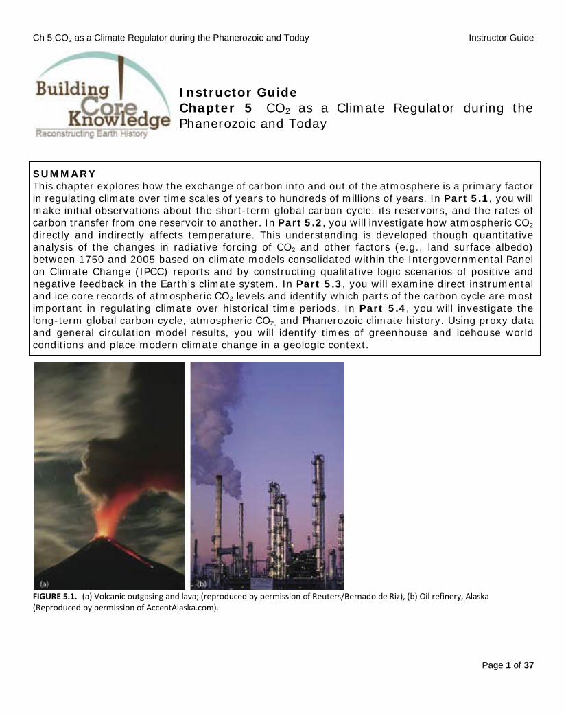
Instructor Guide Chapter 5 CO2 as a Climate Regulator during the Phanerozoic and Today

SUMMARY This chapter explores how the exchange of carbon into and out of the atmosphere is a primary factor in regulating climate over time scales of years to hundreds of millions of years. In Part 5.1, you will make initial observations about the short-term global carbon cycle, its reservoirs, and the rates of carbon transfer from one reservoir to another. In Part 5.2, you will investigate how atmospheric CO2 directly and indirectly affects temperature. This understanding is developed though quantitative analysis of the changes in radiative forcing of CO2 and other factors (e.g., land surface albedo) between 1750 and 2005 based on climate models consolidated within the Intergovernmental Panel on Climate Change (IPCC) reports and by constructing qualitative logic scenarios of positive and negative feedback in the Earth’s climate system. In Part 5.3, you will examine direct instrumental and ice core records of atmospheric CO2 levels and identify which parts of the carbon cycle are most important in regulating climate over historical time periods. In Part 5.4, you will investigate the long-term global carbon cycle, atmospheric CO2, and Phanerozoic climate history. Using proxy data and general circulation model results, you will identify times of greenhouse and icehouse world conditions and place modern climate change in a geologic context.

FIGURE 5.1. (a) Volcanic outgasing and lava; (reproduced by permission of Reuters/Bernado de Riz), (b) Oil refinery, Alaska (Reproduced by permission of AccentAlaska.com).


of 37

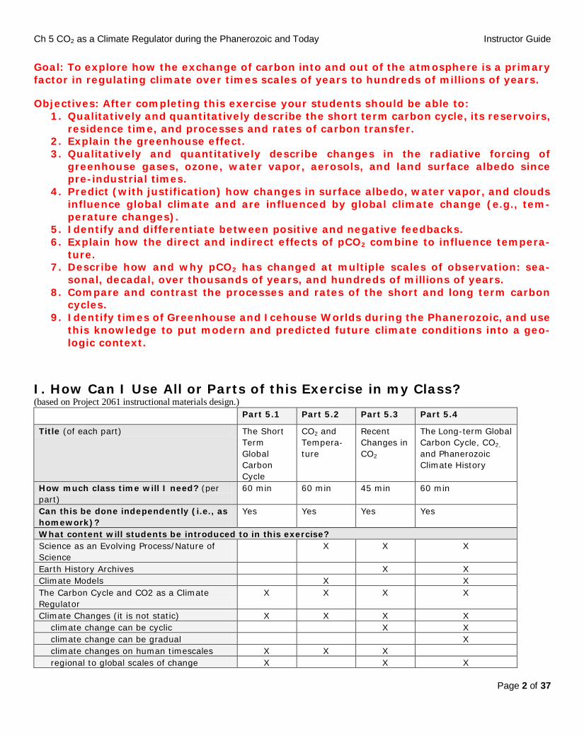
Goal: To explore how the exchange of carbon into and out of the atmosphere is a primary factor in regulating climate over times scales of years to hundreds of millions of years. Objectives: After completing this exercise your students should be able to:

1. Qualitatively and quantitatively describe the short term carbon cycle, its reservoirs, residence time, and processes and rates of carbon transfer.

2. Explain the greenhouse effect. 3. Qualitatively and quantitatively describe changes in the radiative forcing of

greenhouse gases, ozone, water vapor, aerosols, and land surface albedo since pre-industrial times.

4. Predict (with justification) how changes in surface albedo, water vapor, and clouds influence global climate and are influenced by global climate change (e.g., tem-perature changes).

5. Identify and differentiate between positive and negative feedbacks. 6. Explain how the direct and indirect effects of pCO2 combine to influence tempera-

ture. 7. Describe how and why pCO2 has changed at multiple scales of observation: sea-

sonal, decadal, over thousands of years, and hundreds of millions of years. 8. Compare and contrast the processes and rates of the short and long term carbon

cycles. 9. Identify times of Greenhouse and Icehouse Worlds during the Phanerozoic, and use

this knowledge to put modern and predicted future climate conditions into a geo-logic context.

I. How Can I Use All or Parts of this Exercise in my Class? (based on Project 2061 instructional materials design.) Part 5.1 Part 5.2 Part 5.3 Part 5.4

Title (of each part) The Short Term Global Carbon Cycle

CO2 and Tempera-ture

Recent Changes in CO2

The Long-term Global Carbon Cycle, CO2, and Phanerozoic Climate History

How much class time will I need? (per part)

60 min 60 min 45 min 60 min

Can this be done independently (i.e., as homework)?

Yes Yes Yes Yes

What content will students be introduced to in this exercise? Science as an Evolving Process/Nature of Science

X X X

Earth History Archives X X Climate Models X X The Carbon Cycle and CO2 as a Climate Regulator

X X X X

Climate Changes (it is not static) X X X X climate change can be cyclic X X climate change can be gradual X climate changes on human timescales X X X regional to global scales of change X X X


of 37

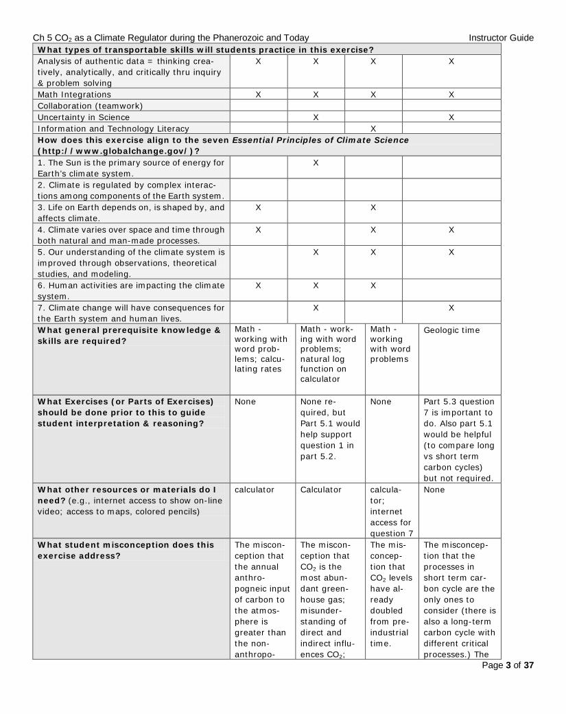
What types of transportable skills will students practice in this exercise? Analysis of authentic data = thinking crea-tively, analytically, and critically thru inquiry & problem solving

X X X X

Math Integrations X X X X Collaboration (teamwork) Uncertainty in Science X X Information and Technology Literacy X How does this exercise align to the seven Essential Principles of Climate Science (http://www.globalchange.gov/)? 1. The Sun is the primary source of energy for Earth’s climate system.

X

2. Climate is regulated by complex interac-tions among components of the Earth system.

3. Life on Earth depends on, is shaped by, and affects climate.

X X

4. Climate varies over space and time through both natural and man-made processes.

X X X

5. Our understanding of the climate system is improved through observations, theoretical studies, and modeling.

X X X

6. Human activities are impacting the climate system.

X X X

7. Climate change will have consequences for the Earth system and human lives.

X X

What general prerequisite knowledge & skills are required?

Math - working with word prob-lems; calcu-lating rates

Math - work-ing with word problems; natural log function on calculator

Math - working with word problems

Geologic time

What Exercises (or Parts of Exercises) should be done prior to this to guide student interpretation & reasoning?

None None re-quired, but Part 5.1 would help support question 1 in part 5.2.

None Part 5.3 question 7 is important to do. Also part 5.1 would be helpful (to compare long vs short term carbon cycles) but not required.

What other resources or materials do I need? (e.g., internet access to show on-line video; access to maps, colored pencils)

calculator Calculator calcula-tor; internet access for question 7

None

What student misconception does this exercise address?

The miscon-ception that the annual anthro-pogneic input of carbon to the atmos-phere is greater than the non- anthropo-

The miscon-ception that CO2 is the most abun-dant green-house gas; misunder-standing of direct and indirect influ-ences CO2;

The mis-concep-tion that CO2 levels have al-ready doubled from pre- industrial time.

The misconcep-tion that the processes in short term car-bon cycle are the only ones to consider (there is also a long-term carbon cycle with different critical processes.) The


of 37

genic (natural) input. The misconcep-tions that the biosphere is the largest reservoir of carbon and that most carbon in the lithosphere is in the form of oil or coal.

how human activities di-rectly affect temperature, water vapour, and land sur-face albedo. Misunder-standing of positive vs negative feedbacks.

misconception that we are cur-rently experiencing among the warmest times in Earth history.

What forms of data are used in this? (e.g., graphs, tables, photos, maps)

Complex conceptual diagram with quantitative data

Complex conceptual diagram with quantitative data; tables

Graphs Conceptual dia-gram; graphs

What geographic locations are these datasets from?

Global averages

Global aver-ages

Mauna Loa, Hawaii

Global; Antarc-tica;

How can I use this exercise to identify my students’ prior knowledge (i.e., student misconceptions, commonly held beliefs)?

Students will likely feel the most comfortable with Parts 1 and 3, so these help build a baseline to introduce the more complex (and perhaps more important) ideas in Parts 2 and 4. Some of the misconceptions identified are directly addressed with questions in the exercise parts.

How can I encouraging students to re-flect on what they have learned in this exercise? [Formative Assessment]

Each exercise part can be concluded by asking: On note card (with or without name) to turn in, answer: What did you find most interesting/helpful in the exercise we did above? Does what we did model scientific practice? If so, how and if not, why not?

How can I assess student learning after they complete all or part of the exercise? [Summative Assessment]

See suggestions in Summative Assessment section below.

Where can I go to for more information on the science in this exercise?

See the supplemental materials and reference sections below.

II. Annotated Student Worksheets (i.e., the ANSWER KEY)

This section includes the annotated copy of the student worksheets with answers for each Part of this Chapter. This instructor guide contain the same sections as in the student book chapter, but also includes additional information such as: useful tips, discussion points, notes on places where students might get stuck, what specific points students should come away with from an exercise so as to be prepared for further work, as well as ideas and/or material for mini-lectures.


of 37

Part 5.1. The Short-Term Global Carbon Cycle

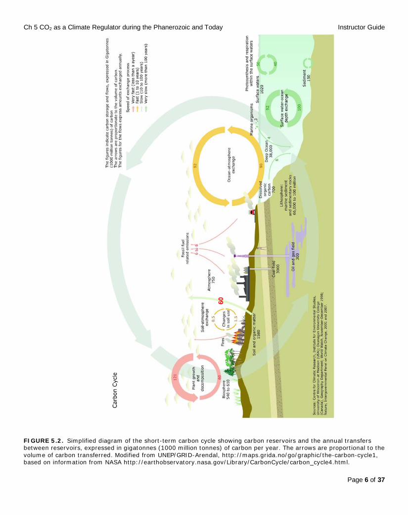
Introduction Examine the carbon cycle diagram (Figure 5.2). You can consider this to be a modern snapshot of the major reservoirs in which carbon is stored, the processes that transfer carbon between those reservoirs each year, and the rates at which that carbon is transferred from one reservoir to an-other in the Earth’s system. The major carbon reservoirs in the Earth’s system are the atmos-phere, the terrestrial biosphere, soil, the oceans (including surface waters, deep waters, and the marine biosphere), and the lithosphere (including carbon in sediments and rocks, and fossil fuels). IMPORTANT CORRECTION to FIGURE 5.2 (p. 171): An important label was omitted from Figure 5.2 and must be added for students to calculate reservoir time (question 4): On Figure 5.2, the light green arrow representing soil-atmosphere exchange of carbon should be labelled with the number "60". [The base of the arrow is right next to the label soil and organic matter.] Please tell your students to make this correction.

1 Using data from Figure 5.2 compare the relative size of each of the five major carbon reservoirs of the Earth’s system by listing the reservoirs in rank order from largest to smallest in column 2 of Table 5.1. From Figure 5.2, the “ocean” reservoir includes “dissolved organic carbon”, the “deep ocean”, the “surface waters”, and “marine organisms”. The “lithosphere” reservoir includes “ma-rine sediment and sedimentary rocks”, “sediments”, “oil and gas field”, and “coalfield”. See answers in Table 5.1. This should be fairly straightforward as long as students read intro-

ductory paragraph which defines the reservoirs, and the question which lists out the reservoirs and their subcategories. Students will likely be surprised about the rank order with the terrestrial biosphere being the smallest reservoir, and the lithosphere being the largest (this will be explored more in Part 5.4). You may wish to discuss that terrestrial carbon is transferred and can build up in the soil, just as carbon in the surface ocean is transferred and builds up in the deep ocean.


of 37

FIGURE 5.2. Simplified diagram of the short-term carbon cycle showing carbon reservoirs and the annual transfers between reservoirs, expressed in gigatonnes (1000 million tonnes) of carbon per year. The arrows are proportional to the volume of carbon transferred. Modified from UNEP/GRID-Arendal, http://maps.grida.no/go/graphic/the-carbon-cycle1, based on information from NASA http://earthobservatory.nasa.gov/Library/CarbonCycle/carbon_cycle4.html.

60


of 37

TABLE 5.1. Carbon Cycle Reservoirs

Column 1 Relative

Size

Column 2 Reservoir Name

Column 3 Form(s) of Carbon in

Reservoir

1 (largest) Lithosphere (69,450 to 100,003,450 gigatons)

Largely solid in minerals in rocks (e.g., calcite in limestone, mar-ble) and in sediment. Also as a liquid in oil, and a gas in natural gas.

2 Ocean (39723 gigatons) Dissolved ions (e.g., CO32-,

HCO3-, H2CO3) and gases (CO2) in

sea water; as marine life (algae [foram and coccoliths if they remember back to chapter 3; seaweed], animals [fish; coral reefs], coastal plants [marsh grass])

3 Soil (1580 gigatons) As solid forms (e.g., minerals and rock fragments), and in dead and decaying organic matter (e.g., leaf litter) and living organisms in soil (e.g., bacteria, worms). Also as dissolved forms in water and gases in pore spaces.

4 Atmosphere (750 gigatons) Largely as CO2 and CH4 gases.

5 (smallest)

Terrestrial Biosphere (540 to 610 gigatons)

In organic forms – living animal and plant matter.

A follow-up assignment could be to have student calculate the percent of the total carbon reservoir that each of the 5 reservoirs in Table 5.1 makes-up. For example using the highest estimates the terrestrial biosphere is: (610/100,046,113)*100 = .0006% of the total carbon reservoir.


of 37

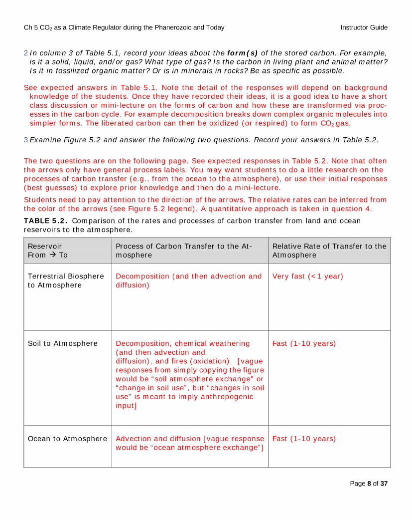
2 In column 3 of Table 5.1, record your ideas about the form(s) of the stored carbon. For example, is it a solid, liquid, and/or gas? What type of gas? Is the carbon in living plant and animal matter? Is it in fossilized organic matter? Or is in minerals in rocks? Be as specific as possible.

See expected answers in Table 5.1. Note the detail of the responses will depend on background knowledge of the students. Once they have recorded their ideas, it is a good idea to have a short class discussion or mini-lecture on the forms of carbon and how these are transformed via proc-esses in the carbon cycle. For example decomposition breaks down complex organic molecules into simpler forms. The liberated carbon can then be oxidized (or respired) to form CO2 gas.

3 Examine Figure 5.2 and answer the following two questions. Record your answers in Table 5.2.

The two questions are on the following page. See expected responses in Table 5.2. Note that often the arrows only have general process labels. You may want students to do a little research on the processes of carbon transfer (e.g., from the ocean to the atmosphere), or use their initial responses (best guesses) to explore prior knowledge and then do a mini-lecture.

Students need to pay attention to the direction of the arrows. The relative rates can be inferred from the color of the arrows (see Figure 5.2 legend). A quantitative approach is taken in question 4.

TABLE 5.2. Comparison of the rates and processes of carbon transfer from land and ocean reservoirs to the atmosphere.

Reservoir From To

Process of Carbon Transfer to the At-mosphere

Relative Rate of Transfer to the Atmosphere

Terrestrial Biosphere to Atmosphere

Decomposition (and then advection and diffusion)

Very fast (<1 year)

Soil to Atmosphere Decomposition, chemical weathering (and then advection and diffusion), and fires (oxidation) [vague responses from simply copying the figure would be “soil atmosphere exchange” or “change in soil use”, but “changes in soil use” is meant to imply anthropogenic input]

Fast (1-10 years)

Ocean to Atmosphere Advection and diffusion [vague response would be “ocean atmosphere exchange”]

Fast (1-10 years)


of 37

Reservoir From To

Process of Carbon Transfer to the At-mosphere

Relative Rate of Transfer to the Atmosphere

Lithosphere to Atmosphere*

volcanism n/a (because the processes are so slow that they are not shown on this diagram; this becomes an important process in the long term carbon cycle see Part 5.4)

* This row is completed for you because the natural process of carbon transfer from the lithosphere to the atmosphere via volcanism is so slow they are not included in the short term carbon cycle (Figure 5.2). However, note that volcanism will be an important process of the long-term carbon cycle which is introduced in Part 5.4.

(a) What are the natural processes that transfer carbon to the atmosphere?

See Table 5.2.

(b) What are relative rates [i.e., very fast (<1 yr), fast (1–10 yrs), slow (10–100 yrs), or very slow (>100 yrs)] of natural (non-anthropogenic) carbon transfer to the atmosphere?

See Table 5.2

Another way to consider the rate at which each carbon reservoir is affected by these processes is to calculate the average amount of time that an atom of carbon spends in that reservoir. This is known as the residence time for that reservoir. Under steady state conditions, the residence time is constant, because the input and output rates are equal. However, steady state conditions are not always the case in nature. An estimate of the residence time can be calculated by dividing the total amount of carbon in that reservoir by the rate at which carbon is added or removed each year.

4 Using data from Figure 5.2 complete Table 5.3 in order to estimate the residence times of carbon in the atmosphere, surface ocean, terrestrial biosphere, and soil owing to natural processes only. Use the rates at which carbon is added to the reservoir of interest each year for these calculations.

An important label was omitted from Figure 5.2 and must be added for students to calculate reservoir time (question 4): On Figure 5.2, the light green arrow representing soil-atmosphere exchange of carbon should be labelled with the number "60". [The base of the arrow is right next to the label soil and organic matter.] Please tell your students to make this correction.

See answers in Table 5.3. Students may need reminding that they have to pay attention to the direction of the arrows in Figure 5.2. Also they may have questions as to why for example plant growth and decomposition (biosphere exchange with atm) are not the same number; this is because not all of the carbon produced from in plant growth is returned directly to the atmosphere, much of it is instead transferred to soil.


of 37

TABLE 5.3. Residence time of carbon in different reservoirs

Reservoir Addition Process

Amount Added (Gigatonnes/yr)

Total Added (Gigaton-nes/yr)

Total in Reservoir (Gigatonnes)

Residence Time (yrs)

Atmosphere Plant Decomposition

60 210 See Table 5.2 or Fig. 5.2 to complete this column. 750

3.6

Soil– atmosphere ex-change [this is the long green arrow, not the human- caused changes in land-use]

60

Ocean– atmosphere exchange

90

Surface Ocean [not the total ocean – just sur-face ocean because we are focusing on the ocean- atmosphere exchange which takes place in the surface waters]

Ocean– atmosphere exchange

92 92 1020 [note: this is just the surface ocean value not the total ocean value]

11.1

Terrestrial biosphere

Plant growth 121 121 540 to 610 (average 575)

4.8

Soil Addition from vegetation: cal-culate this as the difference be-tween “plant growth” and “plant decomposi-tion”

61 [note: students might include the 0.5 from atm to soil exchange, but this is attributed to anthropogenic sources]

61 1580 25.9

5 What are the two primary anthropogenic processes shown in Figure 5.2 that affect the carbon cycle?

Fossil fuel related emissions and changes in soil use (+ fires).


of 37

6 (a) Using data in Figure 5.2, calculate the total amount of carbon transferred to the atmosphere each year from anthropogenic processes. Show your work.

Fossil fuel use (6 to 8 gigatons/year) + changes in soil use (1.5 gigatons/year) = 7.5 to 9.5 gi-gatons/year

(b) Do anthropogenic (see question 6a) or natural (see Table 5.3) processes transfer more carbon to the atmosphere each year?

Natural processes by far; the natural input to the atmosphere is 210 gigatons/year; compared to the 7.5 to 9.5 gigatons/year from anthropogenic sources. This might surprise students, the an-thropogenic input is not that large overall, but that doesn’t mean it is insignificant - see next question.

(c) If the amount of carbon transferred out of the atmosphere does not change, what effects will anthropogenic activity have on the total amount of carbon in the atmospheric reservoir over time?

The total amount of carbon in the atmospheric reservoir will increase over time.

Part 5.2. CO2 and Temperature

The Greenhouse Effect The transfer of carbon to and from the atmosphere is a primary factor in regulating climate over time scales of years to hundreds of millions of years. This is because two of the atmospheric greenhouse gases with the greatest influence on Earth’s surface temperature are carbon compounds: carbon dioxide (CO2) and methane (CH4). Other important greenhouse gases include stratospheric water vapor (H2O), nitrous oxide (N2O), ozone (O3), and halocarbons (e.g., chlorofluorocarbons, CFCs).

1 Read the box below on the greenhouse effect and think about the carbon cycle. If the amount of carbon added to the atmosphere is greater than the amount of carbon removed from the at-mosphere, how would you expect Earth’s surface temperature to change? Explain.

Assuming the carbon added to the atmosphere would be in the form of CO2 or CH4, then the temperature should increase because these are greenhouse gases, which absorb the back ra-diation from the Earth and reradiate it, increasing the temperature of the lower atmosphere and the surface of the Earth. Some students might assume the carbon is in the form of black soot that could then fall out of the atmosphere onto snow (see figure). This would also increase tem-perature because of the resulting darker surface, decreasing albedo and increasing surface heat absorption.


of 37

THE GREENHOUSE EFFECT Energy from the Sun is the primary driver of the Earth’s climate system. Energy travels through space as electromagnetic radiation, in the form of electromagnetic waves with a wide range of wavelengths. However, the heat energy that drives the Earth’s climate system is only a narrow spectrum of relatively short wavelengths of this broad electromagnetic spectrum; the important radiation on the Earth is predominantly visible light, which has a relatively short wavelength and is used by plants, algae, and other organisms to drive photosynthesis.

Because the the Earth gains heat from the Sun and has a temperature above absolute zero (−273°C or 0K), the Earth radiates heat to its surroundings. Because of the temperature of the Earth (averaging 15–16°C), the energy released by the Earth to its atmosphere (also known as the Earth’s back radiation) has a longer wavelength than the incoming visible radiation from the Sun. This back radiation is also known as longwave radiation.

Some gases absorb the longwave radiation emitted by the Earth and re-radiate that energy, providing additional warming of the atmosphere and Earth’s surface. This greenhouse effect is what makes the Earth habitable; without out it, the Earth’s surface temperature would be on average 31°C cooler, well below the freezing temperature of water. Clearly the greenhouse effect is essential for life as we know it on Earth, although too much of a “good” thing can also have serious reper-cussions!

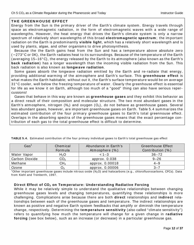
Gases that behave in this way are known as greenhouse gases and they exhibit this behavior as a direct result of their composition and molecular structure. The two most abundant gases in the Earth’s atmosphere, nitrogen (N2) and oxygen (O2), do not behave as greenhouse gases. Several less abundant gases, however, are important greenhouse gases on Earth. Table 5.4 summarizes the estimated contribution of the four primary greenhouse gases to Earth’s total greennouse effect. Overlaps in the absorbing spectra of the greenhouse gases means that the exact percentage con-tribution of each gas to the total greenhouse effect is difficult to determine.

TABLE 5.4. Estimated contribution of the four primary individual gases to Earth’s total greenhouse gas effect

Gas1 Chemical Formula

Abundance in Earth’s Atmosphere (%)

Greenhouse Effect Contribution (%)

Water Vapor H2O <1–3 36–72 Carbon Dioxide CO2 approx. 0.038 9–26 Methane CH4 approx. 0.00018 4–9 Ozone O3 approx. 0.00006 3–7 1Other important greenhouse gases include nitrous oxide (N2O) and halocarbons (e.g., chlorofluorocarbons, CFCs). Data from Kiehl and Trenberth, 1997.

Direct Effect of CO2 on Temperature: Understanding Radiative Forcing While it may be relatively simple to understand the qualitative relationships between changing greenhouse gases levels and changing temperatures, quantifying these relationships is more challenging. Complications arise because there are both direct relationships and indirect rela-tionships between each of the greenhouse gases and temperature. The indirect relationships are known as positive and negative Earth system feedbacks that amplify or diminish the temperature change, respectively. Determining the temperature sensitivity (also called “climate sensitivity”) refers to quantifying how much the temperature will change for a given change in radiative forcing (see box below), such as an increase (or decrease) in a particular greenhouse gas.


of 37

RADIATIVE FORCING (RF) Radiative forcing is a measure of the change in the direct influence that a factor has in altering the balance of incoming and outgoing energy in the Earth–atmosphere system. It is used to rank quantitatively the importance of climate change factors (Figure 5.3). Radiative forcing does not take into account indirect influences on climate (i.e., Earth system feedbacks). The unit for radiative forcing is watts per square meter (W/m2), the same unit used to measure incoming solar radiation (“insolation”) and Earth’s back radiation. Positive forcing increases surface tem-perature, whereas negative forcing cools it. The radiative forcing of any gas is determined from atmospheric radiative transfer models. It is calculated by taking the natural logarithm of the change in that gas concentration (ppm) and mul-tiplying by a gas-dependent constant. For example the following formula is used to calculate the radiative forcing of CO2:

RF = 5.35 * ln Present concentration of CO2

Initial concentration of CO2

(RF discussion adapted from Forster et al., 2007; RF calculation from http://www.esrl.noaa.gov/gmd/aggi/)

FIGURE 5.3. Anthropogenic (human) and natural radiative forcing terms that affect climate change over a 255-yr window, from 1750 to 2005. Uncertainties are represented by the thin black lines. From Forster et al., 2007.


of 37

2 Measurements of the trapped atmospheric gas in ice cores indicate that the 1750 (pre-industrial) concentration of atmospheric CO2 was 280 ppm. CO2 concentrations have been directly measured from the atmosphere since 1959 at the NOAA Mauna Loa Observatory in Hawaii. The 2005 concentration of CO2 was 378 ppm. The 2011 concentration of CO2 was >392 ppm and it continues to rise.

Calculate the radiative forcing of CO2 on climate from 1750 to 2005 using the equation in the box above. Show your work.

5.35 ln (378/280) = 1.6 W/m2

3 How does your answer to Question 2 compare to the radiative forcing of CO2 from 1750 to 2005 as reported in Figure 5.3?

Should be the same

4 Which radiative forcing term had the highest radiative forcing from 1750 to 2005, based on the data in Figure 5.3?

Atmospheric CO2 specifically, or long-lived Greenhouse gases more generally.

Note some additional questions that you can use to explore student’s understanding of the data in Figure 5.3 are:

• Which radiative forcing term has the lowest uncertainty (i.e., highest confidence) in the

measurements? Uncertainty is shown with the horizontal black lines in the figure. The RF factor with the lowest uncertainty (highest confidence) is the calculation of linear contrails (essentially artificial clouds from jets).

• Would positive

radiative forcing increase or decrease Earth’s surface temperature? Explain. [Note radiative forcings ≠ feedbacks.]

Positive RF means greater W/m2 in Earth’s climate system, this additional “heat energy” would increase Earth’s surface temperature.

• Overall did the estimated direct effect

of human activities on climate cause warming or cooling between 1750 and 2005?

Need to look at bottom row of figure “total net of human activities”, which shows an increase in RF of +1.6 W/m2 between 1750 and 2005 (the range of estimated values is from wide however: +0.6 to +2.4 W/m2.), so overall effect is warming.

A NOTE ON WATER VAPOR


of 37

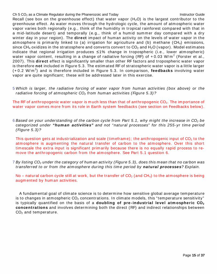
Recall (see box on the greenhouse effect) that water vapor (H2O) is the largest contributor to the greenhouse effect. As water moves through the hydrologic cycle, the amount of atmospheric water vapor varies both regionally (e.g., think of the humidity in tropical rainforest compared with that in a mid-latitude desert) and temporally (e.g., think of a humid summer day compared with a dry winter day in your region). The direct impact of human activity on the levels of water vapor in the atmosphere is primarily linked to (a) irrigation for agriculture and (b) methane (CH4) emissions, since CH4 oxidizes in the stratosphere and converts convert to CO2 and H2O (vapor). Model estimates indicate that regional irrigation produces ≤1% change in tropospheric (i.e., lower atmospheric) water vapor content, resulting in a change of radiative forcing (RF) of +0.03 W/m2 (Forster et al., 2007). This direct effect is significantly smaller than other RF factors and tropospheric water vapor is therefore not included in Figure 5.3. The estimated RF of stratospheric water vapor is a little larger (+0.2 W/m2) and is therefore included in Figure 5.3. In comparison, feedbacks involving water vapor are quite significant; these will be addressed later in this exercise.

5 Which is larger, the radiative forcing of water vapor from human activities (box above) or the radiative forcing of atmospheric CO2 from human activities (Figure 5.3)?

The RF of anthropogenic water vapor is much less than that of anthropogenic CO2. The importance of water vapor comes more from its role in Earth system feedbacks (see section on Feedbacks below).

6 Based on your understanding of the carbon cycle from Part 5.1, why might the increase in CO2 be categorized under “human activities” and not “natural processes” for this 255-yr time period (Figure 5.3)?

This question gets at industrialization and scale (timeframe); the anthropogenic input of CO2 to the atmosphere is augmenting the natural transfer of carbon to the atmosphere. Over this short timescale the extra input is significant primarily because there is no equally rapid process to re-move the anthropogenic carbon from the atmosphere. See Part 5.1 question 6.

7 By listing CO2 under the category of human activity (Figure 5.3), does this mean that no carbon was

transferred to or from the atmosphere during this time period by natural processes? Explain.

No – natural carbon cycle still at work, but the transfer of CO2 (and CH4) to the atmosphere is being augmented by human activities.

A fundamental goal of climate science is to determine how sensitive global average temperature is to changes in atmospheric CO2 concentrations. In climate models, this “temperature sensitivity” is typically quantified on the basis of a doubling of pre-industrial level atmospheric CO2 concentrations and involves determining both the direct (RF) and indirect relationships between CO2 and temperature.


of 37

8 What would the RF of CO2 be if the atmospheric level of CO2 rose to twice its pre-industrial level? Show your work. (Hint: refer back to question 2, Part 5.2.)

From question 2 Part 5.2, we recall that measurements of the trapped atmospheric gas in ice cores indicate that the 1750 (pre-industrial) concentration of atmospheric CO2 was 280 ppm. Therefore doubling that is 560 ppm. Thus,

5.35 ln (560/280) = 3.7 W/m2

Note that at this point we have not yet related RF to a specific change in temperature. This will be addressed in the later sections on (a) Indirect Effects of CO2 on Temperature: Earth System Feedbacks and (b) Combined Effect (Direct and Indirect) of CO2 on Temperature.

LAND SURFACE ALBEDO: A DIFFERENT STORY OF RADIATIVE FORCING While CO2 has a high radiative forcing and is therefore an important factor in directly regulating atmospheric temperature, it is not the only factor. For example, land surface albedo also affects atmospheric temperature. Albedo is a measure of the reflectivity of a surface. Lighter surfaces (e.g., fresh snow and ice) are more reflective (i.e., have a higher albedo) than darker surfaces (e.g., road pavement, dark soil, forests, lakes, and the ocean). The more reflective the surface, the less in-coming solar radiation is absorbed by that surface.

Model estimates indicate a decrease in the radiative forcing of the land surface albedo between 1750 and 2005 (Figure 5.3). In other words, the land surface was absorbing less (and reflecting more) incoming solar radiation in 2005 than in 1750 (i.e., the land surface albedo increased). It is important to understand that changes in snow and ice cover caused by the Earth system feedback were not factored in this calculation, since such changes would be indirect and ra-diative forcing is a measure of only direct effects on energy transfer in the Earth–atmosphere system.

9 Read the box on Land Surface Albedo. What direct changes in land use could cause land surface albedo to increase? If possible, provide examples of changing land use in your own region or state that might affect the reflectivity of the local land surface.

Changes in snow and ice cover are excluded in most of the RF models used by the IPCC, because the RF is only for direct effects (not indirect effects from changes in snow and ice coverage). Changes in the distribution of agriculture, pasture land, and forests are the primary cause of the increase in land surface albedo, according to the IPCC (Forester et al., 2007). The albedo of crop land can be much higher than that of forested land. In 1750, 6-7% of the total land surface was used for agriculture or pastures. In 1990, this was elevated to 35-39% of the total land surface (Forester et al., 2007 and references therein). Urbanization would presumably also affect albedo, however this was not discussed directly in the IPCC report (although the heat island effect of cities was discussed; Forester et al., 2007).

Humans may also have altered the reflective properties of snow and ice because of carbon soot deposits (pollution) on these white surfaces, and because of snow and ice melting. However, it is important to remember that ice melting can change the ice thickness (with little effect on surface albedo), as well as the geographic extent of the ice (affecting surface albedo).


of 37

Indirect Effects of CO2 on Temperature: Earth System Feedbacks In general, as radiative forcing increases, the Earth’s average temperature also increases. How-ever, the relationship between a change in radiative forcing and the corresponding change in temperature is not simple or straightforward. It is calculated within large scale computer models of the Earth’s atmosphere, called general circulation models (GCMs). In general, GCM results indicate that the direct effect of doubling CO2 would produce an increase in radiative forcing of 3.7 W/m2 (refer back to Question 8) and an increase in global average temperature of approximately 1.25°C (Rahmstorf, 2008; Ruddiman, 2008).

This is not the only way that changing CO2 levels affect temperature. There are also indirect effects on other parts of the Earth system, which in turn either augment (positive feedback) or diminish (negative feedback) the direct effect that CO2 has on temperature. These earth system feedbacks include: (a) water vapor, (b) surface albedo, and (c) clouds. To determine qualitatively how these Earth system feedbacks affect temperature, consider Table 5.5.

TABLE 5.5. Earth System Feedback Factors

Feedback Key Physical Relationships/Conditions Water Vapor 1 A warmer atmosphere can store more water vapor than a colder atmosphere.

[This is based on the Clausius–Clapeyron relationship between temperature and saturation vapor pressure].

2 A warmer atmosphere will evaporate more water from the ocean, which increases the amount of water vapor in the atmosphere.

3 Water vapor is a greenhouse gas. Surface Albedo

4 Albedo is a measure of the reflectivity of a surface. 5 Lighter surfaces (e.g., fresh snow and ice) are more reflective (have a higher

albedo) than darker surfaces (e.g., road pavement, dark soil, forests, lakes, ocean).

6 The more reflective the surface, the less incoming solar radiation is absorbed by that surface.

Clouds 7 Clouds vary in space (altitude, latitude, longitude) and time. Cloud cover, height, albedo, water content, and particle size all affect cloud feedbacks.

8 A warmer atmosphere evaporates more water from the ocean, thereby supplying more moisture to the atmosphere. A warmer atmosphere also can store more water vapor than a cold atmosphere, thereby reducing condensation. Both of these factors affect the abundance, type, and size of clouds.

9 Cloud thickness increases with temperature. 10 The upper surface of some clouds reflects incoming solar radiation; these have a

high albedo. Other clouds are less reflective and therefore have only a moderate albedo.

11 The lower surface of some clouds re-radiates long wavelength radiation from the Earth.

12 Higher clouds are colder and therefore radiate less long wavelength energy back to space [i.e., Stefan–Boltzmann relationship].


of 37

10 With the information from Table 5.5 in mind, complete the blanks in each of the following six feedback scenarios and justify the selections you make. In each case, indicate how each of the feedback factors will change (will it increase or will it decrease?) and how the resulting tem-perature will change (will it increase or will it decrease?). For each scenario indicate whether it outlines a positive (P) or negative (N) feedback.

(a) Atmospheric CO2 increases temperature increases water vapor increases tem-perature increases. P or N? positive

Justification: See Table 5.5, key physical relationships and conditions 1, 2, 3 (esp. 2 & 3).

(b) Atmospheric CO2 increases temperature increase snow and ice decrease surface albedo decreases temperature increases. P or N? positive


(C) NOTE: the feedbacks that involve clouds are very challenging. Depending on their reasoning, students could have different answers. Included below are two responses that may be most common; scenario C1 is more likely than C2. To grade these it is more important to determine if the logic is internally consistent and if a reasonable justification is provided.

(c1) Atmospheric CO2 increases temperature increases clouds increase tempera-ture decreases. P or N? negative

Justification: From Table 5.5 the cloud relationships and conditions are mainly items 7-12. However, it is also critical to go back to water vapour because if there is more water vapour there will likely be more clouds (assuming particulate matter for condensation nuclei, and in comparison to a drier atmosphere), and if we assume

(c2) Atmospheric CO2 increases temperature increases clouds decrease tem-perature increases. P or N? positive

the clouds are light colored then they will be reflective.

Justification: From Table 5.5 the cloud relationships and conditions are mainly items 7-12. However, critical to this logic scenario is the second part of item 7 (Table 5.5; warmer atmosphere can store more water vapour

(d) Atmospheric CO2 decreases temperature decreases water vapor decreases tem-perature decreases. P or N? postive

, but rate of condensation is reduced compared to a cooler atmos-phere). Water vapour is needed to form the clouds.


(e) Atmospheric CO2 decreases temperature decreases snow and ice increase surface albedo increases temperature decreases. P or N? positive



of 37

(F) Note: we have the same complications as for letter C above, the most likely responses are shown below. (Scenario F1 is more likely than F2):

(f1) Atmospheric CO2 decreases temperature decreases clouds decrease temperature increases. P or N? negative

Justification: From Table 5.5 the cloud relationships and conditions are mainly items 7-12. How-ever, it is critical to think of the water vapour feedback conditions as well, in particular that lower temperatures probably mean less water vapour and then fewer clouds (in comparison to a wetter atmosphere), and fewer clouds probably means more incoming radiation absorbed than reflected.

(f2) Atmospheric CO2 decreases temperature decreases clouds increase temperature-decreases. P or N? positive

Justification: From Table 5.5 the cloud relationships and conditions are mainly items 7-12. How-ever, critical to this logic scenario is the second part of item 7 (Table 5.5; cooler atmosphere can store less water vapour, but rate of condensation is greater compared to a warmer atmosphere

11 Based on your responses to the six scenarios in Question 10, which of these feedbacks in-troduces the most uncertainty in predicting its ultimate effect on Earth’s climate? Why might that be?

).

Cloud feedbacks (letters c and f above) because there are many different conflicting properties of clouds and very changeable clouds conditions (e.g., types, heights, and thicknesses of clouds).

Combined Effect (Direct and Indirect) of CO2 on Temperature In the same way that you have identified uncertainties in your qualitative predictions, each GCM identifies uncertainties and has its own way of dealing with those uncertainties in its calculations. As a result, different GCMs often predict different temperature changes for the same change in the concentration of atmospheric CO2.

From the range of GCM results, the “average”, or mid-range, model projections for a doubling of CO2 are:

• an increase of approximately 2.5°C caused by the water vapor feedback, • an increase of approximately 0.6°C caused by the surface albedo feedback (including snow

and ice albedo changes), and • a decrease of approximately 1.85°C caused by the cloud feedback (Ruddiman, 2008).

12 Calculate the projected combined effect of these three climate system feedbacks on tem-perature, given a doubling of CO2. Show your work.

2.5ºC + 0.6ºC - 1.85ºC = a warming of 1.25ºC

13 As stated earlier, the direct radiative effect of doubling the pre-industrial level of CO2 is 3.7 W/m2, resulting in an increase of global average temperature of 1.25°C (Rahmstorf 2008; Rud-diman 2008). Calculate the projected total warming caused by this direct radiative effect plus the warming from the climate system feedbacks (from questions 12) when CO2 is doubled?

1.25ºC + 1.25ºC = 2.5ºC


of 37

Part 5.3. Recent Changes in CO2

Consider the atmospheric CO2 data from air samples collected at Mauna Loa Observatory for the period 1958–2010 (Figure 5.4).

1 Is this carbon dioxide record a direct measure of carbon dioxide concentrations in our atmos-phere or is it a proxy (indirect indicator) of carbon dioxide concentrations?

Directly measured

FIGURE 5.4. Atmospheric CO2 concentrations measured at Mauna Loa Observatory, Hawaii. From: Dr. Pieter Tans, NOAA/ESRL, www.esrl.noaa.gov/gmd/ccgg/trends/. CORRECTION: Horizontal axis of graph should be Year (not Yaer)

2 What do you think the solid black curve represents?

Mean trend line (annual average).

3 What do you think the red saw-toothed curve represents?

Fluctuations in a CO2 data, with samples taken at multiple times throughout the year.

4 How many peaks (or “teeth”) are present in a 5-year interval on the saw-toothed curve? Based on

http://www.esrl.noaa.gov/gmd/ccgg/trends/�


of 37

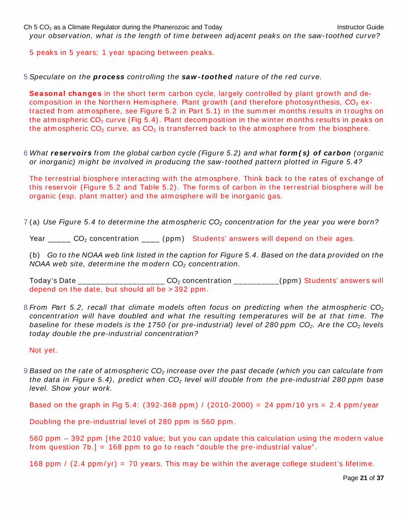
your observation, what is the length of time between adjacent peaks on the saw-toothed curve?

5 peaks in 5 years; 1 year spacing between peaks.

5 Speculate on the process controlling the saw-toothed nature of the red curve.

Seasonal changes in the short term carbon cycle, largely controlled by plant growth and de-composition in the Northern Hemisphere. Plant growth (and therefore photosynthesis, CO2 ex-tracted from atmosphere, see Figure 5.2 in Part 5.1) in the summer months results in troughs on the atmospheric CO2 curve (Fig 5.4). Plant decomposition in the winter months results in peaks on the atmospheric CO2 curve, as CO2 is transferred back to the atmosphere from the biosphere.

6 What reservoirs from the global carbon cycle (Figure 5.2) and what form(s) of carbon (organic or inorganic) might be involved in producing the saw-toothed pattern plotted in Figure 5.4?

The terrestrial biosphere interacting with the atmosphere. Think back to the rates of exchange of this reservoir (Figure 5.2 and Table 5.2). The forms of carbon in the terrestrial biosphere will be organic (esp. plant matter) and the atmosphere will be inorganic gas.

7 (a) Use Figure 5.4 to determine the atmospheric CO2 concentration for the year you were born?

Year _____ CO2 concentration ____ (ppm) Students’ answers will depend on their ages.

(b) Go to the NOAA web link listed in the caption for Figure 5.4. Based on the data provided on the NOAA web site, determine the modern CO2 concentration.

Today’s Date ___________________ CO2 concentration __________(ppm) Students’ answers will depend on the date, but should all be >392 ppm.

8 From Part 5.2, recall that climate models often focus on predicting when the atmospheric CO2 concentration will have doubled and what the resulting temperatures will be at that time. The baseline for these models is the 1750 (or pre-industrial) level of 280 ppm CO2. Are the CO2 levels today double the pre-industrial concentration?

Not yet.

9 Based on the rate of atmospheric CO2 increase over the past decade (which you can calculate from the data in Figure 5.4), predict when CO2 level will double from the pre-industrial 280 ppm base level. Show your work.

Based on the graph in Fig 5.4: (392-368 ppm) / (2010-2000) = 24 ppm/10 yrs = 2.4 ppm/year

Doubling the pre-industrial level of 280 ppm is 560 ppm.

560 ppm – 392 ppm [the 2010 value; but you can update this calculation using the modern value from question 7b.] = 168 ppm to go to reach “double the pre-industrial value”.

168 ppm / (2.4 ppm/yr) = 70 years. This may be within the average college student’s lifetime.


of 37

Now consider the atmospheric CO2 data for the last 20,000 years, measured from bubbles of trapped gas in ice cores and directly from the atmosphere (Figure 5.5).

FIGURE 5.5. Atmospheric CO2 concentrations over the last 20,000 years. The area of gray shading indicates pre-industrial natural range of CO2. Data are from ice cores (colored symbols are from different studies), atmospheric samples (colored bars), and merged (spline function; black). The corresponding radiative forcing relative to pre-industrial (1780 baseline) levels are shown on the right axis of the large panel. From Joos and Spahni, 2008. Note that approximately 260 years ago (1750) the CO2 level was 280 ppm.

10 The last glacial maximum occurred approximately 20,000 years ago. At this time continental ice sheets were widespread, covering much of the landscape north of 40°N (e.g., southern Ohio). What was the atmospheric CO2 concentration during the last glacial maximum (Figure 5.5)?

~192 ppm

11 Describe the trends of CO2 over the last 20,000 years (Figure 5.5). In particular, identify times when the slope of the CO2 trend changed noticeably.

20,000 yr ago to 17,500 yrs ago: fairly steady at ~192 ppm

17,500 yrs ago to 14,000 yrs ago: rapid increase to ~240 ppm

14,000 yrs ago to 12,000 yrs ago: fairly steady at ~240 ppm (or slight lowering of CO2)

12,000 yrs ago to ~10,000 yrs ago: rapid increase to 265 ppm

10,000 yrs ago to ~7500 yrs ago: slight decrease to ~260 ppm


of 37

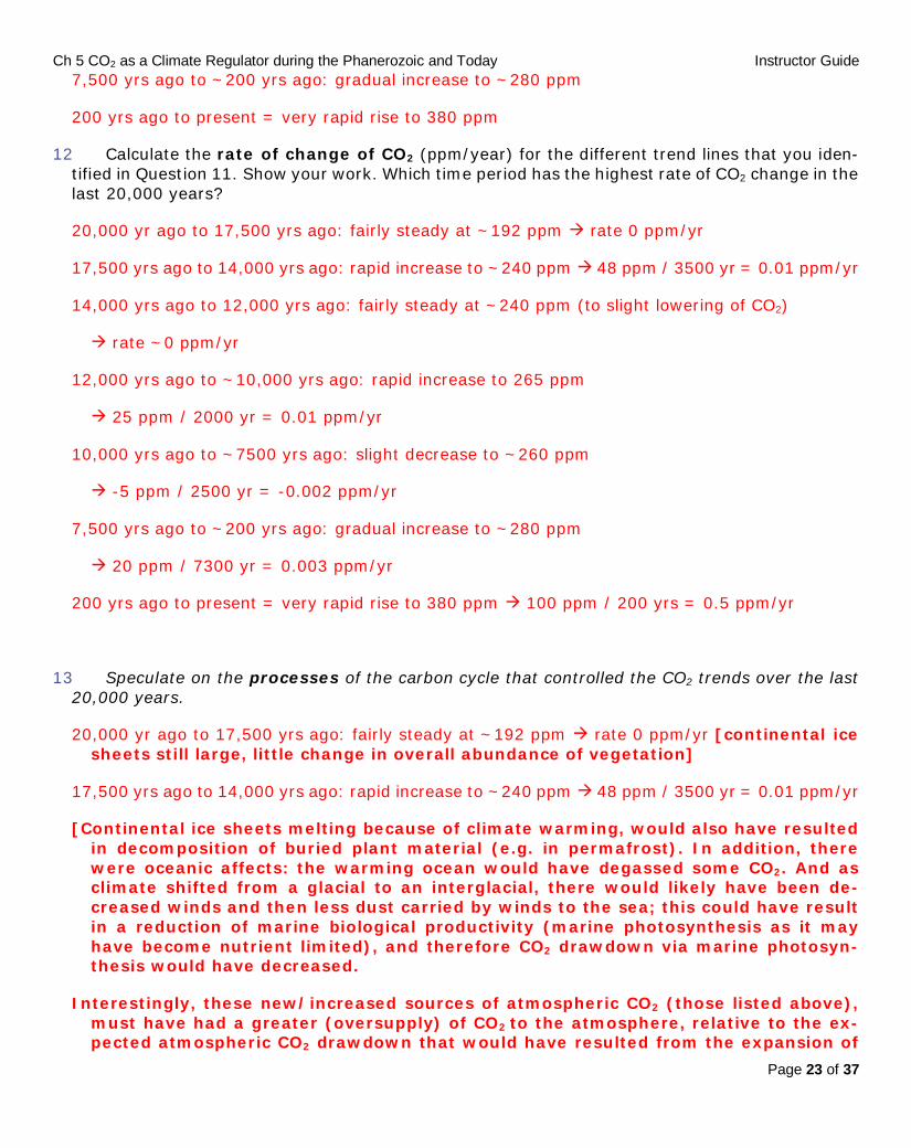
7,500 yrs ago to ~200 yrs ago: gradual increase to ~280 ppm

200 yrs ago to present = very rapid rise to 380 ppm

12 Calculate the rate of change of CO2 (ppm/year) for the different trend lines that you iden-tified in Question 11. Show your work. Which time period has the highest rate of CO2 change in the last 20,000 years?

20,000 yr ago to 17,500 yrs ago: fairly steady at ~192 ppm rate 0 ppm/yr

17,500 yrs ago to 14,000 yrs ago: rapid increase to ~240 ppm 48 ppm / 3500 yr = 0.01 ppm/yr

14,000 yrs ago to 12,000 yrs ago: fairly steady at ~240 ppm (to slight lowering of CO2)

rate ~0 ppm/yr


25 ppm / 2000 yr = 0.01 ppm/yr


-5 ppm / 2500 yr = -0.002 ppm/yr


20 ppm / 7300 yr = 0.003 ppm/yr

200 yrs ago to present = very rapid rise to 380 ppm 100 ppm / 200 yrs = 0.5 ppm/yr

13 Speculate on the processes of the carbon cycle that controlled the CO2 trends over the last 20,000 years.

20,000 yr ago to 17,500 yrs ago: fairly steady at ~192 ppm rate 0 ppm/yr [continental ice sheets still large, little change in overall abundance of vegetation]

17,500 yrs ago to 14,000 yrs ago: rapid increase to ~240 ppm 48 ppm / 3500 yr = 0.01 ppm/yr

[Continental ice sheets melting because of climate warming, would also have resulted in decomposition of buried plant material (e.g. in permafrost). In addition, there were oceanic affects: the warming ocean would have degassed some CO2. And as climate shifted from a glacial to an interglacial, there would likely have been de-creased winds and then less dust carried by winds to the sea; this could have result in a reduction of marine biological productivity (marine photosynthesis as it may have become nutrient limited), and therefore CO2 drawdown via marine photosyn-thesis would have decreased.

Interestingly, these new/increased sources of atmospheric CO2 (those listed above), must have had a greater (oversupply) of CO2 to the atmosphere, relative to the ex-pected atmospheric CO2 drawdown that would have resulted from the expansion of


of 37

land vegetation in areas that were recently deglaciated.]

14,000 yrs ago to 12,000 yrs ago: fairly steady at ~240 ppm (to slight lowering of CO2)

rate ~0 ppm/yr [not much glacial activity (growth or decay)]


25 ppm / 2000 yr = 0.01 ppm/yr

[The final retreat of continental ice sheets because of climate warming, would also have resulted in further decomposition of buried plant material (e.g. in permafrost). In addition, the oceanic affects would have included: a warmer ocean degassing some CO2. And as climate made the final shift from a glacial to an interglacial, there would likely be decreased winds and then less dust carried by winds to the sea; this could have resulted in a reduction of marine biological productivity (marine photo-synthesis, as it may have become nutrient limited), and therefore CO2 drawdown via marine photosynthesis would have decreased.

These new/increased sources of atmospheric CO2 (those listed above), must have had a greater (oversupply) of CO2 to the atmosphere, relative to the expected atmos-pheric CO2 drawdown that would have resulted from the expansion of land vegeta-tion in areas that were recently deglaciated.]


-5 ppm / 2500 yr = -0.002 ppm/yr [slight climatic cooling, decrease in rate of organic decomposition]


20 ppm / 7300 yr = 0.003 ppm/yr [increased warming; continental ice sheets now only in Greenland and Antarctica, greater rate of decomposition]

200 yrs ago to present = very rapid rise to 380 ppm 100 ppm / 200 yrs = 0.5 ppm/yr

[industrialization; burning of fossil fuels]


of 37

Part 5.4. Long-Term Global Carbon Cycle, CO2, and Phanerozoic

Climate History

Long-Term Carbon Cycle As you learned in Part 5.1, carbon reservoirs include the lithosphere, the atmosphere, the ocean, and the biosphere. Carbon is transferred to and from the atmosphere over short time scales (Figure 5.2) and also over long time scales for which plate tectonics and weathering becomes important climatic influences (Figure 5.6).

1 There are over 66,000,000 gigatonnes of carbon stored in the lithosphere (Figure 5.2). What are the long-term processes (Figure 5.6) that transfer this geologically stored carbon to the at-mosphere?

All of the “up” arrows in figure 5.6 are processes that transfer geologically stored carbon to the atmosphere. These include:

• volcanic outgassing (at divergent and convergent plate boundaries; magma contains dissolved gas including CO2),

• weathering of organic carbon (essentially oxidizing

• degassing associated with diagenesis and metamorphism. (As certain minerals are sub-jected to heat and pressure, mineral transformations can take place where water and gases in the mineral structure are driven off. For example:

organic carbon such as peat or coal),

(HEAT)

CaMg(CO3)2 CaCO3 + MgO + CO2 (gas)

(dolomite) (calcite) (periclase) (carbon dioxide)

These processes may require a mini-lecture. Especially why weathering of organic carbon releases CO2, whereas weathering of silicates removes CO2 from the atmosphere (or soil). This concept is explored more in Chapter 10, Section 10.3. Note also that although not pointed out in Figure 5.6, weathering of limestone (CaCO3) can also release CO2 to the atmosphere.

The Berner (1999) GSA Today paper is a good reference on the long-term carbon cycle.


of 37

FIGURE 5.6. Simplified diagram of the long-term carbon cycle. From Berner, 1999. Note that CO2 released at oceanic ridges is considered to be from volcanic sources. Originally drawn by Steve Petsch, University of Massachusetts, Amherst.

2 The rate at which each process transfers carbon from one reservoir to another can change over geologic (i.e., “long”) time scales. Use Figure 5.6 to explain how changing rates of seafloor spreading would affect the rate of CO2 transfer to the atmosphere.

If the rate of sea floor spreading increased then the rate of outgassing at divergent and convergent plate margins would also increase. [The rate of CO2 and CH4 released via diagenesis and meta-morphism would also increase, but countering this would be an increase in the rate of subduction of organic C and carbonate rich-metasediments (CaCO3).]

3 Examine the age distribution map of the seafloor (Figure 5.7). How could the geographic distri-bution of seafloor ages help us determine if seafloor spreading rates have changed in the past?

Distance/Age = Rate of Spreading. While it is a bit of a “back of the envelope calculation”, one can measure the width of the green and the width of the dark red to one side of the ridge (e.g., the North Atlantic is a good place), and calculate the spreading rates. The rate during the Cretaceous (green; from 131-67.7 Ma) was ~2X the rate today (dark red, 9.7-0 Ma).


of 37

FIGURE 5.7. Seafloor age in millions of years. Age determined from the paleomagnetic reversal patterns preserved in ocean crust basalts (see Chapter 3) Map courtesy of NOAA (http://www.ngdc.noaa.gov/mgg/ocean_age/data/2008/image/age_oceanic_lith.jpg).

http://www.ngdc.noaa.gov/mgg/ocean_age/data/2008/image/age_oceanic_lith.jpg�


of 37

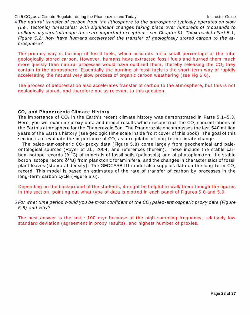
4 The natural transfer of carbon from the lithosphere to the atmosphere typically operates on slow (i.e., tectonic) timescales; with significant changes taking place over hundreds of thousands to millions of years (although there are important exceptions; see Chapter 9). Think back to Part 5.1, Figure 5.2; how have humans accelerated the transfer of geologically stored carbon to the at-mosphere?

The primary way is burning of fossil fuels, which accounts for a small percentage of the total geologically stored carbon. However, humans have extracted fossil fuels and burned them much more quickly than natural processes would have oxidized them, thereby releasing the CO2 they contain to the atmosphere. Essentially the burning of fossil fuels is the short-term way of rapidly accelerating the natural very slow process of organic carbon weathering (see Fig 5.6).

The process of deforestation also accelerates transfer of carbon to the atmosphere, but this is not geologically stored, and therefore not as relevant to this question.

CO2 and Phanerozoic Climate History The importance of CO2 in the Earth’s recent climate history was demonstrated in Parts 5.1–5.3. Here, you will examine proxy data and model results which reconstruct the CO2 concentrations of the Earth’s atmosphere for the Phanerozoic Eon. The Phanerozoic encompasses the last 540 million years of the Earth’s history (see geologic time scale inside front cover of this book). The goal of this section is to evaluate the importance of CO2 as a regulator of long-term climate change.

The paleo-atmospheric CO2 proxy data (Figure 5.8) come largely from geochemical and pale-ontological sources (Royer et al., 2004, and references therein). These include the stable car-bon-isotope records (δ13C) of minerals of fossil soils (paleosols) and of phytoplankton, the stable boron isotope record δ11B) from planktonic foraminifera, and the changes in characteristics of fossil plant leaves (stomatal density). The GEOCARB III model also supplies data on the long-term CO2 record. This model is based on estimates of the rate of transfer of carbon by processes in the long-term carbon cycle (Figure 5.6).

Depending on the background of the students, it might be helpful to walk them though the figures in this section, pointing out what type of data is plotted in each panel of Figures 5.8 and 5.9.

5 For what time period would you be most confident of the CO2 paleo-atmospheric proxy data (Figure 5.8) and why?

The best answer is the last ~100 myr because of the high sampling frequency, relatively low standard deviation (agreement in proxy results), and highest number of proxies.


of 37

FIGURE 5.8. (A) Paleo-atmospheric CO2 proxy and model data for the Phanerozoic Eon; salmon colored area plot shows envelope of modeled CO2 values, including uncertainty; four colored lines represent proxy data; (B) Average value of the combined CO2 proxy data (black line). Standard deviation of the combined data is shown in gray and represents the uncertainty of the data; (C) Frequency distribution of the CO2 proxy data. From Royer et al., 2004.


of 37

6 How do the records from the different independent paleo-atmospheric CO2 proxies compare with the results from the paleo-atmospheric CO2 geochemical model (GEOCARB III; Figure 5.8)?

Very similar for the time periods of overlap, but there are some exceptions (e.g., 150 to 200 Ma).

7 In Part 5.3 (Question 7) you looked up the modern concentration of atmospheric CO2. Draw a horizontal line on Figure 5.8(A) indicating this modern value. Estimate the percentage of the Phanerozoic time (i.e., the last 540 million years) that had a higher CO2 level than today.

Recall that the modern level of atmospheric CO2 is ~392 ppm. Therefore, estimates should be ≥ 90% of the Phanerozoic had a higher CO2 level than today. This is a powerful learning point for students, as most may have previously assumed that modern global CO2 levels (and therefore temperatures) are among the highest of Earth’s history. It’s important that you don’t end the exercise here, or students may erroneously conclude that the recent CO2 trend and related global warming isn’t a big deal CO2 levels (and temperatures) have been higher for most of Earth’s his-tory. The remainder of this exercise explores why the recent changes are a serious concern, even given this geologic context.

Direct evidence for Phanerozoic climate change comes from the rock record. The temporal and spatial distributions of glacial erosion features (e.g., striations on bedrock) and glacial deposits (e.g., end moraines; see Ch. 14 for photos and maps of recent glacial deposits) can be used to constrain the timing and geographic extent of glaciations of the past (Figure 5.9).


of 37

FIGURE 5.9. (A) Paleo-atmospheric CO2 from proxies (black line) and the GEOCARB III model (red line); model uncertainty is represented by the orange shading, (B) time periods of glaciation (dark blue) or cool climates (light blue), and (C) the latitudinal distribution of glaciation. Modified from Royer et al., 2004.

8 Compare the Phanerozoic records of paleo-atmospheric CO2 and glaciation. Is there any correlation between the two records? Describe.

Yes, good correlation: low (<500 ppm) CO2 during periods of long-lived and widespread continental glaciation, and high (>1000 ppm) CO2 during warm periods. However, older glaciations (430 and 520 Ma) do seem to occur when models estimate atmospheric CO2 to have been high. There is little to no CO2 proxy data for the older parts of the record to compare to the model results.


of 37

9 (a) According to the data in Figure 5.9, what is the maximum CO2 level that can support the ex-istence of large ice sheets – those extending past the Arctic and Antarctic circles (66° paleolati-tude)?

Note the strong CO2-temperature relationship for much of the Phanerozoic. Royer et al. (2004) suggest that 500 ppm is a threshold that must be passed (i.e., CO2 must be lower than 500 ppmv) for large ice sheets to exist. It is unlikely that students will have such a refined interpretation, unless they also pay attention to uncertainty (excluding timeslices of high uncertainty, such as those that have no proxy data and only model data in the early Phanerozoic [the late Ordovician glaciation at ~440 Ma]). More likely, student responses will vary widely: 500 ppm or 1000 ppm or 1500 ppm, or even 7000 ppm! Question 9b is important to do as this can lead into a class discussion about data interpretation, and what is robust and what may not be robust data. You may wish to have students read excerpts from the Royer et al. (2004) paper. Other resources to explore are Kump et al. (1999) and Young et al. (2010) – see Supplemental Resources – these explore the seemingly paradoxical late Ordovician glaciation.

(b) Refer back to the sampling frequency and standard deviation data in Figure 5.8. Do you want to modify your answer to question 9a, based on this uncertainty data? How so?

If students were not paying attention to these factors before (question 9a) they hopefully will now. The CO2 level during the glaciations at ~430-440 Ma are highly uncertain, therefore they may lower their glacial threshold CO2 level from several thousand ppm to closer to 1500 or 1000 ppm.

GREENHOUSE AND ICEHOUSE WORLDS Through approximately the last 2 billion years, Earth’s climate has fluctuated – at timescales of tens of millions of years to approximately 100 million years – between relatively cold times, with low atmospheric CO2 levels, long-lived large ice sheets, and low sea levels, and relatively warm times, with high atmospheric CO2 levels, no long-lived large ice sheets, and high sea levels. The warm episodes are described as greenhouse worlds, whereas the cold episodes are described as ice-house worlds.

The occurrence of greenhouse worlds and icehouse worlds in the Earth’s history appears to have been triggered by one or more of several factors: changes in the latitudinal positions of large con-tinents; opening or closing of oceanic gateways, which affect ocean circulation patterns and the movement of heat around the planet; and changes in the global carbon cycle, such as by the uplift and chemical weathering of mountain ranges (see Chapter 10 on the Oi1 event), by changes in the rates of seafloor spreading or other volcanic activity, or by changes in biological cycling of carbon.

10 Read the box above. Was the Cretaceous Period (145.5 Ma to 65.5 ma) a greenhouse world or an icehouse world?

Greenhouse world

11 Do we currently live during a greenhouse world or an icehouse world?

Icehouse world (this is usually a surprise to students).

12 How can you reconcile your answer to Question 11 with the documented global warming that is occurring today (e.g., Part 5.3)?


of 37

This is question of scale: we are in an icehouse world, but one that is warming. Other students may be more specific if they know about glacial and interglacial periods (which are only relevant terms during Icehouse times). We are in an interglacial of the current Icehouse, and climate should have already begun to cool towards the next glacial period, according to Milankovitch theory. However, conditions have not begun to cool because the natural processes have been outweighed by hu-man-induced changes. This is explored more in Chapter 8, Part 8.3.

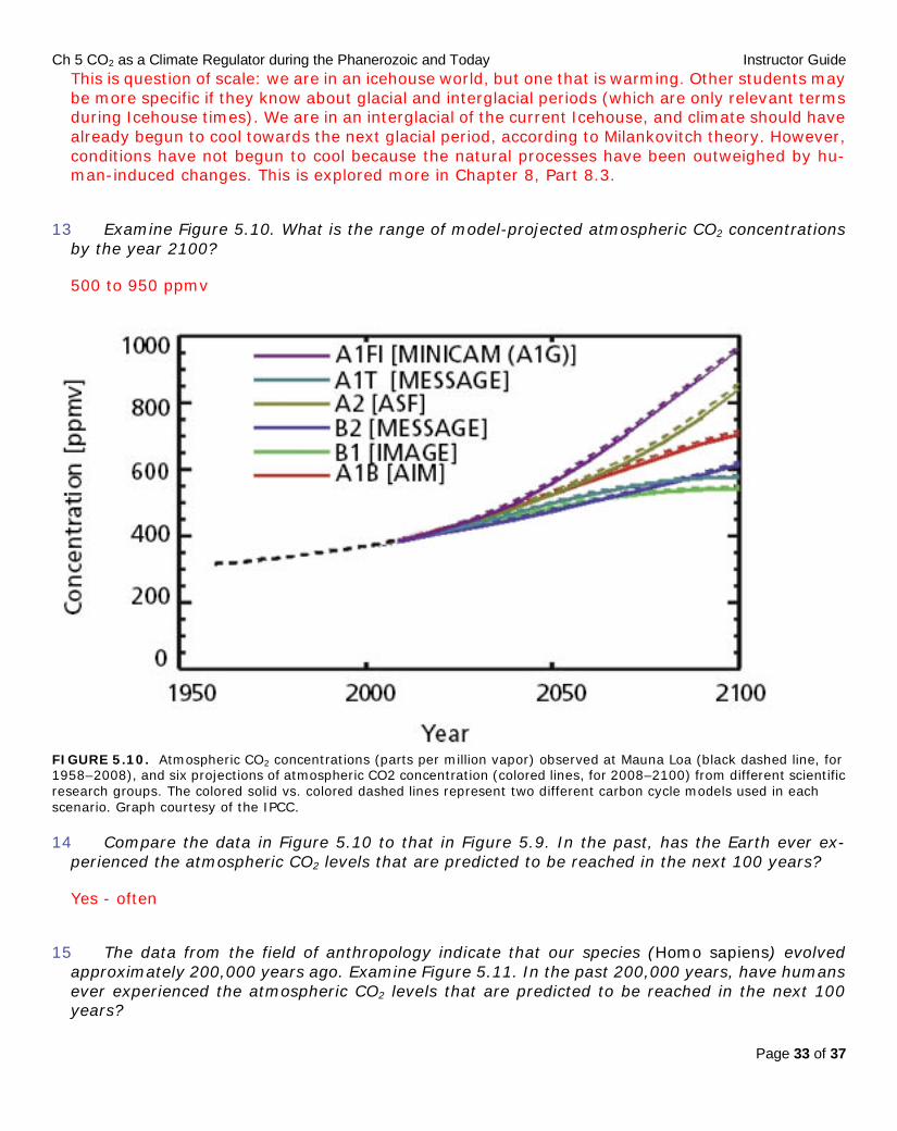
13 Examine Figure 5.10. What is the range of model-projected atmospheric CO2 concentrations by the year 2100?

500 to 950 ppmv

FIGURE 5.10. Atmospheric CO2 concentrations (parts per million vapor) observed at Mauna Loa (black dashed line, for 1958–2008), and six projections of atmospheric CO2 concentration (colored lines, for 2008–2100) from different scientific research groups. The colored solid vs. colored dashed lines represent two different carbon cycle models used in each scenario. Graph courtesy of the IPCC.

14 Compare the data in Figure 5.10 to that in Figure 5.9. In the past, has the Earth ever ex-perienced the atmospheric CO2 levels that are predicted to be reached in the next 100 years?

Yes - often

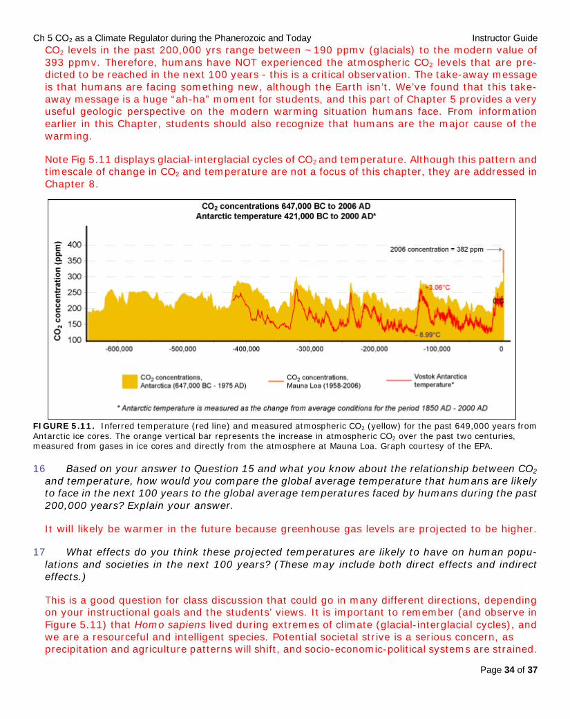
15 The data from the field of anthropology indicate that our species (Homo sapiens) evolved approximately 200,000 years ago. Examine Figure 5.11. In the past 200,000 years, have humans ever experienced the atmospheric CO2 levels that are predicted to be reached in the next 100 years?


of 37

CO2 levels in the past 200,000 yrs range between ~190 ppmv (glacials) to the modern value of 393 ppmv. Therefore, humans have NOT experienced the atmospheric CO2 levels that are pre-dicted to be reached in the next 100 years - this is a critical observation. The take-away message is that humans are facing something new, although the Earth isn’t. We’ve found that this take- away message is a huge “ah-ha” moment for students, and this part of Chapter 5 provides a very useful geologic perspective on the modern warming situation humans face. From information earlier in this Chapter, students should also recognize that humans are the major cause of the warming.

Note Fig 5.11 displays glacial-interglacial cycles of CO2 and temperature. Although this pattern and timescale of change in CO2 and temperature are not a focus of this chapter, they are addressed in Chapter 8.

FIGURE 5.11. Inferred temperature (red line) and measured atmospheric CO2 (yellow) for the past 649,000 years from Antarctic ice cores. The orange vertical bar represents the increase in atmospheric CO2 over the past two centuries, measured from gases in ice cores and directly from the atmosphere at Mauna Loa. Graph courtesy of the EPA.

16 Based on your answer to Question 15 and what you know about the relationship between CO2 and temperature, how would you compare the global average temperature that humans are likely to face in the next 100 years to the global average temperatures faced by humans during the past 200,000 years? Explain your answer.

It will likely be warmer in the future because greenhouse gas levels are projected to be higher.

17 What effects do you think these projected temperatures are likely to have on human popu-lations and societies in the next 100 years? (These may include both direct effects and indirect effects.)

This is a good question for class discussion that could go in many different directions, depending on your instructional goals and the students’ views. It is important to remember (and observe in Figure 5.11) that Homo sapiens lived during extremes of climate (glacial-interglacial cycles), and we are a resourceful and intelligent species. Potential societal strive is a serious concern, as precipitation and agriculture patterns will shift, and socio-economic-political systems are strained.

http://www.epa.gov/climatechange/science/pastcc.html�


of 37

III. Summative Assessment

There are several ways the instructor can assess student learning after completion of this exercise. For example, students should be able to answer the following questions after completing this ex-ercise (note this is just a small sampling of the types of questions that could be asked): 1. Is the modern climate one of a Greenhouse World or an Icehouse World?

a. Greenhouse World b. Icehouse World

2. True or False: Atmospheric CO2 concentrations are predicted to rise by the year 2100 to a level never before experienced by humans.

a. true b. false

3. True or False: Atmospheric CO2 concentrations are predicted to rise by the year 2100 to a level never before experienced by Earth.

a. true b. false

4. Based on CO2 proxy data and models, what percent of Phanerozoic time (i.e., the last 600 million years) had a higher atmospheric CO2 concentration than today? a. 0%

b. 0.5% c. ~25% d. ~75% e. >90%

5. Which of the following is closest to the atmospheric CO2 level today? a. 280 ppm b. 392 ppm c. 560 ppm d. 1508 ppm e. 5000 ppm

6. How many Icehouse Worlds have existed over the last 500 million years?

a. 10 b. 5 c. 3 d. 1

7. The Earth’s greenhouse effect a. Keeps Earth’s average temperature within a range such that liquid water can exist at the

Earth’s surface b. Absorbs incoming solar radiation c. Absorbs outgoing infrared radiation d. All of the above e. A and C only


of 37

8. Positive internal Earth system feedbacks a. Always amplify climate changes initially caused by external forcing. b. Always cause climate warming c. Help maintain a constant climate d. Both A and B

9. The Radiative Forcing (RF) of CO2

a. Is calculated by taking the square root of the change in CO2 concentration (ppm) and multiplying by a constant.

b. Is a measure of the direct influence that atmospheric CO2 levels have on altering the balance of incoming and outgoing energy in the Earth-atmosphere system.

c. Takes into account climate system feedbacks that involve CO2. d. All of the above e. A and C only

10. True or false: on average, an atom of carbon spends more time in soil than in the atmosphere. a. True b. False

11. What is the largest reservoir of carbon in the Earth system?

a. The atmosphere b. The lithosphere c. The surface ocean d. Soil e. The terrestrial biosphere

12. Short answer: Compare and contrast the short and long-term carbon cycles. 13. Short answer: Compare and contrast the concepts of “radiative forcing” and “climate system feedbacks”. 14. Short answer: Compare and contrast icehouse and greenhouse worlds. Which of these climate states dominated much of the Phanerozoic? Which of these states is the Earth currently in? 15. How do changes in land use affect (a) albedo, (b) atmospheric CO2, and (c) temperature? IV. Supplemental Materials

• For an engaging overview of Phanerozoic climate watch the AGU 2009 Bjerknes Lecture video (~ 50 minutes) by Dr. Richard Alley, The Biggest Control Knob: Carbon Dioxide in Earth's Climate History http://www.agu.org/meetings/fm09/lectures/videos.php

• This chapter focused on several key papers that examine Phanerozoic CO2 and carbon cycling. In particular follow-up discussions could focus on critical reading of the following (full citation given in the Reference section below):

o Berner (1999) for a discussion of the long term carbon cycle o Joos and Spahni (2008) for a comparison of natural and anthropogenic radiative forcing o Royer (2004) for a reconstruction of Phanerozoic CO2 based on model and proxy data.

A good follow-up to this 2004 paper is: Royer, D.L. (2006). CO2-forced climate thresholds during the Phanerozoic, Geochimica et Cosmochimica Acta, 70, 5665-5675.

http://www.agu.org/meetings/fm09/lectures/videos.php�


of 37

• The Intergovernmental Panel on Climate Change (IPCC) has numerous references online (http://www.ipcc.ch/) for scientists and non-scientists. The 2007 Synthesis Report Summary for Policymakers is a good place to begin: http://www.ipcc.ch/publications_and_data/ar4/syr/en/spm.html

• The Encyclopedia of Earth has a wide variety of online resources on modern climate change (causes, consequence): http://www.eoearth.org/climatechange and http://www.eoearth.org/article/Site_Map_for_the_Climate_Change_Collection?topic=49491 For example,

o A synopsis of NOAA data that finds 2011 is the 9th warmest year on record (since 1880); http://www.eoearth.org/news/view/172896/?topic=49491.

o A synopsis of NIH research on the health effects of climate change; http://www.eoearth.org/news/view/170725/?topic=49491.

o A definition of radiative forcing, http://www.eoearth.org/article/Radiative_forcing. • Monthly updates of atmospheric CO2 concentrations measured at Mauna Loa Observatory,

Hawaii, can be found at: www.esrl.noaa.gov/gmd/ccgg/trends/ • In Part 5.4 the early Phanerozoic glaciation (~440 Ma) is puzzling because it doesn’t seem to

match model results of high CO2. This puzzle is directly addressed in the following two papers: o Kump, L.R., Arthur, M.A., Patzkowsky, M.E., Gibbs, M.T., Pinkus, D.S., and Sheehan,

P.M., (1999). A weathering hypothesis for glaciations at high atmospheric pCO2 during the Late Ordovician, Palaeography, Palaeoclimatology, Palaeoecology, 152, 173-187.

o Young, S.A., Saltzman, M.R., Ausich, W.I., Desrochers, A., and Kaljo, D., (2010). Did changes in atmospheric CO2 coincide with latest Ordovician glacial-interglacial cycles?, Palaeography, Palaeoclimatology, Palaeoecology, 296, Issue 3-4, 376-388.

• This exercise focused on carbon dioxide (CO2) during the Phanerozoic. For an analysis of methane (CH4) during the Phanerozoic see: Bartdorff, O., Wallmann, K., Latif, M., and Se-menov (2008), Phanerozoic evolution of atmospheric methane, Global Biogeochemical Cycles, 22, GB1008, doi:10.1029/2007GB00298.

V. References

Berner, R.A., 1999, A new look at the long-term carbon cycle. GSA Today, 9, 2–6.

Forster, P., et al., 2007, Changes in atmospheric constituents and in radiative forcing. In Climate Change 2007: The Physical Science Basis. Contribution of Working Group I to the Fourth As-sessment Report of the Intergovernmental Panel on Climate Change, Solomon, S., et al. (eds), Cambridge University Press, Cambridge, UK.

Joos, F. and Spahni, R., 2008. Rates of change in natural and anthropogenic radiative forcing over the past 20,000 years. Proceedings of the National Academy of Sciences of the USA, 105 (5), 1425–30, http://www.pnas.org/content/105/5/1425.full.

Kiehl, J. T. and Trenberth K.E., 1997, Earth’s annual global mean energy budget. Bulletin of the American Meteorological Society, 78 (2), 197–208.

Rahmstorf, S., 2008, Anthropogenic climate change: revisiting the facts. In Global Warming: Looking Beyond Kyoto, Zedillo, E. (ed), Brookings Institution Press, Washington DC, and Yale Center for the Study of Globalization, Newhaven, Connecticut, pp. 34–53. http://www.pik-potsdam.de/∼stefan/Publications/Book_chapters/Rahmstorf_Zedillo_2008.pdf.

Royer, D.L., et al., 2004, CO2 as a primary driver of Phanerozoic climate. GSA Today, 14, 4–10.

Ruddiman, W. F., 2008, Earth’s Climate Past and Future, W.H. Freeman and Co., New York, 388 pp.

http://www.ipcc.ch/�

http://www.ipcc.ch/publications_and_data/ar4/syr/en/spm.html�

http://www.eoearth.org/climatechange�

http://www.eoearth.org/article/Site_Map_for_the_Climate_Change_Collection?topic=49491�

http://www.eoearth.org/article/Site_Map_for_the_Climate_Change_Collection?topic=49491�

http://www.eoearth.org/news/view/172896/?topic=49491�

http://www.eoearth.org/news/view/170725/?topic=49491�

http://www.eoearth.org/article/Radiative_forcing�

http://www.esrl.noaa.gov/gmd/ccgg/trends/�

Instructor Guide Chapter 5 CO2 as a Climate Regulator ... · Chapter 5CO 2 as a Climate ... and...

Documents

Transcript of Instructor Guide Chapter 5 CO2 as a Climate Regulator ... · Chapter 5CO 2 as a Climate ... and...