DTI

0

EECTE

DEVELOPMENT OF AN AUTOMATIC GROUNDCOLLISION AVOIDANCE SYSTEM

USING A DIGITAL TERRAIN DATABASE

THESIS

Gregory W. BiceCaptain, USAF

A•flT/GAE/ENY/89D-03

II

DEPARTMENT OF THE AIR FORCE

AIR UNIVERSITY

AIR FORCE INSTITUTE OF TECHNOLOGY

Wright-Patterson Air Force Base, OhioI DISTORBUTION STATEMMIT A

Apj'rovod fo'r pubUi • eIaa 89 12 29 035Digiribudzn U ,Um•led

AFIT/GAE/ENY/89D-03

DEVELOPMENT OF AN AUTOMATIC GROUNDCOLLISION AVOIDANCE SYSTEM

USING A DIGITAL TERRAIN DATABASE

THESIS

Gregory W. BiceCaptain, USAF

AFIT/GAE/ENY/89D-03

Approved for public release; distribution unlimited

DTIC

" ELECTF

SJAN 0 2 19901

III

!

IAFIT/GAE/ENY/g9D-03

I

DEVELOPMENT OF AN AUTOMATED GROUND

fl COLLISION AVOIDANCE

SYSTEM USING A DIGITAL TERRAIN DATABASE

THESIS

Presented to the Faculty of the School of Engineering

of the Air Force Institute of Technology

* Air University

In Partial Fulfillment of the

Requirements for the Degree of

Master of Science in Aeronautical Engineering

I

Gregory W. Bice, B.S.

Captain, USAF

December 1989

Approved for public release; distribution unlimited

I

I

I

I The purpose of this study was to develop a working control system that

would perform automatic ground collision avoidance using a digital terrain data-

base. A secondary purpose was to show the potential of the digital terrain data-

base for improving the mission capabilities of combat aircraft. Both of those

purposes were fulfilled in this thesis.

The topic studied in this thesis has current applications to the Air Force,

3 therefore, I feel work should continue to be devoted to this area of research.

Potential savings in both aircraft and pilots make automated ground collison

avoidance a worthwhile endeavor.

In developing and writing this thesis, my thanks and appreciation go to

i many people who have made the rough road a little smoother. I am very thank-

ful for the engineering prowess and persistance of my thesis advisor, Capt Curt

Mracek. His understanding and assistance made the hard times in this thesis a

3 little easier. Thanks also go to Capt Brett Ridgely for his assistance in control

system analysis. I also wish to extend a hand of appreciation to my sponsor Mr.

I Finley Barfield of the Flight Dynamics Laboratory for the use of facilities, as-

sistance in deciphering control law diagrams, and his expert knowledge of the

F-16. Under the area of morale, I wish to thank all of my friends in the Bullpen

for their humor and support. I will miss the gatherings of the "Friday at the

Flywright" gang who helped make AFIT a bearable place. Finally, I am eternal-

I ly thankful for the support of my wife, Susan, who put up with my late nights, n For

bad days, and gave me a wonderful daughter, Lauren. Thanks Lord.

Gregory W. Bice .ed 0

DJO~.rbtton/

I'" CrED AvaUbl.illty Codes

ii "-- .at a/orI

i ii

II

Table of Contents

Page

Preface ii

List of Figures ..... .... .... ................. . v

I List of Tables ..................................... viii

Abstract ........................................ ix

I. Introduction ......... .............................. 1-1

Background ........ ........................... 1-1

Current GCAS Limitations ...................... 1-2Digital Terrain Database ...... ................. 1-3

Problem Statement ............................... 1-3

II. State-Space Model Development ......................... 2-1

Methodology ........ ........................... 2-1Matrix Development .............................. 2-2

LogtdnlAxs...........................2-5SLongitudinal Axis................. ..... 2-

Closed Loop System Derivation ................... 2-10Lateral-Directional Axis ........................ 2-14

State-Space Verification Using Sequential Loop Closure . . . 2-23

III. Terrain Avoidance Control System Development ........... 3-1Terrain Avoidance Equation Derivation ............. ..... 3-1Control System Design Process ...................... 3-4Controller State-Space Derivation ..................... 3-13Terrain Model and Evaluation Plan .................... 3-15

IV. Results and Discussion ............................... 4-1Altitude Controller Evaluation ...................... 4-1Alternate Terrain Avoidance Approach and Evaluation . . . 4-11

V. Conclusions ........ .............................. 5-1

VI. Recommendations .................................. 6-1

Appendix A: F-16 Control Derivatives and Trim Conditions ........ A-)

I iii

I

Page

Appendix B: F-16 Layout, Angular Definitions, andSign Conventions ...... ..................... B-1

Appendix C: Control Derivative Conversion Program ......... ..... C-1

Appendix D: Development of Linearized Equations of Motion . ... D-1

Appendix E: State-Space Control System Matrix ............ ..... E- 1

Appendix F: Altitude Controller Root Locus Plots ........... ..... F-I

Bibliography ....................................... Bib-I

Vita ............................................ V-1

iv

List ofF~igures

Figure Page

2.1. Modified F-16 Longitudinal Control System ............. 2-3

2.2. F-16 Lateral-Directional Control System .................... 2-4

2.3. Open Loop Longitudinal State-Space System ..... ............ 2-8

2.4. Feedback Matrix in the Laplace Domain .................... 2-9

2.5. General Closed Loop State-Space System ..... .............. 2-12

2.6. Aircraft Longitudinal State Responses To Step Pitch RateCommand Input: (a) Pitch Rate, (b) Normal Load Factor,

(c) Angle of Attack, (d) Altitude ...... ................... 2-15

2.7. Aircraft Lateral-Directional State Responses to Step Roll RateCommand Input: (a) Bank Angle, (b) Roll Rate, (c) Yaw Rate,

(d) Lateral Acceleration ....... ........................ 2-19

I 2.8. Lateral-Directional Control Surface Response to aStep Roll Rate Input: (a) Flaperon, (b) Rudder ..... ........... 2-20

3 2.9. Roll Rate Response Comparisons Between the F-16 and A-4D . . . 2-22

2.10. Aircraft Lateral-Directional State Responses Given Initial BankAngle Condition of 180 degrees: (a) Bank Angle, (b) Roll Rate,(c) Yaw Rate, (d) Lateral Acceleration ...................... 2-24

2.11. Control Surface Response for 180 degree Initial Conditions:(a) Flaperon, (b) Rudder .............................. 2-25

2.12. F-16 Longitudinal Control System Displayed in Loop Form . . .. 2-26

3.1. Scheme for Implementing Terrain Avoidance .................. 3-2

I 3.2. Terrain Avoidance Control System Diagram. .................. 3-5

3.3. Terrain Avoidance Control System In Loop Form ..... .......... 3-6

1 3.4. Aircraft Pitch Rate Response to Step Pitch RateCommand Input ........ ............................ 3-8

3.5. Aircraft Flight Path Angle Response to Step FlightPath Angle Command Input ...... ...................... 3-10

I 3.6. Aircraft Altitude Response to Step Altitude Command Input ..... .. 3-12

I v

I!___

IFigure Page

3.7. Terrain Obstacle Model .............................. 3-15

3.8. Enlarged View of Simulated Terrain Showing the Conceptof a 300-foot Look-Ahead Distance ....................... 3-16

4.1. Altitude Response vs Terrain for 0-foot Look-Ahead Distance ... 4-2

4.2. Altitude Response vs Terrain for 100-foot Look-Ahead Distance . . . 4-3

_ 4.3. Altitude Response vs Terrain for 300-foot Look-Ahead Distance . 4-5

4.4. Altitude Response vs Terrain for 600-foot Look-Ahead Distance . . . 4-6

4.5. Altitude Response vs Terrain for 1200-foot Look-Ahead Distance . . . 4-8

4.6. Altitude vs Range for 1200-foot Look-Ahead Distance ......... .. 4-9

4.7. Altitude Response With Reduced Gain in Flight Path Loop for1200-foot Look-Ahead Distance ......................... 4-10

4.8. Aircraft Pitch Rate and Load Factor Response for 1200-footLook-Ahead Distance: (a) Altitude vs Terrain, (b) Pitch Rate3 and Load Factor Response ............................. 4-12

4.9. Horizontal Tail Response for Terrain Avoidance Maneuver

3 With 1200-foot Look Ahead Distance ...................... 4-13

4.10. Altitude Error vs Range for Various Look-Ahead Distances ...... .4-14

3 4.11. Alternate Method for Implementing Terrain Avoidance .......... 4-15

4.12. Aircraft Response Using Modified Approach for 300 foot3 Look-Ahead Distance ................................ 4-17

4.13. Altitude Error Comparison Between Different TerrainAvoidance Implementations ............................ 4-18

4.14. Aircraft Pitch Rate and Load Factor Response forModified Terrain Avoidance Approach ..................... 4-19

1 4.15. Horizontal Tail Response for Modified TerrainAvoidance Approach ................................ 4-20

3 6.1. Time History of F-16 Terrain AvoidanceUsing 'Bang-Bang' Inputs .............................. 6-4

1 6.2. Aircraft Altitude vs Range Using 'Bang-Bang' Inputs .......... 6-5

6.3. Aircraft State Responses for Terrain AvoidanceWith 'Bang-Bang' Inputs: (a) Pitch Rate, (g) Incremental GAngle of Attack (d) Pitch Angle .......................... 6-6

I vi

I___

IFigure Page1 6.4. Aircraft Pitch Rate Response vs Pitch Rate Command

for 'Bang-Bang' Inputs ........ ........................ 6-7

I B. 1. F-16 Layout and General Arrangement ...... ................ B-2

B.2. F-16 Axis Systems and Sign Conventions .................... B-3

F. 1. Root Locus of Flight Path Angle to Pitch RateCommand Without Compensation ...... ................... F-3

I F.2. Root Locus of Flight Path Angle to Flight Path AngleCommand With Compensation ............................ F-4

F.3. Expanded View of Root Locus in Figure F.2 ................... F-5

F.4. Root Locus of Altitude to Flight Path Angle CommandWithout Compensation ....... .......................... F-6

F.5. Expanded View of Root Locus in Figure F.4 .... .............. F-7

I F.6. Root Locus of Altitude to Flight Path Angle CommandWith Compensation ................................... F-8

F.7. Expanded View of Root Locus in Figure F.6 ................... F-9

F.8. Root Locus of Altiiude to Altitude Command5 Transfer Function ................................... F-10

IIIIIIII vii

I_ _ _ _ _ _ _ _ _ _ _ _ _ _ _ __ _ _ _ _ _ _ _ _

Listof__Tak.

Table Page

2.1. Selected Trim Conditions fo Linearized Model .............. .... 2-2

2.2. Eigenvalues and Representative Modes of theF-16 Longitudinal Axis .................................. 2-7

2.3. F- 16 Longitudinal Closed Loop Poles ........................ 2-14

2.4. Eigenvalues of Lateral-Directional Axis ....................... 2-17

I

I

IIIvi

I

During the past several years, the Air Force has experienced an increasing number

of single seat aircraft mishaps due to what is termed 'controlled flight into terrain'. To

combat this phenomenon, several ground collision avoidance systems (GCAS) have

been developed to warn the pilot of a potential collision with the terrain if some action

is not taken. However, all current systems have shortcomings pertaining to the sensors

that are used and the recovery maneuver that is flown. The USAF is evaluating the

potential of digital terrain databases for onboard navigation and terrain avoidance in

combat aircraft. The purpose of this thesis was to develop a control system for per-

I forming terrain avoidance using a simulated terrain database. This study was conduc-

ted for an F-16 aircraft in level flight at 0.6 Mach and sea level conditions. A state

space model of the aircraft and its flight control system was developed using aircraft

control derivatives, an F- 16 control law diagram, and traditional linearization techni-

ques on the aircraft equations of motiot. A control system for implementing terrain

3 avoidance was derived based on the look-ahead capability of the terrain database. Con-

trol system response was evaluated using a simulated terrain obstacle and various look-

ahead distances on the terrain database. Results indicated that a 1200 foot or roughly

3 1.8 second look-ahead distance provided good improvement in terrain avoidance

capabilities for the F-16 compared to looking strictly downward from the aircraft for

3 terrain information.

IIU

I

DEVELOPMENT OF AN AUTOMATED GROUNDCOLLISION AVOIDANCE SYSTEM USING

A DIGITAL TERRAIN DATABASE

During the past four to five years, the Air Force has recognized that an increasing

number of accidents in fighter and attack aircraft, such as the F-16 and A-10, have been

due to a phenomenon called 'controlled flight into terrain', or CFIT. These are acci-

dents in which good aircraft, flown by capable pilots, crash into the terrain due to pilot

incapacitation, disorientation, or distraction. Aggressive maneuvers performed at low

altitude, such as breaking off of the target after weapon release, can cause g-induced

loss of consciousness GLOC) and spatial disorientation; the latter happening more at

night or in clouds where reference points can become lost. The rise in the number cf

CFIT accidents can in part be attributed to the increased emphasis that has been placed

on the close air support / battlefield air interdiction (CASfBAI) role.

To combat the problems presented by CFIT, several systems have been developed

to help in preventing CFIT accidents. These systems, called ground collision avoid-

ance systems (CGAS) or ground proximity war'ning systems (GPWS), monitor aircraft

states such as altitude above ground level (AGL), airspeed, and attitude. This informa-

tion is in turn fed to a computer algorithm which calculates a pull-up initiation altitude

that will allow the aircraft to avoid impacting the terrain or penetrating a pre-deter-

mined buffer altitude. Whenever the pull-up altitude is equal to or less than the actual

3 AGL altitude of the aircraft, a warning is sent to the pilot that he must initiate a pre-

scribed pull-up maneuver. One system, developed for use on the Advanced Fighter

I'

ITechnology Integration (AFrl)/F-16, performed the pull-up maneuver automatically by

rolling to a wings-level attitude and performing a 5-g pull-up (1:21). This automated

I capability, while having several advantages over the previously described manual

GCAS systems, has not been put into operational use due to computer and autopilot

limitations.

Current GCAS Limitations. While these GCAS implementations have worked to

varying degrees by saving pilots and aircraft, they have limitations. First is the issue

of manual versus automiated recovery. A manual GCAS must incorporate an allowance

for pilot reaction time into its pull-up calculations, and, since reaction times vary from

pilot to pilot, the pull-up maneuver will not be identical. Furthermore, this type of

IGCAS relies solely on the pilot to recover the aircraft once a pull-up warning is given;

pilot incapacitation breaks the recovery system loop. The automated GCAS recovery

maneuver has the capability to be highly repeatable and consistent because it is not

reliant on the pilot, hence, the allowance for pilot reaction time is not necessary. The

I disadvantages of an automated GCAS are the computer limitations of current aircraft

and pilot distrust of automated recovery systems (1:41). Reference 1 examines the is-

sue of pilot-vehicle interface in greater detail.

The second limitation in all current GCAS schemes lies in the sensors that feed

terrain information into the collision avoidance algorithm. Radar altimeters are cur-

I rently used to provide this data, however, they essentially look dowrw:.rd from the air-

craft and have limited look-ahead capability. This is a major drnwback when traversing

over rough to semi-rough terrain which tends to render a GCAS ,iseless. Aircraft pos-

sessing forward-looking radars, such as the B- lB and the F-I 11, implement terrain fol-

lowing systems which are related to ground collision avoidance systems in a broad

sense; the difference being a GCAS should operate as a backup system while the pilot

or autopilot is flying the aircraft. Most fighter and attack aircraft do not possess large

I 1-2I_ _ _ _ _ _ _ __ _ _ _ _ _ _ _

IIforward-looking radars and must rely on a radar altimeter for terrain information, how-

ever, advances in the area of digital terrain databases may solve this problem.

I Digital Terrain Database. The digital terrain database (DTD) has the capability to

store large areas of terrain in compact form such as a cassette tape and uses an inertial

navigation unit to update aircraft location. Using a DTD will give onboard systems the

I ability to analyze terrain 360 degrees around the aircraft, eliminate the requirement for

a forward sensor, and greatly enhance covert capabilities. With the DTD, future GCAS

systems will be able to perform 'smarter' pull-up recovery maneuvers by having the

capability to maneuver over and around the terrain obstacle, not merely pulling up to

avoid it (1:39-41). This will provide the pilot with a safety system that will not degrade

I mission performance. The question that must be addressed then is how the terrain

avoidance system should be implemented and what should it accomplish aside from

avoidirg the terrain.

*Problem Statement

This study will attempt to derive a recovery maneuver based on the capabilities of

the digital terrain database to 'see' terrain ahead of the aircraft. The idea behind this

approach to the terrain avoidance problem is to provide the aircraft with maneuvering

capabilities so that it can continue on a pre-planned mission course while also avoiding

I threatening terrain. Because of the importance of being at a specified set of conditions

during ingress to the target area, the terrain avoidance system should also return the

aircraft to its initial conditions before the recovery maneuver was initiated. All solu-

tions and results will be predicated on the assumption of perfect terrain data correlation

I and registration. A linear state-space representation of the aircraft and control system

i will be constructed so that computer programs such as MATRIXx can be used to ana-

lyze aircraft responses (Reference 7). Inputs consisting of pitch rate and roll rate will

I be made to the control system through the autopilot control paths. The theory for the

I 1-3

I

basis of the recovery maneuver will be derived, and terrain avoidance capabilities will

be evaluated for several different look-ahead distances on the DTD. Finally, the results

of this study will be examined and conclusions drawn as to what the minimum required

look-ahead distance might be. Recommendations will be made for further study and

development of the terrain avoidance problem.

IIIII

III

I 1-4

I i_ _l IiI_ _II

U II.ModeleDevelModen

Ihl g.

In order to facilitate the development of a ground coilision avoidance system, a

state space model of the F-16 was created. Research showed that a model for the

design conditions of M = 0.6 and sea level altitude did not exist, and, therefore, one had

to be developed using the control derivatives for the F-16. The trim condidons and

control derivatives for this condition are detailed in Appendix A. Appendix B contains

a layout of the F-16 along with angular definitions, and sign conventions for control

surface deflections.

In order to construct a state-space representation of any control system, a

condition must be selected about which to linearize the equations of motion. The

control law diagram, which is not shown, was linearized about the conditions of M =

0.6 and an altitude of sea level. No pilot inputs were used, and therefore, all paths

associated with pilot inputs can be ignored, as can all trim inputs. Furthermore, since

the horizontal tail is normally used to command both pitch and roll rates, an effective

aileron/flaperon input was created so that the longitudinal axis motions could be

decoupled from those of the lateral-directional axis. This effective aileron deflection

was defined to be the flaperon deflection plus one-fourth of the horizontal tail deflec-

tion:

8Feff = SF + .25 8HT (2.1)where:

8 Fff = effective flaperon deflection (deg)

S= flaperon deflection (deg)

8 HT = horizontal tail deflection (deg)

2-1

This effective flaperon deflection was used only for roll rate commands; there was no

aileron deflection when the horizontal tail was used to command normal load factor.

The values of the control derivatives were also adjusted using the same formula as Eq

(2.1).

The only other modification made to the control law diagram was changing the

longitudinal autopilot from commanding load factor to commanding pitch rate. This

involved adding several gains to convert the commanded pitch rate to normal load

factor using the steady-state Z-axis acceleration equation:

An = qU0 / [ (57.3)(32.2)] (2.2)Iwhere,An = normal acceleration at pilot station (g)

q = pitch rate (deg/s)

U. = steady-state forward velocity (fit/s)

Figures 2.1 and 2.2 show the final configuration of the linearized F- 16 control

laws which are separated into the longitudinal axis and lateral-directional axis respec-

tively. The control laws have been put into a momv conventional form to aid in visual-

izing the feedback paths.

Matrix Development

A state-space system was use to facilitate analysis of aircraft response. This

involved selecting a Mach number and altitude about which the equations of motion

would be linearized. The selected conditions are listed in Table 2.1.

Table 2.1: Selected Trim Conditions for Linearized Model

Mach= 0.6 Altitude = sea level

True Airspeed (VT) = 670 ft/s Pressure (Pa) = 2116.216 lb/ft2

Impact Pressure (qc) = 583 lb/ft2 (qcPa) = 0.2755

2-2

-s + 601 (57.3)(32.2)

IA

ýHT,.,

+ Gain 0,_+ E_+ _20 rA A,

F3 a

I Figure 2.1- Modified F-16 Longitudinal Control Sistemn

I2-

II 2-10

I

I I I

IIIII , +

cmd so 2 0 A PS+5 i s20

r Ay1 Cr

6,R"m 1 20 I a p so

II r -- w

++5

3+ .027A.R.I.

Figure 2.2: F-16 Lateral-Direction&l Control System

I1I

I

I3 It is important to note that impact pressure, qc, is not the same as dynamic pressure,

q = (0.5)pV2 . The reason for noting this is that the scheduled gains for the control sys-

tern are based on impact pressure and not dynamic pressure. There were several rea-

sons for selecting the listed conditions, first being the fact that this is situated well

within the envelope of the F-16. A second reason was that by selecting sea level

I conditions, any potential mistakes with pressure and density ratios are avoided since

these ratios are normally used to calculate true airspeed, static pressure, and impact

3 pressure at altitude. The final rationale for selecting these conditions was the

requirement for a 5-g load factor capability without incurring very high angles-of-attack

I which would violate the small angle approximations made during the linearization

3 process.

Data on the control derivatives were obtained from the Flight Dynamics

3 Laboratory (WRDC/FIGX) for the stated conditions. Values for the control derivatives

were given in the stability axis, and a computer program, listed ira Appendix C, was

I used to convert these values to the aircraft body axis (8:276). Appendix D details the

development of the equations of motion and the control derivatives and their placement

in the state-space matrix (8:236). The equations of motion were developed using per-

3 turbation techniques and ignoring all terms that were second order and higher. For

purposes of convenience, the system state-space matrix was broken down into the

3 longitudinal and lateral-directional axes to aid in forming the closed loop system. This

could be done since these two axes were decoupled from each other. The closed loop

I derivation of each axis will now be addressed separately.

I Longitudinal Axis. The states used in building the longitudinal state-space system

wereI= [u a 0 q BHT h.,i JT

3 2-5

I

where

u = incremental forward velocity (ft/s)

a = perturbation angle of attack (deg)

0 = pitch aLgle (deg)

q = pitch rate (deg/s)

8W = incremental horizontal tail deflection (deg)

Shm,,, = altitude above mean sea level (ft)

For small angles, hmi can be equated to aircraft vertical velocity which is Uo(0 -a).

The commanded input was pitch rate instead of normal load factor, and the required

outputs of the system for feedback purposes were angle of attack, pitch rate, and normal

load factor in units of g. The expression for normal load factor came from the Z-axis

acceleration equation,

az fazS ° Xaq

=w-qUo -Xaq (2.3)

whereaz = Z body axis acceleration (ft/s2 )

w = body axis linear vertical acceleration (ft/s2)

Xa = distance from cg to accelerometer (ft)

3l = pitch acceleration (rad/sec2)

Uo = steady-state velocity along the X body axis (ft/s)

Using small angle approximations

a= w/Uo (2.4)

hence,

az U ,o (O - q) - Xa4

2-6

The direction of the normal load factor vector is opposite that of the Z-acceleration

term (3:446). Therefore, normal acceleration at the accelerometer location, in units of

incremental g is

An =-Uo ( cc - q ) + Xaq ]( 1/32.2) (2.6)I where

An = incremental normal load factor (g)

a = angle of attack rate (rad/s 2)

Xa = distance from cg to accelerometer (ft)

q = pitch acceleration (rad/sec2)

q = pitch rate (rad/sec)

Uo - steady-state velocity (ft/s)

The value of Xa was 13.93 feet, which corresponds to the location of the accelerometer

under the pilot's seat. The eigenvalues, or poles, of the completed open-loop longitu-

dinal system and representative modes are listed in Table 2.2. Figure 2.3 shows the

completed open-loop longitudinal state-space matrix. Note that the F-16 has a charac-

teristic unstable short period which is stabilized using pitch rate feedback, while angle

of attack and normal acceleration feedback are used to give a better response.

Table 2.2: Eigenvalues and Representative Modesof the F-16 Longitudinal Axis

-.008627 . i 0.0719 Phugoid

1.90 Short Period

-4.35 Short Period

-20.0 Actuator

2-7

I iiiiii

u -.01485 .6524 -.5618 -.3132 .12255 0 u 0

i c -.004786 -1.4921 -.0013 .99278 -.18817 0 ot 0

S0 0 0 1 0 0 e + 0 I8HTIcmdI --4 -.02063 9.7532 .00029 -.9591 -19.041 0 q 0

I rr 0 0 0 0 -20 0 8HT 20

binls 0 -11.6928 11.6928 0 0 0 hm,1 0

3 q] 0 0 0 1 0 T u

An .00158 .61546 .000475 -.00462 -.07541 0 a

a 0 1 0 0 0 0 a

hmiJ 0 0 0 0 0 1 q

8HT

hmil

Figure 2.3: Open Loop Longitudinal State-Space System

Thus far, the state-space system is unstable and uses commanded horizontal tail

deflection as the control input. However, by closing the feedforward and feedback

paths shown in Figure 2.1, the system will become stable, and the commanded input

will become pitch rate. The feedback and feedforward paths shown in Figures 2.1 and

2.2 can be expressed as a matrix in the Laplace domain in terms of aircraft outputs and

inputs as shown in Figure 2.4.

2-8

IIII

II

I(s+l)(s+12) s(s+12) s + 10BFf -6-°.0o 0 0 0 0 0l

I s -50 r

8. 3.0375 sis+5) 0 112.5 s(s+5) 0 9.66 0 AnL " md (s+50) (s+l)(s+15)(s+50) (s+l)(s+15)(s+50)I - Ix'

0 -2. (s5

s(s+60)+ -600[Pjs+50 Lq,.,

.22.11~ 0s+50I--

I Figure 2.4: Feedback Matrix in the Laplace Domain

IIIII 2-9

I

HTrmd =[1076(s+4L(s+5) 3.222(s+4)(s+5L 5..L_] J nr(s+•1)(s+12) s(s+12) s+10

+ f-2 ) qd (2.7)s(s+60)

I Closed-Loop System Derivation. In order to build the closed-loop system, the

feedback and feedforward paths must be transformed from the Laplace domain to the

time domain. This was accomplished by putting each Laplacian element into a state-

space phase-variable canonical form (5:210-215). Each of these individual matrices

were then combined to form a state-space representation of the feedback and feedfor-

ward paths. Although this does not represent a minimal realization of the Laplacian

matrix, it is, however, more intuitive and easily understood. The longitudinal feedback

and feedforward state-space representations are shown in Appendix E.

In developing the closed-loop system, several unconventional aspects in the F-16

control system were encountered; most notable being that the F-16 utilizes negative

input and positive feedback in its control law diagram. The aircraft open- loop transfer

functions, which can be generated from the open loop system, have an overall negative

sign associated with them due to the sign convention defining a positive horizontal tail

deflection as being trailing edge down. If this negative sign is taken into account, then

the control system will have the more traditional sign convention of negative feedback.

When generating a state-space system using a computer program, negative feedback is

usually assumed which means the state-space system must be properly set up if positive

feedback is desired. This is the rationale for the negative signs that appear in the 'C'

matrix of the feedback system.

Once the aircraft longitudinal plant, feedback, and feedforward matrices were devel-

oped, they were combined to form the closed-loop system. The derivation of the closed

loop longitudinal system was necessary to ensure that the computer program was

2-10

ii i i i ii ; ; ;

building the proper system. Two controls analysis computer programs were utilized in

this thesis: Comprehensive Control (CC) and MAI IXx (see References 6 and 7).

Because it was able to work with both Laplace and state-space representations, CC was

used initially to develop the aircraft transfer functions and transform the feedback and

feedforward matrices into state-space form. Although it was a more intuitive program,

CC was limited in the size of systems that it could handle and was very time

consuming when determining output responses. Therefore, MATRIXx was used to

form the combined longitudinal and lateral-directional closed-loop system, and also to

evaluate the results of the optimization process.

Figure 2.5 shows a representation of the closed-loop control system with blocks E

and K representing the feedforward and feedback matrices respectively. The state-

space format for the open loop aircraft is represented by the following equations:

I2 = As + BU (2.8a)

. = Cx (2.8b)

The feedback system can be written asI

Sk = Ak A + Bk Y (2.9a)

YI = U'= C, Ck + I•y. (2.9b)

and the feedforward system as

jE -AFa+BE Ltd (2.1Oa)

y=g'" CE&+ DE &md (2. 1 Ob)

I where

L = [ qd Pd ]T

The plant input, u, is expressed asI jJ= Ut'+ 1" (2.11)

I

A q

I±

qq d U',f- +• 6,:Mj ¢

U'f PItr

Ii

IK

Figure 2.5: General Closed Loop State.Space System

2-12

UiSubstituting Eq (2.8b) into Eqs (2.9a) and (2.9b) yields

6 = Ak & + Bk C4 (2.12a)

U '=CkA + DkCX (2.12b)

Placing (2.11) into (2.8a) results in the following equation:

3 - Al + Bu' + Bu" (2.13)

Substituting (2.10b) and (2.12b) into (2.13) yields the expression:

S= A& + BCk & + BDkC 2 + BCE XE + BDEF Scd

- (A + BDkC)x + BCk &x + BC 8, U + BDE 8,d (2.14)

I Collecting expressions for each of the state-space subsystems results in the following

* equations:

i= AB U + BE585 (2.10)

I = (A + BDkC)L + BCk S, + BCW + BD 5I8• m (2.14)

3 = Ak & + BkC2 (2.12a)

Y = C2 (2.8b)

I' These equations may now be combined to form a closed loop system represented by the

3 following matrix:

"BCE A + BDk C BCk + DI 18 ]c=d

I Bk C Ak J (2.15)

x=[ CA (2.16)

3 2-13

I

The combined longitudinal and lateral-directional plant, feedback, feedforward, and

closed loop state-space systems for the F-16 are shown in Appendix E. The above

derivation is valid for any generic system and is not specifically intended for the

control system presented in this study.

Table 2.3 presents the closed loop poles of the longitudinal system. Note that all of

the poles are now stable with the short period mode having a damping coefficient of

0.723. The roots of the phugoid mode still lie on the real axis for this flight condition,

and, therefore, do not cause any of the normal oscillatory motions of the phugoid mode.

I Table 2.3: F-16 Longitudinal Closed Loop Poles

S(x3) hmsi, hlmi 0-.01485-.64155 Phugoid

-2.1112 Phugoid.3.3356-± i 3.1843 Short Period

-10.2819-12.0

-15.3023 ± i 15.6413 Actuators-60.0 Pitch Rate Filter

The time responses of pitch rate, normal load factor, angle of attack, and aircraft alti-

tude to a step pitch rate input are displayed in Figure 2.6. Note that the commanded

input of the original control law was normal load factor and that the input of the auto-

pilot has been changed to pitch rate using Eq (2.2). This change merely acts as a gain

which changes the magnitude but not the shape of the aircraft time response.

Lateral-Directional Axis. The states used to build the lateral-directional state-

space system were sideslip angle, heading angle, bank angle, roll rate, yaw rate,

flaperon deflection, and rudder deflection:

IV= [ J * prSp 8R ]"

2-14

I .......... i.........

I

1 1.2 .4 .

"• .3 ......... ..................................

0... .. ...... ............. •

.6 ...... ............. .....3 2 .20 .

iV......8 ......

".C .4 .. 1 oo.

S.2 ...... ...... 5............0

0 00 2 4 6 8 0 2 4 6 8

TIME (aec) TIME (sec)

(a) (b)

.8r 2.6: .......... Lo g t i a ........ .......... ... .te.Pi.h..t

.... 200.....................

1150 .

0

1 60o 2 4 6 8 0 2 4 6 8

TIME (sac) TIME (sac)

(C) (d)

Figure 2.6: Aircraft Longitudinal State Responses To Step Pitch RateCommand Input: (a) Pitch Rate, (b) Normal Load Factor,

(c) Angle of Attack, (d) Altitude

I 2-15

whereJ3 = sideslip angle (deg)

It= heading angle (deg)

* = bank angle (deg)

I p = roll rate (deg/s)

r = yaw rate (deg/s)

8F= flaperon deflection (deg)

I = rudder deflection (deg)

Roll rate was used as the input to the system, and the required outputs for system feed-

back were roll rate, yaw rate, and lateral load factor. Other outputs were eventually

added to examine the aircraft response to various roll rate inputs. The derivation for

lateral load factor came from the y-axis acceleration equation:

ay = ay, + Xar

v + r U0 + Xar (2.17)

i Again, from small angle approximations

S= v / U. (2.18)

I then

ay=[U,(i3+r) + rXa] [ 1/32.21 (2.19)

I whereay = lateral acceleration (g)

= ff sideslip rate (rad/s)

r = yaw rate (rad/sec)

S= yaw acceleration (rad/s2)

Xa = accelerometer distance from c.g. (ft)

2-16

,- -" if ~ C l . ....- i .. . . . ..--

Appendix E contains the open loop lateral-directional state-space matrix. The poles of

the system and representative modes are listed below in Table 2.4.

Table 2.4: Eigenvalues of Lateral-Directional Axis

Eigenval Mod-0.08223 spiral

-2.45040 roll

-.60237 ± i 2.92685 dutch roll

The roots for these modes were confirmed using the equations for the roll and dutch

roll approximations and were found to be in close agreement (3:367-377). This resulted

in a roll mode time constant of 0.408 seconds, and a dutch roll natural frequency and

damping coefficient of 2.9882 rad/s and 0.202. Thus, for the stated initial conditions,

the lateral-directional 3xis of the F-16 model is stable but has the characteristic light

dutch roll damping of most aircraft.

The analysis of the feedback paths for the lateral-directional system was performed

in the same manner as that of the longitudinal axis. A phase-variable canonical state-

space representation of the Laplace domain feedback and feedforward matrices is

shown in Appendix E. The lateral-directional control system, previously seen in Figure

2.2 utilized I3 feedback for the yaw damper design which can be confirmed using the

lateral acceleration equation:

- ay = v+ur -wp (2.20)

and the substitutions

I = v/U. (2.18)

a w / Uo (2.4)

I 2-17

The aileron-rudder interconnect (ARI) was linearized about the initial conditions, and a

value of 0.03686 was selected for the trim angle of attack. Since the value of the ARI

is dependent upon angle-of-attack, a mid-range value of AOA could have been selected

if rolling maneuvers were going to be performed that represented a compromise

between the 1-g initial condition and the 5-g maximum allowable load factor.

Construction of the closed loop lateral-directional control system followed the deri-

vation used in the previous section. The closed loop poles were stable and well

damped, and a time history of the aircraft response to a step roll rate input, seen in Fig-

ure 2.7, shows that the yaw damper worked properly by attempting to null out yaw rate

and lateral acceleration. Figure 2.8 shows the control surface deflections for a step roll

rate input. The roll rate response tapers off after reaching a peak value and does not

have the characteristic exponential rise to a steady-state value for a reasonable time

period as might be expected. The cause for this response is linked to the value of the

closed loop spiral mode which is equal to -0.0123. This value can be traced to the

magnitude of the open loop spiral mode root which has a value of -.0820. An examina-

tion of some open loop spiral mode roots for other aircraft revealed that this was a very

large value. The Douglas A-4D has a spiral mode root of -.0060 at M = 0.6 and 15000

feet; 14 times smaller than that of the F-16 at sea level and the same Mach number (3:

700-706). The F-16 transfer function for roll rate to flaperon deflection shows that the

spiral root is the primary cause of the uncharacteristic aircraft roll rate response:

L P - -1291.93 s [ s + (.63593 ± i 2.99211)1 (2.21)8Fcd (s+20) (s+2.4504) (s+.08223) [ s + (.60237 ± i 2.92685)]

Note that the complex conjugate zero nearly cancels out the dutch roll mode so that

only the spiral and roll modes along with an actuator root are left in the denominator.

Normally, the small value of the spiral mode will cancel the free s in the numerator for

the time interval used to evaluate the roll rate response of the aircraft. This leaves only

2-18

__ _ _ _ __ _ _ _ __ _

I-, 5 1 _

.. .2.8

00

0 00 2 4 6 0 2 4 6

Tme (sec) Time (sec)(0) (b)

.25190 .2 ........... .......... .... ..........

I ,0 5 . . . . . . . -. 0 ................

-1 ........ ....0 ...-. 0.......

.0 0 2 ........-... .... .. .. .0I 02 4 6 0 2 4 6

Time (sec) Time (sac)

(c) (d)

IFigure 2.7: Aircraft Lateral-Directional State Responses To Step RollRate Commuand Input: (a) Bank Angle, (b) Roll Rate,I (c) Yaw Rate, (d) Lateral Acceleration

I 2-19

'I 0

.0 2 .................. ....................... I...............................................

C0 -

I ~ o -. 08 ____

, 0 1 2 3 4 5 6

I Time ($ec)

0 '' .01

C0

0 1 2 3 4 5 6

Time (see)

0(b)

I Figure 2.8: Lateral-Directional Control Surface Response to aStep Roll Rate Input: (a) Flaperon, (b) Rudder

I1 2-20

I

the roll mode in the denominator which results in the characteristic exponential rise to a

steady-state value for the roll rate response. The large magnitude of the F- 16 spiral

mode makes this assumption invalid and causes the response that is shown in Figure

2.7. To iUustrate the pronounced effect the spiral root can have on roll rate response,

Figure 2.9 displays four different time histories: the F-16 with its normal open loop

spiral root; an F-16 with a spiral root that is one-tenth the normal magnitude, -.00822;

the closed loop F-16; and the open loop A-4D. The roll rate to commanded flaperon

deflection transfer function for the A-4D is more characteristic of traditional lateral

transfer functions:

_p_ = 21.302 s r s + (.40954 ± i 4.4136) 1 (2.22)8 Fd (s+1.5348) (s+.005963) [ s + (.3830 ± i 4.3182)]

No explanation can be given for the uncharacteristic roll rate response of the F-16

that resulted from the state-space system. Normally, the combination of the lateral-

directional feedback loops and the ARI move the spiral root close enough to the imagi-

nary axis so that the resultant roll rate response is exponential. Although the closed

loop spiral root, -.0123, is about seven times smaller than that of the open loop, -.08223,

it still causes a degradation in the roll rate response as seen in Figure 2.9. All approxi-

mations made for the roll, dutch roll, and spiral modes show the roots to be correct

based on the control derivatives that were used (3:367-377). A check was made on the

values of the control derivatives, but no errors were detected. The primary derivative

that determines the value of the spiral mode is normally Cp, but a comparison made

with other aircraft shows its value to be comparable. One very plausible explanation is

that the bank angle and roll rate attained are outside of the linearization limits used to

construct the system, thereby violating the assumptions for small angle approximations.

3 Closed loop roll rate response exhibited the same degradation seen in the open loop.

While this was not a critical problem, a more serious side effect of the overly stable

* 2-21

I _ ___

M Iodif ied F--16

... .. . . .. . . ....... . .. .. ................ r........ I.............. . . . . . . . .

2'•4" + ........... e L "-'- • ............... .............. "•............. ......... .............. . ............. .............

11. :F-16 Closed Loop2 1 .. " .. . ............. ................. .....

, .... ...--, - -

.1 ... ...... .............. : ............. i........... .............. . . . 1"' ' ............. "............. ". . ..... .. -- - - ............

-Q• ~ ~~F-16 Open Loop "'..i:

"•' 1 5 . ..... . ......... . . . ...... . .............. :.............. ............. .. .......... ......... .-• ............. • .............

"_..•" .............................. !i . .. .................................. ............. ....... [!....... ! .......T ° ..- ....0 A-4D Open Loop

I•/

.. ..... ........ ... ................. .... .......... ..... ...

Ii

6 .1........ ............. , .............. :.............. .............. ............. ............. , ............. , .............. .............

I/

3 .......... •.............................. .............. ........................................... ............. ...................... .

* .

0* 1-j 1B f L O-n I I I

S0.

S0 1 2 3 4 5 6 7 8 9 10

Time (see)

I

Figure 2.9: Roll Rate Response Comparisons Between the F- 16 and A-4D

1 2-22

I _____

spiral mode was that the F-16 model could not be commanded to hold a constant bank

angle. Figure 2.10 illustrates this problem by showing the response of the aircraft when

initialized at 180 degrees of bank, ie., inverted. Figure 2.11 shows the flaperon and

rudder time responses for this condition. Because of this phenomenon, any attempts to

maneuver in the lateral-directional axis were ineffective. For example, when an aircraft

is placed in a 60 degree bank and commands 2-g of normal load factor, the result will be

a level turn. However, the model began rolling to a wings-level attitude

which resulted in a climbing, 2-g turn. Because of these problems with the lateral-

directional axis, the scope of the development for the ground collision avoidance

i system will be restricted to the longitudinal axis. This will be dealt with in more detail

* in Chapter 3.

State-Space Verification Using Sequential Loop Closure

I Before proceeding any further in the development of the optimization process, a

-- quick confirmation of the closed loop system should be performed using sequential loop

closure and transfer functions to ensure that the state-space matrix is correct Only the

longitudinal axis will be verified in this case since it is the most critical component.

The longitudinal control system, previously shown in Figure 2.1, can be redrawn to

_ look like that pictured in Figure 2.12. Using the longitudinal open loop state-space

matrix, the transfer functions for CZ($)/SHT(S), q(S)/&HT(s), and An(S)/AHT(S) can be

derived from the equation

G G(s) = C(sI-A)-IB + D (2.23)

3 where G(s) is the transfer function and A, B, C, and D are the matrices of the state-

space system. The resulting open loop transfer functions are then represented by the

following equations:

23 2-23

I

UU

180 0

175 . -2 .

165 ......... 0....................... ........... - .......

- C

! -y0 .3 6 9 2 0 3 6 9 12

iTime (see) Time (see))(b)

10 -20

8 .° ...... .... ........... ............ .............o.6 3................... 6 ... 12..0.3.......

6 ... ... ................................ .......... .....<4- - 2 ... .. .. .. .. ........... .........................Torme (sec) Time (sec)

10 A C o 0i 0 ..... ' ' ' ' ' '-.2...... ; ..

(b 4.. RRi

Ban onge3nitonof18 12grs0 (a Ban Ang12

i (b) Roll Rate, (c) Yaw Rate, (d) Lateral Acceleration

I 2-24

i

I .................. ........... ........................ ......ICI0I ....... ...... ....... .... ................... .....

.. _.. .. ........................ ..................... ........ ..... ......

0

0 1 2 3 4 5 6 7 8 1Time (sec)

4(o

C ...... . ................... ...... ..- ......................................

* 0I K-.--'Z

0 1 2 3 4 5 6 7 8 9 1Time (sec)

(b)

Figure 2.11: Control Surface Response for 180 degree InitialConditions: (a) Flaperon, (b) Rudder

I 2-25

I0 ýT1.7 _ _2 G

E5I20 ý G"VI .I1

I 5 "9177

Figure 2.12: F-16 Longitudinal Control System Displayed in Loop Form

= .8817 (s + 101,422) rs + (.00756 ±i 0,04990)] (2.24)

BHT(S) (s + 4.349) (s - 1.901) [s + (.00864 ± 0.0720)]

-LL 19,0412 s (s +,.01707) (s + 1.5864) (2.25)6HT<s) (s + 4.349) (s - 1.901) (s + (.00864 ± i0.0720)]

..AnIs = .07543 s (s + .0154.4) rs + (1,40876 ±i 11.9844)1_ (2.26)8HT(s) (s + 4.349) (s - 1.901) (s + (.0084 i 0.0720))

I where a(s), q(s), and SHT(S) are in degrees and An(s) is in units of g.

I Note that the negs-4ve sign associated with these transfer functions has been omitted,

and instead used to provide negative feedback in the control loop (4: 1165-1177 ).

When performing sequential loop closures, the closing process starts with the inner

loops and works towards the outer loops. Therefore, closing the angle of attack feed-

back loop first results in:

2-26

i atsd = 3.76342 (s+10) (s+101.42) rs + (.00756 -i0.024990)i. (2.27)a(s,•d (s+19.5) (s+l1.98) (s+.1326) (s-.1115) [s+(.4821 ± i 0.9371)]

Note that the system is still unstable for the selected flight conditions. To further im-

prove on the stability and increase the damping, pitch rate will be fed back in the next

loop. In order to proceed to the next stage of loop closure, the forward path must be

changed to the transfer function q(s)/a(s),d. This is accomplished by multiplying the

ratio of the numerators of Eqs (2.25) and (2.24) by Eq (2.27):

S= M . U (2.28)(X(s)CMdaSMd W~S)

The pitch rate feedback loop is now closed, and the closed loop pitch rate transfer

function is now formed:

I UI = 409.005 (s+12) (s+l) (s+5) (s+10) (s+1.5864)q(s)cmd (s-.0120)(s+.02885)(s+l.5202) [s + (3.3679 1 i 2.4190)]

I.(s+.01707) (2.29)[s + (13.4883 t i 17.801)] (s+10.2226)

The control ratio of An(s)Iq(s),,d is now formed by the same method used to form

Eq (2.28):

S= 4 U L .- & (jI (2.30)q(s),.d q(s)Xd q(s)

Closing the outer load factor loop will yield the transfer function for An(s)/An(s)cmd,

which is now stable and well damped:

.AnIs.. = 1.6202 (s+.01544) (s+l) (s+5) (s+10) (s+12)Anf(s)cd (s+.01509) (s+.6415) [s + (3.3358 t i 3.1840)]

Is+ (1.4088t i 11.9844)1 (2.31)(s+2.1112) (s+10.2818)[s + (15.3028 t i 15.6428)]

2-27

III_..... ........_ _ _.....

Using Eq (2.31), any other response to the commanded input can be derived using ratios

of equations similar to Eqs (2.28) and (2.30).

The time response of the closed loop transfer function, Eq (2.31), can now be corn-

pared to the response of the closed loop state-space system. A comparison showed t iat

both responses were identical which indicates that the state-space system is correct.

This was also verified using Reference 4. In addition, the poles of Eq (2.31) closely

match the eigenvalues of the longitudinal state-space system. A similar but more com-

plicated analysis can be performed for the lateral-directional axis if desired. However,

since this axis is traditionally not as critical, the analysis will not be performed in this

thesis.

IIII 22

I

w tl.Terrain Aviac Control SystemDevl R~.opame,

The purpose of this section will be to develop the theory and control system required

to implement a terrain avoidance system. This design and development will be based

on the capability of the digital terrain database to 'see' ahead of the aircraft and guide it

I over terrain obstacles. The theory for the altitude control system will first be devel-

3 oped followed by the general design of the control system. Design of the specific loops

of the control system will next be accomplished using the root locus method. Finally, a

3 terrain model will be introduced for evaluation of the control system.

Terrain Avoidance Equation Derivation

The capabilities of the digital terrain database will afford small, fighter-type

aircraft the ability to perform terrain, following flight without a large forward-looking

radar. Because the terrain data is digitized, a discrete distance ahead of the aircraft can

I be chosen for viewing the approaching terrain. By selecting two points ahead of the

aircraft in addition to a point directly below the aircraft, an arc in the form of a para-

bola can be formed as depicted in Figure 3.1. The furthest point, called hg(3), is loca-

ted a distance, d, ahead of the aircraft while the second point, labeled hg(2), is posi-

tioned at a distance of d/2. A parabolic equation is selected because it corresponds to a

I, constant acceleration path, hence a commanded pitch rate or load factor. The form of

the equation will then be represented by

m2

f(x) = CJx2 + C2x + C3 (3-1)

with the boundary conditions of3 f(O) = h5(1)

f(d/2) = hj(2) (3-2)

3 f(d) = hg(3)

3 3-1

I I__ __ ___a_

terrain

hs(l) hf(2)

d

Figure 3.1: Scheme for Implementing Terrain Avoidanc

3-2

Evaluating Eq (3-1) at the boundary conditions will result in

f(O) = C3 = ha(l) (3-3)

f(d/2)= Cid 2/4 + C2d/2 + hl(l) = hj(2) (3-4)

f(d) = Cjd2 + C2d + ho(l) = hg(3) (3-5)

Solving Eqs (3-4) and (3-5) simultaneously will produce the value for C1 :

C1 = 2 " h:(1) - 2h.(2) + h,(3) 1 (3-6)

d2

Substituting this value for CI back into Eq (3-5) will yield the value for the coefficient

C2:

C2 = -3h,(1) + 4h:(2)- h,(3) (3-7)d

To attach some physical meaning to the coefficients, aircraft states must be asso-

ciated with the equations. The value of Eq (3-1) will yield an altitude, therefore aircraft

altitude will become one of the states in the control system architecture. Evaluating Eq

(3-1) at x = 0, which is directly below the aircraft will show that the value of the input

for the altitude loop will be hN(l).

In order to avoid impacting the terrain, the velocity vector of the airplane must be

aligned with the slope of the ground. By taking the derivative of Eq (3-1), the slope of

the parabola will be given, and this value can then be set equal to the aircraft's flight-

path angle. Taking the first derivative of Eq (3-1) and evaluating it at x=0 results in

f'(x) 1,.o = 2C,(0) + C2 = C2 (3-8)

Therefore, coefficient C2 will be the input to the flight path angle loop of the altitude

controller.

3-3

The second derivative of Eq (3-1) will give information concerning the curvature

of the terrain. This curvature will be associated with the pitch rate of the aircraft which

is also representative of the normal acceleration of the aircraft. Taking the second deri-

vative of Eq (3-1) and evaluating it at x=0 will produce the required pitch rate input

into the control system:

f"(x) 1=0 = 2C, (3-9)

A control law block diagram can now be drawn which will represent the general

form of the control system before compensation is added. This diagram is shown on

the following page in Figure 3.2. The 200 foot bias that is summed into the altitude

loop is placed there for the purpose of keeping the aircraft 200 feet above the terrain

during the avoidance maneuver. The F-16 will initially be at 200 feet, and should be at

200 feet at the end of the maneuver. By feeding back the output of the three aircraft

states, an input error will be formed which will be the actual input into the aircraft

plant. Note that the gains associated with each altitude input will be inversely propor-

tional to the distance at which terrain is being viewed ahead of the aircraft. In the next

section, the values for the compensators Kh, Kq, and Kq will be determined.

Control System Design Process

The design of the altitude. control system will be performed using the root locus

method for placing poles. In order to facilitate the understanding of the design process,

Figure 3.2 has been redrawn to appear as a more conventional control system as shown

in Figure 3.3. The design process will follow along the lines of sequential loop closure

which was discussed in Chapter 11. When designing the two inner-loop compensators,

all external inputs to the system such as h,(2) will be set to zero. The outputs of each

successive loop will be formed by using the ratio of the open-loop numerator of the

3I 3-4

U

I3hj(l)

4h (1) or

"I --Id

I

Fighu re32)eri viaceCnrlSse iga

I 4 h,(3)

1,3

I 1+ l + +qd

+ N

1 200

Figure 3.2: Terrain Avoidance Control System Diagram

3-

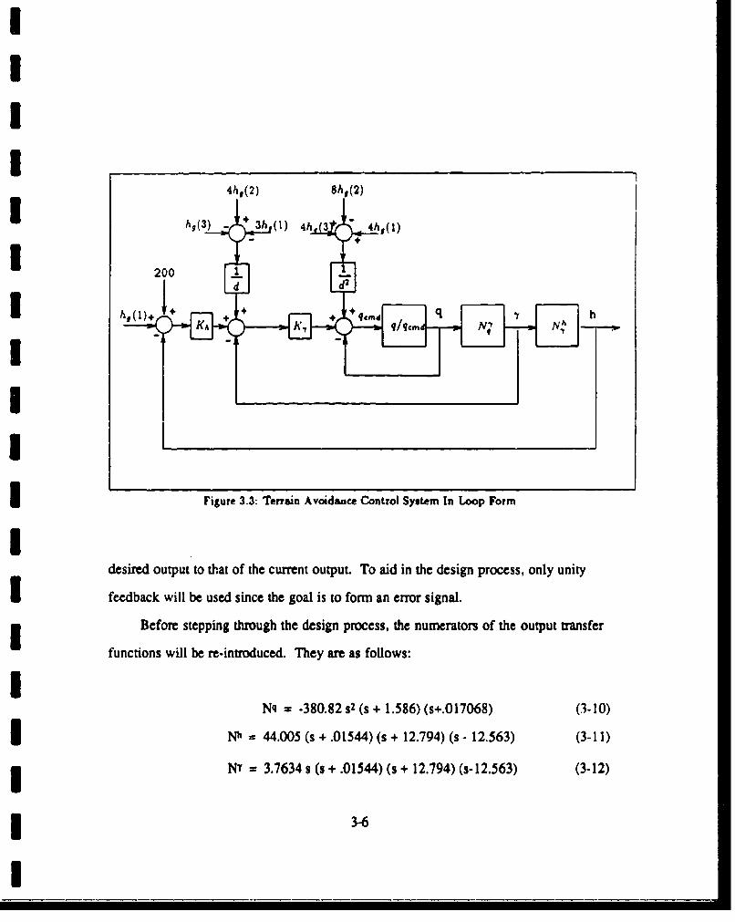
4h,(2) 8hj(2)

hs(3) + 3h (1) 4h 3 0,10)

1 ~2001

Figure 3.3: Terrain Avoidance Control System In Loop Form

desired output to that of the current output. To aid in the design process, only unity

feedback will be used since the goal is to form an error signal.

Before stepping through the design process, the numerators of the output transfer

functions will be re-introduced. They are as follows:

Nq = -380.82 S2 (s + 1.586) (s+.017068) (3-10)

Nh = 44.005 (s + .01544) (s + 12.794) (s - 12,563) (3-11)

NT = 3.7634 s (s + .01544) (s + 12.794) (s-12.563) (3-12)

3-6

I3 Note that both the altitude and flight path angle numerators contain a root in the right.

half plane indicating that they are nonminimum phase in nature. This will affect the

h response of the aircraft to altitude inputs as will be shown in the next chapter.

The design process will begin by closing the inner-most loop of the controller,

which is the pitch rate loop. The open loop pitch rate to pitch rate command transfer

3 function of the controller is identical to the closed loop system that was derived for the

aircraft in the previous section:

I g = 8911.2 s (s + 1.5864) (s + .01707) (s + 1) (s + 5)q(s)cd (s + .01486) (s + .6416) (s + 2.1112) (s + 10.282) (s + 60)

(s + l0)(s + 12) (3-13)[s + (3.3356 t i 3.1843)][s + (15.3023 ± i 15.6413)]I

Since the pitch rate response of the aircraft is already satisfactory, no compensation is

3 required. Therefore, pitch rate will just be fed back to form the pitch rate loop for the

altitude controller:

S_-- 8911.192 s (s + 1.5864) (s +.01707)(s + 12) (s + 10)I q(s).d d (s + .0001 1)(s + .01597)(s + .7691)(s + 1.9061)(s + 10.314)

(s+5)(s+ 1) (3-15)(s + 5.044 ± i 3.1853)(s + 12.136 - i 18.815)(s + 62.958)

i The pitch rate response of the aircraft to a step pitch rate command is shown in Figure

3.4.

Now that the pitch rate loop is closed, the flight path angle control loop can be de-

signed. The open loop flight path to pitch rate command transfer function is formed by

3 multiplying Eq (3-15) by the ratio of Eq (3-12) to Eq (3-10). Figure F.1 shows a plot of

the root loci of this transfer function with no compensation added. The zero in the

right-half plane is not shown due to scaling, however, its presence pulls one branch of

3 the locus into the right-half plane. This has the effect of limiting the amount of gain

* 3-7

I __

.4 ...................... ...................... . . . . . . . . . ... ....................... .,.....................

*. . ......

In

V

V..........----

---

..- . ....................-.---------.......... .....

00 23 4 .

Time (sac)

Figure 3A4 Aircraft Pitch Rate Response to Step PitchRate Command Input

3-8

Ithat can be used to obtain a good response. For this reason, a lead compensator is

required that will pull this branch over into the left-half plane.

The placement of the compensator zero was made such that the new branch

formed on the real axis would attract the branch that originally split and crossed the

imaginary axis. A zero value of -1.80 was selected, and the lead compensator became

Ky = (s + 1.8) (3-16)(s+ 100)

The effect of the compensator is shown in Figures F.2 and F.3. The poles furthest over

in the left-half plane now migrate to the right-half plane zero, and the new branch

formed by the placement of the zero on the real axis attracts the split branch closest to

the imaginary axis. A gain is now selected that will locate the new poles further into

the left-half plane. Figure F.3 displays the position of the new closed loop poles, indi-

cated by the square boxes, for a gain of 200. Letting H represent the product of the gain

I times the compensator and G represent the plant, the closed loop transfer function will

be represented by

Y(s) = GH (3-17)I 1 +GH

SI A confirmation on the effect of the lead compensator is shown by the time response

plot in Figure 3.5. The aircraft flight path angle, y, reaches 90 percent of its final value

in approximately 1.4 seconds which is not outstanding, but does represent a good, stable

response. The nonminimum phase nature of the system can also be seen in the first

0.20 seconds of the response.

3 Now that the closed loop flight path loop has been formed, the outer loop of the

altitude controller can be designed. The open loop altitude to flight path angle

m 3-9

II __I I_ _ _ __ _ _

1.2 ._ _

IL

e-.

0 12 3456Time (sac)

Figure 3.5: Aircraft Flight Path Angle Response toI Step Flight Path Angle Command Input

3-1

U

- o1

command transfer function is formed using the ratio of numerators as previously dis-

cussed, and the root locus of this loop is shown in Figures F.4 and F.5. Note that the

closed loop poles formed in the previous loop become the open loop poles of the current

loop. Once again, due to the nonminimum phase of the altitude transfer function, the

branch of the locus that is closest to the imaginary axis is migrating towards the right-

half plane zero. Therefore, a lead compensator will also be required in this loop if a

satisfactory response is to be achieved.

In order to move the poles that are closest to the imaginary axis further into the

left-half plane, a zero will be placed to the left of the previous compensator zero. The

compensator that will be used is

I + = 2• (3-18)(s+ 100)

This will break the normal pole-zero branch and form a zero-zero branch, causing the

complex-conjugate poles to migrate to the left instead of the right as depicted in Figure

F.6. A larger view of the entire root locus is shown in Figure F.7. The gain selected

for this loop was 15, and the location of the closed loop poles of the system are indi-

cated by the boxes. Forming of the closed loop system is accomplished using Eq

(3-17).

Using Figure 3.6 to evaluate system performance, the time history of the closed loop

altitude controller shows that the system is well damped and exhibits an excellent rise

time of approximately 0.45 seconds. The nonminimum phase portion of the response is

also very evident in the first 0.2 seconds. This controller must now be put in a state-

space format and integrated into the closed loop state-space system of the F- 16 that has

already been derived in Chapter 1I.

3-11

1.2

I .. ...... . . ... ..... ... ... .. .......... '

I V

I.2 ~ ~ ......... • ................ -............... .. • ................ •.................• ................. •...... •.......... •...................

0 .5 1.5 2 2.5 3 3.5 4Time (sec)

Figure 3.6: Aircraft Altitude Response to Step Altitude Command Input

3-12

Controller State-Space Derivation

Once the closed loop system has been derived it is necessary to express it in state-

space format so that it can be combined with the state-space representation of the air-

craft. The reason this must be done is that computer programs for control system anal-

ysis, such as MATRIXx which will be used here, require large systems to be placed in

state-space format (Reference 7). The object of placing the controller in state-space

form is to derive an expression for the pitch rate command to be input into the closed

loop aircraft plant. This is seen more clearly by referring back to Figure 3.2.

If the inputs into the compensators, labeled K, Kq, and Kh, are expressed as error

signals and given the designations y¥., q,, and h,, then an expression can be derived

for pitch rate command:

qd= [K , Kh ] [y., q., h.. ]T (3-18)

The error signals can then be expressed as the difference between the required and

actual value, with the required value being calculated using the derived coefficients:

V= d( [ -3 4 -1] [ hs(l) h,(2) hs(3)]T - (3-19)

q, d-2 [ 4 -8 4] [ hs(1) hs(2) hs(3)]T - q (3-20)

Sh• = [1 0 0 ] [ hs(1) hs(2) hs(3)]T + 200 - h (3-21)

Eqs (3-19), (3-20), and (3-21) can be expressed in matrix form as

yr4'd 1/d /d I1 g1- 0 1 03

q.,, = 4/d2 -82 l/d2 hg(l) + 0 1 0 0 [3-2i- L1 0 0 J Lh(3)J 2 0 U

3 Using Eq (3-22), Eq (3-18) can be rewritten as a matrix that will use the three previous-

13-13Im

ly defined terrain altitudes as inputs and aircraft states as feedbacks:

-3/d 4/d -l/d1 hS(l) . 0 1 0

-qd-= MKY KqKh I 4/d] -8/d2 4/d1 hs(2)j+L0] [0 1j j (3-23)

Lo Lh(3L_ J 0

A state-space expression for the compensators Ky, Kq, and I4 can be created using Eqs

(3-16) and (3-18) along with the, appropriate gains for K. and Kh, which were 200 and

15 respectively. The inputs to the state-space will be the error signals that were derived

in Eqs (3-19) through (3-22):

*X [Z [-1k0] 0 41 0o Lh.- O o(3-24)

yy• -19640 0- Y -200 0 O- ycf

yq -20 0 + 0 1 0 q,

m ~Xhl

y LL 0 -147J " - LJ 0 0 1j Lhj

I The input to the aircraft closed loop plant, i;•j is equal to ,.e sum of the three outputs

from the compensators:

qd Y'y + Yq + Yh

--I = [-19640 -1470[I1 X:+ [ 200 1 15 ] (3"25X [q ff (3-25)

where the express ons for the .rror signals are given by Eq (3-22).

3-14

I, . .. ..... ... . . .. ... .T -T . . .. . .T . ..... '- . .. . . . .T - -- ... . ... .. .. . . i. .. f .. ..-.......- '

Terrain Model and Evaluation Plan

For this study, the terrain model was represented using the downward-facing

portion of a hyperboloid. The equation used to describe the terrain obstacle was

I z = -(x +y 2)/4000 + 1000; 05 z5 1000 (3-26)

where

z = terrain altitude (ft)

x - downrange distance (ft)

i y = crossrange distance (ft)

A three-dimensional view of the terrain model is shown in Figure 3.7. Since the eval-

uation will only be performed flying over the top of the hill, the crossrange distance, y,

will always be equal to zero.

!FI

i Figure 3.7: Terrain Obstacle Model

I3-15

I I I II I II I II I II

Now that the pitch rate input into the closed loop aircraft plant has been expressed

in terms of the three terrain altitudes and three state feedbacks, aircraft performance

will be evaluated for varying values of look-ahead distance, d. Distances of 0, 300, 600,

and 1200 feet will be used to determine if this is a good approach to the terrain avoid-

ance problem. The results, which are addressed in Chapter 4, will be evaluated using

plots of aircraft altitude versus ground distance. Digital terrain models will be simu-

lated by biasing the terrain altitude as a function of distance. For example, a terrain

model with a look-ahead distance of 300 feet would contain the normal terrain, labeled

hg(l), a second terrain input that is placed 150 feet closer to the aircraft, called hg(2),

and a third terrain input that is placed 300 feet closer to the plane, which is designated

as hg(3). This concept is shown in Figure 3.8 which is an enlarged area of the initial

upslope of the hill. Moving the terrain closer to the aircraft is the same as looking

farther ahead of the aircraft, therefore, this is the approach that will be used for all look-

ahead distances.

S00

700................ ... ....... .. ..... ......... .......... .---0 ...... .... . .. . ... .. . ........... ........ ............ . ..... ...... .. .. .. ... . . ... ....... . .. . . ... ..

5 0 0 ! ..... ..... .. ..... .... ... . .. ... ..... . .... . . ........ .... ........ ......... .. ..... .......

C o o0 0 .. ......... .............

..4 0 0 . ................... ........... ... ..... ...

3 0 0 ....................... ... ................. ...................... • ...................... /0 ......... ...... .

2 0 0 .. .. .. ... .... ... ... .. .. ... .. .. .. ... .. .. .. .. .. ... .. ...... . ... ..... .. .. . ... .. ..

0 . . . .-.-. . .0 500 1000 1500 2000 2500 3000

DiOtance (ft)

Figure 3.8: Enlarged View of Simulated Terrain Showing theConcept of a 300-foot Look-Ahead Distance

3-16

I- l____ I _IIII_

I

I IV. Resilts And Discussion

Altitude Controller Evaluation

The altitude controller, designed and implemented in Chapter III was evaluated

fo: five values of look-ahead distance: 0 feet, 100 feet, 300 feet, 600 feet, and 1200

I feet. Each distance was evaluated against the terrain model which was developed in

Chapter I3. The evaluation and comparisons made between the various look-ahead dis-

tances were based on the altitude response of the aircraft with respect to the terrain.

The first distance evaluated was 0 feet, therefore hg(3) and hg(2) were equal to

zero. This case is representative of the use of radar altimeters, which essentially look

downward from the aircraft to obtain information on terrain altitude. Attack and small

fighter aircraft such as the F-16 and A-10 use radar altimeters for this purpose. As can

I be seen in Figure 4.1, the aircraft did not avoid the terrain due to the sharp rise. This is

similar to using a radar altimeter, not including the altimeter cone model, for terrain

avoidance. Over gentle terrain, the radar altimeter will work well as a sensor because

the lag time between sensing of the terrain and aircraft response is small compared to

the rate at which the terrain rises, thus providing the aircraft with ample time to

I respond. Even though the aircraft had problems negotiating the initial terrain rise, it

did reach the desired peak value of 1200 feet MSL, or 200 feet above the terrain peak

and followed the backside of the hill rather well. Using Figure 4.1, the lag time for

aircraft response can be measured as approximately 0.5 seconds which corresponds

with the rise time that was observed in Chapter III for a step input.

The next distance evaluated was 100 feet, which corresponds to the value of

hg(3); hg(2) took on a distance of 50 feet for this case. All three loops of the altitude

controller will have pitch rate inputs. Figure 4.2 shows the results of this test distance.

Again, the F-16 crashed into the terrain obstacle, but a very slight improvement in

* 44I _ _ _ _ _ _ __ _ _ _ __ _ _ _ _ _ _ _ _

* 1600

i1 4-0 0 ....................................... . . . . . . . . . .--......... .......... •................... ............ ............................

1 2 0 0 ................... : ................... i....................i .... ........ i.. ................. ................... ................. .1 0 0 0 ................... i........... ........ .. .. ......... .. ........... i..... ... . . . . .•. . . . . . . . . .

i ~~ ~ 0 /......... --------.............. ....... i................. ................... ..................6 0 0 ...... ............. ................... .. . .............. . ................... .. ..... ...... ................... i...................

4-0 0 ... .... ... .... .... .... . ................ ... ............. ......... ..... .... .. .. .... .. .. .. ........

2 0 0° .• ................... .............. ........... I..... ....... ........... . ,

200

0 5 10 15 20 25 30 35

I Time (sac)

I

I Figure 4.1: Altitude Response vs Terrain for 0-foot

Look-Ahead Distance

44-2

I

3 40

1600

1 4 "0 0 ................... ....................................... .................... ....................................... .......... .........

1 0 0 0 ................... " . ......... . ....................". ..

18 0 0 .. ...... ... .. .. .... ..... . ./ .. ..... ........... . ...... .......... ................... .. ........

".. ... ..0.. ................ ..... . ... ..... ... . . . . .......... ....... ........................I 00< <.,~

4 0 0 ...................................... ......... ..... ................. ....... .. ....... . . ............. ......I400 .................... " •i

2 O00, ....................... ................ ............... ...... . ....... ............

I I .

00 5 10 15 20 25 30 35

I Time (sec)

Figure 4.2: Altitude Response vs Terrain for 100-foot

Look-Ahead Distance

4-3

I

response can be seen. Referring back to the flight path angle response in Figure 3.5,

one can see that the flight path loop of the controller would not have ample time to

build up a significant input value. A 100 foot look-ahead distance for an aircraft travell-

ing at 670 feet per second only corresponds to an additional 0.15 seconds of response

time. Therefore, not much improvement could be expected for this case.

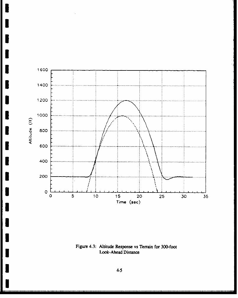
The next look-ahead distance evaluated was 300 feet. Although the aircraft still

penetrated the terrain model slightly, it did show a significant improvement over the

previous two cases. Figure 4.3 illustrates these results. The initial response of the

aircraft occurred approximately 0.5 seconds prior to when the altitude loop began feed-

ing inputs into the system which should be expected for a 300 foot look-ahead distance.

However, the initial response was in the wrong direction due to the nonminimum phase

nature of the flight path angle loop. Still, the overall response was an improvement in

comparison to the 0 and 100 foot cases.

The nonminimum phase response of the flight path angle loop was more pro-

nounced for a distance of 600 feet since there was twice as much time available, com-

pared to the 300 foot case, before the altitude loop commanded inputs. As shown in

Figure 4.4, the F- 16 just barely avoided the terrain due to the larger look-ahead distance.

The nonminimum portion of the flight path angle response subsided approximately 0.5

seconds before the aircraft reached the beginning of the terrain obstacle, giving the

aircraft a slight amount of positive pitch rate.

As with the all of the previous three cases, the aircraft reached a maximum al-

titude of 1200 feet, or 200 feet above the terrain, as was desired with the peak altitude

occurring closer to the peak of the terrain. This indicates that the implementation

scheme is working as intended since information about the upcoming terrain is obvious-

ly being used in the calculation of the pitch rate command input.

I I4II4

II

I

I3 1400

1 4 .0 0 ...................................... .................... ........................................ ........................................

312 0 0 ........ ......... ......... .....1 0 0 ............. .i.... ............... .... .......... .. ..... .. .......... .................. .. i .................. ....................30 0 ..................0 0 ............*-....... .................. ........... .......................................

" 6 0 0 .................. ................... .. ..................... ..... ................... ...................

I • ! i ~/ . ,

400~ ~ ~ ~ ~ ~ ~~~~~~~~~~~~... .......... I........................................... .. .............................I - eo......... ........60 0 . ............................................ ....

400.i ~ ~ ~ ~oo~~~ ....L....L....L.....J,..... L..L.......L ..... ........ J ........... t...... ........ ........ L......L...L.. J L~............. ', \ ......... ...........

0 5 10 15 20 25 30 35Time (sec)

iI

Figure 4.3: Altitude Response vs Terrain for 300-footLook-Ahead Distance

I 4-5

I _ _ _ _ _ _ _ _ _ _ _ _ _ _ _ _ _ _ _

I 1600 .

I1 0 0 0° ...................... ........ . .... . .. .. ... ... ... .. ...... .

1 2 0 0 ................... ............... ....................... T... .... ......... . . . . . . . .................... I...................

4 00O O .................. .. ..... ... .................... ................... , .............. .. ........ i........... .........0 5200

I 40 0 ..............................

-4-

III

I I I .L........I.......... ...... L.\...A.. ~ .J.L I...L..L..L.J.

0 5 10 1,5 20 25 30 35i Time (sec)

I

I Figure 4.4: Altitude Response vs Terrain for 600-footLook-Ahead Distance

The final look-ahead distance evaluated in this thesis was 1200 feet. Dramatic im-

provements in aircraft altitude response were evident as can be seen in Figure 4.5. The

F-16 nearly followed the entire terrain obstacle using the 1200 foot distance. Although

the portion of nonminimum phase response is slightly longer, the amount of pitch rate

built-up by the time the aircraft reached the beginning of the terrain negated the rise

time delay for the altitude loop that was seen in the earlier cases. Also note that the

larger look-ahead distance decreased the overshoot of the 200 foot target altitude at the

end of the terrain avoidance maneuver.

In order to achieve a better feeling for the spatial relationship between the aircraft

and the terrain, Figure 4.6 has been included to show aircraft altitude as a function of

downrange distance from the initiation point of the test run. The aircraft required ap-

proximately one mile of distance to fly over the 1000 foot high hill.

To confirm that the flight path angle was the cause of the initial nonminimum

phase response of the aircraft, a test case was run with all of the gains in the flight path

loop set to zero: in other words, only the altitude and pitch rate loops of the controller

were providing pitch rate inputs into the aircraft flight control system. As suspected,

the terrain avoidance performance of the F-16 degraded significantly in the absence of

flight path controller loop inputs, which can be seen in Figure 4.7. The performance of

the aircraft with a 1200 foot look-ahead distance is very similar to the 100 foot case,

and this indicates that the pitch rate inputs are insignificant at longer distances. Refer-

ring back to Figure 3.2, the reason pitch rate inputs become insignificant at large look-

ahead distances is due to the I/d2 term that is present after the summing junction for

the altitudes in the pitch rate loop. Therefore, it can be postulated that a first order e-

quation probably would have performed just as well as the second order one used in this

study.

4-7

I ____IIIII_

IIII

I 1600

1 4 00• o ..................... ...................................... .. .................... .. . . . .. . . . ....... ...... ................... . .

1 2 0 0o ...................i ....... ............ !................... : ........... i ................. i ................... i ........... ..... .I 0 0 .................. i. . . . . . . ..... ... 1 ... ..... .. . ...... .............. ................. .. ...... ......

I °I1 600 ... ... ... ..

I 200

I

0 5 10 15 20 25 30 35Time (sec)

II

Figure 4.5: Altitude Response vs Terrain for 1200-footLook-Ahead Distance

I 4-8

i

III ~ ~1600 - -

100........... ........ ..........

1 0 0 ........................... .. ...1 .. / ,..

" So .. .. ... .. . ...... .... .............. ............... .............. ... .. ......... 4. . . . . . . . . . . . . . . . .

I " o o o :6 0 ............................... .... . , ......... .. ................ .. ... .. .... ................. .......

, o :................................ . . u .......i ................. ! ................ i.........• ................. !..................4 00 .... ..l ....

2.0 0 . ... .... ............. "................. I ................ ............. ... ......

II: l

I 200

0 1000 2000 3000 4000 5000 6000 7000 8000Downronge DiMsonce (ft)

Figure 4.6: Altitude vs Range for 1200-footLook-Ahead Distance

4-9I . . .. .T ]... iI l -i -.. .. .] .. • . .i • .. .. -

IIII

3 14.00 -

I 120

31 0 0 0 .. ............ ..... ... .......... ......... ...........8 0 ..... ........... .................. ....... .. . . . .................... . . . . . . . .

00 ............. ......... ....... ..............

I 400 ................... ............... ........... ...

.. . .. . .. . .. . , . . . ............ , ....... ., . . . . .. ................ , ....... ........... ,....... ........ ............. . . . .

"0 'j

I0 5 10 15 20 25 30 235q Time (sec)

SFigure 4.7: Altitude Response With Reduced Gain in Flight Path

Loop for 1200-foot Look-Ahead Distance

4-10

I00

m One of the constraints placed on the terrain avoidance problem in this study was that

the aircraft could not exceed t 4g of incremental load factor or -3g : An < 5g. As seen

in Figure 4.8, incremental load factor, represented by the dashed curve, reached a maxi-

mum value of approximately 2.7g which corresponds to an actual load factor of 3.7g.

Aircraft pitch rate response is also shown in Figure 4.8 along with altitude response

m versus terrain; the altitude response is shown as a reference for correlation purposes.

Figure 4.9 contains the time response plot for horizontal tail deflection during the

terrain avoidance maneuver. As can be seen, the deflections did not exceed the limits

of t 25 degrees, and reached a maximum value of almost 8 degrees.

Figure 4.10 contains a comparison summary of altitude error for each of the five

look-ahead distances evaluated. Note that the altitude error becomes smaller as the

look-ahead distance is increased, which is what was desired. The line corresponding to

-200 feet of altitude error represents the terrain, therefore, any curve falling below that

line indicates that the aircraft impar-d the terrain. While the 1200 foot look-ahead dis-

tance does show a significant ir, -. nent over the other distances evaluated, it still

3 has wide variations in aititude error (-105 feet to 140 feet). For this reason, an experi-

mental test case was carried out using an approach that was slightly modified from the

m one presented in this subsection.

Alternate Terrain Avoidance A•proach and Evaluation

An alternate approach was tried for implementing a terrain avoidance system to

see if any improvements could be made to the altitude response of the aircraft. Refer-

ring back to Figure 3.6 which shows aircraft response to a step altitude input, one can

see that it takes approximately 0.45 seconds for the aircraft to reach the value of the

I commanded input. This lag time roughly corresponds to a distance of 300 feet given a

velocity of 670 feet per second. Therefore, if the aircraft receives terrain information

m 4-11

I_

1400

I 000 ......... .... ..Bo .... ....... 0...... .5 20 25.... 30........

0

0 5 10 15 20 25 30 3 57Tin) (sec)

I igre48:Aicrf Pitch Rate andeLoad FatrRsosvsTrri,()PthRean Load: Factor Resons

I 4-12

I 0 1 02 03

IIIII

I........... .. ...... ...... ... ....... ..............

o . ....................

I o°

o 2 -

I " - 2 . . . . . . . .................... .................... .................. .. ....................................... .

... -- 4 ...... ..-. .... ....0 .

5 10 15 20 25 30 .35Time (sac)

mI

Figure 4.9: Horizontal Tail Response for Terrain AvoidanceManeuver With 1200-foot Look-Ahead Distance

I 4-13

I _ _ _ __ _ _ __ _ _

.300

0 ft- 100 ft

.. 300 ft2 0 0 ....... .................... .6 0 0 f t ..... .

* - 1200f t

1 0O 0 ............. .................... ................. ........... ...... ............. ............ .. .... .... ..... ...

o / :

LU 0 .

' I-IN'• - 1 0 0 ................. ;..................... .. . ...... •... ....... .. .................. .............. .......................

" j• i

/"

- 2 0 0 .. ... .. ......... ... . . ....... .... ..................... ..................... ..............

-300 --0 1000 2000 3000 4000 500 0 7000 8000

Downrange Distance (ft)

Figure 4.10: Altitude Error vs Range for Various Look-Ahead Distances

4-14

.. ..- --

I terrain

VI7 f/

300ff ;t O.45aec

u Figure 4.11: Alternate Method for Implementing Terrain Avoidance

4-15

300 feet in advance, it should be at that terrain altitude plus 200 feet by the time it ac-

tually arrives at that point in space. This approach is illustrated in Figure 4.11. If the

initial conditions of the aircraft were different, all that would need to be changed is the

look-ahead distance. For normal operating airspeeds, look-ahead distance would be

proportional to horizontal velocity. At slower airspeeds, this distance would need to be

increased since load factor capabilities degrade in this operating regime.

In implementing this approach, the system which had already been developed can

be used with a few minor modifications. The look-ahead altitudes referred to as hg(2 )

and hg(3) in the previous section will now be set to zero, as will the hg(l) input to the

pitch rate and flight path angle loops of the controller. The only point in the loop where

hg(l) will be input is in the altitude loop of the controller. What is actually being done

is to make the aircraft think that the terrain lying 300 feet ahead actually lies below.

The time response for aircraft altitude versus terrain altitude is shown in Figure 4.12.

Comparing Figures 4.12 and 4.5, several conclusions can immediately be drawn. First,

the total time required to traverse the terrain is about two seconds less using this ap-

proach. Second, the nonminimum phase response of the aircraft is eliminated since

flight path angle is no longer commanded which results in a quicker overall response.

Third, peak aircraft altitude occurs closer to peak terrain altitude using this modified

approach. The results from implementing this approach show that the aircraft altitude

response produced less altitude error compared to the error produced using the 1200

foot look-ahead distance, as is shown in Figure 4.13. Altitude error remains within

about t30 feet using the modified system compared to the 1200 foot look-ahead distance

error which ranges between -105 feet and +150 feet.

Examining the pitch rate and incremental load factor response, seen in Figure 4.14

indicates that actual load factor momentarily exceeds the 5g limit by reaching 5.5g.

This is a much more aggressive response compared to the response seen using the 1200

4-16

foot look-ahead distance, which accounts for the decreased amount of time required to

traverse the hill. The increased response can probably be attributed to the fact that no

commanded inputs are coming from the flight path angle or pitch rate loops of the con-

troUer. Using a 1200 foot look-ahead distance, these two loops will begin commanding

negative values of pitch rate while the aircraft is still climbing up the front side of the

terrain, thus decreasing the overall commanded pitch rate and resultant load factor.

I However, they do have a distinct advantage during the initial response to a terrain

* obstacle.

.: a ......................................... .. . .. . . ..................................................... ............. .1430. .

1000 ........... . ".

S~/ I

800......................4 .\

60 0~ ~~~~ ~ ..... ....... ............. ... .| . ..... ................ ...

46 0 0 . .................. • ............... ... .. I*............... . .................. . ......• . .. .. . ..........

2 -0 0 1.. . . . . . . . . . . . . . . .A . . . .... ................ ...'.

. . . . . . .. . . ..

II

0 5 10 15 20 25 -0

Time (sec)IFigure 4.12: Aircraft Response Using Modified Approach for 300-foot3 Look-Ahead Distance

3 4-17

I

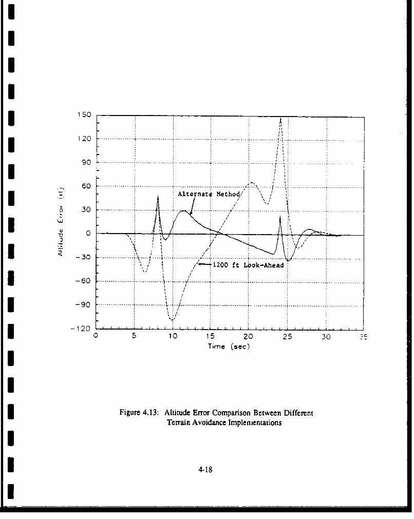
III

i 1 5

1 2 0 ............. ....................... . . ....................... ...... .'. I

9 0 ~ ~~ ~~~~ ~ ~ ~ ~ ......... .. .. . .. .. .. . .. .. .. ... .. .. . . .... ............. -• , ........................ . . . . . . .

I 90

.. . ...... ........ ... .... .. . . . .. . ........... ........... ......... ............. -- - - - - ... |.. ... . ... ......... ........ . .. . . .

AlternatO Method/

SL,

0 PP

I <-30

I /1200 f t Look-Ahead:

-620

I -90

I0 5 10 15 20' 2'5 30Time (sec)

Figure 4.13: Altitude Error Comparison Between Different

Terrain Avoidance Implementations

I 4-18

I _ _ _ _ _ _ _ _ _ :_ :_ _ _ _

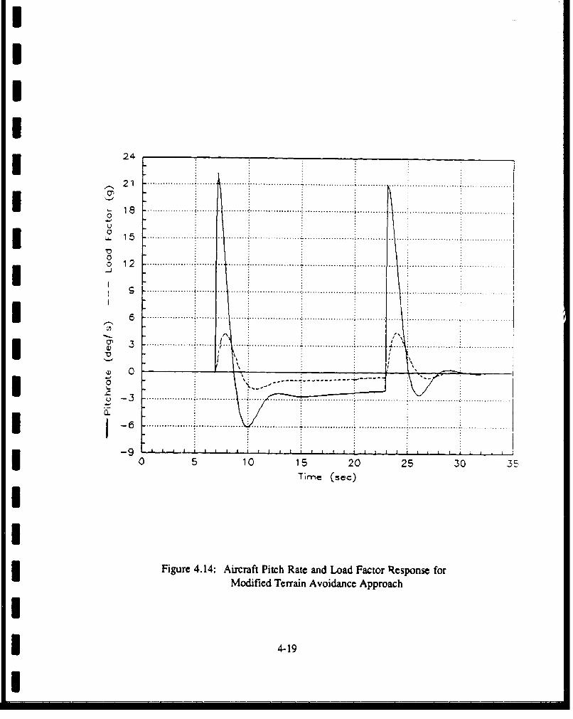
III

I

.• 2 1 ................ .......... .......... .................... . ............. .............. .... ... ...... .. . ...... ......

. ............ ..... . . ... ....... ....... .. ............. . .. .....

0 1................. ........ .....................15 i

:

0 1 52 ............. .. ........ ................... ............ .............. ... . . ................. ................... .

I"I £ . ... .. .. ... .. •.. .. . .. .. . . .. ............ . .................. .. ....... . ... . ... ................... ... .. .. .. ..... .. .

. ..... ...... .....I 6 *t

3 ............... .. . ...... . .. ................... ... • .................... • ......... . . . .. .. ............... . . .. . . .

I9 1 1 .•

"0 5 10 1 20_25__0__@ 0 ::"

4-1

0

-... " .............. .................... ................I....1 -.. .. . .. .. . .. .. . .. .. . .. .. .

I0 5 10 15 20025 3Time (sec)

II

I Figure 4.14: Aircraft Pitch Rate and Load Factor Response for

Modified Terrain Avoidance Approach

II~4.-19

I__

I12

1 ................... ......... .... .................... ................... i..................... ................... ...... ..............S8 .................. . . ..... . , .................... !..... ............... ................... i................... ,. ................ .

I

I-

6 .................. .... .. .......... ............... 7 .. ..................... ; ........... .. ................. . ...................

I..... ..2..... . ..__ __ _ _ _

...0.. .. .. .. .. .. .1.. . . . . .. ....... .....

C

- 2

0-

0 ..4

I ~-6I6 .... .. .... ... .. .................. ......... . .............. ..........

...1 .........L . ..... ..... .. ..... .......J..L . .1 ..L.........L .L.....L....L.. I..... ..... L....L....L...A . L. .. . .

0 5 10 15 20 25 30 35Time (sec)

I

Figure 4.15: Horizontal Tail Response for Modified TerrainAvoidance Approach

4-20

1I Y

Based on the results presented in Chapter IV, some conclusions can be reached

about the effectiveness of each of the two terrain avoidance schemes: one based on

three different reference altitudes using a look-ahead distance, and the other simply

based on information about the terrain lying 300 feet ahead of the aircraft. Some con-

clusions can also be drawn about the potential of the digital terrain database with

I respect to ground collision avoidance systems.

Using the altitude controller that was derived in Chapter IH and evaluated in

Chapter IV, a minimum look-ahead distance was required in order for the aircraft to

effectively avoid the terrain. A look-ahead distance of 600 feet provided enough ad-

vance terrain altitude information for the aircraft to just avoid terrain impact. Using

I the original approach of utilizing three different terrain altitudes, the only look-ahead

distance evaluated that provided sufficient altitude separation between the aircraft and

the terrain was 1200 feet. Even then, the altitude error had a variation of 255 feet be-

tween the minimum and maximum error values. The design did return the aircraft to

the initial conditions of level flight and 200 feet in altitude after traversing the terrain

I obstacle, as was required. The alternate approach of looking a set distance ahead of the

aircraft provided a better terrain avoidance capability.

A defect in the design of the terrain avoidance system was the response of flight

path angle in the altitude control loop. While it was a good idea in theory for the

purpose of aligning the aircraft velocity vector with the slope of the terrain, the flight

path angle loop of the controller exhibited a nonminimum phase response which gave

the controller some drawbacks. However, the flight path angle loop greatly enhanced

aircraft response when larger look-ahead distances such as 600 and 1200 feet were used.

For shorter distances, this loop was ineffective due to a somewhat sluggish response.

* 5-1

S I

An attempt was made to use pitch angle, 0, instead of flight path angle for following

the slope of the terrain, but this design proved ineffective because a change in pitch

angle did not produce an equivalent change in flight path angle. The result was aircraft

impact into the terrain. The pitch rate loop was ineffective for any reasonable look-

ahead distance because of the squared distance term in the denominator of the forward

path gain.

All of these factors, when combined, resulted in very little improvement in the

terrain avoidance capabilities of the F- 16 for look-ahead distances less than 600 feet. A

redesign of the flight path angle and pitch rate loops of the controller could result in

better response characteristics for the controller, however, it is questionable if the over-

i all performance of the terrain avoidance system would improve. Satisfactory perform-

ance could be achieved for distances greater than 1200 feet.

The performance of the alternate terrain avoidance implementation showed a dra-

matic improvement in the capabilities over the system that was just discussed. The

I altitude errors of the terrain avoidance system were reduced to -30 feet by converting

* the rise time of the altitude control loop from seconds to a distance and moving the

terrain reference point this distance out in front of the aircraft. This sort of implemen-

tation was a more intuitive approach to implementing a ground collision avoidance

system. This design also returned the aircraft to the initial conditions of level flight

-- and 200 feet in altitude after traversing the terrain obstacle, as was required.

The terrain avoidance system that was designed for this study was based on only

one condition. For other flight conditions, or off design cases, the required look-ahead

distance will change. Look-ahead distance should be increased for faster airspeeds and

decreased for slower airspeeds up to a certain point. At flight conditions where the

maximum allowable load factor cannot be achieved, which was 5g for this study, the

look-ahead distance will need to be increased in order to allow the for the slower

I 5-2

I

response time of the aircraft at the reduced maximum achievable load factor. The pro-

blem of implementing a variable look-ahead distance could be accomplished using a

schedule similar to the variable control system gains that are based on impact pressure.

Both of the GCAS implementations discussed in this thesis made use of potential

of the digital terrain database (DTD). Obtaining terrain information at a series of dis-

tances in front of the aircraft is a task that is tailored to the capabilities of the DTD.

Using the DTD, this distance could be varied according to flight conditions. In addi-

tion, information on the surrounding terrain could also be obtained at the same time

without the use of a dedicated sensor meaning a GCAS could be designed to maneuver

in the lateral-directional plane. The DTD will most likely be an integral part of any

future terrain avoidance system.

5I

II

I

I 5-3

I

I

SVY_. Recommendations

During the course of this thesis, several additional areas of interest have emerged

which should be evaluated. Each of these areas of interest have the potential for advan-

cing the solution of the terrain avoidance problem. These areas are as follows:

1. Implementation of the two terrain avoidance systems

N developed in this thesis into an F- 16 simulator so that a

b more detailed study can be conducted on the effects of

look-ahead distance on terrain avoidance capabilities.

An investigation could also be done using f,;,id sys

.d tern that combines the features of both systems used in

this thesis.

1 2. Developm'nt of a three degree of freedom ground

* collision avoidance system which can maneuver in the

lateral-directional axis in order to avoid terrain.

3. Develoment of a terrain avoidance system using opti-

mal control theory for determining the path for mini-

I mum distance or for minimum time around a terrain

obstacle.

The first recommendation is required in order to validate the results of this thesis.

A study should be done to determine the effects of look-ahead distance on terrain avoid-

ance capabilities and what the required minimum distance is. Different terrain obsta-

cl, and slopes should also be used in order to determine their effects on terrain avoid-

ance performance. Several F-16 simulations are available at the Flight Dynamics

Laboratory and can be connected to terrain boards or digital terrain databases. The

simulations are written in FORTRAN computer code and would require modification

* 6-1

I ___

I3 in order to incorporate the altitude controller developed in this thesis. Using results

from the simulator, a comparison could be made to ascertain the potential of the terrain

avoidance systems developed in this thesis.

The second recommendation was made because no current, automatic GCAS

I design incorporates maneuvering in the lateral-directional axis. This is an area that has

considerable potential in the tactical combat arena since maneuvering in the longitudi-

nal axis can often increase aircraft exposure time to enemy defenses. Maneuvering in

the lateral-directional axis could have the potential of using terrain obstacles to mask

the aircraft from enemy radar. In addition, this could enhance the terrain avoidance

I performance of the aircraft in mountainous terrain where vertical pull-up maneuvers

may not 'w effective at low altitude.

If this recommendation were pursued, some sort of bank angle hold loop would be

required since, as shown in Chapter 2, the F-16 state-space model could not maintain a

non-zero bank angle. An alternate approach to this problem could be the addition of a

I lag compensator that would force the spiral mode root closer to the imaginary axis, thus

slowing down the effects of this root on roll rate performance. Presumably, if this

problem were overcome, then a variation of the altitude controller developed in this

3 thesis could be used since the look-ahead distance vector would be translated through

the pitch angle and bank angle.

The third recommendation involves a complex area of control theory. Using the

terrain obstacle developed in this thesis, optimal control theory should be able to define

I the minimum time or minimu.n distance path around the terrain along with the optimal

control law for the pitchrate and roll rate inputs required to fly this path.

Using pseudo 'baug-bang' control for pitchrate inputs of -11 degrees per second, a

3 time history of aircraft altitude versus terrain altitude was generated. This time history

and ihe time history of the other aircraft states are. shown in Figures 6.1 through 6.4.

I

I

II3 Figure 6.1 shows that the time required to traverse the terrain obstacle is slightly less

that 14 seconds compared to a time of approximately 18 seconds from the system eval-

uated in this thesis. Since Figure 6.1 is using the maximum pitchrate authority limits,

this should be close to what optimal control theory would predict.

Another approach using optimal control would involve designing the altitude

I controller using loop transfer recovery techniques. This involves setting up a linear

quadratic cost function with weightings on the aircraft states and penalties on the

I controls. This approach is used for the infinite horizon problem where time is not a

constraint, and the solution to the optimal control problem is based on the solution of

I the Ricatti equation.

IIIIII

II

I

1 6-3

I _ _ _ _ _ _

IIIII

3 ~ ~1200. -____ __

I 10 0 0 ............................................. . ............................................ ................

800 ......... .............. . . ...... ......... .....

0 0 . . .. . . . . . . . . . . . ........ ... ................. "•.... •.......... ............. . . . . . . . . .. ; . . . . .. . .

I ."/ %

2 0 0 ........ . . . .i................. .. . . . , . . ..i ............. . . . . ..... .. ....... .......... ,............... . . . . . . . . .

Si I

I00 ~ 4*/ 6 8 0121

Fgr 6.1 Tim Hitr'fF !6Tranviac

U 't

:I :0 2 4......0.12.14..16Tim (: "

Figur 6.1: Time HistrofF1TerriAodac

3 Using 'Bang-Bang' Inputs

I

IIII

3 1200

I 10 .. ;

4 00° ° .......................... ............. .......... ....i" ..... ..... ... ........ f.............................. .

, i ,

2 0 0 ................ .......... t . ............. ... ......................... ..............................

*I

00 2004.0/0080 00

, .S600 .444,

I 0 . . . . . . . . . . . . .. . . . . .. . . . . . .. . . . . .

I

|/ ,II

I0 2000 4000 6000 8000 10000

Down-Range Distonce (ft)III

Figure 6.2: Aircraft Altitudc vs Range Usi-, 'Bang-Bang' Inputs

I3!6

!

S10 ... ...... 4.

3 10

5 .. .. .. .... .............. . .... .... ........ .(D1

Qj 0 0

o 0)0-2i ........... ............ .I CL

- 1 0 .. ... . -. ................

0 5 10 15 20 0 5 10 15 20

Time (sec) Time (sec)9 (a)._3 (b)

-6 .. . ..........--- 10

3o ...... . ... .... 1 0 :

0 0- 3 .. .. .. ... .. .. . ........... .. .. . ..... ..... I ... ........ ...... .....

- 6 o. 20 ....... ...... . ......... ........ .- 9.......... ......... ..... ... .

0 5 10 15 20 0 5 10 15 20-rime (sec) Time (gec)

(c) (d)

I

I Figure 6.3: Aircraft State Responses for Terrain Avoidance With'Bang-Bang' Inputs: (a) Pitch Rate, (b) IncrementalLoad Factor, (c) Angle of Attack, (d) Pitch Angle

I ,6-

I

I -15

-150246810 ....... .......... 4... ....... 6.....

E0

10 .........i...... .4......... ... ........... ............. ........ 4 ....... ........

0 24 8 10 12 1.4- 16Tirme (sec)

Figure 6.4 Aircraft Pitch Rate Response vs Pitch RateCommnand for 'Bang-Bang' Inputs

3 6-7

Appendix A: F-16 Control Derivativesand Trim Conditions

This appendix contains the aerodynamic data used to created the state-space system

for the F-16. The data shown on the following page were obtained from test flights of

the Advanced Fighter Technology Integration (AFTI)/F- 16 technology testbed

demonstrator aircraft. While it does have several features that are different from the

production F- 16, the AFTI aerodynamic data is representative of the normal F-i16. It

should be noted that the AFTI has a pair of canards mounted on the engine inlet that are

I 15 degrees off vertical, however, their effect on the aerodynamics of the aircraft is

negligible.

Pages A-3 and A-4 of this appendix contain the values of the various longitudinal

and lateral-directional control derivatives in both the stability and aircraft body axes.

Values for body axis derivatives are given in both dimensional and primed dimensional

I format. For a discussion of the differences between the two forms, reference Appendix

D. Primed dimensional derivatives were used in the construction of the state-space

system.

A-I

INI0

I~N'

ey a

0 0e0; dD 0 .

VI Ub

4- - j0 4 -I

U 2

-xw

A W

L r* CD Ln'a tv P lT I 0 ID 4

CC w ~ ' 0 C C C

-~ 0 N

6; 4C5C Ci NI IVC I

LL~ 4L M [A rY N JI-ý - N O

.as -9 , 4 2 N; - F, s =

*D CD r 0 4e co 4

*c -j > - ~

- a.- -ý j . a L

0'9 cc~" W

X, C.c

* A-2

IIIII CD - .21,•¢¢¢,•¢¢,¢¢•s¢¢$¢$¢¢t

Lc NG I ruDINAL srAsILITY AXIS COLFFICIENTSIALPHA ci .54671

L: L. I l.€L C M = •JJO•CD a • 7 1E 0

= . 71.'799.'E-ul CMA = .4898(:0'cE-02 CDA = .152400E-02'.LDE = .899700E-02 CMDE •:-.)99cE-(:,- CDDE = -. 258,8000E-07,iLDF = .I52'E-h1 CmD 951 = -. 55o(E(.E-)-, CDDF = .645000E-lC

CLO - 2. 77% CMO =-2.59581ICLkU 2 -. 948273 CMAD = -. 789587CLU x -. 12.000E-'4 CMU w -. 420000E-04 CDU - .80000()E-05s *a*Ea•¢g¢s¢sss*$ses$gs**g¢s**s***s*$********s•sw**

IS THE ENTERED DATA CORRECT ? (YES./NO)YES

LONGITUDINAL BODY AXIS COEFFICIENTS (1/RAD)CZ - -. 131540 CX - -. 182371E-01

CZA - -4.08122 CMA a .280531 CXA = .152704CZDE a -. 514674 CXDE .'86847E-01CZDF s -. 869400 CXDF - -. ±34941E-O1

ICZO w -2.'646 CXO - .6ý0881E-01CZAD • .947582 CMAD = -. 7892q9 CXAD - -. 255862E-Ol

CZU - -. 152964 CMU a -. 761680E-02 CXU - -. 406192E-01

LONGITUDINAL AXIS QIMENSIONAL DERIVATIVES-Z = -:1619.9 M = .000000 X = -2914.27

ZA 0 -999'.14( MA = .41895 XA - •7.3841

ZDE = -126.0') MDE - -19.0854 XDE - 7.0224:DF w -- 212.8141 MDF - .1.897 XDF = -37.355ZO L-• - 4. 8 ý5d' .))MQ -. 736707 X 0 .130552

ZAD a 1.U90?0 MAD -. 224008 XAD - -. 52947"E-01ZU a -. 559257E-1 MU- -. 381925E303 XU -. 148509E-01

LONG BODY AXIS PRIMED DIMENSONAL DERIVATIVE$ZA' -1.41F214 MA' 9.75321 XA= 37.3841

ZDE' -. 188171 MDE' - -19.0412 XDE' - 7.02243ZDF' * -. '17864 MDF"' -1.76596 XDF' - -3.30355ZO' .992779 MG' * -. 959097 XO' - -17.9453ZU' a -. 835210E-04 MU' -. 363216E-03 XU' - -. 1485(19E-01

ZTHETA - -. 129799E-02 MTHETA' a .290760E-03 XTHEIA' - -32.1688

IiIA-3

IIIII

I ss¢¢ .*¢se*.t s$gti~ss s*$$t *€•w s**$$!$$$ *ss**$s

LAT- IFR TA•iLIT' AUS C EFFICI NTSCN• = .1'•1':,5-,'> 2 CLI' = -. L6,'BOQE-C'2 C'fE = -. •',,.-,

CNF = -. 46ob(:f:E-02 CLP -.=2:17:9 CYF = 5141-,E-ICNf = -. 47-181 CLR = -. 4990'v."E-,E2 CYR - .57411

CNrD = -. 7:4200,E-0: CLDF = • :86000OE-(': CYDR =CNDA = -. 147C'0E-c': CLDA -. J954(OE-C'j CYDA = -. 94C00':,E-04

CNDDT = -. Eo2C'OOE-o CLDDT = -. i65606E-,02 CYDDT = .128C0OE-62CNDC = 1I6900E-62 CLDC = .1440,:)'E-07 CYDC = . 462C:CE-,•2

IS THE ENTERED DATA CORRECT (YES/NO)YESi ~*~~sss s¢* * g***,e*.cSS*~s*S¢ **s•SSS~ssss*SStCSSS ***

LAT-DIR BODY AXIS COEFFICIENTS

CNB = .983743E-('1 CLB = -. 948215E-01 CYS - -1.2005:CNP = .188258E-uE. CLF = -. 230'55 CYF = .368886E-01CNR = -. 47Z265 CLR - .155858E-02 CYR = .5Z860

CNDR = -. 762660E-01 CLDR = .241835E-01 CYDR - .167304CNDA = -. 114413E-01 CLDA = -. 111688 CYDA - -. 538580E-02

CNDDT = -. 51,.2QE-01 CLDDT - -. 935142E-01 CYDDT a .773786E-01CNDC - .671771E-01 CLDC - .643971E-02 CYDC .837664E-01

LAT-DIR BODY AXIS DIMENSIONAL DERIVATIVES

NB = 7.69604 LB = -45.3055 YB - -293.904

NP = .729925E-02 LP - -2.46878 YP - .202304NR = -. 829404 LR = .166820E-01 YR - 2.95380

NOR a -5.96646 LDR = 11.5548 YDR = 40.9587NDA = -. 895078 LDA = -57.3642 YDA = -1. i352

NDDT = -4.,.o276 LDDT = -44.6809 YDDT = 17.A54-NDC = 5.25541 LDC - 3.07688 YDC = 5,)72

LAT-DIR BODY AXIS FRIMED DIMENSIONAL DERIVATIVESNB' = 7.48842 L8= -45. 0949 YBS -. 438925NP - -. 888'2E-C2 LP' = -2.46901 YP - .272971E-01NR' = -. 829434 LR= -. 664099E-02 YR• -. 995589INDR = -5.914(-)2 LDR = 11.3885 YDR' = .611684E-COl

NDA' = -1.14092 LDA' -5:.3963 YDA - -. 196912E-02NDDT' - -4.26902 LDDT - -44.8009 YDDT - .268135E-01

NDC - 5.27026 LDC = 3.22508 YDC' - .30626LE-0O

III A-4I_ __!__ ___ ____ _ _ ____

U Appendix B: F-16 Layout,. Sign Conventions, and Axis Definitions

Figure BA shows a diagram of the general three-view layout of the F-16. Also

contained in this appendix are the definitions of the aircraft axis systems, seen in Figure

B.2, and the angles used to differentiate between them. Control surface deflection sign

I conventions are also shown in Figure B.2 since definitions for positive deflection are

not universal.

I

II

IIII

* B- 1I!___ _______

I~I~

Ic

IQ

* --

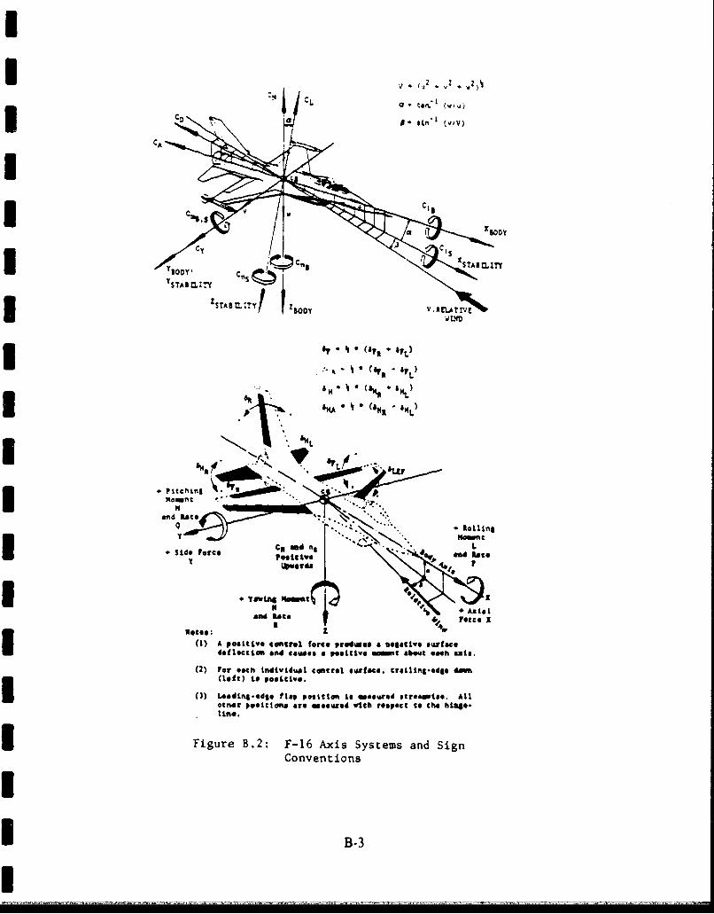
i

I

'

3 Z5y V. CaYIs

"I * (eLAp o e.* v,

-B- C'- " x)

I, NA A E S

IS -i II . "B D' " ',,,;,1,A (&MR. - ....)

I . Side P• . -.t.

pitc nc X

-- Noow :

(1) A poRattve eafItrel forte prmaa a sai ufe__ dafti.. and Ratae. a p"Iitiv. m ~t Tbot te s anie.

(2) For each individual control stface, crailin*-.dej e(left) to posLlive.

(3) L4sding.-dj* flapo poescito to wmasured etreaawit. Alloter postaitma are eaourod with respect to t•e hLgso-line.

Figure B.2: F-16 Axis Systems and Sign

Conventions

B-3

I

Appendix C: Control Derivative Conversion ProgramIThis appendix contains the computer program used to convert the data listed in

3 Appendix A on page A-2 from the stability axis to the body axis. The program was

developed and used in Reference 8. Primed and unprimed dimensional derivatives are

I also calculated ia this program. In addition to values for control derivatives, other

parameters such as aircraft mass moments of inertia, trim conditions, and flight

conditions are also input. Outputs are shown in Appendix A on pages A-3 and A-4.

IIIIIIIIIIII C-1

I

I

PROGRAM CATREAL ALPHA,CL,CLA,CLDE,CLDF,CLQ,CLAD,CLU,

1CD,CDA,CDDE,CDDF,CDU,2CZ,CZA,CZDE,CZDF,CZQ,CZAD,CZU,3CX,CXA,CXDE,CXDF,CXU,DALPHA,DPR,4CNB,CNP,CNR,5CNDR,CNDA,CNDDT,CNDC,6CLB, CLP, CLR,

7CLDR,CLDA,CLDDT,CLOC,SCYP, CYR, L, N,9M,M1,MA,MAD,MQ,MU,MDE,MDF

CHARACTER*3 KEY, KEYl, DATA1, DATA2, DATA3, RUN

DPR - 57.2957795S~WRITE(*,5)

5 FORMAT( lX,' **********''****''*****i***.***.************,*******,)

WRITE(*,10)10 FORMAT(lX,'******** AXIS TRANSFORMATION PROGRAM ***************)

WRITE(*,20)20 FORMAT(1X,'****************************************************I)

WRITE(*,100)100 FORMAT(1X,'ENTER STABILITY AXIS COEFFICIENTS FOR TRANSFORMATION')SkWRiTE(*,101)101 FORMAT(1X,'TO BODY AXIS. TRIM ALPHA IS NEEDED FOR CONVERSION.')

WRITE(*,102)102 FORMAT(lX,'MOMENT COEFFICIENTS AND SIDEFORCE COEFFICIENTS NOT')

WRITE(*,40)40 FORMAT(IX,'REQUESTED REMAIN UNCHANGED.')

WRITE(*,41)41 FORMAT(lX,lNOTE: ALL COEFFICIENTS ARE REQUESTED WHEN COMPUTING')I WRITE(*,42)

42 FORMAT(IX,'DIMENSIONAL DERIVATIVES.')103 CONTINUEWRITE(*,30) S30 FORMAT(1X, '*t************************************.************U,)

WRITE(*,106)106 FORMAT(IX,'TO TRANSFORM ONLY LONGITUDINAL DATA - TYPE LONG')

WRITE(*,107)107 FORMAT(1X,'TO TRANSFORM ONLY LATERAL-DIRECTIONAL DATA - TYPE LAT')

WRITE(*,108)108 FORMAT(IX,ITO TRANSFORM BOTH LONG AND LAT-DIR DATA - TYPE BOTH')WRITE (*, 111)

I 111 FORKAT(IX,'KEYWORD " '

READ(*,109) KEY109 FORMAT(A3)IF(KZY .EQ. 'LAT') 0 TO 104IF(KZY .EQ. 'LON') 0 TO 104IF(KEY .EQ. 'BOT') GO TO 104GO TO 103

104 CONTINUE2000 CONTINUE

WRITE(*,2010)2010 FORMAT(1X,'ARE DIMENSIONAL BODY AXIS DERIVATIVES REQUIRED ? (YES/

1NO)')READ(*,2020) KEY1

2020 FORMAT(A3)WRITE(*,2030)

2030 FORMAT(1X,'***h************ ******************************')IF (KEYI .EQ. 'YES') GO TO 2040IF (KEY1 .EQ. 'NO ') GO TO 2150GO TO 2000

C-2

2040 CONTINUEWRITE (*,2 050)U2050 FORKAT(lX,'Q (DYNAMIC PRESSURE - LBS/FT**2)READ(*,*) QWRITE(*, 2060)

2060 FORMAT(1X,'S (WING REFERENCE AREA - FT**2)READ(*,*)SWRITE(*, 206!)

2065 FORMAT(1X,@C (WING MEAN AERODYNAMIC CORD -FT)

READ(*,*) CI WRITE(*,2070)2070 FORKAT(lX,'B (WING SPAN - FT)

READ(*,*) BWRITE( *,2080)I2080 FORMAT(1X,'VT (TRIM VELOCITY -FT/SEC)

READ (*,*) UWRITE(*,2081)

2081 FORKAT(1X, 'THETA (PITCH ANGLE -DEGS)I READ(*,*) ]>THETAWRITE(',2085)

2085 FORMAT(lX,lW (WEIGHT - LBS)READ(*,*) WU ~WRITE(*, 2090)

2090 FORMAT (1X, 'INERTIAS MUST BE INPUT IN BODY AXIS.')WRITE(*, 2100)

2100 FORMAT(1X,IIXX (SW$G-PI**2) -I READ(*,*) BIXXWRITE(*, 2110)

2110 FORKAT(1X,@IYY (SWJG-FT**2) aREAD(*,*) BIYYI ~WRITE(*, 2120)

2120 FORMAT(1X,'IZZ (SWJG-FT**2) -READ(*,*) BIZZWRITE(*, 2130)I2130 FORMAT(1X,'IXZ (SWJG-FT**2) -READ(*,*) BIXZWRITE(*, 2140)

2140 FORKAT(1X,*O.*****t*****I***********.*WRITE(*, 3030)

3030 FORMAT(16X, $AIRCRAFT PARAMETERS')WRITE(*,3050) Q

3050 FORMAT(1X1'Q (DYNAMIC PRESSURE - LBS/rT**2) a',G13.6)

306 FORKITz(h,0) WN REFERENCE AREA - FT**2) 1 ,G13.6)WRITU(*,3065) C

305TO RMA T(lX,IC (WING MEAN AERODYNAMIC CORD - FT) - 1,G13.6)WRITZ(*,3070) B

3070 FORKAT(1X,13 (WING SPAN - FT) - 1,G13-6)WRITZ(*,3080) U

3080 FORMAT(1X,'VT (TRIM VELOCITY - IT/SEC) - 1,G13.6)WRITE(*,30S1) OTHLETA

3081 FORMAT(1X,ITHETA - 1,G13.6)WRITE(*,3085) W

3085 FOW'IAT(1X, I (WEIGHT - LBS) - ',G13.6)

WUITE(*,3100) BIYY

311 ?ORMAT(1X,OIYY (SWJG-FT**2) - 1,G13.6)WRITE(*,3120) 8122

3120 FORMAT(1X,'IZZ (SWJG-FT**2) - ',G13-6)

3 C-3

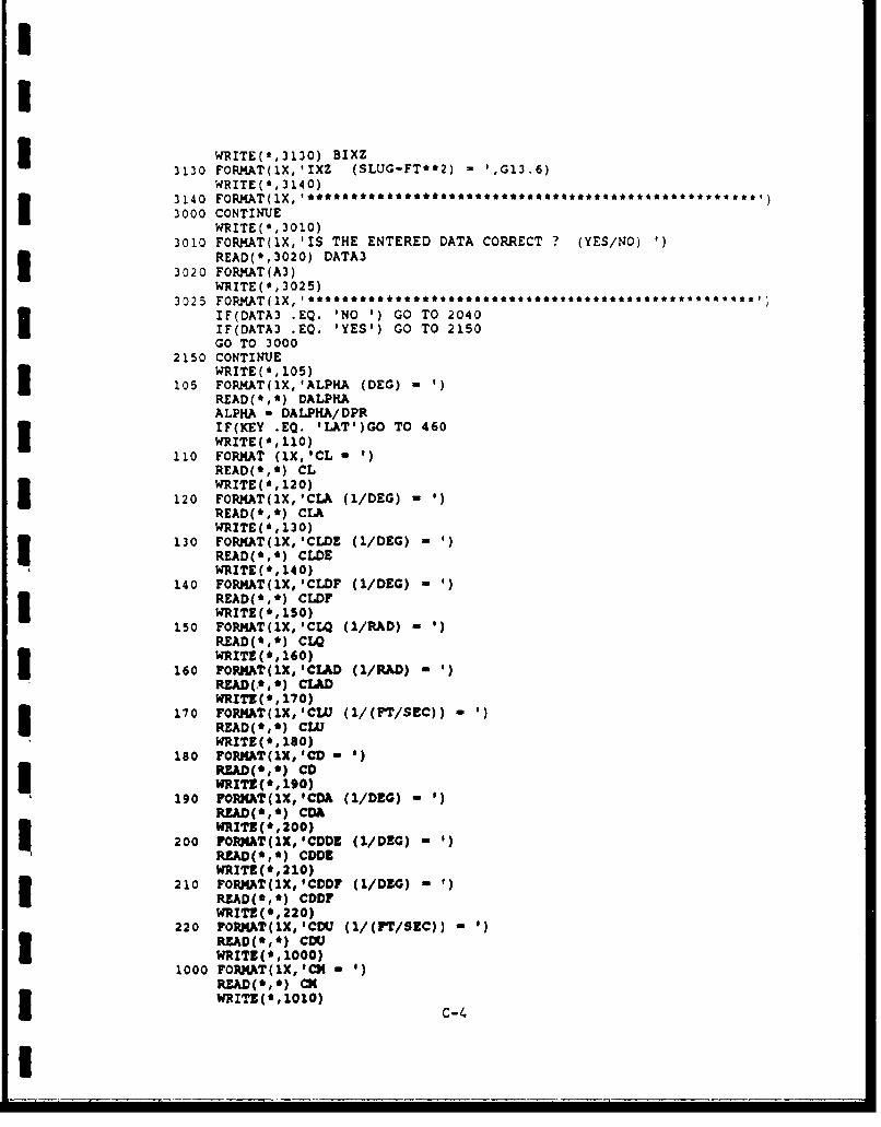
3 WRITE(*,3130) BIXZ3130 FOPMAT(lX,IIXZ (SL.UC-FT**2) '036

WRITE(', 3140)3140FOAT1,**************************'

3000 CONTINUEWRITE( i,3010)

3010 FORI4AT(1X, 'IS THE ENTERED DATA CORRECT ? (YES/NO) *

READ(*,3020) DATA3I3020 FORMAT(A3)WRITE(', 3025)

3025 RMT1,'IIF(DATA3 -EQ. 'NO 1) GO TO 2040I ~IF(DATA3 .EQ. 'YES') GO TO 2150GO TO 3000

2150 CONTINUEWRITE(', 105)

105 FORMAT(lX,IALPHA (DEG)READ(*,*) DALPHAALPHA - DALPHA/DPRIF(KEY .EQ. 'LAT')GO TO 460

110 FORKAT (1X,'CL WIE'10READ(*,*) CLWRITE(*,120)I 120 FORHAT(lX,'CLA (1/DEG)-READ(*,*) CLAWRITE(*,130)

130 FORMAT(1X,#CLDE (1/DEG)-READ(*,*) CLDEWRITE(*,140)

140 FORMAT(1X,'CLDF (1/DEG) -)

READ(*, *) CLD)F

150 FORKAT(1X, 'CL40 (1/RAD) WXE'10READ(*,*) CWQWRITE ', 160)

160 FORMATI'(X, OCID (1/RAD)-READ(.*,') CLAD

WRITZ(',170)170 FORKAT(1X,'CW (1/(F¶'/SEC))-

READ(*, ) CWJ

180 -*180

18 ORXAT(lX,'CD- (1/G)-READ(*,) CDWRITZ(*, 200)

200 1'ORMAT(lX,'CDDE (I/DEG) - 1READ(*,*) CDDEWRITE(*,2 10)

210 FORMAT(1X,'CDD? (I/DEG) - 1I READ(*,*) CDDFWRITE(*, 220)

220 FORMAT(1X,'CDOI (1/(VT/S-C))READ(*,*) CDUrWRITE(*,2100)

1000 FORMAT(1X,ICU(1/- I) C)

READ(*,*) 04UWRITZ(',1010)

WRIT (*,1 10)C-4

1010 FOR.MAT(1X,'CMA (1DEG)READ(*,*) CMAIF (KEY1 .EQ. 'NO ') GO TO 1005WRITE(*, 1030)

1030 FORMAT(1X,'CMDE (1/DEG) -READ(*,*) CMDEWRITE(*, 1040)

1040 FORMAT(lX,'CMDF (I/DEG) -READ(*,*) CMDF

105 FOKAos:'M (1/RAD)READ(*,*) CMQ

105CONTINUEWRITE(*, 1060)

1060 FORMAT(1XCKAD (1/R.AD) 1)READ(*,*) CMADWRITE(*, 1020)I 1020 FORMAT(lX,'CNU (1/(FT/SEC))-READ(*,*) CMUWRITE(*, 225)

225WRITE(*, 226)

226 FORMAT(6X, 'LONGITUDINAL STABILITY AXIS COEFFICIENTS')WRITE(*,230) DALPHAI230 FORMAT(15X,'ALPKA -1,G13.6)IF (KEY1 -EQ. 'YES') GO TO 1080WRITE(*,240) CL,CD

240 FORMAT(lX,'CL - ',G13.6,6X, 'CD - I G13.6)WRITE(*,250) CLA,CDA

250 FORMAT(lX,'CLA - ',Gl3.6,5X,'CDA - ,G13.6)WRITE(',260) CLDE,CDDE

260 FORMAT(lX,'CLDE - ',G13.6,4X,'CDDE - 1,G13.6)WRITE(*,270) CLDFCDDF

270 FORMAT(lX, CLDF - 1,G13.6g4X, lCDOF - 1,G13.6)WRITE(*,280) CLQ

280 FORMAT(1X,'CLQ - 0,G13.6)WRITE(*,290) CLAD

290 FORNAT(1X,'CLAD - ',G13.6)W'RITE(*,300) CWFJCDU

300 FORMAT(MICWU 1 ,Gl3.6,SX,'CDU - ,G13.6)1080 CONTINUE

IF(KEY1 .EQ. 'NO 1) GO TO 1170WRIZT(*,1090) CLCM,CD

1090 FORNAT(4X,'CL - ',Gl3.6,9X,cXl - 1,G13.6,6X,'CD - ,G13.6)I. VRITE(*, 1100) CIA,OIACD&1100 FOR3EAT(3X,'CLA - ',G13.6,lX,'O(& - 1,Gl3.6,:X,'CDA - ',G13.6)

WRITZ(*,1110) CWDE,O4DE,CDDE1110 ?ORNAT(2X,ICLOE - 1,G13.6,7X,ICMDZ - f,Gl3.6,4X,lCDDZ - 1,G13.6)I WRITS(*1 1120) CLDF,OXDF,CDDY1120 FORMAT(2X,*CLDF - ',G13.6,7X,'CNDF - ',Gl3.6,4X,ICDDF - 1,G13.6)

WRITE(*,1130) CLQ,CMQ1130 FORMAT(3X,'CLQ - 1,Gl3.6,SX,'CMQ - 1,G13.6)I VRITE(*,1150) CLAD,CMAD1150 FORMAT(2X,'CIAD - 1,G13.6,7X,ICMAD - 1,G13.6)

WRITE(*, 1140) CLUC(U,CDU1140 FORMAT(3X,ICWU - ,Gl3.6,SX,'04U - 1,Gl3.6,SX,'CDU - ,G13.6)1170 CONTINUE

WRITE(*, 310)310 FRA(X ********i********i********'

I315 CONTINUE C-5

WRITE(*,320)I320 FORM4AT(1X, ' IS THE ENTERED DATA CORRECT ? (YES./NO) 6)

READ(',330) DATA3.330 FORMAT(A3)

WRITE(*,335)I ~ ~~~335 OMT X:*********** **** ***** )

IF(DATA1 .EQ. 'YES') GO TO 3450IFDT1E.@E' OT 4GO TO 315

340 CONTINUEWRITE (*, 3 45)1345 FoRMAT(6,'ILONGITUDINAL BODY AXIS COEFFICIENTS (1/RAD)I)

CLA - CLA*DPRCLDE - CLDE*DPRCLDF - CLDF*DPRCDA - CDA*OPRCDDE -CDDE*DPR,CDDF - CDDF*DPRCMA a CMA*DPRI C IF (KEY1 .EQ. 'NO ')GO TO 346

CCMDE -CIIDZ*DPRCNDF -CMDF*DPR

346 CONTINUEC

SCZA - -CLJA - CD* SCZAD -- CLAD

SCZQ -- CLQ

SCZDZ - -CLDE .0CSCZDF - -CLDF

SCXA - -CDA + CLSCXU - -CDU - 2.O*CDSCXDZ a -CDDISCXDF - -CDDF

CCAL - COS(ALPHA)SAL - SIN(ALPHA)COSSQ a CAL**2SINSQ - SAL**2COSSIN - CAL'SALI C CZ w -CL*CAL - CD*8ALCZA - SCZA*CO8SQ + (SCZU+SCXA) *COSS IN + SCXU*SIIISQCZAD - SCZAD'COSSQI CZQ - SCZQ*CALCZU - SCZU'COSSQ - (SCZA-SCXU) *COSSIN -SCXA*SINSQ

CZDZ - SCZDE'CAL + SCXDZ*SALCZDF - SCZD?*CAL + SCXDF*SALI C CX - -CD*CAL + CL*SALCXA - SCXA*COSSQ + (SCXU-SCZA) *COSSIIE SCZU*SINSQCXAD - CTJ.D*COSSINI CXQ - CLQ'UALCXU - SCXU*COSSQ - (SCXA+SCZU) *COSS IN + SCZA*SINSQCXDE - SCXDE*CAL - SCZDE*SAL3 CXDF - SCXDF'CAL - SCZDF'SAL

c-6

I ~BCMA - CKA*CAL + (CM1U + 2.0*CM)*SALBCMAD -CKAD*CAL3BCMU -(CMU + 2.0O*CM) *CAL - CMA*SAL

WRITE(*,350) CZ,CX350 FORMAT(4X,'CZ - ',Gl3.6,33X,'CX -',G13.6)

WRITE(*,360) CZA,BCMA,CXA360 F0RJMAT(3X,'CZA - @,G13.6,8X,'CMA -',Gl3.6,5X,'CXA -',G13.6)

WRITE(*,370) CZDE,CXDE370 FORMAT(2X,'CZDE a 1,G13.6,31X,'CXDE a 1,G13.6)

IJRITE(*,380) CZDF,CXDF380 FORMAT(2X,'CZDF - ',Gl3.6,31X,'CXDF = ',G13.6)

1'RITE(*,390) CZQ,CXQ390 FORMAT(3X,'CZQ - ',Gl3.6,32X,'CXQ - ,G13.6)

WRITE(*,400) CZAD,BCMAD,CXADI400 FORMAT(2X,'CZAD - ',G13.6,7X,ICMAD - ',G13.6,4X,ICXAD = ,G13.6)WRITE(*,410) CZU,BCMU,CXU

410 FORMAT(3X,'CZU - ',G13.6,8X,'CMU a',Gl3.6,SX,'CXU -',G13.6)IJRITE(*, 420)

420 FORMAT(lX, ******t*******************)IF (KEY1 -EQ. 'NO I) GO TO 1360Zi (Q*S*32.2)/WA -C/(2.0*U)

THETA - DTHETA/DPR

Z aQ*S*CZZA aZl*CZAI ZAD - Zl*A*CZADZQ - Z1*A*CZQZU (Z1/U)*CZUZDE - Z1*CZDEZDF a Zl*CZDF

a Q*S*CXXA- Z1*CXA

XAD a Zl*A*CXAD

XDE - Zl*A*CXQ

C

MAD a M1**A'/BCHA

MQ a M12*A*CMQMUt am (M1/U)*BQIMDE a M1*QED3MD? -a Ml'CIDF

CI ~WRITZ(*, 1100)1180 FORMAT (SX, 'LONGITUIDINAL AXIS DIMENSIONAL DERIVATIVES-)

WRITZ(*,1190) Z,M,X1190 FORMAT(SX, 'Z an ',G13.6, 10X,M IN ',G13.6,7X,'IX - ',G13.6)U VRITZ(*,1200) ZA,MA,Xk1200 FORMAT(4X,IZA a 1,G13.6,9X,'f(KA ',G13.6,6X,'XA a I,G13.6)

WRITE(*,1210) ZDE,MDE,XDI1 1210 FORI4AT(3X,'ZDZ - ',Gl3.6,SX,'MDE - ',G13.6,SX,IXDE - ',G13.6)

c-7

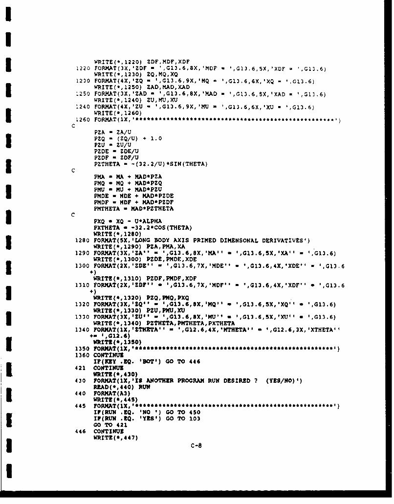
WRITE(*,1220) ZDF,MOF,XDF

1220 FORKAT(3X,'ZDF - ',Gl3.6,8X,'MDF~ a ',G13.6,5X,'XDF - ,G13.6)WRITE(',1230) ZQ,MQ,XQ

1230 FORMAT(4X,'ZQ - ,G13.6,9X,'MQ - ',Gl3.6,6X,'XQ - ',G13-6)WRITE(',1250) ZAD,M.AD,XADI1250 FOR1MAT(3X,'ZAD - ',Gl3.6,SX,'?QAD = 1,G13.6,5X,'XAD = ',G13.6)WRITE(',1240) ZU,MU,XU

1240 FORMAT(4X,'ZU - ',G13.6,9X,'MU ',Gl3.6,6X,'XtJ ',G13.6)WRITE(', 1260)I ~ ~~~1260 OMT1,'*****************h*******)

PZA - ZA/UPZQ - (ZQ/U) + 1.0I ~PZLJ - ZtJ/UPZDE - ZDE/UPZDF n ZDF/UPZTHETA - -(32.2/U)*SIN(THETA)

PMA - MA +. MAD*PZAPMQ - MQ + MAD*PZQPMU - MU + MAD*PZUI PMDE - MDE + MAD*PZDEPMDF - MDF + MAD*PZDFPMTHETA - MAD*PZTHETA

I PXQ - XQ - U*ALPHAPXTHETA - -32.2*COS(THETA)WIRITE(*, 1280)

1280 FORMAT (SX, ILoONG BODY AXIS PRIMED DIMENSONAL DERIVATIVES')I IJRITE(*,1290) PZA,PMA,XA1290 FORMAT(3X,1 ZA'' - 1,G13.6,8X,'MA'' a ',G13.6,5XIXA'' - ',G13.6)

WRITE(*, 1300) PZDE,PMDE,XDE1300 FORMAT(2X,'ZDE'' - ',G13.6,7X,'MDE'' - 1,G13.6,4X,IXDE'' -',G13.6

+.)

WRITE(*,1310) PZDFPMDF,XDF1310 FORMAT(2X,IZDF'' - ',G13.6,7X,-MDF"' - ',G13.6,4X,'XDF'' 1 ,G13.6

I WRITE(*,1320) PZQ,PMQ0,PXQ1320 FORMAT(3X,'ZQ'' - l,G13.6,SX,lMQl' - ',G13.6,5X,'XQ'' - 1,G13.6)

WRITE(',1330) PZUPMUXU1330 FORMAT(3X,#ZU'' - ',G13.6,8X, 'MU'' - ',G13.6,5X,'XUl' a 1,G13.6)I ~ ~WRITE (*, 1340) PZTHETA, PM'THETA, PXTHETA1340 F0RNAT(1X,'ZTHZTA'' - ',Gl2.6,4X'lMTHETA'' a ,G12.6,3X,lXTHETAl'

+- ,G12.6)WRITR(*, 1350)I ~ ~~~~1350 FORMAT(1X,'**************************)

1360 CONTINUEIF(KEY .ZQ. #DOT#) GO TO 446

421 CONTINUEVRITE(*, 430)

430 TORMAT(IX,'IS ANOTHER PROGRAM RUN DESIRED 7(YES/NO)')READ(*,440) RUN

440 FORMAT(A3)WRITE (*,445)

445 FRA(X ******************t*******'

IF(RUN .EQ. 'NO ') GO TO 450IP(RUN EKQ. 'YZS') GO TO 103I GO TO 421

446 CONTINUEWRITE(*,447)3 C-8

447 FOR.MtAT(1X, ********************t*a**)

460 CONTINUEWRITE(*,455)

455 FOR.MAT(lX,'CNB (1/DEG) aREAD(*,*) CNBWRITE(*,470)

470 FORJMAT(lX, 'CNP (1/RAD) mREAD(*,*) CNP

480 F0RMAT(lX, 'CR (1/RAD) n TE1)80READ(*,*) CNRWRITE (*,490)

490 FORMAT(lX, 'CNJDR (1/DEG) -READ(*,*) CNDRWRITE(*,500)

500 FORMAT(lX, 'CNDA (I/DEG) - 0

READ(*,*) C?4DAWRITE(*, 510)

510 FORKAT(1X, 'CNDDT (I/DEG)READ(*,*) CNDD`T

520 FORMAT(1Xg*CNDC (1/DEG) RT(,50READ(*,*) CNDCWRITE(',530)

530 FORMAT(lX,'CLB (1/DEG) -

WRTEA(*,*54) C :;: :WRITE(*, 550)

READ(*,*) CLRWRITE(*, 560)

560 FORMAT(1X,ICLDR (1/RDI) - 1)READ(*,*) CLORWRITE(*, 570)I!570 FORKAT(1X,ICLDA (1/DIG) -READ(*,*) CLD&WRITE('. 560)

580 FORMAT(1XICLDDT (1/DIG) -READ(*,*) CLODAI: VRITZ(', 590)

590 FORKAT(1X,tCLDCT (1/DIG) 1)READ(*,*) CLOCT

611 FORMAT(1X,ICYB (I/DEG) OnREAD(b, *) CLXI

VIF (*P~ 600) ($/RAD) GO TO60I' WRITI(*, 610)61FOPJIAT(1X,ICYS (1/ADE)

READ(*,*) CYS

612 FORI4AT(lX,'CYDR (1/RDI) WRT(*62READ(*,*) CYDR

WRITZ(',613)

61IOMTI,#Y 1RD

613 FORMAT(lX,'CYDA (I/DEC)READ(*,*) CYDAWRITE (*,614)

614 FORMKAT(lX,'CYDDT (1/DEG)READ(*,*) CYDDTWRITE(*,615) (/DG

READ(*,*) CYDC66CONTINUEI WRITE(*,620)

620 FRA(X ***************,,**,******

WRITE(*, 630)630 FOR.MAT(SX,'LAT-DIR STABILITY AXIS COEFFICIENTS-)I ~IF(KEY .EQ. 'LON') GO TO 635

IF(KEY .EQ. 'BOT') GO TO 635WRITE(*,631) DALPHA

631 FORMAT(15X,'ALPHA - 1,G13.6)I635 CONTINUEIF(KEY1 .EQ. 'YES') GO TO 711WRITE(*,640) CNB,CLB

640 FORMAT(3X,'CNB - ',G13.6,SX,'CLB - ',G13.6)I WRITE(*,650) CNP,CLP,CYP650 FORMAT(3X,'CNP - ',G13.6,8X,lCLP - ',Gl3.6,5X,'CYP a 1,G13.6)

WRITE(',660) CNR,CLR,CYR660 FORMAT(3X,'CNR - ',Gl3.6,SX,'CLR - 1,G13.6,5X,ICYR - 1,G13.6)I WRITE(*,670) CNDR,CLDR670 FORMAT(2X,'CNDR - 1,Gl3.6,7X,'CLDR - ',G13.6)

WRITE(*,680) CNDA,CLDA680 FORMAT(2X,'CNDA - 1,G13.6,7X,'CLDA - 1,G13.6)I ~WRITE (*,690) CNDDT, CLDDT690 FORMAT(lX,IC?40DT - 1,G13.6,6X,ICLDDT - 1,G13.6)

WRITE(*,700) CNDC,CLDC700 FOPMAT(2XDCNDC - ',Gl3.6,7XICLDC - ',G13.6)I WRITE(*,710)710 FRA(X **************************'

IF(ICEY1 .EQ. 'NO ') GO TO 720711 CONTINUEI'WRITE(*,712) CLY712 FORNAT(3X,'CNB - 1,G13.6,SX,lCLB - ',Gl3.6,SX,ICYB - ',G13.6)

WRITE(*,713) CNPCLPgCYPI713 FORMAT(3X,'CNP - ',Gl3.6,SX,'CLP - ',Gl3.6,5X,'CYP - 1,G13.6)WRITE(*,714) CNR,CLR,CYR

714 FORJ(AT(3X,'OfR - ',Gl3.6,SX,'CLR - 1,G13.6,5XICYR - 1,G13.6)WRITZ(',715) CHDR,CWDR,CYDRI 715 FORIEAT(2X,'CNDR - 1,G13.6,7X,ICLDR - 1,G13.6,4X,ICYDR - ',G13.6)WRITI(',716) CIIDA,CLDA,CYDA

716 FORJ(AT(2X,OIDA - ',Gl3.6,7X,lCLDA - 1,G13.6,4X,ICYDA - 1,G13.6)WRIT! (*,717) CNDDT,CLDD>T, CYDDT

717 FORNAT(lX,ICNDDT - 1,Gl3.6,6X,ICLDD>T - '1 G13.6g3X,'CYDDT - 1,G13.6in:. +)WRITE(*,718) CNDC,CLDC,CYDC

718 FORKAT(2X,'CNDC - 1,G13.6,7X,'CLDC - ',Gl3.6,4X,'CYDC 1 ,G13-6)I WRITE(*,719)719 FRA(X **************************'720 CONTINUE

WRITZ(*,730)I730 ?ORMAT(lX,'IS THE ENTERED DATA CORRECT ? (YES/NO)')READ(*,740) DATA2

740 FORMAT(A3)WRITZ(*,750)c-

I-1

I ~IF(KEY .EQ. 'BOT-) GO TO 755IF(DATA2 .EQ. 'NO ') GO TO 2150IF(DATA2 .EQ. 'YES') GO TO 760GO TO 720I755 CONTINUEIF(DATA2 .EQ. 'NO ') GO TO 460IF(DATA2 .EQ. 'YES-) GO TO 760GO TO 720

760 CONTINUECNB-CNB*DPRCNDR-CNDR* DPRCNDA -CNDA*DPRCNDDT-CNDDT*DPRCNDC-CN DC'DPRCLB-CLB' DPRCLDR-CLDR* DPRCLDA-CLOA' DPRCLDDT-CLDDT' DPRCLDC-CLDC' DPRIF(KEY1 -EQ. 'NO ') GO TO 765CYB *CYB*DPRCYDR -CYDR*DPRCYDA -CYDA*DPRCYDOT -CYDDT*DPR

I765 CNIUBCLB - CLB*COS(ALPHA)-CNB*SIN(ALPHA)BCLP-CLP*COS (ALPHA) **2- (CLR+CNP) *SIN (ALPHA) *COS (ALPHA) +CNR*S IN (ALP

BCLR-CLR.COS (ALPHA) **2-(CNR-CLP) *SIN (ALPHA) *COS (ALPHA) -N* N(LI. BCLDA - CLDA*COS (ALPHA) -CI4DA*SIN (ALPHA)BCLDR - CLDR*COS (ALPHA) -CNDR*SIN (ALPHA)BCLDC - CLDC*COS (ALPHA) -CNDC*SIN (ALPHA)BCLDDT - CLDDT*COS (ALPHA) -CNDDT*SIN (ALPHA)I. ~BCNB - CNB'COS (ALPHA) +CLB*SIN (ALPHA)BCNP - CNP*COS (ALPHA) **2- (OrR-CLP) *SIN (ALPHA) *COS (ALPHA) -CLR*SIN (A

lLPHA) '*2BCWR - CNR*COS (ALPHA) **2* (CLR+CIP) *SIN (ALPHA) *COS (ALPHA) +CLP*SIN (AI 1lLPHA) '*2BCNDA - CHDA *COS (ALPHA) +CLDA*S IN (ALPHA)

BCNDR - CNDR*COS (ALPHA) 4CLDR*SIN (ALPHA)BCNDC - CNDC*COS (ALPHA) +CLDC*SItI (ALPHA)I. BCHDD'r - CNDDT'COS (ALPHA) +CWDDT*SIN(ALPIIA)BCYR - CYR*COS (ALPHA) +CYP*SIN (ALPHA)SCYP - CYP'COS (ALPHA) -CYR*SIN (ALPHA)WRITE(*,770)I'770 FORMAT (9X, 'LAT-DIR BODY AXIS COEFFICIENTS')WRITE(*,780) BCNBgDCLBCYS

780 FORI4AT(3X,'CND - l,G13.6,SX "'CLB - ',Gl3.6,SX'ICYB - ',G13.6)WRITE(*,790) BCNP,BCLP,9CYP

790 FORMAT(3X,'CNP - ',G13.6,9X "'CLP - ',G13.6,5SX,'CYP - ',G13.6)WRITE(*,S0O) BCNR,BCLRt,BCYR

800 FORMAT(3X,'CNR - 1,G13.6,$X .'CLR - ',G13.6..5X,ICYR -',G13.6)

WRITE(t,810) SCWDR,BCLDR,CYDR810 FORMAT(2X,'ICNDR a 0,Gl3.6,7X, CLDR a 1,G13.6,4X, 'CYDR - 1,G13.6)

WRITE(*,820) BCNDA,BCLDA,CYDA

820 FORMAT(2X,'CI4DA - ',G13.6,7X,'CLDA a ',G13.6,4X,'CYDA - ',G13.6)3 ~WRITE(*,830) BCNDDT,BCLDDT1,CYDDT

C-11I

330 FORMIAT( IX, 'CN DDT 'G13.6, 6X, CLDDT 'G13. 6,3X, 'CYC-DT = ,:13. 6

W-RITE(*,840) BCNDC,BCL.DC,CYDC840 FORMAT(2X,'CNDC - ',G13.6,7X,'CLDC 1,G313.6,4X,ICYDC ',G!3.6)

wMrTE(',B 50)

IF (KEY1 .EQ. 'NO ')GO TO 421

N - (Q*S*B)/BIZZL - (Q*S*B)/BIXX

B=B/(2.0*U)Y-(Q*S*32.2)/W

BNB - N*BCNB8NP - N*B*BCNPI BNR - ?4*B*BCNRBNDR - N*BCNDRBNDA = N*BCNDABNDDT - N*BCNDDTBNDC = N*BCNDCBLB a L*BCLB

BLP a L*B*BCLPBLR - L*B*BCLRBLDR - L*BCLDRBLDA - L*BCLDA

BLDDT - L*BCLDDTBLDC - L*BCLDCI YB -Y*CYBBYR - Y*B*BCYRBYP - Y*B*BCYPYDR - Y*CYDRI 'iDA - Y*CYDAYDDT a Y*CYDDTYDC a Y*CYDCWRITE(*,2160)I2160 FORMAT(SX,ILAT-DIR BODY AXIS DIHENSIONAL DERIVATIVES')wRITE(*,2170) BNB,BLBYB

2170 FORMAT(4X,'NB - ,Gl3.6,9X,ILB = ',Gl3.6,5X,'YB - 1,G13.6)WRITE(*,2180) BNP,BLP,BYPI2180 FORHAT(4X,INP a '1 Gl3.6,9X,'LP a 1,Gl3.6,5X,IYP a 1,G13.6)WRITE(*,2190) BXR,BLR,BYR,

2190 FORMAT(4X,'NR- a ,Gl3.6,9X,'LtR a ',Gl3.6,5X,'YR a ',G13.6)IJRITE(*,2200) BNDR,BLDR,YDRI 2200 FORI(AT(3X,'NDR a 1,Gl3.6,8X,'LDR a ',Gl3.6,4X,'YDR = ',G13.6)WRITE(*,2210) BNDA,BLDA,YDA

2210 FORMAT(3X,INDA a 1,G13.6,8X,'LDA a 1,Gl3.6,4X,'YDA a IG13.6)WRITZ(*,2220) BNDDT,BLDDT,YDDTI2220 FORMAT(2X,'NDI>T a 1,G13.6,7X,ILDDT a ',Gl3.6,3X,IYDDT a 1,G13.6)WRITE(*,2230) BI4DC,BLDC,YDC

2230 FORKAT(3X,INDC a 1,G13.6,8X,ILDC a 1,G13.6,4X,IYDC - ',G13.6)WRITE(*, 2240)I ~ ~~~2240 FRA(X .. ****.********..*******t*'

D a1.0 - ((BIXZ*BIXZ)/(BIXX*BIZZ))Rl BIXZ/BIZZR2 -BIXZ/BIXXI PBMB a (BNB + Rl*BLB)/DPBNP a (SNP + R1*SLP)/DPBN2R a (BNR + Rl*BLR)/DPBNDR a (BNDR + Rl*BLDR)/DI PBNDA - (BNDA + Rl*BLDA)/DPBNDDT a (BNDD`T + Rl*BLDDT)/DPBNDC a (BNDC + Rl'BLDC)/D

C-1 2

PBL.B - (BL.B +R2*BNB)/DPBLP - (BLP + R2*BNP)/DPBLR -(BLR + R2*BNR)/DPBLDR - (BLDR + R2*BNDR)/DPBLDA -(BLDA + R2*BNDA)/DPBLDDT - (BLDDT + R2*BNDDT)/DPBLDC a(BLDC + R2*BNDC)!DPYB -YB/UPSYP *BYP/U + ALPHA

PBR BYR/U - 1.0PYOR -YDR/U

PYDC D/

PYC YDC/UWRITE(*, 2250)

2250 FORKAT(3X,J.AT-DIR BODYt AXIS PRIMED DIMENSIONAL DERIVATIVES-)I WRITE(*,2260) PBNB,PBLBPYB2260 FORMAT(3X,'NB'' - ',G13.6,SX,'LB'' - ,Gl3.6,4X,'YB'' - ',G13.6)

WRITE(*,2270) PBNP,PBLP,PSYP2270 FORMAT(3X,'NP'' - ',G13.6,8X,'LP'' - ',Gl3.6,4X,IYP'l - ',G13.6)I ~WRITE(*,2280) PBN4R,PBLR,PBYR2280 FORMAT(3X,@NR" - ',Gl3.6,$X,ILRI' - 1,Gl3.6,4X,IYR'' - ',G13.6)

WRITE(*,2290) PBNDR,PBLDR,PYDR2290 FORKAT(2X,@NDR'' - ',Gl3.6,7X,'LDR'' - ',Gl3.6,3X,'YDR'' = ',G13.6I 4)WRITE(*,2300) PBNDA,PBLDA,PYDA2300 FORKAT(2X,'NDA'' - ',Gl3.6,7X,'LDA' - ',Gl3.6,3X,IYDA'' - ',G13.6I. WRITE(*,2310) PBNDDITPBLDDIT,PYDDT2310 FORMAI'(2X,'NDDT'' - ',G13.6,6X,'LDDT''- ',Gl3.6,2X,'YDDT'' - 1,Gl

*.6)WRITE(*,2320) PBNDC,PBLDCPYDC

2320 FORMAT(2X,'NDC'' - ,G13.6,7X,ILDC'' -,Gl3.6,3X,IYDC'' 1 ,Gl1J.6

2340

END

CI1

Il

Appendix D: Linearized Equations of Motion

The linearized equations of motion derived in this appendix are used to create the

state-space system for the F-16. It should be duly noted that this section was taken ver-

batim out of Appendix B of Reference 8. Derivations are made for both primed and

unprimed dimensional derivatives for the three force and three moment equations. The

linearization process is carried out for a specific set of steady-state conditions and is

generally valid for small perturbations about this condition. For this study, the condi-

tions selected about which to linearize the equations of motion for the F-16 were 0.6

Mach number at sea level. Data for this condition are given in Appendix A.

D-I

I1

Aircraft Equations of Motion

Longitudinal Equations - Body Axes

F Fzcg m (W + pV - qU) - mg cose coso (B-1)icg

thus

zcSg _ pV + qU + g cose cost (B-2)

W " i÷ Czaa + (C & + Czqq) c z;+ c

+ Cz6e + Czdf]f (B-3)ISubstituting Eq. (B-3) into (B-2) gives:

~~6U

SCz seo Cz•61 - pV+ qU +g cs os# (B-4)

To develop perturbation equations, a Ig wings level

trim flight condition is examined where *=-0 . ,O , qO ,

1 .3f-0 , AU-0 , p-O , and cosO is approximately one. The trim

3, angle of attack and elevator position are aT and S*T respec-

tively.

I-!• . D-2

I:I --

Ii o L6e + (B-5)

Thus, the aerodynamic forces balance the vehicle's

I weight. To account for small variations from this trim con-

dition, perturbation angle of attack ap and elevator posi-

Ition dep are added to the equation. A term for small changes

in sensed g is also included.

m"[Cs z + Cz(c + + C (6eT + 6ep)]

+ g - (g singT)e (B-6)

Cancelling the terms that are equal from Eq. (B-5)

yields:

US 4Caap + CZ5 .Sep11 - (g "ineT)e (B-7)

The equation is expanded to include perturbations in &, q,

U and 6f by referring to Eq. (B-4).

M+ C q) +C + C doU

+ C.Z61 + q- (g sinOT)O (B-8)

The p subscript Is dropped and. U-VT. AU is expressed as

u. Thus, the perturbation equation is:

D-3

S- ('--)Cz + (g2Ucz& + (_,)Czq + u+ ( +S.)C 6e q + )C 2 q U

eMe + ) CS) f + qU - (g sineT)e (B-9)

or

w CL(Za + (Za)a + (Zq)q + (Z du + (Z,,)6e

+ (Z6 f)6f + qU - (g silneT)e (B-10)w

Dividing by U, letting I - , and gathering the a terms

on the left-hand side of the equation gives:

Z• Zu ,Z6."!(-'&) a (!)a + (--U)q + (-u)u + ,.-U-.e

Sg sinefT+ (-V)6f + q - (-u-- -) (B-11)

I is very small and is ignored. Using the primed

notation and noting that all states are perturbations from

the trim condition, the equation can be expressed as:

Sm(Z)a + (Zq')q + (Z u)u.+ (Z so)SO

+ (z 6 .')6f + (Z8')8 (B-12)

z

' hee a"""" a (B-13)

woe zu-, - SS uI Z + z I + C (8-14)

t Z u n Cs

D-4

U

6e Z8 v- .1JIt C (B-16)

"" (B-17)rn-U mu z6 f

J* ze r.sine 3-8U TIn a similar manner, the force equation in the x-axis is

U reduced to a perturbation equation.

F m(U + qW - rV) + mg sinO (e-19)

5 thus

U-F- - qW + rV-t sine (B-20)

I x AU

0K AS+C +( ~x q 'T uVT

+ Cx6e6e + CxSf6 (B-21)

I IS, c +(C q) C + 6M XO Xe ]q 1T J

i+ Cx + so + C -j qW + rV - sine (B-22)

5 For trimmed flight, thrust exactly equals the drag

3 forces.

T ÷S [C +C aT+ Cz 6e6T] (B-23)

3 Do-C5 a

I °.

The perturbation equation is:

"""LmS C a + Cxq + S Cu + L C6e

L •6f - qW + rV - (g coseT)e (B-24)M xf e

W VBy letting •T = and 8 • , the equation can be

written as:

S- (X) + (Xq)q + (Xu)U + (X e)6e + (X 6 f)6f

- qcTU + rBU + X89 (B-25)

Assuming only longitudinal motion, B and r are zero

and noting that all states are perturbations from trim con-

ditions, the equation is expressed as:

(Xa ')a + (Xu )u + (Xso)60 + (X 6af)6f

+ (Iq )q + (Xe')O (B-26)

where XZa "4 M =c Ca (B-27)M G

XU a _S (B-28)xu as = = C Xu

"x**X * C (B-29)

I 0 uXC (B-30)

IDID-6

Ii

I X T -M -UM S C UQ? (B-31)

X6 X e - -g coseT (B-32)

The pitching moment equation is used to develop the perturb-

ation q equation.

M - 1 lY + pr(Ixx - Izz) - (r 2 - 2)Ixz (B-33)

SIyy - My7 - pr(Ix. - I zz) + (r 2 - p2)Ixz (B-34)

For longitudinal motion only, r and p are zero and the

equation becomes:

" yy

I:I an d

- sc [ 3 + C 0 + (C a + Cq) T

+.+ (5-36' mu VTT + CM eso + CM 61 (B-36)~UT ~606

SIn trimmed flight, the moments are assumed to be zero.

I Mn 4Sc [CM +C% OT+CM eTIaO (337)

- Lotting VT - U , Introducing perturbation angle of attack

5 and elevator position variables, and cancelling the above

D-7

I

U . terms that add to zero, gives the perturbation equation:

M- Sc [Cma + (Cm& + c q) -S + C U

U+ Cmde6e + C M6af] (B-38)

Substituting Eq. (B-38) into (B-35)

3scC I +U 2U Cq + LC cAUI yy my % 2UI yy q yy

P --&c -Sc 6e +-so cm 61 (B-39)yy 6. yy 61

I In dimensional form, this is written as follows:

3 q " (a )a + (M•)• + (Mq )q + (MU)AU

+ (M6e)6e + (Maf)6f (B-40)

Substituting Eq (B-12) for & into Eq. (B-40) and letting AU

be represented by perturbation u yields:

q. -(Mut + MeZa')Q + (Mq + Mq M .)q + (*Mu + (8-Zu4)u

+ (M* + M+ZV6 )60 + (M 6f + Mazat)W

3 (M&Ze")e (B-41)

Using the primed notation, the equation is represented as:

34 (MeIP)a +÷ (Mq')q + (Mu0)U + (u 6e')8e

+ (M6 f')6f + (M .)e (B-42)

D-8

U _i___iI

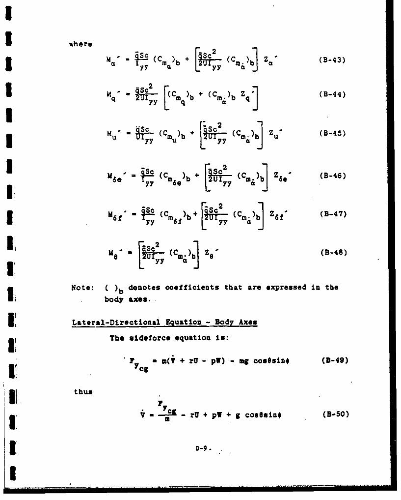
I wheres-c(C )b (Cm) (I (B-43)

"q 2U mq)b + (Cm)b Z

ALu c ( Sc (Cm• Z (B-45)IU LuUy 7 MU)b + 77

"")b" + (dc z (B-46)

Se- (Cm )Y b] r62I: yy e 2 T (CU~ Ze-(-47)

I"f" F - (Cm )b+ (Cm) ZSf" (B47)

L 07Y [2 19t )

2 Iyy (CJ%) Z(B

Note: )b denotes coefficients that are expressed in the

El body axes.

I Lateral-Directional Equation - Body Axes

I! The sideforce equation is:

"Fy m(V + rU - p1) - mg cosOsin# (B-49)

thbusF

I__- rU + p1 + g cos.sin, (B-5o)

3 ~D-9.|I _ _ _ _ _ _ _ _ _

A- a + C + C )b +CIF[CB+ CypPCrr} +CF

M m {0 Y p YT ÷ a.

+ Cy6r6 + SC] (B-51)+ r y6c6

Substituting Eq. (B-51) into (B-50) and letting U - VT

yields:

-b + •-S Cyrr + 9- c 6SYo p r y6Cc

+ US 6r +§S C ac

- rU + pW + g cosOsin* (B-52)

Written with dimensional derivatives, this becomes:

I. (Y)B +(Yp)p + (Yr)r + (Y 6 a )6a + (Y 6 r)6r

+ (Y6c)6c - rU + pW + g cosesin# (B-53)

i V , W,Dividing byU, letting U Bu -U a. a sin#in* in

radians,*and gathering terms together yields:

YB Y Yr _ya6S= -O)0 + ( + a)p + ('"-1r +( )6

+ (- IS) 4r + +-- sej') (B-54)

Using the primed notation, the equation is represented as:

- (Y')B + (Y')p)r + (Y )6 + (Y

+ (Y+;')8c + (Y*1* (0-55)

D-10

Iwhere

YI" (Cyr)b (B-56)

.7a- (C Y)b +O

I- S" (C)•b -1 (B7s8)

|Y6," " C y• )%,b (B-59)

IYdr" , (C y6r as (B-60).

g coseT

The yawing moment equation can be expressed as:

| z " m zz + qp(I Y -I,•)- (• -qr)I X (B-63)

Assuming q -0 ,this reduces to:

Ii -z + j Ixz (B-64)

: i- •Sb [cs + (c + C r} b +ca6a

+ CnSrSr + Cnc6] (B-65)

I,D-11

III Combining Eqs. (B-64) and (B-65) and solving for i with

i U , VT gives:

Izz 6r z. ~ Z~ 6 c P (866IIn dimensional derivative notation, this is:

I i 00 + (N p)p + (Nr)r + (N6&)4a + (N6r)drI ÷(N6•)6c + • r (-•

IThe rolling moment equation is written as:

U x- f I + qr(Izz - I yy) - (pq + r)Ixz (B-68)

I,Assuming q - 0 the e~uation reduces to:

Ii •z, x + .x (B-69)

M W qSb [ +t6(Cp + C r) b +C 6a

I

+ C 16 6r +4lc . (B-70)

I Combining qs. (B-69) and (B-70) and solving for wit

3U a VT gives:

D-12

Ummmm

I§§~bc C 4 ~b ~b 2 C Sb" Ix CL + Ixx2U CLP+ Ix 2U CLr I -- C aa

Ix

+ (L6c)6c + i Txx (B-72)

U Equations (B-67) and (B-72) are solved to give expressions

I for r and p. Written in primed derivatives, these are:

i(NB°)B + (Np°)p + (Nr')r + (N6a ')6a

4+ (N 6r)6Zr + (N 6 c0 )Sc (B-73)

wbere

IxzN4 + XZzLS L

N - Z for i , p, ,. 6a, 6r, 6c

Sand xx zz (B-74)

- -(LBe)O + (Lp)p + (Lr')r + (Lda

.+ (Ldr1 )Sr + (L 6c)6C (B-75)

D-13

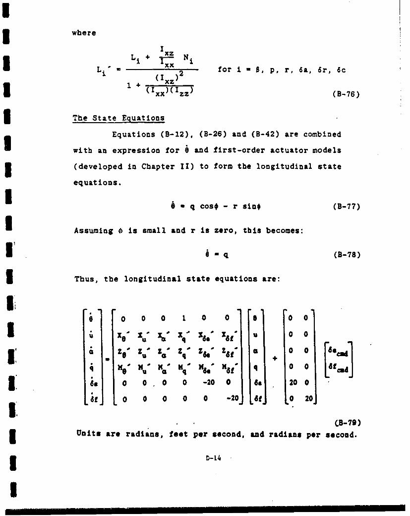
whereIxz

Li L Ixx for I B, p, r, 6a, 6r, 6c1 (Ixz) 2

0 Ixx zz (B-76)

The State Equations

Equations (B-12), (B-26) and (B-42) are combined

with an expression for 0 and first-order actuator models

(developed in Chapter II) to form the longitudinal state

equations.

6 a q cos# - r sinO (B-77)

Assuming 6 is small and r is zero, this becomes:

U = q (B-78)

Thus, the longitudinal state equations are:

I''9 0 0 0 1 0 0 a 0 0

zo o Z $ , ZO O Zq .Z S l Z f" a + 0 0 S

Me" Nu° Ma' Eq" 1 N 'e" XSf" q 0 0 £feaJ

3. o o 0 0 -20o0 . 200

61. 0 0 0 0 0 -20.o U6 %0 20

(B3-79)3 Units are radians, feet per second, and radians per second.

i D-L14

U

Equations (B-55), (5-73) and (B-73) are combined with

an 'xpression for ; and first-order actuator models to form

the lateral-directional state equations.

m * p + q sinO tane + r cos4 tans (B-80)

I Assuming e - 0 , this becomes:

S-inp (B-81)

Thus, the lateral-directional state equations are:

0 a 1 0 a0 00 00, vs," T, 1P I" Ta' T&I Tie, 0 0 0

0 LS- L, L€ 1,6f Lie' 0 00 6cad

0 P r 18 ia at r + 0 0 0 6rcmI

I. 0 0 0 0 -20 0 0 &a 20 00 4IcCad

a1 0 0 0 0 0 -20 0 It a 20 0

L i L 0 0 0 0 0 0 -20 1L 0 0 20

(B-S82)

1 These state equations must still be transformed as

shown in Chapter II to obtain longitudinal and lateral

accelerations an states. The stability azes coefficients

1must be converted to body axes coefficients for use in the

equations previously developed., The conversion equations

are *'

C! z (-C L .C D) Cooe2 T + -D82 in 2 UT

- + (-CL-CLCD a) cos" iT (B-83)

3 D-15Iv;

C Z CLC°S2.CoaT (B-83a)c a -TCosa (B-84)

q q3 Zu a (-CLu- 2 CL) Cos2aT + (CDe-CL) sin 2aT

+ ÷ (CL -CD u-CD) CosaT SndT (B-85)

z -iLaC osaT CCD6 sineT (B'86)3 C6 6

CX -c (-CDa+CL) Cos 2 aT + (CL u+2 CL) Sin2 a T

+ C-CD u-CD+CLa ) CosaT SinT (B.-87)

CXq - CLq SinaT (B-88)

3 CXu = (-CD u-2CD) Cos2T + (-CLO-CD) s1 2aOT

3 + (CD +CL CL) CoScT a (B-89)

C x =-CDa COSaT + CLa sinaT (B-90)

(CM mb - C1 a c00 + (CM +2 C) SifUC (B-91)

i(C.)b = c-m COGciy (B-92)

3 (C )b m (CM u+2CM) cosaT - Clia ,, (B-93)

D-16

U

(CMq)b - CMq (B-94)

(CM )b a CM6 (8-95)

where ( )b is used to distinguish body axes from stability

axes when necessary.

The equations for converting the lateral der~vatives

I to body axes are:

(CI )b =C Cosa T - Cn Sin T (B-96)

(t2 2

p (C )b - CL Cos T + sin aT

- (CL r+C V) snaT cos(-)

(CIr )b aCL r Cos 2 aT _ (Cs rp ) SinadT Cosa TC~~b" ~r- ta'tP) •Cap $in2aOT (B-98)

Ii pI (CL )b a Ct a - C(-99)

(Ca•)b a°Ca T +indT (B-100)

2(C a)b = C op S - (C n-Cp)Sina, Cosa,p p r p

- Cr sin2 aT (B-101)

I D- 17

I

(C r b= C n os 2aT +(C Ir +Cnp) sin* T Cosa T

+ Cr TP s)n2aT (B-102)

(Ca6 )b = Ca cosaT + C, a SinaT (B-103)

(C y )b= C (B-104)

(C ) cosaT y o C SITnaT .(B-105)

(Cyr )b Cyr CoSaT + Cyp SinaT (B-106)

I (C76)b = Cyd (B-107)

All of the computations to develop the body axes

3: primed derivatives from stability axes coefficients are per-

formed by the CAT program (see Appendix D).U1iscellaneous Equat ions

3 To convert inertias from the body axes to the sta-

bility axes, the following equations are used.

( xx)S (IX)B Cos 2 O+ ( 1Z)sB sin 2 2

-2(1 xz)B €osQT 01CT (B-108)

(I (zz)s- (jxx=) si~nS aT ('zz)B Can OT

+ 2(Ixz)B COSOT SinlOT (s-109)

5 D- 18

U

Ur xz)S . [(Ixx)B - (Izz)B] CosaT sinsT

+ (I xz)B (cOS 2 OT- sin2 OT (B-110)

where ( )S is used to denote the stability axes.

Accelerations at points other than the center of

5 gravity are calculated using:

txt

I (4. S( + qj) (B-ill)I~ ~ 2' 2

Ay~~ ~ r (T--)•÷ -Y (i ( r--)

I = yc

A+ -- -(B-112-)•

SAncg

++ (B-113)

Accelerations are in units of g, angular rates are in unitsI of degrees per second, and angular accelerations are in

5' degrees per second2 . The distances ix,. ty Lz are measured

in feet. The 1 x distance Is positiv, moving forward from

3 the CO along the x-axis. The Ly distance is positive along

the y-axis moving oet the right wing from the center of

I gravity. The Lz distance is positive along the z-axis or

3 down from the Cg.

3 D-(19

I aug urn

Angle of attack and angle of sideslip are expressed

as:

Stan(- ) and B " sin-( 1v (B-114)

where VT - (U 2 + V2 + W2 )* (B-1S)

D-20

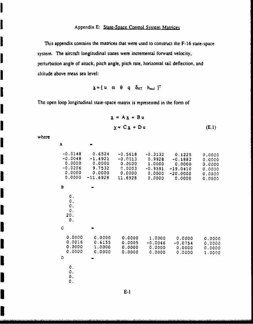
Appendix E: State-Space Control System Matrices

IThis appendix contains the matrices that were used to construct the F-16 state-space

system. The aircraft longitudinal states were incremental forward velocity,

perturbation angle of attack, pitch angle, pitch rate, horizontal tail deflection, and

j altitude above mean sea level:

& =[u CL 0 q 8 HT hm,, ]T

The open loop longitudinal state-space matrix is represented in the form ofI= AI + Bu

I Y= Cx + Du (E.1)

where-A 0

-0.0148 0.6524 -0.5618 -0.3132 0.1225 0.0000-0.0048 -1.4921 -0.0013 0.9928 -0.1882 0.00000.0000 0.0000 0.00o0 1.0000 0.0000 0.0000

-0.0206 9.7532 0.0003 -0.9591 -19.0410 0.00000.0000 0.0000 0.0000 0.0000 -20.0000 0.00000.0000 -11.6928 11.6928 0.0000 0.0000 0.0000

B 0

I o00.

20.00.I ~C

0.0000 0.0000 0.0000 1.0000 0.0000 0.00000.0016 0.6155 0.0005 -0.0046 -0.0754 0.00000.0000 1.0000 0.0000 0.0000 0.0000 0.00000.0000 0.0000 0.0000 0.0000 0.0000 1.0000

0.0.I 0.0.

E-1

I ___ _

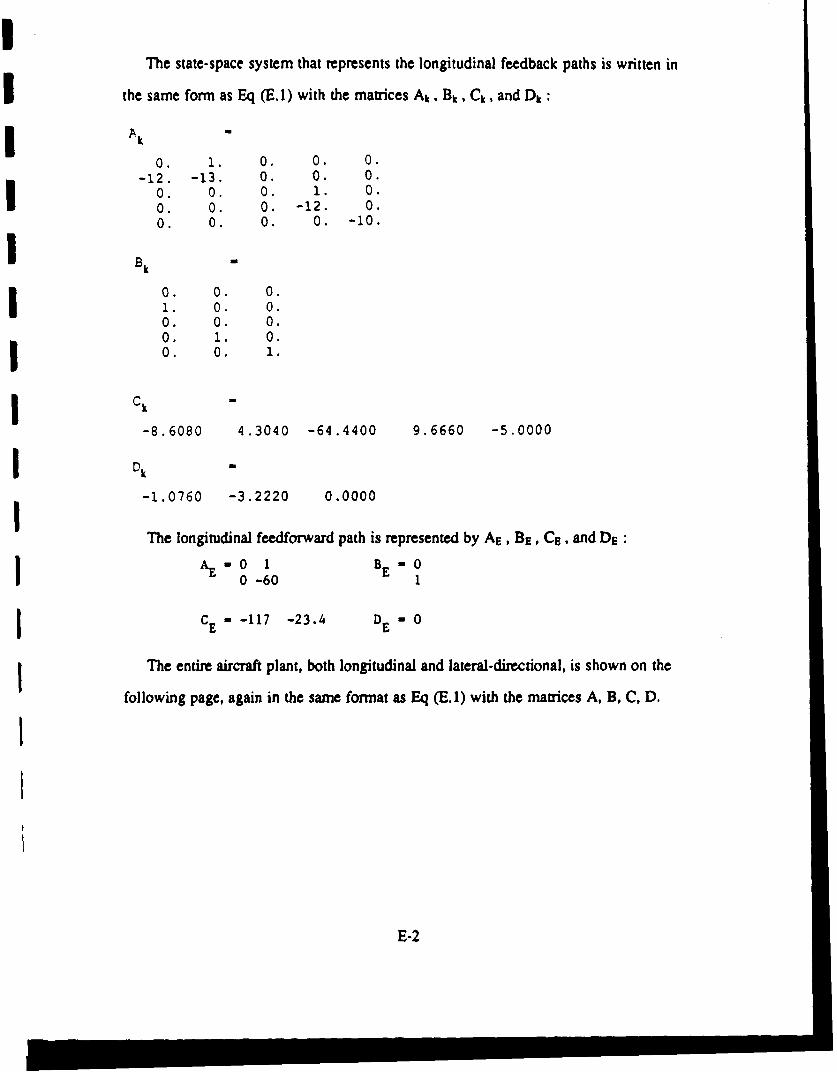
The state-space system that represents the longitudinal feedback paths is written in

the same form as Eq (E.1) with the matrices Ak. Bk, Ck, and Dk:

0. 1. 0. 0. 0.-12. -13. 0. 0. 0.

0. 0. 0. 1. 0.0. 0. 0. -12. 0.0. 0. 0. 0. -10.

Bk M

0. 0. 0.1. 0. 0.0. 0. 0.0. 1. 0.0. 0. 1.

Ck M

-8.6080 4.3040 -64.4400 9.6660 -5.0000

Dk

-1.0760 -3.2220 0.0000

The longitudinal feedforward path is represented by AE, BE, CE, and DE:

AE.0 1 BE -00 -60 1

CE - -117 -23.4 DE - 0

I The entire aircraft plant, both longitudinal and lateral-directional, is shown on the

following page, again in the same format as Eq (E.1) with the matrices A, B, C, D.

E-2

A -

Col..;7ns 1t'r-0.0148 0.0 c0 0.6524 0.0000 -0,5618 0. C OO: -0.O.O00 -0 .4391 0.000C 0.^300 0.00C0 0 .0490 0,023 2 ....004 0.0000 -1.4921 0.0000 -0.0013 0.00 0 0.00% c6

0.C0,: 0 .000 0.0000 0.0000 .00 0 OcO 0 . 1.00 • 0 , 0 O 0 0.00030 .O O 0.0000 0.0000 0 .000.0 1 001^1 0 .01^cO.OOCO -45.0950 0.0000 0.0000 0.0000 0.0000 -2 .469) 00* ^1-0.0206 0.000C 9.7532 0.0000 0.0003 0..000 0 .00^ -0.95;i0 .0000 7 .4884 0.0000 0.0000 0.0000 0.00:ý -0 30: 0.00c00 .0C00 0 .0000 0.0000 0.0000 0.0000 0.0000 0 0.•0 0.0;.':0.00 0 .0 0 0.000 0 .0 0000 0.0000 0.OOZ0 0."0;; 0.Occ:0 .0S0 0.00 0 0.0CCO0 :.000 0.0000 0.C00 0 .0.0000 0.0000 -11.6928 0.0000 11.6928 0.0:0 0o. Q 0.000.0.0560 0.000 11.4469 0.0000 0.0152 0.0000 0.0 00 0.0844

Columns 9 thr; 140.0000 0.1225 0.0000 P.0^00 0.0000 0.0000

-0.9956 0.0000 0.0047 0.0612 0.0000 0.00C00.0000 -0.1882 0.0000 0.0000 0.0000 0.00001.0000 0.0000 0.0000 0.0000 0.0000 0.00000.0000 0.0000 0.0000 0.0000 0.0000 0.00000.0000 0.0000 0.0000 0.0000 0.0000 0.0000

-0.0066 0.0000 -64.5965 11.3885 0.0000 0.00000.0000 -19.0410 0.0000 0.0000 0.0000 0.0000-0.8294 0.0000 -2.2082 -5.9140 0.0000 0.00000.0000 -20.0000 0.0000 0.0000 0.0000 0.00000.0000 0.0000 -20.0000 0.0000 0.0000 0.00000.0000 0.0000 0.0000 -20.0000 0.0000 0.00000.0000 0.0000 0.0000 0.0000 0.0000 0.00000.0000 2.2002 0.0000 0.0000 0.0000 0.0000

B

0. 0. 0.0. 0. 0.0. 0. 0.0. 0. 0.0. 0. 0.0. 0. 0.0. 0. 0.0. 0 .0.0 . 0. 0.

20. 0. 0.0 . 20. 0.0. 0. 20.0 . 0. 0.0. 0. 0.

Columns I thou 80.0000 0.0000 0.0000 0.0000 0.0000 0.0000 0.0000 1.00000.0016 0.0000 0.615S 0.0000 0.0005 0.0000 0.0000 -0.00460.0000 0.0000 0.0000 0.0000 0.0000 0.00000.0000 0.0000 0.0000 0.0000 0.0000 0.0000 1.0000 0.00000.0000 0.0000 0.0000 0.0000 0.0000 0.0000 0.0000 0.00000.0000 -0.1028 0.0000 0.0000 0.0000 0.0000 0.0000 0.0000

Columns 9 thru 140.0000 0.0000 0.0000 0.0000 0.0000 0.00000.0000 -0.0754 0.0000 0.0000 0.0000 0.00000.0000 0.0000 0.0000 0.0000 0.0000 0.00000.0000 0.0000 0.0000 0.0000 0.0000 0.00001.0000 0.0000 0.0000 0.0000 0.0000 0.0000

-0.0047 0.0000 -0.0149 -0.0224 O.Oofo n. lon0

D-0

* E-3

The states in the aircraft plant are incremental forward velocity, sideslip angle,

perturbation angle of attack, heading angle, pitch angle, bank angle, roll rate, pitch rate,

yaw rate, horizontal tail deflection, flaperua deflection, rudder deflection, altitude, and

altitude rate:

& [u =3 u Wt' 0 0 p q r 8HT 8 F 8R hmsi hmilIT

The complete feedback state-space system is represented by the matrices Ak, B1,

Ck, and Dk. The states in this case ae 'fictitious'.

AK

0. 1 0. 0. 0. 0. 0. 0. 0. . 0. 0.-12. -13. 0. 0. 0. 0. 0. 0. 0. 0. 0. 0.0. 0. 0. 1. 0. 0. 0. 0 0. 0. 0. 0.0. 0. 0. -12. 0. 0. 0. 0 0. 0. 0. 0.0. 0. 0. 0. -10. 0. 0. 0. 0. 0. 0. 0.0. 0. 0. 0. 0. -50. 0. 0. 0. 0. 0. 0.0. 0. 0. 0. 0. 0. 0. 1. 0. 0. 0. 0.0. 0. 0. 0. 0. 0. 0. 0. 1. 0. 0. 0.0. 0. 0. 0. 0. 0. -750. -815. -66. 0. 0. 0.0. 0. 0. 0. 0. 0. 0. 0. 0. 0. 1. 0.0. 0. 0. 0. 0. 0. 0. 0. 0. 0. 0. 1.0. 0. 0. 0. 0. 0. 0. 0. 0. -750. -815. -66.

BK

0. 0. 0. 0. 0. 0.1. 0. 0. 0. 0. 0.0. 0. 0. 0. 0. 0.0. 1. 0. 0. 0. 0.0. 0. 1. 0. 0. 0.0. 0. 0. 1. 0. 0.0. 0. 0. 0. 0. 0.0. 0. 0. 0. 0. 0.0. 0. 0. 1. 0. 0.0. 0. 0. 0. 0. 0.0. 0. 0. 0. 0. 0.0. 0. 0. 0. 1. 0.

CK -

Columns 1 thru 8-8.6080 4.3040 -64.4400 9.6660 -5.0000 0.0000 0.0000 0.00000.0000 0.0000 0.0000 0.0000 0.0000 -6.0000 0.0000 0.00000.0000 0.0000 0.0000 0.0000 0.0000 0.0000 -3.3174 11.6489

Columns 9 thru 120.0000 0.0000 0.0000 0.00000.0000 0.0000 0.0000 0.00002.8163 0.0000 -562.5000 -112.5000

DK 0

-1.0760 -3.2220 0.0000 0.0000 0.0000 0.00000.0000 0.0000 0.0000 0.0000 0.0000 0.00000.0000 0.0000 0.0000 0.0000 0.0000 -9.6600

E-4

The feedforward system for the complete system can be represented by the matrices

A., BE, Cr, and DE with DE being identically equal to zero:

AE

0. 1. 0. 0.0. -60. 0. 0.0. 0. -50. 0.C. 0. 0. -50.

BE

0. 0.1. 0.0. 1.0. 1.

CE

-11'7.000o -23.4000 0.0000 0.00000.0000 0.0000 -6.0000 0.00000.0030 0.0000 0.0000 -0.2216

I The closed loop state-space system for the aircraft can now be created using the

three state-space sytsems described above and the derivation presented in Chapter II of

I this thesis. Because of the size of the closed loop system. the representative matrices

are presented on the proceeding pages. The closed loop system is in the form of Eq

(E.1) with the matrices being ACL, Bc', Cc, and DCL , with DCL being identically

I equal to zero.

II

I E-5

,I - - - 1. ... . .. • . . .[- •

* A .

I-OD.04

CZ, IP. I^ . r^ ,• ... .. . ... . , -: . . .O-cocc c: .o~ ~ -"-000 0 . 303 0-.O- -0.0000 0-0.00 - . 0 0-00 0.:2 >.20.0:00 0.co00 0.3000 -3.ooo50 0.0000 0~.~ -30 ... •00. 30. O 0.6900 0.3000 0.0000 0.0030 0.0. *. : 00.0300 0.;000 0.0300 0.0300 0.3000 O.coco .00 0.0.0000 0.0300 0.C000 0.0000 0.0000) 0. 003 - 0 0.C0.o000 0.000.0 0. 0000 0.00c 000CC C.000 . 0 -c.0. 3000 0. 0000 0 . o00 3 .0000 0 .0000 0 .0.0.0.3000 0.0000 0.00,03 C.00c 0,000c 0 C. -.0.:000. 0 -. 0 c: : 3 . 0 .0 0 0 .. 3000.0: .2 : C : :

0.0000 000 C :3 0 .-0.-2340 -0.0468 0.0:00 0.C000 0.000c 0.000.O.O0oc 0.0':00 -0.012o co0 0 00o 0 ^• ,3o

0 .0000 ,C. 303 0,.32 , -2 . 3000 0_ 000 -0. >020 3..030^ 0. ;0.0000 0.0300 0.0300 3300 >0000 0.3000 -32 12 0.33000.0000 0.0000 0.00 00 0.0000 0.0000 0.0000 ..•.1.0.:0,0000 0.0000 0.0000 0.0000 0.0000 0.0000 0.000 0.00000.0000 0.0000 0.0000 0.0000 0.0000 0.0000 0.0000 0.00000.0000 0.0000 0.0000 0.0000 0.0000 0.0000 0.0000 0.00000.0000 0.0000 0.0000 0.0000 0.0000 0.0000 0.0001 0.00000.0000 0.0000 0.0000 0.0000 0.0000 0.0000 0.0000 0.00000.0000 0.0000 0.0000 0.0000 0.0000 0.0000 0.0000 0.00000.0000 0.0000 0.0000 0.0000 0.0000 0.0000 0.0000 0.00000-0000 0.0000 0.0000 0.0000 0.0000 0.0000 0.0000 0.00000.0000 0.0000 0.0000 0.0000 0.0000 0.0000 0.0000 0.00000.0000 0.0000 0.0000 0.0000 0.0000 0.0000 0.0000 0.00000.0000 0.0000 0.0000 0.0000 0.0000 0.0000 0.0000 0.00000.0000 0.0000 0.0000 0.0000 0.0000 0.0000 0.0000 0.0000Columns 9 thru 16

0.0000 0.0000 0.0000 0.0000 0.0000 0.0000 0.0000 0.00000.l000 0.0000 0.0000 16 0.000 0 0.000 0.000.0000 0.0000 0.0000 0.0000 0.0000 0.0000 0.0000 0.0000-0.000 0.0000 0.0000 0.0000 0.0000 0.0000 0.0000 0.0000-0.0000 0.0000 0.0000 0.0000 0.0000 0.0000 0.0000 0.00000.0000 0.0000 0.0000 0.0000 0.0000 0.0000 0.0000 0.00c00.0000 0.0000 0.0000 0.0000 0.0000 0.0000 0.0000 0.00000.0000 0.0000 0.0000 0.0000 0.00001 0.0000 0.0000 0.00000.0000 0.0000 0.0000 0.0000 0.0000 0.0000 0.0000 0.00000.0000 0.0000 0.0000 0.0000 0.0000 0.0000 0.0000 0.00000.0000 0.0000 0.0000 0.0001 0.0000 0.0000 0.0000 0.00000.0000 0.0000 0.0000 0.0000 0.0000 0.0000 0.0000 0.00000-0000 0.0000 -0.0002 0.0000 -0.0000 0.0000 -0.0002 -. 000.0000 0.0000 0.0000 0.0021 0.0000 -0.0025 0.0000 000000.0000 0.0000 0.0000 0.0000 0.0000 0.0000 -0.0020 0.00000.0000 0.0000 0.0000 0.0000 -0.0001 0.0000 -0.0003 -0.00240 . 0 2 0 0 0 . 000.000 0 0 .0 0 0 0 0 .0 0 0 0 -0 .00 0 02 -0 .000 06000 0.00 0.0000 0.0021 0.0000 -0.0002 0.0000 0.0000

0.0000 0.0000 0.0000 0.0000 0.0000 0.0000 0.0000 0.00000.0000 0.0000 0.0000 0.0000 0.0001 0.0000 -0.0003 -00020.0000 0.0000 0.0000 0.0000 0.0000 0.0000 0.0000 0.00000.0000 0.0000 0.0000 0.0000 0.0000 0.0000 0.0000 0.00000.0000 0.0000 0.0000 0.0000 0.0000 0.0000 0.0000 0.00000.0000 0.0000 0.0000 0.0001 0.0000 0.0000 0.0000 0.00000.0000 0.0000 0.0000 0.0000 0.0000 0.0000 0.0000 0.00000.0000 0.0000 0.0000 0.0000 0.0000 0.0000 0.0000 0.00000.0000 0.0000 0.0000 0.0000 0.0000 0.0000 0.0000 0.00000.0000 0.0000 0.0000 0.0000 0.0000 0.0000 0.0000 0.00000.0000 0.0000 0.0000 0.0000 0.0000 0.0000 0.0000 0.0000

0.0000 0.0000 0.0000 0.0000 0.0001 0.0000 0.0000 0.0000

I-

o.'*::o 0.o•o: 0.0•o: C.::oo 0.0000 0.003 3.O000: 0.0:::c . .. - ... 3.000: .9 . O cO , :.. •:0 0% 3 0.2:: J. 0 0.0000 c. , ^00 .

0.::o ,o.oo3o 0.32:: :.::oo 0.03000 0.;33: . oc0•0 .O:C 0.0000 0 0 .0 0 0 .0.Z'0 -. 030C

0000 0.2:: 0.0000 0.0000 0.000 ; .00 c0.03C 0 0.0000 O.CZOo 0.0000 0.0000 0,0000 0.0000 0.0C.0 0 0000 0.0; 0 -0.000I 0.000. .0.0000 0C0 00 00c00.0...o 0.0000 0.0C00 0.0000 0.0000 0.0000 0.0000 0,000.0- 0 C 0.00 0 00 0.0000 0.0000 0.0000 c.0000 0.000,0.00c0 0.0000 0.C3OC 0.0000 0.0000 0.0000 0,000 .0030.0000 0.0000 0.0020 0.0000 0.0000 000 0 .00C.0 . 03 ). CO 90 0 . 0 0 0 . 00 0 .0 20.00 0.0000 0 .0000 0.0000 0.0000 0.0000 0.0000 0.0000.OO1O 0.0000 0..000 - -0.0 0000.0300 0.0000 0.0000 0.OC::0.0000 0.0000 0.0003 0.6000 0.0000 0.000: 0.0000 0.-0 •0.0000 0.0000 0.0: o.C 0.0001 -0.012 0.00CO 0.000 00.0g10 0. 0.032 .C1 00 0 0.0000 -0.C0500.0000 00oc . 000 0 .0000 CO000 0.0000 0.03 0 -00000 0.C0CO^0 0 0 w0 0.ý -) - 0000 0,0000 0.000 0.0000 0.00000.0000 0.0000 0.0000 0.0000 0.0000 0.0000 0.0000 0.00000.000 0000 0.0000 0.00 0,0000 0.000 0.0000 0.00000.0000 0.0000 0.0000 0.0000 0.0000 0.0000 0.0000 0.00000.0000 0.0000 0.0000 0.0000 0,0000 0.0000 0.0000 0.00000.0000 0.0000 0.0000 0.0000 0.0000 0.0000 0.0000 0.00003 ~ ~~~~Columns 25 thru 30 000 .00 0000.0000 0.0000 0.0000 0.0000 0.0000 0.00000.0000 0.0000 0.0000 0.0000 0.0000 0.00000.Colu 0.0000 0.0000 0.0000 03000 0.00000.0000 0.0000 0.0000 0.0000 0.0000 0.00000.0000 0.0000 0.0000 0.0000 0.0000 0.00000.0000 0.0000 0.0000 0.0000 0.0000 0.00000.0000 0.0000 0.0000 0.0000 0.0000 0.00000.0000 0.0000 0.0000 0.0000 0.0000 0.00000.0000 0.0000 0.0000 0.0000 0.0000 0.00000.0000 0.0000 0.0000 0.0000 0.0000 0.0000

0.0000 0.0000 0.0000 0.0000 0.0000 0.00000.0000 0.0000 0.0000 0.0000 0.0000 0.00000.0000 0.0000 0.0000 0.0000 0.0000 0.00000.0000 0.0000 0.0000 0.0000 0.0000 0.00000.0000 0.0000 0.0000 0.0000 0.0000 0.00000.0000 0.0000 -0.0000 0.0000 0.0000 0.00003o.00ooo o'o0o, 0.0000 0.0000 0.0000 o0.ooo0.0000 0.00 0.0000 0.0000 0.0000 0.0000O.OOC 0.0000 0.0000 0.0000 0.0000 0.0000o.oo00 -0.0000 -0•000 0.0000 0.0000 0.20000.0000o 0.0000 0.0000 0.0000 0.oooo 0.00000.o0 0.00010 0.0000 0.0000 0.0000 0.00000.Ooooo 1,0 ý 0.0000 0.0000 0.0000 0,oo .00000.0000 o.o6ýo0 0.0000 0.0000 0.0000o 0.00000.O000 0.0000 0.0000 0.0000 0.0000 0.00000.0000 0.0000 0.0000 0.0000 0.0000 0.0000

-0.0750 -0.0800 -0.0066 0.0000 0.0000 0.00000.0000 0.0000 0.0000 0.0000 0.0000 0.0001

0.0000 0.0000 0.0000 -0.0750 -0.0815 -0.0066

0. 0.0. 0.0. 0.0. 0.0. 0.0. 0.0. 0.0. 0.0. 0.0. 0.0. 0.0. 0.0. 0.0. 0.0. 0.0. 0.0. 0.

0. 0.0., 0.0. 0.0. 0.0. 0.0. 0.0. 0.0. 0.0. 0.

0 0.0.000 0.00 0 0.00 0 00 0 . 0 0 00 0 .~ o 000.0 00 0. Q' ~ C.~0 0. 0 0 0. 0 6 . 0 o 0. 1 5 . 00

o~~or~~c. ~O O.O O 0. 0 0 00 0 0. 0 0 .0 0 1. 00 . 0 00.0000 0.0 00 .0 0 0. 0 0 0. 0 0 . 00 000 0 .0 oColumns I thru 80.0000 0.0000 0.0000 0.0000 0.0000 0.0000 0.0000 0.0oc0

0.0000 0.00-I 0.0000 0.0000 0.0016 0.0000 0.6155 0.00000.0O C 0 O.C0 0.0000 0.0000 0.0000 0.0000 0.0000 0.00000.0000 0.0000 0.0000 0.0000 0.0000 0.0000 0.0000 0.00000.0000 0.0000 0.0000 0.0000 0.0000 0.0000

0 00 0 00o0.0000 0.0000 -0.0040 0.0000 -0.004 00 22

0.00 .noAA A nAAA A MAMA A AMAIN 0*0000^•^ •

Columns 9 thru 16 2A^'0.0000 0.0000 0.0000 1.0000 0.0000 0.0000 0.0000 0.00000.00.00 00.0000 * 00.000 00 000 00.000 0.0000 0.00000.0000 0.0000 0.0000 0.0000 0.0000 0.0000 0.0000 0.00000.0000 0. 00 .0000 0.0000 0.0000 0.0000 0.0000 0.00000.0000 0 .00 0.0000 0.0000 0.0000 0.00 0. 0 0 .00000.0000 0.0000 0.00000 0. 0.00 00 .0000 0.0000 0.0000

0.0000 0.0000 0.0000 0.0000 0.0000 0.0000 0.00000.0000 0.0000 0.0000 0.0000 0.0000 0.0000

0.0000 0.0000 0.0000 0.0000 0.0000 0.0000 0.0000 0.00000.0000 0.00000 0.0000 0.0000 0.00000.0000 0.0000 0.0000 0.0000 0. 0.0000 0.0000 0.00000.000- 0.0000 000000 0.0000 0.0000 0.0000 0.0000 0.00000000.00000 0.0000 0.0000 0.0000 0.0000 0.00000.00 00 00000 0.0000 0.0000 0.0000 0.0000 0.00000-000.0000 0.0000 0.0000 0 -0000 0.0000 0.00000.0000 0.0000 0.0000 0.0000 0.0000 0.00000.O0000 0.0000 0.0000 0.0000 0.000 0.0000

0.0000 0.00c0 0.0000 0.0000 0.0000 0.0000

I 0 00

The eigenvalues, or poles, of the open loop plant are

0.0000 + 0.0000i0.0000 + 0.0000i0.0000 + 0.O000i

-0.0086 + 0.0719i-0.0086 - 0.0719i-0.0822 - 0 .0000i1.9006 - 0.O000i

-2.4504 + 0.O000i-0.6024 + 2.9269i-0.6024 - 2.9269i-4.3494 + 0.O000i

-20.0000 + 0.O000i-20.0000 + 0.0000i-20.0000 + 0.O000i

The eigenvalues of the closed loop system are given by

0.0000 + 0.O000i0.0000 + 0.0000i0.0000 + 0.O0000i0.0000 + 0.0000i

-0.0002 + 0.O000i-0.0123 + 0.O000i-0.0149 + 0.0000i-0.6415 + 0.0000i-1.0000 + 0.0000i-1.3308 + 0.0000i-2.1112 + 0.0000i-1.4835 - 2.21871-1.4835 + 2.21871-3.3356 + 3.1843i-3.3356 - 3.1843i

-10.2819 + 0.0000i-12.0000 -.0.00001

-9.0094 -10.46681-9.0094 +10.46681

-15.0000 + 0.0000i-14.3102 -16.43491

-14.3102 +16.43491-15.3023 -15.64131-15.3023 +15.6413i-50.0000 - 0.0000i-50.0000 + 0.0000i-50.0000 + 0.0000±-54.4802 - 0.0000i

-58.6432 - 0.0000i-60.0000 + 0.O000i

E-9

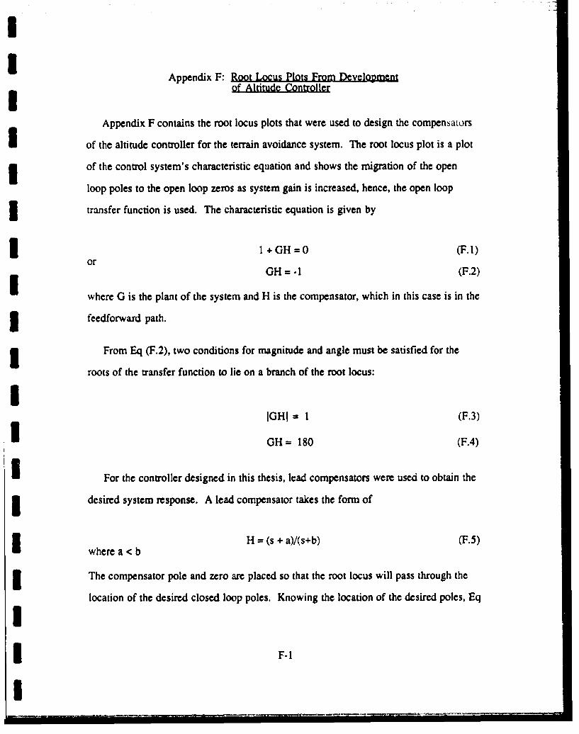
Appendix F: Root Locus Plots From Developmentof Altitude Controller

Appendix F contains the root locus plots that were used to design the compensaLors

of the altitude controller for the terrain avoidance system. The root locus plot is a plot

of the control system's characteristic equation and shows the migration of the open

loop poles to the open loop zeros as system gain is increased, hence, the open loop

3 transfer function is used. The characteristic equation is given by

1+GH =0 (F.I)or

GH= -1. (F.2)

where G is the plant of the system and H is the compensator, which in this case is in the

3 feedforward path.

U From Eq (F.2), two conditions for magnitude and angle must be satisfied for the

roots of the transfer function to lie on a branch of the root locus:

UIGHI = I (F.3)

_ GH= 180 (F.4)

* For the controller designed in this thesis, lead compensators were used to obtain the

3 desired system response. A lead compensator takes the form of

w H = (s + a)/(s+b) (F.5)I where a < b

3 The compensator pole and zero are placed so that the root locus will pass through the

location of the desired closed loop poles. Knowing the location of the desired poles, Eq

F3 F-1

I

(F.4) can be used to design the compensator. For a lead compensator, the zero location

is usually chosen, and then Eq (F.4) is used to determine the location of the pole. A

lead compensator in the forward path will tend to pull the branches of a root locus fur-

ther over into the left-half plane, while a lag compensator will have the opposite effect.

Once the locus passes through the desired poles, the compensator gain is adjusted until

the desired poles are reached. The location of these poles will become the poles of the

closed loop system.

The design method discussed above was used in the design of the altitude controller

for this thesis. A more detailed discussion of the compensators chosen for this design

is given in Chapter III.

S~F-2

I

I0

Ir 0

1 ~04.

U 0~

1 04

F-3I

0I

F-44

I1

m op

F-5-

00

S A

- 0o

III

--5

l -- ' .. . ... ...... .. i . ... i .. . . . . . r " i I I I

I X-O

0

*u 0

SCL0 IJ 0

0

00

*s

Co opCo U10 So

W-4 --

%xv. s 4= -0-

F-6

I~ ow

co w

80

0

0

00

*W*

I F-7

0 ai*j cc

*0-4

F-84

ii

0

0

0

F-9-

0

I

0

0

3 0

am

F-10

F-IOb

bjj q

I Bibliography

I 1. Skoog, Mark A. and ILt. Gregory W. Bice. AFrIIF-16 AMAS Ground CollisionAvoidance System Evaluation. AFFTC-TR-87-11. Edwards AFB, CA: Air ForceI Flight Test Center, August 1987.

2. Roskam, Jan. Airplane Flight Dynamics and Automatic Flight Controls. Part 1.Ottawa, Kansas: Roskarn Aviation and Engineering Corporation, 1979.

3. McRuer, Duane et al. Aircraft Dynamics and Automatic Control. Princeton, NewJersey: Princeton University Press, 1973.

4. USAF Test Pilot School. Flying Oualities Textbook.Vol. II.Part 2. USAFTPS-CDR-86-03. Edwards AFB, CA: USAFTPS, April 1986 (AD-A170960).

5. Reid, J. Gary. Linear Systems Fundamentals. New York: Mcgraw- Hill, Inc.,1983.

6. Thompson, Peter M. Program CC Manual, Version 3.0. Systems Technology Inc.,Hawthorne, California, 1985.

7. MATRIXx Program Manual, Version 7.0. Integrated Systems Ihc., Santa Clara,California, October 1988.

8. Barfield, A. Finley. Multivariable Control Laws for the AFIIF-16. MS thesis,AFIT/GE/EE/83S-4. School of Engineering, Air Force Institute of Technology(AU), Wright-Patterson AFB OH. July 1983.

IIIIIII

I Bib-1

I

Captain Gregory W. Bice was born on 2 September 1962 in Hays, Kansas. He

I graduated from high school in Beloit, Kansas, in 1981 and entered the United States

Air Force Academy, receiving a Bachelor of Science degree in Aeronautical Engineer-

ing in May 1985. Upon graduation, he reported to the Air Force Flight Test Center at

I Edwards AFB, California, where he served as a flight dynamics engineer with the

6520th Test Group. Captain Bice was assigned to the Advanced Fighter Technology

Integration (AFTI) / F- 16 Joint Test Force where he worked on the development and

flight testing of automated attack and ground collision avoidace systems, receiving a

patent for his design of an automated ground collision avoidance system. He entered

I the School of Engineering, Air Force Institute of Techology, in June 1988.

Permanent address: 718 Colonial Ct.

Salina, Kansas 67401

IIIII!III V-i

I

UNCLASSIFIEDSECURITY-CLASSIFICATION OF THIS PAGE

Form AWprvecREPORT DOCUMENTATION PAGE OMONo.A0704-0

11 REPORT SECURITY CLASSIFICATION lb RESTRICTIVE MARKINGS

UNCLASSIFIED24. SECURITY CLASSIFICATION AUTHORITY 3. DISTRIBUTION/AVAILABILITY OF REPORT

2b. DECLASSIFICATION/DOWNGRADING SCHEDULE Approved for public release;

distribution unlimited4. PERFORMING ORGAN. 'c ION REPORT NUMBER(S) S. MONITORING ORGANIZATION REPORT NUMBER(S)

AFIT/GAE/ENY/89D-03

". NAME OF PERFORMING ORGANIZATION 6b. OFFICE SYMBOL 7.. NAME OF MONITORING ORGANIZATION(If applicable)

School of Engineering AFIT/ENG

6c. ADDRESS (City, State, and ZIPCode) 7b. ADDRESS (City, State, and ZIP Code)

Air Force Institute of Technology

Wright-Patterson AFB OH 45433-6583I S. NAME OF FUNDING/SPONSORING 8b. OFFICE SYMBOL 9. PROCUREMENT INSTRUMENT IDENTIFICATION NUMBERORGANIZATION (If applicable)

Controls Applications Group WRDC/FIGX

&. ADDRESS (City, State, and ZIP Code) 10. SOURCE OF FUNDING NUMBERS

PROGRAM PROJECT TASK WORK UNITFlight Dynamics Laboratory ELEMENT NO. NO. NO CCESSION NO.

Wright-Patterson AFB OH 45433-6583 r1 . TITLE (Include Security Classification)

DEVELOPMENT OF AN AUTOMATIC GROUND COLLISION AVOIDANCE SYSTEM

USING A DIGITAL TERRAIN DATABASE12. PERSONAL AUTHOR(S)

Gregory W. Bices B.S., Capt, USAF13a. TYPE OF REPORT 13b. TIME COVERED 14. DATE OF REPORT (Year, Month, Day) 115. PAGE COUNT

MS Thesis FROM TO 1989 December 151116. SUPPLEMENTARY NOTATION

17. COSATI CODES 18. SUBJECT TERMS (Continue on revere If necessary and identify by block number)FIELD GROUP SUB-GROUP F-16 Aircraft Autopilot Terrain Avoidance

01 02 O0 Automatic Ground Collision Avoidance Systems (GCAS)01 03 12 Controlled Flight Into Terrain (CFIT)

19. ABSTRACT (Continue on revere if necessary and Identify by bloKk number)

Thesis Advisor: Capt Curtis P. Mracek

Associate Professor

Department of Aeronautics and Astronautics

Ii

20. DISTRIBUTION/ AVAILABILITY OF ABSTRACT 21. ABSTRACT SECURITY CLASSIFICATIONtUNCLASSIFIED/UNLIMITED 03 SAME AS RPT. ] DTIC USERS UNCLASSIFIED

22a. NAME OF RESPONSIBLE INDIVIDUAL 22b. TELEPHONE (Include Area Code) 22c OFFICE SYMBOLI Curts P. Mracek Assoc. Professor (513) 255-3517 ENY

DO Form 1473, JUN 86 Previous editions are obsolete. SECURITY CLASSIFICATION OF THIS PAGE

UNCLASSIFIED

UNCLASSIFIED

During the past several years, the Air Force has experienced an

increasing number of single seat aircraft mishaps due to what is termed

'controlled flight into terrain'. To combat this phenomenon, several

ground collision avoidance systems (GCAS) have been developed to warn

the pilot of a potential collision with the terrain if some action

is not taken c-uw-eVAr,. all current systems have shortcomings pertaining

to the sensors that are used and the recovery maneuver that is flown.

The USAF is evaluating the potential of digital terrain databases for

onboard navigation and terrain avoidance in combat aircraft. The pur-

pose of this thesis was to develop a control system for performing

terrain avoidance using a simulated terrain database. This study was

conducted for an F-16 aircraft in level flight at 0.6 Mach and sea

level conditions. A state-space model of the aircraft and its flight

control system was developed using aircraft control derivatives, an

F-16 control law diagram, and traditional linearization techniques on

the aircraft equations of motion. A control system for implementing

terrain avoidance was derived based on the look-ahead capability of

the terrain database. Control system response was evaluated using a

simulated terrain obstacle and various look-ahead distances on the

terrain database. Results indicated that a 1200 foot, or roughly 1.8 m

second, look-ahead distance provided good improvement in terrain

avoidance capabilities for the F-16 compared to looking strictly

downward from the aircraft for terrain information.

IIIIIII

UNCLASSIFIEDm

"1 0

DTIC iw