Institute for Mathematical Sciences

National University of Singapore

BRAIDS: summer school and workshop

Tutorial: Braids - definitions and braid groups

June 4-8, 2007

Dale Rolfsen

Department of Mathematics

University of British Columbia

Vancouver, BC, Canada

rolfsen@math.ubc.ca

1

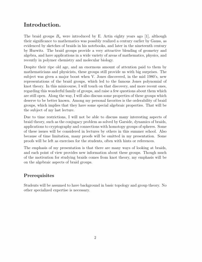
Introduction.

The braid groups Bn were introduced by E. Artin eighty years ago [1], althoughtheir significance to mathematics was possibly realized a century earlier by Gauss, asevidenced by sketches of braids in his notebooks, and later in the nineteenth centuryby Hurwitz. The braid groups provide a very attractive blending of geometry andalgebra, and have applications in a wide variety of areas of mathematics, physics, andrecently in polymer chemistry and molecular biology.

Despite their ripe old age, and an enormous amount of attention paid to them bymathematicians and physicists, these groups still provide us with big surprises. Thesubject was given a major boost when V. Jones discovered, in the mid 1980’s, newrepresentations of the braid groups, which led to the famous Jones polynomial ofknot theory. In this minicourse, I will touch on that discovery, and more recent ones,regarding this wonderful family of groups, and raise a few questions about them whichare still open. Along the way, I will also discuss some properties of these groups whichdeserve to be better known. Among my personal favorites is the orderability of braidgroups, which implies that they have some special algebraic properties. That will bethe subject of my last lecture.

Due to time restrictions, I will not be able to discuss many interesting aspects ofbraid theory, such as the conjugacy problem as solved by Garside, dynamics of braids,applications to cryptography and connections with homotopy groups of spheres. Someof these issues will be considered in lectures by others in this summer school. Alsobecause of time limitation, many proofs will be omitted in my presentation. Someproofs will be left as exercises for the students, often with hints or references.

The emphasis of my presentation is that there are many ways of looking at braids,and each point of view provides new information about these groups. Though muchof the motivation for studying braids comes from knot theory, my emphasis will beon the algebraic aspects of braid groups.

Prerequisites

Students will be assumed to have background in basic topology and group theory. Noother specialized expertise is necessary.

2

Suggested reading

• Joan Birman and Tara Brendle, Braids, A Survey, in Handbook of Knot Theory (ed.W. Menasco and M. Thistlethwaite), Elsevier, 2005.

Available electronically at:

http://www.math.columbia.edu/ jb/Handbook-21.pdf

• Joan Birman, Braids, links and mapping class groups, Annals of Mathematics Stud-ies, Princeton University Press, 1974.

This classic is still a useful reference.

• Gerhard Burde and Heiner Zieschang, Knots, De Gruyter Studies in Mathematics5, second edition, 2003.

This contains a very readable chapter on braid groups.

• Patrick Dehornoy, Ivan Dynnikov, Dale Rolfsen, and Bert Wiest, Why are braidsorderable? Soc. Math. France series Panoramas et Syntheses 14(2002).

Available electronically at:

http://perso.univ-rennes1.fr/bertold.wiest/bouquin.pdf

• Vaughan F. R. Jones, Subfactors and Knots, CBMS Regional Conference series inMathematics, Amer. Math. Soc., 1991.

This gem focusses on the connection between operator algebras and knot theory, viathe braid groups.

• Vassily Manturov, Knot Theory, Chapman & Hall, 2004.

The most up-to date text. Contains details, for example, of the faithfulness Bigelow-Krammer-Laurence representation.

• Kunio Murasugi and Bohdan Kurpita, A study of braids, Mathematics and itsapplications, Springer, 1999.

Also see research papers and other books in the bibliography at the end of the notes.

3

1 Braids as strings, dances or symbols:

One of the interesting things about the braid groups Bn is they can be defined inso many ways, each providing a unique insight. I will briefly describe some of thesedefinitions, punctuated by facts about Bn which are revealed from the various pointsof view. You can check the excellent references [1], [2], [5], [7], [10], [15] for moreinformation.

Definition 1: Braids as strings in 3-D. This is the usual and visually appealingpicture. An n-braid is a collection of n strings in (x, y, t)-space, which are disjointand monotone in (say) the t direction.

We require that the endpoints of the strings are at fixed points, say the points (k, 0, 0)and (k, 0, 1), k = 1, . . . , n. We also regard two braids to be equivalent (informally,we will say they are equal) if one can be deformed to the other through the family ofbraids, with endpoints fixed throughout the deformation.

Although most authors draw braids vertically, I prefer to view them horizontally withthe t-axis running from left to right. My reason is that we do algebra (as in writing)from left to right, and the multiplication of braids is accomplished by concatenation(which is made more explicit in the second definition below), which we take to be inthe same order as the product. In the vertical point of view, some authors view theproduct αβ of two braids α and β with α above β, while others would put β on topof α. The horizontal convention eliminates this ambiguity.

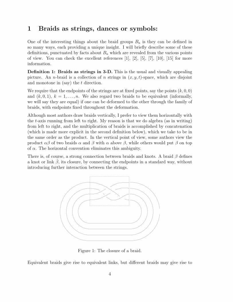
There is, of course, a strong connection between braids and knots. A braid β definesa knot or link β, its closure, by connecting the endpoints in a standard way, withoutintroducing further interaction between the strings.

Figure 1: The closure of a braid.

Equivalent braids give rise to equivalent links, but different braids may give rise to

4

the same knot or link. We will discuss how to deal with this ambiguity later. Bn willdenote the group formed by n-braids with concatenation as the product, which wewill soon verify has the properties of a group, namely an associative multiplication,with identity element and inverses.

Definition 2: Braids as particle dances. If we take t as a time variable, then abraid can be considered to be the time history of particles moving in the (x, y) plane,or if you prefer, the complex plane, with the usual notation x + y

√−1.

This gives the view of a braid as a dance of noncolliding particles in C, beginningand ending at the integer points {1, . . . , n}. We think of the particles moving intrajectories

β(t) = (β1(t), . . . βn(t)), βi(t) ∈ C,

where t runs from 0 to 1, and βj(t) 6= βk(t) when j 6= k. A braid is then such atime history, or dance, of noncolliding particles in the plane which end at the spotsthey began, but possibly permuted. Equivalence of braids roughly reflects the factthat choreography does not specify precise positions of the dancers, but rather theirrelative positions. However, notice that if particle j and j + 1 interchange places,rotating clockwise, and then do the same move, but counterclockwise, then theirdance is equivalent to just standing still!

The product of braids can be regarded as one dance following the other, both atdouble speed. Formally, if α and β are braids, we define their product αβ (in thenotation of this definition) to be the braid which is α(2t) for 0 ≤ t ≤ 1/2 and β(2t−1)for 1/2 ≤ t ≤ 1.

Exercise 1.1 Verify that the product is associative, up to equivalence. The identitybraid is to stand still, and each dance has an inverse; doing the dance in reverse. Moreformally, if β is a braid, as defined in this section, define β(t) = β(1 − t). Write aformula for the product γ = ββ and verify that there is a continuous deformationfrom γ to the identity braid. [Hint: let s be the deformation parameter, and considerthe dance which is to perform b up till time s/2, then stand still until time 1 − s/2,then do the dance β in the remaining time.]

A braid β defines a permutation i → βi(1) which is a well-defined element of thepermutation group Σn. This is a homomorphism Bn → Σn with kernel, by definition,the subgroup Pn < Bn of pure braids. Pn is sometimes called the colored braid group,as the particles can be regarded as having identities, or colors. Pn is of course normalin Bn, of index n!, and there is an exact sequence

1 → Pn → Bn → Σn → 1.

Exercise 1.2 Show that any braid is equivalent to a piecewise-linear braid. Moreover,one may assume that under the projection p : R3 → R2 given by p(x, y, t) = (y, t),

5

there are only a finite number of singularities of p restricted to the (image of the)given braid. One may assume these are all double points, where a pair of stringsintersect transversely, and at different t-values.

Figure 2: Equivalent braids.

Exercise 1.3 Viewing the projection in the (y, t) - plane, with the t-axis as hori-zontal, for any fixed value of t at which a crossing does not occur, label the strings1, 2, . . . , n counting from the bottom to the top in the y direction. Let σi for i =1, . . . , n − 1 denote the braid with all strings horizontal, except that the string i + 1crosses over the i string, resulting in the permutation i ↔ i + 1 in the labels of thestrings. (Think of it as a right-hand screw motion of these two strings. Argue that anybraid is equivalent to a product of these “generators” of the braid group. [In Figure1, for example, the braid could be written either as σ−1

2 σ−11 σ3σ2σ

−11 or σ−1

2 σ3σ−11 σ2σ

−11

(or indeed many other ways).]

Finally, note that the inverse of σi is the braid with all strings horizontal, except thatthe string i crosses over the i+1 string. The first sketch in Figure 2 shows that theseare indeed inverse to each other.

Definition 3: The algebraic braid group. Bn can be regarded algebraically asthe group presented with generators σ1, . . . , σn−1, where σi is the braid described inthe previous exercise. These generators are subject to the relations (as suggested inFigure 2:

σiσj = σjσi, |i− j| > 1,

σiσjσi = σjσiσj, |i− j| = 1.

It was proved by Artin that these are a complete set of relations to abstractly defineBn. This means that any relation among the σj can be deduced from the aboverelations.

6

Exercise 1.4 Verify that, in Bn, all the generators σj are conjugate to each other.Show the total degree deg(β) which is the sum of the exponents which appear in anexpression of β in the σj, is well-defined, i.e. independent of the expression. Verifythat the abelianization of Bn, for n ≥ 2, is the infinite cyclic group Z, and deg : Bn →Z is equivalent to the abelianization homomorphism. Thus the commutator subgroupof Bn consists of all words of total degree zero.

Exercise 1.5 In B3, consider the special element ∆ = ∆3 = σ1σ2σ1, which consistsof a clockwise “half-twist” of the three strings. Verify that ∆σ1 = σ2∆ and ∆σ2 =σ1∆. Conclude that ∆2 commutes with both generators of B3 and therefore is in thecentre of B3. (It actually generates the centre, but we will not prove this.)

Show that in B3 there are two braids α and β such that α 6= β but α3 = β3. Whatabout squares?

Exercise 1.6 For n ≥ 3, define γ = γn = (σ1σ2 · · ·σn−1)n. Draw this braid and

convince yourself that it is a “full-twist” and that γ is central in Bn.

In fact γn generates the (infinite cyclic) centre of Bn.

We can take a whole countable set of generators σ1, σ2, . . . subject to the aboverelations, which defines the infinite braid group B∞. If we consider the (non-normal)subgroup generated by σ1, . . . , σn−1, these algebraically define Bn. Notice that thisconvention gives “natural” inclusions Bn ⊂ Bn+1 and Pn ⊂ Pn+1.

Exercise 1.7 Does B∞ have a nontrivial centre?

Going the other way, if one forgets the last string of an n + 1-braid the result is ann-braid. But strictly speaking, this is only a well defined homomorphism for purebraids, (or at best for the subgroup of braids in which the string beginning at thepoint n + 1 also ends there). Later, we will have a use for this forgetful map

f : Pn+1 → Pn

It is easy to see that f is a left inverse of the inclusion, or in other words a retractionin the category of groups.

Artin Combing. We now have the ingredients for the combing technique, by whichArtin solved the word problem for pure braid groups, and therefore for the full braidgroups. Recall that the word problem is to decide when two words in the generators ofa given group presentation actually represent the same group element, or equivalently,when a given word actually represents the identity in the group.

Solving the word problem in Bn reduces to Pn:

7

Given a word in the σj, first work out its corresponding permutation. If the permuta-tion is nontrivial, so is the group element it represents. If trivial, the braid is a purebraid, and we have reduced the problem to the word problem for Pn.

Let β be a pure n-braid and f(β) the pure n−1 braid obtained by forgetting the laststring, but then by inclusion, regard f(β) in Pn. Then β and f(β) can be visualizedas the same braid, except the last string has been changed in f(β) so as to have nointeraction with the other strings. Let K be the kernel of f . Then it is easy to verifythat f(β)−1β ∈ K and the map

β → (f(β), f(β)−1β)

maps Pn bijectively onto the cartesian product Pn−1×K. However, the multiplicativestructure is that of a semidirect product, as happens whenever we have a split exactsequence of groups, in this case

1 → K → Pn → Pn−1 → 1.

Also notice that every element of K can be represented by a braid in which the firstn − 1 strands go straight across. In this way we identify K with the fundamentalgroup of the complement of the points {1, . . . , n − 1} in the plane, which is a freegroup: K ∼= Fn−1.

Exercise 1.8 Draw the braid αi = σn−1σn−2 · · ·σi+1σ2i σ

−1i+1 · · ·σ−1

n−2σ−1n−1 and verify

that α1, . . . , αn−1 represent a free basis for the group K above.

To solve the word problem in Pn: let β ∈ Pn be a braid expressed in the standardgenerators σi; the goal is to decide whether β is really the identity. Consider its imagef(β), which lies in Pn−1. We may assume inductively that the word problem is solvedin Pn−1. If f(β) 6= 1 we are done, knowing that β 6= 1.

On the other hand, if f(β) = 1, that means that β lies in the kernel K, which is afree group. Express β as a product of the generators αi in K, and then we can decideif β is the identity.

The word problem in free groups is very easy: a word represents the identity elementiff it reduces to the empty word when all cancellations of xx−1 or x−1x, for generatorsx are made.

Theorem 1.9 There is an algorithmic solution to the word problem in Pn and Bn.

The semidirect product decomposition process can be iterated on Pn−1 to obtain theArtin normal form: Pn is an iterated semidirect product of free groups F1, F2, . . . , Fn−1.Thus every β ∈ Pn has a unique expression

8

β = β1β2 · · · βn−1

with βi ∈ Fi.

For later reference, we will call the vector

(β1, β2, · · · , βn−1)

the “Artin coordinates” of β.

In the above discussion, the subgroup Fj of Pj+1 (with j < n) consists of the purebraids in the subgroup Pj+1 of Pn, which become trivial if the strand labelled j +1 isremoved. A set of generators for Fj is given by the braids αij, i < j, which link the iand j strands over the others:

αij = σj−1σj−2 · · ·σi+1σ2i σ

−1i+1 · · ·σ−1

j−2σ−1j−1

Note that αin is just the braid we called αi above.

The semidirect product decomposition permits us to write a finite presentation forPn. An example is the following:

Generators are αij with 1 ≤ i < j ≤ n

Relations are:

αijαikαjk = αikαjkαij = αjkαijαik whenever 1 ≤ i < j < k ≤ n.

αijαkl = αklαij and αilαjk = αjkαil whenever 1 ≤ i < j < k < l ≤ n.

αikαjkαjlα−1jk = αjkαjlα

−1jk αik whenever 1 ≤ i < j < k < l ≤ n.

Exercise 1.10 Verify these relations for specific values of i, j, k and l and convinceyourself that they are “obvious.”

Exercise 1.11 Show that the abelianization of Pn is free abelian of rank

(n2

).

Conclude that the set of generators for Pn given above is minimal: no smaller set ofgenerators is possible.

Exercise 1.12 By contrast, show that the full braid group Bn can be generated byjust two generators. Hint: recall that the generators σi are all conjugates in Bn.

It may seem strange that even though Pn is a subgroup of Bn, its abelianization is,in general, considerably larger. An even more striking example of this phenomenon

9

can be obtained from the free group on two generators, together with its commuta-tor subgroup, which is an infinitely generated free group. After abelianization theybecome, respectively, Z2 and Z∞.

We mention an important theorem of W. Thurston. An infinite group is called au-tomatic if is well-modelled (in a well-defined technical sense which I won’t elaboratehere) by a finite-state automaton. The standard reference is [9].

Theorem 1.13 (Thurston) Bn is automatic.

This implies, for example, that the word problem can be solved by an algorithm whichis quadratic in the length of the input.

Exercise 1.14 What is the complexity of the Artin combing algorithm?

Exercise 1.15 Show that K is not normal in Bn, but is normalized by the subgroupBn−1. Moreover, the action of Bn−1 on K by conjugation is essentially the same asthe Artin presentation, given in the next section.

2 Mapping class groups and braids

Definition 4: Bn as a mapping class group. Going back to the second definition,imagine the particles are in a sort of planar jello and pull their surroundings withthem as they dance about. Topologically speaking, the motion of the particles extendsto a continuous family of homeomorphisms of the plane (or of a disk, fixed on theboundary). This describes an equivalence between Bn and the mapping class of Dn,the disk D with n punctures (marked points). That is, Bn can be considered as thegroup of homeomorphisms of Dn fixing ∂D and permuting the punctures, moduloisotopy fixing ∂D ∪ {1, . . . , n}.

Definition 5: Bn as a group of automorphisms. A mapping class [h], whereh : Dn → Dn, gives rise to an automorphism h∗ : Fn → Fn of free groups. Using theinterpretation of braids as mapping classes, this defines a homomorphism

Bn → Aut(Fn),

which Artin showed to be faithful, i. e. injective.

10

3x1 x2 x

Figure 3: The action of σ1 on D3.

The generator σi acts as

xi → xixi+1x−1i

xi+1 → xi

xj → xj, j 6= i, i + 1. (1)

This is shown in the figure above, for the case n = 3, and the action of σ1.

Theorem 2.1 (Artin) Under the identification described above, Bn is the set ofautomorphisms h ∈ Aut(Fn) of the form

h(xi) = w−1j xjwj,

where wj are words in Fn, and satisfying h(x1 · · ·xn) = x1 · · ·xn.

This point of view gives further insight into the group-theoretic properties of braidgroups. A group G is residually finite if for every g ∈ G there is a homomorphismh : G → F onto a finite group F such that h(g) is not the identity. In other words,any element other than the identity can be proved nontrivial by looking at somehomomorphism of G to a finite group.

Exercise 2.2 Show that subgroups of residually finite groups are residually finite.

Exercise 2.3 Show that the automorphism group of any finitely generated residuallyfinite group is itself residually finite. [This is a result of Baumslag. You may want toconsult [19] for a proof, and further discussion on the subject.]

11

Exercise 2.4 Show that finitely-generated abelian groups are residually finite. The

matrices

[1 20 1

]and

[1 02 1

]generate a free group in the group SL(2, Z), two-by-

two integral matrices with determinant 1, which is a group of automorphisms of Z2.Thus SL(2, Z) is residually finite and so is the rank 2 free group. Conclude that afree group of any finite or countable rank is residually finite.

From these observations, we see that Aut(Fn) is residually finite and conclude thefollowing.

Theorem 2.5 Bn is residually finite.

A group G is said to be Hopfian if it is not isomorphic with any nontrivial quotientgroup. In other words, if G → H is any surjective homomorphism with nontrivialkernel, then H 6∼= G.

Exercise 2.6 A finitely-generated residually finite group is Hopfian.

It follows immediately that

Theorem 2.7 Bn is Hopfian.

The modular group. There is an interesting connection between the braid groupB3 and two-by-two integral matrices.

Consider the matrices

S =

[0 −11 0

]T =

[0 −11 1

].

One can easily check that S2 = −I = T 3. These matrices generate cyclic subgroupsof SL(2, Z), Z4 and Z6, respectively (we use the abbrviation Zn = Z/(nZ)). It iswell-known that, using the generators S and T , there is an amalgamated free productstructure

SL(2, Z) ∼= Z4 ∗Z2 Z6.

The modular group PSL(2, Z) is the quotient of SL(2, Z) by its center {±I}. Onecan also regard PSL(2, Z) as the group of Mobius transformations of the complexplane

z 7→ az + b

cz + dcorresponding to

[a bc d

]∈ SL(2, Z).

The modular group has the structure of a free product Z2 ∗ Z3, with (the cosets of)S and T generating the respective factors.

12

Exercise 2.8 Show that the braid group B3∼= 〈σ1, σ2|σ1σ2σ1 = σ2σ1σ2〉 also has

the presentation 〈x, y|x2 = y3〉, by finding appropriate expressions of x, y in terms ofσ1, σ2, and vice-versa, so that the transformations respect the relations and are mutualinverses.

Verify that the element x2(= y3) is central in B3 and in fact generates the center ofB3.

Show that B3 modulo its center is isomorphic with PSL(2, Z).

Definition 6: Bn as a fundamental group. In complex n-space Cn consider thebig diagonal

∆ = {(z1, . . . , zn); zi = zj, some i < j} ⊂ Cn.

Using the basepoint (1, 2, . . . , n), we see that

Pn = π1(Cn \∆).

In other words, pure braid groups are fundamental groups of complements of a specialsort of complex hyperplane arrangement, itself a deep and complicated subject.

To get the full braid group we need to take the fundamental group of the configurationspace, of orbits of the obvious action of Σn upon Cn \∆. Thus

Bn = π1((Cn \∆)/Σn).

Notice that since the singularities have been removed, the projection

Cn \∆ −→ (Cn \∆)/Σn

is actually a covering map. As is well-known, covering maps induce injective homo-morphisms at the π1 level, so this is another way to think of the inclusion Pn ⊂ Bn.

It was observed in [12] that Cn \∆ has trivial homotopy groups in dimension greaterthan one. That is, it is an Eilenberg-Maclane space, also known as a K(Pn, 1).Therefore its cohomology groups coincide with the group cohomology of Pn. Bycovering theory, the quotient space (Cn \∆)/Σn also has trivial higher homotopy, soit is a K(Bn, 1). Since these spaces have real dimension 2n, this view of braid groupsgives us the following observation.

Theorem 2.9 The groups Bn and Pn have finite cohomological dimension.

If a group contains an element of finite order, standard homological algebra impliesthat the cohomological dimension of the group must be infinite. Thus there are nobraids of finite order.

13

Corollary 2.10 The braid groups are torsion-free.

Finally, we note that the space (Cn \ ∆)/Σn can be identified with the space of allcomplex polynomials of degree n which are monic and have n distinct roots

p(z) = (z − r1) · · · (z − rn).

This is one way in which the braid groups play a role in classical algebraic geometry,as fundamental groups of such spaces of polynomials.

Definition 7: Bn is the fundamental group of the space of all monic polynomials ofdegree n with complex coefficients and only simple roots.

Surface braids

Let Σ denote a surface, with or without boundary. One can define a braid on Σ in ex-actly the same way as on a disk – namely, a collection of disjoint paths β1(t), · · · , βn(t)in Σ× I, with each βi(t) ∈ Σ× {t} so that they begin and end at the same points ofΣ, possibly permuted. They form a group, which is usually denoted Bn(Σ).

The subgroup of braids for which the permutation of the points is the identity is thepure surface braid group Pn(Σ). Thus Bn(D2) and Pn(D2) are the classical Artinbraid groups which we have discussed before. Much of the above discussion holds forsurface braid groups; for example, they may be interpreted as fundamental groups ofconfiguration spaces.

On the other hand, there are differences. For example the braid groups of the sphereS2 and the projective plane RP 2 have elements of finite order. Van Buskirk showedthat these are the only closed surfaces to have torsion in their braid groups, however.There are finite presentations for surface braid groups in the literature, and thesegroups are currently an active area of research. One reason for their interest is thatthey play an important part in certain topological quantum field theories (TQFT’s).

3 Knot theory, braids and the Jones polynomial

Knots and Reidemeister moves

One often pictures a knot or link by drawing a projection onto the plane, with onlydouble points, and indicating which string goes under by putting a small gap in it,as in Figure 1. If one deforms the plane by a planar isotopy, an equivalent projectionresults. One can also make local changes to a knot diagram. The first two vignettesin Figure 2 are sometimes called Reidemeister moves of type 2 and 3 (respectively).

14

One can remember the numbering, as type 2 involves two strands and type 3 involvesthree. There is also a type 1 Reidemeister move.

Figure 4: Reidemeister move of type 1

Theorem 3.1 (Reidemeister) Two knot diagrams present equivalent knots if andonly if one can be transformed to the other by a finite sequence of Reidemeister moves(plus an isotopy of the plane).

Markov moves

It has already been mentioned that different braids can, upon forming the closure,give rise to the same knot or link. You can easily convince yourself that if α and β aren-string braids, then the closure of α−1βα is equivalent to the closure of β. Becauseof the trivial strings added in forming the closure, α and its inverse can annihilateeach other! Therefore we see that conjugate braids close to the same link.

Another example of this phenomenon is to consider the n-braid β as an element ofBn+1 by adding a trivial string at the top, and compare the original closure β withthe closure of β×σn, the latter braid taken in Bn+1. If you sketch this, you can easilyconvince yourself that these result in the same link. The first move (conjugation)and the second move just described constitute the two Markov moves. They are thekey to understanding the connection between braid theory and knot theory. Thefollowing theorem is due to J. W. Alexander (first part) and A. A. Markov. A fullproof appeared first, to my knowledge, in [5].

Theorem 3.2 Every knot or link is the closure of some braid. Two braids close toequivalent knots or links if and only if they are related by a finite sequence of the twoMarkov moves.

Exercise 3.3 If you want to learn a nice, elementary proof of the above theorem,read the paper [22].

Exercise 3.4 Consider the 3-braid β = σ1σ2 and identify the knot or link, simplify-ing, if possible by using Reidemeister moves: β, β2, β3. For which integers k is theclosure of βk a knot?

15

Kauffman’s bracket and Jones’ polynomial

The original construction of the Jones polynomial involved a family of representations

Bn → A

of the braid groups into an algebra A involving a parameter t. This algebra has alinear trace function into the ring of (Laurent) polynomials. The composite of therepresentation and the trace, together with some correction terms to account for theMarkov moves, defined the original Jones polynomial.

We will present this in a sort of reverse order, as there is a very simple derivationof the Jones polynomial discovered a few years later by L. Kauffman. From this, wecan define an algebra, called the Temperley-Lieb algebra, and reconstruct what isessentially Jones’ representation.

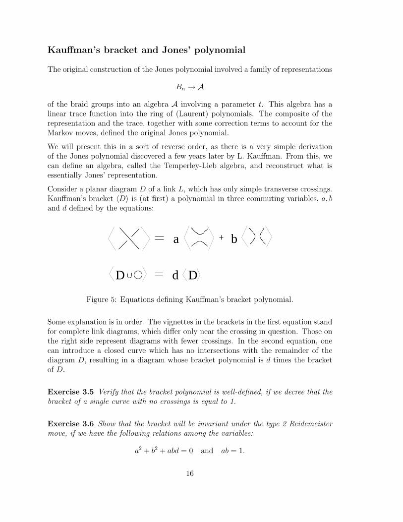
Consider a planar diagram D of a link L, which has only simple transverse crossings.Kauffman’s bracket 〈D〉 is (at first) a polynomial in three commuting variables, a, band d defined by the equations:

d D

ba

D

Figure 5: Equations defining Kauffman’s bracket polynomial.

Some explanation is in order. The vignettes in the brackets in the first equation standfor complete link diagrams, which differ only near the crossing in question. Those onthe right side represent diagrams with fewer crossings. In the second equation, onecan introduce a closed curve which has no intersections with the remainder of thediagram D, resulting in a diagram whose bracket polynomial is d times the bracketof D.

Exercise 3.5 Verify that the bracket polynomial is well-defined, if we decree that thebracket of a single curve with no crossings is equal to 1.

Exercise 3.6 Show that the bracket will be invariant under the type 2 Reidemeistermove, if we have the following relations among the variables:

a2 + b2 + abd = 0 and ab = 1.

16

Thus we make the substitutions b = a−1 and d = −a2 − a−2 and now consider thebracket to be a Laurent polynomial in the single variable a.

Exercise 3.7 Show that the invariance under the type 2 Reidemeister moves impliesthe bracket is invariant under the type 3 move, too.

Exercise 3.8 Calculate the bracket of the two trefoil knot diagrams with 3 crossings.Show that they are the same, except for reversal of the sign of the exponents.

Exercise 3.9 Investigate the effect of Reidemeister move 1 on the bracket of a di-agram, and show that it changes the bracket by a factor of −a±3, the sign of theexponent depending on the sense of the curl removed.

Because of this, one can define a polynomial invariant under all three Reidemeistermoves, by counting the number of positive minus the number of negative crossings,and modifying the bracket polynomial by an appropriate factor. A positive crossingcorresponds to a (positive) braid generator, if both strings are oriented from leftto right. This gives, up to change of variable, the Jones polynomial of the knot.Specifically, we define the writhe of an oriented diagram ~D for an oriented knot (or

link) ~K to be

w(D) =∑

c

εc

where the sum is over all crossings and εc = 1 if the crossing c is positive, and −1 ifnegative. Then we define

f ~K(a) = (−a3)−w( ~D)〈D〉.

This is an invariant of the oriented link ~K. If K happens to be a knot, it is independentof the orientation, as reorienting both strands of a crossing does not change its sign.It is related to the Jones polynomial VK(t) by a simple change of variables:

V ~K(t) = f ~K(t−1/4).

Exercise 3.10 Show that all exponents of a in 〈D〉 are divisible by 4 if D is a diagramof a knot (or link with an odd number of components). In other cases, they arecongruent to 2 mod 4. Thus the Jones polynomial is truly a (Laurent) polynomial int for knots and odd component links, but a polynomial in

√t in the other cases.

Representations

This is a very big subject, which I will just touch upon. By a representation ofa group we will mean a homomorphism of the group into a group of matrices, or

17

more generally into some other group, or ring or algebra. Often, but not always,we want the target to be finite-dimensional. We’ve already encountered the Artinrepresentation Bn → Aut(Fn), which is faithful. Here the target group is far frombeing “finite-dimensional.”

Another very important representation is the one defined by Jones [14] which gaverise to his famous knot polynomial, and the subsequent revolution in knot theory.The version I will discuss is more thoroughly described in [15]; it is based on theKauffman bracket, an elementary combinatorial approach to the Jones polynomial.First we need to describe the Temperley-Lieb Algebras Tn, in their geometric form.The elements of Tn are something like braids: we consider strings in a box, visualizedas a square in the plane, endpoints being exactly n specified points on each of the leftand right sides. The strings are not required to be monotone, or even to run acrossfrom one side to the other. There also may be closed components. Really what weare looking at are “tangle” diagrams. Two tangle diagrams are considered equal ifthere is a planar isotopy, fixed on the boundary of the square, taking one to the other.

��������

��������

��������

��������

��������

��������

��������

��������

��������

��������

��������

��������

��������

��������

��������

��������

��������

��������

��������

��������

Figure 6: A typical element in T5 and the generator e3.

Now we let A be a fixed complex number (regarded as a parameter), and formallydefine Tn to be the complex vector space with basis the set of all tangles, as describedabove, but modulo the following relations, which correspond to similar relations usedto define Kauffman’s bracket version of the Jones polynomial (we have promoted thevariable a to upper case).

= d K , d = -A -A2 -2

K

= A + A-1

Figure 7: Relations in Tn.

18

The first relation means that we can replace a tangle with a crossing by a linearcombination of two tangles with that crossing removed in two ways. As usual, thepictures mean that the tangles are identical outside the part pictured. The secondrelation means that we can remove any closed curve in the diagram, if it does nothave any crossings with the rest of the tangle, at the cost of multiplying the tangleby the scalar −A2 − A−2. Using the relations, we see that any element of Tn can beexpressed as a linear combination of tangles which have no crossings and no closedcurves – that is, disjoint planar arcs connecting the 2n points of the boundary. Thisgives a finite generating set, which (for generic values of A) can be shown to be a basisfor Tn as a vector space. But there is also a multiplication of Tn, a concatenation oftangles, in exactly the same way braids are multiplied. This enables us to considerTn to be generated as an algebra by the elements e1, . . . , en−1. In ei all the strings gostraight across, except those at level i and i + 1 which are connected by short caps;the generator e3 of T5 is illustrated in Figure 2. The identity of this algebra is simplythe diagram consisting of n horizontal lines (just like the identity braid). Tn canbe described abstractly as the associative algebra with the generators e1, . . . , en−1,subject to the relations:

eiej = ejei if |i− j| > 1 eiei±1ei = ei e2i = (−A2 − A−2)ei

It is an enjoyable exercise to verify these relations from the pictures. Now the Jonesrepresentation J : Bn → Tn can be described simply by considering a braid diagramas an element of the algebra. In terms of generators, this is just

J(σi) = A + A−1ei

The Burau representation

One of the classical representations of the braid groups is the Burau representation,which can be described as follows. Consider the definition of Bn as the mapping classgroup of the punctured disk Dn (Definition 4). As already noted, the fundamentalgroup of Dn is a free group, with generator xi represented by a loop, based at a pointon the boundary of the disk, which goes once around the ith puncture. Consider thesubgroup of π1(Dn) consisting of all words in the xi whose exponent sum is zero. Thisis a normal subgroup, and so defines a regular covering space

p : Dn → Dn.

The group of covering translations is infinite cyclic. Therefore, the homology H1(Dn)can be considered as a module over the polynomial ring Λ := Z[t, t−1], where trepresents the generator of the covering translation group. Similarly, if ∗ is a basepointof Dn, the relative homology group H1(Dn, p

−1(∗)) is a Λ-module.

19

A braid β can be represented as (an isotopy class of) a homeomorphism β : Dn → Dn

fixing the basepoint. This lifts to a homeomorphism β : Dn → Dn, which is unique ifwe insist that it fix some particular lift of the basepoint. The induced homomorphismon homology, β∗ : H1(Dn, p

−1(∗)) → H1(Dn, p−1(∗)) is a linear map of these finite-

dimensional modules, and so can be represented by a matrix with entries in Z[t, t−1].The mapping

β → β∗

is the Burau representation of Bn.

Let’s illustrate this for the case n = 3. D3 is replaced by the wedge of three circles,which is homotopy equivalent to it, to simplify visualization. The covering space Dn isshown as an infinite graph. Although as an abelian group H1(D3, p

−1(∗)) is infinitelygenerated, as a Λ-module it has three generators gi = xi, the lifts of the generatorsxi of D3, i = 1, 2, 3 beginning at some fixed basepoint in p−1(∗). The other elementsof H1(D3, p

−1(∗)) are represented by translates tngi.

Now consider the action of σ1 on D3, at the fundamental group level. As we saw inDefinition 5, σ1∗ takes x1 to x1x2x

−11 . Accordingly σ1∗ takes g1 to the lift of x1x2x

−11 ,

which is pictured in the lower part of the illustration. In terms of homology, this isg1 + tg2 − tg1. Therefore

σ1∗(g1) = (1− t)g1 + tg2.

Similarlyσ1∗(g2) = g1, σ1∗(g3) = g3.

3

......

x1

x2

x3

g1

g2

g3

p

t

tg

Figure 8: Illustrating the Burau representation for n = 3.

Exercise 3.11 Show that, with appropriate choice of basis, the Burau representationof Bn sends σj to the matrix

Ij−1 ⊕[

1− t t1 0

]⊕ In−j−1,

where Ik denotes the k × k identity matrix.

20

A probabilistic interpretation: Vaughan Jones offered the following interpretationof the Burau representation, which I will modify slightly because we have chosenopposite crossing conventions. Picture a braid as a system of trails. Wherever onetrail crosses under another there is a probability t that a person will jump from thelower trail to the upper trail; the probability of staying on the same trail is 1− t. Thei, j entry of the Burau matrix corresponding to a braid then represents the probabilitythat, if a person starts on the trail at level i, she will finish on the trail at level j.

It has been known for many years that this representation is faithful for n ≤ 3, andit is only within the last decade that it was found to be unfaithful for any n at all.John Moody [21] showed in 1993 that it is unfaithful for n ≥ 9. This has since beenimproved by Long and Paton [18] and more recently by Bigelow to n ≥ 5. The casen = 4 remains open, as far as I am aware.

Linearity of the braid groups.

It has long been questioned, whether the braid groups are linear, meaning that thereis a faithful representation Bn → GL(V ) for some finite dimensional vector space V .A candidate had been the so-called Burau representation, but as already mentionedit has been known for several years that Burau is unfaithful, in general.

The question was finally settled recently by Daan Krammer and Stephen Bigelow,using equivalent representations, but different methods. They use a representationdefined very much like the Burau representation. But instead of a covering of thepunctured disk Dn, they use a covering of the configuration space of pairs of pointsof Dn, upon which Bn also acts. This action induces a linear representation in thehomology of an appropriate covering, and provides just enough extra information togive a faithful representation!

Theorem 3.12 (Krammer [17], Bigelow [4]) The braid groups are linear.

In fact, Bigelow has announced that the BMW representation (Birman, Murakami,Wenzl) [6] is also faithful. Another open question is whether the Jones representationJ : Bn → Tn, discussed earlier, is faithful.

4 Ordering braid groups

This is, to me, one of the most exciting of the recent developments in braid theory.Call a group G right orderable if its elements can be given a strict total ordering <which is right-invariant:

∀x, y, z ∈ G, x < y ⇒ xz < yz.

21

Theorem 4.1 (Dehornoy[8]) Bn is right-orderable.

Interestingly, I know of three quite different proofs. The first is Dehornoy’s, thesecond is one that was discovered jointly by myself and four other topologists. Wewere trying to understand difficult technical aspects of Dehornoy’s argument, thencame up with quite a different way of looking at exactly the same ordering, but usingthe view of Bn as the mapping class group of the punctured disk Dn. Yet a thirdway is due to Thurston, using the fact that the universal cover of Dn embeds in thehyperbolic plane. Here are further details.

Dehornoy’s approach: It is routine to verify that a group G is right-orderable if andonly if there exists a subset Π (positive cone) of G satisfying:

(1) Π · Π = Π

(2) The identity element does not belong to Π, and for every g 6= 1 in G exactly oneof g ∈ Π or g−1 ∈ Π holds.

One defines the ordering by g < h iff hg−1 ∈ Π.

Exercise 4.2 Verify that the transitivity law holds, and that the ordering is right-invariant. Show that the ordering defined by this rule is also left-invariant if and onlyif gΠg−1 = Π for every g ∈ G; that is, Π is “normal.”

Dehornoy’s idea is to call a braid i-positive if it is expressible as a word in σj, j ≥ i insuch a manner that all the exponents of σi are positive. Then define the set Π ⊂ Bn

to be all braids which are i-positive for some i = 1, . . . , n − 1. To prove (1) above isquite easy, but (2) requires an extremely tricky argument.

Here is the point of view advocated in [11]. Consider Bn as acting on the complexplane, as described above. Our idea is to consider the image of the real axis β(R),under a mapping class β ∈ Bn. Of course there are choices here, but there is a unique“canonical form” in which (roughly speaking) R ∩ β(R) has the fewest number ofcomponents. Now declare a braid β to be positive if (going from left to right) thefirst departure of the canonical curve β(R) from R itself is into the upper half ofthe complex plane. Amazingly, this simple idea works, and gives exactly the sameordering as Dehornoy’s combinatorial definition.

Finally, Thurston’s idea for ordering Bn again uses the mapping class point of view,but a different way at looking at ordering a group. This approach, which has theadvantage of defining infinitely many right-orderings of Bn is described by H. Shortand B. Wiest in [27]. The Dehornoy ordering (which is discrete) occurs as one ofthese right-orderings – others constructed in this way are order-dense. A group Gacts on a set X (on the right) if the mapping x → xg satisfies: x(gh) = (xg)h andx1 = x. An action is effective if the only element of G which acts as the identity isthe identity 1 ∈ G. The following is a useful criterion for right-orderability:

22

Lemma 4.3 If the group G acts effectively on R by order-preserving homeomor-phisms, then G is right-orderable.

By way of a proof, consider a well-ordering of the real numbers. Define, for g andh ∈ G,

g < h ⇔ xg < xh at the first x ∈ R such that xg 6= xh.

It is routine to verify that this defines a right-invariant strict total ordering of G. (Bythe way, we could have used any ordered set in place of R.) For those wishing toavoid the axiom of choice (well-ordering R) we could have just used an ordering ofthe rational numbers.

The universal cover Dn of Dn can be embedded in the hyperbolic plane H2 in such away that the covering translations are isometries. This gives a hyperbolic structureon Dn. It also gives a beautiful tiling of H2, illustrated in Figure 9 for the case n = 2.

alpha in 0 2pi

D_n (here n=2)

universal cover

alpha in 0,2pi

D_n^ in H^2

infty

S^1

basecomp

gamma_alpha

tildegamma_alpha

Figure 9: The universal cover of a twice-punctured disk, with a lifted geodesic.(Courtesy of H. Short and B. Wiest [27]

Choose a basepoint ∗ ∈ ∂D and a specific lift ∗ ∈ H2. Now a braid is represented by ahomeomorphism of Dn, which fixes ∗. This homeomorphism lifts to a homeomorphism

23

of Dn, unique if we specify that it fixes ∗. In turn, this homeomorphism extends toa homeomorphism of the boundary of Dn But in fact, this homeomorphism fixes theinterval of ∂Dn containing ∗, and if we identify the complement of this interval withthe real line R, a braid defines a homeomorphism of R. This defines an action of Bn

upon R by order-preserving homeomorphisms, and hence a right-invariant orderingof Bn.

Two-sided invariance? Any right-invariant ordering of a group can be convertedto a left-invariant ordering, by comparing inverses of elements, but that ordering isin general different from the given one. We will say that a group G with strict totalordering < is fully-ordered, or bi-ordered, if

x < y ⇒ xz < yz and zx < zy,∀x, y, z ∈ G.

There are groups which are right-orderable but not bi-orderable – in fact the braidgroups!

Proposition 4.4 (N. Smythe) For n > 2 the braid group Bn cannot be bi-ordered.

The reason for this is that there exists a nontrivial element which is conjugate to itsinverse: take x = σ1σ

−12 and y = σ1σ2σ1 and note that yxy−1 = x−1. In a bi-ordered

group, if 1 < x then 1 < yxy−1 = x−1, contradicting the other conclusion x−1 < 1. Ifx < 1 a similar contradiction arises.

Exercise 4.5 Show that in a bi-ordered group g < h and g′ < h′ imply gg′ < hh′.Conclude that if gn = hn for some n 6= 0, then g = h. That is, roots are unique. Usethis to give an alternative proof that Bn is not bi-orderable if n ≥ 3.

Theorem 4.6 The pure braid groups Pn can be bi-ordered.

This theorem was first noticed by J. Zhu, and the argument appears in [25], based onthe result of Falk and Randall [13] that the pure braid groups are “residually torsion-free nilpotent.” Later, in joint work with Djun Kim, we discovered a really natural,and I think beautiful, way to define a bi-invariant ordering of Pn. We’ve already donehalf the work, by discussing Artin combing. Now we need to discuss ordering of freegroups.

Bi-ordering free groups

Lemma 4.7 For each n ≥ 1, the free group Fn has a bi-invariant ordering < withthe further property that it is invariant under any automorphism φ : Fn → Fn whichinduces the identity upon abelianization: φab = id : Zn → Zn.

24

The construction depends on the Magnus expansion of free groups into rings offormal power series. Let F be a free group with free generators x1, . . . , xn. LetZ[[X1, . . . , Xn]] denote the ring of formal power series in the non-commuting vari-ables X1, . . . , Xn.

Each term in a formal power series has a well-defined (total) degree, and we use O(d)to denote terms of degree ≥ d. The subset {1 + O(1)} is actually a multiplicativesubgroup of Z[[X1, . . . , Xn]]. Moreover, there is a multiplicative homomorphism

µ : F → Z[[X1, . . . , Xn]]

defined by

µ(xi) = 1 + Xi

µ(x−1i ) = 1−Xi + X2

i −X3i + · · ·

(2)

There is a very nice proof that µ is injective in [19], as well as discussion of some ifits properties. One such property is that commutators have zero linear terms. Forexample (dropping the µ)

[x1, x2] = x1x2x−11 x−1

2

= (1 + X1)(1 + X2)(1−X1 + X21 − · · · )(1−X2 + X2

2 − · · · )= 1 + X1X2 −X2X1 + O(3). (3)

Now there is a fairly obvious ordering of Z[[X1, . . . , Xn]]. Write a power series in as-cending degree, and within each degree list the monomials lexicographically accordingto subscripts). Given two series, order them according to the coefficient of the firstterm (when written in the standard form just described) at which they differ. Thus,for example, 1 and [x1, x2] first differ at the X1X2 term, and we see that 1 < [x1, x2].It is not difficult to verify that this ordering, restricted to the group {1 + O(1)} isinvariant under both left- and right-multiplication.

Exercise 4.8 Write x1, x2x1x−12 and x−1

2 x1x2 in increasing order, according to theordering just described.

Now we define an ordering of Pn. If α and β are pure n-braids, compare their Artincoordinates (as described earlier)

(α1, α2, . . . , αn−1) and (β1, β2, . . . , βn−1)

25

lexicographically, using within each Fk the Magnus ordering described above. This allneeds choices of conventions, for example, for generators of the free groups, describedin detail in [16]. The crucial fact is that the action associated with the semidirectproduct, by automorphisms ϕ, has the property mentioned in Lemma 4.7. We recallthe definition of a positive braid according to Garside: a braid is Garside-positiveif it can be expressed as a word in the standard generators σi with only positiveexponents.

Theorem 4.9 (Kim-Rolfsen) Pn has a bi-ordering with the property that Garside-positive pure braids are greater than the identity, and the set of all Garside-positivepure braids is well-ordered by the ordering.

Algebraic consequences: The orderability of the braid groups has implicationsbeyond what we already knew – e. g. that they are torsion-free. In the theory ofrepresentations of a group G, it is important to understand the group algebra CG andthe group ring ZG. These rings also play a role in the theory of Vassiliev invariants.A basic property of a ring would be whether it has (nontrivial) zero divisors. If agroup G has an element g of finite order, say gp = 1, but no smaller power of g is theidentity, then we can calculate in ZG

(1− g)(1 + g + g2 + · · ·+ gp−1) = 1− gp = 0

and we see that both terms of the left-hand side of the equation are (nonzero) divisorsof zero. A long-standing question of algebra is whether the group ring ZG can havezero divisors if G is torsion-free. We do know the answer for orderable groups:

Exercise 4.10 If R is a ring without zero divisors, and G is a right-orderable group,then the group ring RG has no zero divisors. Moreover, the only units of RG are themonomials rg, g ∈ G, r a unit of R.

Proposition 4.11 (Malcev, Neumann) If G has a bi-invariant ordering, then itsgroup ring ZG embeds in a division algebra, that is, an extension in which all nonzeroelements have inverses.

These results give us new information about the group rings of the braid groups.

Theorem 4.12 ZBn has no zero divisors. Moreover, ZPn embeds in a division alge-bra.

A proof of the theorem of Malcev and Neumann [20] can be found in [23].

Exercise 4.13 Which subgroups of Aut(Fn) are right-orderable?

26

Of course, Aut(Fn) itself is not right-orderable, because it has elements of finite order,e.g. permuting the generators.

A final note regarding orderings: As we’ve seen, the methods we’ve used for orderingBn and Pn are quite different. One might hope there could be compatible orderings:a bi-ordering of Pn which extends to a right-invariant ordering of Bn. But, in recentwork with Akbar Rhemtulla [24], we showed this is hopeless!

Theorem 4.14 (Rhemtulla, Rolfsen). For n ≥ 5, there is no right-invariantordering of Bn, which, upon restriction to Pn, is also left-invariant.

References

[1] E. Artin, Theorie der Zopfe, Abh. Math. Sem. Hamburg. Univ. 4(1926), 47 – 72.

[2] E. Artin, Theory of braids, Annals of Math. (2) 48(1947), 101 – 126.

[3] G. Baumslag, Automorphism groups of residually finite groups, J. London Math.Soc. 38(1963), 117–118.

[4] Bigelow, Stephen J. Braid groups are linear. J. Amer. Math. Soc. 14 (2001), no.2, 471–486 (electronic).

[5] J. Birman, Braids, links and mapping class groups, Annals of Math. Studies 82,Princeton Univ. Press, 1974.

[6] J. Birman and H. Wenzl, Braids, link polynomials and a new algebra, Trans.Amer. Math. Soc. 313(1989), 249 – 273.

[7] G. Burde and H. Zieschang, Knots, de Gruyter, 1985.

[8] P. Dehornoy, Braid groups and left distributive operations, Trans Amer. Math.Soc. 345(1994), 115 – 150.

[9] D. Epstein, J. Cannon, D. Holt, S. Levy, M. Paterson, W. Thurston, Wordprocessing in groups, Jones and Bartlett, 1992.

[10] R. Fenn, An elementary introduction to the theory of braids, notes by B. Gemein,1999, available at the author’s website.

[11] R. Fenn, M. Green, D. Rolfsen, C. Rourke, B. Wiest, Ordering the braid groups,Pacific J. Math. 191(1999), 49–74.

[12] E. Fadell and L. Neuwirth, Configuration spaces, Math. Scand. 10(1962), 111 –118.

27

[13] M. Falk and R. Randell, Pure braid groups and products of free groups, Braids(Santa Cruz 1986), Contemp. Math. 78 217–228.

[14] V. F. R. Jones, A polynomial invariant for knots via Von Neumann algebras,Bull. Amer. Math. Soc. 12(1985), 103–111.

[15] L. Kauffman, Knots and Physics, World Scientific, 1993.

[16] D. Kim and D. Rolfsen, An ordering for groups of pure braids and hyperplanearrangements, Canadian J. Math. 55(2002), 822-838.

[17] D. Krammer, The braid group B4 is linear. Invent. Math. 142 (2000), no. 3,451–486.

[18] D. Long and M. Paton, The Burau representation is not faithful for n ≥ 6,Topology 32(1993), 439 – 447.

[19] W. Magnus, A. Karrass and D. Solitar, Combinatorial group theory, Wiley 1966.

[20] A. I. Mal’cev, On the embedding of group algebras in division algebras, Dokl.Akad. Nauk SSSR 60 (1948) 1944-1501.

[21] J. Moody, The faithfulness question for the Burau representation, Proc. Amer.Math. Soc. 119(1993), 439 – 447.

[22] H. R. Morton, Threading knot diagrams. Math. Proc. Cambridge Philos. Soc. 99(1986), no. 2, 247–260.

[23] R. Mura and A. Rhemtulla, Orderable groups, Lecture Notes in Pure and AppliedMathematics, vol. 27, Marcel Dekker, New York, 1977.

[24] A Rhemtulla and D. Rolfsen, Local indicability in ordered groups: braids andelementary amenable groups, Proc. Amer. Math. Soc. 130(2002), 2569-2577 (elec-tronic).

[25] D. Rolfsen, J. Zhu, Braids, orderings and zero divisors, J. Knot Theory and itsRamifications 7(1998), 837-841.

[26] D. S. Passman, The algebraic structure of group rings, Pure and Applied Math-ematics, Wiley Interscience, 1977.

[27] H. Short and B. Wiest, Orderings of mapping class groups after Thurston,L’enseignement Mathmatique 46 (2000), 279-312.

28