Inspection of Earthen Embankment Dams Using Time Lapse ...

University of Mississippi University of Mississippi

eGrove eGrove

Electronic Theses and Dissertations Graduate School

2012

Inspection of Earthen Embankment Dams Using Time Lapse Inspection of Earthen Embankment Dams Using Time Lapse

Electrical Resistivity Tomography Electrical Resistivity Tomography

Jared Stewart Case

Follow this and additional works at: https://egrove.olemiss.edu/etd

Part of the Civil Engineering Commons

Recommended Citation Recommended Citation Case, Jared Stewart, "Inspection of Earthen Embankment Dams Using Time Lapse Electrical Resistivity Tomography" (2012). Electronic Theses and Dissertations. 77. https://egrove.olemiss.edu/etd/77

This Thesis is brought to you for free and open access by the Graduate School at eGrove. It has been accepted for inclusion in Electronic Theses and Dissertations by an authorized administrator of eGrove. For more information, please contact [email protected].

https://egrove.olemiss.edu/

https://egrove.olemiss.edu/etd

https://egrove.olemiss.edu/gradschool

https://egrove.olemiss.edu/etd?utm_source=egrove.olemiss.edu%2Fetd%2F77&utm_medium=PDF&utm_campaign=PDFCoverPages

http://network.bepress.com/hgg/discipline/252?utm_source=egrove.olemiss.edu%2Fetd%2F77&utm_medium=PDF&utm_campaign=PDFCoverPages

https://egrove.olemiss.edu/etd/77?utm_source=egrove.olemiss.edu%2Fetd%2F77&utm_medium=PDF&utm_campaign=PDFCoverPages

mailto:[email protected]

INSPECTION OF EARTHEN EMBANKMENT DAMS USING TIME LAPSE ELECTRICAL

RESISTIVITY TOMOGRAPHY

A Thesis

presented in partial fulfillment of requirements

for the degree of Master of Science

in the Department of Civil Engineering

The University of Mississippi

by

JARED S. CASE

MAY 2012

Copyright Jared S. Case 2012

ALL RIGHTS RESERVED

ii

ABSTRACT

According to the National Inventory of Dams (NID), the number of dams across the

United States is approximately 85,000. Many of these dams are more than 50 years old and need

vast attention to ensure their safety. It is difficult to obtain a full assessment of the dam just by

visual inspections alone. This is because many problems associated with dam failure occur

internally, which makes it difficult to be observed by the dam inspectors. Examples of these

flaws are piping and seepage (flow of water through or around dam walls). It is in this area

where geophysical methods can aid in obtaining a more confident evaluation of a dam’s

integrity. Electrical resistivity is one geophysical technique that would be useful in detecting

internal flaws associated with seepage and piping because it is sensitive to moisture changes. A

study is being conducted to examine the feasibility of electrical resistivity tomography (ERT) to

map and monitor internal compromised zones within earthen embankment dams. Two quarter-

scaled earthen embankment dams were built at the United States Department of Agriculture

(USDA) Agriculture Research Service (ARS) Hydraulics and Engineering Research Unit

(HERU) in Stillwater, Oklahoma. These two dams were constructed with known internal

compromised zones that are susceptible to seepage and piping. Electrical resistivity surveys were

conducted on the completed dams using a 56 electrode dipole-dipole array. The collected data

was then processed using electrical resistivity tomography (ERT) imaging software and evidence

of these two compromised zones was easily visible. Also, additional surveys were conducted in

order to monitor the changes in electrical signatures associated with changes in these zones due

to filling of the reservoir and environmental/climate changes.

iii

DEDICATION

This thesis is dedicated to my family and friends who believed in me and stood by me for

the two years. This strong support system is who I thank for helping and guiding me along

during this time. Last but not least, I want to thank God who without, none of this would be

possible.

iv

LIST OF ABBREVIATION AND SYMBOLS

2D Two dimensional

A Cross sectional area

Tortuosity coefficient

AGI Advanced Geosciences Inc.

ARS Agricultural Research Service

ASDSO Association of State Dam Safety Officials

Equivalent conductance of the counterions as a function of pore fluid

Clay content

Clay fraction conductivity

CEC Cation exchanged capacity

Bulk conductivity

CST Constant separation traversing

Partially saturated shaley sand conductivity

Pore water conductivity

v

d Depth of penetration of electrical resistivity survey

EM Electromagnetics

ERT Electrical resistivity tomography

ES Electrode spacing

ES Electrical sounding

Formation factor of clean sand

Formation factor of shaley sand

Geometric factor, function of porosity, water saturation level, and pore geometry

HERU Hydraulic Engineering Research Unit

Current

Current density

Electrode configuration geometric factor

Length

LL Liquid limit

Cementation exponent

vi

Saturation exponent

NCPA National Center for Physical Acoustics

NID National Inventory of Dams

PI Plasticity index

Concentration of sodium exchange cations associated with clay

R Resistance

Res Reservoir

Radial distance from point source electrode

RMS Root mean square

Degree of saturation

SERRI Southeastern Region Research Initiative

Spread Length

SP Self-potential

TDR Time domain reflectometer

USDA United States Department of Agriculture

vii

USGS United States Geological Survey

V Voltage

Total volume

Pore (void) space volume

Pore water volume

VES Vertical electrical sounding

Change in voltage

Maximum equivalent ionic conductance of sodium exchange ions

Electrical resistivity

Apparent resistivity

Bulk resistivity

Mineral grain density

Pore water resistivity

Electrical conductivity

Porosity

viii

ACKNOWLEDGEMENTS

I would like to first acknowledge my thesis advisor Dr. Craig Hickey, Senior Research

Scientist at NCPA, Associate Professor of Geology and Geological Engineering, for all of this

help, guidance, and support while obtaining my graduate degree. It was he who gave me all the

tools in order to develop an understanding for geophysics and the ability to apply what I have

learned towards the research. He has helped me grow as an individual and as a professional in

the field of geophysics and engineering.

Also I would like to thank my academic advisor, Dr. Chung Song, Associate Professor of

Civil Engineering, for giving me the opportunity to advance my education here at the University

of Mississippi. Whether it was through classroom lectures or office hour visits, I was able to gain

the knowledge needed to expand my engineering skills.

I would also like to thank my committee member Dr. Elizabeth Ervin, Assistant Professor

of Civil Engineering, for agreeing to be on my thesis committee on short notice.

I would like to a thank you to my colleagues Leti Wodajo and Binyam Tadese for their

help with data collection.

A special thanks needs to be given to Dr. Greg Hanson and the USDA-ARS Hydraulic

Engineering Research Unit team for their assistance during out visits to the research facility.

ix

This work was funded by the Department of Homeland Security-sponsored Southeastern

Region Research Initiative (SERRI) at the Department of Energy’s Oak Ridge National

Laboratory Award # DE-AC05-00OR22725 Geophysical Signatures of Compromised Zones

within Earthen Embankments and Levees. This material is based upon work supported by the

U.S. Department of Homeland Security under U.S. Department of Energy Interagency

Agreement 43WT10301. The views and conclusions contained in this document are those of the

authors and should not be interpreted as necessarily representing the official policies, either

expressed or implied, of the U.S. Department of Homeland Security.

x

TABLE OF CONTENTS

Abstract --------------------------------------------------------------------------------------------------------- ii

Dedication ----------------------------------------------------------------------------------------------------- iii

List of abbreviations and symbols --------------------------------------------------------------------------iv

Acknowledgements ----------------------------------------------------------------------------------------- viii

List of tables-------------------------------------------------------------------------------------------------- xiv

List of figures ------------------------------------------------------------------------------------------------- xv

1. Introduction ------------------------------------------------------------------------------------------------- 1

1.1 Introduction to dams ------------------------------------------------------------------------------- 1

1.2 Failure of dams ------------------------------------------------------------------------------------- 3

1.3 Previous work using electrical resistivity tomography --------------------------------------- 4

1.4 Motivation of research ---------------------------------------------------------------------------- 6

2. Electrical Resistivity --------------------------------------------------------------------------------------- 8

2.1 Introduction ----------------------------------------------------------------------------------------- 8

2.2 Resistivity theory----------------------------------------------------------------------------------- 8

2.3 Soil physics ----------------------------------------------------------------------------------------- 9

xi

2.3.1 Effect of porosity and saturation of resistivity ----------------------------------------- 12

2.3.2 Effect of clay content on resistivity ----------------------------------------------------- 19

2.4 Summary ------------------------------------------------------------------------------------------- 25

3. Electrical Surveys ----------------------------------------------------------------------------------------- 26

3.1 Introduction ----------------------------------------------------------------------------------------------- 26

3.2 Point source electrode ---------------------------------------------------------------------------- 26

3.3 Electrode configurations ------------------------------------------------------------------------- 29

3.4 Electrical resistivity surveys --------------------------------------------------------------------- 31

3.5 Building an apparent resistivity pseudosection ----------------------------------------------- 32

3.6 ERT inversion ------------------------------------------------------------------------------------- 36

3.7 Electrode configuration selection --------------------------------------------------------------- 37

3.8 Summary ------------------------------------------------------------------------------------------- 40

4. Forward Modeling ---------------------------------------------------------------------------------------- 41

4.1 Introduction ---------------------------------------------------------------------------------------- 41

4.2 Forward modeling using EarthImager 2D ----------------------------------------------------- 41

xiii

4.3 Zone detection ------------------------------------------------------------------------------------- 42

4.4 Zone resolution ------------------------------------------------------------------------------------ 48

4.5 Summary ------------------------------------------------------------------------------------------- 51

5. Field measurements and discussion of results--------------------------------------------------------- 53

5.1 Introduction ---------------------------------------------------------------------------------------- 53

5.2 Description of embankment dam --------------------------------------------------------------- 53

5.3 Electrical resistivity equipment and acquisition ---------------------------------------------- 59

5.4 Schedule of surveys ------------------------------------------------------------------------------- 65

5.5 Discussion of results ------------------------------------------------------------------------------ 65

5.5.1 Results from in situ sensors --------------------------------------------------------------- 66

5.5.2 ERT tomogram results related to environmental changes ---------------------------- 71

5.5.3 ERT tomograms related to cyclic loading of the reservoir --------------------------- 77

5.6 Summary ------------------------------------------------------------------------------------------- 90

6. Conclusions ------------------------------------------------------------------------------------------------ 92

Bibliography -------------------------------------------------------------------------------------------------- 96

xiii

Appendix 1 ---------------------------------------------------------------------------------------------------- 99

Vita ----------------------------------------------------------------------------------------------------------- 102

xiv

LIST OF TABLES

2.1 Cation exchange capacity of common clays ------------------------------------------------------ 21

3.1 Pros and cons of common electrode configurations --------------------------------------------- 30

5.1 Lift information for experimental embankment dam -------------------------------------------- 55

5.2 Sieve analysis on embankment soils --------------------------------------------------------------- 58

5.3 List of equipment used for ERT surveys ---------------------------------------------------------- 60

5.4 Resistivity meter parameters ----------------------------------------------------------------------- 64

A.1 Schedule for surveys conducted on embankment dam ---------------------------------------- 101

xv

LIST OF FIGURES

1.1 Distribution of dams across United States by height (NID, 2009) ----------------------------- 2

1.2 Types of dam designs (NID, 2009) ----------------------------------------------------------------- 2

1.3 Dam failure causes (Department of Ecology for the State of Washington, 2007) ----------- 3

1.4 United States dam failures (ASDSO, 2009) ------------------------------------------------------ 4

2.1 Measuring resistance across a block of material -------------------------------------------------- 9

2.2 Resistivity of various geological materials (Palacky, 1987) - ---------------------------------- 10

2.3 Archie’s First Law,

Sw 1 -------------------------------------------------------------------------- 13

2.4 Archie’s Second Law varying cementation exponent ( = 0.32, = 1, = 2) --------- 14



2.7 Archie’s Second Law varying tortuosity coefficient ( = 0.32, = 2, = 2) ---------- 16



2.10 Archie’s Second Law varying saturation exponent ( = 0.32, = 2, = 1) ----------- 18

xvi



2.13 Waxman Smits equation varying clay type ( = 0.36, = 2, = 1) ---------------------- 23

2.14 Waxman Smits equation varying clay percentage ( = 0.36, = 2, = 1) -------------- 24

3.1 Point source electrode -------------------------------------------------------------------------------- 27

3.2 Four electrode setup ---------------------------------------------------------------------------------- 28

3.3 Wenner electrode configuration -------------------------------------------------------------------- 30

3.4 Schlumberger electrode configuration ------------------------------------------------------------- 31

3.5 Dipole-dipole electrode configuration ------------------------------------------------------------- 31

3.6 Dipole-dipole electrode configuration used to illustrate the location of measured

apparent resistivity (each circle represents 1 apparent resistivity measurement) ----------- 33

3.7 Apparent resistivity pseudosections for initial survey on embankment using

(a) Wenner array, (b) Schlumberger array, and (c) dipole-dipole array ---------------------- 35

3.8 Example of output from EarthImager 2D, (a) measured apparent

resistivity pseudosection, (b) calculated apparent resistivity pseudosection,

and (c) inverted resistivity section for survey conducted on embankment

dam using a dipole-dipole configuration with electrode spacing equal to 0.5

feet ------------------------------------------------------------------------------------------------------ 37

3.9 Resistivity tomogram for initial survey on embankment using

(a) Wenner array, (b) Schlumberger array, and (c) dipole-dipole array ---------------------- 39

xvii

4.1 Synthetic model created to study the dependence on zone size for zone

size. The zone resistivity is ½ the background resistivity and is placed at a

depth of 4.5 electrode spacing ---------------------------------------------------------------------- 43

4.2 Resistivity tomogram for zone size equal to 1 ES x 1 ES -------------------------------------- 43



4.5 Synthetic model created for analysis of sensitivity to contrast variation.

Zone dimensions are 3 ES x 3 ES. Zone is placed at a depth of 3 electrode

spacing ------------------------------------------------------------------------------------------------- 45

4.6 Resistivity tomogram with contrast of 1.14:1 (200 ohm*m to 175 ohm*m) ---------------- 45

4.7 Resistivity tomogram with contrast of 1.33:1 (200 ohm*m to 150 ohm*m) ---------------- 46

4.8 Resistivity tomogram with contrast of 2:1 (200 ohm*m to 100 ohm*m) -------------------- 46

4.9 Resistivity tomogram with contrast of 0.89:1 (200 ohm*m to 225 ohm *m ----------------- 47

4.10 Resistivity tomogram with contrast of 0.8:1 (200 ohm*m to 250 ohm *m) ----------------- 47

4.11 Resistivity tomogram with contrast of 0.67:1 (200 ohm*m to 300 ohm*m) - --------------- 47

4.12 Synthetic model created for separation variation, zone dimensions are

3 ES x 3 ES and is placed at a depth of 3 ES ----------------------------------------------------- 48

4.13 Resistivity tomogram with separation of 1 ES between zones --------------------------------- 49

xviii

4.14 -Resistivity tomogram with separation of 2 ES between zones --------------------------------- 49

4.15 -Resistivity tomogram with separation of 3 ES between zones --------------------------------- 49

4.16 -Resistivity tomogram with a random noise level of 1 % --------------------------------------- 50



5.1 ---Schematic of embankment's geometry ------------------------------------------------------------ 54

5.2 ---Plan view of embankment dam --------------------------------------------------------------------- 57

5.3 ---Sensor pack locations within dam ------------------------------------------------------------------ 59

5.4 ---SuperStingTM

R8 resistivity meter ----------------------------------------------------------------- 61

5.5 ---Switch box- -------------------------------------------------------------------------------------------- 62

5.6 ---Electrode stakes and switches ---------------------------------------------------------------------- 62

5.7 ---Field setup of ERT equipment ---------------------------------------------------------------------- 63

5.8 ---Moisture content plot for embankment (lateral variation) ------------------------------------ 68

5.9 ---Moisture content plot for embankment (vertical variation) ----------------------------------- 69

5.10 -Temperature plot for embankment (lateral variation) ----------------------------------------- 70

xix

5.11 Temperature plot for embankment (vertical variation) ---------------------------------------- 71

5.12 Electrical resistivity tomogram for survey conducted October 13, 2011

at 15:45. Reservoir is empty ----------------------------------------------------------------------- 72

5.13 Electrical resistivity tomogram for survey conducted November 29, 2011

at 11:30. Reservoir is empty. ----------------------------------------------------------------------- 73

5.14 Electrical resistivity tomogram for survey conducted March 14, 2011

at 9:40. Reservoir has been empty since December 6, 2010. ---------------------------------- 74

5.15 Electrical resistivity tomography for survey conducted May 23, 2011

at 10:45. Reservoir has been emptied since March 16, 2011. --------------------------------- 75

5.16 Electrical resistivity tomogram for survey conducted August 1, 2011

at 12:45. Reservoir has been emptied since May 27, 2011. ----------------------------------- 76

5.17 Survey conducted on dam with a full reservoir -------------------------------------------------- 77


at 11:30. Reservoir is empty. ----------------------------------------------------------------------- 78


at 10:45. Reservoir is full for 18 hrs. -------------------------------------------------------------- 79

5.20 Electrical resistivity tomogram for survey conducted December 1, 2010

at 1300. Reservoir is full for 44 hrs. -------------------------------------------------------------- 79


at 10:40. Reservoir has been drained. Draining process took 19.5 hours. ------------------- 80


at 13:45. Reservoir has been filled for the second loading for 0 hrs. ------------------------- 81

5.23 Visible evidence of seepage through embankment ---------------------------------------------- 81


at 9:40. Reservoir has been empty since December 6, 2010. ---------------------------------- 83

xx


at 14:40. Reservoir filled for 1 hr. ----------------------------------------------------------------- 83


at 10:30. Reservoir has been filled for 21 hrs. --------------------------------------------------- 83


at 10:25. Reservoir has been filled for 44.5 hrs. ------------------------------------------------- 84

5.28 Electrical resistivity tomography for survey conducted May 23, 2011

at 10:45. Reservoir has been emptied since March 16, 2011. --------------------------------- 85

5.29 Electrical resistivity tomogram for survey conducted May 24, 2011

at 9:35. Reservoir has been filled for 20.5 hrs. -------------------------------------------------- 86


at 7:40. Reservoir has been filled for 43 hrs. ---------------------------------------------------- 86


at 6:10. Reservoir has been filled for 89 hrs. ---------------------------------------------------- 86

5.32 Cracking of embankment ---------------------------------------------------------------------------- 87


at 12:45. Reservoir has been emptied since May 27, 2011. ---------------------------------- 89


at 7:45. Reservoir was filled to a height of 1.5 feet. ------------------------------------------- 89


at 11:45. Reservoir was filled to a height of 2.6 feet. ------------------------------------------ 89


at 14:00. Reservoir was filled to a height of 3.2 ft. -------------------------------------------- 90

1

1. INTRODUCTION

1.1 Introduction to dams

A dam is a water retaining barrier; ultimately designed to restrict the flow of water into

specific regions. Concrete (arch/gravity) and earthen embankments are two common types of

dams, each one having a unique structural design in order to hold back the massive amount of

water. These structures are built mainly out of concrete (arch/ gravity) or using a mixture of clay,

sand, and rock (earthen embankments). Applications of dams include electrical generation

(produce hydropower), flood control (prevent flooding downstream of dam due to heavy

rainfall), irrigation (watering of crops using reservoir water), water supply (drinking water

gained from dam’s reservoir), recreation (boating/ skiing), etc. The numerous functions these

dams possess show how important they are to the national infrastructure. The National Inventory

of Dams (NID) is an Army Corps of Engineers website that contains information about the dams

located across the United States (US). According to this database there are currently over 85,000

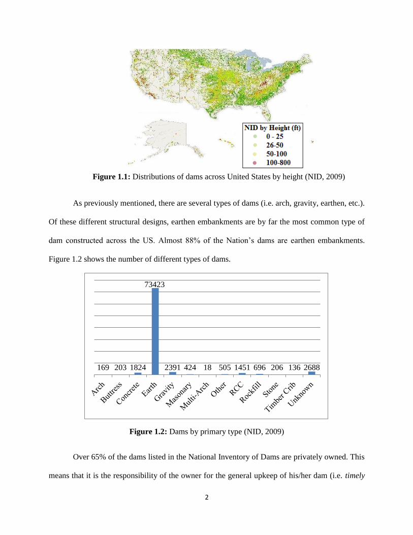
dams across the US. The distribution of these dams is shown in Figure 1.1. According to the

National Inventory of Dams (NID), 2009 database, approximately 28,000 dams were constructed

before the year 1960. This makes about 28,000 dams 50 years or older. Since the life of these

structures was originally designed to be 50 years, vast investigating and monitoring needs to be

conducted in order to maintain their integrity and/or to make necessary repairs to the dam.

2

Figure 1.1: Distributions of dams across United States by height (NID, 2009)

As previously mentioned, there are several types of dams (i.e. arch, gravity, earthen, etc.).

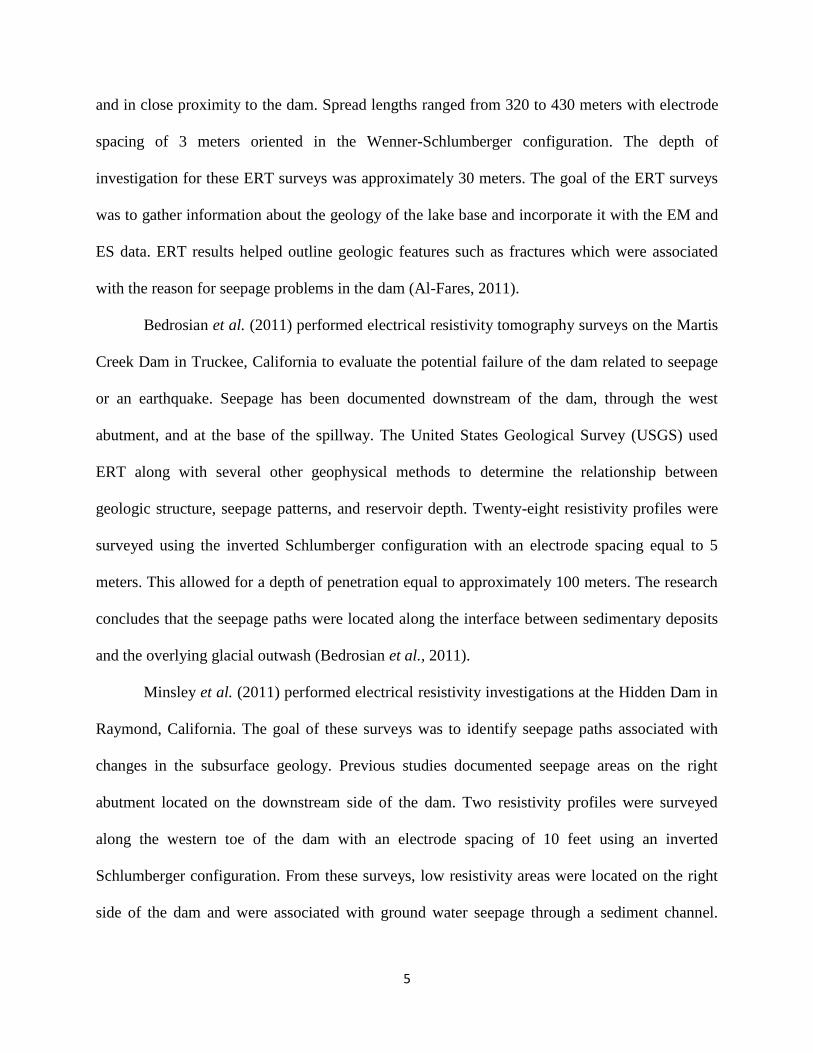
Of these different structural designs, earthen embankments are by far the most common type of

dam constructed across the US. Almost 88% of the Nation’s dams are earthen embankments.

Figure 1.2 shows the number of different types of dams.

Figure 1.2: Dams by primary type (NID, 2009)

Over 65% of the dams listed in the National Inventory of Dams are privately owned. This

means that it is the responsibility of the owner for the general upkeep of his/her dam (i.e. timely

169 203 1824

73423

2391 424 18 505 1451 696 206 136 2688

3

investigations, maintenance, repairs, etc). The general upkeep of these privately owned dams as

well as those run by local, state, and federal agencies is necessary to protect lives and

economical/environmental needs in the downstream area.

1.2 Failure of dams

The Department of Ecology for the State of Washington organizes the cause of dam failures

into four main categories. The pie chart in Figure 1.3 indicates that the leading cause of dam

failure is caused by overtopping (34 % of all failures nationally). Overtopping can be related to

poor spillway design, blockage of spillway by debris, and also possible settlement of the dam

crest. The next most common cause of failure is foundation defects (30% of all failures

nationally) which may be due to differential settlement, slope instability, high uplift pressures,

and uncontrollable seepage in the foundation. The third most common cause of failure is seepage

and piping (20% of all failures nationally). Failure from seepage/piping is related to internal

erosion due to the flow of water through the dam body, along conduits and valves, or through

burrows created by animals. The fourth common failure listed by the Department of Ecology for

the State of Washington is by conduits and valves (10% of all failures nationally). These failures

are caused by embankment material being washed into the conduit through joints or cracks. The

remaining 6% of all national failures are undetermined.

Figure 1.3: Dam failure causes (Department of Ecology for the State of Washington, 2007)

34%

30%

20%

10% 6%

Overtopping

Foundation Defects

Piping Seepage

Conduits/Valves

Other

4

Failure of embankments brings great economic and environmental damage to its

surroundings. As these structures continue to age and the downstream population increases, the

potential for catastrophic failure and its impact continues to grow. According to the Association

of State Dam Safety Officials (ASDSO), 132 failures and 434 “incidents” have occurred from

January 2005 to January 2009. These “incidents” would likely have resulted in dam failure

without proper remedial actions. Figure 1.4 is a non-comprehensive map created from a

compiled list of ASDSO reported dam failures. The figure shows the approximate location of

these failures, the years they occurred, and the related casualties.

Figure 1.4: United States dam failures (ASDSO, 2009)

1.3 Previous work using electrical resistivity tomography

Al-Fares (2011) conducted electrical resistivity tomography surveys to characterize water

leakage along the Afamia B dam in Syria. Other geophysical methods that were used include

electromagnetic (EM) and electrical sounding (ES). Five resistivity surveys were conducted, the

first three were perpendicular to the main valley, and the last two were parallel to the main valley

5

and in close proximity to the dam. Spread lengths ranged from 320 to 430 meters with electrode

spacing of 3 meters oriented in the Wenner-Schlumberger configuration. The depth of

investigation for these ERT surveys was approximately 30 meters. The goal of the ERT surveys

was to gather information about the geology of the lake base and incorporate it with the EM and

ES data. ERT results helped outline geologic features such as fractures which were associated

with the reason for seepage problems in the dam (Al-Fares, 2011).

Bedrosian et al. (2011) performed electrical resistivity tomography surveys on the Martis

Creek Dam in Truckee, California to evaluate the potential failure of the dam related to seepage

or an earthquake. Seepage has been documented downstream of the dam, through the west

abutment, and at the base of the spillway. The United States Geological Survey (USGS) used

ERT along with several other geophysical methods to determine the relationship between

geologic structure, seepage patterns, and reservoir depth. Twenty-eight resistivity profiles were

surveyed using the inverted Schlumberger configuration with an electrode spacing equal to 5

meters. This allowed for a depth of penetration equal to approximately 100 meters. The research

concludes that the seepage paths were located along the interface between sedimentary deposits

and the overlying glacial outwash (Bedrosian et al., 2011).

Minsley et al. (2011) performed electrical resistivity investigations at the Hidden Dam in

Raymond, California. The goal of these surveys was to identify seepage paths associated with

changes in the subsurface geology. Previous studies documented seepage areas on the right

abutment located on the downstream side of the dam. Two resistivity profiles were surveyed

along the western toe of the dam with an electrode spacing of 10 feet using an inverted

Schlumberger configuration. From these surveys, low resistivity areas were located on the right

side of the dam and were associated with ground water seepage through a sediment channel.

6

These interpretations agreed with self-potential (SP) measurements on the Hidden Dam site

(Minsley et al., 2011).

Weller et al. (2005) performed several resistivity surveys on a series of dikes located in

North Vietnam along the Red River. This system of dikes is a vital infrastructure to the province

of Thai Binh and protects the province from flooding during monsoon seasons. Currently water

leakage is occurring through the dike caused by termites digging their nest into the dike. The

objective of the electrical surveys was to locate these defects in the dikes. Several surveys were

conducted using a half-Wenner electrode configuration. This research was able to verify that

imaging termite nests in the dikes was possible. The nests show up as a high resistivity and can

be resolved in the data set using an electrode spacing of 1 meter (Weller et al., 2005).

1.4 Motivation of research

Since the majority of the dams across the United States are approaching their design life of

50 years, vast attention and concern needs to be aimed at them to assure their safety. The dam’s

integrity and the safety of the population downstream ultimately depend on timely visual

inspections and appropriate remedial actions on the embankment. Visual inspection for assessing

a dam’s performance is greatly hindered by only providing information regarding problems

observed from the surface. For instance, seepage (flow of water through, under, or around dam

walls) is a major source for earthen embankment failures and usually cannot be detected by

visual inspections until the process has progressed to an advanced stage. By this time, it is

possible that the integrity of the dam may already be compromised.

It is in this area where electrical resistivity tomography (ERT), a non-invasive

geophysical technique, can aid visual inspections in gaining a more complete understanding of

the dam’s integrity. Since ERT is sensitive to changes in moisture, it is useful for detecting

7

seepage water through a dam before it develops to an advanced stage. ERT can give vital

information about the integrity of the interior of the dam that a visual inspection cannot do.

In this research project, two quarter-scaled experimental earthen embankment dams were

constructed at the Agricultural Research Service, Hydraulic Engineering Research Unit in

Stillwater, Oklahoma. These dams were constructed with two known anomalous zones that

would be susceptible to seepage and piping. Time lapse ERT surveys were performed on the

scaled embankments through a series of scheduled trips to the research site. Data gained from

these trips was used to determine how seasonal and climate variations as well as cyclic loading

of the reservoir affect the changes in the electrical signatures of these anomalous zones.

The objective of this research is to use electrical resistivity tomography as a tool in order to

map and locate zones within an earthen embankment dam that would be susceptible to seepage

and piping. The second research objective is to determine the optimal time to perform these ERT

surveys. More specifically, the goal is to determine the environmental conditions and the

physical state of the dam (saturated/ dry) in which the compromised zones produce the largest

anomalies within the data set.

8

2. ELECTRICAL RESISTIVITY

2.1 Introduction

The third most common cause of dam failure is seepage, which may not be noticeable

during a visual inspection until it has progressed to a more advanced or threatening stage.

Electrical resistivity tomography, a non-destructive geophysical method, can aid visual

inspection in the evaluation of the performance of an embankment dam. This method will assist

in evaluating a dam for seepage because of its sensitivity to changes in moisture, ultimately

providing additional information regarding the internal integrity of the structure.

The electrical resistivity method is used to study the distribution of electrical properties in

the subsurface by injecting electrical current and measuring the reduced induced potential at

various locations along the ground surface. These variations in electrical resistivity are used to

map vertical and horizontal discontinuities within the area of interest (Kearey and Brooks, 1984).

Areas where electrical resistivity tomography is used include: investigation of dams and levees,

detection of caverns/tunnels, mapping contamination plumes, locating ground water aquifers,

determining depth to bedrock, etc (Advanced Geosciences Inc., agiusa.com).

2.2 Resistivity theory

Resistivity is a material property defining how strongly a material opposes the flow of

electrical current. Mathematically, the resistivity of a given cube of soil can be defined as

(

) (2.1)

9

where the resistivity (ohm*m) of a given material is equal to the resistance R (ohms) of the

cube of material times the ratio of cross sectional area A (m2) to the length L (m) of the material.

The electrical resistance (R) of the material is described using Ohm’s Law

(2.2)

where V (volts) is the potential difference across the cube of material and I (Amperes) is the

electrical current injected. Figure 2.1 describes the parameters used in determining the resistivity

of a simple block of material. If the injected current and the geometrical parameters (A and L) are

known, and the potential difference is measured across the body of material, the resistivity can

easily be calculated.

Figure 2.1: Measuring resistance across a block of material

The inverse of electrical resistivity is the electrical conductivity, , with units of (Siemens/meter

or mho/meter) and is also commonly used to describe the electrical properties of soils. Resistivity

is a characteristic electrical material property and varies from one soil to the next.

2.3 Soil physics

ΔV

A

L I

R

10

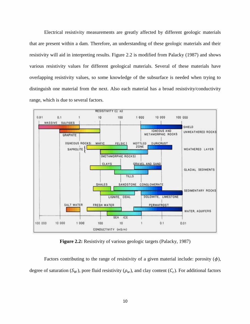
Electrical resistivity measurements are greatly affected by different geologic materials

that are present within a dam. Therefore, an understanding of these geologic materials and their

resistivity will aid in interpreting results. Figure 2.2 is modified from Palacky (1987) and shows

various resistivity values for different geological materials. Several of these materials have

overlapping resistivity values, so some knowledge of the subsurface is needed when trying to

distinguish one material from the next. Also each material has a broad resistivity/conductivity

range, which is due to several factors.

Figure 2.2: Resistivity of various geologic targets (Palacky, 1987)

Factors contributing to the range of resistivity of a given material include: porosity ( ),

degree of saturation ( ), pore fluid resistivity ( ), and clay content ( ). For additional factors

11

affecting the resistivity of geological materials see Freidman (2005). Porosity, ( ), is measure of

the void spaces in a material and is expressed by

(2.3)

where Vv is the volume of pore space and VT is the total volume of the material.

The degree of saturation, ( ), is a measurement of the volume of moisture in a soil. The degree

of saturation is the ratio of the volume of water (Vw) to volume of void space (Vv) and is given by

. (2.4)

The resistivity of the fluid in the pore space of a soil is known as the pore fluid resistivity

(w). The resistivity of the pore fluid can be easily measured for an extracted fluid sample using

a handheld resistivity meter. The clay fraction or clay content is the percentage of clay within the

soil. There is some ambiguity in the definition of clay. Clay can be defined as materials having a

grain size less than 2m or a group of hydrous aluminum Phyllosilicates minerals which include

Kaolinite, Montmorillonite-smectite, Illite, and Chlorite. The clay fraction defined by grain size

is determined from a sieve analysis. An X-ray diffraction test determines the clay fraction based

upon the mineralogy of the material and not the particle size. Since clays carry an electric charge,

the presence of this material will affect resistivity measurements.

An understanding of these properties and how they ultimately affect the measured

resistivity of soils during seepage and piping is very important. Seepage is the process of water

infiltrating through the dam walls and into the core of the dam (area of interest during electrical

resistivity surveys). The presence of water will cause an increase in the saturation level resulting

in a decrease in the measured resistivity. The removal of fines from the dam occurs during

piping. The resistivity measured during this process will be driven by the competing factor of

12

increasing porosity and decreasing clay content. Increasing porosity causes a decrease in

resistivity while a decrease in clay content leads to an increase in resistivity. One goal of this

research is to investigate the change in electrical resistivity in a scaled embankment during active

seepage and piping.

2.3.1 Effects of porosity and saturation on resistivity

Archie’s first law is an empirical formula relating the formation factor to the porosity of a

fully saturated rock (i.e. clean sand or coarse grained material). Archie’s first law is expressed as

. (2.5)

The bulk resistivity ( ) of a material is calculated knowing the resistivity of the pore fluid ( ),

porosity of the sand ( ), and the cementation exponent ( ). The ratio of the bulk resistivity to

the pore fluid resistivity is known as the formation factor ,

(2.6)

For sand, the porosity typically ranges from 0.3 to 0.45, and the cementation exponent ranges

from 1.3 to 2.5 for rocks and 1.8 to 2 for sands. Figure 2.3 illustrates the predicted resistivity

using Archie’s first law. A typical range of porosity for sand is plotted on the x-axis and the

calculated formation factor is plotted on the y-axis. Each line represents a chosen cementation

exponent that falls within the range for coarse grained and sandy materials. The graph shows that

when the porosity of a fully saturated material increases, the resistivity of the material decreases.

This is because when the porosity increases, the amount of water the soil can hold increases,

allowing better conduction of electrical current. Also, the formation factor is more sensitive to

the range of cementation exponents at low porosities, but as porosities increase the selection of

the cementation exponents play less of a role.

13

Figure 2.3: Archie’s First Law,

Sw 1

Archie’s first law assumes that the material is fully saturated,

Sw 1. Archie’s second law

introduces a saturation term in order to calculate the bulk resistivity of partially saturated sand,

(2.7)

The bulk resistivity ( ) can be calculated knowing the resistivity of the pore fluid ( ),

tortuosity ( ), an empirical constant typically set to 1, porosity ( ) of the material, the

cementation exponent ( ), degree of saturation ( ), and the saturation exponent , an

empirical coefficient that depends on the pore fluid, but is typically set to 2 when the pore fluid

of interest is water.

Figures 2.4 through 2.12 show the dependency of the predicted resistivity using Archie’s

second law for a sandy material. Also these plots help analyze the effect of the cementation

exponent, tortuosity coefficient, and the saturation exponent on the measured resistivity. For

these plots, saturation is plotted on the x-axis and the calculated formation factor is plotted on the

y-axis in log scale. For Figure 2.4 to 2.6, tortuosity is set to 1 and the saturation exponent is set to

0

5

10

15

20

25

0.25 0.3 0.35 0.4 0.45 0.5

ρb/ρ

w

Porosity

m=1.3

m=1.5

m=1.7

m=2.0

m=2.3

m=2.5

14

2. Each graph represents a single porosity of a sandy material and a typical range of cementation

exponents for the material. As the level of saturation for a soil increases at a given porosity, the

measured resistivity increases. For constant saturation, the change in resistivity is small for

increasing porosities. As saturation increases for a constant porosity, the effects of the

cementation exponent play less of a role on the measured resistivity. Lastly, higher porosities

will cause the measured resistivity to decrease for a given cementation exponent.

Figure 2.4: Archie’s Second Law varying cementation exponent ( = 0.32, = 1, = 2)

1

10

100

1000

10000

0 0.2 0.4 0.6 0.8 1

ρb/ρ

w

Saturation (Sw)

m=1.3

m=1.5

m=1.7

m=2.0

m=2.3

m=2.5

15



For Figure 2.7 to 2.9, the cementation exponent and the saturation exponent are both set

to 2. Each graph represents a single porosity of a sandy material and typical range of the

tortuosity coefficient, 0.5 to 1. The changes in measured resistivity associated with a variation in

the tortuosity coefficient are not as high when compared to the changes associated with variation

in the cementation exponent. These changes are greater at lower saturation levels and decrease

1

10

100

1000

10000

0 0.2 0.4 0.6 0.8 1

ρb/ρ

w

Saturation (Sw)

m=1.3

m=1.5

m=1.7

m=2.0

m=2.3

m=2.5

1

10

100

1000

10000

0 0.2 0.4 0.6 0.8 1

ρb/ρ

w

Saturation (Sw)

m=1.3

m=1.5

m=1.7

m=2.0

m=2.3

m=2.5

16

when saturation increases. As the porosity increases, the decrease in the tortuosity coefficient

will cause a decrease in measured resistivity.

Figure 2.7: Archie’s Second Law varying tortuosity coefficient ( = 0.32, = 2, = 2)


1

10

100

1000

10000

0 0.2 0.4 0.6 0.8 1

ρb/ρ

w

Saturation (Sw)

a=0.5

a=0.6

a=0.7

a=0.8

a=0.9

a=1.0

1

10

100

1000

10000

0 0.2 0.4 0.6 0.8 1

ρb/ρ

w

Saturation (Sw)

a=0.5

a=0.6

a=0.7

a=0.8

a=0.9

a=1.0

17


For Figure 2.10 to 2.12, the cementation exponent is set to 2 and the tortuosity coefficient

is set to 1. Each graph illustrates a single porosity for a sandy material and the saturation

exponent varies from 1.4 to 2.2. Typical ranges of the saturation exponent were gained from

Schon (1996). A larger change in resistivity associated with a variation in the saturation

exponent, , occurs when the saturation of the sample is low. However, as the sample

approaches a saturation level of 1, the change in resistivity associated with a variation in

deceases. As the porosity increases, the change in resistivity associated with different saturation

exponents, , does not have a large effect.

1

10

100

1000

10000

0 0.2 0.4 0.6 0.8 1

ρb/ρ

w

Saturation (Sw)

a=0.5

a=0.6

a=0.7

a=0.8

a=0.9

a=1.0

18

Figure 2.10: Archie’s Second Law varying saturation exponent ( = 0.32, = 2, = 1)


1

10

100

1000

10000

0 0.2 0.4 0.6 0.8 1

ρb/ρ

w

Saturation (Sw)

n=1.4

n=1.6

n=1.8

n=2.0

n=2.2

1

10

100

1000

10000

0 0.2 0.4 0.6 0.8 1

ρb/ρ

w

Saturation (Sw)

n=1.4

n=1.6

n=1.8

n=2.0

n=2.2

19


For Figures 2.4 to 2.12, the general trend shows as the degree of saturation increases the

resistivity of the material decreases. Also as the porosity increases, the resistivity decreases for

the same saturation. This is expected after looking at the plot illustrating Archie’s First Law for a

fully saturated sandy material. Each plot shows that when the sand is initially dry, a small

increase in the saturation will substantially decrease the resistivity, but in contrast when the sand

is at a higher saturation, the additional water has less effect on the resistivity.

2.3.2 Effect of clay content on resistivity

Archie’s first and second law hold only for materials where clay is not present (i.e. clean

sands). For clean sands, it is assumed that the electric current will flow through the pore fluid;

therefore, the measured bulk resistivity is directly related to the pore fluid resistivity, porosity of

the material, and the degree of saturation. When clay is present, the path of the current is not just

through the pores, but also along the surface of the clay material. Therefore, the measured bulk

1

10

100

1000

10000

0 0.2 0.4 0.6 0.8 1

ρb/ρ

w

Saturation (Sw)

n=1.4

n=1.6

n=1.8

n=2.0

n=2.2

20

resistivity is now dependent on the clay content as well as the type of clay in the soil. The bulk

resistivity for soils containing clay can be calculated using the Waxman-Smits formula,

. (2.8)

The conductivity is simply the inverse of the resistivity. The bulk conductivity of a fully

saturated soil sample (mho cm-1

) is related to the formation factor of shaley sand, F*, the

conductivity of the pore fluid, Cw, and the conductivity due to the presence of the clay fraction,

Ce. More specifically Ce is the conductance of clay counterions and has units of mho cm-1

.

According to Waxman and Smit (1968), F* can be approximated using Archie’s first law

. (2.9)

Waxman and Smit (1968) constructed shaley sand conductivity plots (C0 vs CW) based on lab

measurements that illustrated at low pore fluid conductivity (CW < 0.06 mho * cm-1

), the increase

in sand conductivity behaves exponentially. When the conductivity of the pore fluid is greater

than 0.06 mho * cm-1

, the increase in sand conductivity followed a linear trend. Ultimately the Ce

term is affected by the pore fluid conductivity. When CW is increased enough to cause the sand

conductivity to be linear, Ce is equal to

(2.10)

where is the maximum equivalent ionic conductance of the sodium exchange ions with units

of (cm2 * equiv

-1* ohm

-1). From experimental data,

is determined to be equal to 38.3 cm2 *

equiv-1

*ohm-1

. Confidence levels of 10% and 90% for are 36.9 to 39.6 cm

2 * equiv

-1 *ohm

(Waxman and Smit, 1968). is the concentration of sodium exchange cations associated with

the clay and has units of (equiv * liter-1

) and can be expressed by

21

(2.11)

where is the cation exchange capacity, is the porosity of the clay associated water, and

is the mineral grain density (Mavko, Mukerji, and Dvorkin, 1998).

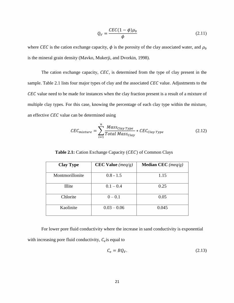
The cation exchange capacity, , is determined from the type of clay present in the

sample. Table 2.1 lists four major types of clay and the associated value. Adjustments to the

value need to be made for instances when the clay fraction present is a result of a mixture of

multiple clay types. For this case, knowing the percentage of each clay type within the mixture,

an effective value can be determined using

∑

(2.12)

Table 2.1: Cation Exchange Capacity ( of Common Clays

Clay Type CEC Value (meq/g) Median CEC (meq/g)

Montmorillonite 0.8 - 1.5 1.15

Illite 0.1 – 0.4 0.25

Chlorite 0 – 0.1 0.05

Kaolinite 0.03 – 0.06 0.045

For lower pore fluid conductivity where the increase in sand conductivity is exponential

with increasing pore fluid conductivity, is equal to

. (2.13)

22

Equation 2.12 introduces a new term which represents the equivalent conductance of the

counterions as a function of pore fluid conductivity (CW). is expressed using the empirical

formula

[ (

)] . (2.14)

The thresholds in which the sand conductivity behave exponentially and linear with

increasing pore fluid are equal to 0.06 or 6000 , respectively. A conductivity

of this value represents a pore fluid of salt water. For applications of dam integrity investigation,

the pore fluid present in the dam should have conductivity much less than 0.06 .

Therefore, when using the Waxman Smits equation to predict conductivities for the purpose of

dam evaluation, equation 2.10 should be used.

Calculations using the Waxman Smits formula to illustrate the effect of varying clay type

within a fully saturated sample are presented in Figure 2.13. The conductivity of water is plotted

on the x-axis and the total measured conductivity is plotted on the y-axis. For this plot, the

porosity and the cementation exponent are held constant at 0.36 and 2 respectively. The

median value is taken from Table 2.1 for each clay type. The value for a clayey

sample will affect the conductivity of the sample. Kaolinite and illite have similar cation

exchange capacities, therefore have similar measured conductivities. However, Montmorillonite

has a much higher cation exchange capacity compared to kaolinite and illite, therefore has a

higher measured conductivity. This helps explain when the CEC of a clayey sample increases,

the bulk conductivity of the sample will also increase.

23

Figure 2.13: Waxman Smits equation varying clay type ( = 0.36, = 2, = 1)

Calculations using the Waxman Smits equation to illustrate the effect of varying the

percentage of clay present within a fully saturated sample are shown in Figure 2.14. The

conductivity of water is plotted on the x-axis and the total measured conductivity is plotted on

the y-axis. For this plot, the porosity and the cementation exponent are held constant at 0.36

and 2 respectively. The clay type used for this analysis was montmorillonite. Each line graphed

represents a different clay percentage ranging from 10 to 100 percent. This shows that as the

percentage of clay fraction present in a sample increases, the measured conductivity also

increases.

0

0.05

0.1

0.15

0.2

0.05 0.2 0.35 0.5 0.65 0.8 0.95

CO

(m

ho/c

m)

CW (mho/cm)

Kaolinite

Montmorillonite

Illite

24

Figure 2.14: Waxman Smits equation varying clay percentage ( = 0.36, = 2, = 1)

For partially saturated shaley sand, Waxman and Smits (1968), introduces the equation

for the conductivity ( as

(

) (2.15)

The geometric factor, is a function of porosity, pore geometry, water saturation, saturation

exponent , and is independent of clay content ( . According to Archie’s second empirical

relationship, the geometric factor can be related to the saturation level below

(2.16)

Substituting equation 2.9 into equation 2.16, the geometric factor, , can be written as

(2.17)

Substituting equation 2.17 for the geometric factor, into equation 2.15 allows the total

conductivity of a partially saturated sample to be calculated using

0

0.05

0.1

0.15

0.2

0.05 0.15 0.25 0.35 0.45 0.55 0.65 0.75 0.85 0.95

CO

(m

ho

/cm

)

CW (mho/cm)

10 % Clay

40 % Clay

70 % Clay

100 % Clay

25

(

) (2.18)

2.4 Summary

Resistivity is a characteristic material property that represents the material’s ability to

oppose the flow of electrical current. The resistivity of a given soil (sand/clay) can have a wide

range values due to differing porosity ( ), saturation ( ), pore fluid resistivity ( ), and the

presence of clay content. Empirical formulas such as Archie’s Law and Waxman Smits are used

for the purpose of estimating subsurface resistivity. An understanding on how these parameters

affect resistivity measurements will aid in constructing electrical resistivity survey plans.

26

3. ELECTRICAL SURVEYS

3.1 Introduction

Different soil conditions, i.e. soil moisture and clay content, can affect the resistivity

values of soils. Electrical surveys are conducted to collect, analyze, and determine the

distribution of soil resistivity in the subsurface in the ground. These resistivity maps are used to

infer the subsurface conditions of soils and assist in the resolution of geological and engineering

problems.

Electrical surveys are conducted using injection of electric currents from point source

electrodes. The field measurements usually utilize a four electrode configuration. Two electrodes

are used for current injection and two electrodes are used for measuring the potential difference.

Several electrode arrays have been developed for field surveying. An overview of point source

electrode, electrode arrays, and a justification for the choice of the dipole/dipole array used in

this research is discussed.

3.2 Point source electrode

Consider a current injected into the soil subsurface, of uniform resistivity,, from a point

source at location A, and flows out at some infinite distance. The current will flow equally in all

directions from the point source making a hemispherical surface centered at A. Since the current

distribution is uniform on this hemispherical surface, this is a surface of constant voltage. These

27

surfaces are known as equipotential surfaces since all potentials or voltages on these surfaces are

equal.

Figure 3.1: Point source electrode (Samouelian et al., 2005)

At a given radius r from the point source, the current density, J, can be defined as

(3.1)

where I is the injected current, and is the surface area of the hemisphere. The potential

gradient from the point source at some distance r is assumed to be related to the current density

as,

(3.2)

Substituting the current density relationship into equation 3.2, and integrating the equation over

the distance r from the point source location A, the potential V can be written as

(3.3)

Solving equation 3.3 for resistivity yields,

2r2

28

(3.4)

The derivation of resistivity was gained from Griffiths and King 1965.

Measuring resistivity was originally performed using a two electrode technique. This technique

would measure the sum of the soil resistivity and the electrode/soil contact resistivity but

measurements were determined to be unpredictable. Therefore, it was decided to separate the

electrode injecting the current and the electrode measuring the potential which would reduce the

soil-electrode contact problem, therefore resulting in the creation of the four electrode method

(Pozdnyakova, 1999). Common electrical resistivity field methods now use four electrodes to

perform these surveys. In this configuration, shown in Figure 3.2, two electrodes are injecting the

current (generally labeled A and B), and the remaining two are the electrodes that measure the

potential difference (generally labeled M and N).

Using superposition, equation 3.3 is used to calculate the potential difference between electrode

M and electrode N due to a positive current at electrode A and a negative current at electrode B.

The resulting resistivity of the subsurface is given by

I

+I -I

ΔV

A M N B

AN

BM

AM BN

Figure 3.2: Four electrode setup

29

[

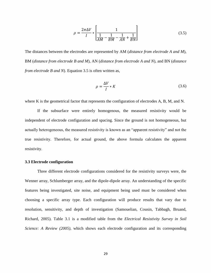
] (3.5)

The distances between the electrodes are represented by AM (distance from electrode A and M),

BM (distance from electrode B and M), AN (distance from electrode A and N), and BN (distance

from electrode B and N). Equation 3.5 is often written as,

(3.6)

where K is the geometrical factor that represents the configuration of electrodes A, B, M, and N.

If the subsurface were entirely homogenous, the measured resistivity would be

independent of electrode configuration and spacing. Since the ground is not homogeneous, but

actually heterogeneous, the measured resistivity is known as an “apparent resistivity” and not the

true resistivity. Therefore, for actual ground, the above formula calculates the apparent

resistivity.

3.3 Electrode configuration

Three different electrode configurations considered for the resistivity surveys were, the

Wenner array, Schlumberger array, and the dipole-dipole array. An understanding of the specific

features being investigated, site noise, and equipment being used must be considered when

choosing a specific array type. Each configuration will produce results that vary due to

resolution, sensitivity, and depth of investigation (Samouelian, Cousin, Tabbagh, Bruand,

Richard, 2005). Table 3.1 is a modified table from the Electrical Resistivity Survey in Soil

Science: A Review (2005), which shows each electrode configuration and its corresponding

30

strengths and weaknesses. The numbers range from low to high where the lower numbers

represent poor sensitivity and the higher numbers represent higher sensitivity.

Table 3.1: Pros and cons of common electrode configurations

Wenner

array

Schlumberger

array

Dipole-dipole

array

Sensitivity to

vertical changes 4 2 1

Sensitivity to

horizontal changes 1 2 4

Depth of

investigation 1 2 3

Horizontal data

coverage 1 2 3

Signal strength 4 3 1

Each configuration has a unique placement of the ABMN electrodes in the survey line.

Figure 3.3 illustrates the Wenner array. This array places the potential electrode pair within the

current electrode pair. Each electrode is positioned at an equal spacing of “a” from one another.

The Schlumberger electrode configuration, referred to as the Wenner-

Schlumberger array, also places the potential electrodes inside the current electrodes. This array

differs from the Wenner array because of the unequal spacing between the electrodes. The

A M N B

a a a

Figure 3.3: Wenner electrode configuration

31

distance between the electrodes A/M and B/N is equal to “n*a”, n being an integer multiple of

“a”. Figure 3.4 illustrates the Schlumberger electrode array.

The dipole-dipole configuration, pictured in Figure 3.5, differs from the previous two

array types by placing the potential electrodes outside the current electrode pair. The spacing

between current electrodes A/B and the potential electrodes M/N is of equal distance “a”. The

separation between the two sets of electrodes is equal to “n*a”, n being an integer multiple of

“a”.

3.4 Electrical Resistivity Surveys

Electrical resistivity surveys are used to investigate vertical and horizontal discontinuities

in the soil subsurface in this research. Two classical methods were commonly used to delineate

these anomalous features. The first method is known as vertical electrical sounding (locating

lateral boundaries) and the second method is known as electrical profiling (locating vertical

boundaries).

A M N B

n*a a

A M N B

n*a a n*a

Figure 3.4: Schlumberger electrode configuration

Figure 3.5: Dipole-dipole electrode configuration

32

Vertical electrical sounding (VES) is a technique in which resistivity measurements are

taken with increasing spacing between electrodes. An example of an application of this method

is to locate the depth of the water table. The deeper soil investigation is associated with the

increase in electrode spacing and provides information about the one-dimensional variation of

resistivity with depth (Samouelian et al., 2005). The Wenner electrode configuration is generally

used when VES is performed. For simplified interpretations, the ground is assumed to consist of

several horizontal layers (Samouelian et al., 2005).

Constant separation traversing, also known as electrical profiling, is another technique

used to map out the variation of resistivity of the ground. For this method, the electrode spacing

remains constant, and the electrode array is moved along in a straight line until the end of the

survey area is reached. Since the electrode spacing is constant, the CST technique will map out

lateral resistivity variations in the subsurface at a constant depth (Cardimona, n.d.). The dipole-

dipole electrode configuration is commonly used when constant separation traversing is

performed (Loke, 1999).

3.5 Building an apparent resistivity pseudosection

A combination of the VES and CST techniques can produce results illustrating a 2-

dimensional resistivity distribution of the subsurface. Separately, the VES and CST methods

obtain only 1-dimensional information of the ground and make it difficult to map both lateral and

vertical features. A common electrode setup that easily combines both vertical electrical

sounding and constant separation traversing is the dipole-dipole configuration. Referring back to

Figure 3.5, the dipole-dipole electrode configuration places the potential electrode pair outside

the current electrode pair. For this configuration, the depth of investigation is related to the

spacing between the current electrode pair, (as the “n*a” spacing increases the depth of

33

investigation increases). According to the SuperStingTM

Instruction Manual, 2005, n should not

be larger than 8 inches order to assure a strong enough signal between the current and potential

dipole. Figure 3.6 shows that the apparent resistivity is plotted at the intersection of two lines that

are drawn from the midpoint of the current electrode and potential electrode pair. The lines are

drawn at a 45o angle from the horizontal axis (Cardimona, n.d.). The actual depth of

investigation is not necessarily at the point of intersection. Also Figure 3.6 shows that as the

electrode spacing increases, the depth of investigation depth increases, but the coverage

decreases.

Figure 3.6: Dipole-dipole electrode configuration used to illustrate the location of measured

apparent resistivity (each circle represents 1 apparent resistivity measurement)

The apparent resistivity data that is collected in Figure 3.6 can be contoured to construct

an apparent resistivity pseudosection. This apparent resistivity pseudosection is an approximated

representation of the true resistivity distribution of the ground and can be used to evaluate

34

resistivity variation based on horizontal and vertical locations (Loke, 1999). Several electrode

configurations can be used to perform these surveys (i.e. Wenner, Schlumberger, dipole-dipole,

and pole-dipole). Each configuration will produce varying results due to different geometrical

factors, K, resolution, sensitivity, and depth of investigation (Samouelian et al., 2005). Figure 3.7

was plotted using EarthImager 2D Inversion software to illustrate that different electrode

configurations will produce different apparent resistivity pseudosections. The apparent resistivity

pseudosections should not be confused with true resistivity sections of the ground.

35

Figure 3.7: Apparent resistivity pseudosections for the initial survey on an embankment using

(a) Wenner array, (b) Schlumberger array, and (c) dipole-dipole array.

2 4 6 8 10 12 14 16 18 20 22 24 26

Horizontal Distance (ft)

-4

-3

-2

-1

De

pth

(ft)

13151719212325272931

a. Wenner array

2 4 6 8 10 12 14 16 18 20 22 24 26


-5

-4

-3

-2

-1

De

pth

(ft)

b. Schlumberger array

171921232527293133

2 4 6 8 10 12 14 16 18 20 22 24 26


-5

-4

-3

-2

-1

De

pth

(ft

)

111315171921232527293133353739

c. Dipole-dipole array

36

3.6 ERT inversion

ERT surveys are conducted to collect information regarding the resistivity distribution of

the subsurface. The resistivity measurements can be displayed in the form of an apparent

resistivity. However, such pseudosections are not true representations of resistivity distribution

in the subsurface. Therefore, the apparent resistivity pseudosection is converted to a true

resistivity model by an inversion process to be used for analysis and interpretation.

The imaging software, EarthImager 2D Resistivity Inversion Software, commercially

available through Advanced Geosciences Inc. is used in this thesis. The inversion process is an

iterative process that constructs a 2D image (tomogram) of the true subsurface resistivity

distribution. This process begins with a starting forward model based on the average apparent

resistivity. The forward model consists of a finite number of blocks. These blocks are updated

based upon the difference between the observed resistivity and the calculated resistivity. Both the

observed and calculated resistivities are apparent resistivity. The forward model is updated until

the user defined stop parameter is met, usually a set number of iterations or RMS error. Lastly

the forward model is inverted to produce the final inverted resistivity section (EarthImager 2D

Instruction Manual, 2007). Figure 3.8 presents an example of measured apparent resistivity

pseudosection, calculated apparent resistivity pseudosection, and the corresponding inverted

resistivity section using EarthImager 2D Resistivity Inversion Software. This figure was

constructed from a survey conducted at the research site in Stillwater, Ok.

37

Figure 3.8: Example of output from EarthImager 2D, (a) measured apparent resistivity

pseudosection, (b) calculated apparent resistivity pseudosection, and (c) inverted resistivity

section for survey conducted on embankment dam using a dipole-dipole configuration with

electrode spacing equal to 0.5 feet.

3.7 Electrode configuration selection

In this study a dam was constructed with anomalous features of known location and

dimensions. Initial electrical resistivity surveys were conducted on the dam using the three array

types described above: Wenner, Schlumberger, and dipole-dipole. These initial surveys were

processed using the EarthImager 2D Resistivity Inversion Software. The resulting tomograms for

each array type are in Figure 3.8. Each tomogram has the horizontal distance across the dam on

the x-axis, and the depth on the y-axis. The geometry, location, and size of the anomalous zones

are superimposed on the tomograms. Each tomogram is different due to the electrode

configuration. The first tomogram is the result from the Wenner array survey. This tomogram

penetrated to the shallowest depth of about 4.2ft (1.3m), and the resistivity anomalies associated

with the two zones is not pronounced. The second tomogram is the output from the survey using

a). Measured apparent resistivity pseudosection

b). Calculated apparent resistivity pseudosection

c). Inverted resistivity section

38

the Schlumberger electrode configuration. This configuration penetrated to the deepest depth of

about 5.3ft (1.6m), but again resistivity anomalies associated with the zones are not pronounced.

Also, this configuration had the longest acquisition time. The third tomogram used the dipole-

dipole electrode configuration. This electrode configuration yields the best anomalies associated

with resolution of the two compromised zones. The zones show up in the correct location, and

the values of resistivity of these zones is very similar to what was obtained from initial resistivity

measurements (during dam construction). Based on the results obtained from these three

tomograms, the dipole-dipole electrode configuration is the array of choice for our research

surveys.

39

Figure 3.9: Resistivity tomogram for the initial survey on an embankment using (a) Wenner

array, (b) Schlumberger array, and (c) dipole-dipole array

0 2 4 6 8 10 12 14 16 18 20 22 24 26 28


-4

-3

-2

-1

0D

ep

th (

ft)

35916284987153

a. Wenner Array

0 2 4 6 8 10 12 14 16 18 20 22 24 26 28


-5

-4

-3

-2

-1

0

De

pth

(ft

)

b. Schlumberger Array

1216202633435571

0 2 4 6 8 10 12 14 16 18 20 22 24 26 28


-5

-4

-3

-2

-1

0

De

pth

(ft

)

8121828426498150

c. Dipole-Dipole Array

40

3.8 Summary

Electrical resistivity surveys inject current into the ground through electrodes that are

arranged in a specified geometry. The measured apparent resistivity is related to the injected

current, measured voltage, and geometrical position of the electrodes and should be not be

confused with the true resistivity of the subsurface. As such pseudosections are not true

representations of the resistivity distribution in the subsurface. The apparent resistivity

pseudosection must be converted to a true resistivity section by an inversion process, which is

used for analysis and interpretation.

Each electrode configuration and electrical survey has strengths and weaknesses. An

understanding of the subsurface and the type/size of the anomaly being detected must be

considered before selecting an appropriate electrode configuration. For our investigation of

localized zones associated with seepage and piping through an embankment dam the dipole-

dipole array appear to perform best.

41

4. FORWARD MODELING

4.1 Introduction

The electrical resistivity depends on the amount of moisture and clay content in soils and

has been used to help investigate earthen embankment dams. The electrical signature of a

compromised zone associated with seepage and piping will not only depend on the electrical

resistivity of the material within the zone but also on the size and location of the zone.

In order to determine the electrical signature of compromised zones within an

embankment, forward modeling is performed using the modeling option in the EarthImager 2D

software. Synthetic models are created based upon assumptions of the subsurface resistivity

distribution and electrode configuration (EarthImager 2D Instruction Manual, 2007). The

objective of the forward models is to gain an understanding of how the size, contrast, and depth

of anomalous zones along with random noise will affect the detection and resolution of these

zones. Forward modeling helps to optimize survey plans which result in a reduction of survey

time in the field. An overview of the forward modeling features in EarthImager 2D is presented.

This modeling software is used to investigate the effects of zone size and resistivity contrast on

the electrical signatures. The resolution of the ERT method on zone depth and degree of random

noise is also evaluated.

4.2 Forward modeling using EarthImager 2D

Also known as survey planning, forward modeling using EarthImager 2D software is a

two-step process. The first step is to create a synthetic model based upon assumed resistivity

distributions of the subsurface and the electrode configuration. This step is called forward

42

simulation which calculates a synthetic data set (apparent resistivity pseudosection) based upon

the constructed synthetic model. The second step is to invert the synthetic data set. The goal of

the inversion procedure is to recreate the resistivity distribution assumed in the synthetic model.

The inverted model is compared to the original synthetic model in order to evaluate the

resolution and detection capability. This process will provide an intuition on the applicability of

the electrical resistivity method for solving a particular problem (EarthImager 2D Instruction

Manual, 2007).

4.3 Zone detection

This section illustrates how the size of the zone and the contrast between the zone and the

background resistivity affect detection. The synthetic model created to test the sensitivity to zone

size uses 56 electrodes arranged in a dipole-dipole array. Dimensions of the model are scaled

with respect to the electrode spacing. The total spread length, , is a function of the electrode

spacing, , such that

(4.1)

The depth of penetration, , is a function of the total spread length, and can be

estimated by

(4.2)

The background resistivity in the starting model is 200 ohm*m and the zone resistivity is

100 ohm*m, a contrast of 2 to 1. The initial model sets the dimensions of the zone to 1 ES x 1

ES, a function of the electrode spacing. A random noise of 1 % is used for the analysis. Figure

4.1 illustrates the initial synthetic model used to test the dependence on the zone size. The zone

43

size for each model will increase by 1 ES x 1 ES until the zone can be easily detected in the

inverted tomogram. The size of the zone is increased uniformly about its centroid, which is

located at a depth of 4.5 electrode spacing.

Figure 4.1: Synthetic model created to study the dependence on zone size. The zone resistivity is

½ the background resistivity and is placed at a depth of 4.5 electrode spacing.

Using the model created, a forward simulation produced a synthetic data set. This

synthetic data set is then processed using algorithms in EarthImager 2D. Figure 4.2 to 4.4 are the

inverted results for different zone sizes. The horizontal distance along the survey spread is

plotted on the x-axis, the depth in the subsurface is plotted on the y-axis. The resistivity (ohm*m)

is represented as intensity values.

Figure 4.2: Tomogram for zone size equal to 1 ES x 1 ES

0 5 10 15 20 25 30 35 40 45 50 55

Horizontal Distance

-10

-5

0

De

pth

180185190195200205210215220225230

44

Figure 4.3: Resistivity tomogram for zone size equal to 2 ES x 2 ES

Figure 4.4: Resistivity tomogram for zone size equal to 3 ES x 3 ES

The three inverted tomograms illustrate that a zone with its centroid located at a depth of

4.5 ES in the subsurface with dimensions of 3 ES x 3 ES can be easily detected using electrical

resistivity tomography. A zone with dimensions of 2 ES x 2 ES is detected within the tomogram,

but its shape is somewhat distorted.

The contrast between the zone resistivity and the background resistivity can influence

zone detection. Cases where the resistivity of the zone is lower than the background and when

the zone resistivity is higher than the background resistivity are compared. Figure 4.5 is the

synthetic model used to test the sensitivity to the resistivity contrast. The size of the zone is set to

3 ES x 3 ES and the depth is set to 3 ES. The electrode configuration chosen for this analysis was

the dipole-dipole array and the level of random noise was set to 1%.

0 5 10 15 20 25 30 35 40 45 50 55

Horizontal Distance

-10

-5

0

De

pth

169177185193201209217225233

0 5 10 15 20 25 30 35 40 45 50 55

Horizontal Distance

-10

-5

0

De

pth

146158170182194206218

45

Figure 4.5: Synthetic model created for analysis of sensitivity to resistivity contrast

variation. Zone dimensions are 3 ES x 3 ES. Zone is placed at a depth of 3

electrode spacing.

Figure 4.6 to 4.8 are the results for which the zone has a lower resistivity than the

background resistivity. For this scenario, the background resistivity remains constant at 200

ohm*m and the resistivity of the zone is allowed to vary. As the contrast between the

background and zone increase, detection of the zone in the data set is possible. Zones with

contrasts smaller than 1.33:1 are not detected.

Figure 4.6: Resistivity tomogram with contrast of 1.14:1 (200 ohm*m to 175 ohm*m)

0 5 10 15 20 25 30 35 40 45 50 55

Horizontal Distance

-10

-5

0

De

pth

169177185193201209217225

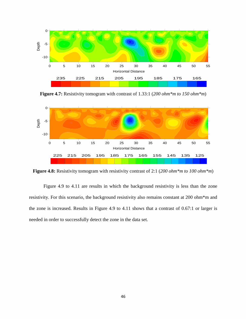
46

Figure 4.7: Resistivity tomogram with contrast of 1.33:1 (200 ohm*m to 150 ohm*m)

Figure 4.8: Resistivity tomogram with resistivity contrast of 2:1 (200 ohm*m to 100 ohm*m)

Figure 4.9 to 4.11 are results in which the background resistivity is less than the zone

resistivity. For this scenario, the background resistivity also remains constant at 200 ohm*m and

the zone is increased. Results in Figure 4.9 to 4.11 shows that a contrast of 0.67:1 or larger is

needed in order to successfully detect the zone in the data set.

0 5 10 15 20 25 30 35 40 45 50 55

Horizontal Distance

-10

-5

0

De

pth

165175185195205215225235

0 5 10 15 20 25 30 35 40 45 50 55

Horizontal Distance

-10

-5

0

De

pth

125135145155165175185195205215225

47

Figure 4.9: Resistivity tomogram with resistivity contrast of 0.89:1 (200 ohm*m to 225 ohm *m)

Figure 4.10: Resistivity tomogram with resistivity contrast of 0.8:1 (200 ohm*m to 250 ohm *m)

Figure 4.11: Resistivity tomogram with resistivity contrast of 0.67:1 (200 ohm*m to 300

ohm*m)

0 5 10 15 20 25 30 35 40 45 50 55

Horizontal Distance

-10

-5

0

De

pth

175185195205215225

0 5 10 15 20 25 30 35 40 45 50 55

Horizontal Distance

-10

-5

0

De

pth

180185190195200205210215220225230235

0 5 10 15 20 25 30 35 40 45 50 55

Horizontal Distance

-10

-5

0

De

pth

168180192204216228240252264

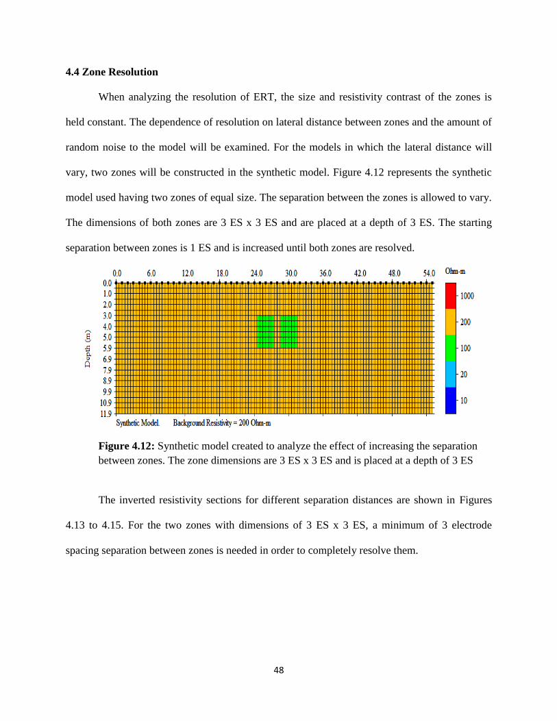
48

4.4 Zone Resolution

When analyzing the resolution of ERT, the size and resistivity contrast of the zones is

held constant. The dependence of resolution on lateral distance between zones and the amount of

random noise to the model will be examined. For the models in which the lateral distance will

vary, two zones will be constructed in the synthetic model. Figure 4.12 represents the synthetic

model used having two zones of equal size. The separation between the zones is allowed to vary.

The dimensions of both zones are 3 ES x 3 ES and are placed at a depth of 3 ES. The starting

separation between zones is 1 ES and is increased until both zones are resolved.

Figure 4.12: Synthetic model created to analyze the effect of increasing the separation

between zones. The zone dimensions are 3 ES x 3 ES and is placed at a depth of 3 ES

The inverted resistivity sections for different separation distances are shown in Figures

4.13 to 4.15. For the two zones with dimensions of 3 ES x 3 ES, a minimum of 3 electrode

spacing separation between zones is needed in order to completely resolve them.

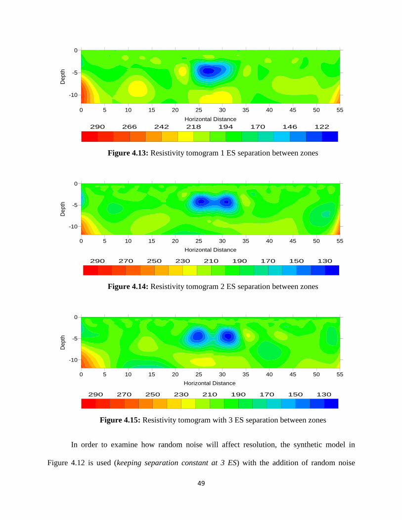
49

Figure 4.13: Resistivity tomogram 1 ES separation between zones

Figure 4.14: Resistivity tomogram 2 ES separation between zones

Figure 4.15: Resistivity tomogram with 3 ES separation between zones

In order to examine how random noise will affect resolution, the synthetic model in

Figure 4.12 is used (keeping separation constant at 3 ES) with the addition of random noise

0 5 10 15 20 25 30 35 40 45 50 55

Horizontal Distance

-10

-5

0

Dep

th

122146170194218242266290

0 5 10 15 20 25 30 35 40 45 50 55

Horizontal Distance

-10

-5

0

De

pth

130150170190210230250270290

0 5 10 15 20 25 30 35 40 45 50 55

Horizontal Distance

-10

-5

0

De

pth

130150170190210230250270290

50

levels of 1%, 3%, and 6%. Increasing the noise in the model causes an increase in the RMS error

for each inversion. The inverted data is shown in Figures 4.16 to 4.18. It is possible to resolve the

zones in with random noise levels of 1% and 3%. However, with a random noise level of 6%, the

zone can no longer be distinguished. In this research, a level of 6% noise was never reached.

Figure 4.16: Resistivity tomogram with a random noise level of 1%

Figure 4.17: Resistivity tomogram with a random noise level of 3%

0 5 10 15 20 25 30 35 40 45 50 55

Horizontal Distance

-10

-5

0

Dep

th

130150170190210230250270

0 5 10 15 20 25 30 35 40 45 50 55

Horizaontal Distance

-10

-5

0

De

pth

130150170190210230250270290310

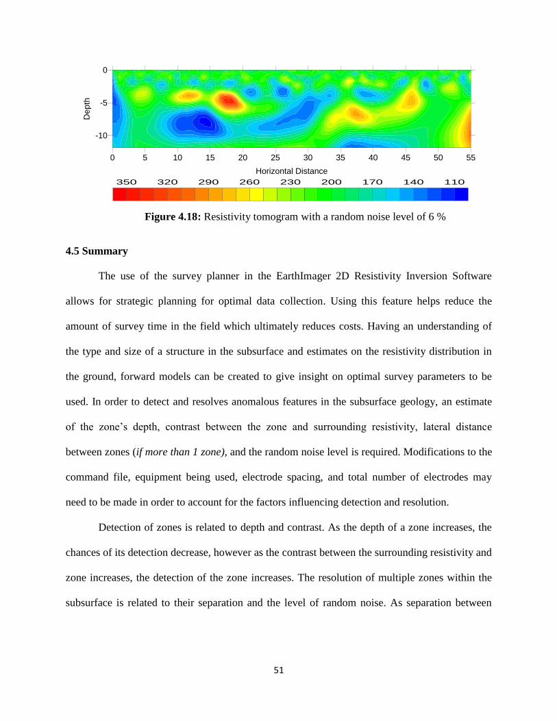
51

Figure 4.18: Resistivity tomogram with a random noise level of 6 %

4.5 Summary

The use of the survey planner in the EarthImager 2D Resistivity Inversion Software

allows for strategic planning for optimal data collection. Using this feature helps reduce the

amount of survey time in the field which ultimately reduces costs. Having an understanding of

the type and size of a structure in the subsurface and estimates on the resistivity distribution in

the ground, forward models can be created to give insight on optimal survey parameters to be

used. In order to detect and resolves anomalous features in the subsurface geology, an estimate

of the zone’s depth, contrast between the zone and surrounding resistivity, lateral distance

between zones (if more than 1 zone), and the random noise level is required. Modifications to the

command file, equipment being used, electrode spacing, and total number of electrodes may

need to be made in order to account for the factors influencing detection and resolution.

Detection of zones is related to depth and contrast. As the depth of a zone increases, the

chances of its detection decrease, however as the contrast between the surrounding resistivity and

zone increases, the detection of the zone increases. The resolution of multiple zones within the

subsurface is related to their separation and the level of random noise. As separation between

0 5 10 15 20 25 30 35 40 45 50 55

Horizontal Distance

-10

-5

0

De

pth

110140170200230260290320350

52

two zones increases, the zones become easier to resolve in the data set, but as the random noise

level increases, resolving the zones in the data set becomes more of a challenge.

53

5. FIELD MEASUREMENTS AND DISCUSSION OF RESULTS

5.1 Introduction

Electrical resistivity methods have the potential to provide information regarding internal

problems (seepage/ internal erosion) of earthen embankment dams. In this chapter, information

from electrical resistivity tomography surveys conducted on an experimental dam is discussed.

An overview of the embankment dam including: geometrical dimensions, soil analysis,

and in-situ sensors is presented followed by a description of the electrical resistivity equipment

and acquisition parameters. A schedule of the field trips and results from the electrical resistivity

surveys performed over the course of this research are presented.

5.2 Description of embankment dam

A quarter-scale experimental embankment dam was constructed at the USDA-ARS

Hydraulic Engineering Research Unit (HERU) located in Stillwater, Oklahoma. The HERU

facility provided the equipment, materials, and personnel in order to construct the dam at its

research laboratory. The dam was constructed over the period of a month.

The earthen embankment was completed near the end of September 2010, and electrical

resistivity surveys began approximately three weeks after. The embankment structure was built

to a height of 4 ft (1.25 m), a length of 28 ft (8.5 m) across the top, a crest width of 6.5 ft (≈ 2.0

m), 3 to 1 side slopes, and 1 to 1 abutment slopes. Figure 5.1 shows a cross section of the

embankment.

54

Figure 5.1: Schematic of embankment geometry

The body of the dam was a clayey loam compacted at a moisture content of 14%

(optimum moisture content). The HERU personnel designed and compacted each lift of material.

After compaction of each layer, a sample of soil was obtained and the corresponding moisture

content and dry bulk density was determined. A total of 11 lifts were needed to meet the dam’s

specifications. Table 5.1 contains soil data from each constructed lift.

The soil used to construct the dam has been used previously on projects at the HERU

research facilities. Laboratory tests performed on the clay loam obtained the maximum dry

density and the optimum water content at standard compaction (Hanson and Hunt, 2007). The

clayey loam laboratory test results are comparable to those presented in Table 5.1.

55

Table 5.1: Lift information for experimental embankment dam

Layer

#

Date

Placed

Avg. Moisture

(%)

Avg. Dry Density

(g/cc) Porosity Saturation

1 8/20/2010 15.4 1.78 0.33 0.84

2 8/23/2010 12.5 1.76 0.33 0.66

3 8/26/2010 12.7 1.81 0.31 0.73

4 8/27/2010 13.4 1.78 0.33 0.73

5 8/30/2010 13.1 1.80 0.32 0.74

6 9/1/2010 14.5 1.77 0.33 0.78

Sand 9/2/2010 9.3 1.70 0.36 0.44

Dry

Clay 9/7/2010 9.3 1.65 0.38 0.41

7 9/16/2010 13.7 1.78 0.33 0.75

8 9/20/2010 13.0 1.78 0.33 0.71

9 9/21/2010 13.2 1.76 0.33 0.70

10 9/22/2010 15.4 1.78 0.33 0.84

11 9/22/2010 13.8 1.70 0.36 0.66

The dam was constructed with two compromised zones that would be susceptible to

seepage and piping. The first zone was a dryer compacted clay zone, and the second was a sandy

56

zone. The dryer clay layer was compacted with the same energy as the dam body but at a

moisture content of 10%, which is four percent lower than optimum moisture. This zone is meant

to represent a possible construction mishap in the field during the construction of an

embankment dam. This zone will have a higher porosity than the dam body, therefore causing an

initial higher resistivity. The sandy layer was a zone composed of a more porous material with a

higher permeability. This zone is meant to represents a natural geologic feature such as a sand

lens that might be located under a real dam. However for construction simplicity, this zone was

placed inside the dam. These two anomalous features have geometrical dimensions of 6 ft x 1 ft

and run from the upstream side of the dam through to the downstream side. On the upstream

side, these zones were protected by 3 feet of compacted clay material. Figure 5.2 shows a plan

view of the dam, illustrating the size and placement of these zones.

The dam was to be constructed at optimum moisture content (14%) because this causes

the dam to be stiffer and have a higher permeability, which will help induce seepage. A second

dam was built at the HERU facilities in Stillwater, OK with moisture content of 3% above

optimum. This causes the embankment to have a lower stiffness and a lower permeability. The

second dam’s reservoir remained loaded for a period of six months and no signs of seepage were

visible. Additional data were collected on this dam but is not presented in this thesis.

57

Sieve analysis of the dam material is listed in Table 5.2. The clay loam was used to

construct both the dam body and the dryer compacted clay zone, and the sandy loam was used

for the compromised sand zone. The sieve classifications for sand, silt, and clay are 0.84 to 0.05

mm for sand, 0.05 to 0.002 mm for silt, and material smaller than 0.002 mm sieve is classified as

clay. According to the sieve results, the clay loam consists of 30% sand, 44% silt, and 26% clay.

For the sandy loam, the material was divided into 84% sand, 9% silt, and 7% clay. For the clay

loam, the liquid limit (LL) and plasticity index (PI) was determined to be 29 and 17,

respectively.

CL

20`

6` 6`

3`

28`

10`

Dry

Clay

Sand

Figure 5.2: Plan view of embankment dam

58

Table 5.2: Sieve analysis of embankment soils

Clay Loam Sandy Loam

Sieve Size (mm) Percent Passing By Weight Percent Passing By Weight

0.84 100 100

0.42 100 95

0.25 100 77

0.105 100 40

0.074 79 26

0.05 70 16

0.02 49 8

0.005 35 8

0.002 26 7

LL 29

PI 17

Specific Gravity 2.69 2.65

X-ray diffraction tests were performed on the clay loam sample to obtain a classification

based on the mineralogy and not the particle size. This sample consists of 80% sand, 15% clay,

and 5% feldspars (sand). The X-ray diffraction indicates that of the 15% clay, among this 15%

clay, 7% was Kaolinite, 5% was Smectite (Montmorillonite), and 3% was Mica (Illite).

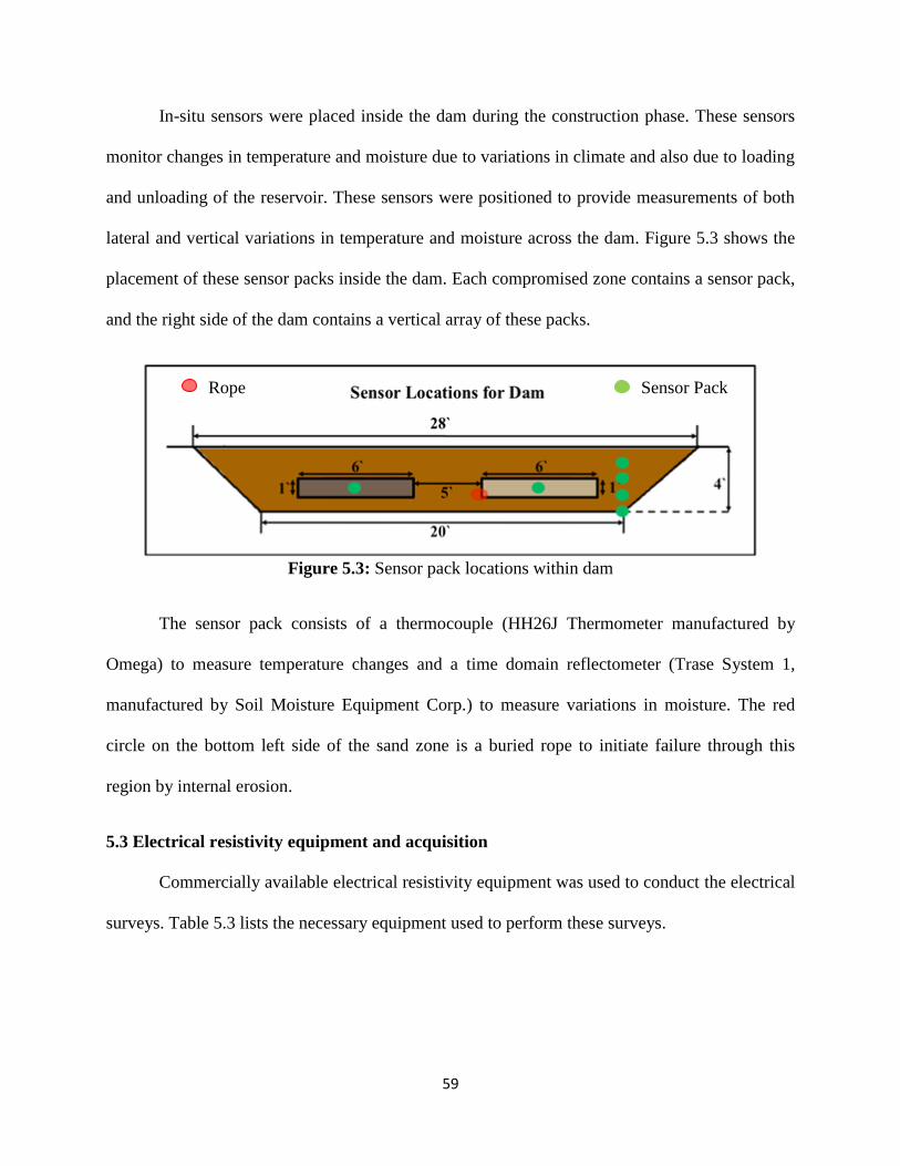
59

In-situ sensors were placed inside the dam during the construction phase. These sensors

monitor changes in temperature and moisture due to variations in climate and also due to loading

and unloading of the reservoir. These sensors were positioned to provide measurements of both

lateral and vertical variations in temperature and moisture across the dam. Figure 5.3 shows the

placement of these sensor packs inside the dam. Each compromised zone contains a sensor pack,

and the right side of the dam contains a vertical array of these packs.

Figure 5.3: Sensor pack locations within dam

The sensor pack consists of a thermocouple (HH26J Thermometer manufactured by

Omega) to measure temperature changes and a time domain reflectometer (Trase System 1,

manufactured by Soil Moisture Equipment Corp.) to measure variations in moisture. The red

circle on the bottom left side of the sand zone is a buried rope to initiate failure through this

region by internal erosion.

5.3 Electrical resistivity equipment and acquisition

Commercially available electrical resistivity equipment was used to conduct the electrical

surveys. Table 5.3 lists the necessary equipment used to perform these surveys.

Sensor Pack Rope

60

Table 5.3: List of equipment used for ERT surveys

Major Equipment Supplementary Equipment

SuperStingTM

R8/IP resistivity meter,

SuperStingTM

switch box 56 electrode

system, passive cables with 14 electrode

switches per cable, stainless steel

electrodes-stake with springs,

connection/communication cables,

SuperStingTM

administrator software, and

EarthImager 2D inversion software

12 volt battery, tape measure, hammer,

flags, and field laptop

61

A SuperStingTM

R8/IP resistivity meter is shown in Figure 5.4. Powered by a standard 12

volt car battery, the resistivity meter is responsible for supplying current into the ground. The

meter used in this research is built with 8 receivers. For each current injection, the potential

difference between nine electrodes can be measured at the same time, resulting in shorter survey

times (SuperStingTM

Instruction Manual, 2005).

Figure 5.4: SuperStingTM

R8 resistivity meter

The resistivity meter does not have a built-in switch system; therefore, an external switch

box is required. A switch box is pictured in Figure 5.5. This system is referred to as a central

switching system. Each electrode switch has a specific lead in the cable that is attached directly

to the switch box. The switch box is connected directly to the resistivity meter. The switch box

can directly assign which electrode will be used as the current electrode (A or B) or the potential

electrode (M or N). The assignment depends directly on how the command file is constructed.

The switch box has the capability of switching up to 56 electrodes (SuperStingTM

Instruction

Manual, 2005).

62

Figure 5.5: Switch box

Electrode stakes and electrode switches are pictured in Figure 5.6. The electrode stakes

are stainless steel rods and are attached to the electrode switch by using a spring. Each coil of

cable contains 14 electrode switches (1 coil shown below). For a 56 electrode system, 4 spools of

electrode switch cable are needed. Each electrode switch has a lead in the cable that is connected

to the switch box. The switches are numbered uniquely and have the capability of being

reprogrammed if needed (SuperStingTM

Instruction Manual, 2005).

Figure 5.6: Electrode stakes and switches

For the electrical resistivity surveys in this research, 56 electrode stakes are arranged on

the dam crest in a 2D linear array. An electrode spacing of 0.6 feet (0.18 m) is used. Figure 5.7 is

a photograph of the field setup. This figure shows that the stakes are connected to the electrodes

63

switches by a stainless steel spring which are then connected to the switch box. The resistivity

meter and the switch box are joined by a 2 meter jumper cable. Two 12 volt batteries power the

system. The placement of the meter and switch box is at the center of the electrode spread

(between electrode 28 and 29).

Figure 5.7: Field setup of ERT equipment

The electrode configuration chosen for these surveys was the dipole-dipole array. A

command file was created using the AGI administrator software and was uploaded to the

resistivity meter. Before running a survey, important parameters regarding the setup of the data

files are chosen using the display screen on the resistivity meter. These parameters are listed in

Table 5.4.

64

Table 5.4: Resistivity meter parameters

Parameter Parameter settings

Scaling Factor 0.18 meters

Number of Cycles 3 cycles

Maximum Error 1 %

Maximum Current 2000 mA

When creating the command file, the software assumes the electrode spacing is 1 meter.

Therefore, when setting up the survey on the resistivity meter, a scaling factor needs to be set in

order to increase or decrease the electrode spacing. The number of cycles, also referred to as

stacking (SuperStingTM

Instruction Manual, 2005) has a minimum setting 2 cycles. During the

measurement the meter calculates the average and standard deviation of successive

measurements. The maximum error is a threshold value for the standard deviation (mentioned

above). If the standard deviation is lower than the threshold value set by the user, the stacking

will be interrupted and the meter will move on to the next measurement (SuperStingTM

Instruction Manual, 2005). The factory setting for the maximum error is 2 %. The maximum

current for each measurement is defaulted at 1250 mA.

A quality control measure is performed before a survey is conducted known as a contact

resistance test. This test evaluates the contact between the electrode stakes and the ground along

the profile. Poor contact between the electrodes and the ground can produce noisy data. For

instances in which poor contact (high resistance values are displayed on the meter) occurs, water

is poured in the area surrounding the electrode to enhance electrical contact.

65

5.4 Schedule of surveys

Five trips were made to the HERU facilities to conduct surveys on the experimental

embankment dam. Weather permitting, each trip usually lasted 5 days. The first of the series of

trips was made after the completion of the dam in the middle of October 2010. The purpose of

this trip was to obtain an initial set of resistivity data in order to construct a baseline tomogram

for future measurements. The remaining trips consisted of surveying on the dam during cyclic

loading of the reservoir. The first day of each trip was used to setup the equipment and obtain

preliminary measurements on the dam with an empty reservoir. Then in the afternoon, the

reservoir was usually loaded. Surveys were continually conducted on the dam until seepage was

visible on the downstream side of the dam. The seepage process generally evolved over a period

of three to four days. The dates of each survey along with the corresponding reservoir condition,

electrode configuration, and electrode spacing is presented in Appendix 1. Wenner, inverted

Schlumberger, and dipole-dipole configurations were all used on the initial trip in order to

determine which array would produce the best resolution for the detection of the compromised

zones. As discussed in Chapter 3, the dipole-dipole configuration was chosen for the remaining

surveys. The Schlumberger and inverted Schlumberger arrays were used intermittently, but the

zones could not be resolved in the resulting tomograms with these configurations.

5.5 Discussion of results

Measurement take from the in-situ sensors installed in the dam during construction as

well as the numerous ERT survey results were analyzed and interpretations were made.

66

5.5.1 Results from in situ sensors

i). TDR in-situ sensors

Personnel at the HERU facility recorded weekly readings from the in-situ sensors

embedded in the dam during the construction phase (Figure 5.3). During survey trips to

Stillwater, OK, multiple readings were taken daily. These readings are displayed as a cluster of

points in each plot. These sensors provide moisture and temperature variations inside the dam

that may be associated with seepage from rainfall and seepage from the loaded reservoir. Figure

5.8 illustrates TDR data from four sensors placed at a depth of 2 feet and provides information

about the lateral variations in moisture inside the dam. Figure 5.9 plots moisture readings from

TDR sensors arranged in a vertical array on the right side of the dam. The date of the

measurement is plotted on the x-axis, the moisture content reading in percent is plotted on the

primary y-axis, and the measured precipitation in inches is plotted as a secondary y-axis. The

precipitation readings were collected from the Oklahoma Mesonet website, devoted to

monitoring environmental weather events in the State of Oklahoma.

The moisture readings from the TDR sensors are in terms of volumetric water content.

The measured values from the TDR sensor should range from 0 to porosity. In other words, for a

soil sample that is fully dried, the TDR sensor should read 0, and for a soil sample that is fully

saturated, the TDR sensor should read a value equal to its porosity.

Figure 5.8 represents the lateral variations of moisture content in the dam. When the dam

was constructed, the dam body material was compacted at higher moisture content than the dry

clay zone and the sand zone. This is supported by the initial TDR measurements. The moisture

measurements remained rather constant until the middle of November 2010. According to the

Mesonet readings, a heavy rainfall occurred resulting in large amounts of infiltration of

67

precipitation into the dam. The TDR sensors responded to this rainfall and recorded an increase

in moisture. The dry clay originally had lower moisture content than the dam body, but was

constructed with a higher porosity. The infiltration of precipitation filled this larger porosity

resulting in the larger measured volumetric water content as shown in Figure 5.8. The TDR

measurements remained constant during subsequent rainfall in the month of March 2011. This

may be due to the soil acquiring its natural holding limits of water (field capacity) where

additional rainfall would not further increase the saturation levels. Starting in the month of April

2011, the TDR sensors show a decrease in moisture content in the sand zone and dry clay zone.

The TDR sensors did not respond to the large amount of rainfall that occurred during the month

of May 2011. The abrupt increase observed at the end of May 2011 is caused by seepage from

the loaded reservoir during one of the trips. The drastic decrease in moisture content measured

from June 2011 to August 2011 by all three TDR sensors are associated with extreme

temperatures and very limited amounts of rainfall (drought). The abrupt increase at the end of the

graph is again related to seepage from a loaded reservoir.

68

Figure 5.8: Moisture content plot for embankment (lateral variation)

The TDR measurements that provide a measure of the vertical variation of moisture

content in the dam body are presented in Figure 5.9. The TDR labeled 0 ft is located at the

basement of the dam, the TDR labeled 1ft is located 1 foot above the basement of the dam, the

TDR labeled 2 ft is positioned 2 feet above the basement of the dam, and the TDR labeled 3 ft is

located three feet above the dam basement (1 foot below the dam crest). A goal when

constructing the embankment was to compact the dam body material at a consistent moisture

content. The TDR sensors show that the clayey material compacted from the basement (0 ft) up

to an elevation of 3 feet (2 ft) does in fact have uniform moisture contents, but the top 1 ft of clay

was compacted at much lower moisture content. This could be associated with the material being

exposed to the air for a longer period of time before being compacted in the dam causing it to dry

out.

0

0.2

0.4

0.6

0.8

1

1.2

1.4

1.6

1.8

0

5

10

15

20

25

30

35

40

Pre

cip

iati

on

(in

)

Mois

ture

Con

ten

t (%

)

Date of Measurement

Rainfall (in)

Sand

Dry Clay

2 ft

69

When the rainfall in November, 2010 infiltrated the dam, all TDR sensors responded and

measured an increase in moisture content. After this rain, the sensors located at the basement of

the dam had the highest moisture content and the sensor located near the crest of the dam had the

lowest moisture content. The only fluctuations in measurements were during cyclic loading

events in which abrupt increases are noticeable in the data caused by seepage from the reservoir.

The constant behavior of the dam material (except for reservoir loading) suggests that this

material has reached its natural holding capacity of water. In such a case the increased rainfall

during the spring months would have no additional effect on the moisture content from the TDR

readings. From the months of June 2011 to August 2011, the TDR sensors measured a large

decrease in moisture content associated with extreme temperatures and drought like conditions.

The last trip made during August, the reservoir was loaded and the abrupt increases in moisture

content are caused by seepage water pouring through the cracks along the dam.

Figure 5.9: Moisture content plot for embankment (vertical variation)

0

0.2

0.4

0.6

0.8

1

1.2

1.4

1.6

1.8

0

5

10

15

20

25

30

35

40

Rain

fall

(in

)

Mois

ture

Con

ten

t (%

)

Date of Measurement

Rainfall (in)

0 ft

1 ft

2 ft

3 ft

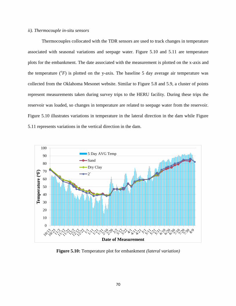
70

ii). Thermocouple in-situ sensors

Thermocouples collocated with the TDR sensors are used to track changes in temperature

associated with seasonal variations and seepage water. Figure 5.10 and 5.11 are temperature

plots for the embankment. The date associated with the measurement is plotted on the x-axis and

the temperature (oF) is plotted on the y-axis. The baseline 5 day average air temperature was

collected from the Oklahoma Mesonet website. Similar to Figure 5.8 and 5.9, a cluster of points

represent measurements taken during survey trips to the HERU facility. During these trips the

reservoir was loaded, so changes in temperature are related to seepage water from the reservoir.

Figure 5.10 illustrates variations in temperature in the lateral direction in the dam while Figure

5.11 represents variations in the vertical direction in the dam.

Figure 5.10: Temperature plot for embankment (lateral variation)

0

10

20

30

40

50

60

70

80

90

100

Tem

per

atu

re (

oF

)

Date of Measurement

5 Day AVG Temp

Sand

Dry Clay

2`

71

Figure 5.11: Temperature plot for embankment (vertical variation)

The measurements in Figure 5.10 show that the temperatures across the dam are very

similar to one another. The temperature of the dam tracks the seasonal temperature changes in

Oklahoma. According to Figure 5.11, the thermocouple temperatures measured in the colder

months at deeper depths were higher at depth than those located closer the surface. In the hotter

months, such as August, the thermocouple temperature deeper in the dam had lower

temperatures than the ones located closer to the surface.

5.5.2 ERT tomogram results related to environmental changes

The ERT tomograms for the first survey conducted from each trip can be representative

to changes in environmental conditions (seasonal variations) experienced between trips. Each

tomogram is a slice through the embankment and is oriented to look upstream. The x-axis is the

distance across the dam crest and the y-axis is depth in the dam. Both axes have units of feet.

The intensity values for high resistivity are assigned colors of red and orange and low resistivity

0

10

20

30

40

50

60

70

80

90

100

Tem

per

atu

re (

oF

)

Date of Measurement

5 Day AVG Temp

0 ft

1 ft

2 ft

3 ft

72

values have colors of blue. Lower resistivity values indicate areas of higher moisture while dryer

areas are indicated by higher resistivity. A schematic of the dam is drawn on top of each

tomogram to help illustrate the size and placement of the compromised zones. As described in

Figure 5.1, the dryer compacted clay zone is located on the left side of the dam and the sand zone

is located on the right.

The tomogram for the first ERT survey conducted in October 2010 is presented in Figure

5.12. This survey was conducted using a dipole-dipole configuration with an electrode spacing

equal to 0.15m. The results show that both the sand zone and dry clay zone are detected in the

tomogram and appear in their appropriate locations. Higher levels of moisture are detected

around both the left and right abutments and show up as low resistivity bull-eyes. Also a high

resistivity band is evident at a depth of 1 foot in the dam. This might be related to a variation in

moisture of the clay material used during dam construction.

i). October 2010 to November 2010

The tomogram for the first ERT survey (empty reservoir) conducted in late November

2010 is presented in Figure 5.13. Slight differences between the setup/acquisition for the survey

conducted in October and November include a change in electrode spacing and the addition of

Figure 5.12: Electrical resistivity tomogram for survey conducted October 13, 2011 at

15:45. Reservoir is empty.

73

sod to the dam. The electrode spacing used for the survey conducted in October was 0.15m

whereas the electrode spacing used in the November survey was 0.28m. The increase in

electrode spacing between trips results in a reduction in the resolution for the tomogram shown

in Figure 5.13. The absence of the lateral high resistivity zone at a shallow depth across the

November tomogram may be due to a reduced surface drying associated with the addition of sod.

An overall reduction in resistivity of the dam is observed from October to November.

This is attributed to the infiltration of rainwater into the dam over this period of time. The

Mesonet readings indicate a substantial amount of precipitation a few weeks before the survey

was conducted in November. The precipitation caused an increase in moisture in the dam and is

supported by measurements taken from the in-situ TDR sensors. The decrease in resistivity of

the sand zone between October and November is also associated with an increase in moisture of

the sand zone. This is supported by the TDR sensor plots in Figure 5.9. Furthermore, the contrast

between dry compacted clay zone and the dam body observed in the October survey is no longer

present in the November survey. This is caused by a decrease in the zone’s resistivity due to a

substantial increase in moisture as recorded by the TDR sensors.

Figure 5.13: Electrical resistivity tomogram for survey conducted November 29, 2011

at 11:30. Reservoir is empty.

0 2 4 6 8 10 12 14 16 18 20 22 24 26 28

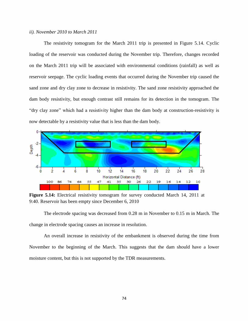
74

ii). November 2010 to March 2011

The resistivity tomogram for the March 2011 trip is presented in Figure 5.14. Cyclic

loading of the reservoir was conducted during the November trip. Therefore, changes recorded

on the March 2011 trip will be associated with environmental conditions (rainfall) as well as

reservoir seepage. The cyclic loading events that occurred during the November trip caused the

sand zone and dry clay zone to decrease in resistivity. The sand zone resistivity approached the

dam body resistivity, but enough contrast still remains for its detection in the tomogram. The

“dry clay zone” which had a resistivity higher than the dam body at construction-resistivity is

now detectable by a resistivity value that is less than the dam body.

The electrode spacing was decreased from 0.28 m in November to 0.15 m in March. The

change in electrode spacing causes an increase in resolution.

An overall increase in resistivity of the embankment is observed during the time from

November to the beginning of the March. This suggests that the dam should have a lower

moisture content, but this is not supported by the TDR measurements.

Figure 5.14: Electrical resistivity tomogram for survey conducted March 14, 2011 at

9:40. Reservoir has been empty since December 6, 2010

75

iii). March 2011 to May 2011

The tomogram for the survey conducted in May 2011 is shown in Figure 5.15. The

setup/acquisition is the same for both trips; therefore, the changes in the tomograms should be

strictly a function of environmental changes and the previous loading of the reservoir. The

resistivity of the dam body has decreased during this time period. This would suggest a decrease

in moisture content of the dam body and can be confirmed by the decrease in the moisture

readings measured by the TDR sensors after the March trip. The Mesonet shows a substantial

amount of precipitation just before the May trip; however, the TDR sensors do not respond to

this rainfall. This may be due to increased temperatures during this time which helped the dam

dry out.

The contrast between the sand zone and the dam body increased in the May tomogram. This

increase in contrast is related to an increase in resistivity of the sand zone which is supported by

the decrease in moisture recorded by the TDR sensors in Figure 5.8. Similar to the sand zone, the

resistivity of the dry clay zone increased. This increase in resistivity causes a reduction in the

contrast between the dry clay zone and the dam body. The increase in resistivity of the dry clay

zone is a result of a decrease in moisture and can also be supported by the TDR sensors. The

0 2 4 6 8 10 12 14 16 18 20 22 24 26 28

Figure 5.15: Electrical resistivity tomography for survey conducted May 23, 2011 at

10:45. Reservoir has been emptied since March 16, 2011.

76

decrease in moisture of the dam body, sand zone, and dry clay zone may be related to an increase

in measured temperature inside the dam. The temperature plots in Figure 5.10 and 5.11, show an

increase in temperature of the dam and the compromised zones, causing a decrease in moisture.

iv). May 2011 to August 2011

The tomogram for the survey conducted during the August 2011 trip is shown in Figure

5.16. The setup/acquisition for this trip has not changed so the changes between trips should be

associated with environmental changes and the previous reservoir loading.

In August, the embankment had severe cracking and drying associated with minimal

rainfall and extremely high temperatures, as supported by the Oklahoma Mesonet. The TDR

measurements indicate a decrease in moisture content and the thermocouples show an increase in

temperature inside the dam. At several locations along the crest of the dam, the cracks reached

depths of approximately 2 feet. The size and depths of these cracks made the placement of

electrodes difficult, resulting in noisier data (higher RMS error). There are no distinct anomalies

associated with the sand and dry clay zones in the tomogram. The high resistivity band across the

top of the tomogram is most likely associated with the presence of cracks or surface drying.

0 2 4 6 8 10 12 14 16 18 20 22 24 26 28

Figure 5.16: Electrical resistivity tomogram for survey conducted August 1, 2011 at

12:45. Reservoir has been emptied since May 27, 2011.

1018325595165288500

77

5.5.3 ERT tomograms related to cyclic loading of the reservoir

Another goal of the research is to analyze how loading of the reservoir will affect

resistivity measurements of the dam. To accomplish this, electrical resistivity tomography

surveys will be conducted on the dam with a full reservoir. Given time constraints, these ERT

surveys were conducted over a 5-day period or until seepage was visible at the downstream side

of the dam. Usually seepage was visible at the backside of the dam about 3 or 4 days after

loading. After the initial survey with an empty reservoir was conducted, the reservoir was filled

to a height of 3.2 feet, i.e. 1.2 feet above the compromised zones. A photograph of the dam with

the loaded reservoir is presented in Figure 5.13. Water used to fill the reservoir was siphoned

from Lake Carl Blackwell and transported from the lake to the dam’s reservoir via a network of

open channels. A series of time lapse ERT surveys are conducted on the dam, and corresponding

tomograms are created.

Figure 5.17: Survey conducted on dam with a full reservoir

78

i). November 2010 trip

The first cyclic loading of the dam reservoir was during the November, 2010 trip. The

resistivity tomograms that correspond to a series surveys conducted during November are

presented in Figure 5.18 to Figure 5.22. The initial tomogram with an empty reservoir is

presented in Figure 5.18. The overall low resistivity of the dam suggests that the dam has a high

level of moisture which is consistent with the TDR measurements in Figure 5.9. The resistivities

of the dam vary from about 10 ohm * m to about 55 ohm * m. The lowest resistivity values occur

around the abutments and the interface between the bottom of the dam and the native ground.

The sand zone has a higher resistivity than the dam body as expected. The dry clay zone and the

dam body have similar resistivity; thus, the dry clay zone is not detected in the initial tomogram.

The TDR sensors show that the dry clay zone and the dam body have similar moisture contents,

which may explain the absence of an anomaly.

After the initial survey was conducted the reservoir was slowly filled for the first time,

the tomogram corresponding to a survey conducted at 18 hours after of loading (Figure 5.19)

shows that the resistivity in the sand zone is decreasing due to seepage of water from the

reservoir. A corresponding increase in moisture is measured by the TDR in the sand zone. The

Figure 5.18: Electrical resistivity tomogram for survey conducted November 29, 2011 at

11:30. Reservoir is empty.

0 2 4 6 8 10 12 14 16 18 20 22 24 26 28

79

TDR in the dry clay zone also shows an increase in moisture by the TDR, however no change is

observed in the tomogram. The TDR measurements in Figure 5.8 show higher moisture in the

compromised zones than the dam body.

The tomogram of the dam after 44 hours of reservoir loading (Figure 5.20) does not show

significant changes in the resistivity distribution.

The reservoir was allowed to drain, thereby allowing the water to drain from the dam.

This causes a slight decrease in moisture in the dam as shown by the TDR sensors in Figure 5.8

and 5.9 which is associated with a decrease in the dam’s resistivity. The tomogram for the survey

conducted after the reservoir has been allowed to completely drain is shown in Figure 5.21.

0 2 4 6 8 10 12 14 16 18 20 22 24 26 28

Figure 5.19: Electrical resistivity tomogram for survey conducted November 30, 2010 at

10:45. Reservoir is full for 18 hrs.

0 2 4 6 8 10 12 14 16 18 20 22 24 26 28

Figure 5.20: Electrical resistivity tomogram for survey conducted December 1, 2010 at

1300. Reservoir is full for 44 hrs.

80

The November 2010 trip was the first time the dry clay zone has enough contrast to be

detected. However, the zone is now associated with a low resistivity anomaly rather than a high

resistivity anomaly. A localized low resistivity area appeared in the left corner of the sand zone

that could be related to an increase in moisture along the embedded rope. This tomogram also

shows two localized anomalies on either abutment that are indicative of an increase in moisture

along the interface.

The reservoir was reloaded and a final survey was conducted on the embankment. The

resulting tomogram is presented in Figure 5.22. Results are very similar to the previous

tomogram except the resistivity of the sand zone has decreased and its detection is becoming

more difficult. The reason an increase in moisture is observed in the sand zone and not the dry

clay zone might be associated with the material between the sand zone and the reservoir having a

higher permeability than the material between the dry clay zone and the reservoir. This may be

caused by a variation in compaction in these particular areas during construction.


10:40. Reservoir has been drained. Draining process took 19.5 hours.

81

The reservoir remained loaded after departure to allow the seepage to continue through

the dam. Three days after the last survey, visible evidence of seepage was recorded by colleagues

at the HERU facility as shown in Figure 5.23. It was decided to drain the reservoir in order to

protect the dam from premature failure. Through these series of surveys, seepage areas in the

dam are characterized by reduction of electrical resistivity. The ERT was able to detect signs of

seepage several days before it was visually observed on the downstream side of the embankment.

Figure 5.23: Visible evidence of seepage through embankment


13:45. Reservoir has been filled for the second loading for 0 hrs.

82

ii). March 2011 trip

The second trip to the HERU facilities was made in March 2011. The dam had the

opportunity to drain water associated with the previous reservoir loading and be exposed to

Oklahoma winter weather conditions. The tomogram for the initial survey conducted on the dam

with an empty reservoir is presented in Figure 5.24. The tomogram shows that the overall

resistivity of the dam has increased suggesting that the moisture in the dam has decreased.

According to Figure 5.8 and 5.9, the TDR sensors do not show a decrease in moisture in the dam.

The resistivity of the sand zone has increased from approximately 30 ohm*m to 60 ohm*m but

also is not supported by the TDR in the sand zone.

The tomograms from the time-lapse surveys conducted after the reservoir was filled are

presented in Figure 5.25 to Figure 5.27. This series of surveys were conducted to investigate the

time for the ERT to detect seepage and possible establish a time constant for seepage through the

reservoir. The tomogram shown in Figure 5.25 is for the survey conducted after the reservoir was

filled for only one hour. There appears to be no significant changes in the ERT results for this

short period of time. The tomogram shown in Figure 5.26 is for a survey conducted the next day

when the reservoir had been filled for 21 hours. This tomogram shows evidence of seepage in the

sand zone and the right abutment. This agreed with Figure 5.8 which also shows an increase in

moisture in the sand zone and the location near the right abutment. The dryer compacted clay

zone shows an increase in moisture according to the TDR but the resistivity changes associated

with this increased moisture is very subtle in this tomogram. The tomogram in Figure 5.27 was

for a survey conducted when the reservoir had been filled for 44.5 hours. A small decrease in

resistivity did occur between the compromised zones. However, overall this tomogram shows

little change from the previous one shown in Figure 5.26. Upon leaving the facility, the reservoir

was emptied to prevent failure of the structure.

83


9:40. Reservoir has been empty since December 6, 2010.


14:40. Reservoir filled for 1 hr.


10:30. Reservoir has been filled for 21 hrs.

0 2 4 6 8 10 12 14 16 18 20 22 24 26 28

84

iii). May 2011 trip

The third trip to the research site was made in late May 2011. According to the Mesonet

records, several days of rainfall occurred just before the trip. However, this precipitation did not

increase the TDR moisture measurements in the dam. Instead, the TDR sensors (Figure 5.8)

show a decrease in moisture occurring in the dam during this period which means that the soil

may have reached its natural holding capacity.

The results of the first survey conducted on this trip are presented in Figure 5.28. The

overall resistivity of the dam has increased since the last survey conducted in March 2011 which

is associated with a general decrease in moisture, agreeing with the TDR measurements in Figure

5.8. Results from the time lapse surveys conducted on the dam with a loaded reservoir are

presented in Figure 5.29 to Figure 5.31. After 20.5 hours of the reservoir being loaded, the sand

zone has a lower resistivity (Figure 5.29). This change in resistivity hinders the detection of the

sand zone. The tomogram also shows a decrease in resistivity of the dry clay zone. Increased

moisture content measured by the corresponding TDRs supports these resistivity changes in the

compromised zones. The tomogram shows a decrease in resistivity along the left abutment which

is indicative of seepage.

0 2 4 6 8 10 12 14 16 18 20 22 24 26 28


10:25. Reservoir has been filled for 44.5 hrs.

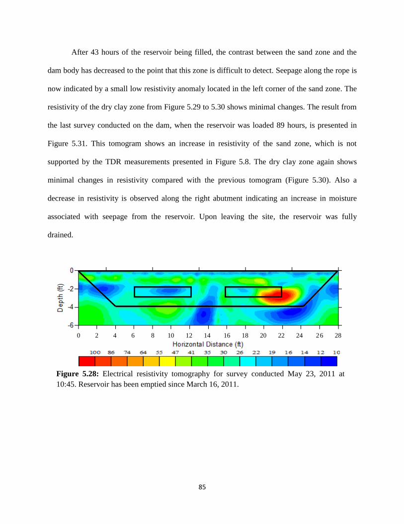
85

After 43 hours of the reservoir being filled, the contrast between the sand zone and the

dam body has decreased to the point that this zone is difficult to detect. Seepage along the rope is

now indicated by a small low resistivity anomaly located in the left corner of the sand zone. The

resistivity of the dry clay zone from Figure 5.29 to 5.30 shows minimal changes. The result from

the last survey conducted on the dam, when the reservoir was loaded 89 hours, is presented in

Figure 5.31. This tomogram shows an increase in resistivity of the sand zone, which is not

supported by the TDR measurements presented in Figure 5.8. The dry clay zone again shows

minimal changes in resistivity compared with the previous tomogram (Figure 5.30). Also a

decrease in resistivity is observed along the right abutment indicating an increase in moisture

associated with seepage from the reservoir. Upon leaving the site, the reservoir was fully

drained.

0 2 4 6 8 10 12 14 16 18 20 22 24 26 28

Figure 5.28: Electrical resistivity tomography for survey conducted May 23, 2011 at

10:45. Reservoir has been emptied since March 16, 2011.

86

0 2 4 6 8 10 12 14 16 18 20 22 24 26 28

Figure 5.29: Electrical resistivity tomogram for survey conducted May 24, 2011 at 9:35.

Reservoir has been filled for 20.5 hrs.

0 2 4 6 8 10 12 14 16 18 20 22 24 26 28


Reservoir has been filled for 43 hrs.


Reservoir has been filled for 89 hrs.

0 2 4 6 8 10 12 14 16 18 20 22 24 26 28

87

iv). August 2011 trip

The fourth trip made to Stillwater, Oklahoma was in early August 2011. The

environmental conditions before arriving at the HERU facility included very little rainfall and

extreme temperatures (90-100 degree Fahrenheit). This drought-like condition caused the

embankment dam to dry out which resulted in excessive cracking. Photographs of these cracks

along the surface of the dam are presented in Figure 5.32. These cracks reached depths of

approximately 2 feet and complicated the ERT surveying.

Figure 5.32: Cracking of embankment

These cracks made the placement of the electrodes difficult and created poor contact

resistances between the electrode and the ground resulting in noisy data.

The results from the first survey conducted in the August 2011 trip are presented in

Figure 5.33. The reservoir for this survey had been emptied for about 2 months. The high

resistivity anomaly across the tomogram represents the cracks along the surface of the crest and

surface drying. This anomaly reaches a depth of about 2 feet at several locations which are

consistent with the depth of the cracks. The TDR sensors plots presented in Figure 5.8 and 5.9

88

support a general decrease in moisture in the dam. This is consistent with the generally higher

resistivity of the dam. Approximately thirty minutes after the reservoir was loaded,

uncontrollable seepage associated with the cracking was observed. The flow of water through the

dam posed concern regarding its stability. It was decided to unload the reservoir. Instead of

conducting surveys with the dam reservoir completely filled, surveys were conducted with the

reservoir loaded at 1, 2, and 3 foot water levels respectively. The purpose of filling the reservoir

to these specific water depths was to determine if seepage can be detected at different heights of

water in the reservoir. The initial loading of the reservoir that occurred on August 1, 2011 filled

the cracks with water, causing the moisture level of the dam to increase. This increase can be

confirmed by abrupt changes in the TDR readings. The increase in moisture reduced the

influence of the cracks on the resistivity measurement (Figure 5.34). Also the tomogram in

Figure 5.34 shows an increase in moisture around the abutments which is associated with

seepage from the reservoir. This seepage around the abutments has been observed in tomograms

from previous surveys. Changes in electrical resistivity in the tomograms shown in Figure 5.34

to 5.36 are minimal. The sand zone and the dry clay zone are not detected in any of the

tomograms during the August trip; also detection of seepage at different reservoir heights was

unable to be detected. This is related to the cracks along the dam which resulted poor survey

conditions and noisy data collection.

89


12:45. Reservoir has been emptied since May 27, 2011.

0 2 4 6 8 10 12 14 16 18 20 22 24 26 28

0 2 4 6 8 10 12 14 16 18 20 22 24 26 28

Figure 5.34: Electrical resistivity tomogram for survey conducted August 2, 2011 at 7:45.

Reservoir was filled to a height of 1.5 feet.

0 2 4 6 8 10 12 14 16 18 20 22 24 26 28


11:45. Reservoir was filled to a height of 2.6 feet.

1018325595165288500

1018325595165288500

1018325595165288500

90

5.6 Summary

A quarter-scale experimental dam was constructed with internal compromised zones

susceptible to seepage and piping. Electrical resistivity tomography was used to monitor internal

changes in the dam related to both seasonal variation and loading/unloading the reservoir.

The largest observed changes in the electrical resistivity of the dam occurred during the

first cyclic loading and during the extreme temperatures/drought of the summer. A newly

constructed dam has a dryer material (below field capacity) and is susceptible to larger increases

in moisture associated with the first loading of the reservoir. This larger change in moisture will

result in a larger change in resistivity. The drastic changes in electrical resistivity of the dam

during the summer months were caused by the extreme temperatures and lack of precipitation,

causing the clay to dry out and crack. The cracking caused difficulty in field setup and obtaining

quality measurements. The results obtained in the rainy season of March and May were very

similar. Both of these trips showed that the when the dam had allowable time to drain from

previous reservoir loading, the detection of the sand zone was possible, but the detection of the

dryer clay zone was not. When the dam was subsequently loaded and sufficient time was allowed

for adequate seepage, the detection of the sand zone became more difficult. The opposite was

0 2 4 6 8 10 12 14 16 18 20 22 24 26 28


14:00. Reservoir was filled to a height of 3.2 ft.

1018325595165288500

91

true for the dryer clay zone. The seepage causes a further decease in resistivity of the clay zone

and was then detectable as a zone of lower resistivity.

92

6. CONCLUSIONS

The National Inventory of Dams approximates that there are about 75,000 (87%) earthen

embankment dams across the United States (NID, 2009). The majority of these dams have

approached their design life of 50 years and will require thorough inspections to assure their

integrity and the safety of the downstream population. The traditional approach to assess a dam’s

performance is through visual inspection but internal failure mechanisms will be missed.

The second leading cause of dam failure, seepage and piping is an internal problem that

involves water from the reservoir flowing through the dam body. Visual inspections may not be

able to detect this until it has progressed to an advanced stage. Electrical resistivity tomography

is a non-destructive geophysical method that can provide internal information on the

embankment which can help detect problems related to seepage and piping.

In order to effectively use the results from ERT, an understanding of how the resistivity

of materials used to construct dams (clays, silts, sand, etc.) is required. Several parameters affect

resistivity including: porosity, saturation, pore fluid resistivity, and clay content. These

parameters can be inserted into empirical formulae, such as Archie’s law or Waxman Smits, to

estimate expected resistivities.

Forward modeling can be performed using software to help validate electrical resistivity

tomography for solving a particular geological or environmental problem. Also, these models

93

help determine the strategic survey planning parameters (electrode configuration and electrode

spacing) to obtain optimal data collection. An understanding of the resistivity of the subsurface

and the size and depth of the zone being investigated, aids in constructing the forward models.

These models ultimately determine whether or not the zones can be detected or resolved in the

collected data sets in order to locate them in the ground. The models are generally generated

before conducting resistivity surveys; this helps reduce lengthy field time which reduces costs.

As part of this research, a quarter-scale earthen embankment dam was constructed at the

USDA-ARS HERU research facility with known internal flaws. These flaws were designed in

order to be susceptible to seepage. Time-lapse electrical resistivity tomography (ERT) surveys

were conducted on the dam over a period of a year. Based upon the results from ERT surveys

conducted on the experimental dam, it is concluded that this nondestructive geophysical method

is effective in identifying weak zones in an earthen dam that would be susceptible to seepage.

Furthermore, the results show that ERT surveys conducted on embankment dams shortly

after construction can be utilized to validate the construction techniques (compaction of dam

materials at consistent moisture content). Since most dams fail during the first reservoir loading,

conducting these ERT surveys would assist in determining the integrity of the dam and provide

evidence that it is safe to load the reservoir. The first survey should be conducted soon after

completion because subsequent weathering makes the detection of undercompacted zones more

difficult.

Conducting time-lapse ERT surveys over the course of the seasonal year indicates that

the dam’s internal structure changes due to weather. According to the results illustrated in

Chapter 5, the dam has a lower resistivity during the spring months and a higher resistivity

during the summer months. According to the Mesonet recordings, increased amounts of rainfall

94

are associated with the spring months and allow for a more conductive dam. This will result in a

lower overall resistivity of the dam. The amount of precipitation during this time produces a

higher level of contrast between the compromised zones and the dam body which makes their

detection easier. During the summer months, drought like conditions may occur (decreased

rainfall and extreme temperatures). These conditions cause the embankment to dry out and crack.

The survey data related to these environmental conditions is noisy. Noisy data makes detection

of compromised zones extremely difficult to impossible.

Changes in tomograms associated with a loaded reservoir are detected using time-lapse

electrical resistivity tomography. These changes are caused by seepage water from a loaded

reservoir and appear in the tomograms as low resistivity anomalies. Four trips were made to the

research site in which surveys were conducted on the dam with a loaded reservoir. The results

from these time-lapse surveys show that the largest changes occur at the location of the

compromised zones. In the tomograms presented in Chapter 5, the largest changes are occurring

in the dry clay zone, sand zone, and along both of the abutments and are supported by TDR

measurements. Evidence recorded shows that after a given amount of time (usually a period of

three to four days); the seepage water was eventually visible out the downstream side of the dam

in these specific regions. This evidence helps validate the ERT method in detecting seepage

inside a dam.

The best possible time to detect compromised zones inside an embankment dam using

electrical resistivity tomography is when the dam has a higher conductivity caused by increased

precipitation. This helps make the dam more conductive which allows for an increased contrast

between the dam and the zones resulting in their detection. Another best possible time to locate

weak zones in a dam is when the reservoir is full and has had adequate time for seepage to occur.

95

This will help increase the saturation of these higher porosity zones ultimately causing their

resistivity to be lower than the background (dam body) causing an increase in their contrast

leading to their detection.

In conclusion, ERT is a geophysical method that can detect areas in a dam that are

vulnerable to seepage and piping. Future work using ERT include conducting surveys on a full

scale dam that has known seepage problems. This will help further validate the method on real

world applications regarding seepage detection. Also comparing results from additional

geophysical methods that are sensitive to moisture changes, such as electromagnetics (EM) or

self-potential (SP), can help complement ERT results in locating seepage. Also further analysis

should be conducted in order to gain more of a quantitative analysis regarding the time-lapse

ERT results. This may include differencing the tomograms acquired from the trips to gain

information regarding the changes in resistivity of the zones/abutments associated with the

seasonal variations and changes related to a loaded reservoir.

96

BIBLIOGRAPHY

97

Advanced Geosciences Inc., (AGI), 2009. http://www.agiusa.com/index.shtml.

Al-Fares, W., 2011. Contribution of the geophysical methods in characterizing the water leakage

in Afamia B Dam, Syria. Journal of Applied Geophysics 75, 464-471.

Association of State Dam Safety Officials, (ASDSO), 2009.

http://www.damsafety.org/news/?p=412f29c8-3fd8-4529-b5c9-8d47364c1f3e.

Bedrosian, P. A., Burton, B. L., Powers, M. H., Minsley, B. J., 2012. Geophysical investigations

of geology and structure at the Mathis Creek Dam, Truckee, California. Journal of

Applied Geophysics 77, 7-20.

Cardimona, S., 2002. Electrical resistivity techniques for subsurface investigation. Department of

Geology and Geophysics, University of Missouri-Rolla, Rolla, MO.

Department of Ecology, the State of Washington, 2007.

http://www.ecy.wa.gov/programs/wr/dams/failure.html.

EarthImagerTM

2D Resistivity Inversion Software Instruction Manual, Version 2.4.0, 2007.

Griffiths, D. H., King, R. F., 1965. Applied Geophysics for Engineers and Geologists. Pergamon

Press, Oxford.

Hanson, G. J., Hunt, S. L., 2007. Lessons learned using laboratory jet method to measure soil

erodibility of compacted soils. Applied Engineering in Agriculture 23, 305-312.

Kearey, P., Brooks, M., 1984. An Introduction to Geophysical Exploration. Blackwell Science,

Oxford.

Loke, M. H., 2011. Tutorial : 2-D and 3-D electrical imaging surveys.

http://www.geotomosoft.com/downloads.php.

Mavko, G., Mukerji, T., Dvorkin, J., 1998. The Rock Physics Handbook. Cambridge Univ.

Press, Cambridge.

Minsley, B. J., Burton L. B., Ikard, S., Powers M. H., 2011. Hydrogeophysical investigations at

Hidden Dam, Raymond, California. Journal of Environmental and Engineering

Geophysics 16, 145-164.

National Inventory of Dams (NID), 2009.

http://geo.usace.army.mil/pgis/f?p=397:5:0::NO.

Palacky, G. J., 1987. Resistivity characteristics of geologic targets. Electromagnetic Methods in

Applied Geophysics 1, 53-129.

Pozdnyakova, L.A., 1999. Electrical Properties of Soils Ph.D. Thesis, University of Wyoming.

http://www.agiusa.com/index.shtml

98

Samouëlian, A., Cousin, I., Tabbagh, A., Bruand A., Richard G., 2005. Electrical resistivity

survey in soil science: a review. Soil and Tillage Research 83, 173-193.

Sjödahl, P., 2006. Resistivity Investigation and Monitoring for Detection of Internal Erosion and

Anamolous Seepage in Embankment Dams. Ph.D. Thesis, Lund University.

SuperStingTM

with SwiftTM

Automatic Resistivity and IP System Instruction Manual, 2006.

Waxman, M. H., Smits L.J. M., 1968. Electrical conduction in oil-bearing sands. Society of

Petroleum Engineers Journal 8, 107-122.

Weller, A., Cahn, T., Breede, K., Trong Vu, N., 2006. Multi-electrode measurements at Thai

Binh Dikes (Vietnam). Near Surface Geophysics 4, 135-143.

99

APPENDIX

100

Table A.1: Schedule for surveys conducted on embankment dam

Survey Date Survey Time State of Dam Array Type Electrode Spacing

October 13, 2010 15:45 Empty Res dipole-dipole 0.15m

October 13, 2010 6:25 Empty Res Inverted Sch. 0.15m

October 14, 2010 7:00 Empty Res Wenner 0.15m

November 29, 2010 11:30 Empty Res dipole-dipole 0.28m

November 29, 2010 13:55 Empty Res Inverted Sch. 0.28m

November 29, 2010 16:50 Res Full 0 hrs dipole-dipole 0.28m

November 29, 2010 17:20 Res Full 0.5 hrs Inverted Sch. 0.28m

November 30, 2010 10:45 Res Full 18 hrs dipole-dipole 0.28m

December 1, 2010 13:00 Res Full 44 hrs dipole-dipole 0.28m

December 1, 2010 13:55 Res Full 45 hrs Inverted Sch. 0.28m

December 2, 2010 10:40 Res Drained dipole-dipole 0.16m

December 2, 2010 11:30 Res Drained Inverted Sch. 0.16m

December 2, 2010 13:45 Res Refilled 0 hrs dipole-dipole 0.16m

December 2, 2010 14:40 Res Refilled 1 hr Inverted Sch. 0.16m

March 14, 2011 9:20 Empty Res dipole-dipole 0.15m

March 14, 2011 10:00 Empty Res Inverted Sch. 0.15m

March 14, 2011 14:40 Res Full 1 hr dipole-dipole 0.15m

March 15, 2011 10:30 Res Full 21 hrs dipole-dipole 0.18m

March 15, 2011 11:05 Res Full 21.5 hrs Inverted Sch. 0.18m

March 15, 2011 11:45 Res Full 22 hrs Schlumberger 0.18m

March 15, 2011 14:15 Res Full 24.5 hrs dipole-dipole 0.18m

March 15, 2011 14:50 Res Full 25 hrs Inverted Sch. 0.18m

101

March 16, 2011 10:25 Res Full 44.5 hrs dipole-dipole 0.18m

March 16, 2011 11:00 Res Full 45 hrs Inverted Sch. 0.18m

March 16, 2011 11:50 Res Full 46 hrs Schlumberger 0.18m

March 16, 2011 14:40 Res Full 49 hrs dipole-dipole 0.18m

May 23, 2011 10:45 Empty Res dipole-dipole 0.18m

May 23, 2011 13:00 Res Full 0 hrs dipole-dipole 0.18m

May 24, 2011 9:35 Res Full 20.5 hrs dipole-dipole 0.18m












August 1, 2011 12:45 Empty Res dipole-dipole 0.18m

August 2, 2011 7:45 Res Filled to 1.5ft dipole-dipole 0.18m



102

VITA

Jared Case enrolled at the University of Mississippi in the fall of 2005. As an

undergraduate student, Jared worked as an intern for the National Aeronautics and Space

Administration (NASA) at the Glenn Research Center (GRC) in Cleveland, Ohio, the

Engineering Research and Development Center (ERDC) in Vicksburg, Mississippi, and lastly for

the National Center for Physical Acoustics (NCPA). He obtained a Bachelor’s of Science in

Civil Engineering (B.S.C.E.) in May 2010 and decided to continue his education at the

University of Mississippi by enrolling in their graduate school program. He obtained a Master’s

in Engineering Science with a concentration in Civil Engineering (M.S.) from the University of

Mississippi in May 2012 and will be employed by Halliburton upon graduation.

Inspection of Earthen Embankment Dams Using Time Lapse ...

Documents

Transcript of Inspection of Earthen Embankment Dams Using Time Lapse ...