HD28.M414

no.'64i4

-Tl

Inspection for Circuit Board Assembly

Philippe B. Chevalier

andLawrence M. Wein

WP# 3465-92-MSA September, 1992

MASSACHUSETTS

INSTITUTE OF TECHNOLOGY50 MEMORIAL DRIVE

CAMBRIDGE, MASSACHUSETTS 02139

Inspection for Circuit Board Assembly

Philippe B. Chevalier

andLawrence M. Wein

WP# 3465-92-MSA September, 1992

MIT. LIBRARIES' CT 2 1992]

REUcivB;

INSPECTION FOR CIRCUIT BOARD ASSEMBLY

Phillipe B. Chevalier

Operations Research Center, M.I.T.

and

Lawrence M. Wein

Sloan School of Management, M.I.T.

Abstract

Several stages of tests are performed in circuit board assembly, and each test consists

of one or more noisy measurements. We consider the problem of jointly optimizing the

allocation of inspection and the testing policy: that is, at which stages should a board

be inspected, and at these stages, whether to accept or reject a board based on noisy

test measurements. The objective is to minimize the exp(^cted costs for testing, repair,

and defective items shipped to customers. We observe that the optimal testing policy

is very sensitive to some input data that is extremely hard to estimate accurately in

practice. Hence, we do not pursue an optimal solution, although it could be calculated

with considerable effort. Rather, we derive a closed form testing policy that is Pareto

optimal with respect to the expected number of type I and type 11 errors, and then find

an optimal inspection allocation given this testing policy. We also describe an application

of the model to an industrial facility that is using it, and find that the proposed policy

significantly improves upon the facility's historical policy.

September 1992

INSPECTION FOR CIRCUIT BOARD ASSEMBLY

Philippe B. Chevalier

Operations Research Center, M.I.T.

and

Lawrence M. Wein

Sloan School of Management, M.I.T.

1. Introduction

This paper considers the problem of inspection in a circuit board assemblj' plant, which

came to our attention while working with a Hewlett-Packard facilitj-. Recent technological

advances have given rise to circuit boards of increasing complexity, and consequentlj' testing

has become one of the most challenging aspects of circuit board manufacturing. Inspection

costs can account for over half of the total manufacturing cost, and hence optimizing the

utilization of inspection resources is a crucial task.

The assembly of circuit boards is performed in a single manufacturing stage, which

is followed by several successi\'e inspection stages. Assembled circuit boards haA'e to be

inspected for manufacturing defects and defective components. The inspection process at

each stage includes three different activities: testing, diagnosis and repair. In testing, one

or more measurements are taken from a board, and a decision is made whether to accept or

reject a board. The defect on a rejected board is identified during diagnosis, and is corrected

during repair. Diagnosis is often the most difficult and time consuming task and the degree

of difficulty depends on the board type and the type of test that is performed. The main

focus of this paper is on testing, and henceforth repair refers to diagnosis as well as repair.

The attractiveness of a test depends on its cost, diagnostic power, coverage and mea-

surement errors. The cost for performing a test on a particular board depends on the type

of that board. The diagnostic power of a test is the amount of information that a test

1

provides for diagnosis, and it strongly influences the time required and the cost for a repair.

Defects are considered to be of different types, and the coverage of a test refers to the range

of defects that can be detected, and the extent to which they can be detected. For example,

in Figure 2, the defect types linked to defective assembly, such as opens and shorts, are very

well covered at the first inspection stage, whereas defective components are much harder to

detect and some components can only be detected at the last inspection stage. The outcome

of a test is one or more measurements, and the accuracy of these measurements determines

the prevalence of type I (false reject) and type II (false accept) errors.

We consider two interrelated decisions. The first decision is to decide at which stage(s) to

inspect a board; this problem is known in the literature as the inspection allocation problem.

At the stages where inspection is performed, the testing policy decides whether to accept

or reject each board based on the noisy measurements obtained from the test. The joint

decision of inspection allocation and testing will be referred to as an inspection policy. The

optimization problem is to find an inspection policy to minimize the total expected cost,

which includes costs for testing, repair and defective items shipped to customers. Lince we

assume that every defective board is repaired, no scrapping cost is included.

We make one crucial assumption that allows for a tractable anah'sis: the probability

distribution of the true value of a measurement at a particular stage is independent of

the inspection policy employed at previous stages. If the measurement under consideration

is trying to detect a type i defect, then one would expect that the presence of previous

inspections related to type i defects, as well as the use of tight acceptance intervals for these

tests, would lead to a narrower distribution of the true measurement value. The exact nature

of this dependency can be very complex since the same quantity is not measured at different

stages. The quantities measured at later stages are typically an aggregation of quantities

measured earlier, and the nature of this aggregation might either dampen or amplify the

effect of a defect. Even if a model of this dependency was developed, data collection would

be extremely difficult. Typically, the only available data is the noisy measurements under the

2

existing inspection policy; experiments would probably need to be performed under various

inspection policies to gather the necessary data. In our case study, the derivation of an

optimal testing policy was primarily an issue at in circuit testing (many of the other tests

had binary results), which is the first test undertaken, and consequently the independence

assumption was not an issue.

We encountered a formidable obstacle to implementing an optimal solution to this prob-

lem: the optimal testing policy is very sensitive to the probability distributions of the

measurement errors, which are exceedingly difficult to estimate to the required degree of

precision. Hence, the considerable computational effort required to derive the optimal in-

spection pohcy did not appear to be worthwhile. Instead, we found a testing policy with

several important features: (i) the cutoff limits for acceptance and rejection that charac-

terize the testing policy are expressed in closed form; consequently, the test engineers at

Hewlett-Packard found the policy intuitively appealing, and easy to understand and use; (ii)

the policy is Pareto optimal with respect to the expected number of type I and type II errors

incurred; and (iii) the cutoff limits should be close to the optimal cutoff limits if reasonably

accurate parameter estimates are used.

Given this testing policy, the optimal inspection allocation policy is then easily cal-

culated. Since the cardinahty of the action space is small and the dimensionality of the

continuous state space can be large, we employed an exhaustive search procedure instead of

a dynamic programming algorithm.

The paper contains a short case study of the Hewlett-Packard facility, where oui- model

is being applied. The case studj' includes a description of the facility, the methodology for

gathering the data, which has been disguised, and the proposed policy. Relative to this

facility's historical inspection policy, our limited numerical results suggest that the proposed

allocation policy can reduce total inspection costs by 10-20%, and the proposed testing policy

can reduce costs by roughly 5%. The proposed inspection policy is in the process of being

implemented, and we are not yet in a position to report on the cost reduction realized by

3

the facility.

Two by-products of our analysis are of significant practical value. First, we determine

the cost reduction that would be achieved by reducing the measurement noise of the test

equipment. This quantity can help circuit board manufacturers evaluate new test equip-

ment, and can assist test equipment manufacturers focus their R&D efforts and market their

equipment. Although inspection is necessary in the context of circuit board assembly, qual-

ity improvement efforts are also vital to a company's success. We also derive the marginal

benefit from reducing various types of defects. These quantities can be used to focus quality

improvement efforts in an economic fashion.

Many papers have been published on the optimal allocation of inspection in multistage

serial systems. Early studies on this problem (see, for example. White 1966 and I indsay

and Bishop 1967) assumed perfect inspection (i.e., no type I or type II errors). Later papers

allowed for imperfect inspection (Eppen and Hurst 1974, Yum and McDowell 1981 and

Garci^-Diaz et al. 1984), where cne determines the number of times that a test should be

repeated. A survey of work published on inspection allocation can be found in Raz (1986).

Recently, Villalobos et al. (1992) studied a dynamic version of the same problem, where

inspection of an item at a particular stage can depend on the result of the inspection of that

item at previous stages. Our paper appears to be the first to address the presence of distinct

defect types, the joint optimization of inspection allocation and testing, and the application

of a model to an industrial facility.

Section 2 presents a detailed formulation of the problem, which is then analyzed in

Section 3. A case study is presented in Section 4, and conclusions are drawn in Section 5.

2. Problem Formulation

A typical flow chart of the assembly of circuit boards is presented in Figure 1. The

main manufacturing stage is circuit board assembly, where all the components are soldered

onto the printed circuit boards. At the system assembly, the different boards are plugged

4

into the final product. The in circuit test takes a measurement from each of the individual

components soldered on a board, and the functional test assesses the response of a board to

simulated working conditions. At the system test, each board is tested as part of a complete

system. Many variants of the configuration displayed in Figure 1 are possible. For example,

there could be multiple levels of each test, or the system assembly step could be performed

in several stages, and a test could be performed on each subassembly; on the other hand,

some tests might not be present.

Printed CircuN

Boards

Circuit BoardAssembly

In Circuit

Test

System

Test

Figure 1 . Flow chart of circuit board assemblj'.

As mentioned earlier, an important characteristic of each test is its coverage. We will

assume that for each type of defect, the successive tests that are performed on the circuit

boards have an increasing coverage. Figure 2 illustrates this property, which we call hierar-

chical test coverage, for the example introduced above. Since they cover more defect types,

successive tests tend to be more complex and more expensive to perform. However, as the

complexity of the test increases, the precision of the information obtained from the test

decreases. Consequently, type I and type II errors are more prevalent, and diagnosis takes

longer and has to be performed by more qualified personnel. The hierarchical assumption

in test coverage holds for the circuit board assembly systems we have encountered. This

assumption also holds in traditional manufacturing settings, where additional work is per-

formed between successive tests, and each test measures the cumulative functionahty of the

manufactured item.

Main Defect type Inspection Stage

Captured at inspection

Defective Assembly

• Defeaive ComponentIn Circuit Test

• Defeaive Component Functional Test

• Incompatible Component Syiem Test

Figure 2. Hierarcliical test coverage.

In this section, the problem is formulated for a single board type in isolation. In Sec-

tion 3.3 we discuss how to account for the dependencies between different board types.

A test consists of a series of up to several thousand measurements. These measurements

relate to different components on a board, or to different aspects of the overall functional

performance of a board. Most of these measurements are subject to some noise, and this

measurement error is quite sensitive to small changes in the board design or the manufac-

turing process. The testing policy at a stage specifies an interval for each measurement

such that a board will be accepted if every measurement lies inside its interval, and rejected

otherwise. The presence of measurement errors makes it impossible to completely eliminate

type I and type II errors. Larger intervals will lead to the acceptance of more boards, which

will reduce the number of good boards falsely rejected but increase the number of defective

boards falsely accepted. Similarly, smaller intervals will have the opposite effect.

For tests that have binary results, only one testing policy needs to be considered. Ex-

amples of such situations are systemwide functional tests and tests for opens and shorts.

For the purpose of generality, we allow the model to have a choice of testing policies at each

6

stage. However, the model easily accommodates the case where the set of possible testing

policies at one or more stages is reduced to a single policy.

We assume that each measurement can detect only one type of defect. For i = 1, . ..

, /

and n = 1, . ..

, TV, let A',„ be the number of measurements taken at stage n that detect type

i defects, and let v^f. be the value obtained from the k*^^ measurement for type i defects at

stage n. Then

where f'^^ is the true measurement value and e,„fc is the measurement error. We assume

that these two random variables are independent, and that the measurement errors are

independent across different measurements. These independence assumptions appear to hold

in practice. As mentioned in the Introduction, we also make the simplifying assumption that

the distribution of i^'^^. is independent of the inspection pohcy at previous stages.

Let Pink{^) be the conditional probability that the true value v]^). is inside Gmk. which is

the interval in which the true value should be for the proper functioning of the board, given

the measurement value; that is,

p^ir) = Pt[vI, e G'.nfcI C, = ,r].

The function p,nk{-f) can be expressed solely in terms of the problem inputs as

/ ^ _ ^G,„, g<nA-(j- - y)^,nk(y) dy

J_oc e,„t(3-- yK:nk{y)dy

where ^inki^) 's the probability density function of the true value of the quantity measured,

and e,„t(x) is the density function of the measurement error.

The testing policy for defect type i at stage n is defined by T,n = {(L,„i,-.U,nk)-k =

1, . ..

, A',„}, where the A-"^ measurement for type i defects at stage n is accepted if it lies

inside [L,„fc,t/,„t]. Define

Q,nk{L,nkJ^mk) = Pi" ''La- € G,nk and V^^i^. ^ [i,nkA',nk

and

l3,nk{L,nk.U,nk) = Pr {l^k ^ G^nk and V^^^ ^ [L,nkJhnk]] ,

where Q,nk{I^ink,f^'ink) is the probability that the measurement is rejected although the true

value of the component is good, and ^inkiL,nki U,nk) is the probability that the measurement

is accepted while the true value of the component is bad. If we let f,nk{^) be the density

function of the measured values, then

P,nk{x)frnk{x)dx + P,nk{x) f,nk{x) dx (2)-OO JU,nk

and

/3ink{L,nk-lhnk) = (\ - f^nki^-)) f>nk(x) dx

.

(3)

Let Q,n(T,„) be the expected number of false defects of type i per board at stage ?i under

testing policy T,„, and lei /ij„(r,n) be the expected number of defects of type ?' present on a

board at stage ?? that are not detected at that stage. It follows that

Olin{T,n) = X! Ihnk{-r).f,nk(-r)dx + / pt„i,{x)f,„i,(x}dx (4)

and

An(r,„) = 2^ / {I - Pznk{3-))f>nk(x)dx. (5)k=l •^^'"'•

For technical reasons that will become apparent later, we assume that Pmki-''^) and /,„t(x)

are continuous unimodal functions for all i, n and k.

In addition to deciding upon a testing policy, we also need to choose the inspection

allocation policy at each stage, which specifies whether or not to test the boards at that stage.

Notice that additional stages can be artificially added to consider partial testing options at

particular stages. The objective is to minimize the total expected cost of testing, repair, and

defects leaving the plant; this total cost will often be referred to as the total inspection cost.

We consider a per unit testing cost /„ at stage ??, which typically includes operator time,

test engineering, equipment depreciation and maintenance, and various overhead costs. A

possible benefit, or negative cost, of testing is that it will lead to quicker learning and hence

process improvements; however, in our case study, we did not attempt to incorporate this

benefit into the per unit testing cost. Also, no fixed testing cost is included in the model.

The repair cost r,„ is the total cost incurred to diagnose and repair a type i defect on a

board at stage n. We assume that all defective boards are repaired, and that the same repair

cost is incurred, whether the defect is a real defect or a false defect. The cost / of a defect

on a board that leaves the plant includes the cost of a field repair, the cost of the analysis

and repair of the defective board that comes back to the plant, and a cost measuring the

customer's loss of goodwill. We assume that the cost is per defect and not per defective

system, which simplifies the analysis. However, if there are two or more defects in a system,

then it is unlikely that these defects would be detected by the customer at the same time.

Moreover, since the number of defects leaving the plant is very low, multiple defects on the

same system are very unlikely; consequently, the results obtained would be very similar if a

cost was incurred per defective system. We also assume that the cost / does not depend on

the type of defect on a board. Although the more general case can be easily accommodated,

this assumption seems practical, since the costs of lost goodwill and visiting the repair site

dominate the other costs, and are independent of the defect type.

As a consequence of the hierarchical test coverage assumption, more defects become

detectable at each inspection stage. We model this as if, on average, d,„ new defects of type

i appear per board at stage n. Let 6,n denote the average number of defects of type / per

board that leave stage n. Notice that 6,^ depends on the inspection policy at all earlier

stages, and cf,„ and 6,„ are expected values. The distributions of the random variables from

which these expected values are derived do not matter because all the costs in the model are

linear and dynamic allocation policies (i.e., policies where the decision to inspect depends

upon what was observed earlier on the board) are not considered. If inspection is performed

at stage n and testing policy T,,, is used, then the expected cost of testing and repair at that

stage is

/

!=1

and the expected number of defects of type ?' per board leaving stage n is

On the other hand, if no inspection is performed at stage n, then no cost is incurred at that

stage. The expected number of type i defects per board leaving stage n in this case is

The optimization problem is to decide whether to inspect at each stage, and if so. what

testing policy Tin to use, if such a choice exists, to minimize the expected total inspection

cost,

N / I \ I

Hi'" + X] ''" (^'."-1 + d,n + 0,n(T,n) - l3,n(Tin)) + /^ ^tA'- (6)n=l

V

i-1 / i=l

3. Analysis

In this section, we analyze the problem formulated in Section 2. The testing problem is

addressed in Seciion 3.1 and the inspection allocation pohcy is numerically derived in Section

3.2. Various extensions of the basic problem are described in the last three subsections.

3.1. The Testing Policy

This subsection contains three main results. First, we derive a set of testing policies

that is optimal with respect to the tradeoff between the expected number of type 1 and

type II errors per board in the sense of Pareto optimahty (i.e., it is impossible to reduce

one quantity without increasing the other). This result enables us to restrict our attention

to these policies when searching for an optimal testing polic\'. Second, three rather weak

additional assumptions are made to sharpen the first result. However, we observe that the

optimal testing policy is very sensitive to certain input data that are difficult to estimate

in practice. Hence, we conclude this subsection by proposing a closed form policy that is

Pareto optimal and easy to implement and understand.

10

The minimum expected total inspection cost from stage n until exiting the plant, which

is denoted by Jn{^\n^^2ni- • i^/n)i satisfies the dynamic programming optimality equations

Jn{pi,p2,---,Pi) = Min Jn + \{P\ + dxn,p2 + <^2n,-- -,/>/ + <^/n),

/„ + min«=1

(7)

and

+ J„+ l(/9ln(r.n),^2n(7^.n), • •, /^/nC^.n))

Jn+i{PuP2,- ,Pi) = IYIP'^1=1

for n = 1 , A'

,

(8)

where {p\,p2,- ,Pi) are dummy variables.

The second minimization in (7) can be rewritten more concisely as

min|/!„(Qi„(r;„),a2„(r,„), . . .,aj„{T,n)) + 5n(/3i„(r,„),/32„(r,n), /3/„(r,„))}. (9)

where

and

/i„(.ri,.T2,...,.r/) = J2 x,r,

1=1

9n{x\,X2,. . . ,xi) = J„+i(,ri,a-2,. . . ,.17) + '^{p, + d,„ - x,)r,„.

:io)

(ii:

l:=l

If Q',n(T,„) and l-^in{T,„) in (9) are replaced with the expressions obtained in equations (4)-(5),

then the derivative of this function with respect to the upper acceptance limit (',„;,. is

- -7^(Q^ln,0'2nv • • ^0:in)Pink{Uink)finkiU,nk)

r\

+ Tr^(/?ln,/?2n,- • • ,/^/n) (1 " P,nk{l',nk)) f,nk{l'n,k)<OX,

where, to simplify notation, a,„ stands for Q,n(7',n) and /?,„ stands for f3,„{T,n). This expres-

sion equals zero if

l^{01nJ2n,...,l3ln)(12)

The second derivative of the objective function (9) will be positive if f'ni,iU,nk) < and

P'inki^^'nk) < 0- One would expect the second order conditions to hold, since the upper

limit is at a point where both the frequency of measurement and the probability that a

measurement corresponds to a valid board are decreasing.

The same argument can be used to show that the optimal lower acceptance limit satisfies

Pink[^,nk} - ^T- X , da„,^ n TT^' U<JJ

The second derivative of the objective function (9) will be positive if fink{L>tnk) > and

P'inki^^rik) > 0. Again, the second order conditions are consistent with our intuition.

From the definition of /;„ and g„ in (lO)-(ll), it follows that

-7^— (oin,02„,.. . ,a/„) = r,„ (14

and

^(An,/?2nv,/^/n) = ^"^(/^In, /^2nv • • ,/^/n) " ?m. (15)

OX, dpi

Equations (12) and (13) now bpcom^"

j^

.

P,nk{L,nk) = P,nkif-',nk) = 1 " dj ^, , -, T ;—T (16)

^if^mjhn /i/n)

This expression has an intuitive meaning: the probability that a component is bad at the

acceptance and rejection cutoff points should be equal to the marginal cost of a false rejection

divided by the marginal cost of a false acceptance. As this cost ratio increases, it becomes

less costly to accept parts, and the acceptance region is increased. Notice that the right side

of (16) is a constant for each measurement k = 1, . . . /\r,„, which we denote by Ctn- The set

of Pareto optimal testing policies can be generated by letting C,„ vary from to 1.

The existence of lower and upper limits L,nk and Umk satisfying (16) is guaranteed by

the continuity and unimodality assumptions of /,nt(-T) and p,nk{^) stated in Section 2. We

will not pursue weaker necessary and sufficient conditions for the existence of these optimal

upper and lower hmits, since in our case stud}' these functions will be modeled b}' Gaussian

density functions that satisfy the necessary conditions.

12

We can let the right side of (16) vary between and 1, and use equations (1), (4), (5) and

(16) to compute in advance all possible optimal testing policies, and generate the functions

<^tn{C,n) and /S,„(C',n). As a result, the minimization in the dynamic programming recursion

(7) does not have to explicitly consider all possible testing policies, but only these two

functions. The nonlinear curve in Figure 7 in Section 4.2 shows an example of the tradeoff

curve of the expected number of type I errors per board (a,n(C,n)) versus the expected

number of type II errors per board (/?,„(C,„)) obtained by letting C,„ vary from to 1.

Since these quantities are independent of k^ the curve was derived by aggregating all several

hundred measurements (one per component) for this testing stage and defect type, which

was the in circuit test that detects defective components.

We now turn to a special case where the set of Pareto optimal testing policies can be more

explicitly described. This special case requires three further assumptions that are satisfied

in our case study and often hold in practice. First, we assume that the measurement noise

and the true value of the component being measured are normally distributed. It follows

that Pj„/:(.r) can be simplified to (all subscripts ,nk < " being dropped for better readability)

p{x)

]_/ . AGu -/<^)<^e + JGu + ft- r)(rh

__ AGt - fi^)aj + {G, + n, - .r)rr| .

2V'^ a,a^^2[al + al)' ""' ^

a,a^^2[al + a})^

(17)

where:

/if and Gf. are the expected value and the standard deviation, respectively, of the mea-

surement noise;

/i^ and cr^ are the expected value and the standard deviation, respectively, of the true

values of the component being measured; we will also refer to /i^ as the nominal value of

the component;

Gi and G'u are the lower and upper limits respectively of the interval G such that the

measured component is good if its true value lies inside it;

13

erf is the error function, erf(r) = -^ Jq e ' dt, which is plotted in Figure 3.

Figure 3. The error function.

We also assume that

and

|<7u — Gi> 1

CT^ > 3(7e.

(18)

19)

In quaUty management terminology, inequality (18) states that the machine capability index

is greater than 1; that is, the natural process range, 6a^, is smaller than the product spec-

ification range, IGj, — Gi\. Since many companies are currently striving for "Ga"' capability

(i.e., \Gu — Gi\ > 12cr^), (18) often holds in practice. Inequality (19) requires that the test

measurements be reasonably reliable.

By conditions (18)-(19), one term of the right side of equation (17) will always be equal

to 1 or -1, implying that p{L) = p{U) for any L and U such that

L = //^ + //e + (Gl - fi^)z (20)

and

U = //.^ + ft, + (Gn - /i^)-,

14

(21)

A

1 1

1 1 1

various components in our study and found that p(t) takes on values between 0.2 and 0.4.

Unfortunately, despite gathering a large amount of data in the case study, we will see later

that the 95% confidence intervals on the estimates used for p{x) are much wider than this

11.1% overestimate. For this reason, it is extremely difficult to obtain an optimal testing

policy that provides reliable performance.

Consequently, it does not seem worth the considerable effort required to derive the

optimal testing policy. Instead, we propose to simply set the lower and upper cutoff limits

to the middle points of the ascent and descent of p{x) in Figure 4; that is, we find the two

points such that p{x) = 0.5. These points, denoted by x/ and .r^, are derived by setting the

argument of either error function in (17) equal to zero, which yields

r/ = /'^ + /^ f (r;/-//4)(^^^) (22)

and

.r, = //,. + ^,, + (G, - //^)(^^^). (23)

.Although the value in the right side of (16) will often be closer to 0.9 than 0.' in

practice, the corresponding difference in the cutoff points will typically be dwarfed by the

inaccuracies in the measurement errors. Moreover, the cutoff points x/ and Xu have several

desirable features. Even if the parameter estimates are inaccurate, the testing policy (.r/,Xu)

is still Pareto optimal. Also, this policy is easy to find and can be expected to he close

to the optimal policy if the estimates used for p{x) are reasonably accurate. Furthermore,

since the testing policy is derived in closed form, it is intuitively appealing, and is very easily

understood and implemented by the test engineers. More specifically, expressions (22)-(2.3)

have the following intuitive meaning (consult Figure 4): the acceptance interval should be

shifted from the tolerance interval by the expected value of the measurement noise; the

tolerance on both sides should be multiplied by a factor that is the ratio of the sum of

variance of the true values of the component and the measurement noise over the variance of

the true values of the component. This ratio shows verj' clearly how the acceptance interval

16

is affected by the measurement noise. For these reasons, xi and Xu are used to define the

testing policy in the case study described in the next section.

3.2. The Inspection Allocation Policy

The Pareto optimal curves characterized by a,>i(C,„) and ^in{Cin) can be substituted

for a,„(T',n) and ^,n(Tin), respectively, into the dynamic programming optimahty equation

(7), and the optimal inspection allocation policy can be derived by solving the resulting

dynamic program. However, the optimal solution becomes very tedious to calculate, since

the functions a,„(C„) and fi,n[C,n) and the /—dimensional state space are continuous, and

/ is of moderate size. More importantl}', as pointed out in Section 3.1, the optimal testing

policy is difficult to reliably implement in practice, and the testing policy derived in (22)-(23)

has many desirable characteristics. Hence, we propose to use the testing policy defined in

(22)-(23) and then find the optimal allocation policy given this fixed testing pohcy. Under

this proposal, the dynamic programming equation (7) simplifies to

-^n(/'l,/52v,/'/) =Min J„ + \{p\-\- dxn,p2-\- din ,Pl + dl„),

I1

(24)

!= 1^

where q,„ and /3,„ are computed from equations (4)-(5) by setting the cutoff hmits L and ('

to xi and x^-

Solving (8) and (24) numerically requires a discretization of the /—dimensional state

space of incoming defects, and can be cumbersome in many cases. In contrast, an inspection

allocation policy that solves (8) and (24) can be found relatively easily by employing an

exhaustive search procedure over all 2^^ policies, as described below.

Let TTn represent the inspection allocation policy at stage n, and let H^ = (7i"i, 7r2, . . . , tt^)

denote the allocation policy for the line up to stage m. For i = 1, . ..

, / and m — 1, . .. , A',

define

l^im if I'm — inspection,

^. n = "

<^,.n„,_, + d„n if TT,,, = no inspection.

which is the expected number of defects of type i that leave stage m under poHcy \\,„- For

77? = 1,...,A'^, the cost cn,„ of allocation policy n„ is calculated from the cost cn„,_j of

allocation policy Tlm-i by

CUrr, = <

/

CUm-l +tm + Yl '^•mi^t.Urr^-i + d,m + Q,m " Am) if T^m = InSpection,

crim-i if ^m — no inspection,

where cx\^ = (f,_no = 0. The search procedure calculates the total inspection cost over the

entire line, which is given by cn^ + /IlLi ^xS\n^ f°r ^ 2^ policies.

3.3. Dependencies Across Different Board Types

Until now, we have been considering only one type of circuit board. If different board

types were completely independent, then all of our results would carry ovor. However, some

tests actually measure several board tj'pes together, in which case either all the board types

are tested or none are tested. Thus, the inspection allocation decisions taken independently

might yield an infeasible solution. For shared tests that are nonparametric (i.e., have l)inary

results), this dependence can be dealt with by employing a Lagrangian relaxation approach,

where the total cost of the test is split among the different board types such that the solutions

found independently coincide. To illustrate this approach, let us suppose that the total cost

of a test that covers two board types is i. We run the model for the board types independently

with the cost t split arbitrarily between the two types. If the decisions for the two types

agree, then the solution is feasible and optimal. If the solutions do not agree, then modify

the allocation of t by increasing the cost for the board type that is tested and decreasing

the cost for the board type that is not tested. The problem is solved again for both board

types, and if the solutions still do not agree, then we repeat the entire procedure until the

solutions agree. Due to lack of data, this procedure could not be applied in our case study,

and hence we are not in a position to report on the efficiency of any particular cost allocation

algorithm. Notice that this approach becomes almost impossible to use with a parametric

test, because the Lagrange multiplier must be a function of the testing policy that is used.

18

In the plant under study, the tests that measured more than one board type were the more

comprehensive system tests, and hence were nonparametric.

Congestion also leads to dependencies across board types: if too many board types

are tested at the same stage, then the testing load may be undesirably high at that stage.

Moreover, if many of these board types are not tested at the previous stages, then many

repairs will be required at that stage, which leads to additional work. At considerable com-

putational expense, queueing effects could be incorporated here by a Lagrangian relaxation

method similar to that described above, or by directly incorporating queueing costs (derived

from a product form queueing network, for example) into the objective function. We did

not pursue this avenue because the congestion effects at the Hewlett-Packard facility were

negligible. Readers are referred to Tang (1991) for an inspection allocation problem with

queueing costs.

3.4. Improved Testing Equipment

Our model explicitly takes into account the effect of measurement noise, which enables

us to determine the value of improved testing equipment that possesses lower measurement

noise. This issue is very important, since testing equipment is extremely expensive and

it is not clear, a priori, how a reduction in measurement errors affects the overall cost of

inspection.

To evaluate improved testing equipment in the context of our model, the new noise

parameters /Zg and a^ are substituted into equations (22)-('23) and the exhaustive search

procedure described in Section 3.2 is carried out. The optimal total inspection cost for the

new equipment can then be compared with the corresponding value for the old equipment.

An experiment was performed to illustrate the magnitude of the savings achievable with

more precise equipment. We assumed that a hypothetical new tester had a measurement

noise whose standard deviation was half of that of the current tester. For the in circuit

test that detects defective components in our case study, the tradeoff curve for the new and

19

original test equipment is pictured in Figure 5, which shows that both types of errors could

simultaneously be divided by at least two using the new equipment; the upper curve in this

figure is identical to the curve in Figure 7. If we assume similar error reductions for all

components on the board, then the reduction in total inspection cost is on the order of 5

percent.

0.05

0.01 0.02 0.03 0.04 0.05 0.06 0.07 0.03 0.09 0.1

a

New Test Equipment A Original Test Equipment

Figure 5. Reduction in testing errors.

3.5. Allocation of Quality Improvement Efforts

Engineering resources to work on quality improvements are limited, and consequentlj' it

is important to dedicate resources to projects that have the maximum impact. In a slightly

different context, Albin and Friedman (1991) show that the choice of the most valuable

project is not always straightforward. In particular, they show that the traditional Pareto

chart is not an adequate tool when defects are clustered. It is also possible that a Pareto

Chart would be misleading for the problem considered here, since different types of defects

are detected in different propoitions at different stages and hence the cost of different types

of defects can be very different.

20

If the inspection policy for all stages following n is fixed, then the derivative of Jj,+i with

respect to its i*'^ argument is a constant for each i. This constant is the marginal expected

cost of having one more defect of type i leave stage n and is easily calculated. Let q,rn be the

probability that a defect of type i arriving at stage m is detected at stage m. If we assume

that all defects of type i reaching stage m are equally likely to be detected, then

9.tm*'i,Tn — 1 "r O-im

The probability that a defect of type i leaving stage n is repaired at stage m > n is

( n '?''j(l -Qtm)-

As a result, the expected total inspection cost created by this defect is

dJnN m-1 A^

,o-(-)= E n 9=/ (i-9™)r™ + n <?''/

Hence, under any fixed inspection policj', this quantity is the marginal cost reduction ob-

tained from reducing type i defects at stage 7i.

Recall that the hierarchical test coverage assumption implies that more defects become

detectable at each inspection stage; this was modeled by assuming that, on average. d,„ new

type i defects appeared per board at stage ??. As a result, working on the root cause of type

i defects will simultaneously reduce the mmiber of type i defects appearing at every stage. If

we assume that the proportion of type i defects across the different stages does not change,

then the marginal cost from reducing type i defects is

Z^n=l dp, \ '"'"

2.^71= 1 "m

4. Case Study

We now describe the application of this model to the Hewlett-Packard facility. This

plant has N = 3 inspection stages as shown in Figure 1. Approximately -50 different board

21

types are manufactured at this facility, and these boards go into various models of a single

line of final products. The number of boards produced of each type is relatively low, ranging

from 1,000 to 10,000 per year. Hence, tests must be flexible in order to accommodate many

different board types. Figure 2 illustrates the basic structure of the tests performed. We

grouped the many different categories of defects that are used internally into 7 broad types,

based on their similarity for testing purposes. These seven categories are open and shorts,

missing or wrong components, defective components, two different soldering defect types

(one is much harder to detect than the other), miscellaneous, and testing problems. This

last category consists entirely of false defects, and occurs when a defect is thought to be

detected, but no problem can be found. Except for this last defect tj'pe, the number of

measurements for each stage and defect type, A',„, ranges from about 20 to several hundred.

The nature of the final product, which cannot be revealed, requires very strict tolerances

on the circuit boards and on their components, which partially explains why this facility cur-

rently tests all boards at all stages. The facility uses no consistent procedure for determining

testing policies, and the policy is highly dependent on the particular engineer in charge of

the test. The managers at this facility estimate that the total cost of inspection represents

about half of the total manufacturing cost.

It would be an enormous task to collect data and derive the proposed inspection policy for

all 50 board types. Instead, we applied our model in a very limited manner in order to exhibit

its effectiveness, and left the appropriate software with the Hewlett-Packard engineers, who

are carrying out the implementation. The data collection procedure is described in Section

4.1 and our results are given in Section 4.2.

4.1. Data Collection

Our model requires three different types of data. The first type is the cost parameters,

and the second concerns the occurrence of defects, and the coverage and reliability of each

inspection stage. The last and perhaps most difficult type of data to gather pertains to the

22

testing process.

Testing and repair are two activities that are closely linked, since they are performed

by the same people in the same work area. Their cost includes technician time, floor space,

equipment and overhead for management time. To allocate cost between these two activities,

we use estimates of the time that different engineers and technicians spend on each of these

activities. Both of these costs vary for each board type; in particular, they depend on the

complexity and design of a board. These costs are proportional to the overall volume of

inspection that takes place at a stage, and hence to the number of boards processed.

The procedure we used to estimate these cost parameters depended on the level of detail

of the available data. For some stages, we obtained estimates of each of the different costs

(engineering, equipment, floor space, etc.) individually. In these cases, we split each of the

costs according to how much could be allocated either to testing (and testing maintenance)

or repair (and diagnosis). The total cost for each of these activities was then divided by the

total time the boards underwent testing and repair, respectively, to obtain a cost rate for

each activity. Finally, multiplying the cost rate by the average time it took to test or repair

a particular board type gave the corresponding cost estimate. In the cases where detailed

overhead costs could not be obtained, we multiplied the average time to test and repair a

particular board type by a flat overhead rate that included all the above costs. In the case

study, the repair cost was assumed to be identical for each defect type for a particular board

type. Although this is an approximation of reality, we did not have enough data to estimate

these costs for each individual defect type. However, the test and repair costs did vary widely

across board types and across inspection stages.

The cost of a defect on a board leaving the plant includes the cost of an on site repair,

analysis and repair of the defective board at the plant, and the quality department's estimate

of the cost of lost goodwill. We estimated the expected number of lost sales induced by a

defective unit, and then set the goodwill cost equal to this quantity times the profit generated

by one unit.

23

To estimate cf,„, the expected number of new type i defects per board appearing at stage

n, we used historical data about tlie total number of defects per board of each type detected

at the different stages of inspection, <!),„. Then the engineers in charge of each test were asked

to estimate the proportion a,n of defects of each type that they felt their test should detect,

and the proportion b,n of defects of each type detected by the test that were actually good

boards (false defects). Some of these estimates were based on experiments, whereas others

were based on the experience of the engineers. We also used historical data to estimate 7;,,

which is the number of type i failures per board that occurred during the warranty period

of the equipment.

From this data, we calculated the number of defects per board that become detectable

at each stage n, which is

N n-1

din = a.n( Yl '5^"" ( ^ -b,m) + V> - H ^tm) for ?: = 1 , . .

. , / and n = 1 , . .. , jV, (25)

m= \ m=l

since a failure during the warranty period was considered to be caused by an undetected

defect. For 'tf-ct type i — 1, . . . , / and stage n — 1, . .. , A^, the historical expected number

of type I errors per board is

Om = 4>xn^in, (26)

and the historical expected number of type II errors per board is

n

An = X] y-iTix - fpimCi- - km))- (27)Tn= l

These historical estimates will be used later. Notice that the procedure culminating in (26)-

(27) is much simpler and probably more reliable than attempting to estimate these historical

quantities via (4)-(5).

To derive the testing policy, we need the input data G, e(.r) and ^(.r) for each quantity

measured at each stage. For a system to function properly, the true value of each quantity

measured should be in the corresponding interval Gink- It is often very hard to determine

the exact limit values on a component that will ensure the proper functioning of the board.

24

This problem was avoided here by using the specifications to which the component was

bought. Our justification is that even if a component is bought with tighter specifications

than actually needed, a component that does not meet these specifications signals some kind

of abnormality, such as physical damage or a poor soldering, that may cause a real defect

after the equipment has been utilized for some time.

To estimate the distribution of the measurement noise e(j) and the distribution of the

true value of the quantity measured (,(x), we only have the distribution of the measured

values at our disposal. This measured value, which is recorded by the testing device, is the

sum of the true value of the component and the measurement noise. Unfortunately, neither of

these two quantities can be estimated independently. The true values are almost impossible

to measure, since most components used at this facility are surface mount components, which

are extremely small and fragile. Estimating the measurement noise is also a delicate task

since the distribution of this noise will depend on many things, such as the type of component

that is being measured, how the measurement is guarded (guarding is the ^-"'hnique used

to try to isolate a component from the rest of the circuit board) and the topolog\- of the

board. As a result, the measurement noise can only be determined \-ia experiments for each

different board type.

At our request, a controlled experiment was performed at the Hewlett-Packard facility

to study the measurement noise at the in circuit test level. At this facility, several in circuit

testers, also called testheads, are used in parallel, and boards are typically tested on the first

available testhead. Consequently, we wanted to find out what portion of the measurement

noise is attributable to variations across different testheads. The experiment repealed each

of 79 measurements A' = 10 times consecutively on // = -3 different testheads for /? = 10

different boards of the same type, and generated nearly 24,000 data points. One measurement

was taken from each of the 79 components on each board, which consisted of 28 resistors. 22

capacitors, 13 diodes, 12 transistors and 4 inductors. The measurement noise was modeled

25

by expressing the measurements ybhk as

ybhk = fi + Tb + 0h + 4'bh + tbhk for 6=1,..., 5, /; = !,...,//, k=l A', (28)

where:

fi is the reference value for the component being measured;

Tj, is the average deviation of the measurements taken on the 6'^ board, and has zero mean

and standard deviation cr^;

6h is the average deviation of measurements taken on the h head, and has zero mean and

standard deviation ag;

4'bh is the average deviation of measurements taken on the 6'^ head and the 6''* board, and

has zero mean and standard deviation cr^,;

tbkk is the residual variation of a measurement that cannot be explained by the testhead. the

board, or the interaction between the testhead and the board, and has zero mean and

stand a '1 deviation a.

This model incorporates the implicit assumption that th*^ r'^sidiial noise e has the same

variance on all testheads. The data indicated that this assumption did not hold for all

components, which suggests that the three testheads were not ecjually calibrated wlien the

data was gathered. Without this assumption, the estimation of the model parameters would

have been greatly complicated. Moreover, by only gathering data from three testheads,

a good estimation of the distribution of the variance of the residual noise across different

testheads was not possible.

We estimate /i by y, which is the average of all measurements taken. The variance of e

is estimated by

a' = Ylb=i T,h=\ T,k=iiyt>hk - ybh)

BH(K-l)

which is the variance of successive measurements of the very same component on the same

testhead, and represents the precision limitation of the tester for the component. The vari-

26

ance of ^ is estimated by

2

^"^ {B-1){H-1) K

and the variance of 6 is estimated by

.2 T.L,{yh-y? < <r'

On = H -\ B BK

These two quantities represent the amount of variation that is Hnked to the variations be-

tween testheads. One might think that a fixed effects model would be more appropriate

for the testheads, since the facility uses only a fixed number of different testheads. But the

variation between testheads evolves over time as a result of usage, maintenance, calibration,

etc., and thus the random effects model seems more appropriate.

The average of all measurements taken on the 6'^ board equals /i + r;,, and Tf, can be con-

sidered to be the variation in the measured values associated with the individual components

on the 6'^ board. The variance of r is estimated by

.2 Y:txifh-yf '^l^'

<7^ = B-\ H HK

Finally, the estimated parameters from the statistical model in equation (28) are used to

estimate the parameters of the distributions of the measurement noise and the component

values. We assume that ;/^, the nominal value of the component, is known (e.g., a 100 ohm

resistor has a nominal value of 100 ohms), and let

/7, = y-//^, (29)

al = a^ + a]. + a] (30)

and

al = ol. (31;

For each of the five component types, the Appendix contains tables of the estimates

that were derived from this experiment. The results from this experiment were used to test

27

assumptions (18)-(19), which were required to derive the proposed testing policy, .tj and x^-

By substituting a^ for a^ in (18), we found that the machine capability index was greater

than one for all 79 components. To assess the validity of (19), readers are referred to the

Appendix. For all four inductors in this sample, the estimated variance of the measurement

noise, a^, is higher than the estimated variance of the true values of these components, o-|.

Hence, these measurements cannot distinguish between good and defective components. The

estimated variance of the measurement noise is the same order of magnitude as the estimated

variance of the true values for the 13 diodes, and none of the inductors or diodes satisfy (19).

In contrast, for the other three component types, 50 of the 62 components, and hence 50 of

79 in total, satisfy (19). For these other three component types, most of the comjionents

have an estimated noise variance much smaller than the estimated variance of their true

values. These components can be tested with good accuracy. This analysis has important

practical implications: some components should not be tested (or, alternatively, a new test

should be devised for them).

An important question for the design of future expen.aients is whether the variance of

the noise associated with the different testheads can be predicted. It is much easier to

run experiments on a single testhead than on several testheads, because in the latter case,

experiments are much more difficult to schedule into the production process. To address

this question, a regression was run to predict a^. from a and the absolute value of fi^. The

coefficients of correlation were consistently high; for example, r^ = 0.92 for the resistors and

r^ = 0.98 for the capacitors.

We also gathered data from another board type during an actual production run. and

used this data for two purposes. The data was first used to investigate the normalitj^ as-

sumptions on the measurement error and true measurement value, which were also required

to derive xi and x^. These assumptions are difficult to validate because the two distribu-

tions are not at our disposal. However, we did assess the normality of the measurement

distribution, which is the convolution of the two distributions in question. Notice that the

28

results from the controlled experiment are not appropriate for testing this assumption, since

the experiment contains many repeated measurements. The production data consists of a

measured value from each of 350 components on 80 different boards. For each of the 350

components, we applied the goodness-of-fit test associated with the kurtosis measurement

in equation (27.6a) of Duncan (1986) to the 80 measurement values. For more than 250 of

the components, the normality assumption was not rejected at the 95% significance level.

The controlled experiments compete with the regular production runs for scarce re-

sources, and the facility's emphasis on product output makes it impractical to run a similar

controlled experiment for each of the 50 board types. Hence, the production data was also

used to assess the qualitative similarity between the two board types. More specifically, the

production data enabled us to estimate the total variance of the measurements, a^ + a^,

and Appendix B of Chevalier (1992) displays the distribution of the total standard devia-

tion for the different components of each type on the board. We found that these results

and the corresponding results in our Appendix are strikingly similar. For example, most

resistors have a total standard de\ lation near 0.3% in both appendices, and most capacitors

have a total standard deviation between 2 and 4%! in both cases. These results are very

encouraging, particularly since the two board types plug into difi'erent subsystems of the

final product, but a more thorough investigation of this issue is still needed. The controlled

experiment described earlier is required to estimate the parameters a^ and a^ individually,

and this experiment should be repeated on some other board types before concluding that

the parameters do not vary significantly by board type.

Unfortunately, a much larger experiment than the one performed here is required to

obtain reliable estimates for a^ and a?; the expected value of the measurement noise was

easier to estimate. The 95% confidence interval for a typical component was such that the

estimate could be off by about 50% in either direction. Comparing this with the example of

a 11.1% overestimation described in Section 3.1, we see that these estimates are not reliable

enough to use with any degree of confidence. To get out of this quandary, we attempted

29

to group components in subsets that had very similar properties. The key characteristic

we used for aggregating was that the standard deviation of the measurement noise and

the standard deviation of the component values represented nearly the same percentage of

the nominal value of the component. Not only will the grouping of operations of different

components increase the precision of the estimates for a^ and <t|, but it will also make the

tradeoff curve in Figures 5 and 7 less tedious to calculate. Although our aggregation led to

tighter confidence intervals for a^ and (T?, the intervals were still too large to implement the

optimal testing policy in a reliable manner.

4.2. Results

As mentioned above, we did not apply the model to the entire Hewlett-Packard facility.

The model was first used to find the optimal inspection allocation policy given the facility's

historical testing policy. For this purpose, three types of circuit boards were chosen that

were representative of the \-ariety of boards manufactured; these board types are different

than the types analyzed in the Appendix or Chevalier's Appendix B. Since iL^ analog or

digital nature of a board is one of its distinguishing features, we chose one board type with

mostly digital components, one with mostly analog components, and one with a mixture of

components. These board types were produced in volumes that were typical for the facility,

and their yield ranged from relatively low to relatively high. Also, these three board types

did not share any test and thus can be considered independently.

The optimal testing policy was derived for the in circuit test that detects defective

components, using the board type analyzed in the Appendix. Hence, 79 (x/,a"u) pairs were

calculated, and the resulting expected number of type I and type H errors were compared

to the corresponding quantities under the facility's current testing policy.

Optimal allocation policy. Figure 6 displays the frequency of the different defect

types detected at each stage for the three board types under consideration. Each defect t}-pe

is represented by the same pattern on all three charts. The values on each chart are arbitrary

30

in order to disguise the data, but the relative values across the three charts are approximately

correct; these values are proportional to the quantities <^,„ defined in Section 4.1. The figure

shows that the number of defects and the predominant types of defects vary significantly

across the different board types. For example, type 3 boards have roughly three times as

many defects as type 1 board types, and the medium gray defect type is predominant on

type 1 boards but hardly present on type 2 boards.

70t

Board Type 1 Board Type 2 Board Type 3

Figu'c 6. Frequency of defects detected at each stage for each board type.

The costs and the quantities d,„, Q,n and fS,„ in (25)-(27) were estimated for each lioard

type, and also varied considerably across board types. Recall that the quantities in (26)-

(27) represent the expected number of errors per board under the facility's historical testing

policy. These estimates were used in the exhaustive search procedure described in Section

3.2 to calculate the optimal inspection allocation for each board type, which is displayed in

Table I. As expected, the optimal allocation varies for the different board types. Referring

to Figure 6 and Table I, we see that the system test is only bypassed by board type 2, which

has the lowest frequency of defects detected at system test. Since the total inspection cost

represents about half of the total manufacturing cost, the savings realized by the optimal

policy in the different cases are significant.

Testing Policy. The in circuit test for the board type considered in the Appendix tests

for the six different defect types listed earlier. We focus on the test for defective components,

31

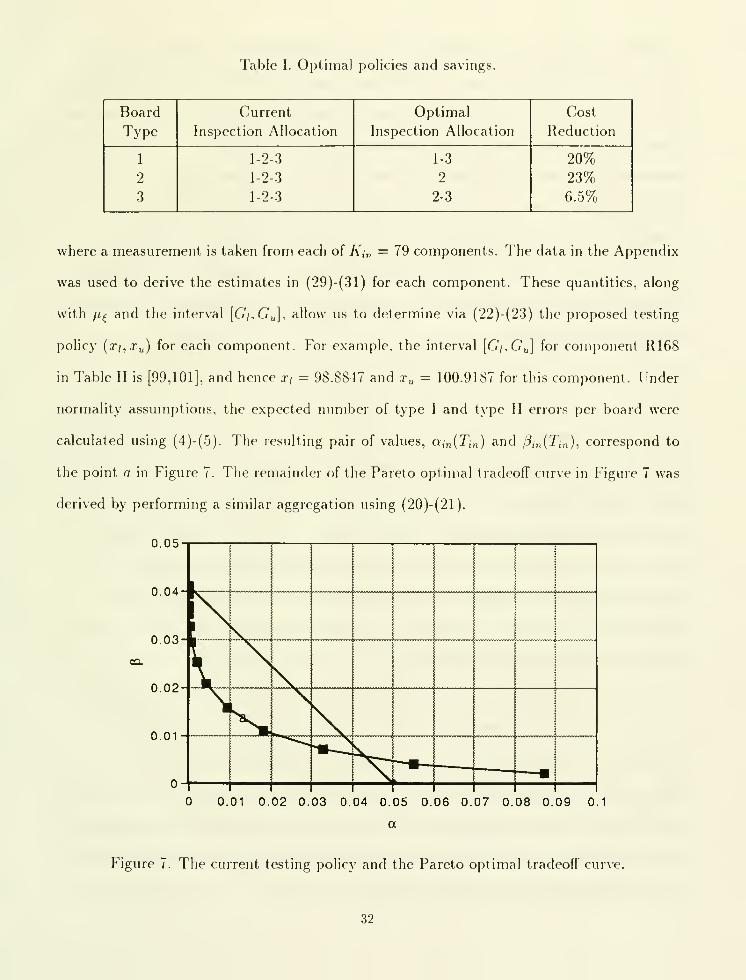
Table I. Optimal policies and savings.

Board

Type

Hewlett-Packard engineers have observed that about 55% of the rejected components at

the in circuit test are good components. Further analysis found that this percentage did

not vary significantly by board type. To illustrate how this performance compares to that

of our proposed testing policy, Figure 7 also shows a straight line that represents the set of

policies such that 55% of the rejected components are good components. If we had obtained

somewhat different estimates for a^ and a^, then the proposed policy would have been on

the tradeoff curve in the neighborhood of a, and a significant improvement over the current

pohcy would still be achieved. The percentage improvement in Figures 5 and 7 appear to be

of the same order of magnitude, which represents about a 5% reduction in inspection costs

if implemented systemwide.

5. Concluding Remarks

The model presented here is built on two key features: hierarchical test coverage and

measurement errors in the testing process. Although this model was developed in the frame-

work of circuit board assembly, these features are present in many other settings. Hierarchical

test coverage is a ver\- natural property when inspection is performed at different stages in a

manufacturing process; the increasing test coverage is then a direct consequence of the fact

that potential defects are added between inspection stages by the intermediate manufactur-

ing operations. Also, test measurements are typically subject to some noise, particularly in

the manufacturing of high precision products.

For the problem considered here, an optimal inspection policy could be pursued for a

modest size problem by discretizing the /—dimensional state space of defect types and the

curves that can be generated by the Pareto optimal policies in (20)-(21). Howe\er, the case

study reveals that the required precision in the parameter estimates are very difficult to

achieve, even after performing controlled experiments and aggregating similar component

types. As a result, we focus on developing a simple but systematic procedure for deriving

the cutoff limits that characterize the testing policy.

33

For three representative board types in the case study, the optimal inspection allocation

policy achieves a 10% to 20% reduction in expected inspection costs relative to the facility's

historical inspection policy, under the facility's historical testing policy. For the in circuit test

that detects defective components, the proposed testing policy significantly outperforms the

facility's historical testing policy on one board type, representing roughly a 5% reduction

in inspection costs. Since the cost of inspection represents about half of the total direct

manufacturing cost, these cost savings are significant. Moreover, both policies are relatively

ea^y to implement in practice.

The Hewlett-Packard facility is just beginning to apply our model. Since a thorough

investigation of measurement errors had never been undertaken at this facility, perhaps the

biggest contribution thus far has been the statistical analysis of the data. We encountered

many cases, previously unbeknownst to the facility's engineers, where the mean measurement

error was an order of magnitude larger than the variance of the measurement error: see the

tables in the Appendix for some examples. These tables are extremely useful for developing

some quick insights into the optimal testing policy. For example, resistors such as Rl-58,

R170 and R317 should perhaps not be tested (or at least ha^'e extremely slack cutoff limits),

since the measurement noise is so large relative to the true component noise. In contrast,

fairly tight cutoff limits can be set for most of the resistors, where o^ja^ is very small. The

facility has begun implementing the proposed testing policy, but has not yet implemented

the optimal inspection allocation policy. Although they plan to implement the latter polic}-,

the different inspection stages are managed by different people, and organizational barriers

still need to be overcome.

We started from a real problem at a specific industrial facility, and developed and ana-

lyzed a mathematical model to address this problem; however, the model is still relatively

crude. Nevertheless, it is hoped that this work will help future researchers find better mod-

els for the large number of problems of this nature that are beginning to emerge. With the

higher performance that is sought from manufactured products, it seems very likely that

34

inspection will become an increasingly important aspect of production management. With

respect to model refinement, we believe that a key shortcoming in this model is the assumed

independence between the distribution of measurement values at a given inspection stage

and the inspection policy used at previous stages. A natural first step towards modeling this

dependence is to assume that the true measurement value iij^f. depends on the inspection

policy at previous stages only through 6,n_], which is the expected number of type i defects

present on a board at stage n. Under this assumption, the dynamic programming framework

and the derivation of the Pareto optimal testing policies still hold; the only difference is that

the quantities a,„ and l3,„ in (7) and (16) are now functions of (5,,„_i, as well as the testing

policy T,„. All that remains is the formidable task of estimating the influence of S^n-i on

v\^^ from available data.

Acknowledgment

We are grateful to the people at the Hewlett-Packard plant in Andover. .MA for their

advice and their tremendous effort in helping us obtain the necessary data for our model.

We also thank Arnie Barnett and Steve Pollock for helpful discussions. This research is

supported by a grant from the Leaders for Manufacturing program at MIT and National

Science Foundation Grant Award No. DDM-9057297.

References

Albin, S. L. and D. J. Friedman. 1991. Off-Line Quality Control in Electronics Assembly:

Selecting the Critical Problem. Working Paper, Rutgers University, Piscataway, NJ.

Chevalier, P. B. 1992. Two Topics in Multistage Manufacturing Systems. Ph.D. dissertation,

Operations Research Center, MIT, Cambridge, MA.

35

Duncan, A. J. 1986. Quality Control and Industrial Statistics. Irwin, Homewood, II.

Eppen, G. D. and E. G. Hurst. 1974. Optimal Allocation of Inspection Stations in a Multi-

stage Production Process. Management Science 20, 1194-1200.

Garcia-Diaz, A., J. W. Foster, and M. Bonyuet. 1984. Dynamic Programming Analysis of

Special Multistage Inspection Systems. HE Transactions 16, 115-125.

Lindsay, G. F. and A. B. Bishop. 1967. Allocation of Screening Inspection EfFort-A DjTiamic-

Programming Approach. Management Science 10, 342-352.

Raz, T. 1986. A Survey of Models for Allocating Inspection Effort in Multistage Production

Systems. Journal of Quality Technology 18, 239-247.

Tang, C. S. 1991. Designing an Optimal Production System with Inspection. European

Journal of Operations Research 52, 45-54.

Villalobos, J. R., J. W. Foster, and R. L. Disney. 1992. Flexible Inspection System? for Serial

Multi-Stage Production Systems. Working Paper. Department of Industrial Engineering,

Texas A&M University, College Station, TX.

White, L. S. 1966. The Analysis of a Simple Class of Multistage Inspection Plans. Manage-

ment Science 9, 685-693.

Yum, B. J. and E. D. McDowell, E. D. 1981. The Optimal Allocation of Inspection EfTort in

a Class of Nonserial Production Systems. HE Transactions 13, 285-293.

36

Table II. Resistors.

Component

Table IV. Capacitors.

Component

Table VI. Diodes.

Component

Date Due

MIT IIBRARIES

3 IQflO 0071^71 R